Xception: Deep Learning with Depthwise Separable Convolutions

收录于 CVPR 2017 会议论文；IEEE DOI 10.1109/cvpr.2017.195；arXiv:1610.02357被引 21,081 次

Xception: Deep Learning with Depthwise Separable Convolutions

Xception：用深度可分离卷积做深度学习

François Chollet Affiliation: Google, Inc. Email: fchollet@google.com

Abstract

摘要

We present an interpretation of Inception modules in convolutional neural networks as being an intermediate step in-between regular convolution and the depthwise separable convolution operation (a depthwise convolution followed by a pointwise convolution). In this light, a depthwise separable convolution can be understood as an Inception module with a maximally large number of towers. This observation leads us to propose a novel deep convolutional neural network architecture inspired by Inception, where Inception modules have been replaced with depthwise separable convolutions. We show that this architecture, dubbed Xception, slightly outperforms Inception V3 on the ImageNet dataset (which Inception V3 was designed for), and significantly outperforms Inception V3 on a larger image classification dataset comprising 350 million images and 17,000 classes. Since the Xception architecture has the same number of parameters as Inception V3, the performance gains are not due to increased capacity but rather to a more efficient use of model parameters.

我们把卷积神经网络里的 Inception 模块，理解成普通卷积和 深度可分离卷积 （depthwise separable convolution，即一次深度卷积再接一次逐点卷积）之间的中间步骤。按这个看法，深度可分离卷积相当于塔的数量放到最大的 Inception 模块。由此我们提出一种受 Inception 启发的新的深度卷积网络：把 Inception 模块全部换成深度可分离卷积。这个结构叫做 Xception。它在 ImageNet（Inception V3 当初就是为这个数据集设计的）上略优于 Inception V3，在一个包含 3.5 亿张图像、17,000 类的更大规模图像分类数据集上则明显优于 Inception V3。Xception 与 Inception V3 的参数量相同，因此这些提升并不是因为容量变大，而是因为模型参数用得更有效。

1 Introduction

1 引言

Convolutional neural networks have emerged as the master algorithm in computer vision in recent years, and developing recipes for designing them has been a subject of considerable attention. The history of convolutional neural network design started with LeNet-style models [10], which were simple stacks of convolutions for feature extraction and max-pooling operations for spatial sub-sampling. In 2012, these ideas were refined into the AlexNet architecture [9], where convolution operations were being repeated multiple times in-between max-pooling operations, allowing the network to learn richer features at every spatial scale. What followed was a trend to make this style of network increasingly deeper, mostly driven by the yearly ILSVRC competition; first with Zeiler and Fergus in 2013 [25] and then with the VGG architecture in 2014 [18].

近年来，卷积神经网络已经成为计算机视觉里的主力学术方案，如何设计它们也因此受到很多关注。卷积网络设计的起点是 LeNet 风格的模型 [10]：用卷积提取特征，再用最大池化做空间下采样，一层层叠起来。2012 年，这些想法被改进成 AlexNet [9]：在两次最大池化之间会重复多次卷积，让网络在每个空间尺度上都能学到更丰富的特征。随后的趋势是把这种网络做得越来越深，主要动力来自每年的 ILSVRC 竞赛：先是 2013 年的 Zeiler 和 Fergus [25]，然后是 2014 年的 VGG [18]。

At this point a new style of network emerged, the Inception architecture, introduced by Szegedy et al. in 2014 [20] as GoogLeNet (Inception V1), later refined as Inception V2 [7], Inception V3 [21], and most recently Inception-ResNet [19]. Inception itself was inspired by the earlier Network-In-Network architecture [11]. Since its first introduction, Inception has been one of the best performing family of models on the ImageNet dataset [14], as well as internal datasets in use at Google, in particular JFT [5].

就在这个时候，出现了一种新的网络风格，也就是 Inception 结构。Szegedy 等人在 2014 年以 GoogLeNet（Inception V1）的形式提出 [20]，后来又发展成 Inception V2 [7]、Inception V3 [21]，以及最近的 Inception-ResNet [19]。Inception 本身受到更早的 Network-In-Network 结构 [11] 的启发。自问世以来，Inception 一直是 ImageNet [14] 上表现最好的模型家族之一，在 Google 内部使用的数据集上同样如此，尤其是 JFT [5]。

The fundamental building block of Inception-style models is the Inception module, of which several different versions exist. In figure 1 we show the canonical form of an Inception module, as found in the Inception V3 architecture. An Inception model can be understood as a stack of such modules. This is a departure from earlier VGG-style networks which were stacks of simple convolution layers.

Inception 风格模型的基本构件是 Inception 模块，它有若干不同版本。图 1 给出的是 Inception V3 里那种典型形式。一个 Inception 模型可以看成这些模块的堆叠。这和更早的、只是把简单卷积层叠起来的 VGG 风格网络已经不一样了。

While Inception modules are conceptually similar to convolutions (they are convolutional feature extractors), they empirically appear to be capable of learning richer representations with less parameters. How do they work, and how do they differ from regular convolutions? What design strategies come after Inception?

Inception 模块在概念上和卷积很接近（它们都是卷积式的特征提取器），但经验上看，它们往往能用更少的参数学到更丰富的表征。它们到底是怎么工作的，和普通卷积差在哪里？Inception 之后，设计策略又该往哪走？

1.1 The Inception hypothesis

1.1 Inception 假说

A convolution layer attempts to learn filters in a 3D space, with 2 spatial dimensions (width and height) and a channel dimension; thus a single convolution kernel is tasked with simultaneously mapping cross-channel correlations and spatial correlations.

一层卷积要在三维空间里学习滤波器，其中两个是空间维（宽和高），还有一个是通道维；于是单个卷积核必须同时映射通道之间的相关，以及空间上的相关。

This idea behind the Inception module is to make this process easier and more efficient by explicitly factoring it into a series of operations that would independently look at cross-channel correlations and at spatial correlations. More precisely, the typical Inception module first looks at cross-channel correlations via a set of 1x1 convolutions, mapping the input data into 3 or 4 separate spaces that are smaller than the original input space, and then maps all correlations in these smaller 3D spaces, via regular 3x3 or 5x5 convolutions. This is illustrated in figure 1. In effect, the fundamental hypothesis behind Inception is that cross-channel correlations and spatial correlations are sufficiently decoupled that it is preferable not to map them jointly [^1]. [^1]: A variant of the process is to independently look at width-wise correlations and height-wise correlations. This is implemented by some of the modules found in Inception V3, which alternate 7x1 and 1x7 convolutions. The use of such spatially separable convolutions has a long history in image processing and has been used in some convolutional neural network implementations since at least 2012 (possibly earlier).

1\times 1

Consider a simplified version of an Inception module that only uses one size of convolution (e.g. 3x3) and does not include an average pooling tower (figure 2). This Inception module can be reformulated as a large 1x1 convolution followed by spatial convolutions that would operate on non-overlapping segments of the output channels (figure 3). This observation naturally raises the question: what is the effect of the number of segments in the partition (and their size)? Would it be reasonable to make a much stronger hypothesis than the Inception hypothesis, and assume that cross-channel correlations and spatial correlations can be mapped completely separately?

3\times 3

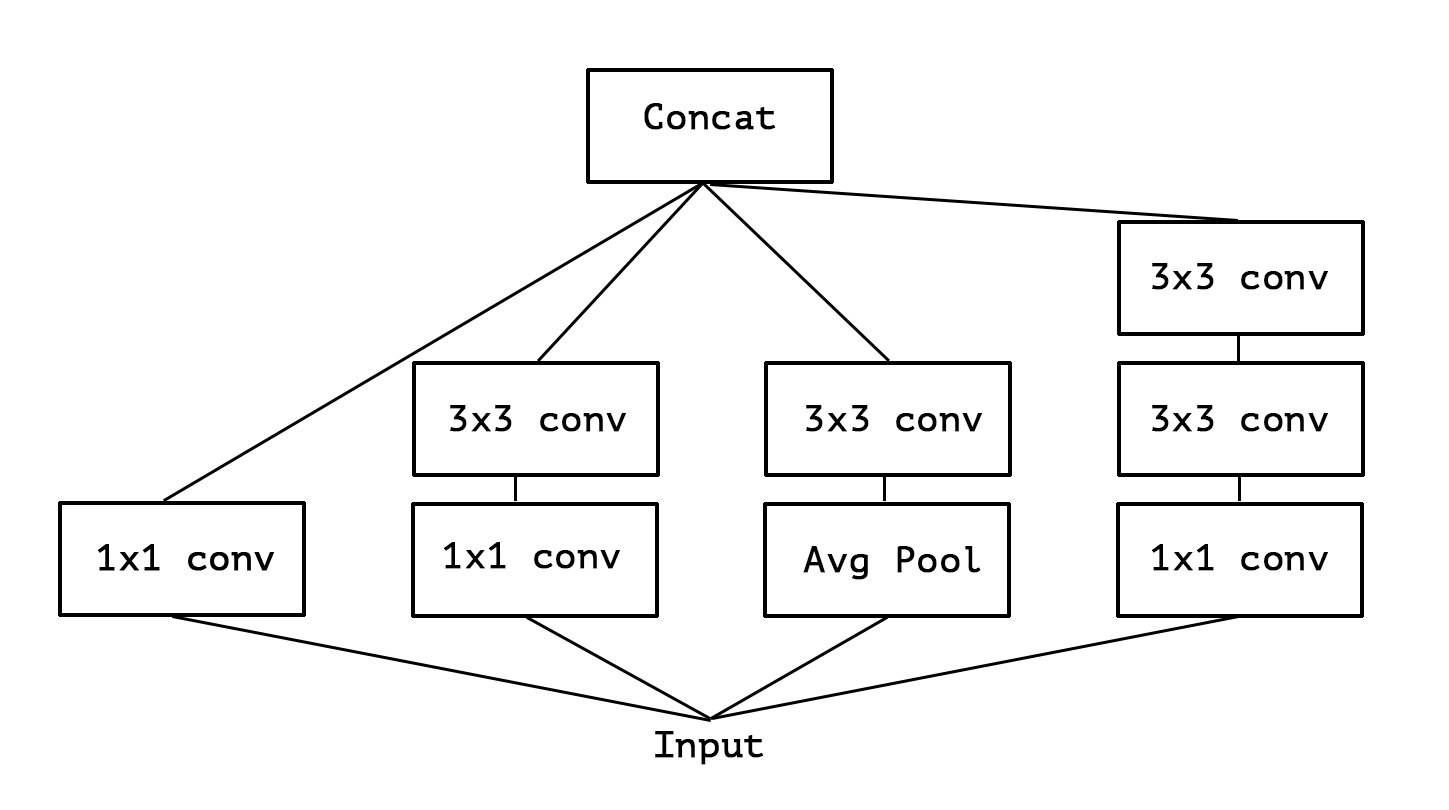
Figure 1: A canonical Inception module (Inception V3).

图 1：典型的 Inception 模块（Inception V3）。

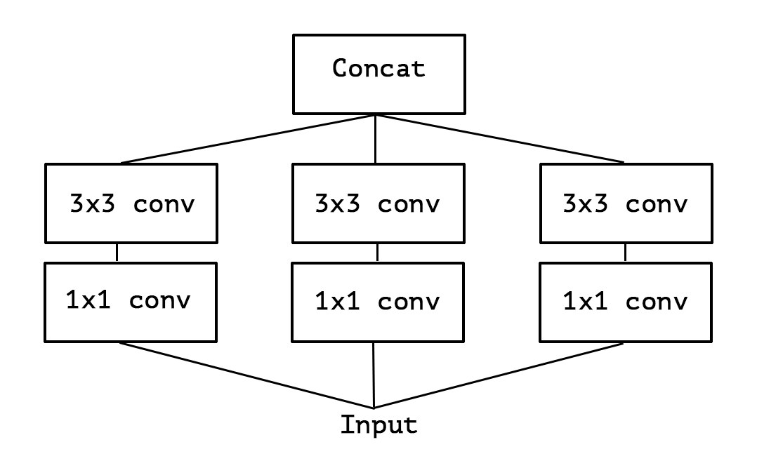
Figure 2: A simplified Inception module.

图 2：简化后的 Inception 模块。

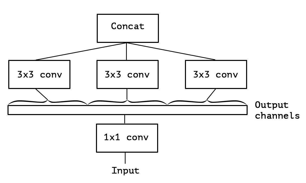
Figure 3: A strictly equivalent reformulation of the simplified Inception module.

图 3：与简化 Inception 模块严格等价的改写。

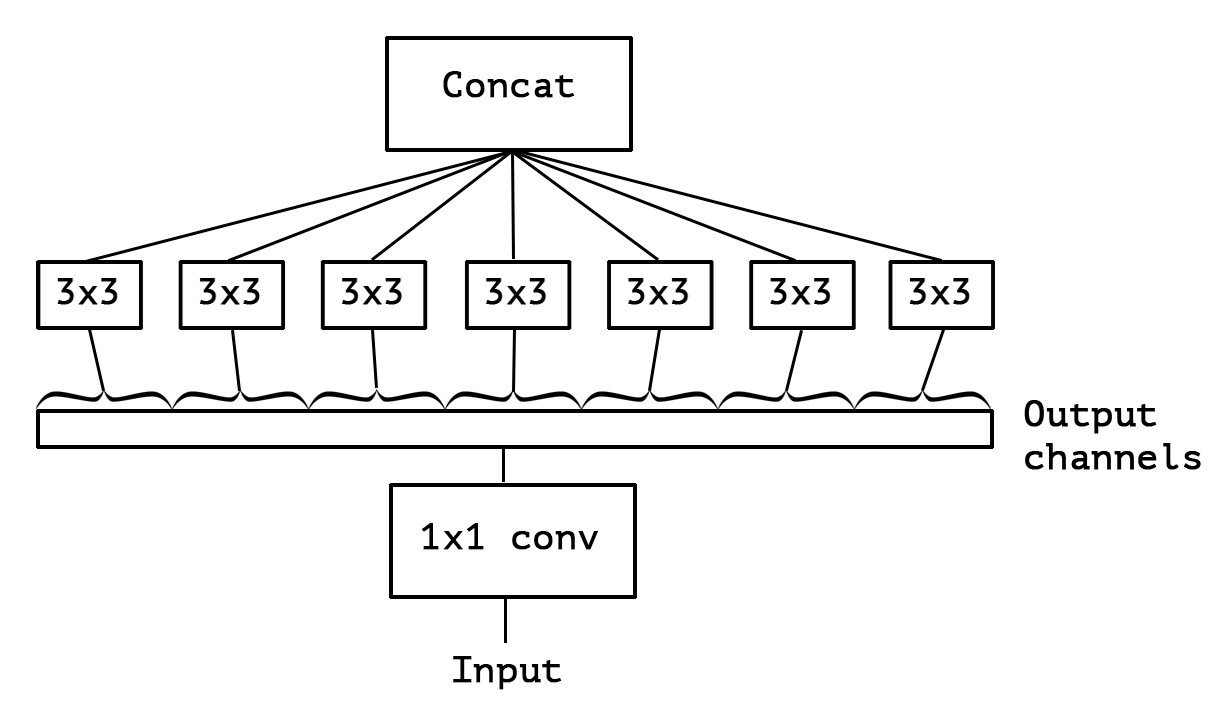
Figure 4: An “extreme” version of our Inception module, with one spatial convolution per output channel of the 1x1 convolution.

1\times 1

1.2 The continuum between convolutions and separable convolutions

1.2 卷积与可分离卷积之间的连续谱

An “extreme” version of an Inception module, based on this stronger hypothesis, would first use a 1x1 convolution to map cross-channel correlations, and would then separately map the spatial correlations of every output channel. This is shown in figure 4. We remark that this extreme form of an Inception module is almost identical to a depthwise separable convolution, an operation that has been used in neural network design as early as 2014 [15] and has become more popular since its inclusion in the TensorFlow framework [1] in 2016.

1\times 1

A depthwise separable convolution, commonly called “separable convolution” in deep learning frameworks such as TensorFlow and Keras, consists in a depthwise convolution, i.e. a spatial convolution performed independently over each channel of an input, followed by a pointwise convolution, i.e. a 1x1 convolution, projecting the channels output by the depthwise convolution onto a new channel space. This is not to be confused with a spatially separable convolution, which is also commonly called “separable convolution” in the image processing community.

1\times 1

Two minor differences between and “extreme” version of an Inception module and a depthwise separable convolution would be:

Inception 模块的“极端”版本和深度可分离卷积之间，还有两处小的差别：

• The order of the operations: depthwise separable convolutions as usually implemented (e.g. in TensorFlow) perform first channel-wise spatial convolution and then perform 1x1 convolution, whereas Inception performs the 1x1 convolution first.

1\times 1

• The presence or absence of a non-linearity after the first operation. In Inception, both operations are followed by a ReLU non-linearity, however depthwise separable convolutions are usually implemented without non-linearities.

第一步运算之后有没有非线性。在 Inception 里，两次运算后面都接 ReLU；而深度可分离卷积通常实现时不加非线性。

We argue that the first difference is unimportant, in particular because these operations are meant to be used in a stacked setting. The second difference might matter, and we investigate it in the experimental section (in particular see figure 10).

我们认为第一点差别并不重要，尤其是因为这些运算本来就是准备堆叠起来用的。第二点差别可能会有影响，我们会在实验部分考察它（尤其见图 10）。

We also note that other intermediate formulations of Inception modules that lie in between regular Inception modules and depthwise separable convolutions are also possible: in effect, there is a discrete spectrum between regular convolutions and depthwise separable convolutions, parametrized by the number of independent channel-space segments used for performing spatial convolutions. A regular convolution (preceded by a 1x1 convolution), at one extreme of this spectrum, corresponds to the single-segment case; a depthwise separable convolution corresponds to the other extreme where there is one segment per channel; Inception modules lie in between, dividing a few hundreds of channels into 3 or 4 segments. The properties of such intermediate modules appear not to have been explored yet.

1\times 1

Having made these observations, we suggest that it may be possible to improve upon the Inception family of architectures by replacing Inception modules with depthwise separable convolutions, i.e. by building models that would be stacks of depthwise separable convolutions. This is made practical by the efficient depthwise convolution implementation available in TensorFlow. In what follows, we present a convolutional neural network architecture based on this idea, with a similar number of parameters as Inception V3, and we evaluate its performance against Inception V3 on two large-scale image classification task.

基于这些观察，我们建议：或许可以把 Inception 模块换成深度可分离卷积，也就是搭出由深度可分离卷积堆起来的模型，从而改进 Inception 这一族结构。TensorFlow 里已经有高效的深度卷积实现，这件事因此变得可行。下面我们给出一个基于这个想法的卷积网络，参数量与 Inception V3 相近，并在两个大规模图像分类任务上与 Inception V3 对照。

2 Prior work

2 相关工作

The present work relies heavily on prior efforts in the following areas:

这项工作在很大程度上依赖以下几个方向已有的努力：

• Convolutional neural networks [10, 9, 25], in particular the VGG-16 architecture [18], which is schematically similar to our proposed architecture in a few respects.

卷积神经网络 [10, 9, 25]，尤其是 VGG-16 [18]，它在结构示意图上和我们提出的网络有若干相近之处。

• The Inception architecture family of convolutional neural networks [20, 7, 21, 19], which first demonstrated the advantages of factoring convolutions into multiple branches operating successively on channels and then on space.

Inception 这一族卷积网络 [20, 7, 21, 19]，它们最先展示了把卷积拆成多条分支、先处理通道再处理空间的好处。

• Depthwise separable convolutions, which our proposed architecture is entirely based upon. While the use of spatially separable convolutions in neural networks has a long history, going back to at least 2012 [12] (but likely even earlier), the depthwise version is more recent. Laurent Sifre developed depthwise separable convolutions during an internship at Google Brain in 2013, and used them in AlexNet to obtain small gains in accuracy and large gains in convergence speed, as well as a significant reduction in model size. An overview of his work was first made public in a presentation at ICLR 2014 [23]. Detailed experimental results are reported in Sifre’s thesis, section 6.2 [15]. This initial work on depthwise separable convolutions was inspired by prior research from Sifre and Mallat on transformation-invariant scattering [16, 15]. Later, a depthwise separable convolution was used as the first layer of Inception V1 and Inception V2 [20, 7]. Within Google, Andrew Howard [6] has introduced efficient mobile models called MobileNets using depthwise separable convolutions. Jin et al. in 2014 [8] and Wang et al. in 2016 [24] also did related work aiming at reducing the size and computational cost of convolutional neural networks using separable convolutions. Additionally, our work is only possible due to the inclusion of an efficient implementation of depthwise separable convolutions in the TensorFlow framework [1].

深度可分离卷积，我们提出的结构完全建立在它上面。空间可分离卷积在神经网络里的使用历史很长，至少可以追溯到 2012 年 [12]（很可能更早），深度方向的版本则更晚一些。Laurent Sifre 2013 年在 Google Brain 实习期间发展了深度可分离卷积，并把它们用进 AlexNet，精度上有小幅提升，收敛速度提高很多，模型体积也明显变小。这项工作的概述最早在 2014 年 ICLR 的一次报告里公开 [23]。详细实验结果写在 Sifre 的学位论文第 6.2 节 [15]。这批关于深度可分离卷积的早期工作，受到 Sifre 和 Mallat 关于变换不变散射（transformation-invariant scattering）研究的启发 [16, 15]。后来，Inception V1 和 Inception V2 的第一层也用了深度可分离卷积 [20, 7]。在 Google 内部，Andrew Howard [6] 用深度可分离卷积做出了面向移动端的高效模型 MobileNets。Jin 等人在 2014 年 [8] 以及 Wang 等人在 2016 年 [24] 也做了相关工作，目标是用可分离卷积减小卷积网络的体积和计算量。此外，TensorFlow 框架 [1] 里加入了深度可分离卷积的高效实现，我们的工作才成为可能。

• Residual connections, introduced by He et al. in [4], which our proposed architecture uses extensively.

残差连接，由 He 等人在 [4] 中提出，我们的结构大量使用了它。

3 The Xception architecture

3 Xception 结构

We propose a convolutional neural network architecture based entirely on depthwise separable convolution layers. In effect, we make the following hypothesis: that the mapping of cross-channels correlations and spatial correlations in the feature maps of convolutional neural networks can be entirely decoupled. Because this hypothesis is a stronger version of the hypothesis underlying the Inception architecture, we name our proposed architecture Xception, which stands for “Extreme Inception”.

我们提出一种完全由深度可分离卷积层构成的卷积网络。实际上，我们做了如下假设：卷积网络特征图里，通道之间的相关和空间上的相关，可以被 完全 解耦。这个假说是 Inception 结构背后那条假说的更强版本，因此我们把提出的结构叫做 Xception ，意思是 “Extreme Inception”。

A complete description of the specifications of the network is given in figure 5. The Xception architecture has 36 convolutional layers forming the feature extraction base of the network. In our experimental evaluation we will exclusively investigate image classification and therefore our convolutional base will be followed by a logistic regression layer. Optionally one may insert fully-connected layers before the logistic regression layer, which is explored in the experimental evaluation section (in particular, see figures 7 and 8). The 36 convolutional layers are structured into 14 modules, all of which have linear residual connections around them, except for the first and last modules.

网络的完整规格见图 5。Xception 用 36 个卷积层作为特征提取的主体。在我们的实验评估里只做图像分类，因此这个卷积主体后面会接一层逻辑回归。也可以选择在逻辑回归之前插入全连接层，这一点会在实验部分讨论（尤其见图 7 和图 8）。这 36 个卷积层被组织成 14 个模块，除了第一个和最后一个模块，其余模块周围都有线性残差连接。

In short, the Xception architecture is a linear stack of depthwise separable convolution layers with residual connections. This makes the architecture very easy to define and modify; it takes only 30 to 40 lines of code using a high-level library such as Keras [2] or TensorFlow-Slim [17], not unlike an architecture such as VGG-16 [18], but rather unlike architectures such as Inception V2 or V3 which are far more complex to define. An open-source implementation of Xception using Keras and TensorFlow is provided as part of the Keras Applications module^2, under the MIT license.

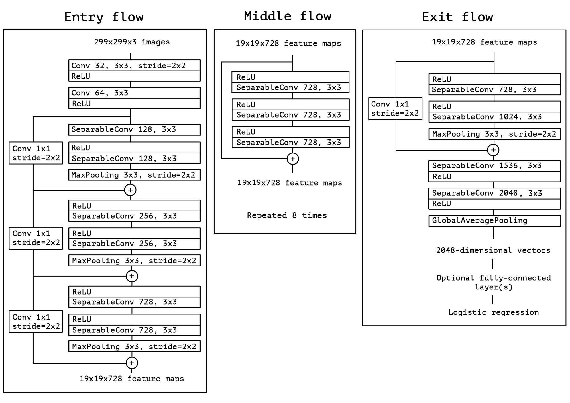
简而言之，Xception 是带残差连接的深度可分离卷积层的线性堆叠。这样的结构很容易定义和修改：用 Keras [2] 或 TensorFlow-Slim [17] 这类高层库，大约 30 到 40 行代码就能写完，这一点倒更像 VGG-16 [18]，而不像 Inception V2 或 V3 那种定义起来复杂得多的结构。我们在 Keras Applications 模块里提供了用 Keras 和 TensorFlow 实现的开源版本[^2]，采用 MIT 许可证。 [^2]： https://keras.io/applications/#xception

Figure 5: The Xception architecture: the data first goes through the entry flow, then through the middle flow which is repeated eight times, and finally through the exit flow. Note that all Convolution and SeparableConvolution layers are followed by batch normalization [7] (not included in the diagram). All SeparableConvolution layers use a depth multiplier of 1 (no depth expansion).

图 5：Xception 结构：数据先经过入口流（entry flow），再进入重复八次的中间流（middle flow），最后经过出口流（exit flow）。注意，所有 Convolution 和 SeparableConvolution 层后面都接批归一化 [7]（图中未画出）。所有 SeparableConvolution 层的深度乘数都设为 1（不做深度扩展）。

4 Experimental evaluation

4 实验评估

We choose to compare Xception to the Inception V3 architecture, due to their similarity of scale: Xception and Inception V3 have nearly the same number of parameters (table 3), and thus any performance gap could not be attributed to a difference in network capacity. We conduct our comparison on two image classification tasks: one is the well-known 1000-class single-label classification task on the ImageNet dataset [14], and the other is a 17,000-class multi-label classification task on the large-scale JFT dataset.

我们选择把 Xception 和 Inception V3 对照，是因为两者规模接近：参数量几乎相同（表 3），因此任何性能差距都不能归因于网络容量不同。对照在两个图像分类任务上进行：一个是人们熟悉的 ImageNet 数据集 [14] 上的 1000 类单标签分类，另一个是大规模 JFT 数据集上的 17,000 类多标签分类。

4.1 The JFT dataset

4.1 JFT 数据集

JFT is an internal Google dataset for large-scale image classification dataset, first introduced by Hinton et al. in [5], which comprises over 350 million high-resolution images annotated with labels from a set of 17,000 classes. To evaluate the performance of a model trained on JFT, we use an auxiliary dataset, FastEval14k .

JFT 是 Google 内部用于大规模图像分类的数据集，最早由 Hinton 等人在 [5] 中介绍，包含超过 3.5 亿张高分辨率图像，标注来自 17,000 个类别。为了评估在 JFT 上训练的模型，我们使用一个辅助数据集 FastEval14k 。

FastEval14k is a dataset of 14,000 images with dense annotations from about 6,000 classes (36.5 labels per image on average). On this dataset we evaluate performance using Mean Average Precision for top 100 predictions (MAP@100), and we weight the contribution of each class to MAP@100 with a score estimating how common (and therefore important) the class is among social media images. This evaluation procedure is meant to capture performance on frequently occurring labels from social media, which is crucial for production models at Google.

FastEval14k 包含 14,000 张图像，带有来自约 6,000 个类别的稠密标注（平均每张图 36.5 个标签）。在这个数据集上，我们用前 100 个预测的平均精度均值（MAP@100）来评估，并且按每个类别在社交媒体图像中有多常见（因此有多重要）的估计分数，为它对 MAP@100 的贡献加权。这套评估程序是为了抓住社交媒体里经常出现的标签上的表现，这对 Google 的生产模型很关键。

4.2 Optimization configuration

4.2 优化配置

A different optimization configuration was used for ImageNet and JFT:

ImageNet 和 JFT 使用了不同的优化配置：

• On ImageNet: - Optimizer: SGD - Momentum: 0.9 - Initial learning rate: 0.045 - Learning rate decay: decay of rate 0.94 every 2 epochs

在 ImageNet 上：优化器为 SGD；动量为 0.9；初始学习率为 0.045；学习率衰减为每 2 个 epoch 按 0.94 的比率衰减。

• On JFT: - Optimizer: RMSprop [22] - Momentum: 0.9 - Initial learning rate: 0.001 - Learning rate decay: decay of rate 0.9 every 3,000,000 samples

在 JFT 上：优化器为 RMSprop [22]；动量为 0.9；初始学习率为 0.001；学习率衰减为每 3,000,000 个样本按 0.9 的比率衰减。

For both datasets, the same exact same optimization configuration was used for both Xception and Inception V3. Note that this configuration was tuned for best performance with Inception V3; we did not attempt to tune optimization hyperparameters for Xception. Since the networks have different training profiles (figure 6), this may be suboptimal, especially on the ImageNet dataset, on which the optimization configuration used had been carefully tuned for Inception V3.

在两个数据集上，Xception 和 Inception V3 使用了完全相同的优化配置。需要说明的是，这套配置是为了让 Inception V3 表现最好而调过的；我们没有尝试为 Xception 再调优化超参数。由于两条网络的训练曲线并不一样（图 6），这样可能并非最优，在 ImageNet 上尤其如此，因为那里用的优化配置当初是专门为 Inception V3 仔细调过的。

Additionally, all models were evaluated using Polyak averaging [13] at inference time.

此外，所有模型在推断时都使用了 Polyak 平均 [13]。

4.3 Regularization configuration

4.3 正则配置

4e-5

4e-5

• Dropout: For the ImageNet experiments, both models include a dropout layer of rate 0.5 before the logistic regression layer. For the JFT experiments, no dropout was included due to the large size of the dataset which made overfitting unlikely in any reasonable amount of time.

Dropout ： 在 ImageNet 实验里，两个模型都在逻辑回归层之前加入了比率为 0.5 的 dropout 层。在 JFT 实验里没有加 dropout，因为数据集很大，在任何合理的训练时间内都不太可能过拟合。

• Auxiliary loss tower: The Inception V3 architecture may optionally include an auxiliary tower which backpropagates the classification loss earlier in the network, serving as an additional regularization mechanism. For simplicity, we choose not to include this auxiliary tower in any of our models.

辅助损失塔 ： Inception V3 结构可以选用一座辅助塔，把分类损失更早地反传到网络前部，作为额外的正则手段。为简单起见，我们决定在所有模型里都不加这座辅助塔。

4.4 Training infrastructure

4.4 训练基础设施

All networks were implemented using the TensorFlow framework [1] and trained on 60 NVIDIA K80 GPUs each. For the ImageNet experiments, we used data parallelism with synchronous gradient descent to achieve the best classification performance, while for JFT we used asynchronous gradient descent so as to speed up training. The ImageNet experiments took approximately 3 days each, while the JFT experiments took over one month each. The JFT models were not trained to full convergence, which would have taken over three month per experiment.

所有网络都用 TensorFlow 框架 [1] 实现，并各自在 60 块 NVIDIA K80 GPU 上训练。ImageNet 实验采用数据并行和 同步 梯度下降，以获得最好的分类表现；JFT 实验则用 异步 梯度下降，以便加快训练。每组 ImageNet 实验大约需要 3 天，每组 JFT 实验则超过一个月。JFT 上的模型并没有训到完全收敛，那样的话每组实验会超过三个月。

4.5 Comparison with Inception V3

4.5 与 Inception V3 的对照

4.5.1 Classification performance All evaluations were run with a single crop of the inputs images and a single model. ImageNet results are reported on the validation set rather than the test set (i.e. on the non-blacklisted images from the validation set of ILSVRC 2012). JFT results are reported after 30 million iterations (one month of training) rather than after full convergence. Results are provided in table 1 and table 2, as well as figure 6, figure 7, figure 8. On JFT, we tested both versions of our networks that did not include any fully-connected layers, and versions that included two fully-connected layers of 4096 units each before the logistic regression layer.

4.5.1 分类表现 所有评估都只用输入图像的单裁，并且只用单个模型。ImageNet 的结果报告在验证集而不是测试集上（也就是 ILSVRC 2012 验证集里未被列入黑名单的图像）。JFT 的结果报告的是 3000 万次迭代之后（训练一个月），而不是完全收敛之后。结果见表 1、表 2，以及图 6、图 7、图 8。在 JFT 上，我们既测试了不含任何全连接层的版本，也测试了在逻辑回归层之前加入两层各 4096 个单元的全连接层的版本。

On ImageNet, Xception shows marginally better results than Inception V3. On JFT, Xception shows a 4.3% relative improvement on the FastEval14k MAP@100 metric. We also note that Xception outperforms ImageNet results reported by He et al. for ResNet-50, ResNet-101 and ResNet-152 [4].

在 ImageNet 上，Xception 比 Inception V3 略好。在 JFT 上，Xception 在 FastEval14k 的 MAP@100 指标上有约 4.3% 的相对提升。我们还注意到，Xception 超过了 He 等人报告的 ResNet-50、ResNet-101 和 ResNet-152 在 ImageNet 上的结果 [4]。

Top-1 accuracy Top-5 accuracy VGG-16 0.715 0.901 ResNet-152 0.770 0.933 Inception V3 0.782 0.941 Xception 0.790 0.945 Table 1: Classification performance comparison on ImageNet (single crop, single model). VGG-16 and ResNet-152 numbers are only included as a reminder. The version of Inception V3 being benchmarked does not include the auxiliary tower.

	Top-1 accuracy	Top-5 accuracy
VGG-16	0.715	0.901
ResNet-152	0.770	0.933
Inception V3	0.782	0.941
Xception	0.790	0.945

Top-1 精度 Top-5 精度 VGG-16 0.715 0.901 ResNet-152 0.770 0.933 Inception V3 0.782 0.941 Xception 0.790 0.945 表 1：ImageNet 上的分类表现对照（单裁、单模型）。VGG-16 和 ResNet-152 的数字只是作为参照列出。这里评估的 Inception V3 版本不含辅助塔。

	Top-1 精度	Top-5 精度
VGG-16	0.715	0.901
ResNet-152	0.770	0.933
Inception V3	0.782	0.941
Xception	0.790	0.945

FastEval14k MAP@100 Inception V3 - no FC layers 6.36 Xception - no FC layers 6.70 Inception V3 with FC layers 6.50 Xception with FC layers 6.78 Table 2: Classification performance comparison on JFT (single crop, single model).

	FastEval14k MAP@100
Inception V3 - no FC layers	6.36
Xception - no FC layers	6.70
Inception V3 with FC layers	6.50
Xception with FC layers	6.78

FastEval14k MAP@100 Inception V3 - 无全连接层 6.36 Xception - 无全连接层 6.70 Inception V3 含全连接层 6.50 Xception 含全连接层 6.78 表 2：JFT 上的分类表现对照（单裁、单模型）。

	FastEval14k MAP@100
Inception V3 - 无全连接层	6.36
Xception - 无全连接层	6.70
Inception V3 含全连接层	6.50
Xception 含全连接层	6.78

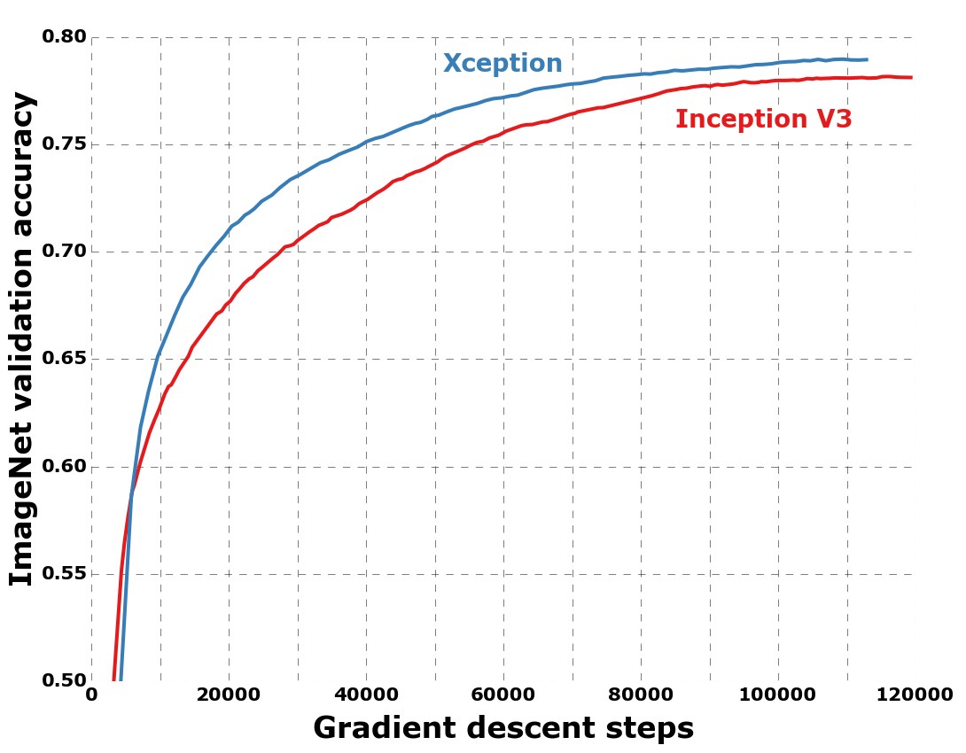
Figure 6: Training profile on ImageNet

图 6：ImageNet 上的训练曲线

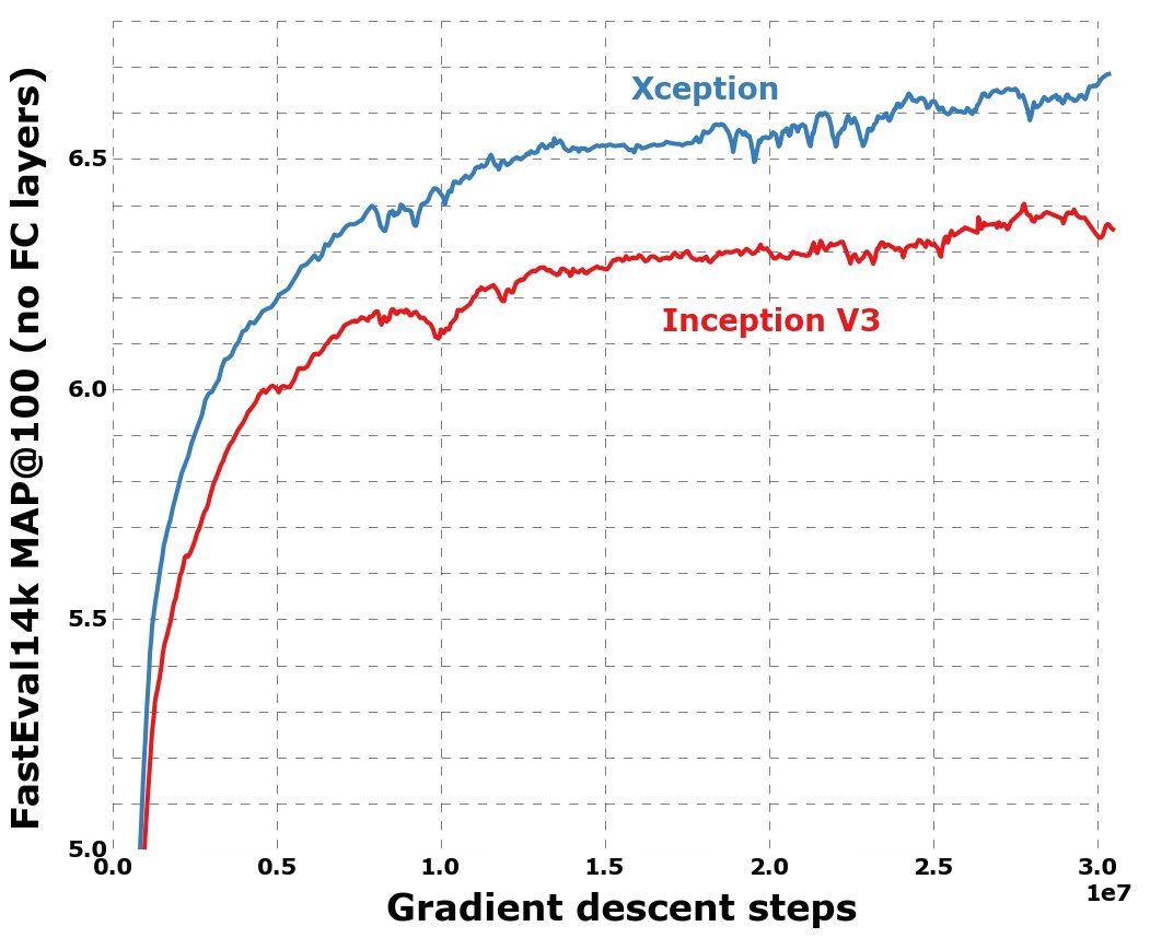
Figure 7: Training profile on JFT, without fully-connected layers

图 7：JFT 上不含全连接层的训练曲线

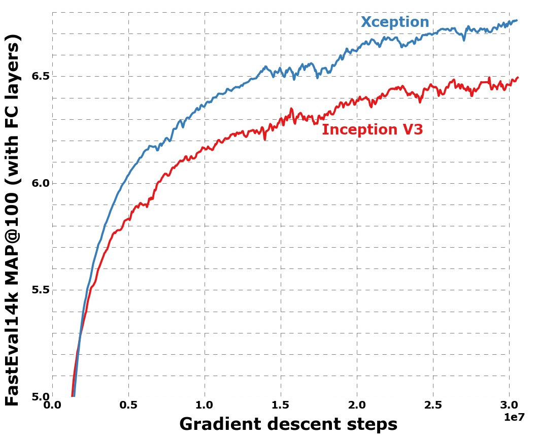
Figure 8: Training profile on JFT, with fully-connected layers

图 8：JFT 上含全连接层的训练曲线

The Xception architecture shows a much larger performance improvement on the JFT dataset compared to the ImageNet dataset. We believe this may be due to the fact that Inception V3 was developed with a focus on ImageNet and may thus be by design over-fit to this specific task. On the other hand, neither architecture was tuned for JFT. It is likely that a search for better hyperparameters for Xception on ImageNet (in particular optimization parameters and regularization parameters) would yield significant additional improvement.

和 ImageNet 相比，Xception 在 JFT 数据集上的提升要大得多。我们认为，这可能是因为 Inception V3 当初主要对着 ImageNet 来设计，因而在结构上可能过拟合到了这个特定任务。另一方面，两种结构都没有为 JFT 单独调过。如果在 ImageNet 上为 Xception 再搜索更好的超参数（尤其是优化参数和正则参数），很可能还会带来可观的额外提升。

4.5.2 Size and speed Parameter count Steps/second Inception V3 23,626,728 31 Xception 22,855,952 28 Table 3: Size and training speed comparison.

	Parameter count	Steps/second
Inception V3	23,626,728	31
Xception	22,855,952	28

4.5.2 规模和速度 参数量 步数/秒 Inception V3 23,626,728 31 Xception 22,855,952 28 表 3：规模和训练速度对照。

	参数量	步数/秒
Inception V3	23,626,728	31
Xception	22,855,952	28

In table 3 we compare the size and speed of Inception V3 and Xception. Parameter count is reported on ImageNet (1000 classes, no fully-connected layers) and the number of training steps (gradient updates) per second is reported on ImageNet with 60 K80 GPUs running synchronous gradient descent. Both architectures have approximately the same size (within 3.5%), and Xception is marginally slower. We expect that engineering optimizations at the level of the depthwise convolution operations can make Xception faster than Inception V3 in the near future. The fact that both architectures have almost the same number of parameters indicates that the improvement seen on ImageNet and JFT does not come from added capacity but rather from a more efficient use of the model parameters.

表 3 对照了 Inception V3 和 Xception 的规模与速度。参数量按 ImageNet（1000 类、不含全连接层）统计；每秒训练步数（梯度更新次数）按 ImageNet、60 块 K80 GPU、同步梯度下降来统计。两种结构的规模大致相同（差距在 3.5% 以内），Xception 略慢一些。我们预期，如果在深度卷积运算这一层再做工程优化，不久之后 Xception 可以比 Inception V3 更快。两边参数量几乎一样，说明在 ImageNet 和 JFT 上看到的提升并不是来自容量增加，而是来自更有效地使用了模型参数。

4.6 Effect of the residual connections

4.6 残差连接的作用

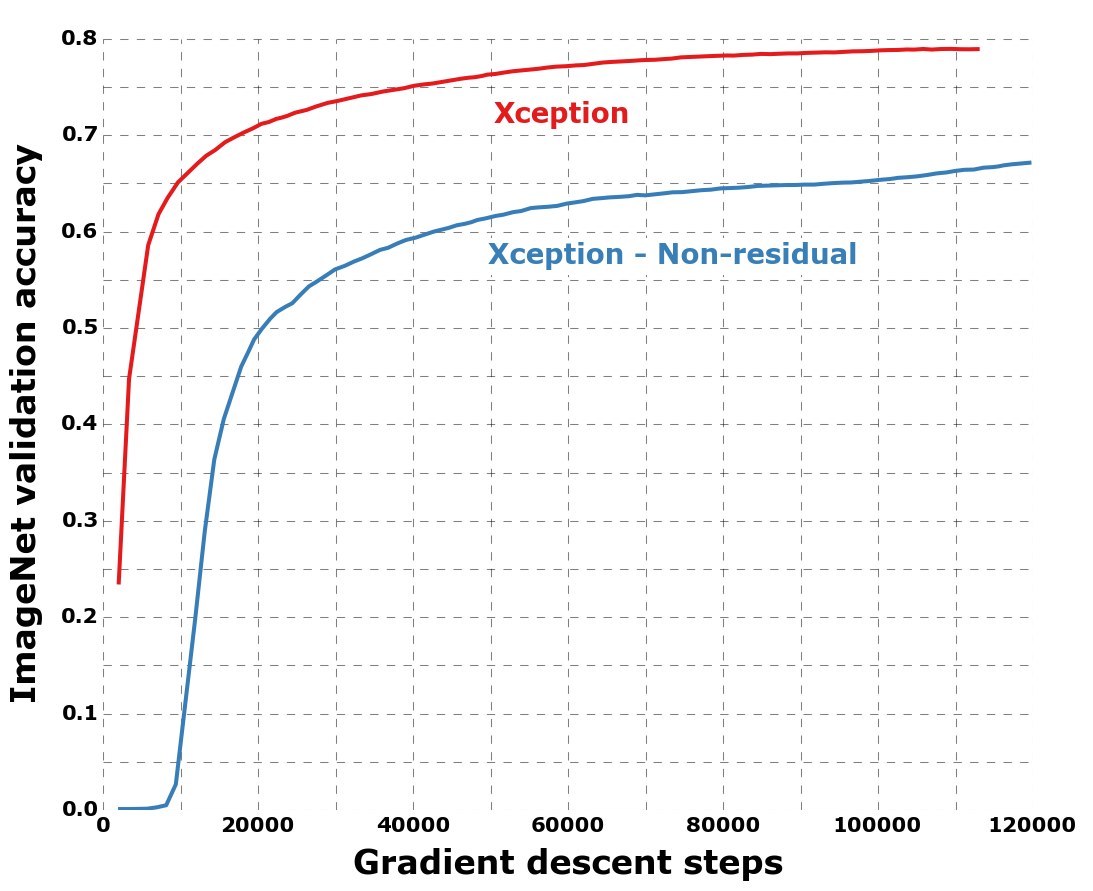
Figure 9: Training profile with and without residual connections.

图 9：有无残差连接的训练曲线。

To quantify the benefits of residual connections in the Xception architecture, we benchmarked on ImageNet a modified version of Xception that does not include any residual connections. Results are shown in figure 9. Residual connections are clearly essential in helping with convergence, both in terms of speed and final classification performance. However we will note that benchmarking the non-residual model with the same optimization configuration as the residual model may be uncharitable and that better optimization configurations might yield more competitive results.

为了量化残差连接在 Xception 结构里的好处，我们在 ImageNet 上评估了一个去掉所有残差连接的修改版 Xception。结果见图 9。残差连接对收敛显然是关键的，无论是速度还是最终分类表现都是如此。不过我们要说明，用和残差模型完全相同的优化配置去评估无残差模型，可能对后者并不公平；如果换一套更好的优化配置，无残差模型也许会更有竞争力。

Additionally, let us note that this result merely shows the importance of residual connections for this specific architecture, and that residual connections are in no way required in order to build models that are stacks of depthwise separable convolutions. We also obtained excellent results with non-residual VGG-style models where all convolution layers were replaced with depthwise separable convolutions (with a depth multiplier of 1), superior to Inception V3 on JFT at equal parameter count.

另外需要说明，这个结果只表明残差连接 对这一特定结构 很重要，并不意味着要搭建由深度可分离卷积堆起来的模型，残差连接就 必不可少 。我们还做过不含残差的 VGG 风格模型，只是把所有卷积层换成深度可分离卷积（深度乘数为 1），在参数量相同的情况下，它们在 JFT 上的结果优于 Inception V3。

4.7 Effect of an intermediate activation after pointwise convolutions

4.7 逐点卷积之后加入中间激活的影响

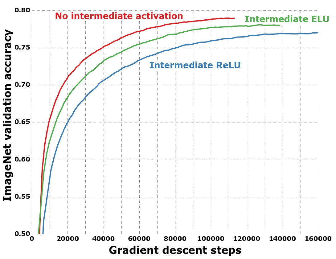
Figure 10: Training profile with different activations between the depthwise and pointwise operations of the separable convolution layers.

图 10：可分离卷积层中，深度卷积与逐点卷积之间使用不同激活时的训练曲线。

We mentioned earlier that the analogy between depthwise separable convolutions and Inception modules suggests that depthwise separable convolutions should potentially include a non-linearity between the depthwise and pointwise operations. In the experiments reported so far, no such non-linearity was included. However we also experimentally tested the inclusion of either ReLU or ELU [3] as intermediate non-linearity. Results are reported on ImageNet in figure 10, and show that the absence of any non-linearity leads to both faster convergence and better final performance.

前面说过，深度可分离卷积和 Inception 模块的类比意味着：在深度卷积和逐点卷积之间，也许应该加一个非线性。到目前为止报告的实验里，并没有加这种非线性。不过我们也实验过用 ReLU 或 ELU [3] 作为中间非线性。ImageNet 上的结果见图 10：不加任何非线性时，收敛更快，最终表现也更好。

This is a remarkable observation, since Szegedy et al. report the opposite result in [21] for Inception modules. It may be that the depth of the intermediate feature spaces on which spatial convolutions are applied is critical to the usefulness of the non-linearity: for deep feature spaces (e.g. those found in Inception modules) the non-linearity is helpful, but for shallow ones (e.g. the 1-channel deep feature spaces of depthwise separable convolutions) it becomes harmful, possibly due to a loss of information.

这个观察相当值得注意，因为 Szegedy 等人在 [21] 里对 Inception 模块报告的是相反的结果。中间特征空间的深度，也就是空间卷积作用在其上的那个空间有多深，可能对非线性是否有用至关重要：对很深的特征空间（例如 Inception 模块里的那些），非线性是有帮助的；对很浅的特征空间（例如深度可分离卷积里只有 1 个通道那么深的特征空间），非线性反而有害，可能是因为损失了信息。

5 Future directions

5 未来方向

We noted earlier the existence of a discrete spectrum between regular convolutions and depthwise separable convolutions, parametrized by the number of independent channel-space segments used for performing spatial convolutions. Inception modules are one point on this spectrum. We showed in our empirical evaluation that the extreme formulation of an Inception module, the depthwise separable convolution, may have advantages over regular a regular Inception module. However, there is no reason to believe that depthwise separable convolutions are optimal. It may be that intermediate points on the spectrum, lying between regular Inception modules and depthwise separable convolutions, hold further advantages. This question is left for future investigation.

前面我们指出，普通卷积和深度可分离卷积之间存在一条离散的谱，参数是用来做空间卷积的、相互独立的通道空间分段数目。Inception 模块是这条谱上的一个点。经验评估表明，Inception 模块的极端形式，也就是深度可分离卷积，可能比普通的 Inception 模块更有优势。不过，没有理由认为深度可分离卷积就是最优的。谱上介于普通 Inception 模块和深度可分离卷积之间的那些中间点，或许还藏着更多好处。这个问题留给以后研究。

6 Conclusions

6 结论

We showed how convolutions and depthwise separable convolutions lie at both extremes of a discrete spectrum, with Inception modules being an intermediate point in between. This observation has led to us to propose replacing Inception modules with depthwise separable convolutions in neural computer vision architectures. We presented a novel architecture based on this idea, named Xception, which has a similar parameter count as Inception V3. Compared to Inception V3, Xception shows small gains in classification performance on the ImageNet dataset and large gains on the JFT dataset. We expect depthwise separable convolutions to become a cornerstone of convolutional neural network architecture design in the future, since they offer similar properties as Inception modules, yet are as easy to use as regular convolution layers.

我们说明了，卷积和深度可分离卷积分别落在一条离散谱的两端，Inception 模块则是中间的一个点。基于这一观察，我们建议在神经计算机视觉结构里，用深度可分离卷积替换 Inception 模块。我们给出了按这个想法设计的新结构，命名为 Xception，其参数量与 Inception V3 相近。与 Inception V3 相比，Xception 在 ImageNet 上的分类表现有小幅提升，在 JFT 上的提升则更大。我们预期，深度可分离卷积将来会成为卷积网络结构设计里的一块基石：它们有和 Inception 模块相近的性质，用起来却像普通卷积层一样简单。

References

参考文献

[1] M. Abadi, A. Agarwal, P. Barham, E. Brevdo, Z. Chen, C. Citro, G. S. Corrado, A. Davis, J. Dean, M. Devin, S. Ghemawat, I. Goodfellow, A. Harp, G. Irving, M. Isard, Y. Jia, R. Jozefowicz, L. Kaiser, M. Kudlur, J. Levenberg, D. Mané, R. Monga, S. Moore, D. Murray, C. Olah, M. Schuster, J. Shlens, B. Steiner, I. Sutskever, K. Talwar, P. Tucker, V. Vanhoucke, V. Vasudevan, F. Viégas, O. Vinyals, P. Warden, M. Wattenberg, M. Wicke, Y. Yu, and X. Zheng. TensorFlow: Large-scale machine learning on heterogeneous systems, 2015. Software available from tensorflow.org. [2] F. Chollet. Keras. https://github.com/fchollet/keras, 2015. [3] D.-A. Clevert, T. Unterthiner, and S. Hochreiter. Fast and accurate deep network learning by exponential linear units (elus). arXiv preprint arXiv:1511.07289 , 2015. [4] K. He, X. Zhang, S. Ren, and J. Sun. Deep residual learning for image recognition. arXiv preprint arXiv:1512.03385 , 2015. [5] G. Hinton, O. Vinyals, and J. Dean. Distilling the knowledge in a neural network, 2015. [6] A. Howard. Mobilenets: Efficient convolutional neural networks for mobile vision applications. Forthcoming. [7] S. Ioffe and C. Szegedy. Batch normalization: Accelerating deep network training by reducing internal covariate shift. In Proceedings of The 32nd International Conference on Machine Learning , pages 448-456, 2015. [8] J. Jin, A. Dundar, and E. Culurciello. Flattened convolutional neural networks for feedforward acceleration. arXiv preprint arXiv:1412.5474 , 2014. [9] A. Krizhevsky, I. Sutskever, and G. E. Hinton. Imagenet classification with deep convolutional neural networks. In Advances in neural information processing systems , pages 1097-1105, 2012. [10] Y. LeCun, L. Jackel, L. Bottou, C. Cortes, J. S. Denker, H. Drucker, I. Guyon, U. Muller, E. Sackinger, P. Simard, et al. Learning algorithms for classification: A comparison on handwritten digit recognition. Neural networks: the statistical mechanics perspective , 261:276, 1995.

[11] M. Lin, Q. Chen, and S. Yan. Network in network. arXiv preprint arXiv:1312.4400 , 2013. [12] F. Mamalet and C. Garcia. Simplifying ConvNets for Fast Learning. In International Conference on Artificial Neural Networks (ICANN 2012) , pages 58-65. Springer, 2012. [13] B. T. Polyak and A. B. Juditsky. Acceleration of stochastic approximation by averaging. SIAM J. Control Optim. , 30(4):838-855, July 1992. [14] O. Russakovsky, J. Deng, H. Su, J. Krause, S. Satheesh, S. Ma, Z. Huang, A. Karpathy, A. Khosla, M. Bernstein, et al. Imagenet large scale visual recognition challenge. 2014. [15] L. Sifre. Rigid-motion scattering for image classification, 2014. Ph.D. thesis. [16] L. Sifre and S. Mallat. Rotation, scaling and deformation invariant scattering for texture discrimination. In 2013 IEEE Conference on Computer Vision and Pattern Recognition, Portland, OR, USA, June 23-28, 2013 , pages 1233-1240, 2013. [17] N. Silberman and S. Guadarrama. Tf-slim, 2016. [18] K. Simonyan and A. Zisserman. Very deep convolutional networks for large-scale image recognition. arXiv preprint arXiv:1409.1556 , 2014. [19] C. Szegedy, S. Ioffe, and V. Vanhoucke. Inception-v4, inception-resnet and the impact of residual connections on learning. arXiv preprint arXiv:1602.07261 , 2016. [20] C. Szegedy, W. Liu, Y. Jia, P. Sermanet, S. Reed, D. Anguelov, D. Erhan, V. Vanhoucke, and A. Rabinovich. Going deeper with convolutions. In Proceedings of the IEEE Conference on Computer Vision and Pattern Recognition , pages 1-9, 2015.

[21] C. Szegedy, V. Vanhoucke, S. Ioffe, J. Shlens, and Z. Wojna. Rethinking the inception architecture for computer vision. arXiv preprint arXiv:1512.00567 , 2015. [22] T. Tieleman and G. Hinton. Divide the gradient by a running average of its recent magnitude. COURSERA: Neural Networks for Machine Learning, 4, 2012. Accessed: 2015-11-05. [23] V. Vanhoucke. Learning visual representations at scale. ICLR, 2014. [24] M. Wang, B. Liu, and H. Foroosh. Factorized convolutional neural networks. arXiv preprint arXiv:1608.04337 , 2016. [25] M. D. Zeiler and R. Fergus. Visualizing and understanding convolutional networks. In Computer Vision-ECCV 2014 , pages 818-833. Springer, 2014.