Efficient Neural Audio Synthesis

高效的神经音频合成

Nal Kalchbrenner * 1
Erich Elsen * 2
Karen Simonyan 1
Florian Stimberg 1
Aäron van den Oord 1
Seb Noury 1
Norman Casagrande 1
Edward Lockhart 1
Sander Dieleman 1
Koray Kavukcuoglu 1
*Equal contribution 1DeepMind 2Google Brain. Correspondence to: Nal Kalchbrenner nalk@google.com.
Proceedings of the 35th International Conference on Machine Learning, Stockholm, Sweden, PMLR 80, 2018. Copyright 2018 by the author(s).

Abstract

摘要

Sequential models achieve state-of-the-art results in audio, visual and textual domains with respect to both estimating the data distribution and generating high-quality samples. Efficient sampling for this class of models has however remained an elusive problem. With a focus on text-to-speech synthesis, we describe a set of general techniques for reducing sampling time while maintaining high output quality. We first describe a single-layer recurrent neural network, the WaveRNN, with a dual softmax layer that matches the quality of the state-of-the-art WaveNet model. The compact form of the network makes it possible to generate 24 kHz 16-bit audio 4× faster than real time on a GPU. Second, we apply a weight pruning technique to reduce the number of weights in the WaveRNN. We find that, for a constant number of parameters, large sparse networks perform better than small dense networks and this relationship holds for sparsity levels beyond 96%. The small number of weights in a Sparse WaveRNN makes it possible to sample high-fidelity audio on a mobile CPU in real time. Finally, we propose a new generation scheme based on subscaling that folds a long sequence into a batch of shorter sequences and allows one to generate multiple samples at once. The Subscale WaveRNN produces 16 samples per step without loss of quality and offers an orthogonal method for increasing sampling efficiency.

序列模型在音频、视觉和文本领域，无论是估计数据分布还是生成高质量样本，都达到了当时最好的结果。但对这类模型做高效采样，仍然不好解决。我们把重点放在文本转语音上，介绍一组在保持输出质量的同时缩短采样时间的通用做法。首先给出单层循环网络 WaveRNN，它带有双 softmax 层，音质可以赶上当时最好的 WaveNet。网络形式紧凑，使得在 GPU 上能以 4 倍于实时的速度生成 24 kHz、16 位音频。其次，我们用权重剪枝减少 WaveRNN 中的权数量。我们发现：在参数量固定时，大而稀疏的网络优于小而稠密的网络，而且这一关系在稀疏度超过 96% 时仍然成立。Sparse WaveRNN 的权数量很少，因而可以在手机 CPU 上实时采样出高保真音频。最后，我们提出一种基于子尺度的生成方案：把长序列折成一批更短的序列，从而一次生成多个采样点。Subscale WaveRNN 每步可产出 16 个采样点且不损失质量，为提高采样效率提供了一条彼此独立的路径。

1. Introduction

1. 引言

Sequential generative models achieve state-of-the-art performance in a variety of domains including natural language (Wu et al., 2016; Vaswani et al., 2017), natural images (van den Oord et al., 2016b; Reed et al., 2017) and videos (Kalchbrenner et al., 2017) and speech and music (van den Oord et al., 2016a; Mehri et al., 2016; Simon & Oore, 2017; Engel et al., 2017). The models learn the joint probability of the data by factorizing the distribution into a product of conditional probabilities over each sample. This structure lets the models allot significant capacity to estimate each conditional factor, makes them robust during training and easy to evaluate. The ordering encoded in the structure also makes the sampling process strictly serial: a sample can be generated only after samples on which it depends have been produced in accordance with the ordering. The serial aspect of the sampling process can make it slow and impractical to use these models to generate high-dimensional data like speech and video.

序列生成模型在许多领域都达到了当时最好的水平，包括自然语言（Wu et al., 2016; Vaswani et al., 2017）、自然图像（van den Oord et al., 2016b; Reed et al., 2017）与视频（Kalchbrenner et al., 2017），以及语音和音乐（van den Oord et al., 2016a; Mehri et al., 2016; Simon & Oore, 2017; Engel et al., 2017）。这些模型把数据的联合分布拆成各个采样点上条件概率的乘积来学习。这样的结构让模型可以把可观的容量分配给每一个条件因子，训练时更稳，也容易评价。结构里编码的顺序也使采样必须严格串行：一个采样点只有在它所依赖的、按该顺序已经生成的采样点出来之后，才能生成。这种串行性会让采样变慢，用这类模型去生成语音、视频这类高维数据，往往并不实用。

Our goal is to increase the efficiency of sampling from sequential models without compromising their quality. The time T(u) that the sampling process takes is the product of the number of samples in the target u (e.g. the number of audio samples in a spoken utterance or the number of pixels in an image) and the time required to produce each sample. The latter can be decomposed into computation time c(op_i) and overhead d(op_i) for each of the N layers (operations) of the model:

我们的目标是在不牺牲质量的前提下，提高从序列模型中采样的效率。采样过程所需时间 T(u)，等于目标 u 中的采样点数（例如一句语音里的音频采样点数，或一张图里的像素数）乘上生成每一个采样点所需的时间。后者可以分解为模型 N 层（运算）中每一层的计算时间 c(op_i) 和额外开销 d(op_i)：

T(u) = |u| Σ_{i=1}^{N} (c(op_i) + d(op_i)) (1)

The value of T(u) can grow prohibitively large under any of the following conditions: if |u| is large as in the case of high-fidelity audio composed of 24,000 16-bit samples per second; if N is large due to the use of a very deep architecture such as WaveNet (van den Oord et al., 2016a); if c(op_i) is large due to e.g. especially wide layers or a large number of parameters; or if the overhead d(op_i) is high due to the cost of launching each individual operation.

在以下任一情形下，T(u) 都可能大到难以接受：|u| 很大，例如每秒由 24,000 个 16 位采样点组成的高保真音频；由于采用像 WaveNet（van den Oord et al., 2016a）这样很深的结构而使 N 很大；由于层特别宽或参数特别多而使 c(op_i) 很大；或者因为启动每一个运算的代价而使开销 d(op_i) 很高。

With a focus on text-to-speech synthesis, we propose a set of methods to make sampling orders of magnitude faster. We reduce the contributions from each of the factors N, d(op_i), c(op_i), and |u| with minimal loss to the quality of the generated output. We benchmark all models on a single-speaker North-American English text-to-speech dataset where the input is composed of predicted linguistic feature vectors and the output is the raw 24 kHz, 16-bit waveform (Section 5). We report the Negative Log-Likelihood (NLL) reached by a model on held-out data, the results of A/B comparison tests between a pair of models as rated by human listeners and Mean Opinion Scores (MOS) for the samples of a model.

我们把重点放在文本转语音上，提出一组方法，使采样快上几个数量级。我们对 N、d(op_i)、c(op_i) 和 |u| 每一个因子的贡献都加以压缩，同时尽量不损失生成质量。所有模型都在一套单说话人北美英语文本转语音数据上评测：输入是预测得到的语言学特征向量，输出是原始的 24 kHz、16 位波形（第 5 节）。我们报告模型在留出数据上达到的负对数似然（NLL）、由听音人评分的两两 A/B 比较，以及模型样本的平均意见分（MOS）。

We begin by designing a sequence model that requires a low number N of operations per sample. We make use of the core property of recurrent neural networks (RNN) that a single recurrent layer applied to the previous state can deliver a highly non-linear transformation of the context. The WaveRNN model is a single-layer RNN with a dual softmax layer that is designed to efficiently predict 16-bit raw audio samples. We see that the WaveRNN with 896 units achieves NLL scores comparable to those of the largest WaveNet model, there is no significant difference in audio fidelity according to a A/B comparison test (Table 1), and the MOS is similarly high. The WaveRNN achieves this performance by requiring just N = 5 matrix-vector products in sequence for each 16-bit sample; for simplicity we exclude non-linearities and other minor operations from the count N. This is in contrast with WaveNet that has 30 residual blocks of two layers each requiring a series of N = 30 ∗ 2 = 60 matrix-vector products.

我们先设计一种每步运算次数 N 较低的序列模型。循环神经网络（RNN）的一个核心性质是：把单个循环层作用在上一状态上，就能对上下文做高度非线性的变换，我们正是利用这一点。WaveRNN 是带双 softmax 层的单层 RNN，用来高效预测 16 位原始音频采样。可以看到，896 个单元的 WaveRNN，其 NLL 与最大的 WaveNet 相当；在 A/B 听感比较中音质没有显著差异（表 1），MOS 同样很高。WaveRNN 做到这一点，靠的是每个 16 位采样点只需依次做 N = 5 次矩阵–向量乘；为简单起见，计数 N 时不计非线性和其他次要运算。相比之下，WaveNet 有 30 个残差块、每块两层，需要一串 N = 30 ∗ 2 = 60 次矩阵–向量乘。

Even with the low N, the overhead d(op_i) can still represent a significant bottleneck in a regular implementation of sampling from the WaveRNN. We sidestep the overhead by implementing custom GPU operations (Diamos et al., 2016) for the sampling process. This allows the WaveRNN to generate 96,000 16-bit samples per second on a Nvidia P100 GPU, which corresponds to 4× real time of high-fidelity 24kHz 16-bit audio. As a comparison, our best GPU kernel for the WaveNet model runs at roughly 0.3× real time on the same platform. Throughput increases with a batch of 4 where the kernels achieve 39,0000 samples per second (a total throughput of 156,000 samples/sec.)

即便 N 已经很小，在常规的 WaveRNN 采样实现里，开销 d(op_i) 仍可能是明显瓶颈。我们为采样过程实现定制的 GPU 运算（Diamos et al., 2016）来绕过这一开销。这样，WaveRNN 在 Nvidia P100 GPU 上每秒可生成 96,000 个 16 位采样点，相当于 4 倍于实时的高保真 24 kHz、16 位音频。作为比较，我们为 WaveNet 写的最好 GPU 内核在同一平台上大约只有 0.3 倍实时。把批大小增到 4 时吞吐还会提高，内核达到每秒 39,0000 个采样点（总吞吐 156,000 采样点/秒）。

Reducing the number of parameters in the network decreases the amount of computation c(op_i) required for sampling. With that in mind, we aim at maximizing the performance we can get from a given amount of parameters. (Gordon et al., 2017) also consider the problem of maximizing performance under a given compute budget and solve it with an approach based on neuron pruning. We sparsify the weights in the WaveRNN using the weight pruning techniques of (Narang et al., 2017a; Zhu & Gupta, 2017). For a fixed parameter count, we discover that large sparse WaveRNNs significantly outperform small dense WaveRNNs and that this relationship holds up to high levels of sparsity greater than 96% (Figure 2).

减少网络中的参数量，会降低采样所需的计算量 c(op_i)。出于这一点，我们希望在给定参数量下把性能尽量做高。(Gordon et al., 2017) 也讨论过在给定计算预算下最大化性能的问题，并用基于神经元剪枝的方法来解决。我们采用 (Narang et al., 2017a; Zhu & Gupta, 2017) 的权重剪枝技术，把 WaveRNN 中的权重稀疏化。在参数量固定时，我们发现大而稀疏的 WaveRNN 明显优于小而稠密的 WaveRNN，而且这一关系一直保持到高于 96% 的稀疏度（图 2）。

The combination of Sparse WaveRNN’s high quality output, its small number of parameters and the low requirements on memory bandwidth makes the model well-suited for efficient implementations on low-power mobile platforms (such as those found in mobile phones). We implement and benchmark the sparse matrix-vector products and non-linearities used in the WaveRNN on a mobile CPU (Table 2). Even though the amounts of computation and memory bandwidth are, respectively, three and two orders of magnitude smaller on a mobile CPU than on a GPU, our benchmarks on off-the-shelf mobile CPUs indicate that the resources are sufficient for real-time on-device audio synthesis with a high-quality Sparse WaveRNN. To our knowledge, this is the first sequential neural model capable of real-time audio synthesis on a broad set of computing platforms including off-the-shelf mobile CPUs.

Sparse WaveRNN 输出质量高、参数少、对内存带宽要求也低，这几项合在一起，使它很适合在低功耗移动平台（例如手机里的那些）上做高效实现。我们在手机 CPU 上实现并测了 WaveRNN 所用的稀疏矩阵–向量乘和非线性（表 2）。尽管手机 CPU 的计算量和内存带宽分别比 GPU 小三个和两个数量级，但在现成手机 CPU 上的测试表明，这些资源已经足够让高质量的 Sparse WaveRNN 在设备上实时合成音频。据我们所知，这是第一个能在包括现成手机 CPU 在内的广泛计算平台上做实时音频合成的序列神经模型。

Finally, we tackle the contribution from the component |u| in Equation 1. Multiple recent approaches have the goal of making sampling from sequential models more parallel (Reed et al., 2017; Gu et al., 2017; van den Oord et al., 2017). However, these models either make local independence assumptions between generated samples undermining the backbone of sequential models, or they require training multiple domain-specific networks with specialized losses that restrict the overall usability of the models.

最后，我们处理 (1) 式中 |u| 这一项的贡献。近期有多种做法希望让序列模型的采样更并行（Reed et al., 2017; Gu et al., 2017; van den Oord et al., 2017）。但这些模型要么在生成的采样点之间引入局部独立性假设，从而动摇序列模型的根基，要么需要训练多个带专门损失的领域特定网络，限制了模型的通用性。

We propose a generation process based on subscaling. A tensor of scale L is folded into B sub-tensors of scale L/B. The B sub-tensors are generated in order, each conditioned on the previous sub-tensors. Subscaling lets us generate multiple samples at once in a batch. Since the conditioning of the generation of each sub-tensor on previous sub-tensors requires in practice only a relatively small future horizon, the generation of the next sub-tensor may start soon after the start of the generation for the previous sub-tensor. It is possible in principle – although not necessary in practice – to recover distant future and past dependencies beyond the horizon; the precise cost of batched sampling is then just the B distant dependencies between the samples in the current batch. The Subscale WaveRNN is able to produce B = 16 samples per step without loss in audio fidelity as evidenced by A/B comparison tests (Table 1). Batched sampling for the Subscale WaveRNN opens many orthogonal ways of increasing sampling efficiency. Even our regular Tensorflow implementation of the model achieves real-time sampling speed on a Nvidia V100 GPU. A Fused variant of Subscale WaveRNN also gives a sampling speed of 10× real time on a Nvidia P100 GPU using a slight modification of the GPU kernel for WaveRNN-896.

我们提出一种基于子尺度的生成过程。尺度为 L 的张量被折成 B 个尺度为 L/B 的子张量。这 B 个子张量按顺序生成，每一个都条件于前面的子张量。子尺度使我们能在一个批次里一次生成多个采样点。由于每个子张量对先前子张量的条件，在实践中只需要一个相对较小的未来视野，下一个子张量可以在前一个刚刚开始生成后不久就开始。原则上还可以把视野之外那些较远的未来和过去依赖恢复回来——虽然实践中并不必须如此；此时批量采样的精确代价，就只是当前批次里各采样点之间那 B 个较远的依赖。Subscale WaveRNN 能够每步产出 B = 16 个采样点而不损失音质，这一点有 A/B 比较为证（表 1）。为 Subscale WaveRNN 做批量采样，还打开了许多彼此独立的提速途径。即便我们用常规 Tensorflow 实现，该模型在 Nvidia V100 GPU 上也能达到实时采样速度。一种融合变体的 Subscale WaveRNN，只需对 WaveRNN-896 的 GPU 内核稍作修改，就能在 Nvidia P100 GPU 上达到 10 倍实时的采样速度。

2. Wave Recurrent Neural Networks

2. 波形循环神经网络

Convolutional sequence models (Kalchbrenner et al., 2016) achieve excellent performance in speech synthesis (Wang et al., 2017), yet their architecture tends to be deep and narrow requiring a long chain of layers to be executed for each sample. We seek an architecture that provides an equally expressive and non-linear transformation of the context, but requires a small number of operations at each step. By having a hidden state that maintains an already compressed representation of the context, an RNN is especially suitable for this purpose as it is able to combine the context with the input within a single transformation. The overall computation in the WaveRNN is as follows (we omit biases for brevity):

卷积序列模型（Kalchbrenner et al., 2016）在语音合成上表现很好（Wang et al., 2017），但结构往往又深又窄，每生成一个采样点都要执行很长一串层。我们希望找到一种结构，既能对上下文做同样有表达力、同样非线性的变换，每一步所需运算又很少。RNN 有一个已经压缩好的上下文隐状态，因而特别适合：它能在一次变换里把上下文和输入合在一起。WaveRNN 的整体计算如下（为简洁起见省略偏置）：

x_t = [c_{t−1}, f_{t−1}, c_t]
u_t = σ(R_u h_{t−1} + I*u x_t)
r_t = σ(R_r h{t−1} + I*r x_t)
e_t = τ(r_t ◦ (R_e h{t−1}) + I*e x_t)
h_t = u_t ◦ h{t−1} + (1 − u_t) ◦ e_t (2)
y_c, y_f = split(h_t)
P(c_t) = softmax(O_2 relu(O_1 y_c))
P(f_t) = softmax(O_4 relu(O_3 y_f))

where the * indicates a masked matrix whereby the last coarse input c_t is only connected to the fine part of the states u_t, r_t, e_t and h_t and thus only affects the fine output y_f. The coarse and fine parts c_t and f_t are encoded as scalars in [0, 255] and scaled to the interval [−1, 1]. The matrix R formed from the matrices R_u, R_r, R_e is computed as a single matrix-vector product to produce the contributions to all three gates u_t, r_t and e_t (a variant of the GRU cell as in (Chung et al., 2014; Engel, 2016).) σ and τ are the standard sigmoid and tanh non-linearities. A possible architectural variant is to have h_t depend only on x_{t−1} and use a fully connected layer followed by summation or concatenation to condition f_t on c_t; we found that this version required 20% more parameters and also performed 1-2 centi-nats worse.

其中 * 表示带掩码的矩阵：最后一个粗分量输入 c_t 只连接到状态 u_t、r_t、e_t 和 h_t 的精细部分，因而只影响精细输出 y_f。粗、精分量 c_t 和 f_t 被编码成 [0, 255] 上的标量，再缩放到区间 [−1, 1]。由 R_u、R_r、R_e 组成的矩阵 R，用一次矩阵–向量乘同时给出三个门 u_t、r_t 和 e_t 的贡献（这是 GRU 单元的一个变体，见 (Chung et al., 2014; Engel, 2016)）。σ 和 τ 是通常的 sigmoid 和 tanh 非线性。一种可能的结构变体是让 h_t 只依赖于 x_{t−1}，再用全连接层随后相加或拼接，使 f_t 条件于 c_t；我们发现这一版本需要多 20% 的参数，并且成绩还要差 1–2 个百分纳特。

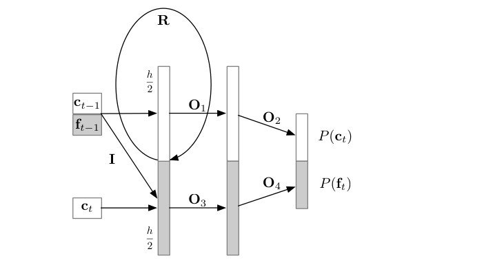
Figure 1. The architecture of the WaveRNN with the dual softmax layer. c represents the coarse (high 8-bits) of the sample and f represents the fine (low 8-bits) of the sample. The multiplication by R happens for both the coarse and fine bits simultaneously, then output of the gates is evaluated for the coarse bits only and c_t is sampled. Once c_t has been sampled from P(c_t), the gates are evaluated for the fine bits and f_t is sampled.

图 1. 带双 softmax 层的 WaveRNN 结构。c 表示采样点的粗分量（高 8 位），f 表示精细分量（低 8 位）。乘以 R 对粗、精位同时进行，然后只对粗位计算各门的输出并采样 c_t。一旦从 P(c_t) 中采出 c_t，再对精细位计算各门并采样 f_t。

We split the state of the RNN in two parts that predict respectively the 8 coarse (or more significant) bits c_t and the 8 fine (or least significant) bits f_t of the 16-bit audio sample (Figure 1). Each part feeds into a softmax layer over the corresponding 8 bits and the prediction of the 8 fine bits is conditioned on the 8 coarse bits. The resulting Dual Softmax layer allows for efficient prediction of 16-bit samples using two small output spaces (2^8 values each) instead of a single large output space (with 2^{16} values). Figure 1 shows this visually. We note that it is possible to train with one softmax over all 2^{16} values, but that in addition to requiring significantly more parameters, memory and compute, it consistently performs 1-2 centi-nats worse.

我们把 RNN 的状态分成两部分，分别预测 16 位音频采样的 8 个粗（更重要的）位 c_t 和 8 个精细（最不重要的）位 f_t（图 1）。每一部分都送入对应 8 位上的 softmax，并且精细 8 位的预测条件于粗 8 位。由此得到的双 Softmax 层可以用两个较小的输出空间（各 2^8 个取值）来高效预测 16 位采样，而不必用一个很大的输出空间（2^{16} 个取值）。图 1 给出了直观示意。需要说明，也可以用覆盖全部 2^{16} 个取值的单个 softmax 来训练，但除了参数、内存和计算明显更多之外，成绩还一律要差 1–2 个百分纳特。

2.1. WaveRNN Sampling on GPU

2.1. 在 GPU 上做 WaveRNN 采样

The above architecture reduces the number of operations N that are needed for each step from N = 60 for WaveNet with the 16-bit Discretized Logistic Mixture (DLM) output (Salimans et al., 2017) to N = 5 for the proposed WaveRNN with the dual softmax. Despite the reduced number of operations N, a regular implementation of WaveRNN sampling does not directly yield a real-time or faster synthesis. On a GPU the primary hindrance is not the raw FLOPs required for sampling; rather, the difficulties are twofold: limits on the memory bandwidth and the time that it takes to launch each of the N operations. Regarding the former, a WaveRNN with a state of 896 units (WaveRNN-896) has about 3M parameters. A regular implementation of sampling that calls each WaveRNN operation separately in sequence for each of the 24,000 samples loads all of the WaveRNN parameters from memory into the GPU registers during each step, totalling about 3e6 × 24e3 × 4 = 288 GBytes of required memory bandwidth. This is already more than a third of the memory bandwidth available in an Nvidia P100 GPU, giving by itself an upper bound of 3× real time for a regular implementation of sampling.

上述结构把每步所需运算次数 N，从带 16 位离散逻辑斯蒂混合（DLM）输出的 WaveNet 的 N = 60（Salimans et al., 2017），降到带双 softmax 的 WaveRNN 的 N = 5。尽管 N 已经减小，常规的 WaveRNN 采样实现并不能直接给出实时或更快的合成。在 GPU 上，主要障碍并不是采样所需的原始浮点运算次数；困难有两方面：内存带宽的限制，以及启动这 N 个运算各自所需的时间。就前者而言，状态为 896 个单元的 WaveRNN（WaveRNN-896）大约有 3M 参数。若按常规实现，对 24,000 个采样点中的每一个都依次单独调用各 WaveRNN 运算，则每一步都要把全部参数从内存载入 GPU 寄存器，总共大约需要 3e6 × 24e3 × 4 = 288 GB 的内存带宽。这已经超过 Nvidia P100 GPU 可用带宽的三分之一，单凭这一点，常规采样实现的上限就只有 3 倍实时。

The overhead of launching each operation separately on the GPU is even larger. While launching an operation on the GPU has a constant overhead of 5 microseconds, each step requires N = 5 such operations, which means the launch overhead alone induces an upper bound of 40,000 samples per second. For the WaveNet architecture, which requires (at least) N = 60 operations per sample, the launch overhead induces an upper bound of 3,300 samples per second. This is without considering the time spent on the actual computation of the operations. In practice a regular implementation of sampling in e.g. Tensorflow yields, respectively, about 1600 and 170 samples per second for WaveRNN-896 and for WaveNet.

在 GPU 上分别启动每一个运算的开销甚至更大。启动一次 GPU 运算有 5 微秒的固定开销，而每一步需要 N = 5 次这样的运算，这意味着仅启动开销就把上限压在每秒 40,000 个采样点。对 WaveNet 而言，每个采样点至少需要 N = 60 次运算，启动开销给出的上限是每秒 3,300 个采样点。这里还没有计入运算本身的计算时间。实践中，用例如 Tensorflow 做常规采样实现，WaveRNN-896 和 WaveNet 大约分别只有每秒 1600 和 170 个采样点。

We reduce both of these factors by implementing the sampling procedure directly as a single persistent GPU operation. The memory bandwidth bottleneck is avoided since the parameters are loaded only once into the GPU registers at the start of sampling and persist in the registers throughout the process. This is possible because the P100 GPU has 3.67M full-precision registers that suffice to store more than 7 million half-precision parameters, i.e. more than twice as many as needed in the WaveRNN-896. The operation launch bottleneck is also avoided, since the entire sampling process for an utterance is executed as a single GPU operation.

我们把采样过程直接实现成一次持续的 GPU 运算，从而同时压低这两个因素。内存带宽瓶颈被避开了，因为参数只在采样开始时载入 GPU 寄存器一次，并在整个过程中留在寄存器里。这之所以可行，是因为 P100 GPU 有 3.67M 个全精度寄存器，足以存放超过 700 万个半精度参数，也就是 WaveRNN-896 所需的两倍还多。运算启动的瓶颈也被避开了，因为整句语音的采样过程是作为一次 GPU 运算执行的。

A state size of 896 is chosen specifically to fit the P100 GPU which has 56 multi-processors. The minimum numbers of warps that must be assigned to each multi-processor to access the full register file of the GPU is 8. If we assign each warp to a state calculation, then the state size must be a multiple of 56 ∗ 8 = 448 and the largest multiple that fits in the available register space is 896.

状态宽度取 896，是专门为有 56 个多处理器的 P100 GPU 选定的。要访问 GPU 的全部寄存器堆，每个多处理器至少要分配 8 个 warp。若把每个 warp 分给一次状态计算，则状态宽度必须是 56 ∗ 8 = 448 的倍数，而能装进可用寄存器空间的最大倍数正是 896。

The resulting GPU kernel for WaveRNN sampling is two orders of magnitude more efficient than the regular sampling implementation, reaching 96,000 samples/second for the WaveRNN-896. The corresponding operation for WaveNet reaches 8,000 samples/second. The new overhead d(op) is now given by the synchronization of the thousands of cores in the GPU (Xiao & c. Feng, 2010), which takes just 500 nanoseconds per synchronization, instead of the 5 microseconds needed for each operation launch.

由此得到的 WaveRNN 采样 GPU 内核，比常规采样实现高效两个数量级，WaveRNN-896 可达到每秒 96,000 个采样点。对应的 WaveNet 运算达到每秒 8,000 个采样点。新的开销 d(op) 现在来自 GPU 中数千个核心的同步（Xiao & c. Feng, 2010），每次同步只需 500 纳秒，而不是每次启动运算所需的 5 微秒。

3. Sparse WaveRNN

3. 稀疏 WaveRNN

The WaveRNN architecture dramatically reduces the number of required operations N and implementing sampling as a single GPU operation eliminates much of the original computation c(op_i) and overhead d(op_i) bottlenecks. We next present a technique for reducing directly the amount of computation c(op_i) required by each operation. Decreasing the number of hidden units will reduce the amount of computation, but this comes with a significant loss in quality (Table 3). Instead, we reduce the number of non-zero weights in the network by sparsifying the weight matrices while retaining a large state size and respective representation capacity. This reduces c(op_i) since the number of non-zero weights is directly proportional to c(op_i) (Table 4).

WaveRNN 结构大幅减少了所需运算次数 N，把采样做成一次 GPU 运算，又消除了原先计算 c(op_i) 和开销 d(op_i) 中的很大一部分瓶颈。接下来我们给出一种直接降低每次运算所需计算量 c(op_i) 的技术。减少隐单元数会降低计算量，但质量会明显下降（表 3）。我们转而在保持较大状态宽度及相应表示能力的同时，把权重矩阵稀疏化，从而减少网络中的非零权数量。由于非零权数量与 c(op_i) 成正比，这样做会降低 c(op_i)（表 4）。

3.1. Weight Sparsification Method

3.1. 权重稀疏化方法

We use a pruning scheme based on the weight magnitude that increases sparsity as training proceeds (Narang et al., 2017a; Zhu & Gupta, 2017). We maintain a binary mask specifying the sparsity pattern of weight matrices. At the beginning of training, the weight matrices are dense. Every 500 steps, the weights within each sparsified layer are sorted by their magnitude and the mask is updated by zeroing out k weights with the smallest magnitude. The number k is computed as a fraction z of the total number of weights, which is gradually increased from 0 to the target sparsity Z as a function of the training step t:

我们采用基于权重大小的剪枝方案，并在训练过程中逐步提高稀疏度（Narang et al., 2017a; Zhu & Gupta, 2017）。我们维护一个二值掩码，用来指定权重矩阵的稀疏模式。训练开始时，权重矩阵是稠密的。每 500 步，把每个被稀疏化层中的权重按大小排序，并把幅值最小的 k 个权重在掩码中置零。k 取为总权数量的一个比例 z，而 z 随训练步数 t 从 0 逐渐增到目标稀疏度 Z：

z = Z [ 1 − (1 − (t − t_0)/S )^3 ]

where t_0 is the step at which weight pruning begins and S is the total number of pruning steps. We use t_0 = 1000, S = 200k and train for a total of 500k steps for all models. Such a scheme is practical, easy to integrate into existing models, and does not increase the training time. We sparsify the three gate matrices within the GRU cell separately.

其中 t_0 是开始做权重剪枝的步数，S 是剪枝的总步数。对所有模型，我们取 t_0 = 1000、S = 200k，并总共训练 500k 步。这一方案实用，也容易接到已有模型里，并且不会增加训练时间。我们把 GRU 单元里的三个门矩阵分别稀疏化。

3.2. Structured Sparsity

3.2. 结构化稀疏

We need to encode the sparsity mask in a manner that allows for efficient computation. The standard Compressed Sparse Row format uses about the same amount of storage for encoding the sparsity mask as it does for storing the parameters. Unlike hardware-oriented approaches such as Viterbi pruning (Lee et al., 2018), we explore structured sparsity as a means for reducing memory overhead. The structure in the sparsity mask that we consider is in the form of non-overlapping blocks of weights which are pruned or retained together based on the average magnitude of the weights within the block. We find that blocks of m = 16 weights lose little performance over unstructured sparsity while reducing the amount of memory needed for storing the sparsity pattern to 1/m of that required by an unstructured mask. Besides rectangular 4 × 4 blocks that we found to work well (Gray et al., 2017; Narang et al., 2017b), we also adopt blocks of shape m × 1 that induce an even lower memory bandwidth overhead. In the case of m × 1 blocks one only needs to retrieve a single activation value from the hidden state to perform the dot product. This is in contrast with the square blocks where for each block one needs to retrieve 4 activation values from the hidden state. We report results for both 16 × 1 and 4 × 4 blocks. The benchmarks confirm the greater speed of the 16 × 1 blocks (Table 4).

稀疏掩码需要用便于高效计算的方式来编码。标准的压缩稀疏行格式，用来编码掩码的存储量大约和存储参数本身相当。与面向硬件的做法（例如 Viterbi 剪枝，Lee et al., 2018）不同，我们探索用结构化稀疏来降低内存开销。我们所考虑的掩码结构，是互不重叠的权重块：根据块内权重的平均幅值，整块一起剪掉或保留。我们发现，大小为 m = 16 的块相对非结构化稀疏几乎不损失性能，却把存储稀疏模式所需的内存降到非结构掩码的 1/m。除了我们觉得效果较好的矩形 4 × 4 块（Gray et al., 2017; Narang et al., 2017b）之外，我们还采用 m × 1 形状的块，其内存带宽开销更低。对 m × 1 块，做点积时只需从隐状态里取一个激活值。这与方形块不同：每个块都要从隐状态里取 4 个激活值。我们同时报告 16 × 1 和 4 × 4 块的结果。基准测试证实 16 × 1 块更快（表 4）。

3.3. Sparse WaveRNN Sampling on Mobile CPU

3.3. 在手机 CPU 上做 Sparse WaveRNN 采样

We take advantage of the low computation and memory bandwidth required by Sparse WaveRNN to implement matrix-vector operations necessary for sampling on mobile CPU. To maximize memory utilization, weights are stored in 16-bit floating point and converted to 32-bit floating point before being used in the computation. The activations and the calculations are kept in 32-bit floating point. The low memory overhead afforded by small blocks allows the sparse matrix-vector products to match the performance of dense matrix-vector products with the same parameter count. The number of sequential matrix-vector products per second is thus determined almost entirely by the number of parameters in the network.

我们利用 Sparse WaveRNN 所需计算和内存带宽较低这一点，在手机 CPU 上实现采样所需的矩阵–向量运算。为尽量提高内存利用率，权重以 16 位浮点存储，计算前再转成 32 位浮点。激活值和计算过程保持 32 位浮点。小块带来的低内存开销，使稀疏矩阵–向量乘能够达到与同等参数量的稠密矩阵–向量乘相当的性能。于是，每秒可做的顺序矩阵–向量乘次数，几乎完全由网络中的参数量决定。

4. Subscale WaveRNN

4. 子尺度 WaveRNN

We have described two ways of reducing sampling time in high-fidelity audio generation: the WaveRNN that reduces N and d(op) and the Sparse WaveRNN that reduces N and c(op). Lastly we reduce the contribution from the factor |u| in Equation 1. This factor depends on the size of the utterance u and a direct reduction of the size of u itself (such as going from 16 to 8 bits per sample) would negatively affect audio quality. Instead, we propose a method for generating a batch of B samples per step, instead of just one:

我们已经介绍了两种缩短高保真音频生成采样时间的办法：WaveRNN 降低 N 和 d(op)，Sparse WaveRNN 降低 N 和 c(op)。最后，我们降低 (1) 式中 |u| 这一因子的贡献。这一因子取决于语句 u 的长度，若直接缩小 u 本身（例如从每采样点 16 位降到 8 位）会损害音质。我们转而提出一种每步生成一批 B 个采样点、而不是只生成一个的方法：

T(u) = (|u|/B) Σ_{i=1}^{N} (c(op_i^B) + d(op_i^B)) (3)

In many cases, the computation time for a batch of B examples, c(op_i^B), grows sublinearly in the computation time of a single example c(op_i) because weights are reused and spare computational capacity is available. The ability to batch samples also makes it possible to generate across multiple processors and have a reduction in total sampling time that is linear in the number of processors.

在许多情形下，一批 B 个样本的计算时间 c(op_i^B) 相对单个样本的计算时间 c(op_i) 是次线性增长的，因为权重可以复用，并且还有闲置的计算能力。能够把采样点打成批次，也使得可以跨多个处理器生成，从而让总采样时间随处理器数目线性下降。

Previous work on producing more than one sample per step in sequential models has required breaking local dependencies (Reed et al., 2017): two nearby samples that strongly depend on each other are produced independently, possibly conditioned on other samples. We introduce a general method that allows us to trade a small constant number of distant past and future dependencies for the ability to generate batches of B samples per step.

先前在序列模型里每步产出多于一个采样点的工作，往往需要切断局部依赖（Reed et al., 2017）：两个彼此强烈依赖的邻近采样点被独立生成，顶多再条件于别的采样点。我们引入一种通用方法，用少量、数目固定的较远过去和未来依赖，来换取每步生成一批 B 个采样点的能力。

4.1. Subscale Dependency Scheme

4.1. 子尺度依赖方案

From the tensor u one first extracts a set of B sub-tensors that have a frequency or scale that is B times smaller. Each sub-tensor corresponds to a subscale slice of u (see Figure 3). If u is a 24kHz audio utterance and B is 16, then each sub-tensor corresponds to a 24/16=1.5 kHz utterance. This is in contrast with a multi-scale scheme where the different subtensors extracted from u have increasing scales. Subscaling induces the following ordering on the dependencies of the variables in u, which is equivalent to the standard factorization of the joint:

首先从张量 u 中抽出 B 个子张量，它们的频率或尺度比原来小 B 倍。每个子张量对应 u 的一个子尺度切片（见图 3）。若 u 是 24 kHz 的语音，B 为 16，则每个子张量对应 24/16=1.5 kHz 的语句。这与多尺度方案不同：后者从 u 抽出的各个子张量尺度是递增的。子尺度在 u 中各变量的依赖上诱导出如下顺序，它与联合分布的标准分解是等价的：

P(u) = Π_{s=0}^{B} Π_{i=0}^{|u|/B} P( u_{Bi+s} | u_{Bj+s} for j < i, u_{Bk+z} for z < s and k ≥ 0 ) (4)

The sample u_{Bi+s} for a given (i, s) depends on all samples u_{Bk+z} for z < s and k ≥ 0. Generation of u proceeds as follows: one first generates the first sub-tensor, then the second sub-tensor conditioned on the first one, then the third sub-tensor conditioned on the previous two, etc. The Subscale WaveRNN that generates a given sub-tensor is conditioned on the future context of previous sub-tensors using a masked dilated CNN with relus and the mask applied over past connections instead of future ones. Like the multi-scale scheme, subscale schemes are equally applicable to multi-dimensional tensors.

对给定的 (i, s)，采样点 u_{Bi+s} 依赖于所有满足 z < s 且 k ≥ 0 的采样点 u_{Bk+z}。生成 u 的过程如下：先生成第一个子张量，再生成条件于第一个的第二个子张量，再生成条件于前两个的第三个子张量，依此类推。生成某个子张量的 Subscale WaveRNN，借助带 relu、并且把掩码加在过去连接而不是未来连接上的掩码膨胀 CNN，来条件于先前子张量的未来上下文。与多尺度方案一样，子尺度方案同样适用于多维张量。

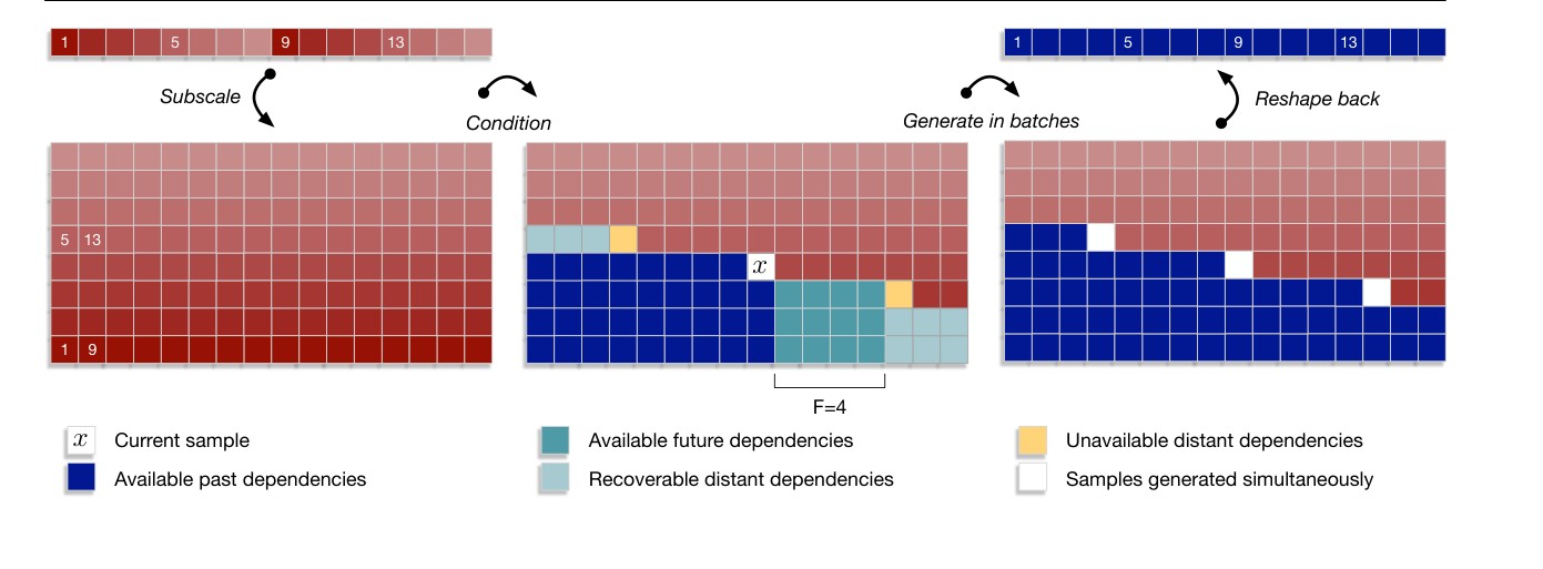
Figure 3. The dependency scheme of Subscale WaveRNN. Each box corresponds to one 16-bit sample. Subscaling first reshapes the tensor into B sub-tensors of interleaving samples. Then each sub-tensor is generated conditioned on past and future samples of previously generated sub-tensors; the past horizon is unbounded, whereas the future horizon of size F is tied to the receptive field of the conditioning network. Batched sampling can then be applied. The final tensor in the original scale is reconstituted from the generated sub-tensors.

图 3. Subscale WaveRNN 的依赖方案。每个方格对应一个 16 位采样点。子尺度首先把张量重排成 B 个由交错采样点组成的子张量。然后每个子张量在条件于先前已生成子张量的过去和未来采样点之后再生成；过去视野没有上界，而大小为 F 的未来视野则与条件网络的感受野绑定。随后即可做批量采样。最后再由生成的子张量重建出原来尺度上的张量。

4.2. Batched Sampling

4.2. 批量采样

In contrast to the multi-scale scheme, subscaling makes it possible to generate B samples in a single step. In Equation 4, for values of k > i + F for some future horizon F, the dependencies of u_{Bi+s} on future samples u_{Bk+z} with z < s become overwhelmingly weak (Figure 3). The conditioning network itself in the Subscale WaveRNN only sees a finite and usually small number of future samples from the previous sub-tensors. The sampling of a sub-tensor can begin immediately after the first F samples of the previous sub-tensor have been generated. Because the Subscale WaveRNN is shared across all sub-tensors, it is possible to batch inputs and after B ∗ F steps the total batch of the Subscale WaveRNN is B. Since the value of F (usually 64 or 128) is relatively small compared to the scale and length of u, even for relatively large values of B such as 16, the total lag of B ∗ F steps remains negligible for the total sampling latency. Although the conditioning network needs to be executed for each batch of samples, computing the conditioning network doesn’t affect the factor N of the Subscale WaveRNN because the network can be executed in parallel for a chosen number L of future samples. This increases the total sampling lag by B ∗ L steps, which even for values of L = 100 remains negligible. Due to batched sampling even our regular implementation in Tensorflow achieves just about real-time speed (24,000 samples/second) for a Subscale WaveRNN 16× with 1024 hidden state units.

与多尺度方案不同，子尺度使得可以在单步内生成 B 个采样点。在 (4) 式中，对某个未来视野 F，当 k > i + F 时，u_{Bi+s} 对满足 z < s 的未来采样点 u_{Bk+z} 的依赖会变得极弱（图 3）。Subscale WaveRNN 里的条件网络本身，从先前子张量里只能看到有限、通常也较少的未来采样点。一旦前一个子张量的前 F 个采样点已经生成，就可以立刻开始对当前子张量采样。由于 Subscale WaveRNN 在所有子张量上共享，可以把输入打成批次；经过 B ∗ F 步之后，Subscale WaveRNN 的总批大小就是 B。F 的取值（通常是 64 或 128）相对 u 的尺度和长度较小，因此即便 B 大到 16，B ∗ F 步的总滞后对整体采样延迟仍然可以忽略。虽然每批采样点都要执行条件网络，但计算条件网络并不影响 Subscale WaveRNN 的因子 N，因为该网络可以对选定数量 L 的未来采样点并行执行。这会把总采样滞后再增加 B ∗ L 步，即便 L = 100，也仍然可以忽略。由于可以批量采样，即便我们用常规 Tensorflow 实现，带 1024 个隐状态单元的 Subscale WaveRNN 16× 也能达到几乎实时的速度（每秒 24,000 个采样点）。

4.3. Recovering Future and Past Dependencies

4.3. 恢复未来和过去的依赖

Dropping distant future dependencies for k > i + F allows us in principle also to recover an almost equal number of distant past dependencies. A sub-tensor z that succeeds the current sub-tensor s is (z − s)(F + 1) steps behind s, but leaves a trace of distant past samples. During training and sampling these distant past samples can be accessed to condition the generation of the current pass s. Analogously, a constant number of future distant samples beyond i + F from sub-tensors previous to s are also available for additional conditioning. The exact dependency scheme of using subscaling and batched sampling includes these distant dependencies; in practice, however, choosing a larger value F appears simpler than embedding the distant dependencies.

丢掉 k > i + F 那些较远的未来依赖，原则上也让我们可以恢复几乎同样数量的较远过去依赖。排在当前子张量 s 之后的子张量 z，比 s 落后 (z − s)(F + 1) 步，但会留下一串较远的过去采样点。在训练和采样时，可以取用这些较远的过去采样点，来条件当前这一轮 s 的生成。类似地，在 i + F 之外、来自 s 之前那些子张量的、数目固定的较远未来采样点，也可以用来做额外的条件。使用子尺度和批量采样的精确依赖方案包含这些较远依赖；不过在实践中，把 F 取得更大，看起来比把这些较远依赖嵌进模型更简单。

4.4. Fused Subscale WaveRNN

4.4. 融合的 Subscale WaveRNN

We use the scheme behind the Subscale WaveRNN to directly generate more than 16 bits per step in the WaveRNN itself. We take a Subscale WaveRNN 2× model and instead of batching the 2 sub-tensors we split the hidden state of the WaveRNN in two parts. We then use 8 softmaxes of 4 bits each and an F value of just two. The samples from the sub-tensors are given directly to the WaveRNN as input without using a conditioning network. The resulting Fused Subscale WaveRNN 2× achieves only a small drop in the quality of the output (Table 3), but maps well onto the WaveRNN GPU custom operation. Compared to WaveRNN which runs at 4× real time, this model generates 32 bits per step and requires fewer synchronizations, resulting in a sampling speed of 10× real time. We note that in contrast to the Subscale WaveRNN, because fusion requires splitting the hidden state, audio quality drops quickly for factors beyond 2× in the Fused Subscale WaveRNN.

我们把 Subscale WaveRNN 背后的方案直接用到 WaveRNN 内部，使每步生成超过 16 位。我们取一个 Subscale WaveRNN 2× 模型，不是把 2 个子张量打成批次，而是把 WaveRNN 的隐状态分成两部分。然后使用 8 个各覆盖 4 位的 softmax，并把 F 取为只有 2。子张量中的采样点直接作为输入送给 WaveRNN，不再使用条件网络。由此得到的融合 Subscale WaveRNN 2×，输出质量只下降一点点（表 3），但能很好地映射到 WaveRNN 的定制 GPU 运算上。相比以 4 倍实时运行的 WaveRNN，这一模型每步生成 32 位，所需同步也更少，采样速度达到 10 倍实时。需要说明的是，与 Subscale WaveRNN 不同，融合需要拆分隐状态，因而在融合 Subscale WaveRNN 里，因子超过 2× 时音质会下降得很快。

5. Experiments

5. 实验

We perform experiments on the text-to-speech synthesis task and report the quality evaluation results as well as the sampling speed of our benchmarks on the corresponding platforms.

我们在文本转语音任务上做实验，并报告质量评价结果，以及在相应平台上基准测试的采样速度。

Text-to-speech models were trained on a dataset of 44 hours of North American English speech recorded by a professional speaker (van den Oord et al., 2017). The generation is conditioned on conventional linguistic features and predicted pitch information. All compared models synthesize raw audio at 24 kHz in 16-bit format. The evaluation is carried out on a held-out test set where we consider three performance measures: Negative Log-Likelihood of ground-truth audio; MOS between 1 (Bad) and 5 (Excellent) of generated speech utterances according to the subjective quality evaluation by human raters; and the results of direct A/B comparison tests between pairs of models as rated subjectively by humans on a scale between -3 (Much Worse Than) and +3 (Much Better Than).

文本转语音模型在一套由专业发音人录制、共 44 小时的北美英语语音数据上训练（van den Oord et al., 2017）。生成时条件于常规语言学特征和预测得到的音高信息。所有比较的模型都以 24 kHz、16 位格式合成原始音频。评价在留出的测试集上进行，我们考虑三项指标：相对真值音频的负对数似然；由评分人对生成语句做主观质量评价得到的、介于 1（差）和 5（优秀）之间的 MOS；以及成对模型的直接 A/B 比较，由人按 -3（差得多）到 +3（好得多）的量表主观评分。

5.1. WaveRNN Quality Evaluation & Speed

5.1. WaveRNN 的质量评价与速度

The WaveRNN models are trained on sequences of 960 audio samples of 16-bit each and full back-propagation-through-time is applied to the models. Table 3 reports the results for various sizes of WaveRNN. The larger WaveRNNs approach the NLL performance of the 60-layer WaveNet model. A human rated A/B comparison test between WaveRNN-896 and WaveNet indicates no significant difference in the quality of the speech produced (Table 1). An additional A/B comparison test between WaveNet and WaveRNN-2048 also shows no significant differences.

WaveRNN 模型在每条 960 个 16 位音频采样点的序列上训练，并做完整的沿时间反向传播。表 3 报告了不同规模 WaveRNN 的结果。更大的 WaveRNN 在 NLL 上已经接近 60 层 WaveNet。WaveRNN-896 与 WaveNet 之间由人工评分的 A/B 比较表明，合成语音的质量没有显著差异（表 1）。WaveNet 与 WaveRNN-2048 的另一组 A/B 比较同样没有显著差异。

The persistent GPU operations that we implement are most efficient for the WaveRNN-896 model, which achieves a NLL of 5.42 and a MOS value of 4.37 ± 0.07. Samples are generated at 96,000 samples per second for a batch size of 1 and 39,000 samples per second for a batch size of 4.

我们实现的持续 GPU 运算对 WaveRNN-896 最为高效，该模型的 NLL 为 5.42，MOS 为 4.37 ± 0.07。批大小为 1 时，采样速度为每秒 96,000 个采样点；批大小为 4 时为每秒 39,000 个采样点。

Model (vs WaveRNN-896)	Better	Neutral	Worse	Overall	Significant
WaveNet 512 (60)	145	529	126	0.02 ± 0.08	No
Sparse WR 384 (2048/96.4%)	139	441	220	−0.14 ± 0.08	Yes
Sparse WR Mobile	71	456	273	−0.40 ± 0.09	Yes
Subscale WR 1024 (16×)	113	558	129	−0.03 ± 0.05	No

模型（相对 WaveRNN-896）	更好	中性	更差	总体	显著
WaveNet 512 (60)	145	529	126	0.02 ± 0.08	否
Sparse WR 384 (2048/96.4%)	139	441	220	−0.14 ± 0.08	是
Sparse WR Mobile	71	456	273	−0.40 ± 0.09	是
Subscale WR 1024 (16×)	113	558	129	−0.03 ± 0.05	否

Table 1. Results of A/B comparison tests between a given model and the WaveRNN-896. Each test includes 800 human ratings with grades between -3 (Much Worse Than) and 3 (Much Better Than). We collapse the counts for the different positive and negative categories.

表 1. 给定模型与 WaveRNN-896 的 A/B 比较结果。每次测试包含 800 条人工评分，分数介于 -3（差得多）和 3（好得多）之间。我们把不同的正向和负向类别计数合并在一起。

Size	Sparsity %	Type	Platform	Samples/sec
512	95%	4×4	SD 835	29,100
512	95%	4×4	SD 808	19,800
512	95%	16×1	SD 835	31,400
512	95%	16×1	SD 808	21,600

规模	稀疏度 %	类型	平台	采样点/秒
512	95%	4×4	SD 835	29,100
512	95%	4×4	SD 808	19,800
512	95%	16×1	SD 835	31,400
512	95%	16×1	SD 808	21,600

Table 2. Benchmarks for Sparse WaveRNN Mobile sampling performance executed on the widely available Snapdragon 808 and 835 mobile CPUs. The model has 1024 hidden units, 95% sparsity and 4 × 4 structure sparsity. The benchmarks are based on running an equivalent computation on the mobile CPU including layers and softsign non-linearities (Section 5.2).

表 2. Sparse WaveRNN Mobile 在广泛使用的骁龙 808 和 835 手机 CPU 上的采样性能基准。该模型有 1024 个隐单元，稀疏度为 95%，并采用 4 × 4 结构稀疏。基准是在手机 CPU 上运行等价计算得到的，包括各层以及 softsign 非线性（第 5.2 节）。

Model	NLL	MOS
WaveNet	5.29	4.51 ± 0.08
WaveRNN 224	5.67	3.73 ± 0.09
WaveRNN 384	5.56	4.23 ± 0.09
WaveRNN 896	5.42	4.37 ± 0.07
WaveRNN 2048	5.33	4.46 ± 0.07
Sparse WR Mobile	5.52	4.33 ± 0.08
Sparse WR 224 / 1536@97.8%	5.48	4.39 ± 0.07
Sparse WR 384 / 2048@96.4%	5.42	4.48 ± 0.07
Subscale WR 1024 (16×)	5.52	4.30 ± 0.08
Subscale WR 1024 (8×)	5.46	4.39 ± 0.06
Fused Subscale WR 896 (2×)	5.45	4.31 ± 0.08

模型	NLL	MOS
WaveNet	5.29	4.51 ± 0.08
WaveRNN 224	5.67	3.73 ± 0.09
WaveRNN 384	5.56	4.23 ± 0.09
WaveRNN 896	5.42	4.37 ± 0.07
WaveRNN 2048	5.33	4.46 ± 0.07
Sparse WR Mobile	5.52	4.33 ± 0.08
Sparse WR 224 / 1536@97.8%	5.48	4.39 ± 0.07
Sparse WR 384 / 2048@96.4%	5.42	4.48 ± 0.07
Subscale WR 1024 (16×)	5.52	4.30 ± 0.08
Subscale WR 1024 (8×)	5.46	4.39 ± 0.06
Fused Subscale WR 896 (2×)	5.45	4.31 ± 0.08

Table 3. WaveRNN NLL and MOS results on the text-to-speech benchmark. The Sparse WaveRNN Mobile model has 1024 hidden units with a 95.2% sparsity ratio and 4×4 blocks.

表 3. 文本转语音基准上 WaveRNN 的 NLL 与 MOS。Sparse WaveRNN Mobile 模型有 1024 个隐单元，稀疏比为 95.2%，并采用 4×4 块。

5.2. Sparse WaveRNN Quality Evaluation & Speed

5.2. Sparse WaveRNN 的质量评价与速度

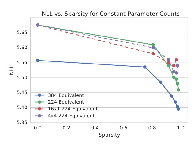
Figure 2. The Sparse WaveRNNs on each curve have the same number of parameters. The Sparse WaveRNNs with structured sparsity 16 × 1 and 4 × 4 hit a point of maximum performance at a high degree of sparsity. The points of maximum performance for the unstructured Sparse WaveRNNs fall beyond the tested range.

图 2. 每条曲线上的 Sparse WaveRNN 具有相同的参数量。采用 16 × 1 和 4 × 4 结构稀疏的 Sparse WaveRNN，在很高的稀疏度上达到性能最高点。非结构化 Sparse WaveRNN 的性能最高点则落在所测范围之外。

Figure 2 illustrates a core point about our investigation into sparse models. We use a dense WaveRNN model with a state size of 224 as a starting point because it is the largest that could be run on many current off the shelf mobile processors. As a second baseline we use a model with a state size of 384 that we estimate to still be out of reach for even the fastest mobile platforms, as the model would require 30 GB/sec of memory bandwidth and no current mobile platform can provide this amount.

图 2 说明了我们考察稀疏模型时的一个核心点。我们以状态宽度为 224 的稠密 WaveRNN 作为起点，因为它是许多现成手机处理器上能够跑起来的最大规模。作为第二条基线，我们使用状态宽度为 384 的模型：我们估计即便最快的移动平台也还跑不动它，因为该模型需要 30 GB/秒的内存带宽，而目前没有移动平台能提供这么多。

Figure 2 shows that if we fix the total parameter count – and keep the corresponding sampling time also the same – then as we increase the degree of sparsity and the resulting size of layers, the fidelity of the models improves. This holds up to high degrees of sparsity > 98%, where the state size h of the models reaches 2048 hidden units. Higher sparsity monotonically implies lower NLL and in fact higher sparsity levels have larger slopes. This suggests that for a given computational budget at inference time, it is much more efficient to use those parameters to sparsely connect a larger number of neurons in each layer.

图 2 表明：若固定总参数量——并把相应的采样时间也保持不变——那么随着稀疏度提高、层随之变大，模型的保真度也会提高。这一关系一直保持到高于 98% 的稀疏度，此时模型的状态宽度 h 达到 2048 个隐单元。更高的稀疏度单调地对应更低的 NLL，而且更高稀疏度上的斜率实际上更大。这表明，在给定的推断计算预算下，用这些参数在每一层里稀疏地连接更多神经元，要高效得多。

In Table 4 and Figure 2 we examine the impact of using block sparsity on NLL and speed, and find that 4 × 4 blocks generally yield the best NLL, but 16 × 1 blocks have a speed advantage. Surprisingly, both have better NLL than unstructured sparsity at low sparsity levels, but improve more slowly and eventually hit a minimum around 95% while unstructured sparsity continues to improve. We did not explore even higher levels of unstructured sparsity only because investigating extremely high levels of sparsity requires starting with extremely large dense layers making training computationally intensive. Unstructured sparsity is unsurprisingly slower during inference, but depending on the quality trade offs involved in using blocks (which will likely vary from model to model), it might still be preferred.

在表 4 和图 2 中，我们考察块稀疏对 NLL 和速度的影响，发现 4 × 4 块通常给出最好的 NLL，但 16 × 1 块在速度上占优。出人意料的是，在较低稀疏度时两者的 NLL 都好于非结构化稀疏，但提升更慢，并最终在大约 95% 处达到最低点，而非结构化稀疏仍在继续变好。我们没有再探更高的非结构化稀疏度，仅仅是因为考察极高稀疏度需要从极大的稠密层起步，训练会非常耗计算。非结构化稀疏在推断时更慢，这并不令人意外；不过，是否仍更倾向于它，取决于使用块时在质量上的取舍（这很可能因模型而异）。

To obtain an estimate of Sparse WaveRNN sampling speed, we benchmarked all computationally heavy operations (sparse matrix-vector multiplication and softsign non-linearity evaluations) required for producing each audio sample, and used these measurements to derive an estimate of the sampling speed. For example, a sample from a 1024 model requires 3 multiplications of 1024×1024 for the GRU gates, two multiplications of 512×512 for the projection, two multiplications of 512×256 for the logits and evaluating 3072 non-linearities. We add up the time for all of these operations to estimate the upper bound on sampling performance.

为估计 Sparse WaveRNN 的采样速度，我们对生成每个音频采样点所需的全部重计算运算（稀疏矩阵–向量乘和 softsign 非线性求值）做了基准测试，并用这些测量值推出采样速度的估计。例如，1024 模型的一个采样点需要 3 次 1024×1024 的乘法（用于 GRU 各门）、两次 512×512 的乘法（用于投影）、两次 512×256 的乘法（用于 logits），以及计算 3072 个非线性。我们把这些运算的时间加总，用来估计采样性能的上限。

We perform our benchmarks on the Snapdragon 808 (SD 808) and Snapdragon 835 (SD 835) mobile CPUs, which are widely available in mobile phones. The two big cores of the SD 808 at 1.8GHz can do 28.8 Gflops/sec and the bandwidth out of the shared L2 cache is 14.4 GB/sec. The SD 835 is faster at 2.35GHz, with 2 cores able to do 37.6 Gflops/sec and pull 18.8 GB/sec from the cache. In practice, the achievable flops are often much lower (geekbench, a;b) and around 14.4 Gflops/sec and 28.2 Gflops/sec for SD 808 and 835 respectively. These numbers suggest that both our dense and sparse implementations are close to the maximum possible performance of the processor (the limiting factor for all kernels is bandwidth and not flops). For comparison, a modern Intel desktop CPU with AVX2 can do over 200 Gflops/sec and get over 200 GB/sec of bandwidth out of the L2 cache with only two cores.

基准测试在骁龙 808（SD 808）和骁龙 835（SD 835）这两款广泛用于手机的 CPU 上进行。SD 808 的两个大核在 1.8 GHz 下可以达到 28.8 Gflops/秒，共享 L2 缓存的带宽是 14.4 GB/秒。SD 835 更快，主频 2.35 GHz，两核可以达到 37.6 Gflops/秒，并能从缓存中拉出 18.8 GB/秒。实践中可达到的浮点性能往往低得多（geekbench, a;b），SD 808 和 835 分别大约只有 14.4 和 28.2 Gflops/秒。这些数字表明，我们的稠密和稀疏实现都已经接近处理器可能达到的最高性能（所有内核的限制因素都是带宽而不是浮点运算）。作为比较，一颗带 AVX2 的现代英特尔桌面 CPU，只用两个核心就可以超过 200 Gflops/秒，并从 L2 缓存获得超过 200 GB/秒的带宽。

Size	Sparse %	Type	SD 808 GF	SD 808 MVM ×10^3	SD 835 GF	SD 835 MVM ×10^3
224	0	–	9.6	95.4	11.0	95.4
384	0	–	9.6	32.6	11.0	32.6
1024	0	–	3.8	1.8	8.0	3.8
512	80.0	1X1	2.1	20.1	3.8	36.5
1024	95.0	1X1	1.8	17.2	3.4	32.2
2048	96.4	1X1	2.0	6.5	3.7	12.1
512	80.0	4X4	8.9	85.2	14.3	136.6
1024	95.0	4X4	8.0	75.6	12.4	118.2
2048	96.4	4X4	8.5	28.1	12.8	42.2
512	80.0	16X1	9.8	94.0	14.5	138.1
1024	95.0	16X1	9.0	85.5	13.4	127.4
2048	96.4	16X1	9.0	30.0	12.6	41.8

规模	稀疏 %	类型	SD 808 GF	SD 808 MVM ×10^3	SD 835 GF	SD 835 MVM ×10^3
224	0	–	9.6	95.4	11.0	95.4
384	0	–	9.6	32.6	11.0	32.6
1024	0	–	3.8	1.8	8.0	3.8
512	80.0	1X1	2.1	20.1	3.8	36.5
1024	95.0	1X1	1.8	17.2	3.4	32.2
2048	96.4	1X1	2.0	6.5	3.7	12.1
512	80.0	4X4	8.9	85.2	14.3	136.6
1024	95.0	4X4	8.0	75.6	12.4	118.2
2048	96.4	4X4	8.5	28.1	12.8	42.2
512	80.0	16X1	9.8	94.0	14.5	138.1
1024	95.0	16X1	9.0	85.5	13.4	127.4
2048	96.4	16X1	9.0	30.0	12.6	41.8

Table 4. Performance of ARM matrix-vector multiplies (MVM) and respectively Gflops (GF) per second, using two big cores of each of the processors Snapdragon 808 and 835. For the dense 224 and 384 kernels, higher performance is possible (11.7 Gflops/sec and 16.3 Gflops/sec respectively) with custom layouts of the dense matrix, but this is best performance we could achieve with the standard row major layout.

表 4. 在骁龙 808 和 835 上各用两个大核时，ARM 矩阵–向量乘（MVM）以及相应每秒 Gflops（GF）的性能。对稠密的 224 和 384 内核，若对稠密矩阵采用定制布局，还可以更高（分别达到 11.7 和 16.3 Gflops/秒），但这是我们在标准行主序布局下能够达到的最好成绩。

5.3. Subscale WaveRNN Quality Evaluation

5.3. Subscale WaveRNN 的质量评价

The conditioning network of the Subscale WaveRNN is a masked dilated 1D CNN and has ten layers, convolutional kernels of size 3, 384 convolutional channels, and 768 residual channels. The conditioning CNN has 5 stages of increasing dilation, for a total future horizon of F = 128 blocks of 8 or 16 samples each. The Subscale WaveRNNs that we evaluate have 1024 units in their hidden state. We do not use recoverable distant dependencies.

Subscale WaveRNN 的条件网络是带掩码的膨胀一维 CNN，共十层，卷积核大小为 3，有 384 个卷积通道和 768 个残差通道。该条件 CNN 有 5 段递增的膨胀，总的未来视野为 F = 128 个块，每块 8 或 16 个采样点。我们评价的 Subscale WaveRNN，隐状态都是 1024 个单元。我们没有使用可恢复的较远依赖。

We evaluate the model for two values of B, 8 and 16. The Subscale WaveRNN with B = 8 generates 8 16-bit samples at once at each step, which corresponds to a 3 kHz signal. As shown in Table 3, the Subscale WaveRNN 8× achieves a MOS of 4.39. This is equivalent to the MOS of the baseline WaveRNN-896 and it shows the ability of the Subscale WaveRNN 8× to accurately learn the distribution under the modified dependency scheme. We also evaluate a Subscale WaveRNN with B = 16, which generates an interleaving signal at 1.5 kHz. As shown in Table 1, the audio fidelity of the Subscale WaveRNN 16× is not significantly different from that of the WaveRNN-896 and, by transitivity, that of Wavenet 512 (60). This is remarkable as audio generation with sequential models can be extremely sensitive to lost dependencies, especially local ones, and this quality result demonstrates the effectiveness of the subscale dependency scheme to preserve all the local dependencies that are the key to the high performance of sequential models.

我们在 B 取 8 和 16 时评价该模型。B = 8 的 Subscale WaveRNN 每步一次生成 8 个 16 位采样点，相当于 3 kHz 信号。如表 3 所示，Subscale WaveRNN 8× 的 MOS 为 4.39。这与基线 WaveRNN-896 的 MOS 相当，表明 Subscale WaveRNN 8× 能够在改过的依赖方案下准确地学习该分布。我们还评价了 B = 16 的 Subscale WaveRNN，它生成的是 1.5 kHz 的交错信号。如表 1 所示，Subscale WaveRNN 16× 的音质与 WaveRNN-896 没有显著差异，因而传递地看，也与 WaveNet 512 (60) 没有显著差异。这一点很可观，因为用序列模型生成音频时，对丢失的依赖（尤其是局部依赖）可以极为敏感；这一质量结果表明，子尺度依赖方案能够保住对序列模型高性能至关重要的全部局部依赖。

The ability to batch computation by a factor of 8 or 16 yields a large amount of flexibility. Batching can increase throughput from a single GPU device increasing the overall sampling speed. In addition, it makes it possible to generate from multiple devices at once, where the generated bits are sent one-way and online from each device to the next. Such a setup gives in principle a linear speed-up over the sampling speed of a single device. If a single pass of Subscale WaveRNN with B = 16 runs at 4× real time on a GPU, then on a connected rack of 16 GPUs the Subscale WaveRNN 16× can in principle gain an equivalent linear speed-up for a total sampling speed of 4 ∗ B = 64 times real time. Subscale WaveRNN can also be combined with Sparse WaveRNN and executed on a multi-core CPU gaining a speed-up proportional to the number of cores available.

能够按 8 或 16 的倍数把计算打成批次，会带来很大的灵活性。批处理可以提高单块 GPU 的吞吐，从而加快总体采样速度。此外，它也使得可以同时从多台设备上生成，生成的比特从每台设备单向、在线地送到下一台。这样的布置原则上可以相对单设备采样速度获得线性加速。若 B = 16 的 Subscale WaveRNN 在一块 GPU 上单次前向达到 4 倍实时，那么在由 16 块 GPU 连成的机架上，Subscale WaveRNN 16× 原则上可以再获得相应的线性加速，总采样速度达到 4 ∗ B = 64 倍实时。Subscale WaveRNN 也可以和 Sparse WaveRNN 结合，在多核 CPU 上运行，并获得与可用核心数成正比的加速。

6. Conclusion

6. 结论

We introduced the WaveRNN, a simple and powerful recurrent network for the sequential modeling of high fidelity audio, and we have demonstrated a high performance implementation of this model on GPUs. We have shown that large sparse models have much better quality than small dense models with the same number of parameters and we have written high performance block-sparse matrix-vector product operations to demonstrate that sampling time is proportional to parameter count. We then showed that high fidelity audio generation is now achievable on widely available low-power mobile CPUs. Finally, we introduced the subscale dependency scheme that lets sequential models generate many samples per step while preserving the output quality of the original model. The underlying ideas of the methods we introduce are not specific to audio, and the results of sparse models have implications for inference in all types of neural networks.

我们介绍了 WaveRNN：一种简单而有力的循环网络，用于对高保真音频做序列建模，并展示了这一模型在 GPU 上的高性能实现。我们表明，在参数量相同的情况下，大而稀疏的模型质量远好于小而稠密的模型，并编写了高性能的块稀疏矩阵–向量乘运算，以表明采样时间与参数量成正比。接着我们表明，高保真音频生成现在已经可以在广泛使用的低功耗手机 CPU 上实现。最后，我们介绍了子尺度依赖方案，使序列模型能够每步生成多个采样点，同时保持原模型的输出质量。这些方法背后的想法并不限于音频，稀疏模型的结果对各类神经网络的推断都有启示。

References

参考文献

Chung, J., Gülçehre, Ç., Cho, K., and Bengio, Y. Empirical evaluation of gated recurrent neural networks on sequence modeling. CoRR, abs/1412.3555, 2014.

Diamos, G., Sengupta, S., Catanzaro, B., Chrzanowski, M., Coates, A., Elsen, E., Engel, J., Hannun, A., and Satheesh, S. Persistent RNNs: Stashing recurrent weights on-chip. In ICML, pp. 2024–2033, 2016.

Engel, J. Optimizing RNNs with differentiable graphs, June 2016. URL https://svail.github.io/diff_graphs/.

Engel, J., Resnick, C., Roberts, A., Dieleman, S., Eck, D., Simonyan, K., and Norouzi, M. Neural audio synthesis of musical notes with wavenet autoencoders. CoRR, abs/1704.01279, 2017.

geekbench, 2018a. URL https://browser.geekbench.com/v4/cpu/6960655.

geekbench, 2018b. URL https://browser.geekbench.com/v4/cpu/6473830.

Gordon, A., Eban, E., Nachum, O., Chen, B., Wu, H., Yang, T.-J., and Choi, E. MorphNet: Fast & Simple Resource-Constrained Structure Learning of Deep Networks. ArXiv e-prints, November 2017.

Gray, S., Radford, A., and Kingma, D. Block-sparse gpu kernels, Dec 2017. URL https://blog.openai.com/block-sparse-gpu-kernels/.

Gu, J., Bradbury, J., Xiong, C., Li, V. O. K., and Socher, R. Non-autoregressive neural machine translation. CoRR, abs/1711.02281, 2017.

Kalchbrenner, N., Espeholt, L., Simonyan, K., van den Oord, A., Graves, A., and Kavukcuoglu, K. Neural machine translation in linear time. CoRR, abs/1610.10099, 2016.

Kalchbrenner, N., van den Oord, A., Simonyan, K., Danihelka, I., Vinyals, O., Graves, A., and Kavukcuoglu, K. Video pixel networks. In ICML, volume 70, pp. 1771–1779, 2017.

Lee, D., Ahn, D., Kim, T., Chuang, P. I., and Kim, J.-J. Viterbi-based pruning for sparse matrix with fixed and high index compression ratio. ICLR, 2018. URL https://openreview.net/forum?id=S1D8MPxA-.

Mehri, S., Kumar, K., Gulrajani, I., Kumar, R., Jain, S., Sotelo, J., Courville, A. C., and Bengio, Y. SampleRNN: an unconditional end-to-end neural audio generation model. CoRR, abs/1612.07837, 2016.

Narang, S., Diamos, E. E. G. F., and Sengupta, S. Exploring sparsity in recurrent neural networks. CoRR, abs/1704.05119, 2017a.

Narang, S., Undersander, E., and Diamos, G. F. Block-sparse recurrent neural networks. CoRR, abs/1711.02782, 2017b.

Reed, S. E., van den Oord, A., Kalchbrenner, N., Colmenarejo, S. G., Wang, Z., Chen, Y., Belov, D., and de Freitas, N. Parallel multiscale autoregressive density estimation. In ICML, volume 70, pp. 2912–2921, 2017.

Salimans, T., Karpathy, A., Chen, X., and Kingma, D. P. PixelCNN++: Improving the pixelcnn with discretized logistic mixture likelihood and other modifications. CoRR, abs/1701.05517, 2017.

Simon, I. and Oore, S. Performance RNN: Generating music with expressive timing and dynamics. https://magenta.tensorflow.org/performance-rnn, 2017.

van den Oord, A., Dieleman, S., Zen, H., Simonyan, K., Vinyals, O., Graves, A., Kalchbrenner, N., Senior, A., and Kavukcuoglu, K. WaveNet: A generative model for raw audio. CoRR, abs/1609.03499, 2016a.

van den Oord, A., Kalchbrenner, N., and Kavukcuoglu, K. Pixel recurrent neural networks. In ICML, volume 48, pp. 1747–1756, 2016b.

van den Oord, A., Li, Y., Babuschkin, I., Simonyan, K., Vinyals, O., Kavukcuoglu, K., van den Driessche, G., Lockhart, E., Cobo, L. C., Stimberg, F., Casagrande, N., Grewe, D., Noury, S., Dieleman, S., Elsen, E., Kalchbrenner, N., Zen, H., Graves, A., King, H., Walters, T., Belov, D., and Hassabis, D. Parallel WaveNet: Fast high-fidelity speech synthesis. CoRR, abs/1711.10433, 2017.

Vaswani, A., Shazeer, N., Parmar, N., Uszkoreit, J., Jones, L., Gomez, A. N., Kaiser, L., and Polosukhin, I. Attention is all you need. CoRR, abs/1706.03762, 2017.

Wang, Y., Skerry-Ryan, R. J., Stanton, D., Wu, Y., Weiss, R. J., Jaitly, N., Yang, Z., Xiao, Y., Chen, Z., Bengio, S., Le, Q. V., Agiomyrgiannakis, Y., Clark, R., and Saurous, R. A. Tacotron: A fully end-to-end text-to-speech synthesis model. CoRR, abs/1703.10135, 2017.

Wu, Y., Schuster, M., Chen, Z., Le, Q. V., Norouzi, M., Macherey, W., Krikun, M., Cao, Y., and al. Google’s neural machine translation system: Bridging the gap between human and machine translation. CoRR, abs/1609.08144, 2016.

Xiao, S. and c. Feng, W. Inter-block GPU communication via fast barrier synchronization. In 2010 IEEE International Symposium on Parallel Distributed Processing (IPDPS), pp. 1–12, 2010.

Zhu, M. and Gupta, S. To prune, or not to prune: exploring the efficacy of pruning for model compression. CoRR, abs/1710.01878, 2017.