WaveNet: A Generative Model for Raw Audio

WaveNet：一种原始音频生成模型

Aäron van den Oord, Sander Dieleman, Heiga Zen†, Karen Simonyan, Oriol Vinyals, Alex Graves, Nal Kalchbrenner, Andrew Senior, Koray Kavukcuoglu

{avdnoord, sedielem, heigazen, simonyan, vinyals, gravesa, nalk, andrewsenior, korayk}@google.com

Google DeepMind, London, UK; † Google, London, UK

Aäron van den Oord、Sander Dieleman、Heiga Zen†、Karen Simonyan、Oriol Vinyals、Alex Graves、Nal Kalchbrenner、Andrew Senior、Koray Kavukcuoglu

{avdnoord, sedielem, heigazen, simonyan, vinyals, gravesa, nalk, andrewsenior, korayk}@google.com

Google DeepMind，英国伦敦；† Google，英国伦敦

Abstract

摘要

This paper introduces WaveNet, a deep neural network for generating raw audio waveforms. The model is fully probabilistic and autoregressive, with the predictive distribution for each audio sample conditioned on all previous ones; nonetheless we show that it can be efficiently trained on data with tens of thousands of samples per second of audio. When applied to text-to-speech, it yields state-of-the-art performance, with human listeners rating it as significantly more natural sounding than the best parametric and concatenative systems for both English and Mandarin. A single WaveNet can capture the characteristics of many different speakers with equal fidelity, and can switch between them by conditioning on the speaker identity. When trained to model music, we find that it generates novel and often highly realistic musical fragments. We also show that it can be employed as a discriminative model, returning promising results for phoneme recognition.

本文提出 WaveNet，一种生成原始音频波形的深度神经网络。这个模型是完全概率化的自回归（autoregressive）模型，每个音频采样点的预测分布都以之前所有采样点为条件；尽管如此，我们表明它可以在每秒音频含数万个采样点的数据上高效训练。用于文本转语音（text-to-speech）时，它达到了最先进的水平：无论英语还是普通话，人类听者都认为它的声音比最好的参数式系统和拼接式系统明显更自然。单个 WaveNet 能以同等保真度捕捉许多不同说话人的特征，并可以通过以说话人身份为条件在他们之间切换。用它来建模音乐时，我们发现它能生成新颖且往往非常逼真的音乐片段。我们还表明，它可以用作判别模型，在音素识别上取得了有希望的结果。

1 Introduction

1 引言

This work explores raw audio generation techniques, inspired by recent advances in neural autoregressive generative models that model complex distributions such as images (van den Oord et al. 2016a; van den Oord et al. 2016b) and text (Józefowicz et al. 2016). Modeling joint probabilities over pixels or words using neural architectures as products of conditional distributions yields state-of-the-art generation.

这项工作探索原始音频的生成技术，灵感来自神经自回归生成模型近来的进展；这类模型已能建模图像（van den Oord et al. 2016a; van den Oord et al. 2016b）和文本（Józefowicz et al. 2016）等复杂分布。用神经网络架构把像素或词的联合概率建模为条件分布的乘积，取得了最先进的生成效果。

Remarkably, these architectures are able to model distributions over thousands of random variables (e.g. 64$\times$64 pixels as in PixelRNN (van den Oord et al. 2016a)). The question this paper addresses is whether similar approaches can succeed in generating wideband raw audio waveforms, which are signals with very high temporal resolution, at least 16,000 samples per second (see Fig. 1).

值得一提的是，这些架构能够建模数千个随机变量上的分布（例如 PixelRNN（van den Oord et al. 2016a）中的 64$\times$64 个像素）。本文要回答的问题是：类似的方法能否成功生成宽带原始音频波形？这类信号的时间分辨率非常高，每秒至少有 16,000 个采样点（见图 1）。

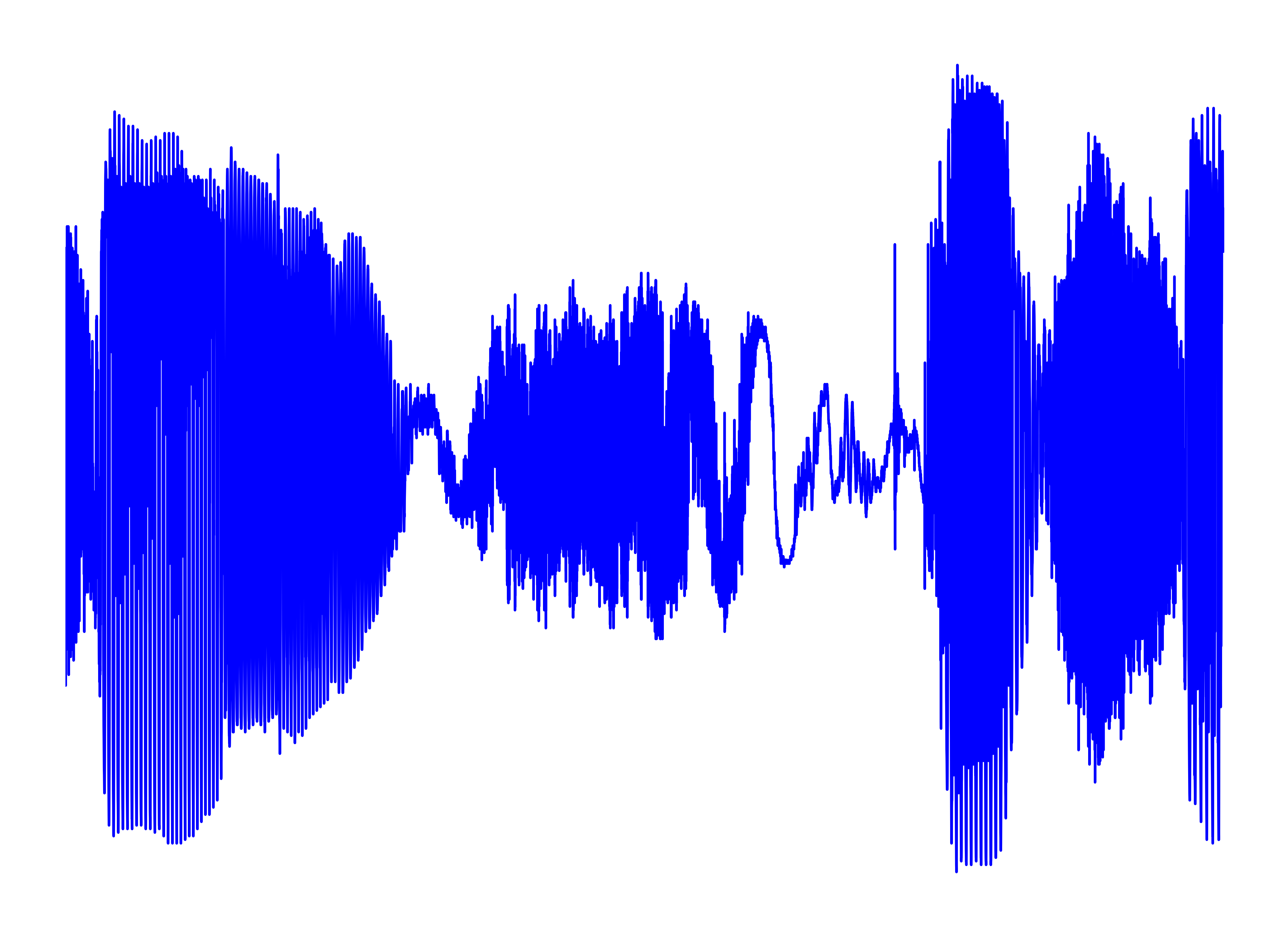
Figure 1: A second of generated speech.

图 1：一秒钟的生成语音。

This paper introduces WaveNet, an audio generative model based on the PixelCNN (van den Oord et al. 2016a; van den Oord et al. 2016b) architecture. The main contributions of this work are as follows:

本文提出 WaveNet，一个基于 PixelCNN（van den Oord et al. 2016a; van den Oord et al. 2016b）架构的音频生成模型。这项工作的主要贡献如下：

• We show that WaveNets can generate raw speech signals with subjective naturalness never before reported in the field of text-to-speech (TTS), as assessed by human raters.
• In order to deal with long-range temporal dependencies needed for raw audio generation, we develop new architectures based on dilated causal convolutions, which exhibit very large receptive fields.
• We show that when conditioned on a speaker identity, a single model can be used to generate different voices.
• The same architecture shows strong results when tested on a small speech recognition dataset, and is promising when used to generate other audio modalities such as music.

• 我们表明，经人类评分者评估，WaveNet 生成的原始语音信号在主观自然度上达到了文本转语音（TTS）领域此前从未报告过的水平。
• 为了处理原始音频生成所需的长程时间依赖，我们开发了基于扩张因果卷积（dilated causal convolution）的新架构，它具有非常大的感受野（receptive field）。
• 我们表明，以说话人身份为条件时，单个模型可以生成不同的嗓音。
• 同一架构在一个小型语音识别数据集上测试时结果很好，用于生成音乐等其他音频形式时也很有前景。

We believe that WaveNets provide a generic and flexible framework for tackling many applications that rely on audio generation (e.g. TTS, music, speech enhancement, voice conversion, source separation).

我们相信，WaveNet 为许多依赖音频生成的应用（例如 TTS、音乐、语音增强、声音转换、音源分离）提供了一个通用而灵活的框架。

2 WaveNet

In this paper we introduce a new generative model operating directly on the raw audio waveform. The joint probability of a waveform $\mathbf{x}=\{x_{1},\dots,x_{T}\}$ is factorised as a product of conditional probabilities as follows:

本文提出一种直接在原始音频波形上运行的新生成模型。波形 $\mathbf{x}=\{x_{1},\dots,x_{T}\}$ 的联合概率被分解为如下条件概率的乘积：

$$p\left(\mathbf{x}\right)=\prod_{t=1}^{T}p\left(x_{t}\mid x_{1},\dots,x_{t-1}\right) \tag{1}$$

Each audio sample $x_{t}$ is therefore conditioned on the samples at all previous timesteps.

因此，每个音频采样点 $x_{t}$ 都以之前所有时间步的采样点为条件。

Similarly to PixelCNNs (van den Oord et al. 2016a; van den Oord et al. 2016b), the conditional probability distribution is modelled by a stack of convolutional layers. There are no pooling layers in the network, and the output of the model has the same time dimensionality as the input. The model outputs a categorical distribution over the next value $x_{t}$ with a softmax layer and it is optimized to maximize the log-likelihood of the data w.r.t. the parameters. Because log-likelihoods are tractable, we tune hyper-parameters on a validation set and can easily measure if the model is overfitting or underfitting.

与 PixelCNN（van den Oord et al. 2016a; van den Oord et al. 2016b）类似，条件概率分布由一叠卷积层建模。网络中没有池化层，模型输出与输入的时间维度相同。模型用一个 softmax 层输出下一个值 $x_{t}$ 上的类别分布，并通过优化参数使数据的对数似然最大化。由于对数似然可以精确计算，我们在验证集上调节超参数，也能很容易地判断模型是过拟合还是欠拟合。

2.1 Dilated Causal Convolutions

2.1 扩张因果卷积

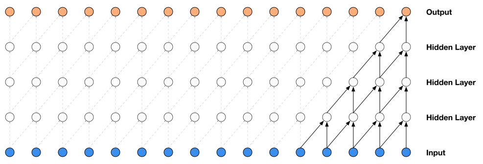
Figure 2: Visualization of a stack of causal convolutional layers.

图 2：一叠因果卷积层的示意图。

The main ingredient of WaveNet are causal convolutions. By using causal convolutions, we make sure the model cannot violate the ordering in which we model the data: the prediction $p\left(x_{t+1}\mid x_{1},...,x_{t}\right)$ emitted by the model at timestep $t$ cannot depend on any of the future timesteps $x_{t+1},x_{t+2},\dots,x_{T}$ as shown in Fig. 2. For images, the equivalent of a causal convolution is a masked convolution (van den Oord et al. 2016a) which can be implemented by constructing a mask tensor and doing an elementwise multiplication of this mask with the convolution kernel before applying it. For 1-D data such as audio one can more easily implement this by shifting the output of a normal convolution by a few timesteps.

WaveNet 的主要组成部分是因果卷积（causal convolution）。使用因果卷积可以确保模型不会违反数据建模的顺序：如图 2 所示，模型在时间步 $t$ 给出的预测 $p\left(x_{t+1}\mid x_{1},...,x_{t}\right)$ 不能依赖任何未来时间步 $x_{t+1},x_{t+2},\dots,x_{T}$。对图像来说，与因果卷积等价的是掩码卷积（masked convolution）（van den Oord et al. 2016a），实现方法是构造一个掩码张量，在应用卷积核之前把掩码与卷积核逐元素相乘。对于音频这样的一维数据，更简单的实现是把普通卷积的输出平移几个时间步。

At training time, the conditional predictions for all timesteps can be made in parallel because all timesteps of ground truth $\mathbf{x}$ are known. When generating with the model, the predictions are sequential: after each sample is predicted, it is fed back into the network to predict the next sample.

训练时，由于真实数据 $\mathbf{x}$ 的所有时间步都已知，所有时间步的条件预测可以并行完成。用模型生成时，预测是逐个进行的：每预测出一个采样点，就把它送回网络，用来预测下一个采样点。

Because models with causal convolutions do not have recurrent connections, they are typically faster to train than RNNs, especially when applied to very long sequences. One of the problems of causal convolutions is that they require many layers, or large filters to increase the receptive field. For example, in Fig. 2 the receptive field is only 5 (= #layers + filter length - 1). In this paper we use dilated convolutions to increase the receptive field by orders of magnitude, without greatly increasing computational cost.

因果卷积模型没有循环连接，所以训练通常比 RNN 快，在非常长的序列上尤其如此。因果卷积的一个问题是，需要很多层或很大的滤波器才能增大感受野。例如在图 2 中，感受野只有 5（= 层数 + 滤波器长度 - 1）。本文使用扩张卷积，把感受野扩大几个数量级，同时不会大幅增加计算成本。

A dilated convolution (also called à trous, or convolution with holes) is a convolution where the filter is applied over an area larger than its length by skipping input values with a certain step. It is equivalent to a convolution with a larger filter derived from the original filter by dilating it with zeros, but is significantly more efficient. A dilated convolution effectively allows the network to operate on a coarser scale than with a normal convolution. This is similar to pooling or strided convolutions, but here the output has the same size as the input. As a special case, dilated convolution with dilation $1$ yields the standard convolution. Fig. 3 depicts dilated causal convolutions for dilations $1$, $2$, $4$, and $8$. Dilated convolutions have previously been used in various contexts, e.g. signal processing (Holschneider et al. 1989; Dutilleux 1989), and image segmentation (Chen et al. 2015; Yu & Koltun 2016).

扩张卷积（dilated convolution，也称 à trous 卷积，或带孔卷积）是指滤波器以一定步长跳过输入值，从而作用在比自身长度更大的区域上。它等价于一个用零把原滤波器“撑大”后得到的更大滤波器所做的卷积，但效率高得多。与普通卷积相比，扩张卷积实际上让网络在更粗的尺度上运行。这与池化或带步长的卷积相似，只是这里输出与输入大小相同。作为特例，扩张系数为 $1$ 的扩张卷积就是标准卷积。图 3 画出了扩张系数分别为 $1$、$2$、$4$ 和 $8$ 的扩张因果卷积。扩张卷积此前已用于多种场景，例如信号处理（Holschneider et al. 1989; Dutilleux 1989）和图像分割（Chen et al. 2015; Yu & Koltun 2016）。

Figure 3: Visualization of a stack of dilated causal convolutional layers.

图 3：一叠扩张因果卷积层的示意图。

Stacked dilated convolutions enable networks to have very large receptive fields with just a few layers, while preserving the input resolution throughout the network as well as computational efficiency. In this paper, the dilation is doubled for every layer up to a limit and then repeated: e.g.

堆叠扩张卷积让网络只用很少几层就能获得非常大的感受野，同时在整个网络中保持输入分辨率和计算效率。本文中，扩张系数每层翻倍，到达上限后再重复，例如：

$$1,2,4,\dots,512,1,2,4,\dots,512,1,2,4,\dots,512.$$

The intuition behind this configuration is two-fold. First, exponentially increasing the dilation factor results in exponential receptive field growth with depth (Yu & Koltun 2016). For example each $1,2,4,\dots,512$ block has receptive field of size $1024$, and can be seen as a more efficient and discriminative (non-linear) counterpart of a $1\times 1024$ convolution. Second, stacking these blocks further increases the model capacity and the receptive field size.

这种配置背后的直觉有两点。第一，扩张系数指数增长，感受野随深度也呈指数增长（Yu & Koltun 2016）。例如，每个 $1,2,4,\dots,512$ 块的感受野大小为 $1024$，可以看作 $1\times 1024$ 卷积的一种更高效、更有判别力的（非线性）替代。第二，堆叠多个这样的块，进一步增加了模型容量和感受野大小。

2.2 Softmax distributions

2.2 Softmax 分布

One approach to modeling the conditional distributions $p\left(x_{t}\mid x_{1},\dots,x_{t-1}\right)$ over the individual audio samples would be to use a mixture model such as a mixture density network (Bishop 1994) or mixture of conditional Gaussian scale mixtures (MCGSM) (Theis & Bethge 2015). However, van den Oord et al. 2016a showed that a softmax distribution tends to work better, even when the data is implicitly continuous (as is the case for image pixel intensities or audio sample values). One of the reasons is that a categorical distribution is more flexible and can more easily model arbitrary distributions because it makes no assumptions about their shape.

对单个音频采样点上的条件分布 $p\left(x_{t}\mid x_{1},\dots,x_{t-1}\right)$ 建模，一种做法是使用混合模型，例如混合密度网络（mixture density network）（Bishop 1994）或条件高斯尺度混合的混合模型（MCGSM）（Theis & Bethge 2015）。不过，van den Oord et al. 2016a 表明，即使数据隐含是连续的（图像像素强度或音频采样值都是如此），softmax 分布的效果往往也更好。原因之一是类别分布更灵活，不对分布形状做任何假设，因此更容易建模任意分布。

Because raw audio is typically stored as a sequence of 16-bit integer values (one per timestep), a softmax layer would need to output 65,536 probabilities per timestep to model all possible values. To make this more tractable, we first apply a $\mu$-law companding transformation (ITU-T 1988) to the data, and then quantize it to 256 possible values:

原始音频通常存储为 16 位整数值的序列（每个时间步一个），softmax 层要建模所有可能的取值，每个时间步就需要输出 65,536 个概率。为了让问题更易处理，我们先对数据做 $\mu$ 律压扩变换（$\mu$-law companding transformation）（ITU-T 1988），再把它量化为 256 个可能的值：

$$f\left(x_{t}\right)=\operatorname{sign}(x_{t})\frac{\ln\left(1+\mu\left|x_{t}\right|\right)}{\ln\left(1+\mu\right)},$$

where $-1<x_{t}<1$ and $\mu=255$. This non-linear quantization produces a significantly better reconstruction than a simple linear quantization scheme. Especially for speech, we found that the reconstructed signal after quantization sounded very similar to the original.

其中 $-1<x_{t}<1$，$\mu=255$。这种非线性量化的重建效果明显好于简单的线性量化方案。特别是对语音，我们发现量化后重建的信号听起来与原始信号非常接近。

2.3 Gated activation units

2.3 门控激活单元

We use the same gated activation unit as used in the gated PixelCNN (van den Oord et al. 2016b):

我们使用与门控 PixelCNN（gated PixelCNN）（van den Oord et al. 2016b）相同的门控激活单元（gated activation unit）：

$$\mathbf{z}=\tanh\left(W_{f,k}\ast\mathbf{x}\right)\odot\sigma\left(W_{g,k}\ast\mathbf{x}\right), \tag{2}$$

where $\ast$ denotes a convolution operator, $\odot$ denotes an element-wise multiplication operator, $\sigma(\cdot)$ is a sigmoid function, $k$ is the layer index, $f$ and $g$ denote filter and gate, respectively, and $W$ is a learnable convolution filter. In our initial experiments, we observed that this non-linearity worked significantly better than the rectified linear activation function (Nair & Hinton 2010) for modeling audio signals.

其中 $\ast$ 表示卷积算子，$\odot$ 表示逐元素乘法算子，$\sigma(\cdot)$ 是 sigmoid 函数，$k$ 是层的编号，$f$ 和 $g$ 分别表示滤波器（filter）和门（gate），$W$ 是可学习的卷积滤波器。在最初的实验中我们观察到，建模音频信号时，这种非线性的效果明显好于线性整流激活函数（Nair & Hinton 2010）。

2.4 Residual and skip connections

2.4 残差连接和跳跃连接

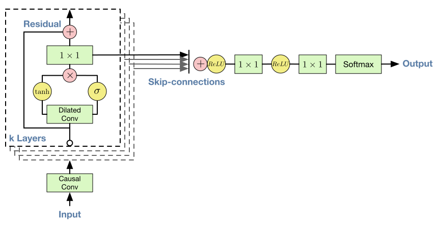
Figure 4: Overview of the residual block and the entire architecture.

图 4：残差块和整体架构概览。

Both residual (He et al. 2015) and parameterised skip connections are used throughout the network, to speed up convergence and enable training of much deeper models. In Fig. 4 we show a residual block of our model, which is stacked many times in the network.

整个网络都使用了残差连接（He et al. 2015）和带参数的跳跃连接，以加快收敛，并使更深的模型可以训练。图 4 画出了模型中的一个残差块，网络中堆叠了许多个这样的块。

2.5 Conditional WaveNets

2.5 条件 WaveNet

Given an additional input $\mathbf{h}$, WaveNets can model the conditional distribution $p\left(\mathbf{x}\mid\mathbf{h}\right)$ of the audio given this input. Eq. (1) now becomes

给定额外输入 $\mathbf{h}$，WaveNet 可以建模给定该输入时音频的条件分布 $p\left(\mathbf{x}\mid\mathbf{h}\right)$。式 (1) 变为

$$p\left(\mathbf{x}\mid\mathbf{h}\right)=\prod_{t=1}^{T}p\left(x_{t}\mid x_{1},\dots,x_{t-1},\mathbf{h}\right). \tag{3}$$

By conditioning the model on other input variables, we can guide WaveNet’s generation to produce audio with the required characteristics. For example, in a multi-speaker setting we can choose the speaker by feeding the speaker identity to the model as an extra input. Similarly, for TTS we need to feed information about the text as an extra input.

以其他输入变量为条件，可以引导 WaveNet 生成具有所需特征的音频。例如，在多说话人设置中，可以把说话人身份作为额外输入送入模型来选择说话人。同样，做 TTS 时需要把文本信息作为额外输入送入模型。

We condition the model on other inputs in two different ways: global conditioning and local conditioning. Global conditioning is characterised by a single latent representation $\mathbf{h}$ that influences the output distribution across all timesteps, e.g. a speaker embedding in a TTS model. The activation function from Eq. (2) now becomes:

我们用两种方式让模型以其他输入为条件：全局条件（global conditioning）和局部条件（local conditioning）。全局条件的特点是由单个潜在表示 $\mathbf{h}$ 影响所有时间步上的输出分布，例如 TTS 模型中的说话人嵌入。此时式 (2) 中的激活函数变为：

$$\mathbf{z}=\tanh\left(W_{f,k}\ast\mathbf{x}+V_{f,k}^{T}\mathbf{h}\right)\odot\sigma\left(W_{g,k}\ast\mathbf{x}+V_{g,k}^{T}\mathbf{h}\right).$$

where $V_{*,k}$ is a learnable linear projection, and the vector $V_{*,k}^{T}\mathbf{h}$ is broadcast over the time dimension.

其中 $V_{*,k}$ 是可学习的线性投影，向量 $V_{*,k}^{T}\mathbf{h}$ 沿时间维度广播。

For local conditioning we have a second timeseries $h_{t}$, possibly with a lower sampling frequency than the audio signal, e.g. linguistic features in a TTS model. We first transform this time series using a transposed convolutional network (learned upsampling) that maps it to a new time series $\mathbf{y}=f(\mathbf{h})$ with the same resolution as the audio signal, which is then used in the activation unit as follows:

局部条件则有第二个时间序列 $h_{t}$，它的采样频率可能低于音频信号，例如 TTS 模型中的语言学特征。我们先用一个转置卷积网络（学习得到的上采样）变换这个时间序列，把它映射为一个与音频信号分辨率相同的新时间序列 $\mathbf{y}=f(\mathbf{h})$，再按如下方式用于激活单元：

$$\mathbf{z}=\tanh\left(W_{f,k}\ast\mathbf{x}+V_{f,k}\ast\mathbf{y}\right)\odot\sigma\left(W_{g,k}\ast\mathbf{x}+V_{g,k}\ast\mathbf{y}\right),$$

where $V_{f,k}\ast\mathbf{y}$ is now a $1\times 1$ convolution. As an alternative to the transposed convolutional network, it is also possible to use $V_{f,k}\ast\mathbf{h}$ and repeat these values across time. We saw that this worked slightly worse in our experiments.

其中 $V_{f,k}\ast\mathbf{y}$ 现在是一个 $1\times 1$ 卷积。除了转置卷积网络，也可以用 $V_{f,k}\ast\mathbf{h}$，再把这些值沿时间重复。我们在实验中发现这种做法效果稍差。

2.6 Context stacks

2.6 上下文堆栈

We have already mentioned several different ways to increase the receptive field size of a WaveNet: increasing the number of dilation stages, using more layers, larger filters, greater dilation factors, or a combination thereof. A complementary approach is to use a separate, smaller context stack that processes a long part of the audio signal and locally conditions a larger WaveNet that processes only a smaller part of the audio signal (cropped at the end). One can use multiple context stacks with varying lengths and numbers of hidden units. Stacks with larger receptive fields have fewer units per layer. Context stacks can also have pooling layers to run at a lower frequency. This keeps the computational requirements at a reasonable level and is consistent with the intuition that less capacity is required to model temporal correlations at longer timescales.

前面已经提到几种增大 WaveNet 感受野的方法：增加扩张阶段的数量、使用更多层、更大的滤波器、更大的扩张系数，或者将它们组合起来。另一种互补的方法是使用一个单独的、较小的上下文堆栈（context stack），由它处理一长段音频信号，再对一个只处理较短音频片段（在末端截取）的较大 WaveNet 做局部条件。可以使用多个长度和隐藏单元数不同的上下文堆栈；感受野越大的堆栈，每层的单元越少。上下文堆栈也可以包含池化层，以较低的频率运行。这样能把计算需求控制在合理水平，也符合一个直觉：建模更长时间尺度上的时间相关性所需的容量更少。

3 Experiments

3 实验

To measure WaveNet’s audio modelling performance, we evaluate it on three different tasks: multi-speaker speech generation (not conditioned on text), TTS, and music audio modelling. We provide samples drawn from WaveNet for these experiments on the accompanying webpage: https://www.deepmind.com/blog/wavenet-generative-model-raw-audio/.

为了衡量 WaveNet 的音频建模性能，我们在三个不同任务上评估它：多说话人语音生成（不以文本为条件）、TTS 和音乐音频建模。这些实验中 WaveNet 生成的样本见配套网页：https://www.deepmind.com/blog/wavenet-generative-model-raw-audio/。

3.1 Multi-Speaker Speech Generation

3.1 多说话人语音生成

For the first experiment we looked at free-form speech generation (not conditioned on text). We used the English multi-speaker corpus from CSTR voice cloning toolkit (VCTK) (Yamagishi 2012) and conditioned WaveNet only on the speaker. The conditioning was applied by feeding the speaker ID to the model in the form of a one-hot vector. The dataset consisted of 44 hours of data from 109 different speakers.

第一个实验考察自由形式的语音生成（不以文本为条件）。我们使用 CSTR 声音克隆工具包（VCTK）（Yamagishi 2012）中的英语多说话人语料库，WaveNet 只以说话人为条件。条件信息以独热（one-hot）向量的形式把说话人 ID 送入模型。数据集包含 109 位不同说话人的 44 小时数据。

Because the model is not conditioned on text, it generates non-existent but human language-like words in a smooth way with realistic sounding intonations. This is similar to generative models of language or images, where samples look realistic at first glance, but are clearly unnatural upon closer inspection. The lack of long range coherence is partly due to the limited size of the model’s receptive field (about 300 milliseconds), which means it can only remember the last 2–3 phonemes it produced.

由于模型不以文本为条件，它会流畅地生成并不存在、但很像人类语言的词，语调听起来也很真实。这与语言或图像的生成模型类似：样本乍看很逼真，仔细检查就会发现明显不自然。缺乏长程连贯性，部分原因是模型的感受野有限（约 300 毫秒），这意味着它只能记住自己最近生成的 2–3 个音素。

A single WaveNet was able to model speech from any of the speakers by conditioning it on a one-hot encoding of a speaker. This confirms that it is powerful enough to capture the characteristics of all 109 speakers from the dataset in a single model. We observed that adding speakers resulted in better validation set performance compared to training solely on a single speaker. This suggests that WaveNet’s internal representation was shared among multiple speakers.

以说话人的独热编码为条件，单个 WaveNet 就能建模任一说话人的语音。这证实了它的能力足以在一个模型中捕捉数据集里全部 109 位说话人的特征。我们观察到，与只在单个说话人上训练相比，加入更多说话人能提高验证集上的表现。这表明 WaveNet 的内部表示在多个说话人之间是共享的。

Finally, we observed that the model also picked up on other characteristics in the audio apart from the voice itself. For instance, it also mimicked the acoustics and recording quality, as well as the breathing and mouth movements of the speakers.

最后，我们观察到模型还学到了嗓音本身以外的其他音频特征。例如，它也模仿了录音的声学环境和录音质量，以及说话人的呼吸声和嘴部动作声。

3.2 Text-To-Speech

3.2 文本转语音

For the second experiment we looked at TTS. We used the same single-speaker speech databases from which Google’s North American English and Mandarin Chinese TTS systems are built. The North American English dataset contains 24.6 hours of speech data, and the Mandarin Chinese dataset contains 34.8 hours; both were spoken by professional female speakers.

第二个实验考察 TTS。我们使用的单说话人语音数据库，与构建 Google 北美英语和普通话 TTS 系统所用的相同。北美英语数据集包含 24.6 小时语音，普通话数据集包含 34.8 小时，均由专业女性播音员录制。

WaveNets for the TTS task were locally conditioned on linguistic features which were derived from input texts. We also trained WaveNets conditioned on the logarithmic fundamental frequency ($\log F_{0}$) values in addition to the linguistic features. External models predicting $\log F_{0}$ values and phone durations from linguistic features were also trained for each language. The receptive field size of the WaveNets was 240 milliseconds. As example-based and model-based speech synthesis baselines, hidden Markov model (HMM)-driven unit selection concatenative (Gonzalvo et al. 2016) and long short-term memory recurrent neural network (LSTM-RNN)-based statistical parametric (Zen et al. 2016) speech synthesizers were built. Since the same datasets and linguistic features were used to train both the baselines and WaveNets, these speech synthesizers could be fairly compared.

用于 TTS 任务的 WaveNet 以从输入文本导出的语言学特征（linguistic features）为局部条件。我们还训练了在语言学特征之外再以对数基频（$\log F_{0}$）为条件的 WaveNet。每种语言还另外训练了根据语言学特征预测 $\log F_{0}$ 值和音素时长的外部模型。WaveNet 的感受野为 240 毫秒。作为基于样例和基于模型的语音合成基线，我们构建了基于隐马尔可夫模型（HMM）驱动的单元选择拼接式合成器（Gonzalvo et al. 2016），以及基于长短期记忆循环神经网络（LSTM-RNN）的统计参数式合成器（Zen et al. 2016）。基线和 WaveNet 使用相同的数据集和语言学特征训练，因此这些语音合成器可以公平比较。

To evaluate the performance of WaveNets for the TTS task, subjective paired comparison tests and mean opinion score (MOS) tests were conducted. In the paired comparison tests, after listening to each pair of samples, the subjects were asked to choose which they preferred, though they could choose “neutral” if they did not have any preference. In the MOS tests, after listening to each stimulus, the subjects were asked to rate the naturalness of the stimulus in a five-point Likert scale score (1: Bad, 2: Poor, 3: Fair, 4: Good, 5: Excellent). Please refer to Appendix B for details.

为了评估 WaveNet 在 TTS 任务上的表现，我们进行了主观成对比较测试和平均意见分（mean opinion score，MOS）测试。成对比较测试中，受试者每听完一对样本，要选出更喜欢的一个；如果没有偏好，也可以选“中立”。MOS 测试中，受试者每听完一个刺激，要用五点李克特量表（1：很差，2：较差，3：一般，4：好，5：很好）为其自然度打分。详见附录 B。

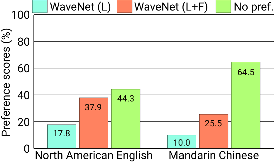
Fig. 5 shows a selection of the subjective paired comparison test results (see Appendix B for the complete table). It can be seen from the results that WaveNet outperformed the baseline statistical parametric and concatenative speech synthesizers in both languages. We found that WaveNet conditioned on linguistic features could synthesize speech samples with natural segmental quality but sometimes it had unnatural prosody by stressing wrong words in a sentence. This could be due to the long-term dependency of $F_{0}$ contours: the size of the receptive field of the WaveNet, 240 milliseconds, was not long enough to capture such long-term dependency. WaveNet conditioned on both linguistic features and $F_{0}$ values did not have this problem: the external $F_{0}$ prediction model runs at a lower frequency (200 Hz) so it can learn long-range dependencies that exist in $F_{0}$ contours.

图 5 给出了部分主观成对比较测试结果（完整表格见附录 B）。结果显示，在两种语言上，WaveNet 都优于统计参数式和拼接式基线合成器。我们发现，只以语言学特征为条件的 WaveNet 能合成音段质量自然的语音样本，但有时韵律不自然，会重读句子中不该重读的词。这可能是 $F_{0}$ 轮廓的长期依赖造成的：WaveNet 的感受野只有 240 毫秒，不足以捕捉这种长期依赖。同时以语言学特征和 $F_{0}$ 值为条件的 WaveNet 没有这个问题：外部 $F_{0}$ 预测模型以较低频率（200 Hz）运行，因此能学到 $F_{0}$ 轮廓中存在的长程依赖。

Figure 5: Subjective preference scores (%) of speech samples between (top) two baselines, (middle) two WaveNets, and (bottom) the best baseline and WaveNet. Note that LSTM and Concat correspond to LSTM-RNN-based statistical parametric and HMM-driven unit selection concatenative baseline synthesizers, and WaveNet (L) and WaveNet (L+F) correspond to the WaveNet conditioned on linguistic features only and that conditioned on both linguistic features and $\log F_{0}$ values.

图 5：语音样本的主观偏好得分（%），分别比较（上）两个基线、（中）两个 WaveNet、（下）最好的基线和 WaveNet。LSTM 和 Concat 分别指基于 LSTM-RNN 的统计参数式基线合成器和 HMM 驱动的单元选择拼接式基线合成器；WaveNet (L) 和 WaveNet (L+F) 分别指只以语言学特征为条件的 WaveNet，以及同时以语言学特征和 $\log F_{0}$ 值为条件的 WaveNet。

Table 1 show the MOS test results. It can be seen from the table that WaveNets achieved 5-scale MOSs in naturalness above 4.0, which were significantly better than those from the baseline systems. They were the highest ever reported MOS values with these training datasets and test sentences. The gap in the MOSs from the best synthetic speech to the natural ones decreased from 0.69 to 0.34 (51%) in US English and 0.42 to 0.13 (69%) in Mandarin Chinese.

表 1 给出了 MOS 测试结果。从表中可以看到，WaveNet 的五级自然度 MOS 超过 4.0，明显好于基线系统。这是在这些训练数据集和测试句子上报告过的最高 MOS 值。最好的合成语音与自然语音之间的 MOS 差距，在美国英语上从 0.69 缩小到 0.34（缩小 51%），在普通话上从 0.42 缩小到 0.13（缩小 69%）。

Speech samples	North American English	Mandarin Chinese
LSTM-RNN parametric	3.67 $\pm$ 0.098	3.79 $\pm$ 0.084
HMM-driven concatenative	3.86 $\pm$ 0.137	3.47 $\pm$ 0.108
WaveNet (L+F)	4.21 $\pm$ 0.081	4.08 $\pm$ 0.085
Natural (8-bit $\mu$-law)	4.46 $\pm$ 0.067	4.25 $\pm$ 0.082
Natural (16-bit linear PCM)	4.55 $\pm$ 0.075	4.21 $\pm$ 0.071

(Columns: subjective 5-scale MOS in naturalness.)

Table 1: Subjective 5-scale mean opinion scores of speech samples from LSTM-RNN-based statistical parametric, HMM-driven unit selection concatenative, and proposed WaveNet-based speech synthesizers, 8-bit $\mu$-law encoded natural speech, and 16-bit linear pulse-code modulation (PCM) natural speech. WaveNet improved the previous state of the art significantly, reducing the gap between natural speech and best previous model by more than 50%.

语音样本	北美英语	普通话
LSTM-RNN 参数式	3.67 $\pm$ 0.098	3.79 $\pm$ 0.084
HMM 驱动的拼接式	3.86 $\pm$ 0.137	3.47 $\pm$ 0.108
WaveNet (L+F)	4.21 $\pm$ 0.081	4.08 $\pm$ 0.085
自然语音（8 位 $\mu$ 律）	4.46 $\pm$ 0.067	4.25 $\pm$ 0.082
自然语音（16 位线性 PCM）	4.55 $\pm$ 0.075	4.21 $\pm$ 0.071

（各列为五级主观自然度 MOS。）

表 1：各类语音样本的五级主观平均意见分，包括基于 LSTM-RNN 的统计参数式合成器、HMM 驱动的单元选择拼接式合成器、本文提出的基于 WaveNet 的合成器，以及 8 位 $\mu$ 律编码的自然语音和 16 位线性脉冲编码调制（PCM）的自然语音。WaveNet 大幅改进了此前的最好水平，把自然语音与此前最好模型之间的差距缩小了 50% 以上。

3.3 Music

3.3 音乐

For out third set of experiments we trained WaveNets to model two music datasets:

第三组实验中，我们训练 WaveNet 建模两个音乐数据集：

• the MagnaTagATune dataset (Law & Von Ahn 2009), which consists of about 200 hours of music audio. Each 29-second clip is annotated with tags from a set of 188, which describe the genre, instrumentation, tempo, volume and mood of the music.
• the YouTube piano dataset, which consists of about 60 hours of solo piano music obtained from YouTube videos. Because it is constrained to a single instrument, it is considerably easier to model.

• MagnaTagATune 数据集（Law & Von Ahn 2009），包含约 200 小时的音乐音频。每个 29 秒的片段都标注了来自 188 个标签集合的标签，描述音乐的流派、配器、速度、音量和情绪。
• YouTube 钢琴数据集，包含约 60 小时从 YouTube 视频中获取的钢琴独奏音乐。由于只限一种乐器，它要容易建模得多。

Although it is difficult to quantitatively evaluate these models, a subjective evaluation is possible by listening to the samples they produce. We found that enlarging the receptive field was crucial to obtain samples that sounded musical. Even with a receptive field of several seconds, the models did not enforce long-range consistency which resulted in second-to-second variations in genre, instrumentation, volume and sound quality. Nevertheless, the samples were often harmonic and aesthetically pleasing, even when produced by unconditional models.

这些模型很难定量评估，但可以通过听它们生成的样本做主观评价。我们发现，扩大感受野对得到听起来像音乐的样本至关重要。即使感受野达到几秒，模型也无法保持长程一致性，流派、配器、音量和音质会每秒都在变化。尽管如此，样本往往和谐悦耳，即使是无条件模型生成的样本也是如此。

Of particular interest are conditional music models, which can generate music given a set of tags specifying e.g. genre or instruments. Similarly to conditional speech models, we insert biases that depend on a binary vector representation of the tags associated with each training clip. This makes it possible to control various aspects of the output of the model when sampling, by feeding in a binary vector that encodes the desired properties of the samples. We have trained such models on the MagnaTagATune dataset; although the tag data bundled with the dataset was relatively noisy and had many omissions, after cleaning it up by merging similar tags and removing those with too few associated clips, we found this approach to work reasonably well.

特别有意思的是条件音乐模型，它可以根据一组指定流派或乐器等的标签生成音乐。与条件语音模型类似，我们插入依赖于每个训练片段所带标签的二值向量表示的偏置项。这样在采样时，只要输入一个编码了所需样本属性的二值向量，就能控制模型输出的各个方面。我们在 MagnaTagATune 数据集上训练了这样的模型；数据集自带的标签相当嘈杂，缺漏也很多，但在合并相似标签、去掉关联片段过少的标签之后，我们发现这种方法效果还不错。

3.4 Speech Recognition

3.4 语音识别

Although WaveNet was designed as a generative model, it can straightforwardly be adapted to discriminative audio tasks such as speech recognition.

WaveNet 虽然是作为生成模型设计的，但可以直接改造用于语音识别等判别式音频任务。

Traditionally, speech recognition research has largely focused on using log mel-filterbank energies or mel-frequency cepstral coefficients (MFCCs), but has been moving to raw audio recently (Palaz et al. 2013; Tüske et al. 2014; Hoshen et al. 2015; Sainath et al. 2015). Recurrent neural networks such as LSTM-RNNs (Hochreiter & Schmidhuber 1997) have been a key component in these new speech classification pipelines, because they allow for building models with long range contexts. With WaveNets we have shown that layers of dilated convolutions allow the receptive field to grow longer in a much cheaper way than using LSTM units.

传统上，语音识别研究主要使用对数梅尔滤波器组能量或梅尔频率倒谱系数（MFCC），但近来开始转向原始音频（Palaz et al. 2013; Tüske et al. 2014; Hoshen et al. 2015; Sainath et al. 2015）。LSTM-RNN（Hochreiter & Schmidhuber 1997）等循环神经网络一直是这些新的语音分类流水线的关键组件，因为它们能构建具有长程上下文的模型。我们通过 WaveNet 表明，扩张卷积层能以比 LSTM 单元低得多的代价扩大感受野。

As a last experiment we looked at speech recognition with WaveNets on the TIMIT (Garofolo et al. 1993) dataset. For this task we added a mean-pooling layer after the dilated convolutions that aggregated the activations to coarser frames spanning 10 milliseconds (160$\times$ downsampling). The pooling layer was followed by a few non-causal convolutions. We trained WaveNet with two loss terms, one to predict the next sample and one to classify the frame, the model generalized better than with a single loss and achieved $18.8$ PER on the test set, which is to our knowledge the best score obtained from a model trained directly on raw audio on TIMIT.

最后一个实验中，我们在 TIMIT（Garofolo et al. 1993）数据集上考察用 WaveNet 做语音识别。为此我们在扩张卷积之后加了一个平均池化层，把激活聚合为每帧 10 毫秒的较粗的帧（160$\times$ 下采样）。池化层之后接几个非因果卷积。我们用两项损失训练 WaveNet，一项预测下一个采样点，一项对帧分类；与只用单一损失相比，模型泛化得更好，在测试集上达到 $18.8$ 的音素错误率（PER）。据我们所知，这是 TIMIT 上直接在原始音频上训练的模型取得的最好成绩。

4 Conclusion

4 结论

This paper has presented WaveNet, a deep generative model of audio data that operates directly at the waveform level. WaveNets are autoregressive and combine causal filters with dilated convolutions to allow their receptive fields to grow exponentially with depth, which is important to model the long-range temporal dependencies in audio signals. We have shown how WaveNets can be conditioned on other inputs in a global (e.g. speaker identity) or local way (e.g. linguistic features). When applied to TTS, WaveNets produced samples that outperform the current best TTS systems in subjective naturalness. Finally, WaveNets showed very promising results when applied to music audio modeling and speech recognition.

本文提出了 WaveNet，一个直接在波形层面运行的音频深度生成模型。WaveNet 是自回归的，它把因果滤波器与扩张卷积结合起来，让感受野随深度呈指数增长，这对建模音频信号中的长程时间依赖很重要。我们展示了如何以全局方式（例如说话人身份）或局部方式（例如语言学特征）让 WaveNet 以其他输入为条件。用于 TTS 时，WaveNet 生成的样本在主观自然度上超过了当前最好的 TTS 系统。最后，WaveNet 在音乐音频建模和语音识别上也展现了非常有希望的结果。

Acknowledgements

致谢

The authors would like to thank Lasse Espeholt, Jeffrey De Fauw and Grzegorz Swirszcz for their inputs, Adam Cain, Max Cant and Adrian Bolton for their help with artwork, Helen King, Steven Gaffney and Steve Crossan for helping to manage the project, Faith Mackinder for help with preparing the blogpost, James Besley for legal support and Demis Hassabis for managing the project and his inputs.

作者感谢 Lasse Espeholt、Jeffrey De Fauw 和 Grzegorz Swirszcz 提供的意见，感谢 Adam Cain、Max Cant 和 Adrian Bolton 在插图上的帮助，感谢 Helen King、Steven Gaffney 和 Steve Crossan 协助管理项目，感谢 Faith Mackinder 协助准备博客文章，感谢 James Besley 提供法律支持，感谢 Demis Hassabis 管理项目并提出意见。

References

参考文献

Agiomyrgiannakis (2015) Agiomyrgiannakis, Yannis. Vocaine the vocoder and applications is speech synthesis. In ICASSP, pp. 4230–4234, 2015.

Bishop (1994) Bishop, Christopher M. Mixture density networks. Technical Report NCRG/94/004, Neural Computing Research Group, Aston University, 1994.

Chen et al. (2015) Chen, Liang-Chieh, Papandreou, George, Kokkinos, Iasonas, Murphy, Kevin, and Yuille, Alan L. Semantic image segmentation with deep convolutional nets and fully connected CRFs. In ICLR, 2015. URL http://arxiv.org/abs/1412.7062.

Chiba & Kajiyama (1942) Chiba, Tsutomu and Kajiyama, Masato. The Vowel: Its Nature and Structure. Tokyo-Kaiseikan, 1942.

Dudley (1939) Dudley, Homer. Remaking speech. The Journal of the Acoustical Society of America, 11(2):169–177, 1939.

Dutilleux (1989) Dutilleux, Pierre. An implementation of the “algorithme à trous” to compute the wavelet transform. In Combes, Jean-Michel, Grossmann, Alexander, and Tchamitchian, Philippe (eds.), Wavelets: Time-Frequency Methods and Phase Space, pp. 298–304. Springer Berlin Heidelberg, 1989.

Fan et al. (2014) Fan, Yuchen, Qian, Yao, and Xie, Feng-Long, Soong Frank K. TTS synthesis with bidirectional LSTM based recurrent neural networks. In Interspeech, pp. 1964–1968, 2014.

Fant (1970) Fant, Gunnar. Acoustic Theory of Speech Production. Mouton De Gruyter, 1970.

Garofolo et al. (1993) Garofolo, John S., Lamel, Lori F., Fisher, William M., Fiscus, Jonathon G., and Pallett, David S. DARPA TIMIT acoustic-phonetic continuous speech corpus CD-ROM. NIST speech disc 1-1.1. NASA STI/Recon technical report, 93, 1993.

Gonzalvo et al. (2016) Gonzalvo, Xavi, Tazari, Siamak, Chan, Chun-an, Becker, Markus, Gutkin, Alexander, and Silen, Hanna. Recent advances in Google real-time HMM-driven unit selection synthesizer. In Interspeech, 2016. URL http://research.google.com/pubs/pub45564.html.

He et al. (2015) He, Kaiming, Zhang, Xiangyu, Ren, Shaoqing, and Sun, Jian. Deep residual learning for image recognition. CoRR, abs/1512.03385, 2015.

Hochreiter & Schmidhuber (1997) Hochreiter, S. and Schmidhuber, J. Long short-term memory. Neural Comput., 9(8):1735–1780, 1997.

Holschneider et al. (1989) Holschneider, Matthias, Kronland-Martinet, Richard, Morlet, Jean, and Tchamitchian, Philippe. A real-time algorithm for signal analysis with the help of the wavelet transform. In Combes, Jean-Michel, Grossmann, Alexander, and Tchamitchian, Philippe (eds.), Wavelets: Time-Frequency Methods and Phase Space, pp. 286–297. Springer Berlin Heidelberg, 1989.

Hoshen et al. (2015) Hoshen, Yedid, Weiss, Ron J., and Wilson, Kevin W. Speech acoustic modeling from raw multichannel waveforms. In ICASSP, pp. 4624–4628. IEEE, 2015.

Hunt & Black (1996) Hunt, Andrew J. and Black, Alan W. Unit selection in a concatenative speech synthesis system using a large speech database. In ICASSP, pp. 373–376, 1996.

Imai & Furuichi (1988) Imai, Satoshi and Furuichi, Chieko. Unbiased estimation of log spectrum. In EURASIP, pp. 203–206, 1988.

Itakura (1975) Itakura, Fumitada. Line spectrum representation of linear predictor coefficients of speech signals. The Journal of the Acoust. Society of America, 57(S1):S35–S35, 1975.

Itakura & Saito (1970) Itakura, Fumitada and Saito, Shuzo. A statistical method for estimation of speech spectral density and formant frequencies. Trans. IEICE, J53–A:35–42, 1970.

ITU-T (1988) ITU-T. Recommendation G. 711. Pulse Code Modulation (PCM) of voice frequencies, 1988.

Józefowicz et al. (2016) Józefowicz, Rafal, Vinyals, Oriol, Schuster, Mike, Shazeer, Noam, and Wu, Yonghui. Exploring the limits of language modeling. CoRR, abs/1602.02410, 2016. URL http://arxiv.org/abs/1602.02410.

Juang & Rabiner (1985) Juang, Biing-Hwang and Rabiner, Lawrence. Mixture autoregressive hidden Markov models for speech signals. IEEE Trans. Acoust. Speech Signal Process., pp. 1404–1413, 1985.

Kameoka et al. (2010) Kameoka, Hirokazu, Ohishi, Yasunori, Mochihashi, Daichi, and Le Roux, Jonathan. Speech analysis with multi-kernel linear prediction. In Spring Conference of ASJ, pp. 499–502, 2010. (in Japanese).

Karaali et al. (1997) Karaali, Orhan, Corrigan, Gerald, Gerson, Ira, and Massey, Noel. Text-to-speech conversion with neural networks: A recurrent TDNN approach. In Eurospeech, pp. 561–564, 1997.

Kawahara et al. (1999) Kawahara, Hideki, Masuda-Katsuse, Ikuyo, and de Cheveigné, Alain. Restructuring speech representations using a pitch-adaptive time-frequency smoothing and an instantaneous-frequency-based $f_{0}$ extraction: possible role of a repetitive structure in sounds. Speech Commn., 27:187–207, 1999.

Kawahara et al. (2001) Kawahara, Hideki, Estill, Jo, and Fujimura, Osamu. Aperiodicity extraction and control using mixed mode excitation and group delay manipulation for a high quality speech analysis, modification and synthesis system STRAIGHT. In MAVEBA, pp. 13–15, 2001.

Law & Von Ahn (2009) Law, Edith and Von Ahn, Luis. Input-agreement: a new mechanism for collecting data using human computation games. In Proceedings of the SIGCHI Conference on Human Factors in Computing Systems, pp. 1197–1206. ACM, 2009.

Maia et al. (2010) Maia, Ranniery, Zen, Heiga, and Gales, Mark J. F. Statistical parametric speech synthesis with joint estimation of acoustic and excitation model parameters. In ISCA SSW7, pp. 88–93, 2010.

Morise et al. (2016) Morise, Masanori, Yokomori, Fumiya, and Ozawa, Kenji. WORLD: A vocoder-based high-quality speech synthesis system for real-time applications. IEICE Trans. Inf. Syst., E99-D(7):1877–1884, 2016.

Moulines & Charpentier (1990) Moulines, Eric and Charpentier, Francis. Pitch synchronous waveform processing techniques for text-to-speech synthesis using diphones. Speech Commn., 9:453–467, 1990.

Muthukumar & Black (2014) Muthukumar, P. and Black, Alan W. A deep learning approach to data-driven parameterizations for statistical parametric speech synthesis. arXiv:1409.8558, 2014.

Nair & Hinton (2010) Nair, Vinod and Hinton, Geoffrey E. Rectified linear units improve restricted Boltzmann machines. In ICML, pp. 807–814, 2010.

Nakamura et al. (2014) Nakamura, Kazuhiro, Hashimoto, Kei, Nankaku, Yoshihiko, and Tokuda, Keiichi. Integration of spectral feature extraction and modeling for HMM-based speech synthesis. IEICE Trans. Inf. Syst., E97-D(6):1438–1448, 2014.

Palaz et al. (2013) Palaz, Dimitri, Collobert, Ronan, and Magimai-Doss, Mathew. Estimating phoneme class conditional probabilities from raw speech signal using convolutional neural networks. In Interspeech, pp. 1766–1770, 2013.

Peltonen et al. (2001) Peltonen, Sari, Gabbouj, Moncef, and Astola, Jaakko. Nonlinear filter design: methodologies and challenges. In IEEE ISPA, pp. 102–107, 2001.

Poritz (1982) Poritz, Alan B. Linear predictive hidden Markov models and the speech signal. In ICASSP, pp. 1291–1294, 1982.

Rabiner & Juang (1993) Rabiner, Lawrence and Juang, Biing-Hwang. Fundamentals of Speech Recognition. PrenticeHall, 1993.

Sagisaka et al. (1992) Sagisaka, Yoshinori, Kaiki, Nobuyoshi, Iwahashi, Naoto, and Mimura, Katsuhiko. ATR $\nu$-talk speech synthesis system. In ICSLP, pp. 483–486, 1992.

Sainath et al. (2015) Sainath, Tara N., Weiss, Ron J., Senior, Andrew, Wilson, Kevin W., and Vinyals, Oriol. Learning the speech front-end with raw waveform CLDNNs. In Interspeech, pp. 1–5, 2015.

Takaki & Yamagishi (2016) Takaki, Shinji and Yamagishi, Junichi. A deep auto-encoder based low-dimensional feature extraction from FFT spectral envelopes for statistical parametric speech synthesis. In ICASSP, pp. 5535–5539, 2016.

Takamichi et al. (2016) Takamichi, Shinnosuke, Toda, Tomoki, Black, Alan W., Neubig, Graham, Sakriani, Sakti, and Nakamura, Satoshi. Postfilters to modify the modulation spectrum for statistical parametric speech synthesis. IEEE/ACM Trans. Audio Speech Lang. Process., 24(4):755–767, 2016.

Theis & Bethge (2015) Theis, Lucas and Bethge, Matthias. Generative image modeling using spatial LSTMs. In NIPS, pp. 1927–1935, 2015.

Toda & Tokuda (2007) Toda, Tomoki and Tokuda, Keiichi. A speech parameter generation algorithm considering global variance for HMM-based speech synthesis. IEICE Trans. Inf. Syst., E90-D(5):816–824, 2007.

Toda & Tokuda (2008) Toda, Tomoki and Tokuda, Keiichi. Statistical approach to vocal tract transfer function estimation based on factor analyzed trajectory hmm. In ICASSP, pp. 3925–3928, 2008.

Tokuda (2011) Tokuda, Keiichi. Speech synthesis as a statistical machine learning problem. http://www.sp.nitech.ac.jp/~tokuda/tokuda_asru2011_for_pdf.pdf, 2011. Invited talk given at ASRU.

Tokuda & Zen (2015) Tokuda, Keiichi and Zen, Heiga. Directly modeling speech waveforms by neural networks for statistical parametric speech synthesis. In ICASSP, pp. 4215–4219, 2015.

Tokuda & Zen (2016) Tokuda, Keiichi and Zen, Heiga. Directly modeling voiced and unvoiced components in speech waveforms by neural networks. In ICASSP, pp. 5640–5644, 2016.

Tuerk & Robinson (1993) Tuerk, Christine and Robinson, Tony. Speech synthesis using artificial neural networks trained on cepstral coefficients. In Proc. Eurospeech, pp. 1713–1716, 1993.

Tüske et al. (2014) Tüske, Zoltán, Golik, Pavel, Schlüter, Ralf, and Ney, Hermann. Acoustic modeling with deep neural networks using raw time signal for LVCSR. In Interspeech, pp. 890–894, 2014.

Uria et al. (2015) Uria, Benigno, Murray, Iain, Renals, Steve, Valentini-Botinhao, Cassia, and Bridle, John. Modelling acoustic feature dependencies with artificial neural networks: Trajectory-RNADE. In ICASSP, pp. 4465–4469, 2015.

van den Oord et al. (2016a) van den Oord, Aäron, Kalchbrenner, Nal, and Kavukcuoglu, Koray. Pixel recurrent neural networks. arXiv preprint arXiv:1601.06759, 2016a.

van den Oord et al. (2016b) van den Oord, Aäron, Kalchbrenner, Nal, Vinyals, Oriol, Espeholt, Lasse, Graves, Alex, and Kavukcuoglu, Koray. Conditional image generation with PixelCNN decoders. CoRR, abs/1606.05328, 2016b. URL http://arxiv.org/abs/1606.05328.

Wu & Tokuda (2008) Wu, Yi-Jian and Tokuda, Keiichi. Minimum generation error training with direct log spectral distortion on LSPs for HMM-based speech synthesis. In Interspeech, pp. 577–580, 2008.

Yamagishi (2012) Yamagishi, Junichi. English multi-speaker corpus for CSTR voice cloning toolkit, 2012. URL http://homepages.inf.ed.ac.uk/jyamagis/page3/page58/page58.html.

Yoshimura (2002) Yoshimura, Takayoshi. Simultaneous modeling of phonetic and prosodic parameters, and characteristic conversion for HMM-based text-to-speech systems. PhD thesis, Nagoya Institute of Technology, 2002.

Yu & Koltun (2016) Yu, Fisher and Koltun, Vladlen. Multi-scale context aggregation by dilated convolutions. In ICLR, 2016. URL http://arxiv.org/abs/1511.07122.

Zen (2006) Zen, Heiga. An example of context-dependent label format for HMM-based speech synthesis in English, 2006. URL http://hts.sp.nitech.ac.jp/?Download.

Zen et al. (2007) Zen, Heiga, Tokuda, Keiichi, and Kitamura, Tadashi. Reformulating the HMM as a trajectory model by imposing explicit relationships between static and dynamic features. Comput. Speech Lang., 21(1):153–173, 2007.

Zen et al. (2009) Zen, Heiga, Tokuda, Keiichi, and Black, Alan W. Statistical parametric speech synthesis. Speech Commn., 51(11):1039–1064, 2009.

Zen et al. (2013) Zen, Heiga, Senior, Andrew, and Schuster, Mike. Statistical parametric speech synthesis using deep neural networks. In Proc. ICASSP, pp. 7962–7966, 2013.

Zen et al. (2016) Zen, Heiga, Agiomyrgiannakis, Yannis, Egberts, Niels, Henderson, Fergus, and Szczepaniak, Przemysław. Fast, compact, and high quality LSTM-RNN based statistical parametric speech synthesizers for mobile devices. In Interspeech, 2016. URL https://arxiv.org/abs/1606.06061.

Appendix A Text-to-Speech Background

附录 A 文本转语音背景

The goal of TTS synthesis is to render naturally sounding speech signals given a text to be synthesized. Human speech production process first translates a text (or concept) into movements of muscles associated with articulators and speech production-related organs. Then using air-flow from lung, vocal source excitation signals, which contain both periodic (by vocal cord vibration) and aperiodic (by turbulent noise) components, are generated. By filtering the vocal source excitation signals by time-varying vocal tract transfer functions controlled by the articulators, their frequency characteristics are modulated. Finally, the generated speech signals are emitted. The aim of TTS is to mimic this process by computers in some way.

TTS 合成的目标是根据待合成的文本生成听起来自然的语音信号。人类的语音产生过程，首先把文本（或概念）转化为与发音器官及语音产生相关器官的肌肉运动。然后，利用来自肺部的气流产生声源激励信号，其中包含周期成分（来自声带振动）和非周期成分（来自湍流噪声）。声源激励信号经过由发音器官控制、随时间变化的声道传递函数滤波，频率特性被调制。最后，生成的语音信号被发出。TTS 的目标是让计算机以某种方式模仿这一过程。

TTS can be viewed as a sequence-to-sequence mapping problem; from a sequence of discrete symbols (text) to a real-valued time series (speech signals). A typical TTS pipeline has two parts; 1) text analysis and 2) speech synthesis. The text analysis part typically includes a number of natural language processing (NLP) steps, such as sentence segmentation, word segmentation, text normalization, part-of-speech (POS) tagging, and grapheme-to-phoneme (G2P) conversion. It takes a word sequence as input and outputs a phoneme sequence with a variety of linguistic contexts. The speech synthesis part takes the context-dependent phoneme sequence as its input and outputs a synthesized speech waveform. This part typically includes prosody prediction and speech waveform generation.

TTS 可以看作一个序列到序列的映射问题：从离散符号序列（文本）映射到实值时间序列（语音信号）。典型的 TTS 流水线有两部分：1）文本分析，2）语音合成。文本分析部分通常包括一系列自然语言处理（NLP）步骤，例如分句、分词、文本规范化、词性（POS）标注和字素到音素（G2P）转换。它以词序列为输入，输出带有各种语言学上下文的音素序列。语音合成部分以上下文相关的音素序列为输入，输出合成的语音波形。这一部分通常包括韵律预测和语音波形生成。

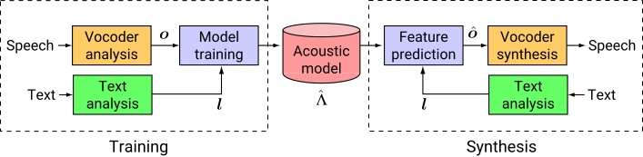
Figure 6: Outline of statistical parametric speech synthesis.

图 6：统计参数语音合成概览。

There are two main approaches to realize the speech synthesis part; non-parametric, example-based approach known as concatenative speech synthesis (Moulines & Charpentier 1990; Sagisaka et al. 1992; Hunt & Black 1996), and parametric, model-based approach known as statistical parametric speech synthesis (Yoshimura 2002; Zen et al. 2009). The concatenative approach builds up the utterance from units of recorded speech, whereas the statistical parametric approach uses a generative model to synthesize the speech. The statistical parametric approach first extracts a sequence of vocoder parameters (Dudley 1939) $\mathbf{o}=\{\mathbf{o}_{1},\dots,\mathbf{o}_{N}\}$ from speech signals $\mathbf{x}=\{x_{1},\dots,x_{T}\}$ and linguistic features $\mathbf{l}$ from the text $W$, where $N$ and $T$ correspond to the numbers of vocoder parameter vectors and speech signals. Typically a vocoder parameter vector $\mathbf{o}_{n}$ is extracted at every 5 milliseconds. It often includes cepstra (Imai & Furuichi 1988) or line spectral pairs (Itakura 1975), which represent vocal tract transfer function, and fundamental frequency ($F_{0}$) and aperiodicity (Kawahara et al. 2001), which represent characteristics of vocal source excitation signals. Then a set of generative models, such as hidden Markov models (HMMs) (Yoshimura 2002), feed-forward neural networks (Zen et al. 2013), and recurrent neural networks (Tuerk & Robinson 1993; Karaali et al. 1997; Fan et al. 2014), is trained from the extracted vocoder parameters and linguistic features as

实现语音合成部分有两种主要方法：一种是非参数的、基于样例的方法，称为拼接式语音合成（Moulines & Charpentier 1990; Sagisaka et al. 1992; Hunt & Black 1996）；另一种是参数的、基于模型的方法，称为统计参数语音合成（Yoshimura 2002; Zen et al. 2009）。拼接式方法用录制好的语音单元拼出整句话，统计参数方法则用生成模型合成语音。统计参数方法先从语音信号 $\mathbf{x}=\{x_{1},\dots,x_{T}\}$ 中提取声码器参数（Dudley 1939）序列 $\mathbf{o}=\{\mathbf{o}_{1},\dots,\mathbf{o}_{N}\}$，并从文本 $W$ 中提取语言学特征 $\mathbf{l}$，其中 $N$ 和 $T$ 分别是声码器参数向量和语音信号的数量。声码器参数向量 $\mathbf{o}_{n}$ 通常每 5 毫秒提取一次。它通常包括表示声道传递函数的倒谱（Imai & Furuichi 1988）或线谱对（Itakura 1975），以及表示声源激励信号特征的基频（$F_{0}$）和非周期性（Kawahara et al. 2001）。然后，用提取出的声码器参数和语言学特征训练一组生成模型，例如隐马尔可夫模型（HMM）（Yoshimura 2002）、前馈神经网络（Zen et al. 2013）和循环神经网络（Tuerk & Robinson 1993; Karaali et al. 1997; Fan et al. 2014）：

$$\hat{\Lambda}=\mathop{\mathrm{arg\,max}}_{\Lambda}p\left(\mathbf{o}\mid\mathbf{l},\Lambda\right), \tag{4}$$

where $\Lambda$ denotes the set of parameters of the generative model. At the synthesis stage, the most probable vocoder parameters are generated given linguistic features extracted from a text to be synthesized as

其中 $\Lambda$ 表示生成模型的参数集合。合成阶段，给定从待合成文本中提取的语言学特征，按下式生成最可能的声码器参数：

$$\hat{\mathbf{o}}=\mathop{\mathrm{arg\,max}}_{\mathbf{o}}p(\mathbf{o}\mid\mathbf{l},\hat{\Lambda}). \tag{5}$$

Then a speech waveform is reconstructed from $\hat{\mathbf{o}}$ using a vocoder. The statistical parametric approach offers various advantages over the concatenative one such as small footprint and flexibility to change its voice characteristics. However, its subjective naturalness is often significantly worse than that of the concatenative approach; synthesized speech often sounds muffled and has artifacts. Zen et al. 2009 reported three major factors that can degrade the subjective naturalness; quality of vocoders, accuracy of generative models, and effect of oversmoothing. The first factor causes the artifacts and the second and third factors lead to the muffleness in the synthesized speech. There have been a number of attempts to address these issues individually, such as developing high-quality vocoders (Kawahara et al. 1999; Agiomyrgiannakis 2015; Morise et al. 2016), improving the accuracy of generative models (Zen et al. 2007; Zen et al. 2013; Fan et al. 2014; Uria et al. 2015), and compensating the oversmoothing effect (Toda & Tokuda 2007; Takamichi et al. 2016). Zen et al. 2016 showed that state-of-the-art statistical parametric speech syntheziers matched state-of-the-art concatenative ones in some languages. However, its vocoded sound quality is still a major issue.

然后用声码器从 $\hat{\mathbf{o}}$ 重建语音波形。与拼接式方法相比，统计参数方法有不少优点，例如占用空间小、可以灵活改变音色特征。但它的主观自然度往往明显不如拼接式方法：合成语音常常听起来发闷，并带有杂音。Zen et al. 2009 报告了三个会降低主观自然度的主要因素：声码器的质量、生成模型的精度，以及过度平滑的影响。第一个因素导致杂音，第二和第三个因素导致合成语音发闷。已有许多工作分别处理这些问题，例如开发高质量声码器（Kawahara et al. 1999; Agiomyrgiannakis 2015; Morise et al. 2016）、提高生成模型的精度（Zen et al. 2007; Zen et al. 2013; Fan et al. 2014; Uria et al. 2015），以及补偿过度平滑效应（Toda & Tokuda 2007; Takamichi et al. 2016）。Zen et al. 2016 表明，在某些语言上，最先进的统计参数语音合成器已与最先进的拼接式合成器相当。但它经声码器处理后的音质仍是一个主要问题。

Extracting vocoder parameters can be viewed as estimation of a generative model parameters given speech signals (Itakura & Saito 1970; Imai & Furuichi 1988). For example, linear predictive analysis (Itakura & Saito 1970), which has been used in speech coding, assumes that the generative model of speech signals is a linear auto-regressive (AR) zero-mean Gaussian process;

提取声码器参数可以看作在给定语音信号时估计生成模型的参数（Itakura & Saito 1970; Imai & Furuichi 1988）。例如，语音编码中使用的线性预测分析（Itakura & Saito 1970）假设语音信号的生成模型是一个线性自回归（AR）零均值高斯过程：

$$\begin{aligned} x_{t}&=\sum_{p=1}^{P}a_{p}x_{t-p}+\epsilon_{t} \\ \epsilon_{t}&\sim\mathcal{N}(0,G^{2}) \end{aligned} \tag{6}$$

where $a_{p}$ is a $p$-th order linear predictive coefficient (LPC) and $G^{2}$ is a variance of modeling error. These parameters are estimated based on the maximum likelihood (ML) criterion. In this sense, the training part of the statistical parametric approach can be viewed as a two-step optimization and sub-optimal: extract vocoder parameters by fitting a generative model of speech signals then model trajectories of the extracted vocoder parameters by a separate generative model for time series (Tokuda 2011). There have been attempts to integrate these two steps into a single one (Toda & Tokuda 2008; Wu & Tokuda 2008; Maia et al. 2010; Nakamura et al. 2014; Muthukumar & Black 2014; Tokuda & Zen 2015; Tokuda & Zen 2016; Takaki & Yamagishi 2016). For example, Tokuda & Zen 2016 integrated non-stationary, nonzero-mean Gaussian process generative model of speech signals and LSTM-RNN-based sequence generative model to a single one and jointly optimized them by back-propagation. Although they showed that this model could approximate natural speech signals, its segmental naturalness was significantly worse than the non-integrated model due to over-generalization and over-estimation of noise components in speech signals.

其中 $a_{p}$ 是第 $p$ 阶线性预测系数（LPC），$G^{2}$ 是建模误差的方差。这些参数按最大似然（ML）准则估计。从这个意义上说，统计参数方法的训练部分可以看作一个两步的、次优的优化：先拟合语音信号的生成模型来提取声码器参数，再用另一个单独的时间序列生成模型对提取出的声码器参数轨迹建模（Tokuda 2011）。已有工作尝试把这两步合为一步（Toda & Tokuda 2008; Wu & Tokuda 2008; Maia et al. 2010; Nakamura et al. 2014; Muthukumar & Black 2014; Tokuda & Zen 2015; Tokuda & Zen 2016; Takaki & Yamagishi 2016）。例如，Tokuda & Zen 2016 把语音信号的非平稳、非零均值高斯过程生成模型与基于 LSTM-RNN 的序列生成模型整合为一个模型，并通过反向传播联合优化。他们表明这个模型能近似自然语音信号，但由于过度泛化和对语音信号中噪声成分的高估，其音段自然度明显不如未整合的模型。

The conventional generative models of raw audio signals have a number of assumptions which are inspired from the speech production, such as

传统的原始音频信号生成模型有一些受语音产生过程启发的假设，例如

• Use of fixed-length analysis window; They are typically based on a stationary stochastic process (Itakura & Saito 1970; Imai & Furuichi 1988; Poritz 1982; Juang & Rabiner 1985; Kameoka et al. 2010). To model time-varying speech signals by a stationary stochastic process, parameters of these generative models are estimated within a fixed-length, overlapping and shifting analysis window (typically its length is 20 to 30 milliseconds, and shift is 5 to 10 milliseconds). However, some phones such as stops are time-limited by less than 20 milliseconds (Rabiner & Juang 1993). Therefore, using such fixed-size analysis window has limitations.
• Linear filter; These generative models are typically realized as a linear time-invariant filter (Itakura & Saito 1970; Imai & Furuichi 1988; Poritz 1982; Juang & Rabiner 1985; Kameoka et al. 2010) within a windowed frame. However, the relationship between successive audio samples can be highly non-linear.
• Gaussian process assumption; The conventional generative models are based on Gaussian process (Itakura & Saito 1970; Imai & Furuichi 1988; Poritz 1982; Juang & Rabiner 1985; Kameoka et al. 2010; Tokuda & Zen 2015; Tokuda & Zen 2016). From the source-filter model of speech production (Chiba & Kajiyama 1942; Fant 1970) point of view, this is equivalent to assuming that a vocal source excitation signal is a sample from a Gaussian distribution (Itakura & Saito 1970; Imai & Furuichi 1988; Poritz 1982; Juang & Rabiner 1985; Tokuda & Zen 2015; Kameoka et al. 2010; Tokuda & Zen 2016). Together with the linear assumption above, it results in assuming that speech signals are normally distributed. However, distributions of real speech signals can be significantly different from Gaussian.

• 使用固定长度的分析窗口：这些模型通常基于平稳随机过程（Itakura & Saito 1970; Imai & Furuichi 1988; Poritz 1982; Juang & Rabiner 1985; Kameoka et al. 2010）。为了用平稳随机过程建模随时间变化的语音信号，这些生成模型的参数是在一个固定长度、相互重叠并不断平移的分析窗口内估计的（窗长通常为 20 到 30 毫秒，帧移为 5 到 10 毫秒）。然而，塞音等一些音素的持续时间不到 20 毫秒（Rabiner & Juang 1993）。因此，使用这种固定大小的分析窗口存在局限。
• 线性滤波器：这些生成模型通常在加窗的帧内实现为线性时不变滤波器（Itakura & Saito 1970; Imai & Furuichi 1988; Poritz 1982; Juang & Rabiner 1985; Kameoka et al. 2010）。然而，相邻音频采样点之间的关系可能是高度非线性的。
• 高斯过程假设：传统生成模型基于高斯过程（Itakura & Saito 1970; Imai & Furuichi 1988; Poritz 1982; Juang & Rabiner 1985; Kameoka et al. 2010; Tokuda & Zen 2015; Tokuda & Zen 2016）。从语音产生的源-滤波器模型（Chiba & Kajiyama 1942; Fant 1970）来看，这等价于假设声源激励信号是来自高斯分布的样本（Itakura & Saito 1970; Imai & Furuichi 1988; Poritz 1982; Juang & Rabiner 1985; Tokuda & Zen 2015; Kameoka et al. 2010; Tokuda & Zen 2016）。再加上前面的线性假设，就相当于假设语音信号服从正态分布。然而，真实语音信号的分布可能与高斯分布有显著差异。

Although these assumptions are convenient, samples from these generative models tend to be noisy and lose important details to make these audio signals sounding natural.

这些假设虽然方便，但这些生成模型产生的样本往往带有噪声，并丢失了让音频听起来自然的重要细节。

WaveNet, which was described in Section 2, has none of the above-mentioned assumptions. It incorporates almost no prior knowledge about audio signals, except the choice of the receptive field and $\mu$-law encoding of the signal. It can also be viewed as a non-linear causal filter for quantized signals. Although such non-linear filter can represent complicated signals while preserving the details, designing such filters is usually difficult (Peltonen et al. 2001). WaveNets give a way to train them from data.

第 2 节介绍的 WaveNet 不含上述任何假设。除了感受野的选择和信号的 $\mu$ 律编码，它几乎不引入关于音频信号的先验知识。它也可以看作一个针对量化信号的非线性因果滤波器。这种非线性滤波器能够在保留细节的同时表示复杂信号，但通常很难设计（Peltonen et al. 2001）。WaveNet 提供了一种从数据中训练这类滤波器的方法。

Appendix B Details of TTS Experiment

附录 B TTS 实验细节

The HMM-driven unit selection and WaveNet TTS systems were built from speech at 16 kHz sampling. Although LSTM-RNNs were trained from speech at 22.05 kHz sampling, speech at 16 kHz sampling was synthesized at runtime using a resampling functionality in the Vocaine vocoder (Agiomyrgiannakis 2015). Both the LSTM-RNN-based statistical parametric and HMM-driven unit selection speech synthesizers were built from the speech datasets in the 16-bit linear PCM, whereas the WaveNet-based ones were trained from the same speech datasets in the 8-bit $\mu$-law encoding.

HMM 驱动的单元选择 TTS 系统和 WaveNet TTS 系统都由 16 kHz 采样的语音构建。LSTM-RNN 是在 22.05 kHz 采样的语音上训练的，但运行时借助 Vocaine 声码器（Agiomyrgiannakis 2015）的重采样功能合成 16 kHz 采样的语音。基于 LSTM-RNN 的统计参数式合成器和 HMM 驱动的单元选择合成器都用 16 位线性 PCM 格式的语音数据集构建，而基于 WaveNet 的合成器用的是同一批语音数据集的 8 位 $\mu$ 律编码版本。

The linguistic features include phone, syllable, word, phrase, and utterance-level features (Zen 2006) (e.g. phone identities, syllable stress, the number of syllables in a word, and position of the current syllable in a phrase) with additional frame position and phone duration features (Zen et al. 2013). These features were derived and associated with speech every 5 milliseconds by phone-level forced alignment at the training stage. We used LSTM-RNN-based phone duration and autoregressive CNN-based $\log F_{0}$ prediction models. They were trained so as to minimize the mean squared errors (MSE). It is important to note that no post-processing was applied to the audio signals generated from the WaveNets.

语言学特征包括音素、音节、词、短语和语句层面的特征（Zen 2006）（例如音素身份、音节重音、词中的音节数、当前音节在短语中的位置），另加帧位置和音素时长特征（Zen et al. 2013）。训练阶段，这些特征通过音素级强制对齐导出，并每 5 毫秒与语音对应一次。我们使用基于 LSTM-RNN 的音素时长预测模型和基于自回归 CNN 的 $\log F_{0}$ 预测模型，二者都以最小化均方误差（MSE）为目标训练。需要指出的是，WaveNet 生成的音频信号没有经过任何后处理。

The subjective listening tests were blind and crowdsourced. 100 sentences not included in the training data were used for evaluation. Each subject could evaluate up to 8 and 63 stimuli for North American English and Mandarin Chinese, respectively. Test stimuli were randomly chosen and presented for each subject. In the paired comparison test, each pair of speech samples was the same text synthesized by the different models. In the MOS test, each stimulus was presented to subjects in isolation. Each pair was evaluated by eight subjects in the paired comparison test, and each stimulus was evaluated by eight subjects in the MOS test. The subjects were paid and native speakers performing the task. Those ratings (about 40%) where headphones were not used were excluded when computing the preference and mean opinion scores. Table 2 shows the full details of the paired comparison test shown in Fig. 5.

主观听力测试是盲测，通过众包进行。评估使用 100 个不在训练数据中的句子。北美英语和普通话测试中，每位受试者最多分别可评估 8 个和 63 个刺激。测试刺激随机选取并呈现给每位受试者。成对比较测试中，每对语音样本是由不同模型合成的同一段文本。MOS 测试中，每个刺激单独呈现给受试者。成对比较测试中每对样本由 8 位受试者评估，MOS 测试中每个刺激也由 8 位受试者评估。受试者是有报酬的母语者。计算偏好得分和平均意见分时，排除了没有使用耳机的评分（约占 40%）。表 2 给出了图 5 所示成对比较测试的完整结果。

Language	LSTM	Concat	WaveNet (L)	WaveNet (L+F)	No preference	$p$ value
North American English	23.3	63.6			13.1	$\ll 10^{-9}$
North American English	18.7		69.3		12.0	$\ll 10^{-9}$
North American English	7.6			82.0	10.4	$\ll 10^{-9}$
North American English		32.4	41.2		26.4	$0.003$
North American English		20.1		49.3	30.6	$\ll 10^{-9}$
North American English			17.8	37.9	44.3	$\ll 10^{-9}$
Mandarin Chinese	50.6	15.6			33.8	$\ll 10^{-9}$
Mandarin Chinese	25.0		23.3		51.8	0.476
Mandarin Chinese	12.5			29.3	58.2	$\ll 10^{-9}$
Mandarin Chinese		17.6	43.1		39.3	$\ll 10^{-9}$
Mandarin Chinese		7.6		55.9	36.5	$\ll 10^{-9}$
Mandarin Chinese			10.0	25.5	64.5	$\ll 10^{-9}$

(Values: subjective preference (%) in naturalness.)

Table 2: Subjective preference scores of speech samples between LSTM-RNN-based statistical parametric (LSTM), HMM-driven unit selection concatenative (Concat), and proposed WaveNet-based speech synthesizers. Each row of the table denotes scores of a paired comparison test between two synthesizers. Scores of the synthesizers which were significantly better than their competing ones at $p<0.01$ level were shown in the bold type. Note that WaveNet (L) and WaveNet (L+F) correspond to WaveNet conditioned on linguistic features only and that conditioned on both linguistic features and $F_{0}$ values.

语言	LSTM	Concat	WaveNet (L)	WaveNet (L+F)	无偏好	$p$ 值
北美英语	23.3	63.6			13.1	$\ll 10^{-9}$
北美英语	18.7		69.3		12.0	$\ll 10^{-9}$
北美英语	7.6			82.0	10.4	$\ll 10^{-9}$
北美英语		32.4	41.2		26.4	$0.003$
北美英语		20.1		49.3	30.6	$\ll 10^{-9}$
北美英语			17.8	37.9	44.3	$\ll 10^{-9}$
普通话	50.6	15.6			33.8	$\ll 10^{-9}$
普通话	25.0		23.3		51.8	0.476
普通话	12.5			29.3	58.2	$\ll 10^{-9}$
普通话		17.6	43.1		39.3	$\ll 10^{-9}$
普通话		7.6		55.9	36.5	$\ll 10^{-9}$
普通话			10.0	25.5	64.5	$\ll 10^{-9}$

（表中数值为自然度的主观偏好百分比。）

表 2：基于 LSTM-RNN 的统计参数式合成器（LSTM）、HMM 驱动的单元选择拼接式合成器（Concat）与本文提出的基于 WaveNet 的合成器之间，语音样本的主观偏好得分。表中每一行是两个合成器之间一次成对比较测试的得分。在 $p<0.01$ 水平上显著优于对手的合成器得分用粗体标出。WaveNet (L) 和 WaveNet (L+F) 分别指只以语言学特征为条件的 WaveNet，以及同时以语言学特征和 $F_{0}$ 值为条件的 WaveNet。