WaveGlow: A Flow-based Generative Network for Speech Synthesis

WaveGlow：用于语音合成的基于流的生成网络

Ryan Prenger    Rafael Valle    Bryan Catanzaro

Abstract

摘要

In this paper we propose WaveGlow: a flow-based network capable of generating high quality speech from mel-spectrograms. WaveGlow combines insights from Glow [1] and WaveNet [2] in order to provide fast, efficient and high-quality audio synthesis, without the need for auto-regression. WaveGlow is implemented using only a single network, trained using only a single cost function: maximizing the likelihood of the training data, which makes the training procedure simple and stable. Our PyTorch implementation produces audio samples at a rate of more than 500 kHz on an NVIDIA V100 GPU. Mean Opinion Scores show that it delivers audio quality as good as the best publicly available WaveNet implementation. All code will be made publicly available online [3].

本文提出 WaveGlow：一个基于流的网络，能够从梅尔谱（mel-spectrogram）生成高质量语音。WaveGlow 结合了 Glow[1] 与 WaveNet[2] 的思路，从而在无需自回归的前提下，提供快速、高效且高质量的音频合成。WaveGlow 只用单个网络实现，也只用单一代价函数训练：最大化训练数据的似然，因此训练过程简单且稳定。我们的 PyTorch 实现在一块 NVIDIA V100 GPU 上能以超过 500 kHz 的速率生成音频采样。平均意见分（Mean Opinion Score，MOS）显示，它给出的音质与当时公开可得的最好 WaveNet 实现相当。全部代码将在网上公开[3]。

1 Introduction

1 引言

Index Terms:

As voice interactions with machines become increasingly useful, efficiently synthesizing high quality speech becomes increasingly important. Small changes in voice quality or latency have large impacts on customer experience and customer preferences. However, high quality, real-time speech synthesis remains a challenging task. Speech synthesis requires generating very high dimensional samples with strong long term dependencies. Additionally, humans are sensitive to statistical imperfections in audio samples. Beyond the quality challenges, real-time speech synthesis has challenging speed and computation constraints. Perceived speech quality drops significantly when the audio sampling rate is less than 16kHz, and higher sampling rates generate even higher quality speech. Furthermore, many applications require synthesis rates much faster than 16kHz. For example, when synthesizing speech on remote servers, strict interactivity requirements mean the utterances must be synthesized quickly at sample rates far exceeding real-time requirements.

索引词：

随着人与机器的语音交互变得越来越有用，高效地合成高质量语音也变得越来越重要。音质或延迟上的小变化，就会对用户体验和偏好产生很大影响。然而，高质量的实时语音合成仍然困难。语音合成需要生成维度很高、又带有很强长期依赖的采样；此外，人对音频里的统计瑕疵相当敏感。除了音质本身，实时语音合成还面临速度和计算上的约束。音频采样率低于 16 kHz 时，感知音质会明显下降，更高的采样率则能生成更高质量的语音。而且许多应用要求合成速率远高于 16 kHz。例如，在远程服务器上合成语音时，严格的交互性要求意味着话语必须以远超实时的采样率尽快合成出来。

Currently, state of the art speech synthesis models are based on parametric neural networks. Text-to-speech synthesis is typically done in two steps. The first step transforms the text into time-aligned features, such as a mel-spectrogram [4, 5], or $\mathrm{F0}$ frequencies and other linguistic features [2, 6]. A second model transforms these time-aligned features into audio samples. This second model, sometimes referred to as a vocoder, is computationally challenging and affects quality as well. We focus on this second model in this work. Most of the neural network based models for speech synthesis are auto-regressive, meaning that they condition future audio samples on previous samples in order to model long term dependencies. These approaches are relatively simple to implement and train. However, they are inherently serial, and hence can’t fully utilize parallel processors like GPUs or TPUs. Models in this group often have difficulty synthesizing audio faster than 16kHz without sacrificing quality.

目前，最先进的语音合成模型基于参数化神经网络。文本转语音通常分两步。第一步把文本变成时间对齐的特征，例如梅尔谱[4, 5]，或基频 $\mathrm{F0}$ 与其他语言学特征[2, 6]。第二个模型再把这些时间对齐的特征变成音频采样。这第二个模型有时被称为声码器（vocoder），计算量大，也会影响音质。本文关注的就是这第二个模型。大多数基于神经网络的语音合成模型是自回归的，也就是用已经生成的采样来条件化未来的采样，以便刻画长期依赖。这类方法实现和训练都相对简单。但它们本质上是串行的，因而无法充分利用 GPU 或 TPU 这类并行处理器。这一组里的模型，往往很难在不牺牲音质的前提下，把合成速度做到超过 16 kHz。

At this time we know of three neural network based models that can synthesize speech without auto-regression: Parallel WaveNet [2], Clarinet [7], and MCNN for spectrogram inversion [8]. These techniques can synthesize audio at more than 500kHz on a GPU. However, these models are more difficult to train and implement than the auto-regressive models. All three require compound loss functions to improve audio quality or problems with mode collapse [9, 7, 8]. In addition, Parallel WaveNet and Clarinet require two networks, a student network and teacher network. The student networks underlying both Parallel WaveNet and Clarinet use Inverse Auto-regressive Flows (IAF) [10]. Though the IAF networks can be run in parallel at inference time, the auto-regressive nature of the flow itself makes calculation of the IAF inefficient. To overcome this, these works use a teacher network to train a student network on a approximation to the true likelihood. These approaches are hard to reproduce and deploy because of the difficulty of training these models successfully to convergence.

据我们所知，当时已有三种基于神经网络、且不必自回归就能合成语音的模型：Parallel WaveNet[2]、Clarinet[7]，以及用于谱图反演的 MCNN[8]。这些技术可以在 GPU 上以超过 500 kHz 的速率合成音频。不过，它们比自回归模型更难训练和实现。三者都需要复合损失函数，以改善音质或应对模式崩塌（mode collapse）问题[9, 7, 8]。此外，Parallel WaveNet 与 Clarinet 需要两套网络：学生网络和教师网络。两者底层的学生网络都使用逆自回归流（Inverse Auto-regressive Flows，IAF）[10]。尽管 IAF 网络在推断时可以并行运行，流本身的自回归性质却使 IAF 的似然计算没有效率。为克服这一点，这些工作用教师网络去训练学生网络，优化的是对真实似然的一种近似。由于很难把这些模型成功训练到收敛，它们不易复现，也不易部署。

In this work, we show that an auto-regressive flow is unnecessary for synthesizing speech. Our contribution is a flow-based network capable of generating high quality speech from mel-spectrograms. We refer to this network as WaveGlow, as it combines ideas from Glow [1] and WaveNet [2]. WaveGlow is simple to implement and train, using only a single network, trained using only the likelihood loss function. Despite the simplicity of the model, our PyTorch implementation synthesizes speech at more than 500kHz on an NVIDIA V100 GPU: more than 25 times faster than real time. Mean Opinion Scores show that it delivers audio quality as good as the best publicly available WaveNet implementation trained on the same dataset.

在本工作中，我们表明合成语音并不需要自回归流。我们的贡献是一个基于流的网络，能够从梅尔谱生成高质量语音。我们把它称为 WaveGlow，因为它结合了 Glow[1] 与 WaveNet[2] 的想法。WaveGlow 实现和训练都很简单：只用单个网络，也只用似然损失函数来训练。尽管模型简单，我们的 PyTorch 实现仍能在一块 NVIDIA V100 GPU 上以超过 500 kHz 的速率合成语音，也就是比实时快 25 倍以上。平均意见分显示，它给出的音质与在同一数据集上训练的、当时公开可得的最好 WaveNet 实现相当。

2 WaveGlow

WaveGlow is a generative model that generates audio by sampling from a distribution. To use a neural network as a generative model, we take samples from a simple distribution, in our case, a zero mean spherical Gaussian with the same number of dimensions as our desired output, and put those samples through a series of layers that transforms the simple distribution to one which has the desired distribution. In this case, we model the distribution of audio samples conditioned on a mel-spectrogram.

WaveGlow 是一个生成模型，通过从某个分布中采样来生成音频。要把神经网络当作生成模型来用，我们先从一个简单分布中取样——在我们这里，是与期望输出维数相同的零均值球形高斯——再让这些样本经过一串层，把简单分布变换成具有目标分布的分布。在这里，我们建模的是以梅尔谱为条件的音频采样分布。

$$\displaystyle\boldsymbol{z}\sim\mathcal{N}(\boldsymbol{z};0,\boldsymbol{I}) \\ \displaystyle\boldsymbol{x}=\boldsymbol{f}_{0}\circ\boldsymbol{f}_{1}\circ\ldots\boldsymbol{f}_{k}(\boldsymbol{z}) \tag{1}$$

We would like to train this model by directly minimizing the negative log-likelihood of the data. If we use an arbitrary neural network this is intractable. Flow-based networks [11, 12, 1] solve this problem by ensuring the neural network mapping is invertible. By restricting each layer to be bijective, the likelihood can be calculated directly using a change of variables:

我们希望通过直接最小化数据的负对数似然来训练这个模型。如果使用任意神经网络，这一点是不可行的。基于流的网络[11, 12, 1]通过保证神经网络映射可逆来解决这个问题。把每一层都限制为双射之后，似然就可以用变量替换直接计算：

$$\displaystyle\log{p_{\theta}(\boldsymbol{x})}=\log{p_{\theta}(\boldsymbol{z})}+\sum_{i=1}^{k}\log|\det(\boldsymbol{J}(\boldsymbol{f}_{i}^{-1}(\boldsymbol{x})))| \\ \displaystyle\boldsymbol{z}=\boldsymbol{f}_{k}^{-1}\circ\boldsymbol{f}_{k-1}^{-1}\circ\ldots\boldsymbol{f}_{0}^{-1}(\boldsymbol{x}) \tag{3}$$

In our case, the first term is the log-likelihood of the spherical Gaussian. This term penalizes the $l_{2}$ norm of the transformed sample. The second term arises from the change of variables, and the $\boldsymbol{J}$ is the Jacobian. The log-determinant of the Jacobian rewards any layer for increasing the volume of the space during the forward pass. This term also keeps a layer from just multiplying the $\boldsymbol{x}$ terms by zero to optimize the $l_{2}$ norm. The sequence of transformations is also referred to as a normalizing flow [13].

在我们这里，第一项是球形高斯的对数似然。这一项惩罚变换后样本的 $l_{2}$ 范数。第二项来自变量替换，其中 $\boldsymbol{J}$ 是雅可比矩阵。雅可比行列式的对数会奖励任何在前向传播中增大空间体积的层。这一项也阻止某一层只是把 $\boldsymbol{x}$ 各项乘以零来优化 $l_{2}$ 范数。这一串变换也被称为规范化流（normalizing flow）[13]。

Our model is most similar to the recent Glow work [1], and is depicted in figure 1. For the forward pass through the network, we take groups of 8 audio samples as vectors, which we call the ”squeeze” operation, as in [1]. We then process these vectors through several ”steps of flow”. A step of flow here consists of an invertible $1\times 1$ convolution followed by an affine coupling layer, described below.

我们的模型与近期的 Glow 工作[1]最为相近，结构如图 1 所示。网络的前向传播中，我们把每 8 个音频采样编成一组向量，这一步按[1]称为“挤压”（squeeze）操作。随后让这些向量经过若干“流步骤”（steps of flow）。这里的一个流步骤由一个可逆 $1\times 1$ 卷积，再加上下面描述的仿射耦合层组成。

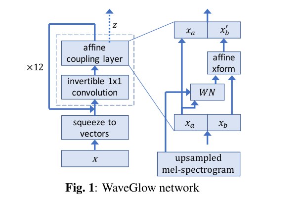
Figure 1: WaveGlow network

图 1：WaveGlow 网络

2.1 Affine Coupling Layer

2.1 仿射耦合层

Invertible neural networks are typically constructed using coupling layers [11, 12, 1]. In our case, we use an affine coupling layer [12]. Half of the channels serve as inputs, which then produce multiplicative and additive terms that are used to scale and translate the remaining channels:

可逆神经网络通常用耦合层来构造[11, 12, 1]。我们这里使用仿射耦合层[12]。一半通道作为输入，产生乘性项和加性项，再用来缩放和平移剩余通道：

$$\displaystyle\boldsymbol{x}_{a},\boldsymbol{x}_{b}=split(\boldsymbol{x}) \\ \displaystyle(\log\boldsymbol{s},\boldsymbol{t})=WN(\boldsymbol{x}_{a},\mathit{mel\textnormal{-}spectrogram}) \\ \displaystyle\boldsymbol{x}_{b}\prime=\boldsymbol{s}\odot\boldsymbol{x}_{b}+\boldsymbol{t} \\ \displaystyle\boldsymbol{f}_{coupling}^{-1}(\boldsymbol{x})=concat(\boldsymbol{x}_{a},\boldsymbol{x}_{b}\prime) \tag{5}$$

Here $WN()$ can be any transformation. The coupling layer preserves invertibility for the overall network, even though $WN()$ does not need to be invertible. This follows because the channels used as the inputs to $WN()$, in this case $\boldsymbol{x}_{a}$, are passed through unchanged to the output of the layer. Accordingly, when inverting the network, we can compute $\boldsymbol{s}$ and $\boldsymbol{t}$ from the output $\boldsymbol{x}_{a}$, and then invert $\boldsymbol{x}_{b}\prime$ to compute $\boldsymbol{x}_{b}$, by simply recomputing $WN(\boldsymbol{x}_{a},\mathit{mel\textnormal{-}spectrogram})$. In our case, $WN()$ uses layers of dilated convolutions with gated-$\tanh$ nonlinearities, as well as residual connections and skip connections. This $WN$ architecture is similar to WaveNet [2] and Parallel WaveNet [9], but our convolutions have 3 taps and are not causal. The affine coupling layer is also where we include the mel-spectrogram in order to condition the generated result on the input. The upsampled mel-spectrograms are added before the gated-$\tanh$ nonlinearites of each layer as in WaveNet [2].

这里的 $WN()$ 可以是任意变换。即使 $WN()$ 本身不必可逆，耦合层仍能保证整个网络可逆。原因在于：作为 $WN()$ 输入的那些通道，在我们这里是 $\boldsymbol{x}_{a}$，会原样传到该层输出。于是在反演网络时，我们可以从输出中的 $\boldsymbol{x}_{a}$ 算出 $\boldsymbol{s}$ 和 $\boldsymbol{t}$，再反演 $\boldsymbol{x}_{b}\prime$ 得到 $\boldsymbol{x}_{b}$，只需重新计算 $WN(\boldsymbol{x}_{a},\mathit{mel\textnormal{-}spectrogram})$。在我们这里，$WN()$ 使用带门控 $\tanh$ 非线性的膨胀卷积层，并带有残差连接和跳跃连接。这一 $WN$ 结构类似 WaveNet[2] 与 Parallel WaveNet[9]，但我们的卷积是 3 抽头的，并且不是因果的。仿射耦合层也是我们把梅尔谱引入、从而让生成结果条件于输入的地方。上采样后的梅尔谱会像 WaveNet[2] 那样，在每一层的门控 $\tanh$ 非线性之前被加入。

With an affine coupling layer, only the $\boldsymbol{s}$ term changes the volume of the mapping and adds a change of variables term to the loss. This term also serves to penalize the model for non-invertible affine mappings.

在仿射耦合层里，只有 $\boldsymbol{s}$ 项会改变映射的体积，并给损失增加一项变量替换项。这一项也会惩罚模型做出不可逆的仿射映射。

$$\log|\det(\boldsymbol{J}(\boldsymbol{f}_{coupling}^{-1}(\boldsymbol{x})))|=\log|\boldsymbol{s}| \tag{9}$$

2.2 1x1 Invertible Convolution

2.2 1×1 可逆卷积

In the affine coupling layer, channels in the same half never directly modify one another. Without mixing information across channels, this would be a severe restriction. Following Glow [1], we mix information across channels by adding an invertible 1x1 convolution layer before each affine coupling layer. The $W$ weights of these convolutions are initialized to be orthonormal and hence invertible. The log-determinant of the Jacobian of this transformation joins the loss function due to the change of variables, and also serves to keep these convolutions invertible as the network is trained.

在仿射耦合层中，同一半里的通道不会直接修改彼此。如果不在通道之间混合信息，这将是一个严重的限制。我们沿用 Glow[1]，在每个仿射耦合层之前加入一个可逆的 1×1 卷积层，用来在通道之间混合信息。这些卷积的权重 $W$ 初始化为正交矩阵，因而可逆。该变换雅可比行列式的对数因变量替换而进入损失函数，也有助于在训练过程中保持这些卷积可逆。

$$\displaystyle\boldsymbol{f}_{conv}^{-1}=\boldsymbol{W}\boldsymbol{x} \\ \displaystyle\log|\det(\boldsymbol{J}(\boldsymbol{f}_{conv}^{-1}(\boldsymbol{x})))|=\log|\det{\boldsymbol{W}}| \tag{10}$$

After adding all the terms from the coupling layers, the final likelihood becomes:

把耦合层带来的各项都加起来之后，最终的似然变成：

$$\begin{split}\log{p_{\theta}(\boldsymbol{x})}=&-\frac{\boldsymbol{z}(\boldsymbol{x})^{T}\boldsymbol{z}(\boldsymbol{x})}{2\sigma^{2}}\
&+\sum_{j=0}^{#coupling}\log\boldsymbol{s}{j}(\boldsymbol{x},\mathit{mel\textnormal{-}spectrogram})\
&+\sum{k=0}^{#conv}\log\det|\boldsymbol{W}_{k}|\end{split} \tag{12}$$

Where the first term comes from the log-likelihood of a spherical Gaussian. The $\sigma^{2}$ term is the assumed variance of the Gaussian distribution, and the remaining terms account for the change of variables.

其中第一项来自球形高斯的对数似然。$\sigma^{2}$ 是该高斯分布假定的方差，其余各项则对应变量替换。

2.3 Early outputs

2.3 提前输出

Rather than having all channels go through all the layers, we found it useful to output 2 of the channels to the loss function after every 4 coupling layers. After going through all the layers of the network, the final vectors are concatenated with all of the previously output channels to make the final $\boldsymbol{z}$. Outputting some dimensions early makes it easier for the network to add information at multiple time scales, and helps gradients propagate to earlier layers, much like skip connections. This approach is similar to the multi-scale architecture used in [1, 12], though we do not add additional squeeze operations, so vectors get shorter throughout the network.

我们没有让所有通道都穿过全部层，而是发现：每隔 4 个耦合层，把其中 2 个通道输出到损失函数里是有益的。经过网络的所有层之后，最后的向量再与先前输出的全部通道拼接，得到最终的 $\boldsymbol{z}$。提前输出一部分维度，使网络更容易在多个时间尺度上加入信息，也有助于梯度传到更早的层，作用很像跳跃连接。这一做法类似[1, 12]中使用的多尺度结构，不过我们不再额外做挤压操作，因此向量会在网络中逐渐变短。

2.4 Inference

2.4 推断

Once the network is trained, doing inference is simply a matter of randomly sampling $\boldsymbol{z}$ values from a Gaussian and running them through the network. As suggested in [1], and earlier work on likelihood-based generative models [14], we found that sampling $\boldsymbol{z}$s from a Gaussian with a lower standard deviation from that assumed during training resulted in slightxly quality higher audio. During training we used $\sigma=\sqrt{0.5}$, and during inference we sampled $\boldsymbol{z}$s from a Gaussian with standard deviation 0.6. Inverting the 1x1 convolutions is just a matter of inverting the weight matrices. The inverse is guaranteed by the loss. The mel-spectrograms are included at each of the coupling layers as before, but now the affine transforms are inverted, and these inverses are also guaranteed by the loss.

网络训练完成后，推断只需要从高斯中随机采样 $\boldsymbol{z}$，再让它们穿过网络。正如[1]以及更早的基于似然的生成模型工作[14]所建议的，我们发现：采样 $\boldsymbol{z}$ 时所用高斯的标准差比训练时所假定的更小，会带来音质略高的音频。训练时我们使用 $\sigma=\sqrt{0.5}$，推断时则从标准差为 0.6 的高斯中采样 $\boldsymbol{z}$。反演 1×1 卷积只需反演权重矩阵。损失保证了这一逆存在。梅尔谱仍像训练时那样进入每一个耦合层，但此时仿射变换被取逆，这些逆同样由损失所保证。

$$\boldsymbol{x}_{a}=\frac{\boldsymbol{x}_{a}\prime-\boldsymbol{t}}{\boldsymbol{s}} \tag{13}$$

3 Experiments

3 实验

For all the experiments we trained on the LJ speech data [15]. This data set consists of 13,100 short audio clips of a single speaker reading passages from 7 non-fiction books. The data consists of roughly 24 hours of speech data recorded on a MacBook Pro using its built-in microphone in a home environment. We use a sampling rate of 22,050kHz.

全部实验都在 LJ speech 数据[15]上训练。该数据集包含 13,100 段短音频，由一名说话人朗读 7 本非虚构作品中的段落。数据大约有 24 小时语音，用一台 MacBook Pro 的内置麦克风在家庭环境中录制。我们使用的采样率为 22,050kHz。

We use the mel-spectrogram of the original audio as the input to the WaveNet and WaveGlow networks. For WaveGlow, we use mel-spectrograms with 80 bins using $\mathrm{librosa}$ mel filter defaults, i.e. each bin is normalized by the filter length and the scale is the same as HTK. The parameters of the mel-spectrograms are FFT size 1024, hop size 256, and window size 1024.

我们把原始音频的梅尔谱作为 WaveNet 和 WaveGlow 网络的输入。对 WaveGlow，我们使用 80 个频带的梅尔谱，并采用 $\mathrm{librosa}$ 的默认梅尔滤波器设置，也就是每个频带按滤波器长度归一化，标度与 HTK 相同。梅尔谱的参数为：FFT 大小 1024，hop 大小 256，窗长 1024。

3.1 Griffin-Lim

As baseline for mean opinion score we compare the popular Griffin-Lim algorithm [16]. Griffin-Lim takes the entire spectrogram (rather than the reduced mel-spectrogram) and iteratively estimates the missing phase information by repeatedly converting between frequency and time domain. For our experiments we use 60 iterations from frequency to time domain.

作为平均意见分的基线，我们比较了流行的 Griffin-Lim 算法[16]。Griffin-Lim 使用完整谱图（而不是降维后的梅尔谱），通过在频域与时域之间反复转换，迭代估计缺失的相位信息。实验中我们使用 60 次从频域到时域的迭代。

3.2 WaveNet

We compare against the popular open source WaveNet implementation [17]. The network has 24 layers, 4 dilation doubling cycles, and uses 512/512/256, for number of residual, gating, and skip channels respectively. The network upsamples the mel-spectrogram to full time resolution using 4 separate upsampling layers. The network was trained for $1\text{\times}{10}^{6}$ iterations using the Adam optimizer [18]. The mel-spectrogram for this network is still 80 dimensions but was processed slightly differently from the mel-spectrogram we used in the WaveGlow network. Qualitatively, we did not find these differences had an audible effect when changed in the WaveGlow network. The full list of hyperparameters is available online.

我们与流行的开源 WaveNet 实现[17]作比较。该网络有 24 层、4 个膨胀倍增周期，残差通道、门控通道和跳跃通道分别为 512/512/256。网络用 4 个独立的上采样层把梅尔谱上采样到完整时间分辨率。网络用 Adam 优化器[18]训练了 $1\text{\times}{10}^{6}$ 次迭代。该网络的梅尔谱仍是 80 维，但处理方式与我们在 WaveGlow 网络中使用的梅尔谱略有不同。从听感上，我们没有发现这些差异在 WaveGlow 网络中改动后会造成可听的影响。完整超参数列表可在网上获得。

3.3 WaveGlow

The WaveGlow network we use has 12 coupling layers and 12 invertible 1x1 convolutions. The coupling layer networks ($WN$) each have 8 layers of dilated convolutions as described in Section 2, with 512 channels used as residual connections and 256 channels in the skip connections. We also output 2 of the channels after every 4 coupling layers. The WaveGlow network was trained on 8 Nvidia GV100 GPU’s using randomly chosen clips of 16,000 samples for 580,000 iterations using weight normalization [19] and the Adam optimizer [18], with a batch size of 24 and a step size of $1\times 10^{-4}$ When training appeared to plateau, the learning rate was further reduced to $5\times 10^{-5}$.

我们使用的 WaveGlow 网络有 12 个耦合层和 12 个可逆 1×1 卷积。每个耦合层网络（$WN$）都有第 2 节所述的 8 层膨胀卷积，残差连接使用 512 个通道，跳跃连接使用 256 个通道。我们还每隔 4 个耦合层输出其中 2 个通道。WaveGlow 网络在 8 块 Nvidia GV100 GPU 上训练，每次随机选取 16,000 个采样的片段，训练了 580,000 次迭代，使用了权重归一化[19]和 Adam 优化器[18]，batch 大小为 24，步长为 $1\times 10^{-4}$。当训练看起来进入平台期后，学习率进一步降到 $5\times 10^{-5}$。

3.4 Audio quality comparison

3.4 音质比较

We crowd-sourced Mean Opinion Score (MOS) tests on Amazon Mechanical Turk. Raters first had to pass a hearing test to be eligible. Then they listened to an utterance, after which they rated pleasantness on a five-point scale. We used 40 volume normalized utterances disjoint from the training set for evaluation, and randomly chose the utterances for each subject. After completing the rating, each rater was excluded from further tests to avoid anchoring effects.

我们在 Amazon Mechanical Turk 上众包了平均意见分（MOS）测试。评分者必须先通过听力测试才有资格参加。随后他们听一段话语，再按五点量表给悦耳程度打分。我们用 40 段与训练集不相交、并做了音量归一化的话语来评估，每位受试者听到的话语是随机抽取的。完成评分后，每位评分者被排除出后续测试，以避免锚定效应。

The MOS scores are shown in Table 1 with 95% confidence intervals. Though MOS scores of synthesized samples are close on an absolute scale, none of the methods reach the MOS score of real audio. Though WaveGlow has the highest MOS, all the methods have similar scores with only weakly significant differences after collecting approximately 1,000 samples. This roughly matches our subjective qualitative assessment. Samples of the test utterances can be found online [3]. The larger advantage of WaveGlow is in training simplicity and inference speed.

MOS 分数见表 1，并给出 95% 置信区间。尽管各方法合成样本的 MOS 在绝对尺度上接近，但没有一种方法达到真实音频的 MOS。WaveGlow 的 MOS 最高，不过在收集了大约 1,000 个样本之后，各方法的分数仍然相近，差异只有较弱的显著性。这与我们主观的听感大致一致。测试话语的样本可以在网上找到[3]。WaveGlow 更大的优势在于训练简单，以及推断速度快。

Model	Mean Opinion Score (MOS)
Griffin-Lim	$3.823\pm 0.1349$
WaveNet	$3.885\pm 0.1238$
WaveGlow	$3.961\pm 0.1343$
Ground Truth	$4.274\pm 0.1340$

Table 1: Mean Opinion Scores

模型	平均意见分（MOS）
Griffin-Lim	$3.823\pm 0.1349$
WaveNet	$3.885\pm 0.1238$
WaveGlow	$3.961\pm 0.1343$
Ground Truth	$4.274\pm 0.1340$

表 1：平均意见分

3.5 Speed of inference comparison

3.5 推断速度比较

Our implementation of Griffin-Lim can synthesize speech at 507kHz for 60 iterations of the algorithm. Note that Griffin-Lim requires the full spectrogram rather than the reduced mel-spectrogram like the other vocoders in this comparison. The inference implementation of the WaveNet we compare against synthesizes speech at 0.11kHz, significantly slower than the real time.

我们实现的 Griffin-Lim 在算法迭代 60 次时，能以 507 kHz 合成语音。需要注意，Griffin-Lim 需要完整谱图，而不是本比较中其他声码器所用的降维梅尔谱。我们用来比较的 WaveNet 推断实现以 0.11 kHz 合成语音，明显慢于实时。

Our unoptimized PyTorch implementation of WaveGlow synthesizes a 10 second utterance at approximately 520kHz on an NVIDIA V100 GPU. This is slightly faster than the 500kHz reported by Parallel WaveNet [9], although they tested on an older GPU. For shorter utterances, the speed per sample goes down because we have the same number of serial steps, but less audio produced. Similar effects should be seen for Griffin-Lim and Parallel WaveNet. This speed could be increased with further optimization. Based on the arithmetic cost of computing WaveGlow, we estimate that the upper bound of a fully optimized implementation is approximately 2,000kHz on an Nvidia GV100.

我们未经优化的 WaveGlow PyTorch 实现，在一块 NVIDIA V100 GPU 上合成一段 10 秒话语的速率约为 520 kHz。这略快于 Parallel WaveNet[9] 报告的 500 kHz，不过他们是在更旧的 GPU 上测试的。对于更短的话语，每个采样的速度会下降，因为串行步数相同，但产生的音频更少。Griffin-Lim 和 Parallel WaveNet 也应看到类似效应。通过进一步优化，这一速度还可以提高。根据计算 WaveGlow 的算术代价，我们估计充分优化实现的上限在一块 Nvidia GV100 上大约为 2,000 kHz。

4 Discussion

4 讨论

Existing neural network based approaches to speech synthesis fall into two groups. The first group conditions future audio samples on previous samples in order to model long term dependencies. The first of these auto-regressive neural network models was WaveNet [2] which produced high quality audio. However, WaveNet inference is challenging computationally. Since then, several auto-regressive models have attempted to speed up inference while retaining quality [6, 20, 21]. As of this writing, the fastest auto-regressive network is [22], which uses a variety of techniques to speed up an auto-regressive RNN. Using customized GPU kernels, [22] was able to produce audio at 240kHz on an Nvidia P100 GPU, making it the fastest auto-regressive model.

现有基于神经网络的语音合成方法分成两类。第一类用已经生成的采样来条件化未来的采样，以便刻画长期依赖。这类自回归神经网络模型中的第一个是 WaveNet[2]，它能产生高质量音频。不过 WaveNet 的推断在计算上很有挑战。此后，若干自回归模型试图在保持音质的同时加快推断[6, 20, 21]。截至本文写作时，最快的自回归网络是[22]，它使用多种技术来加速一个自回归 RNN。借助定制的 GPU 内核，[22]能在一块 Nvidia P100 GPU 上以 240 kHz 产生音频，使之成为当时最快的自回归模型。

In the second group, Parallel WaveNet [9] and ClariNet [7] are discussed in Section 1. MCNN for spectrogram inversion [8] produces audio using one multi-headed convolutional network. This network is capable of producing samples at over 5,000kHz, but their training procedure is complicated due to four hand-engineered losses, and it operates on the full spectrogram rather than a reduced mel-spectrogram or other features. It is not clear how a non-generative approach like MCNN would generate realistic audio from a more under-specified representation like mel-spectrograms or linguistic features without some kind of additional sampling procedure to add information.

在第二类中，Parallel WaveNet[9] 与 ClariNet[7] 已在第 1 节讨论。用于谱图反演的 MCNN[8] 用一个多头卷积网络产生音频。该网络能够以超过 5,000 kHz 的速率产生采样，但由于使用了四项手工设计的损失，训练过程复杂，并且它操作的是完整谱图，而不是降维梅尔谱或其他特征。像 MCNN 这样的非生成式方法，如何在没有某种额外采样步骤来补充信息的情况下，从梅尔谱或语言学特征这类信息更不足的表示中生成逼真音频，目前并不清楚。

Flow-based models give us a tractable likelihood for a wide variety of generative modeling problems, by constraining the network to be invertible. We take the flow-based approach of [1] and include the architectural insights of WaveNet. Parallel WaveNet and ClariNet use flow-based models as well. The inverse auto-regressive flows used in Parallel WaveNet [9] and ClariNet [7] are capable of capturing strong long-term dependencies in one individual pass. This is likely why Parallel WaveNet was structured with only 4 passes through the IAF, as opposed to the 12 steps of flow used by WaveGlow. However, the resulting complexity of two networks and corresponding mode-collapse issues may not be worth it for all users.

基于流的模型通过把网络约束为可逆，为各种生成建模问题提供了可计算的似然。我们采用[1]的基于流的方法，并纳入 WaveNet 的结构洞见。Parallel WaveNet 与 ClariNet 同样使用基于流的模型。Parallel WaveNet[9] 与 ClariNet[7] 所用的逆自回归流，能够在单次遍历中捕捉很强的长期依赖。这很可能就是 Parallel WaveNet 只设计了 4 次 IAF 遍历，而 WaveGlow 使用 12 个流步骤的原因。不过，两套网络带来的复杂性以及相应的模式崩塌问题，对并非所有用户都划算。

WaveGlow networks enable efficient speech synthesis with a simple model that is easy to train. We believe that this will help in the deployment of high quality audio synthesis.

WaveGlow 网络用一个简单、易于训练的模型实现了高效的语音合成。我们相信，这将有助于高质量音频合成的部署。

Acknowledgments

The authors would like to thank Ryuichi Yamamoto, Brian Pharris, Marek Kolodziej, Andrew Gibiansky, Sercan Arik, Kainan Peng, Prafulla Dhariwal, and Durk Kingma.

致谢

作者感谢 Ryuichi Yamamoto、Brian Pharris、Marek Kolodziej、Andrew Gibiansky、Sercan Arik、Kainan Peng、Prafulla Dhariwal 和 Durk Kingma。

References

参考文献

[1] Diederik P Kingma and Prafulla Dhariwal, “Glow: Generative flow with invertible 1x1 convolutions,” arXiv preprint arXiv:1807.03039 , 2018.

[2] Aaron van den Oord, Sander Dieleman, Heiga Zen, Karen Simonyan, Oriol Vinyals, Alex Graves, Nal Kalchbrenner, Andrew Senior, and Koray Kavukcuoglu, “Wavenet: A generative model for raw audio,” arXiv preprint arXiv:1609.03499 , 2016.

[3] Ryan Prenger and Rafael Valle, “Waveglow,” https://nv-adlr.github.io/WaveGlow , 2018.

[4] Yuxuan Wang, RJ Skerry-Ryan, Daisy Stanton, Yonghui Wu, Ron J Weiss, Navdeep Jaitly, Zongheng Yang, Ying Xiao, Zhifeng Chen, Samy Bengio, et al., “Tacotron: A fully end-to-end text-to-speech synthesis model,” arXiv preprint arXiv:1703.10135 , 2017.

[5] Jonathan Shen, Ruoming Pang, Ron J Weiss, Mike Schuster, Navdeep Jaitly, Zongheng Yang, Zhifeng Chen, Yu Zhang, Yuxuan Wang, RJ Skerry-Ryan, et al., “Natural tts synthesis by conditioning wavenet on mel spectrogram predictions,” arXiv preprint arXiv:1712.05884 , 2017.

[6] Sercan O Arik, Mike Chrzanowski, Adam Coates, Gregory Diamos, Andrew Gibiansky, Yongguo Kang, Xian Li, John Miller, Andrew Ng, Jonathan Raiman, et al., “Deep voice: Real-time neural text-to-speech,” arXiv preprint arXiv:1702.07825 , 2017.

[7] Wei Ping, Kainan Peng, and Jitong Chen, “Clarinet: Parallel wave generation in end-to-end text-to-speech,” arXiv preprint arXiv:1807.07281 , 2018.

[8] Sercan O Arik, Heewoo Jun, and Gregory Diamos, “Fast spectrogram inversion using multi-head convolutional neural networks,” arXiv preprint arXiv:1808.06719 , 2018.

[9] Aaron van den Oord, Yazhe Li, Igor Babuschkin, Karen Simonyan, Oriol Vinyals, Koray Kavukcuoglu, George van den Driessche, Edward Lockhart, Luis Cobo, Florian Stimberg, Norman Casagrande, Dominik Grewe, Seb Noury, Sander Dieleman, Erich Elsen, Nal Kalchbrenner, Heiga Zen, Alex Graves, Helen King, Tom Walters, Dan Belov, and Demis Hassabis, “Parallel WaveNet: Fast high-fidelity speech synthesis,” in Proceedings of the 35th International Conference on Machine Learning , Jennifer Dy and Andreas Krause, Eds., Stockholmsmässan, Stockholm Sweden, 10–15 Jul 2018, vol. 80 of Proceedings of Machine Learning Research , pp. 3918–3926, PMLR.

[10] Diederik P Kingma, Tim Salimans, Rafal Jozefowicz, Xi Chen, Ilya Sutskever, and Max Welling, “Improved variational inference with inverse autoregressive flow,” in Advances in Neural Information Processing Systems , 2016, pp. 4743–4751.

[11] Laurent Dinh, David Krueger, and Yoshua Bengio, “Nice: Non-linear independent components estimation,” arXiv preprint arXiv:1410.8516 , 2014.

[12] Laurent Dinh, Jascha Sohl-Dickstein, and Samy Bengio, “Density estimation using real nvp,” arXiv preprint arXiv:1605.08803 , 2016.

[13] Danilo Jimenez Rezende and Shakir Mohamed, “Variational inference with normalizing flows,” arXiv preprint arXiv:1505.05770 , 2015.

[14] Niki Parmar, Ashish Vaswani, Jakob Uszkoreit, Łukasz Kaiser, Noam Shazeer, and Alexander Ku, “Image transformer,” arXiv preprint arXiv:1802.05751 , 2018.

[15] Keith Ito et al., “The LJ speech dataset,” 2017.

[16] Daniel Griffin and Jae Lim, “Signal estimation from modified short-time fourier transform,” IEEE Transactions on Acoustics, Speech, and Signal Processing , vol. 32, no. 2, pp. 236–243, 1984.

[17] Ryuichi Yamamoto, “Wavenet vocoder,” https://doi.org/10.5281/zenodo.1472609 , 2018.

[18] Diederik P Kingma and Jimmy Ba, “Adam: A method for stochastic optimization,” arXiv preprint arXiv:1412.6980 , 2014.

[19] Tim Salimans and Diederik P Kingma, “Weight normalization: A simple reparameterization to accelerate training of deep neural networks,” in Advances in Neural Information Processing Systems , 2016, pp. 901–909.

[20] Sercan Arik, Gregory Diamos, Andrew Gibiansky, John Miller, Kainan Peng, Wei Ping, Jonathan Raiman, and Yanqi Zhou, “Deep voice 2: Multi-speaker neural text-to-speech,” arXiv preprint arXiv:1705.08947 , 2017.

[21] Zeyu Jin, Adam Finkelstein, Gautham J. Mysore, and Jingwan Lu, “FFTNet: a real-time speaker-dependent neural vocoder,” in The 43rd IEEE International Conference on Acoustics, Speech and Signal Processing (ICASSP) , Apr. 2018.

[22] Nal Kalchbrenner, Erich Elsen, Karen Simonyan, Seb Noury, Norman Casagrande, Edward Lockhart, Florian Stimberg, Aaron van den Oord, Sander Dieleman, and Koray Kavukcuoglu, “Efficient neural audio synthesis,” arXiv preprint arXiv:1802.08435 , 2018.