Wasserstein GAN
Wasserstein GAN
Martin Arjovsky Affiliation: Courant Institute of Mathematical Sciences Soumith Chintala Affiliation: Facebook AI Research Léon Bottou Affiliation: Courant Institute of Mathematical Sciences Affiliation: Facebook AI Research
1 Introduction
1 引言
The problem this paper is concerned with is that of unsupervised learning. Mainly, what does it mean to learn a probability distribution? The classical answer to this is to learn a probability density. This is often done by defining a parametric family of densities and finding the one that maximized the likelihood on our data: if we have real data examples , we would solve the problem
本文关心的是无监督学习问题。核心是:学习一个概率分布究竟意味着什么?经典回答是学习概率密度。常见做法是定义参数化密度族 ,再在数据上最大化似然:若有真实样本 ,就求解
If the real data distribution admits a density and is the distribution of the parametrized density , then, asymptotically, this amounts to minimizing the Kullback-Leibler divergence .
若真实数据分布 存在密度,且 是参数化密度 所对应的分布,则在渐近意义下,这等价于最小化 Kullback-Leibler 散度 。
For this to make sense, we need the model density to exist. This is not the case in the rather common situation where we are dealing with distributions supported by low dimensional manifolds. It is then unlikely that the model manifold and the true distribution’s support have a non-negligible intersection (see [1]), and this means that the KL distance is not defined (or simply infinite).
要使上述做法有意义,模型密度 必须存在。当分布支撑在低维流形上时,这一点常常不成立。此时模型流形与真实分布支撑几乎不太可能有不可忽略的交集(见 [1]),于是 KL 距离要么无定义,要么直接取无穷。
The typical remedy is to add a noise term to the model distribution. This is why virtually all generative models described in the classical machine learning literature include a noise component. In the simplest case, one assumes a Gaussian noise with relatively high bandwidth in order to cover all the examples. It is well known, for instance, that in the case of image generation models, this noise degrades the quality of the samples and makes them blurry. For example, we can see in the recent paper [23] that the optimal standard deviation of the noise added to the model when maximizing likelihood is around 0.1 to each pixel in a generated image, when the pixels were already normalized to be in the range . This is a very high amount of noise, so much that when papers report the samples of their models, they don’t add the noise term on which they report likelihood numbers. In other words, the added noise term is clearly incorrect for the problem, but is needed to make the maximum likelihood approach work.
常见补救是给模型分布加上噪声项。这也是经典机器学习文献里几乎所有生成模型都带噪声成分的原因。最简单的情形是假设带宽较高的高斯噪声,以便盖住全部样本。以图像生成为例,这类噪声会降低样本质量并导致模糊,这是众所周知的。例如近期工作 [23] 指出:像素已归一化到 时,为最大化似然而加入模型的噪声,最优标准差大约是每个像素 0.1。噪声量很大,以至于论文展示样本时往往不加上报似然数字时所依赖的那项噪声。换句话说,所加噪声对问题本身并不正确,却是最大似然方法能够运转所必需的。
Rather than estimating the density of which may not exist, we can define a random variable with a fixed distribution and pass it through a parametric function (typically a neural network of some kind) that directly generates samples following a certain distribution . By varying , we can change this distribution and make it close to the real data distribution . This is useful in two ways. First of all, unlike densities, this approach can represent distributions confined to a low dimensional manifold. Second, the ability to easily generate samples is often more useful than knowing the numerical value of the density (for example in image superresolution or semantic segmentation when considering the conditional distribution of the output image given the input image). In general, it is computationally difficult to generate samples given an arbitrary high dimensional density [16].
与其估计可能根本不存在的 密度,不如定义服从固定分布 的随机变量 ,再把它送进参数化映射 (通常是某种神经网络),直接生成服从某分布 的样本。调节 就能改变该分布,使其靠近真实数据分布 。这样做有两点好处。第一,与密度不同,它能表示被限制在低维流形上的分布。第二,能方便地采样往往比知道密度数值更有用(例如在图像超分辨或语义分割里,考虑给定输入图像时输出图像的条件分布)。一般而言,任意给定高维密度再去采样在计算上很困难 [16]。
Variational Auto-Encoders (VAEs) [9] and Generative Adversarial Networks (GANs) [4] are well known examples of this approach. Because VAEs focus on the approximate likelihood of the examples, they share the limitation of the standard models and need to fiddle with additional noise terms. GANs offer much more flexibility in the definition of the objective function, including Jensen-Shannon [4], and all -divergences [17] as well as some exotic combinations [6]. On the other hand, training GANs is well known for being delicate and unstable, for reasons theoretically investigated in [1].
变分自编码器(VAE)[9] 与生成对抗网络(GAN)[4] 是这一思路的著名例子。VAE 关注样本的近似似然,因此仍带有标准模型的局限,需要摆弄额外噪声项。GAN 在目标函数定义上更灵活,包括 Jensen-Shannon [4]、全部 -散度 [17],以及一些更奇特的组合 [6]。另一方面,GAN 训练以脆弱、不稳定著称,理论原因在 [1] 中有分析。
In this paper, we direct our attention on the various ways to measure how close the model distribution and the real distribution are, or equivalently, on the various ways to define a distance or divergence . The most fundamental difference between such distances is their impact on the convergence of sequences of probability distributions. A sequence of distributions converges if and only if there is a distribution such that tends to zero, something that depends on how exactly the distance is defined. Informally, a distance induces a weaker topology when it makes it easier for a sequence of distribution to converge.[^1] Section 2 clarifies how popular probability distances differ in that respect.
本文把注意力放在如何度量模型分布与真实分布的接近程度,或者说如何定义距离或散度 。这些距离之间最根本的差别,在于它们如何影响概率分布序列的收敛。序列 收敛,当且仅当存在 使 趋于零,而这取决于 究竟如何定义。非正式地说,若某种距离更容易让分布序列收敛,它就诱导更弱的拓扑。[^1] 第 2 节将说明常见概率距离在这一点上如何不同。
In order to optimize the parameter , it is of course desirable to define our model distribution in a manner that makes the mapping continuous. Continuity means that when a sequence of parameters converges to , the distributions also converge to . However, it is essential to remember that the notion of the convergence of the distributions depends on the way we compute the distance between distributions. The weaker this distance, the easier it is to define a continuous mapping from -space to -space, since it’s easier for the distributions to converge. The main reason we care about the mapping to be continuous is as follows. If is our notion of distance between two distributions, we would like to have a loss function that is continuous, and this is equivalent to having the mapping be continuous when using the distance between distributions .
为了优化参数 ,当然希望把模型分布 定义成使映射 连续。连续性意味着:当参数序列 收敛到 时,分布 也收敛到 。但必须记住, 的收敛概念取决于我们如何计算分布之间的距离。距离越弱,就越容易定义从 空间到 空间的连续映射,因为分布更容易收敛。我们关心 连续的主要理由如下。若 是两种分布之间的距离概念,我们希望损失函数 连续,而这等价于在使用距离 时映射 连续。
The contributions of this paper are:
本文贡献如下:
- • In Section 2, we provide a comprehensive theoretical analysis of how the Earth Mover (EM) distance behaves in comparison to popular probability distances and divergences used in the context of learning distributions.
- • 在第 2 节,我们系统比较 Earth Mover(EM,推土机)距离与学习分布时常用的概率距离与散度,给出全面的理论分析。
- • In Section 3, we define a form of GAN called Wasserstein-GAN that minimizes a reasonable and efficient approximation of the EM distance, and we theoretically show that the corresponding optimization problem is sound.
- • 在第 3 节,我们定义一类称为 Wasserstein-GAN 的 GAN,它最小化 EM 距离的合理且高效近似,并从理论上说明相应优化问题是可靠的。
- • In Section 4, we empirically show that WGANs cure the main training problems of GANs. In particular, training WGANs does not require maintaining a careful balance in training of the discriminator and the generator, and does not require a careful design of the network architecture either. The mode dropping phenomenon that is typical in GANs is also drastically reduced. One of the most compelling practical benefits of WGANs is the ability to continuously estimate the EM distance by training the discriminator to optimality. Plotting these learning curves is not only useful for debugging and hyperparameter searches, but also correlate remarkably well with the observed sample quality.
- • 在第 4 节,我们用实验表明 WGAN 缓解了 GAN 的主要训练问题。具体而言,训练 WGAN 不必在判别器与生成器之间小心维持平衡,也不必精心设计网络结构。GAN 中典型的模式崩塌现象也大幅减轻。WGAN 最有说服力的实践收益之一,是能够通过把判别器训练到最优,持续估计 EM 距离。画出这些学习曲线不仅便于调试与超参搜索,还与观察到的样本质量高度相关。
2 Different Distances
2 不同距离
We now introduce our notation. Let be a compact metric set (such as the space of images ) and let denote the set of all the Borel subsets of . Let denote the space of probability measures defined on . We can now define elementary distances and divergences between two distributions :
先约定记号。设 为紧度量集(例如图像空间 ), 表示 的全体 Borel 子集。令 为定义在 上的概率测度空间。下面给出两种分布 之间若干基本距离与散度:
- • The Total Variation (TV) distance
- • 全变差(Total Variation, TV)距离
- • The Kullback-Leibler (KL) divergence where both and are assumed to be absolutely continuous, and therefore admit densities, with respect to a same measure defined on .[^2] The KL divergence is famously assymetric and possibly infinite when there are points such that and .
- • Kullback-Leibler(KL)散度 其中假定 与 关于 上同一测度 绝对连续,因而都有密度。[^2] KL 散度以不对称著称,且当存在点使 而 时可能取无穷。
- • The Jensen-Shannon (JS) divergence where is the mixture . This divergence is symmetrical and always defined because we can choose .
- • Jensen-Shannon(JS)散度 其中 为混合分布 。该散度对称,且因可取 而总有定义。
- • The Earth-Mover (EM) distance or Wasserstein-1 (1) where denotes the set of all joint distributions whose marginals are respectively and . Intuitively, indicates how much “mass” must be transported from to in order to transform the distributions into the distribution . The EM distance then is the “cost” of the optimal transport plan.
- • Earth-Mover(EM)距离,亦即 Wasserstein-1 (1) 其中 表示边缘分别为 与 的全体联合分布 。直观上, 表示要把 变成 ,需要从 「搬运」多少「质量」到 。EM 距离就是最优搬运方案的「代价」。
The following example illustrates how apparently simple sequences of probability distributions converge under the EM distance but do not converge under the other distances and divergences defined above.
下面的例子说明:看似简单的概率分布序列可以在 EM 距离下收敛,却在上述其他距离与散度下不收敛。
Example 1(Learning parallel lines).
Let the uniform distribution on the unit interval. Let be the distribution of (a 0 on the x-axis and the random variable on the y-axis), uniform on a straight vertical line passing through the origin. Now let with a single real parameter. It is easy to see that in this case,
例 1(学习平行直线)。 设 为单位区间上的均匀分布。令 为 的分布( 轴为 0, 轴为随机变量 ),即过原点的竖直直线上的均匀分布。再令 ,其中 为单一实参数。容易看出此时
- • ,
- • ,
- •
- •
- • and
- • 以及
When , the sequence converges to under the EM distance, but does not converge at all under either the JS, KL, reverse KL, or TV divergences. Figure 1 illustrates this for the case of the EM and JS distances.
当 时,序列 在 EM 距离下收敛到 ,但在 JS、KL、反向 KL 或 TV 散度下根本不收敛。图 1 对 EM 与 JS 距离展示了这一点。
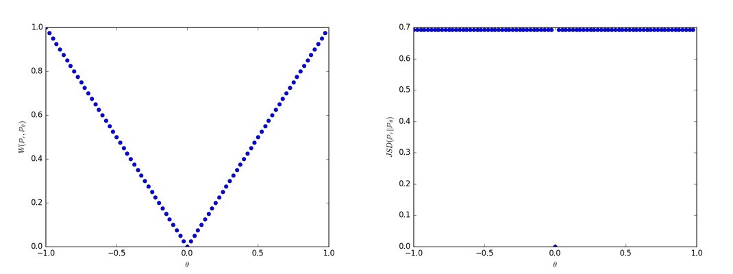
Figure 1: These plots show as a function of when is the EM distance (left plot) or the JS divergence (right plot). The EM plot is continuous and provides a usable gradient everywhere. The JS plot is not continuous and does not provide a usable gradient.
图 1:这些图给出 作为 的函数,其中 分别为 EM 距离(左)与 JS 散度(右)。EM 曲线连续,处处提供可用梯度;JS 曲线不连续,无法提供可用梯度。
Example 1 gives us a case where we can learn a probability distribution over a low dimensional manifold by doing gradient descent on the EM distance. This cannot be done with the other distances and divergences because the resulting loss function is not even continuous. Although this simple example features distributions with disjoint supports, the same conclusion holds when the supports have a non empty intersection contained in a set of measure zero. This happens to be the case when two low dimensional manifolds intersect in general position [1].
例 1 给出了一种情形:我们可以对 EM 距离做梯度下降,从而学习支撑在低维流形上的概率分布。对其他距离与散度则不行,因为得到的损失函数甚至不连续。尽管这个简单例子中分布支撑互不相交,但当支撑的非空交集落在零测集上时,同样结论成立。两条低维流形一般位置相交时正是如此 [1]。
Since the Wasserstein distance is much weaker than the JS distance[^3], we can now ask whether is a continuous loss function on under mild assumptions. This, and more, is true, as we now state and prove.
由于 Wasserstein 距离远弱于 JS 距离[^3],自然要问:在温和假设下, 是否关于 连续。这一点以及更多结论成立,我们陈述并证明如下。
Theorem 1.
Let be a fixed distribution over . Let be a random variable (e.g Gaussian) over another space . Let be a function, that will be denoted with the first coordinate and the second. Let denote the distribution of . Then,
定理 1。 设 为 上的固定分布。设 为另一空间 上的随机变量(例如高斯)。设 为函数,记第一坐标为 、第二坐标为 时写作 。令 表示 的分布。则
- Ifis continuous in, so is.
- 若关于连续,则亦连续。
- Ifis locally Lipschitz and satisfies regularity assumption*1, then*is continuous everywhere, and differentiable almost everywhere.
- 若局部 Lipschitz 且满足正则假设*1,则*处处连续,且几乎处处可微。
- Statements 1-2 are false for the Jensen-Shannon divergenceand all the KLs.
- 对 Jensen-Shannon 散度以及所有 KL,陈述 1–2 均不成立。
Proof.
See Appendix C ∎
证明。 见附录 C ∎
The following corollary tells us that learning by minimizing the EM distance makes sense (at least in theory) with neural networks.
下面的推论告诉我们:至少在理论上,用神经网络通过最小化 EM 距离来学习是说得通的。
Corollary 1.
Let be any feedforward neural network[^4] parameterized by , and a prior over such that (e.g. Gaussian, uniform, etc.). Then assumption 1 is satisfied and therefore is continuous everywhere and differentiable almost everywhere.
推论 1。 设 为任意由 参数化的前馈神经网络[^4], 为 上的先验且 (例如高斯、均匀等)。则假设 1 成立,因而 处处连续且几乎处处可微。
Proof.
See Appendix C ∎
证明。 见附录 C ∎
All this shows that EM is a much more sensible cost function for our problem than at least the Jensen-Shannon divergence. The following theorem describes the relative strength of the topologies induced by these distances and divergences, with KL the strongest, followed by JS and TV, and EM the weakest.
以上表明,至少相对 Jensen-Shannon 散度,EM 作为我们问题的代价函数合理得多。下面的定理描述这些距离与散度所诱导拓扑的相对强弱:KL 最强,其次是 JS 与 TV,EM 最弱。
Theorem 2.
Let be a distribution on a compact space and be a sequence of distributions on . Then, considering all limits as ,
定理 2。 设 为紧空间 上的分布, 为 上的分布序列。以下极限均指 时,
- The following statements are equivalent • withthe total variation distance. • withthe Jensen-Shannon divergence.
- 下列陈述等价 • ,为全变差距离。 • ,为 Jensen-Shannon 散度。
- The following statements are equivalent • . • whererepresents convergence in distribution for random variables.
- 下列陈述等价 • 。 • ,其中表示随机变量依分布收敛。
- orimply the statements in (1).
- 或蕴含 (1) 中的陈述。
- The statements in (1) imply the statements in (2).
- (1) 中的陈述蕴含 (2) 中的陈述。
Proof.
See Appendix C ∎
证明。 见附录 C ∎
This highlights the fact that the KL, JS, and TV distances are not sensible cost functions when learning distributions supported by low dimensional manifolds. However the EM distance is sensible in that setup. This obviously leads us to the next section where we introduce a practical approximation of optimizing the EM distance.
这说明:在学习支撑于低维流形的分布时,KL、JS 与 TV 距离都不是合理的代价函数;而 EM 距离在该设定下是合理的。这自然导向下一节:我们引入优化 EM 距离的实用近似。
3 Wasserstein GAN
Again, Theorem 2 points to the fact that might have nicer properties when optimized than . However, the infimum in (1) is highly intractable. On the other hand, the Kantorovich-Rubinstein duality [22] tells us that
再次地,定理 2 表明:优化 可能比优化 性质更好。然而 (1) 中的下确界极难计算。另一方面,Kantorovich-Rubinstein 对偶 [22] 告诉我们
where the supremum is over all the 1-Lipschitz functions . Note that if we replace for (consider -Lipschitz for some constant ), then we end up with . Therefore, if we have a parameterized family of functions that are all -Lipschitz for some , we could consider solving the problem
其中上确界取遍所有 1-Lipschitz 函数 。注意:若把 换成 (即考虑某个常数 的 -Lipschitz),则得到 。因此,若有参数化函数族 ,且它们对某个 全是 -Lipschitz,则可考虑求解问题
and if the supremum in (2) is attained for some (a pretty strong assumption akin to what’s assumed when proving consistency of an estimator), this process would yield a calculation of up to a multiplicative constant. Furthermore, we could consider differentiating (again, up to a constant) by back-proping through equation (2) via estimating . While this is all intuition, we now prove that this process is principled under the optimality assumption.
并且若 (2) 中的上确界在某个 处达到(这是相当强的假设,类似证明估计量一致性时所做的假定),该过程将得到 乘以某个常数因子的计算。进一步,我们还可通过估计 ,沿着方程 (2) 反向传播,从而对 (同样差一个常数因子)求导。以上全是直觉;下面我们证明:在最优性假设下,这一过程是有原理依据的。
Theorem 3.
Let be any distribution. Let be the distribution of with a random variable with density and a function satisfying assumption 1. Then, there is a solution to the problem
定理 3。 设 为任意分布。设 为 的分布,其中 有密度 ,且 满足假设 1。则问题
and we have
存在解 ,并且有
when both terms are well-defined.
在两项均有定义时成立。
Proof.
See Appendix Appendix C ∎
证明。 见附录 C ∎
Now comes the question of finding the function that solves the maximization problem in equation (2). To roughly approximate this, something that we can do is train a neural network parameterized with weights lying in a compact space and then backprop through , as we would do with a typical GAN. Note that the fact that is compact implies that all the functions will be -Lipschitz for some that only depends on and not the individual weights, therefore approximating (2) up to an irrelevant scaling factor and the capacity of the ‘critic’ . In order to have parameters lie in a compact space, something simple we can do is clamp the weights to a fixed box (say ) after each gradient update. The Wasserstein Generative Adversarial Network (WGAN) procedure is described in Algorithm 1.
接下来的问题是找出求解方程 (2) 最大化问题的函数 。粗略近似的做法是:训练权重落在紧集 上的神经网络,再对 反向传播,就像典型 GAN 那样。注意 紧意味着所有 对某个只依赖 、而不依赖个别权重的 都是 -Lipschitz,因而在差一个无关紧要的缩放因子以及「评判器」 容量的意义下近似 (2)。为使参数 落在紧集上,简单做法是每次梯度更新后把权重裁剪到固定盒子(例如 )。Wasserstein 生成对抗网络(WGAN)流程见算法 1。
Weight clipping is a clearly terrible way to enforce a Lipschitz constraint. If the clipping parameter is large, then it can take a long time for any weights to reach their limit, thereby making it harder to train the critic till optimality. If the clipping is small, this can easily lead to vanishing gradients when the number of layers is big, or batch normalization is not used (such as in RNNs). We experimented with simple variants (such as projecting the weights to a sphere) with little difference, and we stuck with weight clipping due to its simplicity and already good performance. However, we do leave the topic of enforcing Lipschitz constraints in a neural network setting for further investigation, and we actively encourage interested researchers to improve on this method.
用权重裁剪强制 Lipschitz 约束显然很粗糙。若裁剪参数过大,权重要很久才能碰到边界,评判器就更难训到最优;若裁剪过小,层数一多或不用批归一化(例如 RNN)时又容易梯度消失。我们试过简单变体(例如把权重投影到球面),差别不大,于是仍采用权重裁剪,因为它简单且已经表现不错。不过,如何在神经网络设定下更好强制 Lipschitz 约束,我们留给后续研究,并积极鼓励感兴趣的研究者改进这一方法。
1: : , the learning rate. , the clipping parameter. , the batch size. , the number of iterations of the critic per generator iteration.
2: : , initial critic parameters. , initial generator’s parameters.
3: while has not converged do
4: for do
5: Sample a batch from the real data.
6: Sample a batch of prior samples.
7:
8:
9:
10: end for
11: Sample a batch of prior samples.
12:
13:
14: end while
Algorithm 1 WGAN, our proposed algorithm. All experiments in the paper used the default values , , , .
1: :,学习率。,裁剪参数。,批大小。,每更新一次生成器时评判器的迭代次数。
2: :,评判器初始参数。,生成器初始参数。
3: while 尚未收敛 do
4: for do
5: 从真实数据采样一批 。
6: 从先验采样一批 。
7:
8:
9:
10: end for
11: 从先验采样一批 。
12:
13:
14: end while
算法 1 WGAN,本文提出的算法。文中所有实验使用默认值 ,,,。
The fact that the EM distance is continuous and differentiable a.e. means that we can (and should) train the critic till optimality. The argument is simple, the more we train the critic, the more reliable gradient of the Wasserstein we get, which is actually useful by the fact that Wasserstein is differentiable almost everywhere. For the JS, as the discriminator gets better the gradients get more reliable but the true gradient is 0 since the JS is locally saturated and we get vanishing gradients, as can be seen in Figure 1 of this paper and Theorem 2.4 of [1]. In Figure 2 we show a proof of concept of this, where we train a GAN discriminator and a WGAN critic till optimality. The discriminator learns very quickly to distinguish between fake and real, and as expected provides no reliable gradient information. The critic, however, can’t saturate, and converges to a linear function that gives remarkably clean gradients everywhere. The fact that we constrain the weights limits the possible growth of the function to be at most linear in different parts of the space, forcing the optimal critic to have this behaviour.
EM 距离连续且几乎处处可微,意味着我们可以(也应该)把评判器训到最优。理由很简单:评判器训得越充分,得到的 Wasserstein 梯度就越可靠;而 Wasserstein 几乎处处可微,这些梯度确实有用。对 JS 而言,判别器变好时梯度看起来更「可靠」,但真正的梯度是 0,因为 JS 局部饱和,会出现梯度消失,见图 1 以及 [1] 的定理 2.4。图 2 给出概念验证:把 GAN 判别器与 WGAN 评判器都训到最优。判别器很快学会区分真假,并如预期不再提供可靠梯度信息;评判器则无法饱和,收敛到在空间各处给出异常干净梯度的线性函数。权重受约束,使得函数在空间不同区域至多线性增长,从而迫使最优评判器呈现这种行为。
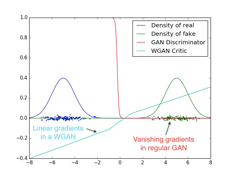
Figure 2: Optimal discriminator and critic when learning to differentiate two Gaussians. As we can see, the discriminator of a minimax GAN saturates and results in vanishing gradients. Our WGAN critic provides very clean gradients on all parts of the space.
图 2:区分两个高斯时的最优判别器与评判器。可见,minimax GAN 的判别器饱和并导致梯度消失;我们的 WGAN 评判器在空间各处都提供非常干净的梯度。
Perhaps more importantly, the fact that we can train the critic till optimality makes it impossible to collapse modes when we do. This is due to the fact that mode collapse comes from the fact that the optimal generator for a fixed discriminator is a sum of deltas on the points the discriminator assigns the highest values, as observed by [4] and highlighted in [11].
或许更重要的是:能够把评判器训到最优,使得在这种设定下不可能发生模式崩塌。原因在于:对固定判别器,最优生成器是判别器赋值最高的那些点上的 delta 之和,这一点由 [4] 观察到、并由 [11] 强调;模式崩塌正源于此。
In the following section we display the practical benefits of our new algorithm, and we provide an in-depth comparison of its behaviour and that of traditional GANs.
下一节展示新算法的实践收益,并深入比较它与传统 GAN 的行为。
4 Empirical Results
4 实验结果
We run experiments on image generation using our Wasserstein-GAN algorithm and show that there are significant practical benefits to using it over the formulation used in standard GANs.
我们用 Wasserstein-GAN 算法做图像生成实验,表明相对标准 GAN 的目标形式,它带来显著的实践收益。
We claim two main benefits:
我们声称两项主要收益:
- • a meaningful loss metric that correlates with the generator’s convergence and sample quality
- • 有意义的损失度量,与生成器收敛及样本质量相关
- • improved stability of the optimization process
- • 优化过程稳定性更好
4.1 Experimental Procedure
4.1 实验设定
We run experiments on image generation. The target distribution to learn is the LSUN-Bedrooms dataset [24] – a collection of natural images of indoor bedrooms. Our baseline comparison is DCGAN [18], a GAN with a convolutional architecture trained with the standard GAN procedure using the trick [4]. The generated samples are 3-channel images of 64x64 pixels in size. We use the hyper-parameters specified in Algorithm 1 for all of our experiments.
我们做图像生成实验。要学习的目标分布是 LSUN-Bedrooms 数据集 [24]——室内卧室自然图像集合。基线对照是 DCGAN [18],即以卷积架构、按标准 GAN 流程并用 技巧 [4] 训练的 GAN。生成样本为 64×64 像素的三通道图像。全部实验使用算法 1 中指定的超参数。
4.2 Meaningful loss metric
4.2 有意义的损失度量
Because the WGAN algorithm attempts to train the critic (lines 2–8 in Algorithm 1) relatively well before each generator update (line 10 in Algorithm 1), the loss function at this point is an estimate of the EM distance, up to constant factors related to the way we constrain the Lipschitz constant of .
由于 WGAN 算法在每次更新生成器(算法 1 第 10 行)之前,都尽量把评判器 (算法 1 第 2–8 行)训得较好,此时的损失函数就是 EM 距离的估计,至多差与约束 的 Lipschitz 常数相关的常数因子。
Our first experiment illustrates how this estimate correlates well with the quality of the generated samples. Besides the convolutional DCGAN architecture, we also ran experiments where we replace the generator or both the generator and the critic by 4-layer ReLU-MLP with 512 hidden units.
第一个实验说明该估计与生成样本质量相关性很好。除卷积 DCGAN 架构外,我们还把生成器、或生成器与评判器二者,替换为每层 512 隐单元的 4 层 ReLU-MLP,再跑实验。
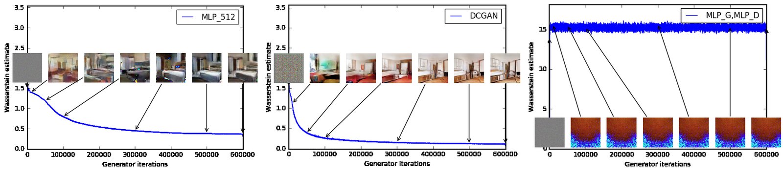
Figure 3: Training curves and samples at different stages of training. We can see a clear correlation between lower error and better sample quality. Upper left: the generator is an MLP with 4 hidden layers and 512 units at each layer. The loss decreases constistently as training progresses and sample quality increases. Upper right: the generator is a standard DCGAN. The loss decreases quickly and sample quality increases as well. In both upper plots the critic is a DCGAN without the sigmoid so losses can be subjected to comparison. Lower half: both the generator and the discriminator are MLPs with substantially high learning rates (so training failed). Loss is constant and samples are constant as well. The training curves were passed through a median filter for visualization purposes.
图 3:训练不同阶段的训练曲线与样本。可见误差越低、样本质量越好,相关清晰。左上:生成器为 4 隐层、每层 512 单元的 MLP。损失随训练持续下降,样本质量上升。右上:生成器为标准 DCGAN。损失快速下降,样本质量同样上升。两幅上图的评判器都是去掉 sigmoid 的 DCGAN,以便损失可比较。下半:生成器与判别器均为 MLP,学习率很高(因而训练失败)。损失几乎不变,样本也几乎不变。训练曲线经中值滤波以便可视化。
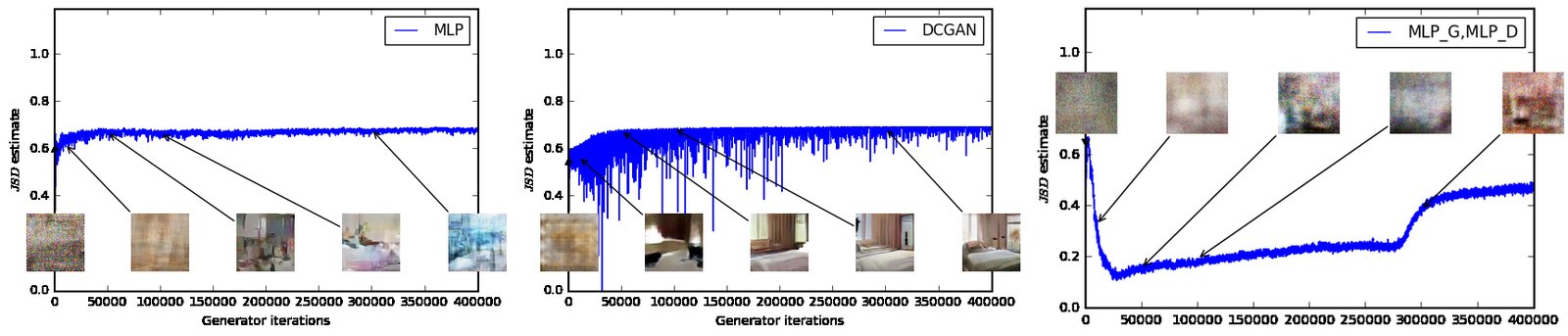
Figure 4: estimates for an MLP generator (upper left) and a DCGAN generator (upper right) trained with the standard GAN procedure. Both had a DCGAN discriminator. Both curves have increasing error. Samples get better for the DCGAN but the JS estimate increases or stays constant, pointing towards no significant correlation between sample quality and loss. Bottom: with both generator and discriminator. The curve goes up and down regardless of sample quality. All training curves were passed through the same median filter as in Figure 3.
图 4:用标准 GAN 流程训练时,MLP 生成器(左上)与 DCGAN 生成器(右上)的 估计;二者判别器均为 DCGAN。两条曲线误差都在上升。DCGAN 的样本变好,但 JS 估计上升或持平,说明样本质量与损失无明显相关。底部:生成器与判别器都是 MLP。曲线上下起伏,与样本质量无关。所有训练曲线使用与图 3 相同的中值滤波。
Figure 3plots the evolution of the WGAN estimate (3) of the EM distance during WGAN training for all three architectures. The plots clearly show that these curves correlate well with the visual quality of the generated samples.
图 3 画出三种架构在 WGAN 训练过程中,EM 距离的 WGAN 估计 (3) 如何演变。图清楚表明这些曲线与生成样本的视觉质量相关性很好。
To our knowledge, this is the first time in GAN literature that such a property is shown, where the loss of the GAN shows properties of convergence. This property is extremely useful when doing research in adversarial networks as one does not need to stare at the generated samples to figure out failure modes and to gain information on which models are doing better over others.
据我们所知,这是 GAN 文献中首次展示这种性质:GAN 的损失表现出收敛特征。对抗网络研究里这一点极为有用——不必盯着生成样本才能判断失败模式,也能比较哪些模型做得更好。
However, we do not claim that this is a new method to quantitatively evaluate generative models yet. The constant scaling factor that depends on the critic’s architecture means it’s hard to compare models with different critics. Even more, in practice the fact that the critic doesn’t have infinite capacity makes it hard to know just how close to the EM distance our estimate really is. This being said, we have succesfully used the loss metric to validate our experiments repeatedly and without failure, and we see this as a huge improvement in training GANs which previously had no such facility.
不过,我们并不声称这已经是定量评价生成模型的新方法。依赖评判器架构的常数缩放因子,使得不同评判器的模型难以横向比较。更进一步,实践中评判器容量有限,也很难说估计究竟离真正的 EM 距离有多近。尽管如此,我们已反复、无失败地用该损失度量验证实验,并视之为 GAN 训练的重大改进——此前完全没有这种便利。
In contrast, Figure 4 plots the evolution of the GAN estimate of the JS distance during GAN training. More precisely, during GAN training, the discriminator is trained to maximize
作为对照,图 4 画出 GAN 训练过程中 JS 距离的 GAN 估计如何演变。更精确地说,GAN 训练中判别器被训练以最大化
which is is a lower bound of . In the figure, we plot the quantity , which is a lower bound of the JS distance.
它是 的下界。图中我们画出量 ,它是 JS 距离的下界。
This quantity clearly correlates poorly the sample quality. Note also that the JS estimate usually stays constant or goes up instead of going down. In fact it often remains very close to which is the highest value taken by the JS distance. In other words, the JS distance saturates, the discriminator has zero loss, and the generated samples are in some cases meaningful (DCGAN generator, top right plot) and in other cases collapse to a single nonsensical image [4]. This last phenomenon has been theoretically explained in [1] and highlighted in [11].
该量与样本质量相关性明显很差。还要注意:JS 估计通常持平或上升,而不是下降。事实上它往往非常接近 ,即 JS 距离所能取的最大值。换句话说,JS 距离饱和,判别器损失为零;生成样本有时仍有意义(DCGAN 生成器,右上图),有时则崩塌成一张无意义图像 [4]。后一现象在 [1] 中有理论解释,并在 [11] 中被强调。
When using the trick [4], the discriminator loss and the generator loss are different. Figure 8 in Appendix E reports the same plots for GAN training, but using the generator loss instead of the discriminator loss. This does not change the conclusions.
使用 技巧 [4] 时,判别器损失与生成器损失不同。附录 E 的图 8 报告了同样的 GAN 训练图,但改用生成器损失而非判别器损失。结论不变。
Finally, as a negative result, we report that WGAN training becomes unstable at times when one uses a momentum based optimizer such as Adam [8] (with ) on the critic, or when one uses high learning rates. Since the loss for the critic is nonstationary, momentum based methods seemed to perform worse. We identified momentum as a potential cause because, as the loss blew up and samples got worse, the cosine between the Adam step and the gradient usually turned negative. The only places where this cosine was negative was in these situations of instability. We therefore switched to RMSProp [21] which is known to perform well even on very nonstationary problems [13].
最后,作为负面结果,我们报告:若对评判器使用基于动量的优化器如 Adam [8](且 ),或使用过高学习率,WGAN 训练有时会不稳定。由于评判器损失非平稳,基于动量的方法似乎表现更差。我们把动量视为可能原因,是因为当损失爆炸、样本变差时,Adam 步与梯度的余弦通常变为负值;该余弦为负的地方,恰恰就是这些不稳定情形。因此我们改用 RMSProp [21],它在非常非平稳的问题上也表现良好 [13]。
4.3 Improved stability
4.3 稳定性提升
One of the benefits of WGAN is that it allows us to train the critic till optimality. When the critic is trained to completion, it simply provides a loss to the generator that we can train as any other neural network. This tells us that we no longer need to balance generator and discriminator’s capacity properly. The better the critic, the higher quality the gradients we use to train the generator.
WGAN 的收益之一是允许把评判器训到最优。当评判器训充分后,它只是向生成器提供一个损失,我们便可像训练任何其他神经网络一样训练生成器。这说明不再需要恰当地平衡生成器与判别器的容量。评判器越好,用来训练生成器的梯度质量越高。
We observe that WGANs are much more robust than GANs when one varies the architectural choices for the generator. We illustrate this by running experiments on three generator architectures: (1) a convolutional DCGAN generator, (2) a convolutional DCGAN generator without batch normalization and with a constant number of filters, and (3) a 4-layer ReLU-MLP with 512 hidden units. The last two are known to perform very poorly with GANs. We keep the convolutional DCGAN architecture for the WGAN critic or the GAN discriminator.
我们观察到:改变生成器的架构选择时,WGAN 比 GAN 稳健得多。我们用三种生成器架构说明:(1) 卷积 DCGAN 生成器;(2) 去掉批归一化、滤波器数量恒定的卷积 DCGAN 生成器;(3) 每层 512 隐单元的 4 层 ReLU-MLP。后两种对 GAN 以表现很差著称。WGAN 评判器或 GAN 判别器则保持卷积 DCGAN 架构。

Figure 5: Algorithms trained with a DCGAN generator. Left: WGAN algorithm. Right: standard GAN formulation. Both algorithms produce high quality samples.
图 5:使用 DCGAN 生成器训练的算法。左:WGAN 算法。右:标准 GAN 形式。两种算法都产生高质量样本。
Figures 7, 7, and 7 show samples generated for these three architectures using both the WGAN and GAN algorithms. We refer the reader to Appendix Appendix F for full sheets of generated samples. Samples were not cherry-picked.
图 7、7 与 7 展示这三种架构分别用 WGAN 与 GAN 算法生成的样本。完整样本页见附录 F。样本未经挑拣。
In no experiment did we see evidence of mode collapse for the WGAN algorithm.
在任何实验中,我们都未看到 WGAN 算法出现模式崩塌的迹象。
5 Related Work
5 相关工作
There’s been a number of works on the so called Integral Probability Metrics (IPMs) [15]. Given a set of functions from to , we can define
所谓积分概率度量(Integral Probability Metrics, IPM)[15] 已有不少工作。给定从 到 的函数类 ,可定义
as an integral probability metric associated with the function class . It is easily verified that if for every we have (such as all examples we’ll consider), then is nonnegative, satisfies the triangular inequality, and is symmetric. Thus, is a pseudometric over .
为与函数类 相伴的积分概率度量。容易验证:若对每个 都有 (我们将考虑的例子皆如此),则 非负、满足三角不等式且对称。因此 是 上的伪度量。
While IPMs might seem to share a similar formula, as we will see different classes of functions can yeald to radically different metrics.
尽管 IPM 看起来公式相近,我们将看到:不同的函数类会给出截然不同的度量。
- • By the Kantorovich-Rubinstein duality [22], we know that when is the set of 1-Lipschitz functions. Furthermore, if is the set of -Lipschitz functions, we get .
- • 由 Kantorovich-Rubinstein 对偶 [22],当 为 1-Lipschitz 函数全体时,。进一步,若 为 -Lipschitz 函数全体,则 。
- • When is the set of all measurable functions bounded between -1 and 1 (or all continuous functions between -1 and 1), we retrieve the total variation distance [15]. This already tells us that going from 1-Lipschitz to 1-Bounded functions drastically changes the topology of the space, and the regularity of as a loss function (as by Theorems 1 and 2).
- • 当 为取值介于 与 的全体可测函数(或介于 与 的全体连续函数)时,得到 ,即全变差距离 [15]。这说明从 1-Lipschitz 换成 1-有界函数会剧烈改变空间拓扑,以及 作为损失函数的正则性(见定理 1 与 2)。
- • Energy-based GANs (EBGANs) [25] can be thought of as the generative approach to the total variation distance. This connection is stated and proven in depth in Appendix Appendix D. At the core of the connection is that the discriminator will play the role of maximizing equation (4) while its only restriction is being between and for some constant . This will yeald the same behaviour as being restricted to be between and up to a constant scaling factor irrelevant to optimization. Thus, when the discriminator approaches optimality the cost for the generator will aproximate the total variation distance . Since the total variation distance displays the same regularity as the JS, it can be seen that EBGANs will suffer from the same problems of classical GANs regarding not being able to train the discriminator till optimality and thus limiting itself to very imperfect gradients.
- • 基于能量的 GAN(EBGAN)[25] 可视为全变差距离的生成式做法。这一联系在附录 D 中有完整陈述与证明。核心在于:判别器扮演最大化方程 (4) 中 的角色,其唯一限制是取值介于 与某个常数 之间。这与限制在 与 之间行为相同,只差一个对优化无关紧要的常数缩放。因此当判别器接近最优时,生成器的代价会近似全变差距离 。由于全变差与 JS 具有相同的正则性,可见 EBGAN 会遭受与经典 GAN 同样的问题:无法把判别器训到最优,从而只能拿到非常不完美的梯度。
- • Maximum Mean Discrepancy (MMD) [5] is a specific case of integral probability metrics when for some Reproducing Kernel Hilbert Space (RKHS) associated with a given kernel . As proved on [5] we know that MMD is a proper metric and not only a pseudometric when the kernel is universal. In the specific case where for the normalized Lebesgue measure on , we know that will be contained in , and therefore so the regularity of the MMD distance as a loss function will be at least as bad as the one of the total variation. Nevertheless this is a very extreme case, since we would need a very powerful kernel to approximate the whole . However, even Gaussian kernels are able to detect tiny noise patterns as recently evidenced by [20]. This points to the fact that especially with low bandwidth kernels, the distance might be close to a saturating regime similar as with total variation or the JS. This obviously doesn’t need to be the case for every kernel, and figuring out how and which different MMDs are closer to Wasserstein or total variation distances is an interesting topic of research. The great aspect of MMD is that via the kernel trick there is no need to train a separate network to maximize equation (4) for the ball of a RKHS. However, this has the disadvantage that evaluating the MMD distance has computational cost that grows quadratically with the amount of samples used to estimate the expectations in (4). This last point makes MMD have limited scalability, and is sometimes inapplicable to many real life applications because of it. There are estimates with linear computational cost for the MMD [5] which in a lot of cases makes MMD very useful, but they also have worse sample complexity.
- • 最大均值差异(Maximum Mean Discrepancy, MMD)[5] 是积分概率度量的特例:取 ,其中 为与给定核 相伴的再生核希尔伯特空间(RKHS)。[5] 证明:当核普遍(universal)时,MMD 是真正的度量而非仅伪度量。在 、 为 上归一化 Lebesgue 测度这一特例中, 含于 ,因而 ,于是 MMD 作为损失函数的正则性至少与全变差一样差。不过这是极端情形,因为需要很强的核才能逼近整个 。即便高斯核也能检测极细微的噪声模式,[20] 最近的证据即是。这说明尤其在低带宽核下,该距离可能接近类似全变差或 JS 的饱和区间。当然并非每个核都会如此;弄清不同 MMD 如何更接近 Wasserstein 或全变差,是有趣的研究方向。MMD 的一大优点是:借助核技巧,不必另训网络去最大化 RKHS 球上的方程 (4)。缺点是:估计 MMD 的计算代价随用于估计 (4) 中期望的样本数二次增长。这使 MMD 可扩展性受限,有时因代价过高而不适用于许多实际问题。存在计算代价线性于样本数的 MMD 估计 [5],很多情形下很有用,但样本复杂度更差。
- • Generative Moment Matching Networks (GMMNs) [10, 2] are the generative counterpart of MMD. By backproping through the kernelized formula for equation (4), they directly optimize (the IPM when is as in the previous item). As mentioned, this has the advantage of not requiring a separate network to approximately maximize equation (4). However, GMMNs have enjoyed limited applicability. Partial explanations for their unsuccess are the quadratic cost as a function of the number of samples and vanishing gradients for low-bandwidth kernels. Furthermore, it may be possible that some kernels used in practice are unsuitable for capturing very complex distances in high dimensional sample spaces such as natural images. This is properly justified by the fact that [19] shows that for the typical Gaussian MMD test to be reliable (as in it’s power as a statistical test approaching 1), we need the number of samples to grow linearly with the number of dimensions. Since the MMD computational cost grows quadratically with the number of samples in the batch used to estimate equation (4), this makes the cost of having a reliable estimator grow quadratically with the number of dimensions, which makes it very inapplicable for high dimensional problems. Indeed, for something as standard as x images, we would need minibatches of size at least (without taking into account the constants in the bounds of [19] which would make this number substantially larger) and a total cost per iteration of , over 5 orders of magnitude more than a GAN iteration when using the standard batch size of 64. That being said, these numbers can be a bit unfair to the MMD, in the sense that we are comparing empirical sample complexity of GANs with the theoretical sample complexity of MMDs, which tends to be worse. However, in the original GMMN paper [10] they indeed used a minibatch of size 1000, much larger than the standard 32 or 64 (even when this incurred in quadratic computational cost). While estimates that have linear computational cost as a function of the number of samples exist [5], they have worse sample complexity, and to the best of our knowledge they haven’t been yet applied in a generative context such as in GMMNs.
- • 生成矩匹配网络(Generative Moment Matching Networks, GMMN)[10, 2] 是 MMD 的生成式对应。通过对方程 (4) 的核化公式反向传播,它们直接优化 (即 如上一项时的 IPM)。如前所述,优点是不必另训网络近似最大化 (4)。然而 GMMN 应用有限。部分解释包括:代价随样本数二次增长,以及低带宽核下的梯度消失。此外,实践中使用的某些核可能不适合刻画自然图像等高维样本空间中的复杂距离。[19] 表明:要使典型高斯 MMD 检验可靠(功效趋于 1),样本数需随维数线性增长。由于估计 (4) 的 MMD 计算代价随批内样本数二次增长,可靠估计器的代价将随维数二次增长,对高维问题很不实用。的确,对标准的 图像,至少需要大小为 的小批量(尚未计入 [19] 界中的常数,那些常数会使该数字显著更大),每步总代价 ,比标准批大小 64 的 GAN 迭代高出五个数量级以上。当然,这些数字对 MMD 可能略欠公允:我们是在用 GAN 的经验样本复杂度对照 MMD 的理论样本复杂度,后者往往更差。不过原 GMMN 论文 [10] 确实使用大小 1000 的小批量,远大于标准的 32 或 64(即便这会带来二次计算代价)。虽存在对样本数线性代价的估计 [5],但样本复杂度更差,且据我们所知尚未用于类似 GMMN 的生成设定。
On another great line of research, the recent work of [14] has explored the use of Wasserstein distances in the context of learning for Restricted Boltzmann Machines for discrete spaces. The motivations at a first glance might seem quite different, since the manifold setting is restricted to continuous spaces and in finite discrete spaces the weak and strong topologies (the ones of W and JS respectively) coincide. However, in the end there is more in commmon than not about our motivations. We both want to compare distributions in a way that leverages the geometry of the underlying space, and Wasserstein allows us to do exactly that.
另一条重要研究线是 [14] 近期的工作:在离散空间上把 Wasserstein 距离用于受限玻尔兹曼机的学习。乍看动机似乎很不同,因为流形设定限于连续空间,而在有限离散空间上弱拓扑与强拓扑(分别对应 W 与 JS)重合。不过归根结底,双方动机的共同点多于差异。我们都希望以利用底层空间几何的方式比较分布,而 Wasserstein 恰好允许我们这样做。
Finally, the work of [3] shows new algorithms for calculating Wasserstein distances between different distributions. We believe this direction is quite important, and perhaps could lead to new ways of evaluating generative models.
最后,[3] 给出计算不同分布之间 Wasserstein 距离的新算法。我们认为这一方向相当重要,或许能带来评价生成模型的新途径。
6 Conclusion
6 结论
We introduced an algorithm that we deemed WGAN, an alternative to traditional GAN training. In this new model, we showed that we can improve the stability of learning, get rid of problems like mode collapse, and provide meaningful learning curves useful for debugging and hyperparameter searches. Furthermore, we showed that the corresponding optimization problem is sound, and provided extensive theoretical work highlighting the deep connections to other distances between distributions.
我们引入称为 WGAN 的算法,作为传统 GAN 训练的替代。在这一新模型中,我们表明可以改善学习稳定性、摆脱模式崩塌等问题,并提供对调试与超参搜索有用的、有意义的学习曲线。此外,我们说明相应优化问题可靠,并给出大量理论工作,突出它与其他分布间距离的深层联系。
Acknowledgments
致谢
We would like to thank Mohamed Ishmael Belghazi, Emily Denton, Ian Goodfellow, Ishaan Gulrajani, Alex Lamb, David Lopez-Paz, Eric Martin, Maxime Oquab, Aditya Ramesh, Ronan Riochet, Uri Shalit, Pablo Sprechmann, Arthur Szlam, Ruohan Wang, for helpful comments and advice.
感谢 Mohamed Ishmael Belghazi、Emily Denton、Ian Goodfellow、Ishaan Gulrajani、Alex Lamb、David Lopez-Paz、Eric Martin、Maxime Oquab、Aditya Ramesh、Ronan Riochet、Uri Shalit、Pablo Sprechmann、Arthur Szlam、Ruohan Wang 提供有益评论与建议。
References
参考文献
[1] Martin Arjovsky and Léon Bottou. Towards principled methods for training generative adversarial networks. In International Conference on Learning Representations , 2017. Under review.
[2] Gintare Karolina Dziugaite, Daniel M. Roy, and Zoubin Ghahramani. Training generative neural networks via maximum mean discrepancy optimization. CoRR , abs/1505.03906, 2015.
[3] Aude Genevay, Marco Cuturi, Gabriel Peyré, and Francis Bach. Stochastic optimization for large-scale optimal transport. In D. D. Lee, M. Sugiyama, U. V. Luxburg, I. Guyon, and R. Garnett, editors, Advances in Neural Information Processing Systems 29 , pages 3440–3448. Curran Associates, Inc., 2016.
[4] Ian J. Goodfellow, Jean Pouget-Abadie, Mehdi Mirza, Bing Xu, David Warde-Farley, Sherjil Ozair, Aaron Courville, and Yoshua Bengio. Generative adversarial nets. In Advances in Neural Information Processing Systems 27 , pages 2672–2680. Curran Associates, Inc., 2014.
[5] Arthur Gretton, Karsten M. Borgwardt, Malte J. Rasch, Bernhard Schölkopf, and Alexander Smola. A kernel two-sample test. J. Mach. Learn. Res. , 13:723–773, 2012.
[6] Ferenc Huszar. How (not) to train your generative model: Scheduled sampling, likelihood, adversary? CoRR , abs/1511.05101, 2015.
[7] Shizuo Kakutani. Concrete representation of abstract (m)-spaces (a characterization of the space of continuous functions). Annals of Mathematics , 42(4):994–1024, 1941.
[8] Diederik P. Kingma and Jimmy Ba. Adam: A method for stochastic optimization. CoRR , abs/1412.6980, 2014.
[9] Diederik P. Kingma and Max Welling. Auto-encoding variational bayes. CoRR , abs/1312.6114, 2013.
[10] Yujia Li, Kevin Swersky, and Rich Zemel. Generative moment matching networks. In Proceedings of the 32nd International Conference on Machine Learning (ICML-15) , pages 1718–1727. JMLR Workshop and Conference Proceedings, 2015.
[11] Luke Metz, Ben Poole, David Pfau, and Jascha Sohl-Dickstein. Unrolled generative adversarial networks. Corr , abs/1611.02163, 2016.
[12] Paul Milgrom and Ilya Segal. Envelope theorems for arbitrary choice sets. Econometrica , 70(2):583–601, 2002.
[13] Volodymyr Mnih, Adrià Puigdomènech Badia, Mehdi Mirza, Alex Graves, Timothy P. Lillicrap, Tim Harley, David Silver, and Koray Kavukcuoglu. Asynchronous methods for deep reinforcement learning. In Proceedings of the 33nd International Conference on Machine Learning, ICML 2016, New York City, NY, USA, June 19-24, 2016 , pages 1928–1937, 2016.
[14] Grégoire Montavon, Klaus-Robert Müller, and Marco Cuturi. Wasserstein training of restricted boltzmann machines. In D. D. Lee, M. Sugiyama, U. V. Luxburg, I. Guyon, and R. Garnett, editors, Advances in Neural Information Processing Systems 29 , pages 3718–3726. Curran Associates, Inc., 2016.
[15] Alfred Müller. Integral probability metrics and their generating classes of functions. Advances in Applied Probability , 29(2):429–443, 1997.
[16] Radford M. Neal. Annealed importance sampling. Statistics and Computing , 11(2):125–139, April 2001.
[17] Sebastian Nowozin, Botond Cseke, and Ryota Tomioka. f-gan: Training generative neural samplers using variational divergence minimization. pages 271–279, 2016.
[18] Alec Radford, Luke Metz, and Soumith Chintala. Unsupervised representation learning with deep convolutional generative adversarial networks. CoRR , abs/1511.06434, 2015.
[19] Aaditya Ramdas, Sashank J. Reddi, Barnabas Poczos, Aarti Singh, and Larry Wasserman. On the high-dimensional power of linear-time kernel two-sample testing under mean-difference alternatives. Corr , abs/1411.6314, 2014.
[20] Dougal J Sutherland, Hsiao-Yu Tung, Heiko Strathmann, Soumyajit De, Aaditya Ramdas, Alex Smola, and Arthur Gretton. Generative models and model criticism via optimized maximum mean discrepancy. In International Conference on Learning Representations , 2017. Under review.
[21] T. Tieleman and G. Hinton. Lecture 6.5—RmsProp: Divide the gradient by a running average of its recent magnitude. COURSERA: Neural Networks for Machine Learning, 2012.
[22] Cédric Villani. Optimal Transport: Old and New . Grundlehren der mathematischen Wissenschaften. Springer, Berlin, 2009.
[23] Yuhuai Wu, Yuri Burda, Ruslan Salakhutdinov, and Roger B. Grosse. On the quantitative analysis of decoder-based generative models. CoRR , abs/1611.04273, 2016.
[24] Fisher Yu, Yinda Zhang, Shuran Song, Ari Seff, and Jianxiong Xiao. LSUN: Construction of a large-scale image dataset using deep learning with humans in the loop. Corr , abs/1506.03365, 2015.
[25] Junbo Zhao, Michael Mathieu, and Yann LeCun. Energy-based generative adversarial network. Corr , abs/1609.03126, 2016.
Appendix A Why Wasserstein is indeed weak
附录 A 为何 Wasserstein 确实更弱
We now introduce our notation. Let be a compact set (such as the space of images). We define to be the space of probability measures over . We note
先约定记号。设 为紧集(例如图像空间 )。定义 为 上的概率测度空间。记
Note that if , we can define , since is bounded. With this norm, the space is a normed vector space. As for any normed vector space, we can define its dual
注意:若 ,可定义 ,因为 有界。配备该范数后, 为赋范向量空间。对任意赋范向量空间,可定义其对偶
$C_{b}(\mathcal{X})^{*}=\{\phi:C_{b}(\mathcal{X})\rightarrow\mathbb{R}\text{,\phi$ is linear
and continuous}}$$
and give it the dual norm .
并赋予对偶范数 。
With this definitions, is another normed space. Now let be a signed measure over , and let us define the total variation distance
在这些定义下, 又是一个赋范空间。现设 为 上的符号测度,定义全变差距离
where the supremum is taken all Borel sets in . Since the total variation is a norm, then if we have and two probability distributions over ,
其中上确界取遍 的全体 Borel 集。由于全变差是范数,若 与 为 上的两个概率分布,则
is a distance in (called the total variation distance).
是 上的距离(称为全变差距离)。
We can consider
我们可以考虑
where is a linear function over . The Riesz Representation theorem ([7], Theorem 10) tells us that is an isometric immersion. This tells us that we can effectively consider with the total variation distance as a subset of with the norm distance. Thus, just to accentuate it one more time, the total variation over is exactly the norm distance over .
其中 是 上的线性泛函。Riesz 表示定理([7],定理 10)告诉我们 是等距浸入。这意味着我们可以有效地把配备全变差距离的 视为配备范数距离的 的子集。因此,再强调一次: 上的全变差恰好是 上的范数距离。
Let us stop for a second and analyze what all this technicality meant. The main thing to carry is that we introduced a distance over probability distributions. When looked as a distance over a subset of , this distance gives the norm topology. The norm topology is very strong. Therefore, we can expect that not many functions will be continuous when measuring distances between distributions with . As we will show later in Theorem 2, gives the same topology as the Jensen-Shannon divergence, pointing to the fact that the JS is a very strong distance, and is thus more propense to give a discontinuous loss function.
停下来分析这些技术细节意味着什么。要带走的主要一点是:我们在概率分布上引入了距离 。当把它看作 子集上的距离时,该距离给出范数拓扑。范数拓扑非常强。因此可以预期:用 度量分布间距离时,不会有很多函数 连续。后面定理 2 将表明 与 Jensen-Shannon 散度给出相同拓扑,说明 JS 是很强的距离,因而更容易给出不连续的损失函数。
Now, all dual spaces (such as and thus ) have a strong topology (induced by the norm), and a weak* topology. As the name suggests, the weak* topology is much weaker than the strong topology. In the case of , the strong topology is given by the total variation distance, and the weak* topology is given by the Wasserstein distance (among others) [22].
所有对偶空间(例如 ,因而也包括 )都有强拓扑(由范数诱导)与弱* 拓扑。顾名思义,弱* 拓扑远弱于强拓扑。对 ,强拓扑由全变差距离给出,弱* 拓扑则由 Wasserstein 距离(以及其他若干距离)给出 [22]。
Appendix B Assumption definitions
附录 B 假设的定义
Assumption 1.
Let be locally Lipschitz between finite dimensional vector spaces. We will denote it’s evaluation on coordinates . We say that satisfies assumption 1 for a certain probability distribution over if there are local Lipschitz constants such that
假设 1。 设 为有限维向量空间之间的局部 Lipschitz 映射。在坐标 上的取值记为 。若存在局部 Lipschitz 常数 使得
Appendix C Proofs of things
附录 C 证明
Proof of Theorem 1.
Let and be two parameter vectors in . Then, we will first attempt to bound , from where the theorem will come easily. The main element of the proof is the use of the coupling , the distribution of the joint , which clearly has .
定理 1 的证明。 设 与 为 中两个参数向量。我们先尝试界住 ,定理将由此容易得出。证明的关键要素是使用耦合 ,即联合 的分布,显然 。
By the definition of the Wasserstein distance, we have
由 Wasserstein 距离的定义,有
If is continuous in , then , so pointwise as functions of . Since is compact, the distance of any two elements in it has to be uniformly bounded by some constant , and therefore for all and uniformly. By the bounded convergence theorem, we therefore have
若 关于 连续,则 ,因而 作为 的函数逐点趋于 0。由于 紧,其中任意两点距离被某常数 一致上界,故对所有 与 一致有 。由有界收敛定理,因而有
Finally, we have that
最后,我们有
proving the continuity of .
从而证明了 的连续性。
Now let be locally Lipschitz. Then, for a given pair there is a constant and an open set such that , such that for every we have
现设 局部 Lipschitz。则对给定对 ,存在常数 与开集 使 ,且对每个 有
By taking expectations and we
取期望并令 ,得到
whenever . Therefore, we can define . It’s easy to see that since was open, is as well. Furthermore, by assumption 1, we can define and achieve
只要 。因此可定义 。易见因 开, 亦开。进一步,由假设 1,可定义 ,并得到
for all , meaning that is locally Lipschitz. This obviously implies that is everywhere continuous, and by Radamacher’s theorem we know it has to be differentiable almost everywhere.
对所有 成立,意味着 局部 Lipschitz。这显然蕴含 处处连续;由 Rademacher 定理,它几乎处处可微。
The counterexample for item 3 of the Theorem is indeed Example 1. ∎
定理第 3 项的反例正是例 1。∎
Proof of Corollary 1.
We begin with the case of smooth nonlinearities. Since is as a function of then for any fixed we have is an acceptable local Lipschitz constant for all . Therefore, it suffices to prove
推论 1 的证明。 先考虑光滑非线性。由于 作为 的函数属于 ,对任意固定 , 对所有 都是可接受的局部 Lipschitz 常数。因此只需证明
If is the number of layers we know that where are the weight matrices and is are the diagonal Jacobians of the nonlinearities. Let be the application of layers to inclusively (e.g. ). Then, . We recall that if is the Lipschitz constant of the nonlinearity, then and . Putting this together,
若 为层数,则知 ,其中 为权矩阵, 为非线性的对角雅可比。令 表示第 到 层(含)的复合(例如 )。则 。我们回忆:若 为非线性的 Lipschitz 常数,则 且 。合在一起,
If and then
若 且 ,则
finishing the proof ∎
证毕 ∎
Proof of Theorem 2.
定理 2 的证明。
- • () — Let be the mixture distribution (note that depends on ). It is easily verified that , and in particular this tends to 0 (as does ). We now show this for completeness. Let be a signed measure, we define . for all Borel sets . In this case, Let be the Radon-Nykodim derivative between and the mixture. Note that by construction for every Borel set we have . If then we get which implies . This means that is bounded by 3 (and therefore and )-almost everywhere. We could have done this for any constant larger than 2 but for our purposes 3 will sufice. Let fixed, and . Then, Therefore, Which implies . Furthermore, We now can see that Taking limsup we get for all , which means . In the same way, we can define , and meaning that and therefore is bounded by 3 almost everywhere for and . With the same calculation, and so , and therefore . We can now show so we achieve and then . Finally, we conclude • () — by a simple application of the triangular and Pinsker’s inequalities we get
- • () — 令 为混合分布 (注意 依赖 )。容易验证 ,因而它趋于 0( 亦然)。为完整起见我们写出证明。设 为符号测度,定义 ,上确界取遍所有 Borel 集 。此时, 。令 为 关于混合分布的 Radon-Nikodym 导数。由构造,对每个 Borel 集 有 。若 ,则 ,从而 。这意味着 在 (因而也在 与 )几乎处处被 3 上界。对任意大于 2 的常数本也可做同样论证,对我们的目的取 3 已足够。固定 ,令 。则 。因此 。于是 。进一步, 。于是可见 。取 limsup 得对所有 有 ,故 。同理可定义 ,且 ,意味着 ,因而 对 、 与 几乎处处被 3 上界。同样计算:,且 ,故 ,从而 。现可证 ,于是 ,进而 。最后得出 。 • () — 由三角不等式与 Pinsker 不等式的简单应用得 。
- This is a long known fact that metrizes the weak* topology of on , and by definition this is the topology of convergence in distribution. A proof of this can be found (for example) in [22].
- 这是久为人知的事实: 在 上度量化 的弱* 拓扑,而依定义这正是依分布收敛的拓扑。证明例如可见 [22]。
- This is a straightforward application of Pinsker’s inequality
- 这是 Pinsker 不等式的直接应用
- This is trivial by recalling the fact that and give the strong and weak* topologies on the dual of when restricted to .
- 这是平凡的:只需回忆 与 在限制到 时,分别给出 对偶上的强拓扑与弱* 拓扑。
∎
Proof of Theorem 3.
Let us define
定理 3 的证明。 定义
where lies in \mathcal{F}=\{\tilde{f}:\mathcal{X}\to\mathbb{R}\text{ ,\tilde{f}\in C_{b}(\mathcal{X})|\tilde{f}|_{L}\leq 1}\} and .
其中 属于 \mathcal{F}=\{\tilde{f}:\mathcal{X}\to\mathbb{R}\text{ ,\tilde{f}\in C_{b}(\mathcal{X})|\tilde{f}|_{L}\leq 1}\},且 。
Since is compact, we know by the Kantorovich-Rubenstein duality [22] that there is an that attains the value
由于 紧,由 Kantorovich-Rubinstein 对偶 [22] 知存在 达到
Let us define . By the above point we know then that is non-empty. We know that by a simple envelope theorem ([12], Theorem 1) that
定义 。由上知 非空。由简单的包络定理([12],定理 1)知
for any when both terms are well-defined.
对任意 ,在两项均有定义时成立。
Let , which we knows exists since is non-empty for all . Then, we get
取 (因对所有 , 非空,故知其存在)。则有
under the condition that the first and last terms are well-defined. The rest of the proof will be dedicated to show that
前提是首末两项均有定义。证明的其余部分将表明
when the right hand side is defined. For the reader who is not interested in such technicalities, he or she can skip the rest of the proof.
在右端有定义时成立。对不关心此类技术细节的读者,可跳过余下证明。
Since , we know that it is 1-Lipschitz. Furthermore, is locally Lipschitz as a function of . Therefore, is locally Lipschitz on with constants (the same ones as ). By Radamacher’s Theorem, has to be differentiable almost everywhere for jointly. Rewriting this, the set A=\{(\theta,z):\text{f\circ gis not differentiable}\} has measure 0. By Fubini’s Theorem, this implies that for almost every the section has measure 0. Let’s now fix a such that the measure of is null (such as when the right hand side of equation (5) is well defined). For this we have is well-defined for almost any , and since has a density, it is defined -a.e. By assumption 1 we know that
由于 ,知其为 1-Lipschitz。又 作为 的函数局部 Lipschitz。因此 在 上局部 Lipschitz,常数为 (与 相同)。由 Rademacher 定理, 对 联合几乎处处可微。换言之,集合 A=\{(\theta,z):\text{f\circ g不可微}\} 测度为 0。由 Fubini 定理,对几乎所有 ,截面 测度为 0。现固定使 测度为零的 (例如当方程 (5) 右端有定义时)。对该 , 对几乎所有 有定义;又因 有密度,它在 -几乎处处有定义。由假设 1 知
so is well-defined for almost every . Now, we can see
故 对几乎所有 有定义。于是可见
By differentiability, the term inside the integral converges -a.e. to 0 as . Furthermore,
由可微性,积分号内的项在 时 -几乎处处收敛到 0。进一步,
$$|\frac{f(g_{\theta}(z))-f(g_{\theta_{0}}(z))-\langle(\theta-\theta_{0}),\nabla_{\theta}f(g_{\theta}(z))|{\theta{0}}\rangle}{|\theta-\theta_{0}|}|\
\leq\frac{|\theta-\theta_{0}|L(\theta_{0},z)+|\theta-\theta_{0}||\nabla_{\theta}f(g_{\theta}(z))|{\theta{0}}|}{|\theta-\theta_{0}|}\
\leq 2L(\theta_{0},z)$$
and since by assumption 1, we get by dominated convergence that Equation 6 converges to 0 as so
又因由假设 1 有 ,由控制收敛定理,方程 6 在 时收敛到 0,于是
for almost every , and in particular when the right hand side is well defined. Note that the mere existance of the left hand side (meaning the differentiability a.e. of ) had to be proven, which we just did. ∎
对几乎所有 成立,尤其是在右端有定义时。注意:左端的存在性本身(即 几乎处处可微)也需要证明,而我们刚刚完成了这一点。∎
Appendix D Energy-based GANs optimize total variation
附录 D 基于能量的 GAN 优化的是全变差
In this appendix we show that under an optimal discriminator, energy-based GANs (EBGANs) [25] optimize the total variation distance between the real and generated distributions.
本附录说明:在最优判别器下,基于能量的 GAN(EBGAN)[25] 优化的是真实分布与生成分布之间的全变差距离。
Energy-based GANs are trained in a similar fashion to GANs, only under a different loss function. They have a discriminator who tries to minimize
基于能量的 GAN 训练方式类似 GAN,只是损失函数不同。它们有一个判别器 ,试图最小化
for some and and a generator network that’s trained to minimize
其中 ,;生成网络 被训练以最小化
Very importantly, is constrained to be non-negative, since otherwise the trivial solution for would be to set everything to arbitrarily low values. The original EBGAN paper used only for the loss of the generator, but this is obviously equivalent to our definition since the term does not dependent on for a fixed discriminator (such as when backproping to the generator in EBGAN training) and thus minimizing one or the other is equivalent.
极为重要的是: 被约束为非负,否则 的平凡解会是把一切设为任意低的值。原 EBGAN 论文生成器损失只用 ,但这显然与我们的定义等价,因为对固定判别器(例如在 EBGAN 训练中反向传播到生成器时)项 不依赖 ,最小化其一或另一等价。
We say that a measurable function is optimal for (or if for all other measurable functions . We show that such a discriminator always exists for any two distributions and , and that under such a discriminator, is proportional to . As a simple corollary, we get the fact that attains its minimum value if and only if is at its minimum value, which is 0, and (Theorems 1-2 of [25]).
称可测函数 对 (或 )最优,若对所有其他可测函数 都有 。我们证明:对任意两个分布 与 这样的判别器总存在;且在该判别器下, 与 成比例。作为简单推论, 取到最小值当且仅当 取到最小值 0,且 ([25] 定理 1–2)。
Theorem 4.
Let be a the real data distribution over a compact space . Let be a measurable function (such as any neural network). Then, an optimal discriminator $D^{}\mathbb{P}{r}\mathbb{P}{\theta}$, and*
定理 4。 设 为紧空间 上的真实数据分布。设 为可测函数(例如任意神经网络)。则对 与 存在最优判别器 $D^{}$,且*
Proof.
First, we prove that there exists an optimal discriminator. Let be a measurable function, then is also a measurable function, and . Therefore, a function is optimal if and only if is. Furthermore, it is optimal if and only if for all . We are then interested to see if there’s an optimal discriminator for the problem .
证明。 首先证明最优判别器存在。设 可测,则 亦可测,且 。因此 最优当且仅当 最优。进一步,它最优当且仅当对所有 有 。于是我们关心问题 是否有最优判别器。
Note now that if we have
注意:若 ,则有
Therefore, we know that
因此可知
The interesting part is that
有趣的是
and there is an such that . This is a long known fact, found for example in [22], but we prove it later for completeness. In that case, we define . We then have and
且存在 使 。这是久为人知的事实,例如见 [22],但为完整起见我们稍后证明。此时定义 。则 ,且
This shows that is optimal and . Furthermore,
这说明 最优,且 。进一步,
concluding the proof.
证毕。
For completeness, we now show a proof for equation (7) and the existence of said that attains the value of the infimum. Take , which is a signed measure, and its Hahn decomposition. Then, we can define . By construction, then
为完整起见,我们现给出方程 (7) 以及达到下确界的所述 存在性的证明。取 ,它是符号测度,并取 为其 Hahn 分解。则可定义 。由构造,
Furthermore, if is bounded between -1 and 1, we get
进一步,若 介于 与 之间,则有
Since is positive, we can conclude . ∎
由于 为正,可结论 。∎
Appendix E Generator’s cost during normal GAN training
附录 E 普通 GAN 训练中生成器的代价
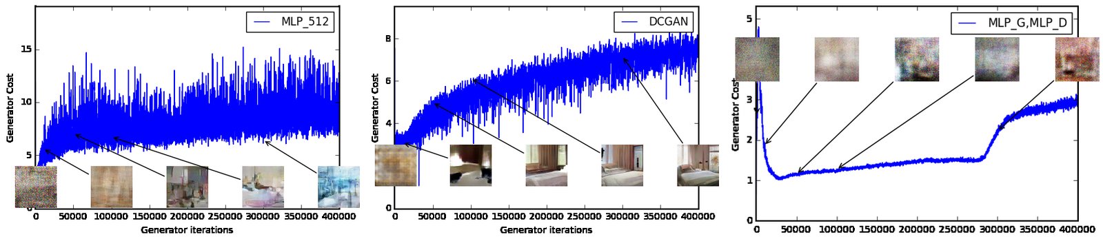
Figure 8: Cost of the generator during normal GAN training, for an MLP generator (upper left) and a DCGAN generator (upper right). Both had a DCGAN discriminator. Both curves have increasing error. Samples get better for the DCGAN but the cost of the generator increases, pointing towards no significant correlation between sample quality and loss. Bottom: with both generator and discriminator. The curve goes up and down regardless of sample quality. All training curves were passed through the same median filter as in Figure 3.
图 8:普通 GAN 训练中生成器的代价:MLP 生成器(左上)与 DCGAN 生成器(右上);二者判别器均为 DCGAN。两条曲线误差都在上升。DCGAN 的样本变好,但生成器代价上升,说明样本质量与损失无明显相关。底部:生成器与判别器都是 MLP。曲线上下起伏,与样本质量无关。所有训练曲线使用与图 3 相同的中值滤波。
Appendix F Sheets of samples
附录 F 样本图页
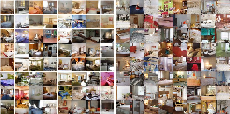
Figure 9: WGAN algorithm: generator and critic are DCGANs.
图 9:WGAN 算法:生成器与评判器均为 DCGAN。
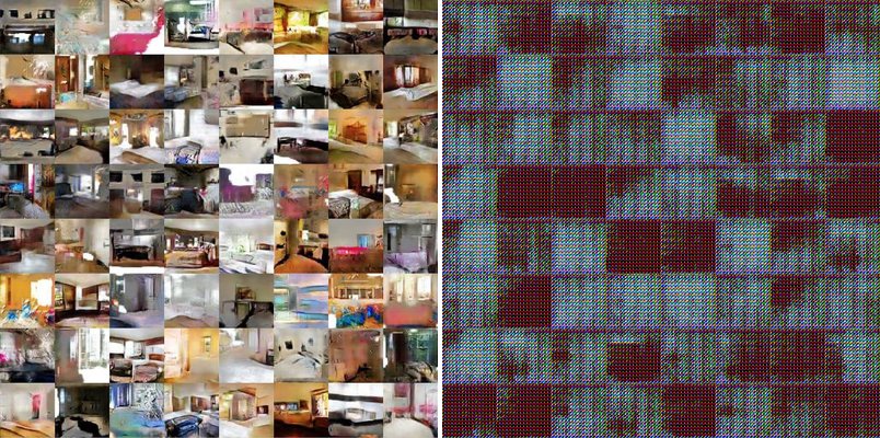
Figure 11: WGAN algorithm: generator is a DCGAN without batchnorm and constant filter size. Critic is a DCGAN.
图 11:WGAN 算法:生成器为去掉批归一化、滤波器大小恒定的 DCGAN;评判器为 DCGAN。
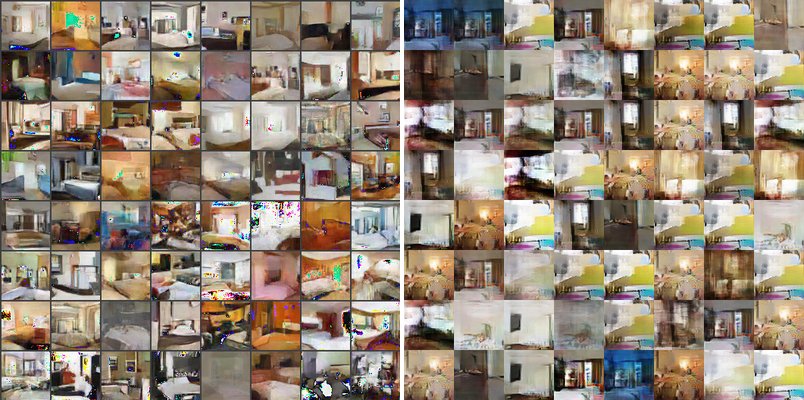
Figure 13: WGAN algorithm: generator is an MLP with 4 hidden layers of 512 units, critic is a DCGAN.
图 13:WGAN 算法:生成器为 4 隐层、每层 512 单元的 MLP;评判器为 DCGAN。