Neural Discrete Representation Learning

神经离散表征学习

Aaron van den Oord Affiliation:  DeepMind Email:  avdnoord@google.com    Oriol Vinyals Affiliation:  DeepMind Email:  vinyals@google.com    Koray Kavukcuoglu Affiliation:  DeepMind Email:  korayk@google.com

Abstract

摘要

Learning useful representations without supervision remains a key challenge in machine learning. In this paper, we propose a simple yet powerful generative model that learns such discrete representations. Our model, the Vector Quantised-Variational AutoEncoder (VQ-VAE), differs from VAEs in two key ways: the encoder network outputs discrete, rather than continuous, codes; and the prior is learnt rather than static. In order to learn a discrete latent representation, we incorporate ideas from vector quantisation (VQ). Using the VQ method allows the model to circumvent issues of “posterior collapse” -— where the latents are ignored when they are paired with a powerful autoregressive decoder -— typically observed in the VAE framework. Pairing these representations with an autoregressive prior, the model can generate high quality images, videos, and speech as well as doing high quality speaker conversion and unsupervised learning of phonemes, providing further evidence of the utility of the learnt representations.

在无监督条件下学到有用表征，至今仍是机器学习的核心难题之一。本文提出一种简洁却有力的生成模型，专门学习离散表征。该模型称为向量量化变分自编码器（Vector Quantised-Variational AutoEncoder，VQ-VAE），与普通 VAE 有两处关键不同：编码器输出离散码而非连续码；先验由学习得到而非固定。为学习离散潜变量，我们引入向量量化（vector quantisation，VQ）的思想。借助 VQ，模型可绕开「后验坍塌」——即潜变量与强大自回归解码器配对时被忽略——这一在 VAE 框架中常见的问题。把这些表征再配上自回归先验，模型能够生成高质量图像、视频与语音，也能完成高质量说话人转换，以及无监督地学习音素，进一步说明所学表征确有用处。

1 Introduction

1 引言

Recent advances in generative modelling of images [38, 12, 13, 22, 10], audio [37, 26] and videos [20, 11] have yielded impressive samples and applications [24, 18]. At the same time, challenging tasks such as few-shot learning [34], domain adaptation [17], or reinforcement learning [35] heavily rely on learnt representations from raw data, but the usefulness of generic representations trained in an unsupervised fashion is still far from being the dominant approach.

图像 [38, 12, 13, 22, 10]、音频 [37, 26] 与视频 [20, 11] 生成建模近年进展显著，样本质量与应用 [24, 18] 都很可观。与此同时，少样本学习 [34]、域适应 [17]、强化学习 [35] 等难题高度依赖从原始数据学到的表征，但无监督训出的通用表征，距离成为主流做法仍有一段距离。

Maximum likelihood and reconstruction error are two common objectives used to train unsupervised models in the pixel domain, however their usefulness depends on the particular application the features are used in. Our goal is to achieve a model that conserves the important features of the data in its latent space while optimising for maximum likelihood. As the work in [7] suggests, the best generative models (as measured by log-likelihood) will be those without latents but a powerful decoder (such as PixelCNN). However, in this paper, we argue for learning discrete and useful latent variables, which we demonstrate on a variety of domains.

极大似然与重建误差是像素域无监督训练的两类常用目标，其效用取决于特征最终用在何处。我们的目标是：在优化极大似然的同时，让潜空间保住数据中的重要特征。如 [7] 所指出，按对数似然衡量，最好的生成模型往往没有潜变量，而是配一个强大解码器（如 PixelCNN）。本文则主张学习离散且有用的潜变量，并在多个模态上给出实证。

Learning representations with continuous features have been the focus of many previous work [16, 39, 6, 9] however we concentrate on discrete representations [27, 33, 8, 28] which are potentially a more natural fit for many of the modalities we are interested in. Language is inherently discrete, similarly speech is typically represented as a sequence of symbols. Images can often be described concisely by language [40]. Furthermore, discrete representations are a natural fit for complex reasoning, planning and predictive learning (e.g., if it rains, I will use an umbrella). While using discrete latent variables in deep learning has proven challenging, powerful autoregressive models have been developed for modelling distributions over discrete variables [37].

连续特征表征已有大量工作 [16, 39, 6, 9]；我们关注离散表征 [27, 33, 8, 28]，它往往更贴合我们关心的模态。语言本身就是离散的，语音也常被表示成符号序列；图像常常可用语言简洁描述 [40]。离散表征也更适合复杂推理、规划与预测学习（例如：如果下雨，我就带伞）。尽管在深度学习中使用离散潜变量一向困难，但针对离散变量分布的强大自回归模型已经出现 [37]。

In our work, we introduce a new family of generative models succesfully combining the variational autoencoder (VAE) framework with discrete latent representations through a novel parameterisation of the posterior distribution of (discrete) latents given an observation. Our model, which relies on vector quantization (VQ), is simple to train, does not suffer from large variance, and avoids the “posterior collapse” issue which has been problematic with many VAE models that have a powerful decoder, often caused by latents being ignored. Additionally, it is the first discrete latent VAE model that get similar performance as its continuous counterparts, while offering the flexibility of discrete distributions. We term our model the VQ-VAE.

本文引入一类新的生成模型：通过新颖地参数化「给定观测的离散潜变量后验」，把变分自编码器（VAE）框架与离散潜表征成功结合起来。该模型依赖向量量化（VQ），训练简单，方差不大，并能避免许多配有强解码器的 VAE 常见的「后验坍塌」——往往是因为潜变量被忽略。此外，它是首个在性能上可与连续潜变量版本比肩、同时又保留离散分布灵活性的离散潜变量 VAE。我们称之为 VQ-VAE。

Since VQ-VAE can make effective use of the latent space, it can successfully model important features that usually span many dimensions in data space (for example objects span many pixels in images, phonemes in speech, the message in a text fragment, etc.) as opposed to focusing or spending capacity on noise and imperceptible details which are often local.

由于 VQ-VAE 能有效利用潜空间，它更擅长刻画在数据空间中往往跨越许多维度的重要特征（例如图像中占许多像素的物体、语音中的音素、文本片段中的信息等），而不是把容量耗在噪声与局部难察觉的细节上。

Lastly, once a good discrete latent structure of a modality is discovered by the VQ-VAE, we train a powerful prior over these discrete random variables, yielding interesting samples and useful applications. For instance, when trained on speech we discover the latent structure of language without any supervision or prior knowledge about phonemes or words. Furthermore, we can equip our decoder with the speaker identity, which allows for speaker conversion, i.e., transferring the voice from one speaker to another without changing the contents. We also show promising results on learning long term structure of environments for RL.

最后，一旦 VQ-VAE 发现了某模态良好的离散潜结构，我们再在这些离散随机变量上训练强大先验，即可得到有趣样本与实用应用。例如，在语音上训练时，无需任何监督或关于音素、词的先验知识，就能发现语言的潜结构；再给解码器配上说话人身份，即可做说话人转换——把一人的声音换成另一人，而不改内容。我们也在强化学习环境的长期结构学习上看到了有希望的结果。

Our contributions can thus be summarised as:

贡献可概括为：

• • Introducing the VQ-VAE model, which is simple, uses discrete latents, does not suffer from “posterior collapse” and has no variance issues.
• • We show that a discrete latent model (VQ-VAE) perform as well as its continuous model counterparts in log-likelihood.
• • When paired with a powerful prior, our samples are coherent and high quality on a wide variety of applications such as speech and video generation.
• • We show evidence of learning language through raw speech, without any supervision, and show applications of unsupervised speaker conversion.

• • 提出 VQ-VAE：结构简单、使用离散潜变量、不受「后验坍塌」困扰，也没有严重方差问题。
• • 表明离散潜变量模型（VQ-VAE）在对数似然上可与连续潜变量对应物相当。
• • 配上强大先验后，在语音、视频生成等广泛应用上样本连贯且质量高。
• • 给出从原始语音无监督地「学到语言」的证据，并展示无监督说话人转换应用。

2 Related Work

2 相关工作

In this work we present a new way of training variational autoencoders [23, 32] with discrete latent variables [27]. Using discrete variables in deep learning has proven challenging, as suggested by the dominance of continuous latent variables in most of current work – even when the underlying modality is inherently discrete.

本文给出一种用离散潜变量训练变分自编码器 [23, 32] 的新方法 [27]。在深度学习中使用离散变量一向困难——即便底层模态本身就是离散的，当前工作大多仍以连续潜变量为主，也可由此看出。

There exist many alternatives for training discrete VAEs. The NVIL [27] estimator use a single-sample objective to optimise the variational lower bound, and uses various variance-reduction techniques to speed up training. VIMCO [28] optimises a multi-sample objective [5], which speeds up convergence further by using multiple samples from the inference network.

训练离散 VAE 已有多种替代方案。NVIL [27] 估计器用单样本目标优化变分下界，并借助多种降方差技巧加速训练；VIMCO [28] 优化多样本目标 [5]，通过从推断网络采多个样本进一步加快收敛。

Recently a few authors have suggested the use of a new continuous reparemetrisation based on the so-called Concrete [25] or Gumbel-softmax [19] distribution, which is a continuous distribution and has a temperature constant that can be annealed during training to converge to a discrete distribution in the limit. In the beginning of training the variance of the gradients is low but biased, and towards the end of training the variance becomes high but unbiased.

近来也有工作提出基于所谓 Concrete [25] 或 Gumbel-softmax [19] 分布的连续重参数化：这是一类连续分布，带有可在训练中退火的温度常数，极限下收敛到离散分布。训练初期梯度方差低但有偏，末期方差变高但无偏。

None of the above methods, however, close the performance gap of VAEs with continuous latent variables where one can use the Gaussian reparameterisation trick which benefits from much lower variance in the gradients. Furthermore, most of these techniques are typically evaluated on relatively small datasets such as MNIST, and the dimensionality of the latent distributions is small (e.g., below 8). In our work, we use three complex image datasets (CIFAR10, ImageNet, and DeepMind Lab) and a raw speech dataset (VCTK).

然而上述方法都未能弥合与连续潜变量 VAE 的性能差距——后者可用高斯重参数化技巧，梯度方差低得多。而且这些技术多在 MNIST 等相对小数据集上评估，潜分布维度也较小（例如低于 8）。本文使用三个复杂图像数据集（CIFAR10、ImageNet、DeepMind Lab）以及原始语音数据集（VCTK）。

Our work also extends the line of research where autoregressive distributions are used in the decoder of VAEs and/or in the prior [14]. This has been done for language modelling with LSTM decoders [4], and more recently with dilated convolutional decoders [42]. PixelCNNs [29, 38] are convolutional autoregressive models which have also been used as distribution in the decoder of VAEs [15, 7].

本文也延续了在 VAE 解码器与/或先验中使用自回归分布的研究线 [14]：语言建模上有 LSTM 解码器 [4]，近来也有膨胀卷积解码器 [42]；PixelCNN [29, 38] 作为卷积自回归模型，也被用作 VAE 解码器中的分布 [15, 7]。

Finally, our approach also relates to work in image compression with neural networks. Theis et. al. [36] use scalar quantisation to compress activations for lossy image compression before arithmetic encoding. Other authors [1] propose a method for similar compression model with vector quantisation. The authors propose a continuous relaxation of vector quantisation which is annealed over time to obtain a hard clustering. In their experiments they first train an autoencoder, afterwards vector quantisation is applied to the activations of the encoder, and finally the whole network is fine tuned using the soft-to-hard relaxation with a small learning rate. In our experiments we were unable to train using the soft-to-hard relaxation approach from scratch as the decoder was always able to invert the continuous relaxation during training, so that no actual quantisation took place.

最后，我们的方法也与神经网络图像压缩相关。Theis 等人 [36] 在算术编码前对激活做标量量化，用于有损图像压缩；另有工作 [1] 提出类似压缩模型，但用向量量化，并给出一种向量量化的连续松弛，随时间退火以得到硬聚类。他们先训自编码器，再对编码器激活做向量量化，最后用 soft-to-hard 松弛与小学习率微调整网。我们的实验中，无法从零开始用 soft-to-hard 松弛训练：解码器总能在训练中反演该连续松弛，以至于实际上没有发生量化。

3 VQ-VAE

Perhaps the work most related to our approach are VAEs. VAEs consist of the following parts: an encoder network which parameterises a posterior distribution $q(z|x)$ of discrete latent random variables $z$ given the input data $x$, a prior distribution $p(z)$, and a decoder with a distribution $p(x|z)$ over input data.

与本文最相关的或许就是 VAE。VAE 包含：参数化后验分布 $q(z|x)$ 的编码器网络（给定输入数据 $x$ 的离散潜随机变量 $z$）、先验 $p(z)$，以及输入数据上的解码器分布 $p(x|z)$。

Typically, the posteriors and priors in VAEs are assumed normally distributed with diagonal covariance, which allows for the Gaussian reparametrisation trick to be used [32, 23]. Extensions include autoregressive prior and posterior models [14], normalising flows [31, 10], and inverse autoregressive posteriors [22].

VAE 中后验与先验通常假定为对角协方差的正态分布，以便使用高斯重参数化技巧 [32, 23]。扩展包括自回归先验与后验 [14]、归一化流 [31, 10]，以及逆自回归后验 [22]。

In this work we introduce the VQ-VAE where we use discrete latent variables with a new way of training, inspired by vector quantisation (VQ). The posterior and prior distributions are categorical, and the samples drawn from these distributions index an embedding table. These embeddings are then used as input into the decoder network.

本文引入 VQ-VAE：使用离散潜变量，并以受向量量化（VQ）启发的新方式训练。后验与先验均为类别分布，从中采样得到的样本用于索引嵌入表；这些嵌入再作为解码器网络的输入。

3.1 Discrete Latent variables

3.1 离散潜变量

We define a latent embedding space $e\in R^{K\times D}$ where $K$ is the size of the discrete latent space (i.e., a $K$-way categorical), and $D$ is the dimensionality of each latent embedding vector $e_{i}$. Note that there are $K$ embedding vectors $e_{i}\in R^{D}$, $i\in{1,2,...,K}$. As shown in Figure 1, the model takes an input $x$, that is passed through an encoder producing output $z_{e}(x)$. The discrete latent variables $z$ are then calculated by a nearest neighbour look-up using the shared embedding space $e$ as shown in equation 1. The input to the decoder is the corresponding embedding vector $e_{k}$ as given in equation 2. One can see this forward computation pipeline as a regular autoencoder with a particular non-linearity that maps the latents to $1$-of-K embedding vectors. The complete set of parameters for the model are union of parameters of the encoder, decoder, and the embedding space $e$. For sake of simplicity we use a single random variable $z$ to represent the discrete latent variables in this Section, however for speech, image and videos we actually extract a 1D, 2D and 3D latent feature spaces respectively.

定义潜嵌入空间 $e\in R^{K\times D}$，其中 $K$ 是离散潜空间大小（即 $K$ 类类别分布），$D$ 是每个潜嵌入向量 $e_{i}$ 的维数。共有 $K$ 个嵌入向量 $e_{i}\in R^{D}$，$i\in\{1,2,...,K\}$。如图 1 所示，模型接受输入 $x$，经编码器得到输出 $z_{e}(x)$；离散潜变量 $z$ 再通过对共享嵌入空间 $e$ 做最近邻查找得到，见式 (1)；解码器输入为对应嵌入向量 $e_{k}$，见式 (2)。可以把这条前向计算管线看成普通自编码器，只是带有一种把潜变量映射到 1-of-K 嵌入向量的特殊非线性。模型完整参数集是编码器、解码器与嵌入空间 $e$ 参数的并集。本节为简便用单个随机变量 $z$ 表示离散潜变量；对语音、图像与视频，我们实际分别提取一维、二维与三维潜特征空间。

The posterior categorical distribution $q(z|x)$ probabilities are defined as one-hot as follows:

后验类别分布 $q(z|x)$ 的概率定义为如下 one-hot：

$q(z=k|x)=\begin{cases}1&\text{for } k = \text{argmin}{}{j}|z{e}(x)-e_{j}|_{2}$,\
0&\text{otherwise}\end{cases}, \tag{1}$$

where $z_{e}(x)$ is the output of the encoder network. We view this model as a VAE in which we can bound $\log p(x)$ with the ELBO. Our proposal distribution $q(z=k|x)$ is deterministic, and by defining a simple uniform prior over $z$ we obtain a KL divergence constant and equal to $\log K$.

其中 $z_{e}(x)$ 是编码器网络的输出。我们把该模型视为可用 ELBO 下界 $\log p(x)$ 的 VAE。提议分布 $q(z=k|x)$ 是确定性的；若对 $z$ 取简单均匀先验，则 KL 散度为常数且等于 $\log K$。

The representation $z_{e}(x)$ is passed through the discretisation bottleneck followed by mapping onto the nearest element of embedding $e$ as given in equations 1 and 2.

表示 $z_{e}(x)$ 经过离散化瓶颈，再映射到嵌入 $e$ 的最近元素，如式 (1) 与 (2) 所示。

$$z_{q}(x)=e_{k},\quad\text{where}\quad k=\text{argmin}_{j}\|z_{e}(x)-e_{j}\|_{2} \tag{2}$$

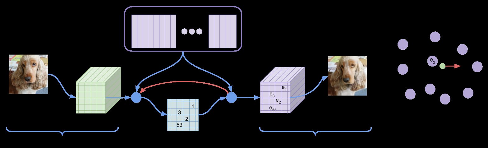
Figure 1: Left: A figure describing the VQ-VAE. Right: Visualisation of the embedding space. The output of the encoder $z(x)$ is mapped to the nearest point $e_{2}$. The gradient $\nabla_{z}L$ (in red) will push the encoder to change its output, which could alter the configuration in the next forward pass.

图 1：左：VQ-VAE 结构示意。右：嵌入空间可视化。编码器输出 $z(x)$ 被映射到最近点 $e_{2}$。梯度 $\nabla_{z}L$（红色）会推动编码器改变输出，从而可能改变下一次前向传播中的配置。

3.2 Learning

3.2 学习

Note that there is no real gradient defined for equation 2, however we approximate the gradient similar to the straight-through estimator [3] and just copy gradients from decoder input $z_{q}(x)$ to encoder output $z_{e}(x)$. One could also use the subgradient through the quantisation operation, but this simple estimator worked well for the initial experiments in this paper.

注意式 (2) 没有真正定义好的梯度；我们采用类似直通估计器 [3] 的近似，把解码器输入 $z_{q}(x)$ 上的梯度直接拷贝到编码器输出 $z_{e}(x)$。也可使用量化运算的次梯度，但在本文初步实验中，这一简单估计器已够用。

During forward computation the nearest embedding $z_{q}(x)$ (equation 2) is passed to the decoder, and during the backwards pass the gradient $\nabla_{z}L$ is passed unaltered to the encoder. Since the output representation of the encoder and the input to the decoder share the same $D$ dimensional space, the gradients contain useful information for how the encoder has to change its output to lower the reconstruction loss.

前向计算时，最近嵌入 $z_{q}(x)$（式 2）送入解码器；反向传播时，梯度 $\nabla_{z}L$ 原样传给编码器。由于编码器输出表示与解码器输入共享同一 $D$ 维空间，这些梯度包含「编码器应如何改输出以降低重建损失」的有用信息。

As seen on Figure 1 (right), the gradient can push the encoder’s output to be discretised differently in the next forward pass, because the assignment in equation 1 will be different.

如图 1（右）所示，梯度可推动编码器输出在下一次前向中被离散化到不同位置，因为式 (1) 的赋值会改变。

Equation 3 specifies the overall loss function. It is has three components that are used to train different parts of VQ-VAE. The first term is the reconstruction loss (or the data term) which optimizes the decoder and the encoder (through the estimator explained above). Due to the straight-through gradient estimation of mapping from $z_{e}(x)$ to $z_{q}(x)$, the embeddings $e_{i}$ receive no gradients from the reconstruction loss $\log p(z|z_{q}(x))$. Therefore, in order to learn the embedding space, we use one of the simplest dictionary learning algorithms, Vector Quantisation (VQ). The VQ objective uses the $l_{2}$ error to move the embedding vectors $e_{i}$ towards the encoder outputs $z_{e}(x)$ as shown in the second term of equation 3. Because this loss term is only used for updating the dictionary, one can alternatively also update the dictionary items as function of moving averages of $z_{e}(x)$ (not used for the experiments in this work). For more details see Appendix A.1.

式 (3) 给出总损失函数，含三项，分别训练 VQ-VAE 的不同部分。第一项是重建损失（数据项），优化解码器与编码器（经上述估计器）。由于从 $z_{e}(x)$ 到 $z_{q}(x)$ 的映射使用直通梯度估计，嵌入 $e_{i}$ 从重建损失 $\log p(x|z_{q}(x))$ 收不到梯度。因此，为学习嵌入空间，我们采用最简单的字典学习算法之一——向量量化（VQ）。VQ 目标用 $l_{2}$ 误差把嵌入向量 $e_{i}$ 拉向编码器输出 $z_{e}(x)$，见式 (3) 第二项。该项只用于更新字典，也可改用 $z_{e}(x)$ 的滑动平均来更新字典项（本文实验未采用）；细节见附录 A.1。

Finally, since the volume of the embedding space is dimensionless, it can grow arbitrarily if the embeddings $e_{i}$ do not train as fast as the encoder parameters. To make sure the encoder commits to an embedding and its output does not grow, we add a commitment loss, the third term in equation 3. Thus, the total training objective becomes:

最后，嵌入空间的「体积」无量纲，若嵌入 $e_{i}$ 训练跟不上编码器参数，体积可能任意增大。为确保编码器承诺某个嵌入且其输出不膨胀，我们加入承诺损失，即式 (3) 第三项。于是总训练目标为：

$$L=\log p(x|z_{q}(x))+\|\text{sg}[z_{e}(x)]-e\|^{2}_{2}+\beta\|z_{e}(x)-\text{sg}[e]\|^{2}_{2}, \tag{3}$$

where sg stands for the stopgradient operator that is defined as identity at forward computation time and has zero partial derivatives, thus effectively constraining its operand to be a non-updated constant. The decoder optimises the first loss term only, the encoder optimises the first and the last loss terms, and the embeddings are optimised by the middle loss term. We found the resulting algorithm to be quite robust to $\beta$, as the results did not vary for values of $\beta$ ranging from $0.1$ to $2.0$. We use $\beta=0.25$ in all our experiments, although in general this would depend on the scale of reconstruction loss. Since we assume a uniform prior for $z$, the KL term that usually appears in the ELBO is constant w.r.t. the encoder parameters and can thus be ignored for training.

其中 sg 表示 stopgradient 算子：前向为恒等，偏导为零，从而把其操作数约束为不更新的常数。解码器只优化第一项；编码器优化第一项与最后一项；嵌入由中间项优化。我们发现算法对 $\beta$ 相当稳健：$\beta$ 从 $0.1$ 到 $2.0$ 结果变化不大。全部实验取 $\beta=0.25$，一般而言这取决于重建损失的尺度。由于对 $z$ 假定均匀先验，ELBO 中通常出现的 KL 项相对编码器参数为常数，训练时可忽略。

In our experiments we define $N$ discrete latents (e.g., we use a field of 32 x 32 latents for ImageNet, or 8 x 8 x 10 for CIFAR10). The resulting loss $L$ is identical, except that we get an average over $N$ terms for $k$-means and commitment loss – one for each latent.

实验中我们定义 $N$ 个离散潜变量（例如 ImageNet 用 $32\times 32$ 潜场，CIFAR10 用 $8\times 8\times 10$）。损失 $L$ 形式相同，只是对 k-means 与承诺损失多了在 $N$ 项上的平均——每个潜变量一项。

The log-likelihood of the complete model $\log p(x)$ can be evaluated as follows:

完整模型的对数似然 $\log p(x)$ 可如下求值：

$$\log p(x)=\log\sum_{k}p(x|z_{k})p(z_{k}),$$

Because the decoder $p(x|z)$ is trained with $z=z_{q}(x)$ from MAP-inference, the decoder should not allocate any probability mass to $p(x|z)$ for $z\neq z_{q}(x)$ once it has fully converged. Thus, we can write $\log p(x)\approx\log p(x|z_{q}(x))p(z_{q}(x))$. We empirically evaluate this approximation in section 4. From Jensen’s inequality, we also can write $\log p(x)\geq\log p(x|z_{q}(x))p(z_{q}(x))$.

因为解码器 $p(x|z)$ 是在 MAP 推断给出的 $z=z_{q}(x)$ 上训练的，充分收敛后解码器不应再把概率质量分给 $z\neq z_{q}(x)$ 的 $p(x|z)$。于是可写 $\log p(x)\approx\log p(x|z_{q}(x))p(z_{q}(x))$。第 4 节经验评估该近似。由 Jensen 不等式也可写 $\log p(x)\geq\log p(x|z_{q}(x))p(z_{q}(x))$。

3.3 Prior

3.3 先验

The prior distribution over the discrete latents $p(z)$ is a categorical distribution, and can be made autoregressive by depending on other $z$ in the feature map. Whilst training the VQ-VAE, the prior is kept constant and uniform. After training, we fit an autoregressive distribution over $z$, $p(z)$, so that we can generate $x$ via ancestral sampling. We use a PixelCNN over the discrete latents for images, and a WaveNet for raw audio. Training the prior and the VQ-VAE jointly, which could strengthen our results, is left as future research.

离散潜变量上的先验 $p(z)$ 是类别分布，也可通过依赖特征图中其他 $z$ 做成自回归。训练 VQ-VAE 时先验保持常数均匀；训练结束后，再在 $z$ 上拟合自回归分布 $p(z)$，以便通过祖先采样生成 $x$。图像用离散潜变量上的 PixelCNN，原始音频用 WaveNet。联合训练先验与 VQ-VAE 可能进一步强化结果，留作未来工作。

4 Experiments

4 实验

4.1 Comparison with continuous variables

4.1 与连续变量的比较

As a first experiment we compare VQ-VAE with normal VAEs (with continuous variables), as well as VIMCO [28] with independent Gaussian or categorical priors. We train these models using the same standard VAE architecture on CIFAR10, while varying the latent capacity (number of continuous or discrete latent variables, as well as the dimensionality of the discrete space K). The encoder consists of 2 strided convolutional layers with stride 2 and window size $4\times 4$, followed by two residual $3\times 3$ blocks (implemented as ReLU, 3x3 conv, ReLU, 1x1 conv), all having 256 hidden units. The decoder similarly has two residual $3\times 3$ blocks, followed by two transposed convolutions with stride 2 and window size $4\times 4$. We use the ADAM optimiser [21] with learning rate 2e-4 and evaluate the performance after 250,000 steps with batch-size 128. For VIMCO we use 50 samples in the multi-sample training objective.

首个实验将 VQ-VAE 与普通 VAE（连续变量）以及带独立高斯或类别先验的 VIMCO [28] 比较。在 CIFAR10 上用同一标准 VAE 架构训练，同时改变潜容量（连续或离散潜变量个数，以及离散空间维数 $K$）。编码器含两个步长为 2、窗口 $4\times 4$ 的跨步卷积，再接两个残差 $3\times 3$ 块（实现为 ReLU、$3\times 3$ 卷积、ReLU、$1\times 1$ 卷积），隐单元均为 256。解码器对称：两个残差 $3\times 3$ 块，再接两个步长 2、窗口 $4\times 4$ 的转置卷积。优化器用 ADAM [21]，学习率 2e-4，batch-size 128，训练 250,000 步后评估。VIMCO 多样本训练目标使用 50 个样本。

The VAE, VQ-VAE and VIMCO models obtain 4.51 bits/dim, 4.67 bits/dim and 5.14 respectively. All reported likelihoods are lower bounds. Our numbers for the continuous VAE are comparable to those reported for a Deep convolutional VAE: 4.54 bits/dim [13] on this dataset.

VAE、VQ-VAE 与 VIMCO 分别得到 4.51 bits/dim、4.67 bits/dim 与 5.14。所报似然均为下界。连续 VAE 的数字与该数据集上 Deep convolutional VAE 所报 4.54 bits/dim [13] 相当。

Our model is the first among those using discrete latent variables which challenges the performance of continuous VAEs. Thus, we get very good reconstructions like regular VAEs provide, with the compressed representation that symbolic representations provide. A few interesting characteristics, implications and applications of the VQ-VAEs that we train is shown in the next subsections.

在使用离散潜变量的模型中，我们的模型是首个能挑战连续 VAE 性能的。因此既能像普通 VAE 那样得到很好的重建，又具备符号表征所带来的压缩表示。下一小节展示所训 VQ-VAE 的若干有趣特性、含义与应用。

4.2 Images

4.2 图像

Images contain a lot of redundant information as most of the pixels are correlated and noisy, therefore learning models at the pixel level could be wasteful.

图像含大量冗余：多数像素相关且嘈杂，因此在像素级建模可能浪费。

In this experiment we show that we can model $x=128\times 128\times 3$ images by compressing them to a $z=32\times 32\times 1$ discrete space (with K=512) via a purely deconvolutional $p(x|z)$. So a reduction of $\frac{128\times 128\times 3\times 8}{32\times 32\times 9}\approx 42.6$ in bits. We model images by learning a powerful prior (PixelCNN) over $z$. This allows to not only greatly speed up training and sampling, but also to use the PixelCNNs capacity to capture the global structure instead of the low-level statistics of images.

本实验表明，可把 $x=128\times 128\times 3$ 图像经纯反卷积 $p(x|z)$ 压缩到$z=32\times 32\times 1$ 离散空间（$K=512$），比特约降为 $\frac{128\times 128\times 3\times 8}{32\times 32\times 9}\approx 42.6$ 分之一。再在 $z$ 上学习强大先验（PixelCNN）来建模图像。这不仅大幅加速训练与采样，也让 PixelCNN 的容量用于刻画全局结构，而非图像的低级统计。

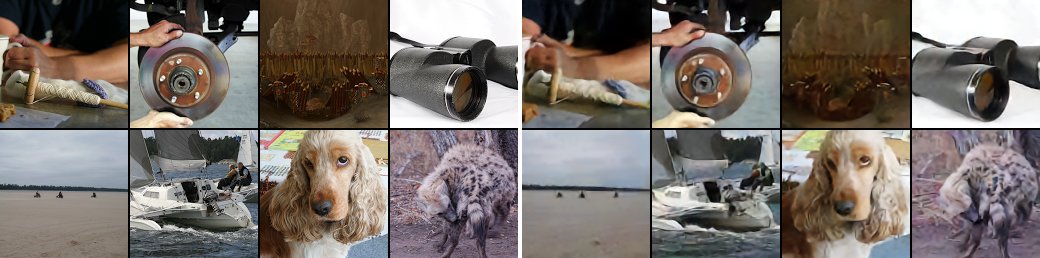
Figure 2: Left: ImageNet 128x128x3 images, right: reconstructions from a VQ-VAE with a 32x32x1 latent space, with K=512.

图 2：左：ImageNet $128\times 128\times 3$ 图像；右：潜空间为 $32\times 32\times 1$、$K=512$ 的 VQ-VAE 重建。

Reconstructions from the 32x32x1 space with discrete latents are shown in Figure 2. Even considering that we greatly reduce the dimensionality with discrete encoding, the reconstructions look only slightly blurrier than the originals. It would be possible to use a more perceptual loss function than MSE over pixels here (e.g., a GAN [12]), but we leave that as future work.

图 2 展示了 $32\times 32\times 1$ 离散潜空间的重建。即便用离散编码大幅降维，重建也只比原图略糊。此处本可用比像素 MSE 更感知的损失（例如 GAN [12]），留作未来工作。

Next, we train a PixelCNN prior on the discretised 32x32x1 latent space. As we only have 1 channel (not 3 as with colours), we only have to use spatial masking in the PixelCNN. The capacity of the PixelCNN we used was similar to those used by the authors of the PixelCNN paper [38].

接着在离散化后的 $32\times 32\times 1$ 潜空间上训练 PixelCNN 先验。因只有 1 个通道（而非彩色的 3 通道），PixelCNN 只需空间掩码。所用 PixelCNN 容量与原 PixelCNN 论文作者所用相近 [38]。

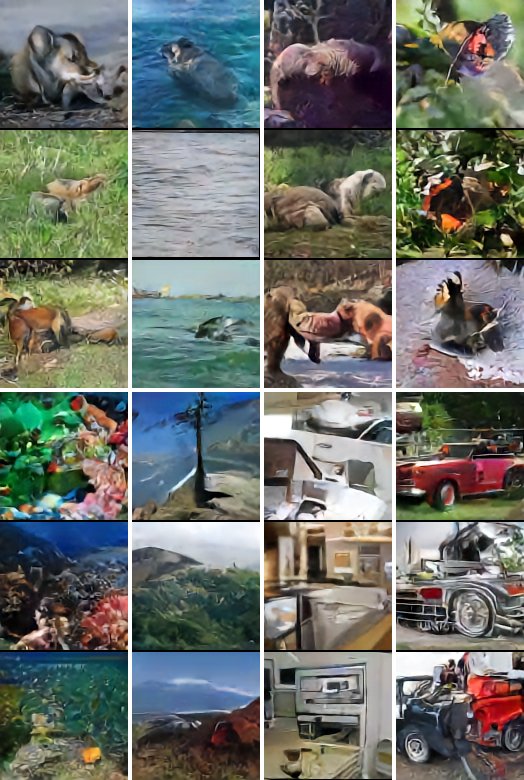
Figure 3: Samples (128x128) from a VQ-VAE with a PixelCNN prior trained on ImageNet images. From left to right: kit fox, gray whale, brown bear, admiral (butterfly), coral reef, alp, microwave, pickup.

图 3：在 ImageNet 图像上训练、配 PixelCNN 先验的 VQ-VAE 采样（$128\times 128$）。从左到右：kit fox、gray whale、brown bear、admiral（蝴蝶）、coral reef、alp、microwave、pickup。

Samples drawn from the PixelCNN were mapped to pixel-space with the decoder of the VQ-VAE and can be seen in Figure 3.

从 PixelCNN 采得的样本经 VQ-VAE 解码器映射到像素空间，见图 3。

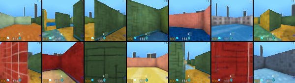
Figure 4: Samples (128x128) from a VQ-VAE with a PixelCNN prior trained on frames captured from DeepMind Lab.

图 4：在 DeepMind Lab 截帧上训练、配 PixelCNN 先验的 VQ-VAE 采样（$128\times 128$）。

We also repeat the same experiment for 84x84x3 frames drawn from the DeepMind Lab environment [2]. The reconstructions looked nearly identical to their originals. Samples drawn from the PixelCNN prior trained on the 21x21x1 latent space and decoded to the pixel space using a deconvolutional model decoder can be seen in Figure 4.

我们对来自 DeepMind Lab 环境 [2] 的 $84\times 84\times 3$ 帧重复同一实验。重建几乎与原图难辨。在 $21\times 21\times 1$ 潜空间上训练的 PixelCNN 先验采样，再用反卷积解码器映回像素空间，见图 4。

Figure 5: Top original images, Bottom: reconstructions from a 2 stage VQ-VAE, with 3 latents to model the whole image (27 bits), and as such the model cannot reconstruct the images perfectly. The reconstructions are generated by sampled from the second PixelCNN prior in the 21x21 latent domain of first VQ-VAE, and then decoded with standard VQ-VAE decoder to 84x84. A lot of the original scene, including textures, room layout and nearby walls remain, but the model does not try to store the pixel values themselves, which means the textures are generated procedurally by the PixelCNN.

图 5：上：原图；下：两阶段 VQ-VAE 的重建——仅用 3 个潜变量建模整张图（27 bit），因此无法完美重建。重建方式：在第一阶段 VQ-VAE 的 $21\times 21$ 潜域上从第二阶段 PixelCNN 先验采样，再用标准 VQ-VAE 解码器解码到 $84\times 84$。原场景的大量信息（纹理、房间布局、近墙等）得以保留，但模型并不试图存储像素值本身，故纹理由 PixelCNN 程序性生成。

Finally, we train a second VQ-VAE with a PixelCNN decoder on top of the 21x21x1 latent space from the first VQ-VAE on DM-LAB frames. This setup typically breaks VAEs as they suffer from "posterior collapse", i.e., the latents are ignored as the decoder is powerful enough to model $x$ perfectly. Our model however does not suffer from this, and the latents are meaningfully used. We use only three latent variables (each with K=512 and their own embedding space $e$) at the second stage for modelling the whole image and as such the model cannot reconstruct the image perfectly – which is consequence of compressing the image onto 3 x 9 bits, i.e. less than a float32. Reconstructions sampled from the discretised global code can be seen in Figure 5.

最后，在 DM-LAB 帧上第一阶段 VQ-VAE 的 $21\times 21\times 1$ 潜空间之上，再训练一个带 PixelCNN 解码器 的第二阶段 VQ-VAE。这种设定通常会让 VAE 陷入「后验坍塌」：解码器足够强，能完美建模 $x$，潜变量被忽略。我们的模型不受此扰，潜变量被有意义地使用。第二阶段整图仅用三个潜变量（各 $K=512$ 且有各自嵌入空间 $e$），因此无法完美重建——相当于把图像压到 $3\times 9$ bit，不到一个 float32。从图 5 可见由离散化全局码采样得到的重建。

4.3 Audio

4.3 音频

Figure 6: Left: original waveform, middle: reconstructed with same speaker-id, right: reconstructed with different speaker-id. The contents of the three waveforms are the same.

图 6：左：原始波形；中：同一说话人 id 重建；右：不同说话人 id 重建。三段波形内容相同。

In this set of experiments we evaluate the behaviour of discrete latent variables on models of raw audio. In all our audio experiments, we train a VQ-VAE that has a dilated convolutional architecture similar to WaveNet decoder. All samples for this section can be played from the following url: https://avdnoord.github.io/homepage/vqvae/.

本组实验评估离散潜变量在原始音频建模上的表现。全部音频实验中，VQ-VAE 解码器采用类似 WaveNet 的膨胀卷积结构。本节样本可在以下地址收听：https://avdnoord.github.io/homepage/vqvae/。

We first consider the VCTK dataset, which has speech recordings of 109 different speakers [41]. We train a VQ-VAE where the encoder has 6 strided convolutions with stride 2 and window-size 4. This yields a latent space 64x smaller than the original waveform. The latents consist of one feature map and the discrete space is 512-dimensional. The decoder is conditioned on both the latents and a one-hot embedding for the speaker.

首先使用含 109 位说话人录音的 VCTK 数据集 [41]。编码器含 6 个步长 2、窗口大小 4 的跨步卷积，潜空间比原波形小 64 倍；潜变量为单特征图，离散空间 512 维。解码器同时以潜变量与说话人 one-hot 嵌入为条件。

First, we ran an experiment to show that VQ-VAE can extract a latent space that only conserves long-term relevant information. After training the model, given an audio example, we can encode it to the discrete latent representation, and reconstruct by sampling from the decoder. Because the dimensionality of the discrete representation is 64 times smaller, the original sample cannot be perfectly reconstructed sample by sample. As it can be heard from the provided samples, and as shown in Figure 7, the reconstruction has the same content (same text contents), but the waveform is quite different and prosody in the voice is altered. This means that the VQ-VAE has, without any form of linguistic supervision, learned a high-level abstract space that is invariant to low-level features and only encodes the content of the speech. This experiment confirms our observations from before that important features are often those that span many dimensions in the input data space (in this case phoneme and other high-level content in waveform).

先做一个实验：说明 VQ-VAE 能抽出只保留长期相关信息的潜空间。训好后，给定音频样例，可编码到离散潜表示，再从解码器采样重建。因离散表示维数小 64 倍，无法逐采样点完美重建。从所提供样本以及图中可见：重建内容相同（同一文本内容），但波形差异明显，韵律也改变。这意味着 VQ-VAE 在无任何语言学监督的情况下，学到了一个对低级特征不变、只编码语音内容的高层抽象空间。该实验印证了前文观察：重要特征往往是那些在输入数据空间中跨越许多维度的特征（此处即波形中的音素与其他高层内容）。

We have then analysed the unconditional samples from the model to understand its capabilities. Given the compact and abstract latent representation extracted from the audio, we trained the prior on top of this representation to model the long-term dependencies in the data. For this task we have used a larger dataset of 460 speakers [30] and trained a VQ-VAE model where the resolution of discrete space is 128 times smaller. Next we trained the prior as usual on top of this representation on chunks of 40960 timesteps (2.56 seconds), which yields 320 latent timesteps. While samples drawn from even the best speech models like the original WaveNet [37] sound like babbling , samples from VQ-VAE contain clear words and part-sentences (see samples linked above). We conclude that VQ-VAE was able to model a rudimentary phoneme-level language model in a completely unsupervised fashion from raw audio waveforms.

接着分析无条件样本，以理解模型能力。在从音频抽出的紧凑抽象潜表示之上，再训练先验以建模数据中的长期依赖。该任务使用含 460 位说话人的更大数据集 [30]，训一个离散空间分辨率再小 128 倍的 VQ-VAE；先验照常在 40960 个时间步（2.56 秒）的片段上训练，对应 320 个潜时间步。即便最好的语音模型如原版 WaveNet [37]，无条件采样听起来也像咿呀学语；而 VQ-VAE 的样本含清晰单词与部分句子（见上方链接样本）。我们结论是：VQ-VAE 能在完全无监督条件下，从原始音频波形建模出初级的音素级语言模型。

Next, we attempted the speaker conversion where the latents are extracted from one speaker and then reconstructed through the decoder using a separate speaker id. As can be heard from the samples, the synthesised speech has the same content as the original sample, but with the voice from the second speaker. This experiment again demonstrates that the encoded representation has factored out speaker-specific information: the embeddings not only have the same meaning regardless of details in the waveform, but also across different voice-characteristics.

接下来尝试说话人转换：从一位说话人提取潜变量，再用另一说话人 id 经解码器重建。从样本可听出：合成语音内容与原样例相同，但声音来自第二位说话人。该实验再次说明编码表示已分解掉说话人特异信息：嵌入不仅对波形细节含义一致，跨不同嗓音特征也一致。

Finally, in an attempt to better understand the content of the discrete codes we have compared the latents one-to-one with the ground-truth phoneme-sequence (which was not used any way to train the VQ-VAE). With a 128-dimensional discrete space that runs at $25$ Hz (encoder downsampling factor of $640$), we mapped every of the 128 possible latent values to one of the 41 possible phoneme values[^1] (by taking the conditionally most likely phoneme). The accuracy of this 41-way classification was $49.3\%$, while a random latent space would result in an accuracy of $7.2\%$ (prior most likely phoneme). It is clear that these discrete latent codes obtained in a fully unsupervised way are high-level speech descriptors that are closely related to phonemes.

最后，为更好理解离散码内容，我们将潜变量与真值音素序列逐一对齐比较（音素序列未以任何方式用于训练 VQ-VAE）。在以 $25$ Hz 运行的 128 维离散空间上（编码器下采样因子 $640$），把 128 种可能潜值各自映射到 41 种可能音素之一（取条件最可能音素）。该 41 类分类准确率为 $49.3\%$，而随机潜空间约为 $7.2\%$（先验最可能音素）。可见这些完全无监督得到的离散潜码是与音素密切相关的高层语音描述子。

4.4 Video

4.4 视频

For our final experiment we have used the DeepMind Lab [2] environment to train a generative model conditioned on a given action sequence. In Figure 7 we show the initial $6$ frames that are input to the model followed by $10$ frames that are sampled from VQ-VAE with all actions set to forward (top row) and right (bottom row). Generation of the video sequence with the VQ-VAE model is done purely in the latent space, $z_{t}$ without the need to generate the actual images themselves. Each image in the sequence $x_{t}$ is then created by mapping the latents with a deterministic decoder to the pixel space after all the latents are generated using only the prior model $p(z_{1},\ldots,z_{T})$. Therefore, VQ-VAE can be used to imagine long sequences purely in latent space without resorting to pixel space. It can be seen that the model has learnt to successfully generate a sequence of frames conditioned on given action without any degradation in the visual quality whilst keeping the local geometry correct. For completeness, we trained a model without actions and obtained similar results, not shown due to space constraints.

最后一组实验用 DeepMind Lab [2] 环境，训练以给定动作序列为条件的生成模型。图 7 给出输入模型的前 $6$ 帧，随后是在全部动作为 forward（上行）与 right（下行）时从 VQ-VAE 采样的 $10$ 帧。用 VQ-VAE 生成视频序列完全在潜空间 $z_{t}$ 中进行，无需生成实际图像本身；序列中每张图 $x_{t}$ 是在仅用先验模型 $p(z_{1},\ldots,z_{T})$ 生成全部潜变量之后，再由确定性解码器映到像素空间得到的。因此 VQ-VAE 可纯在潜空间中想象长序列，而不必诉诸像素空间。可见模型已学会在给定动作条件下成功生成帧序列：视觉质量无明显退化，局部几何也保持正确。作为补充，我们也训了不带动作的模型并得到类似结果，篇幅所限未展示。

Figure 7: First 6 frames are provided to the model, following frames are generated conditioned on an action. Top: repeated action "move forward", bottom: repeated action "move right".

图 7：前 6 帧提供给模型，后续帧以动作为条件生成。上：重复动作「前进」；下：重复动作「右转」。

5 Conclusion

5 结论

In this work we have introduced VQ-VAE, a new family of models that combine VAEs with vector quantisation to obtain a discrete latent representation. We have shown that VQ-VAEs are capable of modelling very long term dependencies through their compressed discrete latent space which we have demonstrated by generating $128\times 128$ colour images, sampling action conditional video sequences and finally using audio where even an unconditional model can generate surprisingly meaningful chunks of speech and doing speaker conversion. All these experiments demonstrated that the discrete latent space learnt by VQ-VAEs capture important features of the data in a completely unsupervised manner. Moreover, VQ-VAEs achieve likelihoods that are almost as good as their continuous latent variable counterparts on CIFAR10 data. We believe that this is the first discrete latent variable model that can successfully model long range sequences and fully unsupervisedly learn high-level speech descriptors that are closely related to phonemes.

本文引入 VQ-VAE：一类把 VAE 与向量量化结合以获得离散潜表征的新模型族。我们表明 VQ-VAE 能通过压缩的离散潜空间建模很长程依赖：生成 $128\times 128$ 彩色图像、采样动作条件视频序列，以及在音频上甚至无条件模型也能生成出人意料地有意义的语音片段，并做说话人转换。这些实验都说明 VQ-VAE 学到的离散潜空间以完全无监督方式抓住了数据的重要特征。此外，在 CIFAR10 上 VQ-VAE 的似然几乎与连续潜变量对应物一样好。我们认为这是首个能成功建模长程序列、并完全无监督地学到与音素密切相关的高层语音描述子的离散潜变量模型。

References

参考文献

[1] Eirikur Agustsson, Fabian Mentzer, Michael Tschannen, Lukas Cavigelli, Radu Timofte, Luca Benini, and Luc Van Gool. Soft-to-hard vector quantization for end-to-end learned compression of images and neural networks. arXiv preprint arXiv:1704.00648 , 2017.

[2] Charles Beattie, Joel Z Leibo, Denis Teplyashin, Tom Ward, Marcus Wainwright, Heinrich Küttler, Andrew Lefrancq, Simon Green, Víctor Valdés, Amir Sadik, et al. Deepmind lab. arXiv preprint arXiv:1612.03801 , 2016.

[3] Yoshua Bengio, Nicholas Léonard, and Aaron Courville. Estimating or propagating gradients through stochastic neurons for conditional computation. arXiv preprint arXiv:1308.3432 , 2013.

[4] Samuel R Bowman, Luke Vilnis, Oriol Vinyals, Andrew M Dai, Rafal Jozefowicz, and Samy Bengio. Generating sentences from a continuous space. arXiv preprint arXiv:1511.06349 , 2015.

[5] Yuri Burda, Roger Grosse, and Ruslan Salakhutdinov. Importance weighted autoencoders. arXiv preprint arXiv:1509.00519 , 2015.

[6] Xi Chen, Yan Duan, Rein Houthooft, John Schulman, Ilya Sutskever, and Pieter Abbeel. Infogan: Interpretable representation learning by information maximizing generative adversarial nets. CoRR , abs/1606.03657, 2016.

[7] Xi Chen, Diederik P Kingma, Tim Salimans, Yan Duan, Prafulla Dhariwal, John Schulman, Ilya Sutskever, and Pieter Abbeel. Variational lossy autoencoder. arXiv preprint arXiv:1611.02731 , 2016.

[8] Aaron Courville, James Bergstra, and Yoshua Bengio. A spike and slab restricted boltzmann machine. In Proceedings of the Fourteenth International Conference on Artificial Intelligence and Statistics , pages 233–241, 2011.

[9] Emily Denton, Sam Gross, and Rob Fergus. Semi-supervised learning with context-conditional generative adversarial networks. arXiv preprint arXiv:1611.06430 , 2016.

[10] Laurent Dinh, Jascha Sohl-Dickstein, and Samy Bengio. Density estimation using real nvp. arXiv preprint arXiv:1605.08803 , 2016.

[11] Chelsea Finn, Ian Goodfellow, and Sergey Levine. Unsupervised learning for physical interaction through video prediction. In Advances in Neural Information Processing Systems , pages 64–72, 2016.

[12] Ian Goodfellow, Jean Pouget-Abadie, Mehdi Mirza, Bing Xu, David Warde-Farley, Sherjil Ozair, Aaron Courville, and Yoshua Bengio. Generative adversarial nets. In Advances in neural information processing systems , pages 2672–2680, 2014.

[13] Karol Gregor, Frederic Besse, Danilo Jimenez Rezende, Ivo Danihelka, and Daan Wierstra. Towards conceptual compression. In Advances In Neural Information Processing Systems , pages 3549–3557, 2016.

[14] Karol Gregor, Ivo Danihelka, Andriy Mnih, Charles Blundell, and Daan Wierstra. Deep autoregressive networks. arXiv preprint arXiv:1310.8499 , 2013.

[15] Ishaan Gulrajani, Kundan Kumar, Faruk Ahmed, Adrien Ali Taiga, Francesco Visin, David Vázquez, and Aaron C. Courville. Pixelvae: A latent variable model for natural images. CoRR , abs/1611.05013, 2016.

[16] Geoffrey E Hinton and Ruslan R Salakhutdinov. Reducing the dimensionality of data with neural networks. science , 313(5786):504–507, 2006.

[17] Judy Hoffman, Erik Rodner, Jeff Donahue, Trevor Darrell, and Kate Saenko. Efficient learning of domain-invariant image representations. arXiv preprint arXiv:1301.3224 , 2013.

[18] Phillip Isola, Jun-Yan Zhu, Tinghui Zhou, and Alexei A Efros. Image-to-image translation with conditional adversarial networks. arXiv preprint arXiv:1611.07004 , 2016.

[19] Eric Jang, Shixiang Gu, and Ben Poole. Categorical reparameterization with gumbel-softmax. arXiv preprint arXiv:1611.01144 , 2016.

[20] Nal Kalchbrenner, Aaron van den Oord, Karen Simonyan, Ivo Danihelka, Oriol Vinyals, Alex Graves, and Koray Kavukcuoglu. Video pixel networks. arXiv preprint arXiv:1610.00527 , 2016.

[21] Diederik Kingma and Jimmy Ba. Adam: A method for stochastic optimization. arXiv preprint arXiv:1412.6980 , 2014.

[22] Diederik P Kingma, Tim Salimans, Rafal Jozefowicz, Xi Chen, Ilya Sutskever, and Max Welling. Improved variational inference with inverse autoregressive flow. NIPS 2016 , 2016.

[23] Diederik P Kingma and Max Welling. Auto-encoding variational bayes. arXiv preprint arXiv:1312.6114 , 2013.

[24] Christian Ledig, Lucas Theis, Ferenc Huszár, Jose Caballero, Andrew Cunningham, Alejandro Acosta, Andrew Aitken, Alykhan Tejani, Johannes Totz, Zehan Wang, et al. Photo-realistic single image super-resolution using a generative adversarial network. arXiv preprint arXiv:1609.04802 , 2016.

[25] Chris J Maddison, Andriy Mnih, and Yee Whye Teh. The concrete distribution: A continuous relaxation of discrete random variables. arXiv preprint arXiv:1611.00712 , 2016.

[26] Soroush Mehri, Kundan Kumar, Ishaan Gulrajani, Rithesh Kumar, Shubham Jain, Jose Sotelo, Aaron Courville, and Yoshua Bengio. Samplernn: An unconditional end-to-end neural audio generation model. arXiv preprint arXiv:1612.07837 , 2016.

[27] Andriy Mnih and Karol Gregor. Neural variational inference and learning in belief networks. arXiv preprint arXiv:1402.0030 , 2014.

[28] Andriy Mnih and Danilo Jimenez Rezende. Variational inference for monte carlo objectives. CoRR , abs/1602.06725, 2016.

[29] Aaron van den Oord, Nal Kalchbrenner, and Koray Kavukcuoglu. Pixel recurrent neural networks. arXiv preprint arXiv:1601.06759 , 2016.

[30] Vassil Panayotov, Guoguo Chen, Daniel Povey, and Sanjeev Khudanpur. Librispeech: an asr corpus based on public domain audio books. In Acoustics, Speech and Signal Processing (ICASSP), 2015 IEEE International Conference on , pages 5206–5210. IEEE, 2015.

[31] Danilo Jimenez Rezende and Shakir Mohamed. Variational inference with normalizing flows. arXiv preprint arXiv:1505.05770 , 2015.

[32] Danilo Jimenez Rezende, Shakir Mohamed, and Daan Wierstra. Stochastic backpropagation and approximate inference in deep generative models. arXiv preprint arXiv:1401.4082 , 2014.

[33] Ruslan Salakhutdinov and Geoffrey Hinton. Deep boltzmann machines. In Artificial Intelligence and Statistics , pages 448–455, 2009.

[34] Adam Santoro, Sergey Bartunov, Matthew Botvinick, Daan Wierstra, and Timothy Lillicrap. One-shot learning with memory-augmented neural networks. arXiv preprint arXiv:1605.06065 , 2016.

[35] Richard S Sutton and Andrew G Barto. Reinforcement learning: An introduction , volume 1. MIT press Cambridge, 1998.

[36] Lucas Theis, Wenzhe Shi, Andrew Cunningham, and Ferenc Huszár. Lossy image compression with compressive autoencoders. arXiv preprint arXiv:1703.00395 , 2017.

[37] Aäron van den Oord, Sander Dieleman, Heiga Zen, Karen Simonyan, Oriol Vinyals, Alex Graves, Nal Kalchbrenner, Andrew Senior, and Koray Kavukcuoglu. Wavenet: A generative model for raw audio. CoRR abs/1609.03499 , 2016.

[38] Aaron van den Oord, Nal Kalchbrenner, Lasse Espeholt, Oriol Vinyals, Alex Graves, et al. Conditional image generation with pixelcnn decoders. In Advances in Neural Information Processing Systems , pages 4790–4798, 2016.

[39] Pascal Vincent, Hugo Larochelle, Isabelle Lajoie, Yoshua Bengio, and Pierre-Antoine Manzagol. Stacked denoising autoencoders: Learning useful representations in a deep network with a local denoising criterion. Journal of Machine Learning Research , 11(Dec):3371–3408, 2010.

[40] Oriol Vinyals, Alexander Toshev, Samy Bengio, and Dumitru Erhan. Show and tell: A neural image caption generator. In Proceedings of the IEEE Conference on Computer Vision and Pattern Recognition , pages 3156–3164, 2015.

[41] Junichi Yamagishi. English multi-speaker corpus for cstr voice cloning toolkit. URL http://homepages. inf. ed. ac. uk/jyamagis/page3/page58/page58. html , 2012.

[42] Zichao Yang, Zhiting Hu, Ruslan Salakhutdinov, and Taylor Berg-Kirkpatrick. Improved variational autoencoders for text modeling using dilated convolutions. CoRR , abs/1702.08139, 2017.

Appendix A Appendix

附录 A 附录

A.1 VQ-VAE dictionary updates with Exponential Moving Averages

A.1 用指数滑动平均更新 VQ-VAE 字典

As mentioned in Section 3.2, one can also use exponential moving averages (EMA) to update the dictionary items instead of the loss term from Equation 3:

如第 3.2 节所述，也可用指数滑动平均（EMA）更新字典项，以替代式 (3) 中的损失项：

$$\|\text{sg}[z_{e}(x)]-e\|^{2}_{2}. \tag{4}$$

Let $\{z_{i,1},z_{i,2},\dots,z_{i,n_{i}}\}$ be the set of $n_{i}$ outputs from the encoder that are closest to dictionary item $e_{i}$, so that we can write the loss as:

令 $\{z_{i,1},z_{i,2},\dots,z_{i,n_{i}}\}$ 为编码器输出中最接近字典项 $e_{i}$ 的 $n_{i}$ 个输出所成集合，则损失可写为：

$$\sum_{j}^{n_{i}}\|z_{i,j}-e_{i}\|^{2}_{2}. \tag{5}$$

The optimal value for $e_{i}$ has a closed form solution, which is simply the average of elements in the set:

$e_{i}$ 的最优值有闭式解，即该集合中元素的平均：

$$e_{i}=\frac{1}{n_{i}}\sum_{j}^{n_{i}}z_{i,j}.$$

This update is typically used in algorithms such as K-Means.

这类更新常见于 K-Means 等算法。

However, we cannot use this update directly when working with minibatches. Instead we can use exponential moving averages as an online version of this update:

但在小批量设定下不能直接用该更新。可改用指数滑动平均作为该更新的在线版本：

$$\displaystyle N^{(t)}_{i} \\ \displaystyle:=N^{(t-1)}_{i}*\gamma+n^{(t)}_{i}(1-\gamma) \\ \displaystyle m^{(t)}_{i} \\ \displaystyle:=m^{(t-1)}_{i}*\gamma+\sum_{j}z^{(t)}_{i,j}(1-\gamma) \\ \displaystyle e^{(t)}_{i} \\ \displaystyle:=\frac{m^{(t)}_{i}}{N^{(t)}_{i}}, \tag{6}$$

with $\gamma$ a value between 0 and 1. We found $\gamma=0.99$ to work well in practice.

其中 $\gamma$ 取值于 0 与 1 之间。实践中发现 $\gamma=0.99$ 效果良好。