VoxelNet: End-to-End Learning for Point Cloud Based 3D Object Detection

VoxelNet：面向点云三维目标检测的端到端学习

Yin Zhou Affiliation:  Apple Inc Email:  yzhou3@apple.com    Oncel Tuzel Affiliation:  Apple Inc Email:  otuzel@apple.com

Abstract

摘要

Accurate detection of objects in 3D point clouds is a central problem in many applications, such as autonomous navigation, housekeeping robots, and augmented/virtual reality. To interface a highly sparse LiDAR point cloud with a region proposal network (RPN), most existing efforts have focused on hand-crafted feature representations, for example, a bird’s eye view projection. In this work, we remove the need of manual feature engineering for 3D point clouds and propose VoxelNet, a generic 3D detection network that unifies feature extraction and bounding box prediction into a single stage, end-to-end trainable deep network. Specifically, VoxelNet divides a point cloud into equally spaced 3D voxels and transforms a group of points within each voxel into a unified feature representation through the newly introduced voxel feature encoding (VFE) layer. In this way, the point cloud is encoded as a descriptive volumetric representation, which is then connected to a RPN to generate detections. Experiments on the KITTI car detection benchmark show that VoxelNet outperforms the state-of-the-art LiDAR based 3D detection methods by a large margin. Furthermore, our network learns an effective discriminative representation of objects with various geometries, leading to encouraging results in 3D detection of pedestrians and cyclists, based on only LiDAR.

在三维点云里准确检出物体，是自动驾驶、家用机器人和增强／虚拟现实等许多应用的核心问题。要把高度稀疏的激光雷达点云接到区域提议网络（RPN）上，以往工作大多依赖手工特征，例如鸟瞰投影。本文去掉对三维点云的人工特征工程，提出 VoxelNet：把特征提取和边界框预测收进同一阶段、可端到端训练的通用三维检测网络。具体做法是把点云划成等间距的三维体素，再用新引入的体素特征编码（VFE）层，把每个体素内的一组点变成统一的特征表示。点云由此被编码成有描述力的体表示，再接到 RPN 上产生检测结果。在 KITTI 车辆检测基准上，VoxelNet 大幅超过当时最强的纯激光雷达三维检测方法。网络还能学到对不同几何形状有判别力的表示，仅凭激光雷达，在行人和骑行者的三维检测上也得到了可观结果。

1 Introduction

1 引言

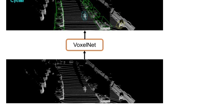
Figure 1: VoxelNet directly operates on the raw point cloud (no need for feature engineering) and produces the 3D detection results using a single end-to-end trainable network.

图 1：VoxelNet 直接处理原始点云（无需特征工程），用单一可端到端训练的网络给出三维检测结果。

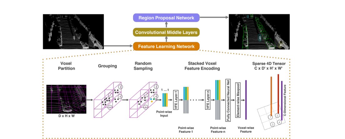
Figure 2: VoxelNet architecture. The feature learning network takes a raw point cloud as input, partitions the space into voxels, and transforms points within each voxel to a vector representation characterizing the shape information. The space is represented as a sparse 4D tensor. The convolutional middle layers processes the 4D tensor to aggregate spatial context. Finally, a RPN generates the 3D detection.

图 2：VoxelNet 架构。特征学习网络接收原始点云，把空间划成体素，再把每个体素内的点变成刻画形状信息的向量。空间被表示成稀疏四维张量。卷积中间层处理该四维张量以汇聚空间上下文。最后由 RPN 产生三维检测。

Point cloud based 3D object detection is an important component of a variety of real-world applications, such as autonomous navigation [11, 14], housekeeping robots [26], and augmented/virtual reality [27]. Compared to image-based detection, LiDAR provides reliable depth information that can be used to accurately localize objects and characterize their shapes [21, 5]. However, unlike images, LiDAR point clouds are sparse and have highly variable point density, due to factors such as non-uniform sampling of the 3D space, effective range of the sensors, occlusion, and the relative pose. To handle these challenges, many approaches manually crafted feature representations for point clouds that are tuned for 3D object detection. Several methods project point clouds into a perspective view and apply image-based feature extraction techniques [28, 15, 22]. Other approaches rasterize point clouds into a 3D voxel grid and encode each voxel with hand-crafted features [41, 9, 37, 38, 21, 5]. However, these manual design choices introduce an information bottleneck that prevents these approaches from effectively exploiting 3D shape information and the required invariances for the detection task. A major breakthrough in recognition [20] and detection [13] tasks on images was due to moving from hand-crafted features to machine-learned features.

基于点云的三维目标检测，是自动驾驶[11, 14]、家用机器人[26]和增强／虚拟现实[27]等许多实际应用的重要组成部分。与基于图像的检测相比，激光雷达能提供可靠的深度信息，用来精确定位物体并刻画其形状[21, 5]。但和图像不同，激光雷达点云稀疏，点密度变化很大，原因包括三维空间的非均匀采样、传感器有效距离、遮挡以及相对位姿。为应对这些困难，许多方法为点云手工设计了面向三维检测的特征。有的把点云投到透视视图，再套用基于图像的特征提取[28, 15, 22]；有的把点云栅格化成三维体素网格，再用手工特征编码每个体素[41, 9, 37, 38, 21, 5]。这些人工选择会造成信息瓶颈，让模型难以有效利用三维形状信息，也难以学到检测任务所需的不变性。图像识别[20]和检测[13]后来能取得突破，关键一步正是从手工特征转向机器学到的特征。

Recently, Qi et al.[29] proposed PointNet, an end-to-end deep neural network that learns point-wise features directly from point clouds. This approach demonstrated impressive results on 3D object recognition, 3D object part segmentation, and point-wise semantic segmentation tasks. In [30], an improved version of PointNet was introduced which enabled the network to learn local structures at different scales. To achieve satisfactory results, these two approaches trained feature transformer networks on all input points ($\sim$1k points). Since typical point clouds obtained using LiDARs contain $\sim$100k points, training the architectures as in [29, 30] results in high computational and memory requirements. Scaling up 3D feature learning networks to orders of magnitude more points and to 3D detection tasks are the main challenges that we address in this paper.

最近，Qi 等人[29]提出 PointNet，这是一个直接从点云学习逐点特征的端到端深度网络，在三维物体识别、部件分割和逐点语义分割上表现突出。随后[30]给出了改进版，使网络能在不同尺度上学习局部结构。这两项工作要对全部输入点（约一千个点）训练特征变换网络；而典型激光雷达点云约有十万个点，若直接套用[29, 30]的结构，计算和显存开销都会很高。如何把三维特征学习网络扩展到高出几个数量级的点数，并用于三维检测，正是本文要解决的主要挑战。

Region proposal network (RPN) [32] is a highly optimized algorithm for efficient object detection [17, 5, 31, 24]. However, this approach requires data to be dense and organized in a tensor structure (e.g. image, video) which is not the case for typical LiDAR point clouds. In this paper, we close the gap between point set feature learning and RPN for 3D detection task.

区域提议网络（RPN）[32]是高效目标检测里高度优化的算法[17, 5, 31, 24]。不过它要求数据密集，并组织成张量结构（例如图像、视频），典型激光雷达点云并不满足这一条件。本文要弥补点集特征学习与三维检测所用 RPN 之间的这一缺口。

We present VoxelNet, a generic 3D detection framework that simultaneously learns a discriminative feature representation from point clouds and predicts accurate 3D bounding boxes, in an end-to-end fashion, as shown in Figure 2. We design a novel voxel feature encoding (VFE) layer, which enables inter-point interaction within a voxel, by combining point-wise features with a locally aggregated feature. Stacking multiple VFE layers allows learning complex features for characterizing local 3D shape information. Specifically, VoxelNet divides the point cloud into equally spaced 3D voxels, encodes each voxel via stacked VFE layers, and then 3D convolution further aggregates local voxel features, transforming the point cloud into a high-dimensional volumetric representation. Finally, a RPN consumes the volumetric representation and yields the detection result. This efficient algorithm benefits both from the sparse point structure and efficient parallel processing on the voxel grid.

我们提出 VoxelNet，这是一个通用的三维检测框架，能同时从点云学习有判别力的特征表示，并以端到端的方式预测准确的三维边界框，如图 2 所示。我们设计了体素特征编码（VFE）层：它把逐点特征与局部汇聚特征结合，使体素内的点能够相互作用。堆叠多层 VFE，就能学到刻画局部三维形状的复杂特征。具体而言，VoxelNet 把点云划成等间距三维体素，用堆叠的 VFE 层编码每个体素，再用三维卷积进一步汇聚局部体素特征，从而把点云变成高维体表示。最后由 RPN 消费这一体表示并给出检测结果。这一算法既利用了点的稀疏结构，也能在体素网格上高效并行计算。

We evaluate VoxelNet on the bird’s eye view detection and the full 3D detection tasks, provided by the KITTI benchmark [11]. Experimental results show that VoxelNet outperforms the state-of-the-art LiDAR based 3D detection methods by a large margin. We also demonstrate that VoxelNet achieves highly encouraging results in detecting pedestrians and cyclists from LiDAR point cloud.

我们在 KITTI 基准[11]提供的鸟瞰检测和完整三维检测任务上评估 VoxelNet。实验表明，它大幅超过当时最强的纯激光雷达三维检测方法。我们也展示了 VoxelNet 仅凭激光雷达点云检测行人和骑行者时，同样能得到相当积极的结果。

1.1 Related Work

1.1 相关工作

Rapid development of 3D sensor technology has motivated researchers to develop efficient representations to detect and localize objects in point clouds. Some of the earlier methods for feature representation are [39, 8, 7, 19, 40, 33, 6, 25, 1, 34, 2]. These hand-crafted features yield satisfactory results when rich and detailed 3D shape information is available. However their inability to adapt to more complex shapes and scenes, and learn required invariances from data resulted in limited success for uncontrolled scenarios such as autonomous navigation.

三维传感器技术的快速发展，推动研究者去设计能在点云中检测并定位物体的高效表示。较早的特征表示工作包括[39, 8, 7, 19, 40, 33, 6, 25, 1, 34, 2]。当三维形状信息丰富而细致时，这些手工特征可以给出不错的结果。但它们难以适应更复杂的形状与场景，也无法从数据中学到所需的不变性，因此在自动驾驶这类不受控场景里效果有限。

Given that images provide detailed texture information, many algorithms infered the 3D bounding boxes from 2D images [4, 3, 42, 43, 44, 36]. However, the accuracy of image-based 3D detection approaches are bounded by the accuracy of the depth estimation.

图像能提供细致的纹理信息，因此不少算法从二维图像推断三维边界框[4, 3, 42, 43, 44, 36]。不过，基于图像的三维检测精度受深度估计精度的限制。

Several LIDAR based 3D object detection techniques utilize a voxel grid representation. [41, 9] encode each nonempty voxel with 6 statistical quantities that are derived from all the points contained within the voxel. [37] fuses multiple local statistics to represent each voxel. [38] computes the truncated signed distance on the voxel grid. [21] uses binary encoding for the 3D voxel grid. [5] introduces a multi-view representation for a LiDAR point cloud by computing a multi-channel feature map in the bird’s eye view and the cylindral coordinates in the frontal view. Several other studies project point clouds onto a perspective view and then use image-based feature encoding schemes [28, 15, 22].

若干基于激光雷达的三维目标检测方法采用体素网格表示。[41, 9]用体素内全部点导出的 6 个统计量来编码每个非空体素。[37]融合多种局部统计来表示每个体素。[38]在体素网格上计算截断符号距离。[21]对三维体素网格做二值编码。[5]为激光雷达点云引入多视图表示，在鸟瞰视图中计算多通道特征图，并在前视中使用柱面坐标。还有研究把点云投到透视视图，再使用基于图像的特征编码方案[28, 15, 22]。

There are also several multi-modal fusion methods that combine images and LiDAR to improve detection accuracy [10, 16, 5]. These methods provide improved performance compared to LiDAR-only 3D detection, particularly for small objects (pedestrians, cyclists) or when the objects are far, since cameras provide an order of magnitude more measurements than LiDAR. However the need for an additional camera that is time synchronized and calibrated with the LiDAR restricts their use and makes the solution more sensitive to sensor failure modes. In this work we focus on LiDAR-only detection.

也有若干多模态融合方法把图像和激光雷达结合起来以提高检测精度[10, 16, 5]。与只用激光雷达的三维检测相比，这些方法往往更好，尤其是对小物体（行人、骑行者）或远处物体，因为相机的测量数量通常比激光雷达高一个数量级。不过，这需要一台与激光雷达时间同步并标定好的额外相机，使用场景更受限，也对传感器故障更敏感。本文只关注纯激光雷达检测。

1.2 Contributions

1.2 本文贡献

• • We propose a novel end-to-end trainable deep architecture for point-cloud-based 3D detection, VoxelNet, that directly operates on sparse 3D points and avoids information bottlenecks introduced by manual feature engineering.

• 我们提出面向点云三维检测的新型可端到端训练深度架构 VoxelNet，它直接处理稀疏三维点，避开手工特征工程带来的信息瓶颈。

• • We present an efficient method to implement VoxelNet which benefits both from the sparse point structure and efficient parallel processing on the voxel grid.

• 我们给出一种高效实现 VoxelNet 的方法，既能利用点云的稀疏结构，又能在体素网格上并行计算。

• • We conduct experiments on KITTI benchmark and show that VoxelNet produces state-of-the-art results in LiDAR-based car, pedestrian, and cyclist detection benchmarks.

• 我们在 KITTI 基准上做实验，表明 VoxelNet 在基于激光雷达的车辆、行人和骑行者检测上都达到了当时的领先水平。

2 VoxelNet

In this section we explain the architecture of VoxelNet, the loss function used for training, and an efficient algorithm to implement the network.

本节说明 VoxelNet 的网络结构、训练所用的损失函数，以及一种高效的实现算法。

2.1 VoxelNet Architecture

2.1 VoxelNet 架构

The proposed VoxelNet consists of three functional blocks: (1) Feature learning network, (2) Convolutional middle layers, and (3) Region proposal network [32], as illustrated in Figure 2. We provide a detailed introduction of VoxelNet in the following sections.

VoxelNet 由三个功能模块组成：（1）特征学习网络，（2）卷积中间层，以及（3）区域提议网络[32]，如图 2 所示。下面各小节给出详细介绍。

2.1.1 Feature Learning Network

Voxel Partition Given a point cloud, we subdivide the 3D space into equally spaced voxels as shown in Figure 2. Suppose the point cloud encompasses 3D space with range $D$, $H$, $W$ along the Z, Y, X axes respectively. We define each voxel of size $v_{D}$, $v_{H}$, and $v_{W}$ accordingly. The resulting 3D voxel grid is of size $D^{\prime}=D/v_{D},H^{\prime}=H/v_{H},W^{\prime}=W/v_{W}$. Here, for simplicity, we assume $D$, $H$, $W$ are a multiple of $v_{D}$, $v_{H}$, $v_{W}$.

2.1.1 特征学习网络

体素划分 给定点云，我们把三维空间划成等间距体素，如图 2 所示。设点云沿 Z、Y、X 轴覆盖的范围分别为 $D$、$H$、$W$，相应定义体素尺寸 $v_{D}$、$v_{H}$ 和 $v_{W}$。得到的三维体素网格大小为 $D^{\prime}=D/v_{D},H^{\prime}=H/v_{H},W^{\prime}=W/v_{W}$。为表述简便，这里假定 $D$、$H$、$W$ 分别是 $v_{D}$、$v_{H}$、$v_{W}$ 的整数倍。

Grouping We group the points according to the voxel they reside in. Due to factors such as distance, occlusion, object’s relative pose, and non-uniform sampling, the LiDAR point cloud is sparse and has highly variable point density throughout the space. Therefore, after grouping, a voxel will contain a variable number of points. An illustration is shown in Figure 2, where Voxel-1 has significantly more points than Voxel-2 and Voxel-4, while Voxel-3 contains no point.

分组 我们按点所在的体素把点分组。由于距离、遮挡、物体相对位姿和非均匀采样等因素，激光雷达点云稀疏，空间各处的点密度差异很大。因此分组之后，每个体素里的点数并不固定。图 2 给出示意：体素 1 的点数明显多于体素 2 和体素 4，而体素 3 里没有点。

Random Sampling Typically a high-definition LiDAR point cloud is composed of $\sim$100k points. Directly processing all the points not only imposes increased memory/efficiency burdens on the computing platform, but also highly variable point density throughout the space might bias the detection. To this end, we randomly sample a fixed number, $T$, of points from those voxels containing more than $T$ points. This sampling strategy has two purposes, (1) computational savings (see Section 2.3 for details); and (2) decreases the imbalance of points between the voxels which reduces the sampling bias, and adds more variation to training.

随机采样 高清激光雷达点云通常约有十万个点。直接处理全部点会加重计算平台的显存和效率负担，而且空间中点密度的剧烈变化也可能给检测带来偏差。为此，我们对点数超过 $T$ 的体素，从中随机采样固定数量 $T$ 个点。这一策略有两个目的：（1）节省计算（详见第 2.3 节）；（2）减轻体素之间的点数不均衡，从而降低采样偏差，并为训练增加更多变化。

Stacked Voxel Feature Encoding The key innovation is the chain of VFE layers. For simplicity, Figure 2 illustrates the hierarchical feature encoding process for one voxel. Without loss of generality, we use VFE Layer-1 to describe the details in the following paragraph. Figure 3 shows the architecture for VFE Layer-1.

堆叠的体素特征编码 关键创新是一串相接的 VFE 层。为简明起见，图 2 只画出一个体素上的层次化特征编码过程。不失一般性，下面用 VFE 第 1 层来说明细节。图 3 给出了 VFE 第 1 层的结构。

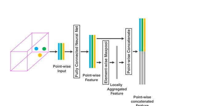
Figure 3: Voxel feature encoding layer.

图 3：体素特征编码层。

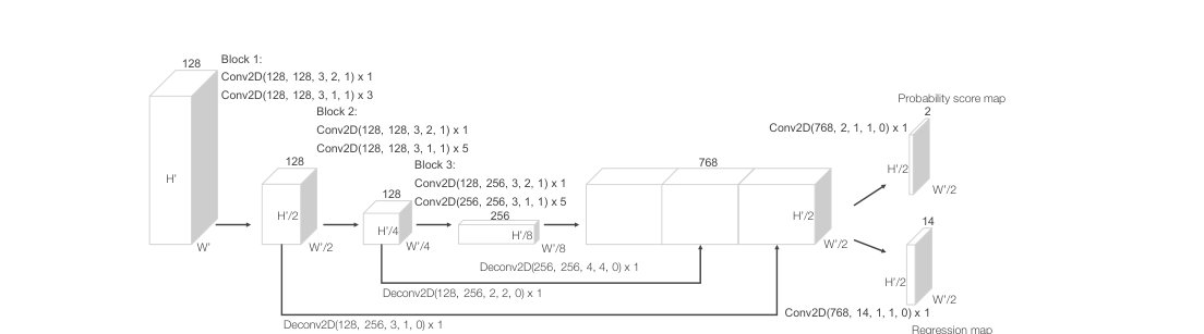
Figure 4: Region proposal network architecture.

图 4：区域提议网络架构。

Denote $\mathbf{V}=\{\mathbf{p}_{i}=[x_{i},y_{i},z_{i},r_{i}]^{T}\in\mathbb{R}^{4}\}_{i=1\ldots t}$ as a non-empty voxel containing $t\leq T$ LiDAR points, where $\mathbf{p}_{i}$ contains XYZ coordinates for the $i$-th point and $r_{i}$ is the received reflectance. We first compute the local mean as the centroid of all the points in $\mathbf{V}$, denoted as $(v_{x},v_{y},v_{z})$. Then we augment each point $\mathbf{p}_{i}$ with the relative offset w.r.t. the centroid and obtain the input feature set $\mathbf{V}_{\textrm{in}}=\{\hat{\mathbf{p}}_{i}=[x_{i},y_{i},z_{i},r_{i},x_{i}-v_{x},y_{i}-v_{y},z_{i}-v_{z}]^{T}\in\mathbb{R}^{7}\}_{i=1\ldots t}$. Next, each $\hat{\mathbf{p}}_{i}$ is transformed through the fully connected network (FCN) into a feature space, where we can aggregate information from the point features $\mathbf{f}_{i}\in\mathbb{R}^{m}$ to encode the shape of the surface contained within the voxel. The FCN is composed of a linear layer, a batch normalization (BN) layer, and a rectified linear unit (ReLU) layer. After obtaining point-wise feature representations, we use element-wise MaxPooling across all $\mathbf{f}_{i}$ associated to $\mathbf{V}$ to get the locally aggregated feature $\tilde{\mathbf{f}}\in\mathbb{R}^{m}$ for $\mathbf{V}$. Finally, we augment each $\mathbf{f}_{i}$ with $\tilde{\mathbf{f}}$ to form the point-wise concatenated feature as $\mathbf{f}_{i}^{out}=[\mathbf{f}_{i}^{T},\tilde{\mathbf{f}}^{T}]^{T}\in\mathbb{R}^{2m}$. Thus we obtain the output feature set $\mathbf{V}_{\textrm{out}}=\{\mathbf{f}_{i}^{out}\}_{i\ldots t}$. All non-empty voxels are encoded in the same way and they share the same set of parameters in FCN.

记非空体素 $\mathbf{V}=\{\mathbf{p}_{i}=[x_{i},y_{i},z_{i},r_{i}]^{T}\in\mathbb{R}^{4}\}_{i=1\ldots t}$ 含有 $t\leq T$ 个激光雷达点，其中 $\mathbf{p}_{i}$ 是第 $i$ 个点的 XYZ 坐标，$r_{i}$ 是接收到的反射率。我们先计算体素内所有点的局部均值作为质心，记为 $(v_{x},v_{y},v_{z})$。然后用相对于质心的偏移扩充每个点 $\mathbf{p}_{i}$，得到输入特征集合 $\mathbf{V}_{\textrm{in}}=\{\hat{\mathbf{p}}_{i}=[x_{i},y_{i},z_{i},r_{i},x_{i}-v_{x},y_{i}-v_{y},z_{i}-v_{z}]^{T}\in\mathbb{R}^{7}\}_{i=1\ldots t}$。接着，每个 $\hat{\mathbf{p}}_{i}$ 经全连接网络（FCN）变换到特征空间，我们再从点特征 $\mathbf{f}_{i}\in\mathbb{R}^{m}$ 中汇聚信息，以编码体素内表面的形状。FCN 由线性层、批归一化（BN）层和整流线性单元（ReLU）层组成。得到逐点特征后，对属于 $\mathbf{V}$ 的全部 $\mathbf{f}_{i}$ 做逐元素 MaxPooling，得到该体素的局部汇聚特征 $\tilde{\mathbf{f}}\in\mathbb{R}^{m}$。最后把每个 $\mathbf{f}_{i}$ 与 $\tilde{\mathbf{f}}$ 拼接，形成逐点拼接特征 $\mathbf{f}_{i}^{out}=[\mathbf{f}_{i}^{T},\tilde{\mathbf{f}}^{T}]^{T}\in\mathbb{R}^{2m}$。于是输出特征集合为 $\mathbf{V}_{\textrm{out}}=\{\mathbf{f}_{i}^{out}\}_{i\ldots t}$。所有非空体素都以同一方式编码，并共享同一套 FCN 参数。

We use $\textrm{VFE-i}(c_{in},c_{out})$ to represent the $i$-th VFE layer that transforms input features of dimension $c_{in}$ into output features of dimension $c_{out}$. The linear layer learns a matrix of size $c_{in}\times(c_{out}/2)$, and the point-wise concatenation yields the output of dimension $c_{out}$.

我们用 $\textrm{VFE-i}(c_{in},c_{out})$ 表示第 $i$ 个 VFE 层，它把维度为 $c_{in}$ 的输入特征变换成维度为 $c_{out}$ 的输出特征。线性层学习大小为 $c_{in}\times(c_{out}/2)$ 的矩阵，逐点拼接后得到维度为 $c_{out}$ 的输出。

Because the output feature combines both point-wise features and locally aggregated feature, stacking VFE layers encodes point interactions within a voxel and enables the final feature representation to learn descriptive shape information. The voxel-wise feature is obtained by transforming the output of VFE-$n$ into $\mathbb{R}^{C}$ via FCN and applying element-wise Maxpool where $C$ is the dimension of the voxel-wise feature, as shown in Figure 2.

由于输出特征同时包含逐点特征和局部汇聚特征，堆叠 VFE 层就能编码体素内点与点的相互作用，使最终表示学到有描述力的形状信息。体素级特征则是把 VFE-$n$ 的输出经 FCN 变换到 $\mathbb{R}^{C}$，再做逐元素 Maxpool 得到，其中 $C$ 是体素级特征的维度，如图 2 所示。

Sparse Tensor Representation By processing only the non-empty voxels, we obtain a list of voxel features, each uniquely associated to the spatial coordinates of a particular non-empty voxel. The obtained list of voxel-wise features can be represented as a sparse 4D tensor, of size $C\times D^{\prime}\times H^{\prime}\times W^{\prime}$ as shown in Figure 2. Although the point cloud contains $\sim$100k points, more than $90\%$ of voxels typically are empty. Representing non-empty voxel features as a sparse tensor greatly reduces the memory usage and computation cost during backpropagation, and it is a critical step in our efficient implementation.

稀疏张量表示 只处理非空体素，我们得到一份体素特征列表，每一项都唯一对应某个非空体素的空间坐标。这份体素级特征可以写成大小为 $C\times D^{\prime}\times H^{\prime}\times W^{\prime}$ 的稀疏四维张量，如图 2 所示。尽管点云约有十万个点，通常超过 90% 的体素是空的。把非空体素特征表示成稀疏张量，能在反向传播时大幅降低显存和计算开销，也是我们高效实现里的关键一步。

2.1.2 Convolutional Middle Layers

We use $\textrm{Conv}M\textrm{D}(c_{in},c_{out},\mathbf{k},\mathbf{s},\mathbf{p})$ to represent an $M$-dimensional convolution operator where $c_{in}$ and $c_{out}$ are the number of input and output channels, $\mathbf{k}$, $\mathbf{s}$, and $\mathbf{p}$ are the $M$-dimensional vectors corresponding to kernel size, stride size and padding size respectively. When the size across the $M$-dimensions are the same, we use a scalar to represent the size e.g. $k$ for $\mathbf{k}=(k,k,k)$.

2.1.2 卷积中间层

我们用 $\textrm{Conv}M\textrm{D}(c_{in},c_{out},\mathbf{k},\mathbf{s},\mathbf{p})$ 表示 $M$ 维卷积算子，其中 $c_{in}$ 和 $c_{out}$ 是输入、输出通道数，$\mathbf{k}$、$\mathbf{s}$ 和 $\mathbf{p}$ 分别是对应卷积核大小、步长和填充的 $M$ 维向量。当 $M$ 个维度上的尺寸相同时，我们用标量表示，例如用 $k$ 表示 $\mathbf{k}=(k,k,k)$。

Each convolutional middle layer applies 3D convolution, BN layer, and ReLU layer sequentially. The convolutional middle layers aggregate voxel-wise features within a progressively expanding receptive field, adding more context to the shape description. The detailed sizes of the filters in the convolutional middle layers are explained in Section 3.

每个卷积中间层依次施加三维卷积、BN 层和 ReLU 层。这些中间层在逐渐扩大的感受野内汇聚体素级特征，为形状描述补充更多上下文。卷积中间层中滤波器的具体尺寸见第 3 节。

2.1.3 Region Proposal Network

Recently, region proposal networks [32] have become an important building block of top-performing object detection frameworks [38, 5, 23]. In this work, we make several key modifications to the RPN architecture proposed in [32], and combine it with the feature learning network and convolutional middle layers to form an end-to-end trainable pipeline.

2.1.3 区域提议网络

近年来，区域提议网络[32]已成为许多领先目标检测框架的重要组件[38, 5, 23]。本文对[32]中的 RPN 结构做了若干关键修改，并把它与特征学习网络和卷积中间层组合成可端到端训练的流水线。

The input to our RPN is the feature map provided by the convolutional middle layers. The architecture of this network is illustrated in Figure 4. The network has three blocks of fully convolutional layers. The first layer of each block downsamples the feature map by half via a convolution with a stride size of 2, followed by a sequence of convolutions of stride 1 ($\times q$ means $q$ applications of the filter). After each convolution layer, BN and ReLU operations are applied. We then upsample the output of every block to a fixed size and concatanate to construct the high resolution feature map. Finally, this feature map is mapped to the desired learning targets: (1) a probability score map and (2) a regression map.

我们的 RPN 输入来自卷积中间层给出的特征图。网络结构如图 4 所示。网络有三个全卷积块。每个块的第一层用步长为 2 的卷积把特征图下采样一半，随后是一串步长为 1 的卷积（$\times q$ 表示该滤波器应用 $q$ 次）。每层卷积之后都施加 BN 和 ReLU。然后把每个块的输出上采样到固定尺寸并拼接，构成高分辨率特征图。最后把该特征图映射到所需的学习目标：（1）概率得分图，（2）回归图。

2.2 Loss Function

2.2 损失函数

Let $\{a^{\text{\scriptsize pos}}_{i}\}_{i=1\ldots N_{\text{\scriptsize pos}}}$ be the set of $N_{\text{\scriptsize pos}}$ positive anchors and $\{a^{\text{\scriptsize neg}}_{j}\}_{j=1\ldots N_{\text{\scriptsize neg}}}$ be the set of $N_{\text{\scriptsize neg}}$ negative anchors. We parameterize a 3D ground truth box as $(x_{c}^{g},y_{c}^{g},z_{c}^{g},l^{g},w^{g},h^{g},\theta^{g})$, where $x_{c}^{g},y_{c}^{g},z_{c}^{g}$ represent the center location, $l^{g},w^{g},h^{g}$ are length, width, height of the box, and $\theta^{g}$ is the yaw rotation around Z-axis. To retrieve the ground truth box from a matching positive anchor parameterized as $(x_{c}^{a},y_{c}^{a},z_{c}^{a},l^{a},w^{a},h^{a},\theta^{a})$, we define the residual vector $\mathbf{u}^{*}\in\mathbb{R}^{7}$ containing the 7 regression targets corresponding to center location $\Delta x,\Delta y,\Delta z$, three dimensions $\Delta l,\Delta w,\Delta h$, and the rotation $\Delta\theta$, which are computed as:

设 $\{a^{\text{\scriptsize pos}}_{i}\}_{i=1\ldots N_{\text{\scriptsize pos}}}$ 为 $N_{\text{\scriptsize pos}}$ 个正锚框的集合，$\{a^{\text{\scriptsize neg}}_{j}\}_{j=1\ldots N_{\text{\scriptsize neg}}}$ 为 $N_{\text{\scriptsize neg}}$ 个负锚框的集合。我们将三维真值框参数化为 $(x_{c}^{g},y_{c}^{g},z_{c}^{g},l^{g},w^{g},h^{g},\theta^{g})$，其中 $x_{c}^{g},y_{c}^{g},z_{c}^{g}$ 是中心位置，$l^{g},w^{g},h^{g}$ 是框的长、宽、高，$\theta^{g}$ 是绕 Z 轴的偏航角。要从匹配的正锚框 $(x_{c}^{a},y_{c}^{a},z_{c}^{a},l^{a},w^{a},h^{a},\theta^{a})$ 恢复真值框，我们定义残差向量 $\mathbf{u}^{*}\in\mathbb{R}^{7}$，其中包含对应中心位置 $\Delta x,\Delta y,\Delta z$、三个尺寸 $\Delta l,\Delta w,\Delta h$ 以及旋转 $\Delta\theta$ 的 7 个回归目标，计算方式为：

$$\displaystyle\Delta x=\frac{x_{c}^{g}-x_{c}^{a}}{d^{a}},\Delta y=\frac{y_{c}^{g}-y_{c}^{a}}{d^{a}},\Delta z=\frac{z_{c}^{g}-z_{c}^{a}}{h^{a}}, \\ \displaystyle\Delta l=\log(\frac{l^{g}}{l^{a}}),\Delta w=\log(\frac{w^{g}}{w^{a}}),\Delta h=\log(\frac{h^{g}}{h^{a}}), \\ \displaystyle\Delta\theta=\theta^{g}-\theta^{a} \tag{1}$$

where $d^{a}=\sqrt{(l^{a})^{2}+(w^{a})^{2}}$ is the diagonal of the base of the anchor box. Here, we aim to directly estimate the oriented 3D box and normalize $\Delta x$ and $\Delta y$ homogeneously with the diagonal $d^{a}$, which is different from [32, 38, 22, 21, 4, 3, 5]. We define the loss function as follows:

其中 $d^{a}=\sqrt{(l^{a})^{2}+(w^{a})^{2}}$ 是锚框底部的对角线长度。这里我们直接估计有朝向的三维框，并用对角线 $d^{a}$ 对 $\Delta x$ 和 $\Delta y$ 做同类归一化，这与[32, 38, 22, 21, 4, 3, 5]不同。损失函数定义如下：

$$\displaystyle L \\ \displaystyle= \\ \displaystyle\alpha\frac{1}{N_{\text{\scriptsize pos}}}\sum\limits_{i}L_{\text{\scriptsize cls}}(p^{\text{\scriptsize pos}}_{i},1)+\beta\frac{1}{N_{\text{\scriptsize neg}}}\sum\limits_{j}L_{\text{\scriptsize cls}}(p^{\text{\scriptsize neg}}_{j},0) \\ \displaystyle+ \\ \displaystyle\frac{1}{N_{\text{\scriptsize pos}}}\sum\limits_{i}L_{\text{\scriptsize reg}}(\mathbf{u}_{i},\mathbf{u}_{i}^{*}) \tag{2}$$

where $p^{\text{\scriptsize pos}}_{i}$ and $p^{\text{\scriptsize neg}}_{j}$ represent the softmax output for positive anchor $a^{\text{\scriptsize pos}}_{i}$ and negative anchor $a^{\text{\scriptsize neg}}_{j}$ respectively, while $\mathbf{u}_{i}\in\mathbb{R}^{7}$ and $\mathbf{u}_{i}^{*}\in\mathbb{R}^{7}$ are the regression output and ground truth for positive anchor $a^{\text{\scriptsize pos}}_{i}$. The first two terms are the normalized classification loss for $\{a^{\text{\scriptsize pos}}_{i}\}_{i=1\ldots N_{\text{\scriptsize pos}}}$ and $\{a^{\text{\scriptsize neg}}_{j}\}_{j=1\ldots N_{\text{\scriptsize neg}}}$, where the $L_{\text{\scriptsize cls}}$ stands for binary cross entropy loss and $\alpha$, $\beta$ are postive constants balancing the relative importance. The last term $L_{reg}$ is the regression loss, where we use the SmoothL1 function [12, 32].

其中 $p^{\text{\scriptsize pos}}_{i}$ 和 $p^{\text{\scriptsize neg}}_{j}$ 分别是正锚框 $a^{\text{\scriptsize pos}}_{i}$ 和负锚框 $a^{\text{\scriptsize neg}}_{j}$ 的 softmax 输出，$\mathbf{u}_{i}\in\mathbb{R}^{7}$ 和 $\mathbf{u}_{i}^{*}\in\mathbb{R}^{7}$ 则是正锚框 $a^{\text{\scriptsize pos}}_{i}$ 的回归输出与真值。前两项是对 $\{a^{\text{\scriptsize pos}}_{i}\}_{i=1\ldots N_{\text{\scriptsize pos}}}$ 和 $\{a^{\text{\scriptsize neg}}_{j}\}_{j=1\ldots N_{\text{\scriptsize neg}}}$ 归一化后的分类损失，$L_{\text{\scriptsize cls}}$ 为二元交叉熵，$\alpha$、$\beta$ 是平衡相对重要性的正常数。最后一项 $L_{reg}$ 是回归损失，我们使用 SmoothL1 函数[12, 32]。

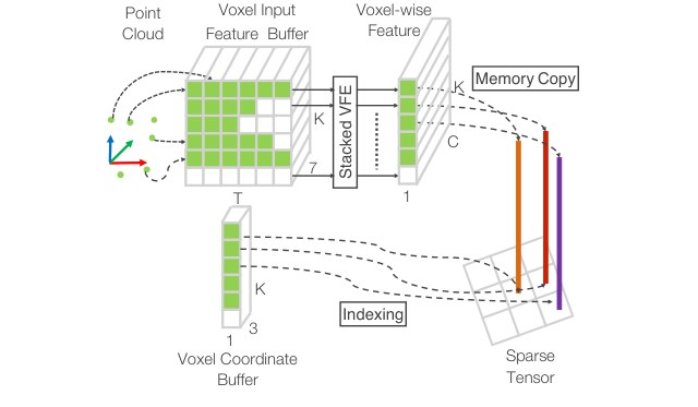
Figure 5: Illustration of efficient implementation.

图 5：高效实现示意。

2.3 Efficient Implementation

2.3 高效实现

GPUs are optimized for processing dense tensor structures. The problem with working directly with the point cloud is that the points are sparsely distributed across space and each voxel has a variable number of points. We devised a method that converts the point cloud into a dense tensor structure where stacked VFE operations can be processed in parallel across points and voxels.

GPU 适合处理密集张量结构。直接处理点云的困难在于：点在空间中稀疏分布，而且每个体素的点数不固定。我们设计了一种方法，把点云转换成密集张量，从而可以在点和体素两个维度上并行执行堆叠的 VFE 运算。

The method is summarized in Figure 5. We initialize a $K\times T\times 7$ dimensional tensor structure to store the voxel input feature buffer where $K$ is the maximum number of non-empty voxels, $T$ is the maximum number of points per voxel, and $7$ is the input encoding dimension for each point. The points are randomized before processing. For each point in the point cloud, we check if the corresponding voxel already exists. This lookup operation is done efficiently in $O(1)$ using a hash table where the voxel coordinate is used as the hash key. If the voxel is already initialized we insert the point to the voxel location if there are less than $T$ points, otherwise the point is ignored. If the voxel is not initialized, we initialize a new voxel, store its coordinate in the voxel coordinate buffer, and insert the point to this voxel location. The voxel input feature and coordinate buffers can be constructed via a single pass over the point list, therefore its complexity is $O(n)$. To further improve the memory/compute efficiency it is possible to only store a limited number of voxels ($K$) and ignore points coming from voxels with few points.

方法概要见图 5。我们初始化一个 $K\times T\times 7$ 维的张量作为体素输入特征缓冲区，其中 $K$ 是非空体素的最大数量，$T$ 是每个体素的最大点数，7 是每个点的输入编码维度。处理前先把点随机打乱。对点云中的每个点，检查它所对应的体素是否已经存在。这一查找用哈希表在 $O(1)$ 时间内完成，哈希键就是体素坐标。若体素已初始化，则在点数仍少于 $T$ 时把该点插入该体素，否则忽略该点。若体素尚未初始化，就新建一个体素，把它的坐标写入体素坐标缓冲区，再把该点插入。体素输入特征和坐标缓冲区可以在一遍扫描点列表后构建完成，复杂度为 $O(n)$。若要进一步节省显存和计算，也可以只保存有限个（$K$ 个）体素，并忽略来自点数很少的体素的点。

After the voxel input buffer is constructed, the stacked VFE only involves point level and voxel level dense operations which can be computed on a GPU in parallel. Note that, after concatenation operations in VFE, we reset the features corresponding to empty points to zero such that they do not affect the computed voxel features. Finally, using the stored coordinate buffer we reorganize the computed sparse voxel-wise structures to the dense voxel grid. The following convolutional middle layers and RPN operations work on a dense voxel grid which can be efficiently implemented on a GPU.

体素输入缓冲区构建完成后，堆叠 VFE 只涉及点和体素两个层级上的密集运算，可以在 GPU 上并行计算。需要注意的是，在 VFE 的拼接操作之后，我们把空位对应的特征重置为零，以免它们影响算得的体素特征。最后，借助保存的坐标缓冲区，把算得的稀疏体素结构重新组织到密集体素网格上。后续的卷积中间层和 RPN 都在密集体素网格上运算，可以在 GPU 上高效实现。

3 Training Details

3 训练细节

In this section, we explain the implementation details of the VoxelNet and the training procedure.

本节说明 VoxelNet 的实现细节和训练流程。

3.1 Network Details

3.1 网络细节

Our experimental setup is based on the LiDAR specifications of the KITTI dataset [11].

实验设置依据 KITTI 数据集[11]的激光雷达规格。

Car Detection For this task, we consider point clouds within the range of $[-3,1]\times[-40,40]\times[0,70.4]$ meters along Z, Y, X axis respectively. Points that are projected outside of image boundaries are removed [5]. We choose a voxel size of $v_{D}=0.4,v_{H}=0.2,v_{W}=0.2$ meters, which leads to $D^{\prime}=10$, $H^{\prime}=400$, $W^{\prime}=352$. We set $T=35$ as the maximum number of randomly sampled points in each non-empty voxel. We use two VFE layers $\textrm{VFE-1}(7,32)$ and $\textrm{VFE-2}(32,128)$. The final FCN maps VFE-2 output to $\mathbb{R}^{128}$. Thus our feature learning net generates a sparse tensor of shape $128\times 10\times 400\times 352$. To aggregate voxel-wise features, we employ three convolution middle layers sequentially as Conv3D(128, 64, 3, (2,1,1), (1,1,1)), Conv3D(64, 64, 3, (1,1,1), (0,1,1)), and Conv3D(64, 64, 3, (2,1,1), (1,1,1)), which yields a 4D tensor of size $64\times 2\times 400\times 352$. After reshaping, the input to RPN is a feature map of size $128\times 400\times 352$, where the dimensions correspond to channel, height, and width of the 3D tensor. Figure 4 illustrates the detailed network architecture for this task. Unlike [5], we use only one anchor size, $l^{a}=3.9,w^{a}=1.6,h^{a}=1.56$ meters, centered at $z_{c}^{a}=-1.0$ meters with two rotations, 0 and 90 degrees. Our anchor matching criteria is as follows: An anchor is considered as positive if it has the highest Intersection over Union (IoU) with a ground truth or its IoU with ground truth is above 0.6 (in bird’s eye view). An anchor is considered as negative if the IoU between it and all ground truth boxes is less than 0.45. We treat anchors as don’t care if they have $0.45\leq\textrm{IoU}\leq 0.6$ with any ground truth. We set $\alpha=1.5$ and $\beta=1$ in Eqn. 2.

车辆检测 该任务中，我们考虑沿 Z、Y、X 轴范围分别为 $[-3,1]\times[-40,40]\times[0,70.4]$ 米的点云。投影到图像边界之外的点会被去掉[5]。体素大小取 $v_{D}=0.4,v_{H}=0.2,v_{W}=0.2$ 米，于是 $D^{\prime}=10$，$H^{\prime}=400$，$W^{\prime}=352$。每个非空体素最多随机采样 $T=35$ 个点。我们使用两层 VFE：$\textrm{VFE-1}(7,32)$ 和 $\textrm{VFE-2}(32,128)$。最后的 FCN 把 VFE-2 的输出映射到 $\mathbb{R}^{128}$。因此特征学习网络产生形状为 $128\times 10\times 400\times 352$ 的稀疏张量。为汇聚体素级特征，我们依次使用三个卷积中间层：Conv3D(128, 64, 3, (2,1,1), (1,1,1))、Conv3D(64, 64, 3, (1,1,1), (0,1,1)) 和 Conv3D(64, 64, 3, (2,1,1), (1,1,1))，得到大小为 $64\times 2\times 400\times 352$ 的四维张量。变形之后，RPN 的输入是大小为 $128\times 400\times 352$ 的特征图，三个维度分别对应三维张量的通道、高和宽。图 4 给出了该任务的详细网络结构。与[5]不同，我们只使用一种锚框尺寸 $l^{a}=3.9,w^{a}=1.6,h^{a}=1.56$ 米，中心在 $z_{c}^{a}=-1.0$ 米，并取 0 度和 90 度两种旋转。锚框匹配规则如下：若某个锚框与某个真值框的交并比（IoU）最高，或其与真值框的 IoU（在鸟瞰视图中）高于 0.6，则视为正样本；若它与所有真值框的 IoU 都小于 0.45，则视为负样本；若它与任一真值框满足 $0.45\leq\textrm{IoU}\leq 0.6$，则视为 don't care。式 2 中取 $\alpha=1.5$、$\beta=1$。

Pedestrian and Cyclist Detection The input range[^1] is $[-3,1]\times[-20,20]\times[0,48]$ meters along Z, Y, X axis respectively. We use the same voxel size as for car detection, which yields $D=10$, $H=200$, $W=240$. We set $T=45$ in order to obtain more LiDAR points for better capturing shape information. The feature learning network and convolutional middle layers are identical to the networks used in the car detection task. For the RPN, we make one modification to block 1 in Figure 4 by changing the stride size in the first 2D convolution from 2 to 1. This allows finer resolution in anchor matching, which is necessary for detecting pedestrians and cyclists. We use anchor size $l^{a}=0.8,w^{a}=0.6,h^{a}=1.73$ meters centered at $z_{c}^{a}=-0.6$ meters with 0 and 90 degrees rotation for pedestrian detection and use anchor size $l^{a}=1.76,w^{a}=0.6,h^{a}=1.73$ meters centered at $z_{c}^{a}=-0.6$ with 0 and 90 degrees rotation for cyclist detection. The specific anchor matching criteria is as follows: We assign an anchor as postive if it has the highest IoU with a ground truth, or its IoU with ground truth is above 0.5. An anchor is considered as negative if its IoU with every ground truth is less than 0.35. For anchors having $0.35\leq\textrm{IoU}\leq 0.5$ with any ground truth, we treat them as don’t care.

行人和骑行者检测 输入范围是沿 Z、Y、X 轴的 $[-3,1]\times[-20,20]\times[0,48]$ 米。体素大小与车辆检测相同，于是 $D=10$，$H=200$，$W=240$。为了拿到更多激光雷达点以更好捕捉形状，我们取 $T=45$。特征学习网络和卷积中间层与车辆检测任务相同。对 RPN，我们只改动图 4 中的第 1 块：把第一个二维卷积的步长从 2 改成 1。这样锚框匹配的分辨率更细，对检测行人和骑行者是必要的。行人检测使用锚框尺寸 $l^{a}=0.8,w^{a}=0.6,h^{a}=1.73$ 米，中心在 $z_{c}^{a}=-0.6$ 米，旋转取 0 度和 90 度；骑行者检测使用 $l^{a}=1.76,w^{a}=0.6,h^{a}=1.73$ 米，中心同样在 $z_{c}^{a}=-0.6$，旋转同样取 0 度和 90 度。匹配规则如下：若某个锚框与某个真值框的 IoU 最高，或其与真值框的 IoU 高于 0.5，则标为正样本；若它与每个真值框的 IoU 都小于 0.35，则视为负样本；若它与任一真值框满足 $0.35\leq\textrm{IoU}\leq 0.5$，则视为 don't care。

During training, we use stochastic gradient descent (SGD) with learning rate 0.01 for the first 150 epochs and decrease the learning rate to 0.001 for the last 10 epochs. We use a batchsize of 16 point clouds.

训练时使用随机梯度下降（SGD），前 150 个 epoch 学习率为 0.01，最后 10 个 epoch 降到 0.001。批量大小为 16 帧点云。

3.2 Data Augmentation

3.2 数据增强

With less than 4000 training point clouds, training our network from scratch will inevitably suffer from overfitting. To reduce this issue, we introduce three different forms of data augmentation. The augmented training data are generated on-the-fly without the need to be stored on disk [20].

训练点云不足 4000 帧，若从头训练，网络难免过拟合。为缓解这一问题，我们引入三种数据增强。增强后的训练数据在线生成，不必存到磁盘上[20]。

Define set $\mathbf{M}=\{\mathbf{p}_{i}=[x_{i},y_{i},z_{i},r_{i}]^{T}\in\mathbb{R}^{4}\}_{i=1,\ldots,N}$ as the whole point cloud, consisting of $N$ points. We parameterize a 3D bouding box $\mathbf{b}_{i}$ as $(x_{c},y_{c},z_{c},l,w,h,\theta)$, where $x_{c},y_{c},z_{c}$ are center locations, $l,w,h$ are length, width, height, and $\theta$ is the yaw rotation around Z-axis. We define $\Omega_{i}=\{\mathbf{p}|x\in[x_{c}-l/2,x_{c}+l/2],y\in[y_{c}-w/2,y_{c}+w/2],z\in[z_{c}-h/2,z_{c}+h/2],\mathbf{p}\in\mathbf{M}\}$ as the set containing all LiDAR points within $\mathbf{b}_{i}$, where $\mathbf{p}=[x,y,z,r]$ denotes a particular LiDAR point in the whole set $\mathbf{M}$.

把整帧点云记为 $\mathbf{M}=\{\mathbf{p}_{i}=[x_{i},y_{i},z_{i},r_{i}]^{T}\in\mathbb{R}^{4}\}_{i=1,\ldots,N}$，共 $N$ 个点。三维边界框 $\mathbf{b}_{i}$ 参数化为 $(x_{c},y_{c},z_{c},l,w,h,\theta)$，其中 $x_{c},y_{c},z_{c}$ 是中心位置，$l,w,h$ 是长、宽、高，$\theta$ 是绕 Z 轴的偏航角。我们定义 $\Omega_{i}=\{\mathbf{p}|x\in[x_{c}-l/2,x_{c}+l/2],y\in[y_{c}-w/2,y_{c}+w/2],z\in[z_{c}-h/2,z_{c}+h/2],\mathbf{p}\in\mathbf{M}\}$ 为落在 $\mathbf{b}_{i}$ 内的全部激光雷达点，其中 $\mathbf{p}=[x,y,z,r]$ 表示全集 $\mathbf{M}$ 中的某个点。

The first form of data augmentation applies perturbation independently to each ground truth 3D bounding box together with those LiDAR points within the box. Specifically, around Z-axis we rotate $\mathbf{b}_{i}$ and the associated $\Omega_{i}$ with respect to $(x_{c},y_{c},z_{c})$ by a uniformally distributed random variable $\Delta\theta\in[-\pi/10,+\pi/10]$. Then we add a translation $(\Delta x,\Delta y,\Delta z)$ to the XYZ components of $\mathbf{b}_{i}$ and to each point in $\Omega_{i}$, where $\Delta x$, $\Delta y$, $\Delta z$ are drawn independently from a Gaussian distribution with mean zero and standard deviation 1.0. To avoid physically impossible outcomes, we perform a collision test between any two boxes after the perturbation and revert to the original if a collision is detected. Since the perturbation is applied to each ground truth box and the associated LiDAR points independently, the network is able to learn from substantially more variations than from the original training data.

第一种增强是对每个真值三维框及其内部的激光雷达点独立做扰动。具体来说，绕 Z 轴、相对于 $(x_{c},y_{c},z_{c})$，用均匀分布随机变量 $\Delta\theta\in[-\pi/10,+\pi/10]$ 旋转 $\mathbf{b}_{i}$ 及其对应的 $\Omega_{i}$。再给 $\mathbf{b}_{i}$ 的 XYZ 分量和 $\Omega_{i}$ 中每个点加上平移 $(\Delta x,\Delta y,\Delta z)$，其中 $\Delta x$、$\Delta y$、$\Delta z$ 独立取样自均值为 0、标准差为 1.0 的高斯分布。为避免出现物理上不可能的结果，扰动后对任意两个框做碰撞检测，一旦发生碰撞就恢复原状。由于扰动是对每个真值框及对应激光雷达点独立施加的，网络能学到比原始训练数据丰富得多的变化。

Secondly, we apply global scaling to all ground truth boxes $\mathbf{b}_{i}$ and to the whole point cloud $\mathbf{M}$. Specifically, we multiply the XYZ coordinates and the three dimensions of each $\mathbf{b}_{i}$, and the XYZ coordinates of all points in $\mathbf{M}$ with a random variable drawn from uniform distribution $[0.95,1.05]$. Introducing global scale augmentation improves robustness of the network for detecting objects with various sizes and distances as shown in image-based classification [35, 18] and detection tasks [12, 17].

第二种是对所有真值框 $\mathbf{b}_{i}$ 和整帧点云 $\mathbf{M}$ 做全局缩放。具体做法是：用从均匀分布 $[0.95,1.05]$ 中抽取的随机变量，去乘每个 $\mathbf{b}_{i}$ 的 XYZ 坐标和三个尺寸，以及 $\mathbf{M}$ 中所有点的 XYZ 坐标。引入全局尺度增强，能提高网络检测不同大小、不同距离物体时的稳健性，这在基于图像的分类[35, 18]和检测[12, 17]中已有体现。

Finally, we apply global rotation to all ground truth boxes $\mathbf{b}_{i}$ and to the whole point cloud $\mathbf{M}$. The rotation is applied along Z-axis and around $(0,0,0)$. The global rotation offset is determined by sampling from uniform distribution $[-\pi/4,+\pi/4]$. By rotating the entire point cloud, we simulate the vehicle making a turn.

最后，我们对所有真值框 $\mathbf{b}_{i}$ 和整帧点云 $\mathbf{M}$ 做全局旋转。旋转绕 Z 轴、以 $(0,0,0)$ 为中心，全局旋转偏移取样自均匀分布 $[-\pi/4,+\pi/4]$。旋转整帧点云，相当于模拟车辆转弯。

Method	Modality	Car	Pedestrian	Cyclist
Easy	Moderate	Hard	Easy	Moderate	Hard	Easy	Moderate	Hard
Mono3D [3]	Mono	5.22	5.19	4.13	N/A	N/A	N/A	N/A	N/A	N/A
3DOP [4]	Stereo	12.63	9.49	7.59	N/A	N/A	N/A	N/A	N/A	N/A
VeloFCN [22]	LiDAR	40.14	32.08	30.47	N/A	N/A	N/A	N/A	N/A	N/A
MV (BV+FV) [5]	LiDAR	86.18	77.32	76.33	N/A	N/A	N/A	N/A	N/A	N/A
MV (BV+FV+RGB) [5]	LiDAR+Mono	86.55	78.10	76.67	N/A	N/A	N/A	N/A	N/A	N/A
HC-baseline	LiDAR	88.26	78.42	77.66	58.96	53.79	51.47	63.63	42.75	41.06
VoxelNet	LiDAR	89.60	84.81	78.57	65.95	61.05	56.98	74.41	52.18	50.49

Table 1: Performance comparison in bird’s eye view detection: average precision (in %) on KITTI validation set.

方法	模态	汽车			行人			骑行者
		简单	中等	困难	简单	中等	困难	简单	中等	困难
Mono3D [3]	单目	5.22	5.19	4.13	N/A	N/A	N/A	N/A	N/A	N/A
3DOP [4]	双目	12.63	9.49	7.59	N/A	N/A	N/A	N/A	N/A	N/A
VeloFCN [22]	激光雷达	40.14	32.08	30.47	N/A	N/A	N/A	N/A	N/A	N/A
MV (BV+FV) [5]	激光雷达	86.18	77.32	76.33	N/A	N/A	N/A	N/A	N/A	N/A
MV (BV+FV+RGB) [5]	激光雷达+单目	86.55	78.10	76.67	N/A	N/A	N/A	N/A	N/A	N/A
HC-baseline	激光雷达	88.26	78.42	77.66	58.96	53.79	51.47	63.63	42.75	41.06
VoxelNet	激光雷达	89.60	84.81	78.57	65.95	61.05	56.98	74.41	52.18	50.49

表 1：鸟瞰检测性能对比：KITTI 验证集上的平均精度（%）。

Method	Modality	Car	Pedestrian	Cyclist
Easy	Moderate	Hard	Easy	Moderate	Hard	Easy	Moderate	Hard
Mono3D [3]	Mono	2.53	2.31	2.31	N/A	N/A	N/A	N/A	N/A	N/A
3DOP [4]	Stereo	6.55	5.07	4.10	N/A	N/A	N/A	N/A	N/A	N/A
VeloFCN [22]	LiDAR	15.20	13.66	15.98	N/A	N/A	N/A	N/A	N/A	N/A
MV (BV+FV) [5]	LiDAR	71.19	56.60	55.30	N/A	N/A	N/A	N/A	N/A	N/A
MV (BV+FV+RGB) [5]	LiDAR+Mono	71.29	62.68	56.56	N/A	N/A	N/A	N/A	N/A	N/A
HC-baseline	LiDAR	71.73	59.75	55.69	43.95	40.18	37.48	55.35	36.07	34.15
VoxelNet	LiDAR	81.97	65.46	62.85	57.86	53.42	48.87	67.17	47.65	45.11

Table 2: Performance comparison in 3D detection: average precision (in %) on KITTI validation set.

方法	模态	汽车			行人			骑行者
		简单	中等	困难	简单	中等	困难	简单	中等	困难
Mono3D [3]	单目	2.53	2.31	2.31	N/A	N/A	N/A	N/A	N/A	N/A
3DOP [4]	双目	6.55	5.07	4.10	N/A	N/A	N/A	N/A	N/A	N/A
VeloFCN [22]	激光雷达	15.20	13.66	15.98	N/A	N/A	N/A	N/A	N/A	N/A
MV (BV+FV) [5]	激光雷达	71.19	56.60	55.30	N/A	N/A	N/A	N/A	N/A	N/A
MV (BV+FV+RGB) [5]	激光雷达+单目	71.29	62.68	56.56	N/A	N/A	N/A	N/A	N/A	N/A
HC-baseline	激光雷达	71.73	59.75	55.69	43.95	40.18	37.48	55.35	36.07	34.15
VoxelNet	激光雷达	81.97	65.46	62.85	57.86	53.42	48.87	67.17	47.65	45.11

表 2：三维检测性能对比：KITTI 验证集上的平均精度（%）。

4 Experiments

4 实验

We evaluate VoxelNet on the KITTI 3D object detection benchmark [11] which contains 7,481 training images/point clouds and 7,518 test images/point clouds, covering three categories: Car, Pedestrian, and Cyclist. For each class, detection outcomes are evaluated based on three difficulty levels: easy, moderate, and hard, which are determined according to the object size, occlusion state, and truncation level. Since the ground truth for the test set is not available and the access to the test server is limited, we conduct comprehensive evaluation using the protocol described in [4, 3, 5] and subdivide the training data into a training set and a validation set, which results in 3,712 data samples for training and 3,769 data samples for validation. The split avoids samples from the same sequence being included in both the training and the validation set [3]. Finally we also present the test results using the KITTI server.

我们在 KITTI 三维目标检测基准[11]上评估 VoxelNet。该基准包含 7,481 组训练图像／点云和 7,518 组测试图像／点云，覆盖三类：汽车、行人和骑行者。每一类的检测结果按三种难度评估：简单、中等和困难，划分依据是物体尺寸、遮挡状态和截断程度。由于测试集没有公开真值，且测试服务器访问受限，我们按照[4, 3, 5]的协议做全面评估，把训练数据再分成训练集和验证集，分别有 3,712 和 3,769 个样本。这一划分避免同一序列的样本同时出现在训练集和验证集中[3]。最后我们也给出通过 KITTI 服务器得到的测试结果。

For the Car category, we compare the proposed method with several top-performing algorithms, including image based approaches: Mono3D [3] and 3DOP [4]; LiDAR based approaches: VeloFCN [22] and 3D-FCN [21]; and a multi-modal approach MV [5]. Mono3D [3], 3DOP [4] and MV [5] use a pre-trained model for initialization whereas we train VoxelNet from scratch using only the LiDAR data provided in KITTI.

对汽车这一类，我们把所提方法与若干表现最好的算法比较，包括基于图像的 Mono3D[3] 和 3DOP[4]，基于激光雷达的 VeloFCN[22] 和 3D-FCN[21]，以及多模态方法 MV[5]。Mono3D[3]、3DOP[4] 和 MV[5] 用预训练模型做初始化，而我们只用 KITTI 提供的激光雷达数据从头训练 VoxelNet。

To analyze the importance of end-to-end learning, we implement a strong baseline that is derived from the VoxelNet architecture but uses hand-crafted features instead of the proposed feature learning network. We call this model the hand-crafted baseline (HC-baseline). HC-baseline uses the bird’s eye view features described in [5] which are computed at $0.1$m resolution. Different from [5], we increase the number of height channels from 4 to 16 to capture more detailed shape information– further increasing the number of height channels did not lead to performance improvement. We replace the convolutional middle layers of VoxelNet with similar size 2D convolutional layers, which are Conv2D(16, 32, 3, 1, 1), Conv2D(32, 64, 3, 2, 1), Conv2D(64, 128, 3, 1, 1). Finally RPN is identical in VoxelNet and HC-baseline. The total number of parameters in HC-baseline and VoxelNet are very similar. We train the HC-baseline using the same training procedure and data augmentation described in Section 3.

为分析端到端学习的重要性，我们实现了一个强基线：整体仍来自 VoxelNet 架构，但用手工特征替换所提出的特征学习网络，称为手工特征基线（HC-baseline）。HC-baseline 使用[5]中描述的鸟瞰特征，分辨率为 0.1 米。与[5]不同的是，我们把高度通道数从 4 增加到 16，以捕捉更细致的形状信息——再继续增加高度通道并未带来性能提升。我们用相近规模的二维卷积层替换 VoxelNet 的卷积中间层，分别为 Conv2D(16, 32, 3, 1, 1)、Conv2D(32, 64, 3, 2, 1)、Conv2D(64, 128, 3, 1, 1)。RPN 则与 VoxelNet 完全相同。HC-baseline 和 VoxelNet 的参数总量非常接近。我们用第 3 节描述的同一套训练流程和数据增强来训练 HC-baseline。

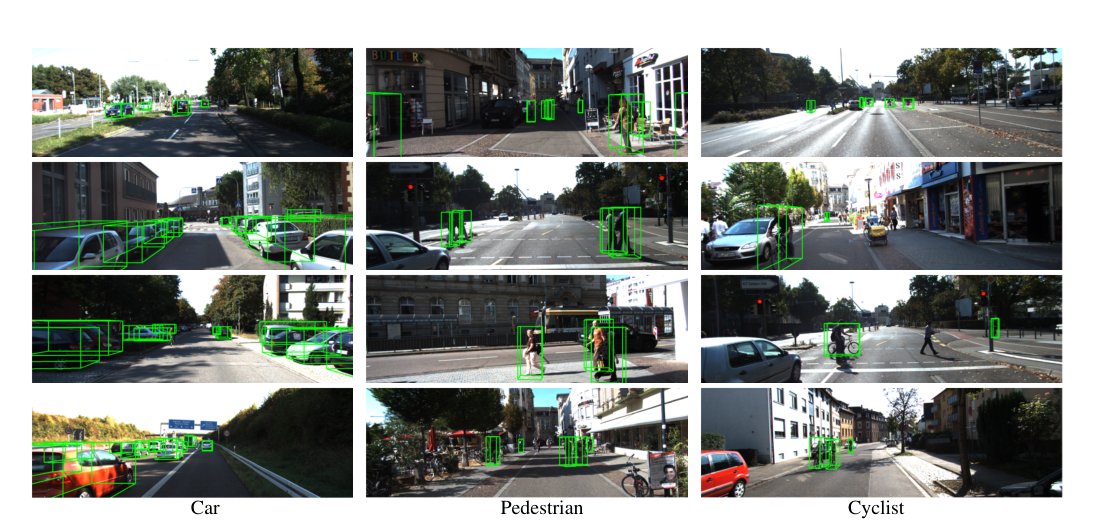
Figure 6: Qualitative results. For better visualization 3D boxes detected using LiDAR are projected on to the RGB images.

图 6：定性结果。为便于观察，用激光雷达检出的三维框被投影到 RGB 图像上。

4.1 Evaluation on KITTI Validation Set

4.1 在 KITTI 验证集上的评估

Metrics

We follow the official KITTI evaluation protocol, where the IoU threshold is 0.7 for class Car and is 0.5 for class Pedestrian and Cyclist. The IoU threshold is the same for both bird’s eye view and full 3D evaluation. We compare the methods using the average precision (AP) metric.

指标

我们遵循官方 KITTI 评估协议：汽车类的 IoU 阈值为 0.7，行人与骑行者类为 0.5。鸟瞰评估和完整三维评估使用相同的 IoU 阈值。比较时采用平均精度（AP）指标。

Evaluation in Bird’s Eye View

The evaluation result is presented in Table 1. VoxelNet consistently outperforms all the competing approaches across all three difficulty levels. HC-baseline also achieves satisfactory performance compared to the state-of-the-art [5], which shows that our base region proposal network (RPN) is effective. For Pedestrian and Cyclist detection tasks in bird’s eye view, we compare the proposed VoxelNet with HC-baseline. VoxelNet yields substantially higher AP than the HC-baseline for these more challenging categories, which shows that end-to-end learning is essential for point-cloud based detection.

鸟瞰评估

评估结果见表 1。VoxelNet 在全部三个难度上都持续超过所有对照方法。HC-baseline 相对当时的领先方法[5]也有不错表现，说明我们的基础区域提议网络（RPN）是有效的。在鸟瞰视图的行人和骑行者检测上，我们把 VoxelNet 与 HC-baseline 比较。在这两类更具挑战的类别上，VoxelNet 的 AP 明显高于 HC-baseline，说明端到端学习对基于点云的检测至关重要。

We would like to note that [21] reported 88.9%, 77.3%, and 72.7% for easy, moderate, and hard levels respectively, but these results are obtained based on a different split of 6,000 training frames and $\sim$1,500 validation frames, and they are not directly comparable with algorithms in Table 1. Therefore, we do not include these results in the table.

需要说明的是，[21]报告的简单、中等、困难档结果分别为 88.9%、77.3% 和 72.7%，但这些数字来自分成 6,000 帧训练和约 1,500 帧验证的另一种划分，不能与表 1 中的算法直接比较。因此我们没有把这些结果列入表中。

Evaluation in 3D

Compared to the bird’s eye view detection, which requires only accurate localization of objects in the 2D plane, 3D detection is a more challenging task as it requires finer localization of shapes in 3D space. Table 2 summarizes the comparison. For the class Car, VoxelNet significantly outperforms all other approaches in AP across all difficulty levels. Specifically, using only LiDAR, VoxelNet significantly outperforms the state-of-the-art method MV (BV+FV+RGB) [5] based on LiDAR+RGB, by 10.68%, 2.78% and 6.29% in easy, moderate, and hard levels respectively. HC-baseline achieves similar accuracy to the MV [5] method.

三维评估

鸟瞰检测只要求在二维平面上准确定位物体，三维检测则更难，因为它要求在三维空间中更精细地定位形状。表 2 汇总了对比结果。对汽车类，VoxelNet 在全部难度上的 AP 都明显超过其他方法。具体而言，仅用激光雷达，VoxelNet 就比基于激光雷达加 RGB 的当时领先方法 MV（BV+FV+RGB）[5]在简单、中等、困难档上分别高出 10.68%、2.78% 和 6.29%。HC-baseline 的精度与 MV[5]相近。

As in the bird’s eye view evaluation, we also compare VoxelNet with HC-baseline on 3D Pedestrian and Cyclist detection. Due to the high variation in 3D poses and shapes, successful detection of these two categories requires better 3D shape representation. As shown in Table 2 the improved performance of VoxelNet is emphasized for more challenging 3D detection tasks (from $\sim$8% improvement in bird’s eye view to $\sim$12% improvement on 3D detection) which suggests that VoxelNet is more effective in capturing 3D shape information than hand-crafted features.

与鸟瞰评估一样，我们也在三维行人和骑行者检测上把 VoxelNet 与 HC-baseline 比较。这两类的三维姿态和形状变化很大，要成功检测就需要更好的三维形状表示。如表 2 所示，VoxelNet 的提升在更具挑战的三维检测任务上更加明显（从鸟瞰上约 8 个百分点的提升，扩大到三维检测上约 12 个百分点），说明 VoxelNet 比手工特征更能捕捉三维形状信息。

4.2 Evaluation on KITTI Test Set

4.2 在 KITTI 测试集上的评估

We evaluated VoxelNet on the KITTI test set by submitting detection results to the official server. The results are summarized in Table 3. VoxelNet, significantly outperforms the previously published state-of-the-art [5] in all the tasks (bird’s eye view and 3D detection) and all difficulties. We would like to note that many of the other leading methods listed in KITTI benchmark use both RGB images and LiDAR point clouds whereas VoxelNet uses only LiDAR.

我们把检测结果提交到官方服务器，在 KITTI 测试集上评估 VoxelNet。结果汇总于表 3。在全部任务（鸟瞰和三维检测）和全部难度上，VoxelNet 都明显超过此前已发表的领先方法[5]。需要指出的是，KITTI 基准上许多其他靠前的方法同时使用 RGB 图像和激光雷达点云，而 VoxelNet 只用激光雷达。

We present several 3D detection examples in Figure 6. For better visualization 3D boxes detected using LiDAR are projected on to the RGB images. As shown, VoxelNet provides highly accurate 3D bounding boxes in all categories.

图 6 给出若干三维检测示例。为便于观察，用激光雷达检出的三维框被投影到 RGB 图像上。可以看到，VoxelNet 在所有类别上都给出了相当准确的三维边界框。

The inference time for the VoxelNet is 225ms where the voxel input feature computation takes 5ms, feature learning net takes 20ms, convolutional middle layers take 170ms, and region proposal net takes 30ms on a TitanX GPU and 1.7Ghz CPU.

VoxelNet 的推理时间为 225 毫秒，其中体素输入特征计算占 5 毫秒，特征学习网络占 20 毫秒，卷积中间层占 170 毫秒，区域提议网络占 30 毫秒，测试平台为 TitanX GPU 和 1.7GHz CPU。

Benchmark	Easy	Moderate	Hard
Car (3D Detection)	77.47	65.11	57.73
Car (Bird’s Eye View)	89.35	79.26	77.39
Pedestrian (3D Detection)	39.48	33.69	31.51
Pedestrian (Bird’s Eye View)	46.13	40.74	38.11
Cyclist (3D Detection)	61.22	48.36	44.37
Cyclist (Bird’s Eye View)	66.70	54.76	50.55

Table 3: Performance evaluation on KITTI test set.

基准	简单	中等	困难
汽车（三维检测）	77.47	65.11	57.73
汽车（鸟瞰）	89.35	79.26	77.39
行人（三维检测）	39.48	33.69	31.51
行人（鸟瞰）	46.13	40.74	38.11
骑行者（三维检测）	61.22	48.36	44.37
骑行者（鸟瞰）	66.70	54.76	50.55

表 3：KITTI 测试集上的性能评估。

5 Conclusion

5 结论

Most existing methods in LiDAR-based 3D detection rely on hand-crafted feature representations, for example, a bird’s eye view projection. In this paper, we remove the bottleneck of manual feature engineering and propose VoxelNet, a novel end-to-end trainable deep architecture for point cloud based 3D detection. Our approach can operate directly on sparse 3D points and capture 3D shape information effectively. We also present an efficient implementation of VoxelNet that benefits from point cloud sparsity and parallel processing on a voxel grid. Our experiments on the KITTI car detection task show that VoxelNet outperforms state-of-the-art LiDAR based 3D detection methods by a large margin. On more challenging tasks, such as 3D detection of pedestrians and cyclists, VoxelNet also demonstrates encouraging results showing that it provides a better 3D representation. Future work includes extending VoxelNet for joint LiDAR and image based end-to-end 3D detection to further improve detection and localization accuracy.

现有的大多数基于激光雷达的三维检测方法依赖手工特征表示，例如鸟瞰投影。本文去掉人工特征工程这一瓶颈，提出 VoxelNet：一种面向点云三维检测的新型可端到端训练深度架构。该方法可以直接处理稀疏三维点，并有效捕捉三维形状信息。我们也给出了 VoxelNet 的一种高效实现，既利用点云稀疏性，又能在体素网格上并行计算。在 KITTI 车辆检测任务上的实验表明，VoxelNet 大幅超过当时最强的纯激光雷达三维检测方法。在行人和骑行者三维检测这类更难的任务上，VoxelNet 同样给出了积极结果，说明它能提供更好的三维表示。后续工作包括把 VoxelNet 扩展到激光雷达与图像联合的端到端三维检测，以进一步提高检测和定位精度。

Acknowledgement:

We are grateful to our colleagues Russ Webb, Barry Theobald, and Jerremy Holland for their valuable input.

致谢

感谢同事 Russ Webb、Barry Theobald 和 Jerremy Holland 提出的宝贵意见。

References

参考文献

[1] P. Bariya and K. Nishino. Scale-hierarchical 3d object recognition in cluttered scenes. In 2010 IEEE Computer Society Conference on Computer Vision and Pattern Recognition , pages 1657–1664, 2010.

[2] L. Bo, X. Ren, and D. Fox. Depth Kernel Descriptors for Object Recognition. In IROS , September 2011.

[3] X. Chen, K. Kundu, Z. Zhang, H. Ma, S. Fidler, and R. Urtasun. Monocular 3d object detection for autonomous driving. In IEEE CVPR , 2016.

[4] X. Chen, K. Kundu, Y. Zhu, A. Berneshawi, H. Ma, S. Fidler, and R. Urtasun. 3d object proposals for accurate object class detection. In NIPS , 2015.

[5] X. Chen, H. Ma, J. Wan, B. Li, and T. Xia. Multi-view 3d object detection network for autonomous driving. In IEEE CVPR , 2017.

[6] C. Choi, Y. Taguchi, O. Tuzel, M. Y. Liu, and S. Ramalingam. Voting-based pose estimation for robotic assembly using a 3d sensor. In 2012 IEEE International Conference on Robotics and Automation , pages 1724–1731, 2012.

[7] C. S. Chua and R. Jarvis. Point signatures: A new representation for 3d object recognition. International Journal of Computer Vision , 25(1):63–85, Oct 1997.

[8] C. Dorai and A. K. Jain. Cosmos-a representation scheme for 3d free-form objects. IEEE Transactions on Pattern Analysis and Machine Intelligence , 19(10):1115–1130, 1997.

[9] M. Engelcke, D. Rao, D. Z. Wang, C. H. Tong, and I. Posner. Vote3deep: Fast object detection in 3d point clouds using efficient convolutional neural networks. In 2017 IEEE International Conference on Robotics and Automation (ICRA) , pages 1355–1361, May 2017.

[10] M. Enzweiler and D. M. Gavrila. A multilevel mixture-of-experts framework for pedestrian classification. IEEE Transactions on Image Processing , 20(10):2967–2979, Oct 2011.

[11] A. Geiger, P. Lenz, and R. Urtasun. Are we ready for autonomous driving? the kitti vision benchmark suite. In Conference on Computer Vision and Pattern Recognition (CVPR) , 2012.

[12] R. Girshick. Fast r-cnn. In Proceedings of the 2015 IEEE International Conference on Computer Vision (ICCV) , ICCV ’15, 2015.

[13] R. Girshick, J. Donahue, T. Darrell, and J. Malik. Rich feature hierarchies for accurate object detection and semantic segmentation. In Proceedings of the IEEE conference on computer vision and pattern recognition , pages 580–587, 2014.

[14] R. Gomez-Ojeda, J. Briales, and J. Gonzalez-Jimenez. Pl-svo: Semi-direct monocular visual odometry by combining points and line segments. In 2016 IEEE/RSJ International Conference on Intelligent Robots and Systems (IROS) , pages 4211–4216, Oct 2016.

[15] A. Gonzalez, G. Villalonga, J. Xu, D. Vazquez, J. Amores, and A. Lopez. Multiview random forest of local experts combining rgb and lidar data for pedestrian detection. In IEEE Intelligent Vehicles Symposium (IV) , 2015.

[16] A. González, D. Vázquez, A. M. López, and J. Amores. On-board object detection: Multicue, multimodal, and multiview random forest of local experts. IEEE Transactions on Cybernetics , 47(11):3980–3990, Nov 2017.

[17] K. He, X. Zhang, S. Ren, and J. Sun. Deep residual learning for image recognition. In 2016 IEEE Conference on Computer Vision and Pattern Recognition (CVPR) , pages 770–778, June 2016.

[18] A. G. Howard. Some improvements on deep convolutional neural network based image classification. CoRR , abs/1312.5402, 2013.

[19] A. E. Johnson and M. Hebert. Using spin images for efficient object recognition in cluttered 3d scenes. IEEE Transactions on Pattern Analysis and Machine Intelligence , 21(5):433–449, 1999.

[20] A. Krizhevsky, I. Sutskever, and G. E. Hinton. Imagenet classification with deep convolutional neural networks. In F. Pereira, C. J. C. Burges, L. Bottou, and K. Q. Weinberger, editors, Advances in Neural Information Processing Systems 25 , pages 1097–1105. Curran Associates, Inc., 2012.

[21] B. Li. 3d fully convolutional network for vehicle detection in point cloud. In IROS , 2017.

[22] B. Li, T. Zhang, and T. Xia. Vehicle detection from 3d lidar using fully convolutional network. In Robotics: Science and Systems , 2016.

[23] T. Lin, P. Goyal, R. B. Girshick, K. He, and P. Dollár. Focal loss for dense object detection. IEEE ICCV , 2017.

[24] W. Liu, D. Anguelov, D. Erhan, C. Szegedy, S. Reed, C.-Y. Fu, and A. C. Berg. Ssd: Single shot multibox detector. In ECCV , pages 21–37, 2016.

[25] A. Mian, M. Bennamoun, and R. Owens. On the repeatability and quality of keypoints for local feature-based 3d object retrieval from cluttered scenes. International Journal of Computer Vision , 89(2):348–361, Sep 2010.

[26] Y.-J. Oh and Y. Watanabe. Development of small robot for home floor cleaning. In Proceedings of the 41st SICE Annual Conference. SICE 2002. , volume 5, pages 3222–3223 vol.5, Aug 2002.

[27] Y. Park, V. Lepetit, and W. Woo. Multiple 3d object tracking for augmented reality. In 2008 7th IEEE/ACM International Symposium on Mixed and Augmented Reality , pages 117–120, Sept 2008.

[28] C. Premebida, J. Carreira, J. Batista, and U. Nunes. Pedestrian detection combining RGB and dense LIDAR data. In IROS , pages 0–1. IEEE, Sep 2014.

[29] C. R. Qi, H. Su, K. Mo, and L. J. Guibas. Pointnet: Deep learning on point sets for 3d classification and segmentation. Proc. Computer Vision and Pattern Recognition (CVPR), IEEE , 2017.

[30] C. R. Qi, L. Yi, H. Su, and L. J. Guibas. Pointnet++: Deep hierarchical feature learning on point sets in a metric space. arXiv preprint arXiv:1706.02413 , 2017.

[31] J. Redmon and A. Farhadi. YOLO9000: better, faster, stronger. In IEEE Conference on Computer Vision and Pattern Recognition (CVPR) , 2017.

[32] S. Ren, K. He, R. Girshick, and J. Sun. Faster r-cnn: Towards real-time object detection with region proposal networks. In Advances in Neural Information Processing Systems 28 , pages 91–99. 2015.

[33] R. B. Rusu, N. Blodow, and M. Beetz. Fast point feature histograms (fpfh) for 3d registration. In 2009 IEEE International Conference on Robotics and Automation , pages 3212–3217, 2009.

[34] J. Shotton, A. Fitzgibbon, M. Cook, T. Sharp, M. Finocchio, R. Moore, A. Kipman, and A. Blake. Real-time human pose recognition in parts from single depth images. In CVPR 2011 , pages 1297–1304, 2011.

[35] K. Simonyan and A. Zisserman. Very deep convolutional networks for large-scale image recognition. CoRR , abs/1409.1556, 2014.

[36] S. Song and M. Chandraker. Joint sfm and detection cues for monocular 3d localization in road scenes. In IEEE Conference on Computer Vision and Pattern Recognition (CVPR) , pages 3734–3742, June 2015.

[37] S. Song and J. Xiao. Sliding shapes for 3d object detection in depth images. In European Conference on Computer Vision, Proceedings , pages 634–651, Cham, 2014. Springer International Publishing.

[38] S. Song and J. Xiao. Deep Sliding Shapes for amodal 3D object detection in RGB-D images. In CVPR , 2016.

[39] F. Stein and G. Medioni. Structural indexing: efficient 3-d object recognition. IEEE Transactions on Pattern Analysis and Machine Intelligence , 14(2):125–145, 1992.

[40] O. Tuzel, M.-Y. Liu, Y. Taguchi, and A. Raghunathan. Learning to rank 3d features. In 13th European Conference on Computer Vision, Proceedings, Part I , pages 520–535, 2014.

[41] D. Z. Wang and I. Posner. Voting for voting in online point cloud object detection. In Proceedings of Robotics: Science and Systems , Rome, Italy, July 2015.

[42] Y. Xiang, W. Choi, Y. Lin, and S. Savarese. Data-driven 3d voxel patterns for object category recognition. In Proceedings of the IEEE International Conference on Computer Vision and Pattern Recognition , 2015.

[43] M. Z. Zia, M. Stark, B. Schiele, and K. Schindler. Detailed 3d representations for object recognition and modeling. IEEE Transactions on Pattern Analysis and Machine Intelligence , 35(11):2608–2623, 2013.

[44] M. Z. Zia, M. Stark, and K. Schindler. Are cars just 3d boxes? jointly estimating the 3d shape of multiple objects. In 2014 IEEE Conference on Computer Vision and Pattern Recognition , pages 3678–3685, June 2014.