VoxCeleb: A Large-Scale Speaker Identification Dataset
VoxCeleb: a large-scale speaker identification dataset
Abstract
摘要
Most existing datasets for speaker identification contain samples obtained under quite constrained conditions, and are usually hand-annotated, hence limited in size. The goal of this paper is to generate a large scale text-independent speaker identification dataset collected ‘in the wild’.
现有的说话人识别数据集,样本多半是在相当受控的条件下取得的,并且通常依赖人工标注,因此规模有限。本文的目标是构建一份在“野外”采集的大规模文本无关说话人识别数据集。
We make two contributions. First, we propose a fully automated pipeline based on computer vision techniques to create the dataset from open-source media. Our pipeline involves obtaining videos from YouTube; performing active speaker verification using a two-stream synchronization Convolutional Neural Network (CNN), and confirming the identity of the speaker using CNN based facial recognition. We use this pipeline to curate VoxCeleb which contains hundreds of thousands of ‘real world’ utterances for over 1,000 celebrities.
我们有两项贡献。第一,我们提出一条完全自动的流水线,借助计算机视觉技术从公开媒体中创建数据集。流水线包括从 YouTube 获取视频;用双流同步卷积神经网络(CNN)做主动说话人核验;再用基于 CNN 的人脸识别确认说话人身份。我们用这条流水线整理出 VoxCeleb,其中包含一千多位公众人物的数十万段“真实世界”话语。
Our second contribution is to apply and compare various state of the art speaker identification techniques on our dataset to establish baseline performance. We show that a CNN based architecture obtains the best performance for both identification and verification.
第二项贡献是在该数据集上应用并比较多种当时最先进的说话人识别方法,以建立基线表现。结果表明,基于 CNN 的架构在识别和验证两项任务上都取得了最好的成绩。
Index Terms: speaker identification, speaker verification, large-scale, dataset, convolutional neural network
关键词:说话人识别,说话人验证,大规模,数据集,卷积神经网络
- Introduction
- 引言
Speaker recognition under noisy and unconstrained conditions is an extremely challenging topic. Applications of speaker recognition are many and varied, ranging from authentication in high-security systems and forensic tests, to searching for persons in large corpora of speech data. All such tasks require high speaker recognition performance under ‘real world’ conditions. This is an extremely difficult task due to both extrinsic and intrinsic variations; extrinsic variations include background chatter and music, laughter, reverberation, channel and microphone effects; while intrinsic variations are factors inherent to the speaker themself such as age, accent, emotion, intonation and manner of speaking, amongst others [1].
在噪声和无约束条件下做说话人识别,是一项极具挑战的课题。说话人识别的应用又多又杂,从高安全系统中的认证、法庭取证,到在大规模语音语料中查找特定的人,都要求系统在“真实世界”条件下仍有很高的识别性能。这件事非常困难,因为同时存在外部和内部变化:外部变化包括背景聊天和音乐、笑声、混响、信道和麦克风效应;内部变化则是说话人自身的因素,例如年龄、口音、情绪、语调和说话方式等 [1]。
Deep Convolutional Neural Networks (CNNs) have given rise to substantial improvements in speech recognition, computer vision and related fields due to their ability to deal with real world, noisy datasets without the need for handcrafted features [2, 3, 4]. One of the most important ingredients for the success of such methods, however, is the availability of large training datasets.
深度卷积神经网络(CNN)已经在语音识别、计算机视觉及相关领域带来了显著进步,因为它们能够处理真实世界中的嘈杂数据,而不需要手工特征 [2, 3, 4]。不过,这类方法成功的一个最重要条件,仍是要有大规模训练数据。
Unfortunately, large-scale public datasets in the field of speaker identification with unconstrained speech samples are lacking. While large-scale evaluations are held regularly by the National Institute of Standards in Technology (NIST), these datasets are not freely available to the research community. The only freely available dataset curated from multimedia is the Speakers in the Wild (SITW) dataset [5], which contains speech samples of 299 speakers across unconstrained or ‘wild’ conditions. This is a valuable dataset, but to create it the speech samples have been hand-annotated. Scaling it further, for example to thousands of speakers across tens of thousands of utterances, would require the use of a service such as Amazon Mechanical Turk (AMT). In the computer vision community AMT like services have been used to produce very large-scale datasets, such as ImageNet [6].
遗憾的是,说话人识别领域仍缺少带无约束语音样本的大规模公开数据集。美国国家标准与技术研究院(NIST)虽然定期组织大规模评测,但这些数据并不能免费提供给研究社区。目前唯一从多媒体中整理、并可免费获取的,是 Speakers in the Wild(SITW)数据集 [5],它包含 299 位说话人在无约束或“野外”条件下的语音样本。这份数据很有价值,但其中的语音是人工标注的。若要继续扩大,例如到数千位说话人、数万段话语,就几乎需要借助 Amazon Mechanical Turk(AMT)一类服务。在计算机视觉社区,类似 AMT 的服务已被用来做出 ImageNet 这样的超大规模数据集 [6]。
This paper has two goals. The first is to propose a fully automated and scalable pipeline for creating a large-scale ‘real world’ speaker identification dataset. By using visual active speaker identification and face verification, our method circumvents the need for human annotation completely. We use this method to curate VoxCeleb, a large-scale dataset with hundreds of utterances for over a thousand speakers. The second goal is to investigate different architectures and techniques for training deep CNNs on spectrograms extracted directly from the raw audio files with very little pre-processing, and compare our results on this new dataset with more traditional state-of-the-art methods.
本文有两个目标。第一,提出一条完全自动、可扩展的流水线,用来创建大规模“真实世界”说话人识别数据集。通过视觉上的主动说话人识别和人脸验证,我们的方法完全绕开了人工标注。我们用该方法整理出 VoxCeleb,这是一份覆盖一千多位说话人、每人有数百段话语的大规模数据集。第二个目标是研究不同的架构和技术,以便在几乎不做预处理的情况下,直接从原始音频提取的语谱图上训练深度 CNN,并在这份新数据上把我们的结果与更传统的先进方法作比较。
VoxCeleb can be used for both speaker identification and verification. Speaker identification involves determining which speaker has produced a given utterance, if this is performed for a closed set of speakers then the task is similar to that of multi-class classification. Speaker verification on the other hand involves determining whether there is a match between a given utterance and a target model. We provide baselines for both tasks.
VoxCeleb 既可用于说话人识别,也可用于说话人验证。说话人识别要判断一段话语是由哪一位说话人发出的;若在封闭说话人集合上进行,任务便类似于多类分类。说话人验证则要判断一段给定话语与目标模型是否匹配。我们为这两项任务都提供了基线。
The dataset can be downloaded from http://www.robots.ox.ac.uk/~vgg/data/voxceleb.
- Related Works
- 相关工作
For a long time, speaker identification was the domain of Gaussian Mixture Models (GMMs) trained on low dimensional feature vectors [7, 8]. The state of the art in more recent times involves both the use of joint factor analysis (JFA) based methods which model speaker and channel subspaces separately [9], and i-vectors which attempt to model both subspaces into a single compact, low-dimensional space [10]. Although state of the art in speaker recognition tasks, these methods all have one thing in common – they rely on a low dimensional representation of the audio input, such as Mel Frequency Cepstrum Coefficients (MFCCs). However, not only does the performance of MFCCs degrade rapidly in real world noise [11, 12], but by focusing only on the overall spectral envelope of short frames, MFCCs may be lacking in speaker-discriminating features (such as pitch information). This has led to a very recent shift from handcrafted features to the domain of deep CNNs which can be applied to higher dimensional inputs [13, 14] and for speaker identification [15]. Essential to this task however, is a large dataset obtained under real world conditions.
在很长一段时间里,说话人识别的主流是在低维特征向量上训练的高斯混合模型(GMM)[7, 8]。较近的先进方法一方面使用基于联合因子分析(JFA)的技术,把说话人和信道子空间分开建模 [9],另一方面使用 i-vector,试图把这两个子空间收进一个紧凑的低维空间 [10]。尽管这些方法在说话人识别任务上代表当时最高水平,它们有一个共同点:都依赖音频输入的低维表示,例如梅尔频率倒谱系数(MFCC)。然而,MFCC 的表现在真实世界噪声中会迅速下降 [11, 12];而且由于只关注短帧的整体谱包络,MFCC 可能缺少区分说话人的特征(例如音高信息)。这促使人们最近从手工特征转向深度 CNN,后者可以处理更高维的输入 [13, 14],也可用于说话人识别 [15]。不过,做这件事的前提,仍是一份在真实世界条件下获得的大规模数据。
Many existing datasets are obtained under controlled conditions, for example: forensic data intercepted by police officials [16], data from telephone calls [17], speech recorded live in high quality environments such as acoustic laboratories [18, 19], or speech recorded from mobile devices [20, 21]. [22] consists of more natural speech but has been manually processed to remove extraneous noises and crosstalk. All the above datasets are also obtained from single-speaker environments, and are free from audience noise and overlapping speech.
许多现有数据集是在受控条件下取得的,例如:由警方截获的法庭语音 [16]、电话通话 [17]、在声学实验室等高品质环境现场录制的语音 [18, 19],或从移动设备录制的语音 [20, 21]。[22] 包含更自然的语音,但经过人工处理以去掉多余噪声和串话。上述数据集也都来自单说话人环境,没有观众噪声和交叠语音。
Datasets obtained from multi-speaker environments include those from recorded meeting data [23, 24], or from audio broadcasts [25]. These datasets usually contain audio samples under less controlled conditions. Some datasets contain artificial degradation in an attempt to mimic real world noise, such as those developed using the TIMIT dataset [19]: NTIMIT, (transmitting TIMIT recordings through a telephone handset) and CTIMIT, (passing TIMIT files through cellular telephone circuits).
来自多说话人环境的数据集,包括会议录音 [23, 24] 以及广播音频 [25]。这些数据通常采集条件不那么受控。还有一些数据集加入人工劣化,以模拟真实世界噪声,例如基于 TIMIT 数据集 [19] 做成的 NTIMIT(把 TIMIT 录音通过电话听筒传输)和 CTIMIT(让 TIMIT 文件经过蜂窝电话电路)。
Table 1 summarises existing speaker identification datasets. Besides lacking real world conditions, to the best of our knowledge, most of these datasets have been collected with great manual effort, other than [25] which was obtained by mapping subtitles and transcripts to broadcast data.
表 1 汇总了现有的说话人识别数据集。除了缺少真实世界条件外,据我们所知,这些数据集大多需要大量人工收集,只有 [25] 是通过把字幕和转写对齐到广播数据得到的。
Table 1: Comparison of existing speaker identification datasets. Cond.: Acoustic conditions; POI: Person of Interest; Utter.: Approximate number of utterances. †And its derivatives. ‡Number of telephone calls. ∗varies by year.
| Name | Cond. | Free | # POI | # Utter. |
|---|---|---|---|---|
| ELSDSR [26] | Clean Speech | ✓ | 22 | 198 |
| MIT Mobile [21] | Mobile Devices | - | 88 | 7,884 |
| SWB [27] | Telephony | - | 3,114 | 33,039 |
| POLYCOST [17] | Telephony | - | 133 | 1,285‡ |
| ICSI Meeting Corpus [23] | Meetings | - | 53 | 922 |
| Forensic Comparison [22] | Telephony | ✓ | 552 | 1,264 |
| ANDOSL [18] | Clean speech | - | 204 | 33,900 |
| TIMIT [28]† | Clean speech | - | 630 | 6,300 |
| SITW [5] | Multi-media | ✓ | 299 | 2,800 |
| NIST SRE [29] | Clean speech | - | 2,000+ | ∗ |
| VoxCeleb | Multi-media | ✓ | 1,251 | 145,000 |
表 1:现有说话人识别数据集的比较。**Cond.:**声学条件;**POI:**目标人物;**Utter.:**话语数量的近似值。†及其衍生数据集。‡电话通话次数。∗随年份变化。
| 名称 | 条件 | 免费 | 说话人数 | 话语数 |
|---|---|---|---|---|
| ELSDSR [26] | 干净语音 | ✓ | 22 | 198 |
| MIT Mobile [21] | 移动设备 | - | 88 | 7,884 |
| SWB [27] | 电话 | - | 3,114 | 33,039 |
| POLYCOST [17] | 电话 | - | 133 | 1,285‡ |
| ICSI Meeting Corpus [23] | 会议 | - | 53 | 922 |
| Forensic Comparison [22] | 电话 | ✓ | 552 | 1,264 |
| ANDOSL [18] | 干净语音 | - | 204 | 33,900 |
| TIMIT [28]† | 干净语音 | - | 630 | 6,300 |
| SITW [5] | 多媒体 | ✓ | 299 | 2,800 |
| NIST SRE [29] | 干净语音 | - | 2,000+ | ∗ |
| VoxCeleb | 多媒体 | ✓ | 1,251 | 145,000 |
- Dataset Description
- 数据集描述
VoxCeleb contains over 100,000 utterances for 1,251 celebrities, extracted from videos uploaded to YouTube. The dataset is gender balanced, with 55% of the speakers male. The speakers span a wide range of different ethnicities, accents, professions and ages.
VoxCeleb 包含 1251 位公众人物的 10 万多段话语,全部从上传到 YouTube 的视频中抽出。数据集在性别上较为均衡,男性说话人占 55%。说话人覆盖了相当广泛的族裔、口音、职业和年龄。
Videos included in the dataset are shot in a large number of challenging multi-speaker acoustic environments. These include red carpet, outdoor stadium, quiet studio interviews, speeches given to large audiences, excerpts from professionally shot multimedia, and videos shot on hand-held devices. Crucially, all are degraded with real world noise, consisting of background chatter, laughter, overlapping speech, room acoustics, and there is a range in the quality of recording equipment and channel noise. Unlike the SITW dataset, both audio and video for each speaker is released. Table 2 gives the dataset statistics.
收入数据集的视频拍摄于大量具有挑战性的多说话人声学环境,包括红毯、室外体育场、安静的演播室访谈、面向大量听众的演讲、专业摄制的多媒体片段,以及用手持设备拍摄的视频。关键在于,这些音频都带有真实世界噪声,包括背景聊天、笑声、交叠语音和房间声学,录音设备和信道噪声的质量也各不相同。与 SITW 数据集不同,每位说话人的音频和视频都会一并发布。表 2 给出了数据集统计。
Table 2: VoxCeleb dataset statistics. Where there are three entries in a field, numbers refer to the maximum / average / minimum.
| # of POIs | 1,251 |
| # of male POIs | 690 |
| # of videos per POI | 36 / 18 / 8 |
| # of utterances per POI | 250 / 116 / 45 |
| Length of utterances (s) | 145.0 / 8.2 / 4.0 |
表 2:VoxCeleb 数据集统计。若某一栏有三个数字,分别表示最大值 / 平均值 / 最小值。
| 目标人物数 | 1,251 |
| 男性目标人物数 | 690 |
| 每人视频数 | 36 / 18 / 8 |
| 每人话语数 | 250 / 116 / 45 |
| 话语时长(秒) | 145.0 / 8.2 / 4.0 |
- Dataset Collection Pipeline
- 数据集收集流水线
This section describes our multi-stage approach for collecting a large speaker recognition dataset, starting from YouTube videos. Using this fully automated pipeline, we have obtained hundreds of utterances for over a thousand different Persons of Interest (POIs). The pipeline is summarised in Figure 1 left, and key stages are discussed in the following paragraphs:
本节介绍我们从 YouTube 视频出发、分多阶段收集大规模说话人识别数据的方法。借助这条完全自动的流水线,我们为一千多位不同的目标人物(POI)获得了数百段话语。流水线概括于图 1 左侧,主要阶段在下列各段中讨论:
Stage 1. Candidate list of POIs. The first stage is to obtain a list of POIs. We start from the list of people that appear in the VGG Face dataset [30], which is based on an intersection of the most searched names in the Freebase knowledge graph, and the Internet Movie Data Base (IMDB). This list contains 2,622 identities, ranging from actors and sportspeople to entrepreneurs, of which approximately half are male and the other half female.
Stage 1. 目标人物候选名单。 第一阶段是得到一份目标人物名单。我们从出现在 VGG Face 数据集 [30] 中的人物名单出发,该名单来自 Freebase 知识图谱中搜索最多的姓名与互联网电影数据库(IMDB)的交集。这份名单包含 2622 个身份,从演员、运动员到企业家都有,男女大约各半。
Stage 2. Downloading videos from YouTube. The top 50 videos for each of the 2,622 POIs are automatically downloaded using YouTube search. The word ‘interview’ is appended to the name of the POI in search queries to increase the likelihood that the videos contain an instance of the POI speaking, and to filter out sports or music videos. No other filtering is done at this stage.
Stage 2. 从 YouTube 下载视频。 对 2622 位目标人物中的每一位,用 YouTube 搜索自动下载排名前 50 的视频。搜索词在人名后加上 “interview”,以提高视频中出现该人说话片段的可能性,并滤掉体育或音乐视频。这一阶段不做其他过滤。
Stage 3. Face tracking. The HOG-based face detector [32] is used to detect the faces in every frame of the video. Facial landmark positions are detected for each face detection using the regression tree based method of [33]. The shot boundaries are detected by comparing colour histograms across consecutive frames. Within each detected shot, face detections are grouped together into face tracks using a position-based tracker. This stage is closely related to the tracking pipeline of [34, 35], but optimised to reduce run-time given the very large number of videos to process.
Stage 3. 人脸跟踪。 使用基于 HOG 的人脸检测器 [32] 在视频的每一帧中检测人脸。对每次检测到的人脸,用 [33] 中基于回归树的方法定位面部关键点。镜头边界通过比较相邻帧的颜色直方图来检测。在每个检出的镜头内,再用基于位置的跟踪器把人脸检测结果组织成人脸轨迹。这一阶段与 [34, 35] 的跟踪流水线密切相关,但针对需要处理的海量视频做了运行时间上的优化。
Stage 4. Active speaker verification. The goal of this stage is to determine the audio-video synchronisation between mouth motion and speech in a video in order to determine which (if any) visible face is the speaker. This is done by using ‘SyncNet’, a two-stream CNN described in [36] which estimates the correlation between the audio track and the mouth motion of the video. This method is able to reject the clips that contain dubbing or voice-over.
Stage 4. 主动说话人核验。 这一阶段的目标是判断视频中口型运动与语音是否同步,从而确定可见人脸中哪一张(如果有的话)是正在说话的人。我们使用 [36] 中描述的双流 CNN “SyncNet”,估计音轨与口型运动之间的相关性。该方法能够剔除含配音或旁白的片段。
Stage 5. Face verification. Active speaker face tracks are then classified into whether they are of the POI or not using the VGG Face CNN. This classification network is based on the VGG-16 CNN [3] trained on the VGG Face dataset (which is a filtered collection of Google Image Search results for the POI name). Verification is done by directly using this classification score with a high threshold.
Stage 5. 人脸验证。 随后用 VGG Face CNN 判断这些主动说话人的人脸轨迹是否属于目标人物。该分类网络基于在 VGG Face 数据集上训练的 VGG-16 CNN [3](该数据集是对目标人物姓名做 Google 图片搜索后经过过滤的结果)。验证时直接使用该分类分数,并设置较高阈值。
Discussion. In order to ensure that our system is extremely confident that a person is speaking (Stage 4), and that they have been correctly identified (Stage 5) without any manual interference, we set very conservative thresholds in order to minimise the number of false positives. Precision-recall curves for both tasks on their respective benchmark datasets [30, 31] are shown in Figure 1 right, and the values at the operating point are given in Table 3. Employing these thresholds ensures that although we discard a lot of the downloaded videos, we can be reasonably certain that the dataset has few labelling errors. This ensures a completely automatic pipeline that can be scaled up to any number of speakers and utterances (if available) as required.
Discussion. 为了在没有任何人工干预的情况下,确保系统对“有人正在说话”(第 4 阶段)以及“身份识别正确”(第 5 阶段)有极高把握,我们设置了非常保守的阈值,以尽量减少假阳性。两项任务在各自基准数据集 [30, 31] 上的精度–召回曲线见图 1 右侧,工作点上的数值见表 3。采用这些阈值意味着我们会丢掉大量已下载的视频,但可以较有把握地认为数据集中的标注错误很少。这样便得到一条完全自动的流水线,可以按需要扩展到任意数量的说话人和话语(只要有相应资源)。
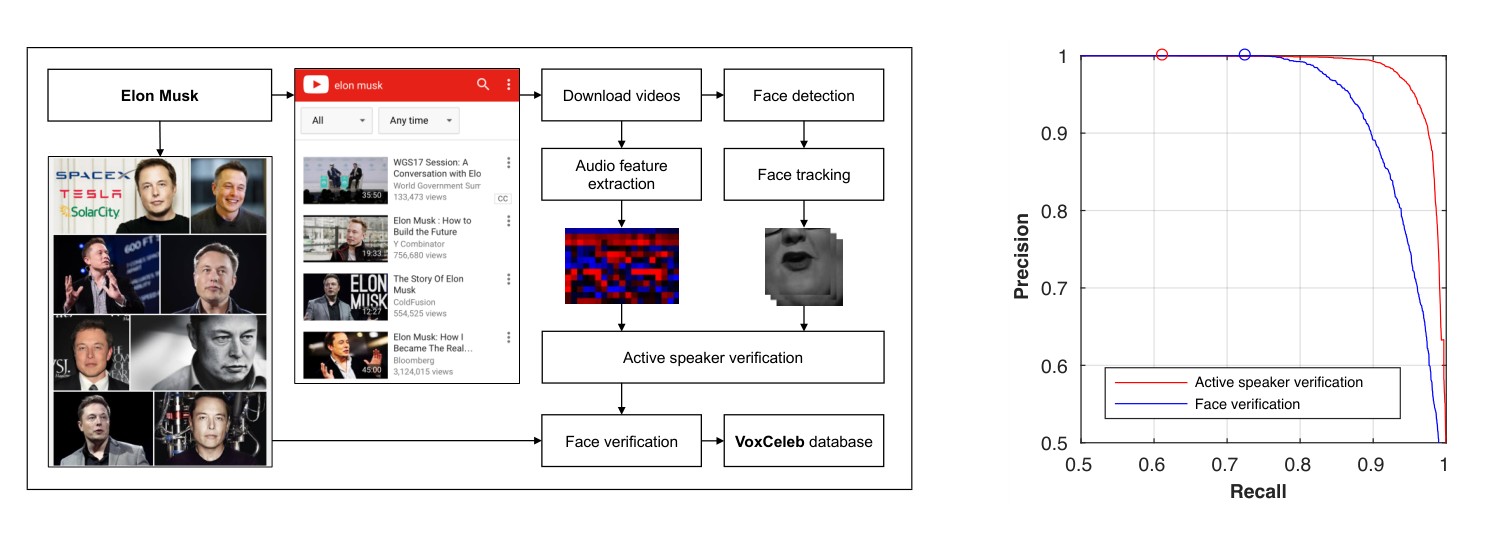
Figure 1: Left: Data processing pipeline; Right: Precision-recall curves for the active speaker verification (using a 25-frame window) and the face verification steps, tested on standard benchmark datasets [30, 31]. Operating points are shown in circles.
图 1:左:数据处理流水线;右:主动说话人核验(使用 25 帧窗口)和人脸验证步骤在标准基准数据集 [30, 31] 上的精度–召回曲线。工作点用圆圈标出。
Table 3: Precision-recall values at the chosen operating points.
| Task | Dataset | Precision | Recall |
|---|---|---|---|
| Active speaker verification | [31] | 1.000 | 0.613 |
| Face verification | [30] | 1.000 | 0.726 |
表 3:所选工作点上的精度–召回值。
| 任务 | 数据集 | 精度 | 召回率 |
|---|---|---|---|
| 主动说话人核验 | [31] | 1.000 | 0.613 |
| 人脸验证 | [30] | 1.000 | 0.726 |
- CNN Design and Architecture
- CNN 设计与架构
Our aim is to move from techniques that require traditional hand-crafted features, to a CNN architecture that can choose the features required for the task of speaker recognition. This allows us to minimise the pre-processing of the audio data and hence avoid losing valuable information in the process.
我们的目标是离开依赖传统手工特征的方法,走向一种能够自行选择说话人识别所需特征的 CNN 架构。这样可以把音频预处理降到最低,从而避免在处理过程中丢失有价值的信息。
Input features. All audio is first converted to single-channel, 16-bit streams at a 16kHz sampling rate for consistency. Spectrograms are then generated in a sliding window fashion using a hamming window of width 25ms, step 10ms and 1024-point FFT. This gives spectrograms of size 512 x 300 for 3 seconds of speech. Mean and variance normalisation is performed on every frequency bin of the spectrum. This normalisation is crucial, leading to an almost 10% increase in classification accuracy, as shown in Table 7. No other speech-specific pre-processing (e.g. silence removal, voice activity detection, or removal of unvoiced speech) is used. These short time magnitude spectrograms are then used as input to the CNN.
输入特征。 为保持一致,所有音频先转换成单通道、16 位、16kHz 采样率的数据流。随后用宽度 25ms、步长 10ms、1024 点 FFT 的汉明窗,以滑窗方式生成语谱图。这样,3 秒语音对应大小为 512 × 300 的语谱图。对频谱的每一个频率箱做均值和方差归一化。这一归一化至关重要,可使分类准确率提高近 10%,如表 7 所示。不再使用其他语音专用预处理(例如去静音、语音活动检测,或去掉清音)。这些短时幅度语谱图随后作为 CNN 的输入。
Architecture. Since speaker identification under a closed set can be treated as a multiple-class classification problem, we base our architecture on the VGG-M [37] CNN, known for good classification performance on image data, with modifications to adapt to the spectrogram input. The fully connected fc6 layer of dimension 9 × 8 (support in both dimensions) is replaced by two layers – a fully connected layer of 9 × 1 (support in the frequency domain) and an average pool layer with support 1 × n, where n depends on the length of the input speech segment (for example for a 3 second segment, n = 8). This makes the network invariant to temporal position but not frequency, and at the same time keeps the output dimensions the same as those of the original fully connected layer. This also reduces the number of parameters from 319M in VGG-M to 67M in our network, which helps avoid overfitting. The complete CNN architecture is specified in Table 4.
架构。 封闭集上的说话人识别可以看作多类分类问题,因此我们以在图像数据上分类表现良好的 VGG-M [37] CNN 为基础,并加以修改以适应语谱图输入。原来支撑为 9 × 8(两个方向都有支撑)的全连接层 fc6,被替换成两层:一个支撑为 9 × 1(仅在频率方向)的全连接层,以及一个支撑为 1 × n 的平均池化层,其中 n 取决于输入语音片段的长度(例如 3 秒片段时 n = 8)。这样网络对时间位置保持不变、对频率则不然,同时输出维度与原来的全连接层相同。参数量也从 VGG-M 的 3.19 亿降到我们网络中的 6700 万,有助于避免过拟合。完整的 CNN 架构见表 4。
Identification. Since identification is treated as a simple classification task, the output of the last layer is fed into a 1,251-way softmax in order to produce a distribution over the 1,251 different speakers.
识别。 由于识别被当作简单的分类任务,最后一层的输出会送入 1251 路 softmax,从而得到在 1251 位不同说话人上的分布。
Verification. For verification, feature vectors can be obtained from the classification network using the 1024 dimension fc7 vectors, and a cosine distance can be used to compare vectors. However, it is better to learn an embedding by training a Siamese network with a contrastive loss [38]. This is better suited to the verification task as the network learns to optimize similarity directly, rather than indirectly via a classification loss. For the embedding network, the last fully connected layer (fc8) is modified so that the output size is 256 instead of the number of classes. We compare both methods in the experiments.
验证。 做验证时,可以从分类网络取出 1024 维的 fc7 向量作为特征,再用余弦距离比较向量。不过,更好的做法是用对比损失 [38] 训练孪生网络来学习嵌入。这种方法更适合验证任务,因为网络直接优化相似度,而不是经由分类损失间接优化。对于嵌入网络,最后的全连接层(fc8)被改成输出 256 维,而不是类别数。我们在实验中对两种方法都做了比较。
Testing. A traditional approach to handling variable length utterances at test time is to break them up into fixed length segments (e.g. 3 seconds) and average the results on each segment to give a final class prediction. Average pooling, however allows the network to accommodate variable length inputs at test time, as the entire test utterance can be evaluated at once by changing the size of the apool6 layer. Not only is this more elegant, it also leads to an increase in classification accuracy, as shown in Table 7.
测试。 测试时处理变长话语的传统做法,是把它们切成固定长度的片段(例如 3 秒),再对各片段的结果取平均,得到最终类别预测。而平均池化使网络在测试时就能接受变长输入:只需改变 apool6 层的大小,整段测试话语便可一次评估完毕。这样做不仅更简洁,还能提高分类准确率,如表 7 所示。
Table 4: CNN architecture. The data size up to fc6 is for a 3-second input, but the network is able to accept inputs of variable lengths.
| Layer | Support | Filt dim. | # filts. | Stride | Data size |
|---|---|---|---|---|---|
| conv1 | 7×7 | 1 | 96 | 2×2 | 254×148 |
| mpool1 | 3×3 | - | - | 2×2 | 126×73 |
| conv2 | 5×5 | 96 | 256 | 2×2 | 62×36 |
| mpool2 | 3×3 | - | - | 2×2 | 30×17 |
| conv3 | 3×3 | 256 | 256 | 1×1 | 30×17 |
| conv4 | 3×3 | 256 | 256 | 1×1 | 30×17 |
| conv5 | 3×3 | 256 | 256 | 1×1 | 30×17 |
| mpool5 | 5×3 | - | - | 3×2 | 9×8 |
| fc6 | 9×1 | 256 | 4096 | 1×1 | 1×8 |
| apool6 | 1×n | - | - | 1×1 | 1×1 |
| fc7 | 1×1 | 4096 | 1024 | 1×1 | 1×1 |
| fc8 | 1×1 | 1024 | 1251 | 1×1 | 1×1 |
表 4:CNN 架构。直到 fc6 的数据尺寸对应 3 秒输入,但网络能够接受变长输入。
| 层 | 支撑 | 滤波器维数 | 滤波器数 | 步长 | 数据尺寸 |
|---|---|---|---|---|---|
| conv1 | 7×7 | 1 | 96 | 2×2 | 254×148 |
| mpool1 | 3×3 | - | - | 2×2 | 126×73 |
| conv2 | 5×5 | 96 | 256 | 2×2 | 62×36 |
| mpool2 | 3×3 | - | - | 2×2 | 30×17 |
| conv3 | 3×3 | 256 | 256 | 1×1 | 30×17 |
| conv4 | 3×3 | 256 | 256 | 1×1 | 30×17 |
| conv5 | 3×3 | 256 | 256 | 1×1 | 30×17 |
| mpool5 | 5×3 | - | - | 3×2 | 9×8 |
| fc6 | 9×1 | 256 | 4096 | 1×1 | 1×8 |
| apool6 | 1×n | - | - | 1×1 | 1×1 |
| fc7 | 1×1 | 4096 | 1024 | 1×1 | 1×1 |
| fc8 | 1×1 | 1024 | 1251 | 1×1 | 1×1 |
Implementation details and training. Our implementation is based on the deep learning toolbox MatConvNet [39] and trained on a NVIDIA TITAN X GPU. The network is trained using batch normalisation [40] and all hyper-parameters (e.g. weight decay, learning rates) use the default values provided with the toolbox. To reduce overfitting, we augment the data by taking random 3-second crops in the time domain during training. Using a fixed input length is also more efficient. For verification, the network is first trained for classification (excluding the test POIs for the verification task, see Section 6), and then all filter weights are frozen except for the modified last layer and the Siamese network trained with contrastive loss. Choosing good pairs for training is very important in metric learning. We randomly select half of the negative examples, and the other half using Hard Negative Mining, where we only sample from the hardest 10% of all negatives.
实现细节与训练。 我们的实现基于深度学习工具箱 MatConvNet [39],并在一块 NVIDIA TITAN X GPU 上训练。网络使用批归一化 [40] 训练,全部超参数(例如权重衰减、学习率)采用工具箱提供的默认值。为减少过拟合,训练时在时间维上随机裁出 3 秒片段做数据增强。使用固定输入长度也更高效。对于验证,网络先按分类任务训练(排除验证任务的测试目标人物,见第 6 节),随后除被修改的最后一层外冻住所有滤波权重,再用对比损失训练孪生网络。在度量学习中,选择合适的训练对非常重要。我们随机选取一半负例,另一半则用困难负例挖掘,只从全部负例中最难的 10% 里抽样。
- Experiments
- 实验
This section describes the experimental setup for both speaker identification and verification, and compares the performance of our devised CNN baseline to a number of traditional state of the art methods on VoxCeleb.
本节介绍说话人识别和验证的实验设置,并在 VoxCeleb 上把我们设计的 CNN 基线与若干传统的先进方法进行比较。
6.1. Experimental setup
6.1. 实验设置
Speaker identification. For identification, the training and the testing are performed on the same POIs. From each POI, we reserve the speech segments from one video for test. The test video contains at least 5 non-overlapping segments of speech. For identification, we report top-1 and top-5 accuracies. The statistics are given in Table 5.
说话人识别。 做识别时,训练和测试使用同一批目标人物。对每一位目标人物,我们留出其中一部视频里的语音片段作为测试。测试视频至少包含 5 段互不重叠的语音。识别任务报告 top-1 和 top-5 准确率。统计数字见表 5。
Speaker verification. For verification, all POIs whose name starts with an ‘E’ are reserved for testing, since this gives a good balance of male and female speakers. These POIs are not used for training the network, and are only used at test time. The statistics are given in Table 6.
说话人验证。 做验证时,所有姓名以字母 “E” 开头的目标人物被留作测试,因为这样可以得到较均衡的男女说话人。这些目标人物不用于训练网络,只在测试时使用。统计数字见表 6。
Two key performance metrics are used to evaluate system performance for the verification task. The metrics are similar to those used by existing datasets and challenges, such as NIST SRE12 [29] and SITW [5]. The primary metric is based on the cost function
验证任务使用两项关键指标来衡量系统表现。这些指标与现有数据集和评测(例如 NIST SRE12 [29] 和 SITW [5])所用的相近。主指标基于代价函数
where we assume a prior target probability of 0.01 and equal weights of 1.0 between misses and false alarms . The primary metric, , is the minimum value of for the range of thresholds. The alternative performance measure used here is the Equal Error Rate (EER) which is the rate at which both acceptance and rejection errors are equal. This measure is commonly used for identity verification systems.
其中我们假设目标先验概率 为 0.01,漏检 与虚警 的权重同为 1.0。主指标 是在阈值范围内 的最小值。这里使用的另一项指标是等错误率(EER),即接受错误与拒绝错误相等时的比率。该指标常用于身份验证系统。
Table 5: Development and test set statistics for identification.
| Set | # POIs | # Vid. / POI | # Utterances |
|---|---|---|---|
| Dev | 1,251 | 17.0 | 139,124 |
| Test | 1,251 | 1.0 | 6,255 |
表 5:识别任务的开发集和测试集统计。
| 集合 | 目标人物数 | 每人视频数 | 话语数 |
|---|---|---|---|
| Dev | 1,251 | 17.0 | 139,124 |
| Test | 1,251 | 1.0 | 6,255 |
Table 6: Development and test set statistics for verification.
| Set | # POIs | # Vid. / POI | # Utterances |
|---|---|---|---|
| Dev | 1,211 | 18.0 | 140,664 |
| Test | 40 | 17.4 | 4,715 |
表 6:验证任务的开发集和测试集统计。
| 集合 | 目标人物数 | 每人视频数 | 话语数 |
|---|---|---|---|
| Dev | 1,211 | 18.0 | 140,664 |
| Test | 40 | 17.4 | 4,715 |
6.2. Baselines
6.2. 基线
GMM-UBM. The GMM-UBM system uses MFCCs of dimension 13 as input. Cepstral mean and variance normalisation (CMVN) is applied on the features. Using the conventional GMM-UBM framework, a single speaker-independent universal background model (UBM) of 1024 mixture components is trained for 10 iterations from the training data.
GMM-UBM。 GMM-UBM 系统以 13 维 MFCC 为输入,并对特征做倒谱均值方差归一化(CMVN)。在常规 GMM-UBM 框架下,用训练数据训练一个含 1024 个混合成分、与说话人无关的通用背景模型(UBM),共迭代 10 次。
I-vectors/PLDA. Gender independent i-vector extractors [10] are trained on the VoxCeleb dataset to produce 400-dimensional i-vectors. Probabilistic LDA (PLDA) [41] is then used to reduce the dimension of the i-vectors to 200.
I-vector/PLDA。 在 VoxCeleb 数据集上训练与性别无关的 i-vector 提取器 [10],得到 400 维 i-vector。随后用概率 LDA(PLDA)[41] 把 i-vector 降到 200 维。
Inference. For identification, a one-vs-rest binary SVM classifier is trained for each speaker (). All feature inputs to the SVM are L2 normalised and a held out validation set is used to determine the C parameter (determines trade off between maximising the margin and penalising training errors). Classification during test time is done by choosing the speaker corresponding to the highest SVM score. The PLDA scoring function [41] is used for verification.
推断。 做识别时,为每一位说话人 ()训练一个一对多的二分类 SVM。送入 SVM 的全部特征都做 L2 归一化,并用留出的验证集确定 C 参数(该参数权衡最大化间隔与惩罚训练误差)。测试时选择 SVM 分数最高的那位说话人。验证则使用 PLDA 打分函数 [41]。
6.3. Results
6.3. 结果
Results are given in Tables 7 and 8. For both speaker recognition tasks, the CNN provides superior performance to the traditional state-of-the-art baselines.
结果见表 7 和表 8。在两项说话人识别任务上,CNN 的表现都优于传统的先进基线。
For identification we achieve an 80.5% top-1 classification accuracy over 1,251 different classes, almost 20% higher than traditional state of the art baselines. The CNN architecture uses the average pooling layer for variable length test data. We also compare to two variants: ‘CNN-fc-3s’, this architecture has a fully connected fc6 layer, and divides the test data into 3s segments and averages the scores. As is evident there is a considerable drop in performance compared to the average pooling original – partly due to the increased number of parameters that must be learnt; ‘CNN-fc-3s no var. norm.’, this is the CNN-fc-3s architecture without the variance normalization pre-processing of the input (the input is still mean normalized). The difference in performance between the two shows the importance of variance normalization for this data.
在识别任务上,我们在 1251 个不同类别上取得了 80.5% 的 top-1 分类准确率,比传统先进基线高出近 20 个百分点。该 CNN 架构使用平均池化层来处理变长测试数据。我们还比较了两个变体:“CNN-fc-3s” 使用全连接的 fc6 层,并把测试数据切成 3 秒片段再对分数取平均。可以看出,与采用平均池化的原网络相比,性能明显下降,部分原因是需要学习的参数变多了;“CNN-fc-3s no var. norm.” 则是去掉输入方差归一化预处理的 CNN-fc-3s(输入仍做均值归一化)。两者的性能差异说明,对这份数据来说方差归一化很重要。
For verification, the margin over the baselines is narrower, but still a significant improvement, with the embedding being the crucial step.
在验证任务上,相对基线的优势幅度更窄,但仍是显著提升,其中嵌入是关键一步。
Table 7: Results for identification on VoxCeleb (higher is better). The different CNN architectures are described in Section 5.
| Accuracy | Top-1 (%) | Top-5 (%) |
|---|---|---|
| I-vectors + SVM | 49.0 | 56.6 |
| I-vectors + PLDA + SVM | 60.8 | 75.6 |
| CNN-fc-3s no var. norm. | 63.5 | 80.3 |
| CNN-fc-3s | 72.4 | 87.4 |
| CNN | 80.5 | 92.1 |
表 7:VoxCeleb 上的识别结果(越高越好)。不同 CNN 架构见第 5 节。
| 方法 | Top-1(%) | Top-5(%) |
|---|---|---|
| I-vectors + SVM | 49.0 | 56.6 |
| I-vectors + PLDA + SVM | 60.8 | 75.6 |
| CNN-fc-3s no var. norm. | 63.5 | 80.3 |
| CNN-fc-3s | 72.4 | 87.4 |
| CNN | 80.5 | 92.1 |
Table 8: Results for verification on VoxCeleb (lower is better).
| Metrics | EER (%) | |
|---|---|---|
| GMM-UBM | 0.80 | 15.0 |
| I-vectors + PLDA | 0.73 | 8.8 |
| CNN-1024D | 0.75 | 10.2 |
| CNN-256D Embedding | 0.71 | 7.8 |
表 8:VoxCeleb 上的验证结果(越低越好)。
| 指标 | EER(%) | |
|---|---|---|
| GMM-UBM | 0.80 | 15.0 |
| I-vectors + PLDA | 0.73 | 8.8 |
| CNN-1024D | 0.75 | 10.2 |
| CNN-256D Embedding | 0.71 | 7.8 |
- Conclusions
- 结论
We provide a fully automated and scalable pipeline for audio data collection and use it to create a large-scale speaker identification dataset called VoxCeleb, with 1,251 speakers and over 100,000 utterances. In order to establish benchmark performance, we develop a novel CNN architecture with the ability to deal with variable length audio inputs, which outperforms traditional state-of-the-art methods for both speaker identification and verification on this dataset.
我们提供了一条完全自动、可扩展的音频数据收集流水线,并用它创建了名为 VoxCeleb 的大规模说话人识别数据集,包含 1251 位说话人和超过 10 万段话语。为建立基准表现,我们设计了一种能够处理变长音频输入的新 CNN 架构,它在该数据集上的说话人识别和验证都超过了传统的先进方法。
- Acknowledgements
- 致谢
Funding for this research is provided by the EPSRC Programme Grant Seebibyte EP/M013774/1 and IARPA grant JANUS. We would like to thank Andrew Senior for helpful comments.
本项研究由 EPSRC Programme Grant Seebibyte EP/M013774/1 以及 IARPA 的 JANUS 资助。感谢 Andrew Senior 提供的有益意见。
- References
- 参考文献
[1] L. L. Stoll, “Finding difficult speakers in automatic speaker recognition,” Technical Report No. UCB/EECS-2011-152, 2011.
[2] A. Krizhevsky, I. Sutskever, and G. E. Hinton, “ImageNet classification with deep convolutional neural networks,” in Advances in Neural Information Processing Systems, pp. 1106–1114, 2012.
[3] K. Simonyan and A. Zisserman, “Very deep convolutional networks for large-scale image recognition,” in Proceedings of the International Conference on Learning Representations, 2015.
[4] K. He, X. Zhang, S. Ren, and J. Sun, “Deep residual learning for image recognition,” arXiv preprint arXiv:1512.03385, 2015.
[5] M. McLaren, L. Ferrer, D. Castan, and A. Lawson, “The speakers in the wild (SITW) speaker recognition database,” INTERSPEECH, vol. 2016, 2016.
[6] O. Russakovsky, J. Deng, H. Su, J. Krause, S. Satheesh, S. Ma, S. Huang, A. Karpathy, A. Khosla, M. Bernstein, A. Berg, and F. Li, “Imagenet large scale visual recognition challenge,” International Journal of Computer Vision, 2015.
[7] D. A. Reynolds, T. F. Quatieri, and R. B. Dunn, “Speaker verification using adapted gaussian mixture models,” Digital signal processing, vol. 10, no. 1-3, pp. 19–41, 2000.
[8] D. A. Reynolds and R. C. Rose, “Robust text-independent speaker identification using gaussian mixture speaker models,” IEEE transactions on speech and audio processing, vol. 3, no. 1, pp. 72–83, 1995.
[9] P. Kenny, “Joint factor analysis of speaker and session variability: Theory and algorithms,” CRIM, Montreal, CRIM-06/08-13, 2005.
[10] N. Dehak, P. J. Kenny, R. Dehak, P. Dumouchel, and P. Ouellet, “Front-end factor analysis for speaker verification,” IEEE Transactions on Audio, Speech, and Language Processing, vol. 19, no. 4, pp. 788–798, 2011.
[11] U. H. Yapanel, X. Zhang, and J. H. Hansen, “High performance digit recognition in real car environments.,” in INTERSPEECH, 2002.
[12] J. H. Hansen, R. Sarikaya, U. H. Yapanel, and B. L. Pellom, “Robust speech recognition in noise: an evaluation using the spine corpus.,” in INTERSPEECH, pp. 905–908, 2001.
[13] T. N. Sainath, R. J. Weiss, A. W. Senior, K. W. Wilson, and O. Vinyals, “Learning the speech front-end with raw waveform CLDNNs,” in INTERSPEECH, pp. 1–5, 2015.
[14] S. Hershey, S. Chaudhuri, D. P. Ellis, J. F. Gemmeke, A. Jansen, R. C. Moore, M. Plakal, D. Platt, R. A. Saurous, B. Seybold, et al., “CNN architectures for large-scale audio classification,” arXiv preprint arXiv:1609.09430, 2016.
[15] Y. Lukic, C. Vogt, O. Dürr, and T. Stadelmann, “Speaker identification and clustering using convolutional neural networks,” in IEEE 26th International Workshop on Machine Learning for Signal Processing (MLSP), pp. 1–6, IEEE, 2016.
[16] D. van der Vloed, J. Bouten, and D. A. van Leeuwen, “NFI-FRITS: a forensic speaker recognition database and some first experiments,” in The Speaker and Language Recognition Workshop, 2014.
[17] J. Hennebert, H. Melin, D. Petrovska, and D. Genoud, “POLYCOST: a telephone-speech database for speaker recognition,” Speech communication, vol. 31, no. 2, pp. 265–270, 2000.
[18] J. B. Millar, J. P. Vonwiller, J. M. Harrington, and P. J. Dermody, “The Australian national database of spoken language,” in Proceedings of the IEEE International Conference on Acoustics, Speech and Signal Processing, vol. 1, pp. I–97, IEEE, 1994.
[19] J. S. Garofolo, L. F. Lamel, W. M. Fisher, J. G. Fiscus, and D. S. Pallett, “DARPA TIMIT acoustic-phonetic continous speech corpus CD-ROM. NIST speech disc 1-1.1,” NASA STI/Recon technical report, vol. 93, 1993.
[20] C. McCool and S. Marcel, “Mobio database for the ICPR 2010 face and speech competition,” tech. rep., IDIAP, 2009.
[21] R. Woo, A. Park, and T. J. Hazen, “The MIT Mobile Device Speaker Verification Corpus: Data collection and preliminary experiments,” The Speaker and Language Recognition Workshop, 2006.
[22] G. Morrison, C. Zhang, E. Enzinger, F. Ochoa, D. Bleach, M. Johnson, B. Folkes, S. De Souza, N. Cummins, and D. Chow, “Forensic database of voice recordings of 500+ Australian English speakers,” URL: http://databases.forensic-voice-comparison.net, 2015.
[23] A. Janin, D. Baron, J. Edwards, D. Ellis, D. Gelbart, N. Morgan, B. Peskin, T. Pfau, E. Shriberg, A. Stolcke, et al., “The ICSI meeting corpus,” in Proceedings of the IEEE International Conference on Acoustics, Speech and Signal Processing, vol. 1, IEEE, 2003.
[24] I. McCowan, J. Carletta, W. Kraaij, S. Ashby, S. Bourban, M. Flynn, M. Guillemot, T. Hain, J. Kadlec, V. Karaiskos, et al., “The AMI meeting corpus,” in International Conference on Methods and Techniques in Behavioral Research, vol. 88, 2005.
[25] P. Bell, M. J. Gales, T. Hain, J. Kilgour, P. Lanchantin, X. Liu, A. McParland, S. Renals, O. Saz, M. Wester, et al., “The MGB challenge: Evaluating multi-genre broadcast media recognition,” in IEEE Workshop on Automatic Speech Recognition and Understanding, pp. 687–693, IEEE, 2015.
[26] L. Feng and L. K. Hansen, “A new database for speaker recognition,” tech. rep., 2005.
[27] J. J. Godfrey, E. C. Holliman, and J. McDaniel, “Switchboard: Telephone speech corpus for research and development,” in Proceedings of the IEEE International Conference on Acoustics, Speech and Signal Processing, vol. 1, pp. 517–520, IEEE, 1992.
[28] W. M. Fisher, G. R. Doddington, and K. M. Goudie-Marshall, “The DARPA speech recognition research database: specifications and status,” in Proc. DARPA Workshop on speech recognition, pp. 93–99, 1986.
[29] C. S. Greenberg, “The NIST year 2012 speaker recognition evaluation plan,” NIST, Technical Report, 2012.
[30] O. M. Parkhi, A. Vedaldi, and A. Zisserman, “Deep face recognition,” in Proceedings of the British Machine Vision Conference, 2015.
[31] P. Chakravarty and T. Tuytelaars, “Cross-modal supervision for learning active speaker detection in video,” arXiv preprint arXiv:1603.08907, 2016.
[32] D. E. King, “Dlib-ml: A machine learning toolkit,” The Journal of Machine Learning Research, vol. 10, pp. 1755–1758, 2009.
[33] V. Kazemi and J. Sullivan, “One millisecond face alignment with an ensemble of regression trees,” in Proceedings of the IEEE Conference on Computer Vision and Pattern Recognition, pp. 1867–1874, 2014.
[34] J. S. Chung and A. Zisserman, “Lip reading in the wild,” in Proceedings of the Asian Conference on Computer Vision, 2016.
[35] M. Everingham, J. Sivic, and A. Zisserman, “Taking the bite out of automatic naming of characters in TV video,” Image and Vision Computing, vol. 27, no. 5, 2009.
[36] J. S. Chung and A. Zisserman, “Out of time: automated lip sync in the wild,” in Workshop on Multi-view Lip-reading, ACCV, 2016.
[37] K. Chatfield, K. Simonyan, A. Vedaldi, and A. Zisserman, “Return of the devil in the details: Delving deep into convolutional nets,” in Proceedings of the British Machine Vision Conference, 2014.
[38] S. Chopra, R. Hadsell, and Y. LeCun, “Learning a similarity metric discriminatively, with application to face verification,” in Proceedings of the IEEE Conference on Computer Vision and Pattern Recognition, vol. 1, pp. 539–546, IEEE, 2005.
[39] A. Vedaldi and K. Lenc, “Matconvnet – convolutional neural networks for MATLAB,” CoRR, vol. abs/1412.4564, 2014.
[40] S. Ioffe and C. Szegedy, “Batch normalization: Accelerating deep network training by reducing internal covariate shift,” arXiv preprint arXiv:1502.03167, 2015.
[41] S. Ioffe, “Probabilistic linear discriminant analysis,” in Proceedings of the European Conference on Computer Vision, pp. 531–542, Springer, 2006.