Supplementary Material of Conditional Variational Autoencoder with Adversarial Learning for End-to-End Text-to-Speech

条件变分自编码器与对抗学习的端到端文本转语音

Jaehyeon Kim Affiliation:  Kakao Enterprise, Seongnam-si, Gyeonggi-do, Republic of Korea Correspondence to: jay.xyz@kakaoenterprise.com    Jungil Kong Affiliation:  Kakao Enterprise, Seongnam-si, Gyeonggi-do, Republic of Korea    Juhee Son Affiliation:  Kakao Enterprise, Seongnam-si, Gyeonggi-do, Republic of Korea Affiliation:  School of Computing, KAIST, Daejeon, Republic of Korea

Abstract

摘要

Several recent end-to-end text-to-speech (TTS) models enabling single-stage training and parallel sampling have been proposed, but their sample quality does not match that of two-stage TTS systems. In this work, we present a parallel end-to-end TTS method that generates more natural sounding audio than current two-stage models. Our method adopts variational inference augmented with normalizing flows and an adversarial training process, which improves the expressive power of generative modeling. We also propose a stochastic duration predictor to synthesize speech with diverse rhythms from input text. With the uncertainty modeling over latent variables and the stochastic duration predictor, our method expresses the natural one-to-many relationship in which a text input can be spoken in multiple ways with different pitches and rhythms. A subjective human evaluation (mean opinion score, or MOS) on the LJ Speech, a single speaker dataset, shows that our method outperforms the best publicly available TTS systems and achieves a MOS comparable to ground truth.

近来已有若干支持单阶段训练与并行采样的端到端文本转语音（TTS）模型，但其样本质量仍不及两阶段 TTS 系统。本文提出一种并行端到端 TTS 方法，生成的音频自然度高于现有两阶段模型。该方法采用增强了归一化流与对抗训练过程的变分推断，以提升生成建模的表达能力。我们还提出随机时长预测器，使模型能从输入文本合成具有多样节奏的语音。借助对潜变量的不确定性建模与随机时长预测器，本方法能够表达「同一文本可用不同音高与节奏多种方式说出」这一自然的一对多关系。在单说话人数据集 LJ Speech 上的主观评测（平均意见分，MOS）表明，本方法超过当前最佳公开 TTS 系统，并达到与真值相当的 MOS。

1 Introduction

1 引言

Keywords:

Text-to-speech (TTS) systems synthesize raw speech waveforms from given text through several components. With the rapid development of deep neural networks, TTS system pipelines have been simplified to two-stage generative modeling apart from text preprocessing such as text normalization and phonemization. The first stage is to produce intermediate speech representations such as mel-spectrograms (Shen et al., 2018) or linguistic features (Oord et al., 2016) from the preprocessed text,[^1] and the second stage is to generate raw waveforms conditioned on the intermediate representations (Oord et al., 2016; Kalchbrenner et al., 2018). Models at each of the two-stage pipelines have been developed independently.

关键词：

文本转语音（TTS）系统通过若干组件，由给定文本合成原始语音波形。随着深度神经网络快速发展，除文本规范化与音素化等预处理外，TTS 流水线已简化为两阶段生成建模。第一阶段由预处理文本产生中间语音表示，例如梅尔频谱（Shen et al., 2018）或语言学特征（Oord et al., 2016）；[^1]第二阶段在中间表示条件下生成原始波形（Oord et al., 2016；Kalchbrenner et al., 2018）。两阶段流水线中的各模型彼此独立发展。

Neural network-based autoregressive TTS systems have shown the capability of synthesizing realistic speech (Shen et al., 2018; Li et al., 2019), but their sequential generative process makes it difficult to fully utilize modern parallel processors. To overcome this limitation and improve synthesis speed, several non-autoregressive methods have been proposed. In the text-to-spectrogram generation step, extracting attention maps from pre-trained autoregressive teacher networks (Ren et al., 2019; Peng et al., 2020) is attempted to decrease the difficulty of learning alignments between text and spectrograms. More recently, likelihood-based methods further eliminate the dependency on external aligners by estimating or learning alignments that maximize the likelihood of target mel-spectrograms (Zeng et al., 2020; Miao et al., 2020; Kim et al., 2020). Meanwhile, generative adversarial networks (GANs) (Goodfellow et al., 2014) have been explored in second stage models. GAN-based feed-forward networks with multiple discriminators, each distinguishing samples at different scales or periods, achieve high-quality raw waveform synthesis (Kumar et al., 2019; Bińkowski et al., 2019; Kong et al., 2020).

基于神经网络的自回归 TTS 系统已展现合成逼真语音的能力（Shen et al., 2018；Li et al., 2019），但其顺序生成过程难以充分利用现代并行处理器。为克服这一限制并提升合成速度，已有若干非自回归方法。在文本到频谱生成步骤中，有工作尝试从预训练自回归教师网络提取注意力图（Ren et al., 2019；Peng et al., 2020），以降低学习文本与频谱对齐的难度。更近的基于似然方法进一步通过估计或学习最大化目标梅尔频谱似然的对齐，消除对外部分对齐器的依赖（Zeng et al., 2020；Miao et al., 2020；Kim et al., 2020）。与此同时，生成对抗网络（GAN）（Goodfellow et al., 2014）在第二阶段模型中得到探索。带多个判别器、分别在不同尺度或周期上区分样本的 GAN 前馈网络，实现了高质量原始波形合成（Kumar et al., 2019；Bińkowski et al., 2019；Kong et al., 2020）。

Despite the progress of parallel TTS systems, two-stage pipelines remain problematic because they require sequential training or fine-tuning (Shen et al., 2018; Weiss et al., 2020) for high-quality production wherein latter stage models are trained with the generated samples of earlier stage models. In addition, their dependency on predefined intermediate features precludes applying learned hidden representations to obtain further improvements in performance. Recently, several works, i.e., FastSpeech 2s (Ren et al., 2021) and EATS (Donahue et al., 2021), have proposed efficient end-to-end training methods such as training over short audio clips rather than entire waveforms, leveraging a mel-spectrogram decoder to aid text representation learning, and designing a specialized spectrogram loss to relax length-mismatch between target and generated speech. However, despite potentially improving performance by utilizing the learned representations, their synthesis quality lags behind two-stage systems.

尽管并行 TTS 系统取得进展，两阶段流水线仍有问题：为达到高质量产品级效果，往往需要顺序训练或微调（Shen et al., 2018；Weiss et al., 2020），使后级模型在前级生成样本上训练。此外，对预定义中间特征的依赖，妨碍把学到的隐表示用于进一步提升表现。近来，FastSpeech 2s（Ren et al., 2021）与 EATS（Donahue et al., 2021）等工作提出高效端到端训练方法，例如在短音频片段而非整段波形上训练、借助梅尔频谱解码器辅助文本表示学习，以及设计专门的频谱损失以放松目标与生成语音之间的长度不匹配。然而，尽管利用学到的表示有望提升表现，其合成质量仍落后于两阶段系统。

In this work, we present a parallel end-to-end TTS method that generates more natural sounding audio than current two-stage models. Using a variational autoencoder (VAE) (Kingma & Welling, 2014), we connect two modules of TTS systems through latent variables to enable efficient end-to-end learning. To improve the expressive power of our method so that high-quality speech waveforms can be synthesized, we apply normalizing flows to our conditional prior distribution and adversarial training on the waveform domain. In addition to generating fine-grained audio, it is important for TTS systems to express the one-to-many relationship in which text input can be spoken in multiple ways with different variations (e.g., pitch and duration). To tackle the one-to-many problem, we also propose a stochastic duration predictor to synthesize speech with diverse rhythms from input text. With the uncertainty modeling over latent variables and the stochastic duration predictor, our method captures speech variations that cannot be represented by text.

本文提出一种并行端到端 TTS 方法，生成的音频自然度高于现有两阶段模型。我们用变分自编码器（VAE）（Kingma & Welling, 2014）通过潜变量连接 TTS 系统的两个模块，以实现高效端到端学习。为提升方法的表达能力以合成高质量语音波形，我们在条件先验分布上应用归一化流，并在波形域做对抗训练。除生成细粒度音频外，TTS 系统还需表达一对多关系：同一文本输入可用不同变化（如音高与时长）多种方式说出。为应对一对多问题，我们还提出随机时长预测器，以从输入文本合成多样节奏的语音。借助潜变量上的不确定性建模与随机时长预测器，本方法捕捉文本无法表示的语音变化。

Our method obtains more natural sounding speech and higher sampling efficiency than the best publicly available TTS system, Glow-TTS (Kim et al., 2020) with HiFi-GAN (Kong et al., 2020). We make both our demo page and source-code publicly available.[^2]

本方法获得的语音比当前最佳公开 TTS 系统 Glow-TTS（Kim et al., 2020）配合 HiFi-GAN（Kong et al., 2020）更自然，采样效率也更高。演示页与源码均已公开。[^2]

2 Method

2 方法

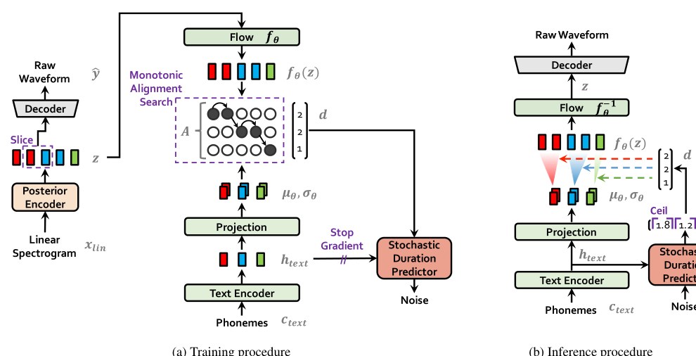
(a) Training procedure

（a）训练流程

In this section, we explain our proposed method and the architecture of it. The proposed method is mostly described in the first three subsections: a conditional VAE formulation; alignment estimation derived from variational inference; adversarial training for improving synthesis quality. The overall architecture is described at the end of this section. Figures 1(a) and 1(b) show the training and inference procedures of our method, respectively. From now on, we will refer to our method as Variational Inference with adversarial learning for end-to-end Text-to-Speech (VITS).

本节说明所提方法及其结构。方法主体在前三个小节：条件 VAE 表述；由变分推断导出的对齐估计；用于提升合成质量的对抗训练。整体结构在本节末描述。图 1(a) 与 1(b) 分别展示训练与推理流程。下文将本方法称为 Variational Inference with adversarial learning for end-to-end Text-to-Speech（VITS）。

2.1 Variational Inference

2.1 变分推断

2.1.1 Overview

VITS can be expressed as a conditional VAE with the objective of maximizing the variational lower bound, also called the evidence lower bound (ELBO), of the intractable marginal log-likelihood of data $\log{p_{\theta}(x|c)}$:

2.1.1 概述

VITS 可表述为条件 VAE，目标是最大化数据不可积边缘对数似然 $\log{p_{\theta}(x|c)}$ 的变分下界，亦称证据下界（ELBO）：

$$\log{p_{\theta}(x|c)}\geq\mathbb{E}_{q_{\phi}(z|x)}\Big[\log{p_{\theta}(x|z)}-\log{\frac{q_{\phi}(z|x)}{p_{\theta}(z|c)}}\Big] \tag{1}$$

where $p_{\theta}(z|c)$ denotes a prior distribution of the latent variables $z$ given condition $c$, $p_{\theta}(x|z)$ is the likelihood function of a data point $x$, and $q_{\phi}(z|x)$ is an approximate posterior distribution. The training loss is then the negative ELBO, which can be viewed as the sum of reconstruction loss $-\log{p_{\theta}(x|z)}$ and KL divergence $\log{q_{\phi}(z|x)}-\log{p_{\theta}(z|c)}$, where $z\sim q_{\phi}(z|x)$.

其中 $p_{\theta}(z|c)$ 表示给定条件 $c$ 时潜变量 $z$ 的先验，$p_{\theta}(x|z)$ 是数据点 $x$ 的似然，$q_{\phi}(z|x)$ 是近似后验。训练损失即为负 ELBO，可视为重建损失 $-\log{p_{\theta}(x|z)}$ 与 KL 散度 $\log{q_{\phi}(z|x)}-\log{p_{\theta}(z|c)}$ 之和，其中 $z\sim q_{\phi}(z|x)$。

2.1.2 Reconstruction loss

As a target data point in the reconstruction loss, we use a mel-spectrogram instead of a raw waveform, denoted by $x_{mel}$. We upsample the latent variables $z$ to the waveform domain $\hat{y}$ through a decoder and transform $\hat{y}$ to the mel-spectrogram domain $\hat{x}_{mel}$. Then the $L_{1}$ loss between the predicted and target mel-spectrogram is used as the reconstruction loss:

2.1.2 重建损失

重建损失中的目标数据点我们使用梅尔频谱而非原始波形，记为 $x_{mel}$。通过解码器将潜变量 $z$ 上采样到波形域 $\hat{y}$，再把 $\hat{y}$ 变换到梅尔频谱域 $\hat{x}_{mel}$。预测与目标梅尔频谱之间的 $L_{1}$ 损失即重建损失：

$$L_{recon}=\lVert x_{mel}-\hat{x}_{mel}\rVert_{1} \tag{2}$$

This can be viewed as maximum likelihood estimation assuming a Laplace distribution for the data distribution and ignoring constant terms. We define the reconstruction loss in the mel-spectrogram domain to improve the perceptual quality by using a mel-scale that approximates the response of the human auditory system. Note that the mel-spectrogram estimation from a raw waveform does not require trainable parameters as it only uses STFT and linear projection onto the mel-scale. Furthermore, the estimation is only employed during training, not inference. In practice, we do not upsample the whole latent variables $z$ but use partial sequences as an input for the decoder, which is the windowed generator training used for efficient end-to-end training (Ren et al., 2021; Donahue et al., 2021).

这可视为在假设数据分布为拉普拉斯分布并忽略常数项时的最大似然估计。我们在梅尔频谱域定义重建损失，以利用近似人耳响应的梅尔尺度提升感知质量。注意由原始波形估计梅尔频谱不需要可训练参数，仅用 STFT 与到梅尔尺度的线性投影。此外该估计只在训练时使用，推理不用。实践中我们不对整个潜变量 $z$ 上采样，而把部分序列作为解码器输入，即高效端到端训练中的窗口化生成器训练（Ren et al., 2021；Donahue et al., 2021）。

2.1.3 KL-divergence

The input condition of the prior encoder $c$ is composed of phonemes $c_{text}$ extracted from text and an alignment $A$ between phonemes and latent variables. The alignment is a hard monotonic attention matrix with $|c_{text}|\times|z|$ dimensions representing how long each input phoneme expands to be time-aligned with the target speech. Because there are no ground truth labels for the alignment, we must estimate the alignment at each training iteration, which we will discuss in Section 2.2.1. In our problem setting, we aim to provide more high-resolution information for the posterior encoder. We, therefore, use the linear-scale spectrogram of target speech $x_{lin}$ as input rather than the mel-spectrogram. Note that the modified input does not violate the properties of variational inference. The KL divergence is then:

2.1.3 KL 散度

先验编码器的输入条件 $c$ 由从文本提取的音素 $c_{text}$ 以及音素与潜变量之间的对齐 $A$ 组成。对齐是尺寸为 $|c_{text}|\times|z|$ 的硬单调注意力矩阵，表示每个输入音素扩展多长以与目标语音时间对齐。由于没有对齐的真值标签，必须在每次训练迭代中估计对齐，见第 2.2.1 节。在本问题设定下，我们希望为后验编码器提供更高分辨率信息，因此使用目标语音的线性尺度频谱 $x_{lin}$ 而非梅尔频谱作为输入。注意这一修改不违反变分推断的性质。KL 散度于是为：

$$\displaystyle L_{kl}=\log{q_{\phi}(z|x_{lin})}-\log{p_{\theta}(z|c_{text},A)}, \\ \displaystyle z\sim q_{\phi}(z|x_{lin})=N(z;\mu_{\phi}(x_{lin}),\sigma_{\phi}(x_{lin})) \tag{3}$$

The factorized normal distribution is used to parameterize our prior and posterior encoders. We found that increasing the expressiveness of the prior distribution is important for generating realistic samples. We, therefore, apply a normalizing flow $f_{\theta}$ (Rezende & Mohamed, 2015), which allows an invertible transformation of a simple distribution into a more complex distribution following the rule of change-of-variables, on top of the factorized normal prior distribution:

先验与后验编码器均用分解正态参数化。我们发现提升先验分布的表达能力对生成逼真样本很重要。因此在分解正态先验之上施加归一化流 $f_{\theta}$（Rezende & Mohamed, 2015），按变量替换法则把简单分布可逆变换为更复杂分布：

$$\displaystyle p_{\theta}(z|c) \\ \displaystyle=N(f_{\theta}(z);\mu_{\theta}(c),\sigma_{\theta}(c))\Big|\det\frac{\partial f_{\theta}(z)}{\partial z}\Big|, \\ \displaystyle c \\ \displaystyle=[c_{text},A] \tag{4}$$

2.2 Alignment Estimation

2.2 对齐估计

2.2.1 Monotonic alignment search

To estimate an alignment $A$ between input text and target speech, we adopt Monotonic Alignment Search (MAS) (Kim et al., 2020), a method to search an alignment that maximizes the likelihood of data parameterized by a normalizing flow $f$:

2.2.1 单调对齐搜索

为估计输入文本与目标语音之间的对齐 $A$，我们采用单调对齐搜索（MAS）（Kim et al., 2020）：搜索使由归一化流 $f$ 参数化的数据似然最大的对齐：

$$\displaystyle A \\ \displaystyle=\argmax\limits_{\hat{A}}\ {\log{p(x|c_{text},\hat{A})}} \\ \displaystyle=\argmax\limits_{\hat{A}}\ {\log{N(f(x);\mu(c_{text},\hat{A}),\sigma(c_{text},\hat{A}))}} \tag{5}$$

where the candidate alignments are restricted to be monotonic and non-skipping following the fact that humans read text in order without skipping any words. To find the optimum alignment, Kim et al. (2020) use dynamic programming. Applying MAS directly in our setting is difficult because our objective is the ELBO, not the exact log-likelihood. We, therefore, redefine MAS to find an alignment that maximizes the ELBO, which reduces to finding an alignment that maximizes the log-likelihood of the latent variables $z$:

其中候选对齐被限制为单调且不跳过，符合人按顺序朗读、不跳过词语的事实。为找最优对齐，Kim et al.（2020）使用动态规划。在我们的设定中直接应用 MAS 有困难，因为目标是 ELBO 而非精确对数似然。因此我们重新定义 MAS，使其寻找最大化 ELBO 的对齐，这归结为寻找最大化潜变量 $z$ 对数似然的对齐：

$$\displaystyle\argmax\limits_{\hat{A}}\ {\log{p_{\theta}(x_{mel}|z)}-\log{\frac{q_{\phi}(z|x_{lin})}{p_{\theta}(z|c_{text},\hat{A})}}} \\ \displaystyle=\argmax\limits_{\hat{A}}\ {\log{p_{\theta}(z|c_{text},\hat{A})}} \\ \displaystyle\;\;\;\;\;\;\;\;\;\;\;\;=\log{N(f_{\theta}(z);\mu_{\theta}(c_{text},\hat{A}),\sigma_{\theta}(c_{text},\hat{A}))} \tag{6}$$

Due to the resemblance of Equation 5 to Equation 6, we can use the original MAS implementation without modification. Appendix A includes pseudocode for MAS.

由于方程 5 与方程 6 形式相近，我们可以不加修改地使用原始 MAS 实现。附录 A 给出 MAS 伪代码。

2.2.2 Duration prediction from text

We can calculate the duration of each input token $d_{i}$ by summing all the columns in each row of the estimated alignment $\sum_{j}A_{i,j}$. The duration could be used to train a deterministic duration predictor, as proposed in previous work (Kim et al., 2020), but it cannot express the way a person utters at different speaking rates each time. To generate human-like rhythms of speech, we design a stochastic duration predictor so that its samples follow the duration distribution of given phonemes. The stochastic duration predictor is a flow-based generative model that is typically trained via maximum likelihood estimation. The direct application of maximum likelihood estimation, however, is difficult because the duration of each input phoneme is 1) a discrete integer, which needs to be dequantized for using continuous normalizing flows, and 2) a scalar, which prevents high-dimensional transformation due to invertibility. We apply variational dequantization (Ho et al., 2019) and variational data augmentation (Chen et al., 2020) to solve these problems. To be specific, we introduce two random variables $u$ and $\nu$, which have the same time resolution and dimension as that of the duration sequence $d$, for variational dequatization and variational data augmentation, respectively. We restrict the support of $u$ to be $[0,1)$ so that the difference $d-u$ becomes a sequence of positive real numbers, and we concatenate $\nu$ and $d$ channel-wise to make a higher dimensional latent representation. We sample the two variables through an approximate posterior distribution $q_{\phi}(u,\nu|d,c_{text})$. The resulting objective is a variational lower bound of the log-likelihood of the phoneme duration:

2.2.2 从文本预测时长

对估计对齐的每一行求和 $\sum_{j}A_{i,j}$，即可得到每个输入记号的时长 $d_{i}$。该时长可用于训练确定性时长预测器，如先前工作（Kim et al., 2020），但无法表达人每次以不同语速发音的方式。为生成类人的语音节奏，我们设计随机时长预测器，使其样本遵循给定音素的时长分布。随机时长预测器是基于流的生成模型，通常用最大似然估计训练。但直接做最大似然有困难：各输入音素的时长是 1）离散整数，需去量化才能用连续归一化流；2）标量，因可逆性限制而妨碍高维变换。我们用变分去量化（Ho et al., 2019）与变分数据增广（Chen et al., 2020）解决这些问题。具体地，引入与时长序列 $d$ 具有相同时间分辨率与维度的两个随机变量 $u$ 与 $\nu$，分别用于变分去量化与变分数据增广。将 $u$ 的支撑限制在 $[0,1)$，使差 $d-u$ 成为正实数序列，并将 $\nu$ 与 $d$ 沿通道拼接以得到更高维潜表示。通过近似后验 $q_{\phi}(u,\nu|d,c_{text})$ 采样这两个变量。所得目标是音素时长对数似然的变分下界：

$$\log{p_{\theta}(d|c_{text})}\geq\
\mathbb{E}{q{\phi}(u,\nu|d,c_{text})}\Big[\log{\frac{p_{\theta}(d-u,\nu|c_{text})}{q_{\phi}(u,\nu|d,c_{text})}}\Big] \tag{7}$$

The training loss $L_{dur}$ is then the negative variational lower bound. We apply the stop gradient operator (van den Oord et al., 2017), which prevents back-propagating the gradient of inputs, to the input conditions so that the training of the duration predictor does not affect that of other modules.

训练损失 $L_{dur}$ 即为负变分下界。我们对输入条件施加停止梯度算子（van den Oord et al., 2017），阻止输入梯度回传，使时长预测器的训练不影响其他模块。

The sampling procedure is relatively simple; the phoneme duration is sampled from random noise through the inverse transformation of the stochastic duration predictor, and then it is converted to integers.

采样过程相对简单：通过随机时长预测器的逆变换从随机噪声采样音素时长，再转换为整数。

2.3 Adversarial Training

2.3 对抗训练

To adopt adversarial training in our learning system, we add a discriminator $D$ that distinguishes between the output generated by the decoder $G$ and the ground truth waveform $y$. In this work, we use two types of loss successfully applied in speech synthesis; the least-squares loss function (Mao et al., 2017) for adversarial training, and the additional feature-matching loss (Larsen et al., 2016) for training the generator:

为在学习系统中引入对抗训练，我们加入判别器 $D$，以区分解码器 $G$ 的输出与真值波形 $y$。本文使用在语音合成中成功应用的两类损失：对抗训练的最小二乘损失（Mao et al., 2017），以及训练生成器时额外的特征匹配损失（Larsen et al., 2016）：

$$\displaystyle L_{adv}(D) \\ \displaystyle=\mathbb{E}_{(y,z)}\Big[(D(y)-1)^{2}+(D(G(z)))^{2}\Big], \\ \displaystyle L_{adv}(G) \\ \displaystyle=\mathbb{E}_{z}\Big[(D(G(z))-1)^{2}\Big], \\ \displaystyle L_{fm}(G) \\ \displaystyle=\mathbb{E}_{(y,z)}\Big[\sum_{l=1}^{T}\frac{1}{N_{l}}\lVert D^{l}(y)-D^{l}(G(z))\rVert_{1}\Big] \tag{8}$$

where $T$ denotes the total number of layers in the discriminator and $D^{l}$ outputs the feature map of the $l$-th layer of the discriminator with $N_{l}$ number of features. Notably, the feature matching loss can be seen as reconstruction loss that is measured in the hidden layers of the discriminator suggested as an alternative to the element-wise reconstruction loss of VAEs (Larsen et al., 2016).

其中 $T$ 为判别器总层数，$D^{l}$ 输出判别器第 $l$ 层特征图，特征数为 $N_{l}$。值得注意的是，特征匹配损失可视为在判别器隐层中度量的重建损失，被建议作为 VAE 逐元素重建损失的替代（Larsen et al., 2016）。

2.4 Final Loss

2.4 最终损失

With the combination of VAE and GAN training, the total loss for training our conditional VAE can be expressed as follows:

结合 VAE 与 GAN 训练，我们条件 VAE 的总训练损失可写为：

$$L_{vae}=L_{recon}+L_{kl}+L_{dur}+L_{adv}(G)+L_{fm}(G) \tag{11}$$

2.5 Model Architecture

2.5 模型结构

The overall architecture of the proposed model consists of a posterior encoder, prior encoder, decoder, discriminator, and stochastic duration predictor. The posterior encoder and discriminator are only used for training, not for inference. Architectural details are available in Appendix B.

所提模型整体由后验编码器、先验编码器、解码器、判别器与随机时长预测器组成。后验编码器与判别器仅用于训练、不用于推理。结构细节见附录 B。

2.5.1 Posterior Encoder

For the posterior encoder, we use the non-causal WaveNet residual blocks used in WaveGlow (Prenger et al., 2019) and Glow-TTS (Kim et al., 2020). A WaveNet residual block consists of layers of dilated convolutions with a gated activation unit and skip connection. The linear projection layer above the blocks produces the mean and variance of the normal posterior distribution. For the multi-speaker case, we use global conditioning (Oord et al., 2016) in residual blocks to add speaker embedding.

2.5.1 后验编码器

后验编码器使用 WaveGlow（Prenger et al., 2019）与 Glow-TTS（Kim et al., 2020）中的非因果 WaveNet 残差块。WaveNet 残差块由带门控激活与跳跃连接的膨胀卷积层组成。块上方的线性投影层产出正态后验分布的均值与方差。多说话人情形下，我们在残差块中用全局条件（Oord et al., 2016）加入说话人嵌入。

2.5.2 Prior Encoder

The prior encoder consists of a text encoder that processes the input phonemes $c_{text}$ and a normalizing flow $f_{\theta}$ that improves the flexibility of the prior distribution. The text encoder is a transformer encoder (Vaswani et al., 2017) that uses relative positional representation (Shaw et al., 2018) instead of absolute positional encoding. We can obtain the hidden representation $h_{text}$ from $c_{text}$ through the text encoder and a linear projection layer above the text encoder that produces the mean and variance used for constructing the prior distribution. The normalizing flow is a stack of affine coupling layers (Dinh et al., 2017) consisting of a stack of WaveNet residual blocks. For simplicity, we design the normalizing flow to be a volume-preserving transformation with the Jacobian determinant of one. For the multi-speaker setting, we add speaker embedding to the residual blocks in the normalizing flow through global conditioning.

2.5.2 先验编码器

先验编码器由处理输入音素 $c_{text}$ 的文本编码器，以及提升先验分布灵活性的归一化流 $f_{\theta}$ 组成。文本编码器是使用相对位置表示（Shaw et al., 2018）而非绝对位置编码的 Transformer 编码器（Vaswani et al., 2017）。通过文本编码器及其上方用于构造先验分布均值与方差的线性投影层，可由 $c_{text}$ 得到隐表示 $h_{text}$。归一化流是由 WaveNet 残差块堆叠构成的仿射耦合层堆叠（Dinh et al., 2017）。为简单起见，我们将归一化流设计为雅可比行列式为 1 的保体积变换。多说话人设定下，通过全局条件把说话人嵌入加入归一化流中的残差块。

2.5.3 Decoder

The decoder is essentially the HiFi-GAN V1 generator (Kong et al., 2020). It is composed of a stack of transposed convolutions, each of which is followed by a multi-receptive field fusion module (MRF). The output of the MRF is the sum of the output of residual blocks that have different receptive field sizes. For the multi-speaker setting, we add a linear layer that transforms speaker embedding and add it to the input latent variables $z$.

2.5.3 解码器

解码器本质上是 HiFi-GAN V1 生成器（Kong et al., 2020）。它由转置卷积堆叠组成，每个转置卷积后接多感受野融合模块（MRF）。MRF 的输出是具有不同感受野大小的残差块输出之和。多说话人设定下，我们加入线性层变换说话人嵌入，再加到输入潜变量 $z$ 上。

2.5.4 Discriminator

We follow the discriminator architecture of the multi-period discriminator proposed in HiFi-GAN (Kong et al., 2020). The multi-period discriminator is a mixture of Markovian window-based sub-discriminators (Kumar et al., 2019), each of which operates on different periodic patterns of input waveforms.

2.5.4 判别器

我们遵循 HiFi-GAN（Kong et al., 2020）提出的多周期判别器结构。多周期判别器是若干基于马尔可夫窗的子判别器的混合（Kumar et al., 2019），各自作用于输入波形的不同周期模式。

2.5.5 Stochastic Duration Predictor

The stochastic duration predictor estimates the distribution of phoneme duration from a conditional input $h_{text}$. For the efficient parameterization of the stochastic duration predictor, we stack residual blocks with dilated and depth-separable convolutional layers. We also apply neural spline flows (Durkan et al., 2019), which take the form of invertible nonlinear transformations by using monotonic rational-quadratic splines, to coupling layers. Neural spline flows improve transformation expressiveness with a similar number of parameters compared to commonly used affine coupling layers. For the multi-speaker setting, we add a linear layer that transforms speaker embedding and add it to the input $h_{text}$.

2.5.5 随机时长预测器

随机时长预测器由条件输入 $h_{text}$ 估计音素时长分布。为高效参数化，我们堆叠带膨胀与深度可分卷积层的残差块。耦合层还应用神经样条流（Durkan et al., 2019）：借助单调有理二次样条实现可逆非线性变换。相对常用仿射耦合层，神经样条流以相近参数量提升变换表达能力。多说话人设定下，加入线性层变换说话人嵌入并加到输入 $h_{text}$ 上。

3 Experiments

3 实验

3.1 Datasets

3.1 数据集

We conducted experiments on two different datasets. We used the LJ Speech dataset (Ito, 2017) for comparison with other publicly available models and the VCTK dataset (Veaux et al., 2017) to verify whether our model can learn and express diverse speech characteristics. The LJ Speech dataset consists of 13,100 short audio clips of a single speaker with a total length of approximately 24 hours. The audio format is 16-bit PCM with a sample rate of 22 kHz, and we used it without any manipulation. We randomly split the dataset into a training set (12,500 samples), validation set (100 samples), and test set (500 samples). The VCTK dataset consists of approximately 44,000 short audio clips uttered by 109 native English speakers with various accents. The total length of the audio clips is approximately 44 hours. The audio format is 16-bit PCM with a sample rate of 44 kHz. We reduced the sample rate to 22 kHz. We randomly split the dataset into a training set (43,470 samples), validation set (100 samples), and test set (500 samples).

我们在两个数据集上实验。用 LJ Speech（Ito, 2017）与其他公开模型比较，用 VCTK（Veaux et al., 2017）验证模型能否学习并表达多样语音特征。LJ Speech 含单说话人约 13,100 段短音频，总长约 24 小时；音频为 16 位 PCM、采样率 22 kHz，我们未做额外处理。随机划分为训练集（12,500）、验证集（100）与测试集（500）。VCTK 含约 109 位带不同口音的英语母语者所发约 44,000 段短音频，总长约 44 小时；原为 16 位 PCM、44 kHz，我们降采样到 22 kHz。随机划分为训练集（43,470）、验证集（100）与测试集（500）。

3.2 Preprocessing

3.2 预处理

We use linear spectrograms which can be obtained from raw waveforms through the Short-time Fourier transform (STFT), as input of the posterior encoder. The FFT size, window size and hop size of the transform are set to 1024, 1024 and 256, respectively. We use 80 bands mel-scale spectrograms for reconstruction loss, which is obtained by applying a mel-filterbank to linear spectrograms.

后验编码器输入使用可由原始波形经短时傅里叶变换（STFT）得到的线性频谱。变换的 FFT 大小、窗长与 hop 分别设为 1024、1024 与 256。重建损失使用 80 维梅尔频谱，由对线性频谱施加梅尔滤波器组得到。

We use International Phonetic Alphabet (IPA) sequences as input to the prior encoder. We convert text sequences to IPA phoneme sequences using open-source software (Bernard, 2021), and the converted sequences are interspersed with a blank token following the implementation of Glow-TTS.

先验编码器输入使用国际音标（IPA）序列。用开源软件（Bernard, 2021）把文本转为 IPA 音素序列，并按 Glow-TTS 实现在转换序列中插入空白记号。

3.3 Training

3.3 训练

The networks are trained using the AdamW optimizer (Loshchilov & Hutter, 2019) with $\beta_{1}=0.8$, $\beta_{2}=0.99$ and weight decay $\lambda=0.01$. The learning rate decay is scheduled by a $0.999^{1/8}$ factor in every epoch with an initial learning rate of $2\times 10^{-4}$. Following previous work (Ren et al., 2021; Donahue et al., 2021), we adopt the windowed generator training, a method of generating only a part of raw waveforms to reduce the training time and memory usage during training. We randomly extract segments of latent representations with a window size of 32 to feed to the decoder instead of feeding entire latent representations and also extract the corresponding audio segments from the ground truth raw waveforms as training targets. We use mixed precision training on 4 NVIDIA V100 GPUs. The batch size is set to 64 per GPU and the model is trained up to 800k steps.

网络用 AdamW 优化器（Loshchilov & Hutter, 2019）训练，$\beta_{1}=0.8$、$\beta_{2}=0.99$，权重衰减 $\lambda=0.01$。学习率按每 epoch 因子 $0.999^{1/8}$ 衰减，初始学习率为 $2\times 10^{-4}$。沿用先前工作（Ren et al., 2021；Donahue et al., 2021），采用窗口化生成器训练：只生成部分原始波形以减少训练时间与显存。我们随机抽取窗长为 32 的潜表示片段送入解码器，而非整段潜表示，并抽取对应真值波形片段作为训练目标。在 4 块 NVIDIA V100 GPU 上做混合精度训练，每 GPU 批大小 64，训练至 80 万步。

3.4 Experimental Setup for Comparison

3.4 比较实验设置

We compared our model with the best publicly available models. We used Tacotron 2, an autoregressive model, and Glow-TTS, a flow-based non-autoregressive model, as first stage models and HiFi-GAN as a second stage model. We used their public implementations and pre-trained weights.[^3] Since a two-stage TTS system can theoretically achieve higher synthesis quality through sequential training, we included the fine-tuned HiFi-GAN up to 100k steps with the predicted outputs from the first stage models. We empirically found that fine-tuning HiFi-GAN with the generated mel-spectrograms from Tacotron 2 under teacher-forcing mode, led to better quality for both Tacotron 2 and Glow-TTS than fine-tuning with the generated mel-spectrograms from Glow-TTS, so we appended the better fine-tuned HiFi-GAN to both Tacotron 2 and Glow-TTS.

我们与当前最佳公开模型比较。第一阶段用自回归的 Tacotron 2 与基于流的非自回归 Glow-TTS，第二阶段用 HiFi-GAN；均使用其公开实现与预训练权重。[^3]由于两阶段 TTS 理论上可通过顺序训练获得更高合成质量，我们还包含用第一阶段预测输出对 HiFi-GAN 微调至 10 万步的设置。经验上发现，用教师强制模式下 Tacotron 2 生成的梅尔频谱微调 HiFi-GAN，对 Tacotron 2 与 Glow-TTS 的质量都优于用 Glow-TTS 生成梅尔频谱微调，因此把该更好的微调 HiFi-GAN 同时接到 Tacotron 2 与 Glow-TTS。

As each model has a degree of randomness during sampling, we fixed hyper-parameters that controls the randomness of each model throughout our experiments. The probability of dropout in the pre-net of Tactron 2 was set to 0.5. For Glow-TTS, the standard deviation of the prior distribution was set to 0.333. For VITS, the standard deviation of input noise of the stochastic duration predictor was set to 0.8 and we multiplied a scale factor of 0.667 to the standard deviation of the prior distribution.

由于各模型采样时都有一定随机性，实验中固定控制随机性的超参。Tacotron 2 预网络 dropout 概率设为 0.5。Glow-TTS 先验分布标准差设为 0.333。VITS 随机时长预测器输入噪声标准差设为 0.8，并对先验分布标准差乘以尺度因子 0.667。

4 Results

4 结果

4.1 Speech Synthesis Quality

4.1 语音合成质量

We conducted crowd-sourced MOS tests to evaluate the quality. Raters listened to randomly selected audio samples, and rated their naturalness on a 5 point scale from 1 to 5. Raters were allowed to evaluate each audio sample once, and we normalized all the audio clips to avoid the effect of amplitude differences on the score. All of the quality assessments in this work were conducted in this manner.

我们进行众包 MOS 测试评估质量。评分者收听随机选取的音频样本，按 1 到 5 的五分制评价自然度。每个音频样本每位评分者只评一次；所有音频片段均做归一化，以避免幅度差异影响分数。本文所有质量评估均按此方式进行。

The evaluation results are shown in Table 1. VITS outperforms other TTS systems and achieves a similar MOS to that of ground truth. The VITS (DDP), which employs the same deterministic duration predictor architecture used in Glow-TTS rather than the stochastic duration predictor, scores the second-highest among TTS systems in the MOS evaluation. These results imply that 1) the stochastic duration predictor generates more realistic phoneme duration than the deterministic duration predictor and 2) our end-to-end training method is an effective way to make better samples than other TTS models even if maintaining the similar duration predictor architecture.

评测结果见表 1。VITS 超过其他 TTS 系统，并达到与真值相近的 MOS。采用与 Glow-TTS 相同确定性时长预测器结构、而非随机时长预测器的 VITS（DDP）在 MOS 中位列 TTS 系统第二。这些结果意味着：1）随机时长预测器生成的音素时长比确定性时长预测器更真实；2）即便保持相近的时长预测器结构，我们的端到端训练方法仍能有效生成优于其他 TTS 模型的样本。

Model	MOS (CI)
Ground Truth	4.46 ($\pm$0.06)
Tacotron 2 + HiFi-GAN	3.77 ($\pm$0.08)
Tacotron 2 + HiFi-GAN (Fine-tuned)	4.25 ($\pm$0.07)
Glow-TTS + HiFi-GAN	4.14 ($\pm$0.07)
Glow-TTS + HiFi-GAN (Fine-tuned)	4.32 ($\pm$0.07)
VITS (DDP)	4.39 ($\pm$0.06)
VITS	4.43 ($\pm$0.06)

Table 1: Comparison of evaluated MOS with 95% confidence intervals on the LJ Speech dataset.

模型	MOS（置信区间）
真值	4.46 ($\pm$0.06)
Tacotron 2 + HiFi-GAN	3.77 ($\pm$0.08)
Tacotron 2 + HiFi-GAN（微调）	4.25 ($\pm$0.07)
Glow-TTS + HiFi-GAN	4.14 ($\pm$0.07)
Glow-TTS + HiFi-GAN（微调）	4.32 ($\pm$0.07)
VITS（DDP）	4.39 ($\pm$0.06)
VITS	4.43 ($\pm$0.06)

表 1：LJ Speech 数据集上带 95% 置信区间的 MOS 比较。

We conducted an ablation study to demonstrate the effectiveness of our methods, including the normalized flow in the prior encoder and linear-scale spectrogram posterior input. All models in the ablation study were trained up to 300k steps. The results are shown in Table 2. Removing the normalizing flow in the prior encoder results in a 1.52 MOS decrease from the baseline, demonstrating that the prior distribution’s flexibility significantly influences the synthesis quality. Replacing the linear-scale spectrogram for posterior input with the mel-spectrogram results in a quality degradation (-0.19 MOS), indicating that the high-resolution information is effective for VITS in improving the synthesis quality.

我们做消融以验证方法有效性，包括先验编码器中的归一化流以及线性尺度频谱后验输入。消融中所有模型训练至 30 万步。结果见表 2。去掉先验编码器中的归一化流使 MOS 相对基线下降 1.52，说明先验分布灵活性显著影响合成质量。把后验输入的线性频谱换成梅尔频谱导致质量下降（-0.19 MOS），表明高分辨率信息有助于 VITS 提升合成质量。

Model	MOS (CI)
Ground Truth	4.50 ($\pm$0.06)
Baseline	4.50 ($\pm$0.06)
without Normalizing Flow	2.98 ($\pm$0.08)
with Mel-spectrogram	4.31 ($\pm$0.08)

Table 2: MOS comparison in the ablation studies.

模型	MOS（置信区间）
真值	4.50 ($\pm$0.06)
基线	4.50 ($\pm$0.06)
无归一化流	2.98 ($\pm$0.08)
用梅尔频谱	4.31 ($\pm$0.08)

表 2：消融研究中的 MOS 比较。

4.2 Generalization to Multi-Speaker Text-to-Speech

4.2 泛化到多说话人文本转语音

To verify that our model can learn and express diverse speech characteristics, we compared our model to Tacotron 2, Glow-TTS and HiFi-GAN, which showed the ability to extend to multi-speaker speech synthesis (Jia et al., 2018; Kim et al., 2020; Kong et al., 2020). We trained the models on the VCTK dataset. We added speaker embedding to our model as described in Section 2.5. For Tacotron 2, we broadcasted speaker embedding and concatenated it with the encoder output, and for Glow-TTS, we applied the global conditioning following the previous work. The evaluation method is the same as that described in Section 4.1. As shown in Table 3, our model achieves a higher MOS than the other models. This demonstrates that our model learns and expresses various speech characteristics in an end-to-end manner.

为验证模型能否学习并表达多样语音特征，我们与已展示可扩展到多说话人语音合成的 Tacotron 2、Glow-TTS 与 HiFi-GAN 比较（Jia et al., 2018；Kim et al., 2020；Kong et al., 2020）。模型在 VCTK 上训练。按第 2.5 节所述向本模型加入说话人嵌入；对 Tacotron 2，将说话人嵌入广播并与编码器输出拼接；对 Glow-TTS，按先前工作做全局条件。评估方式同第 4.1 节。如表 3 所示，本模型 MOS 高于其他模型，表明能以端到端方式学习并表达多种语音特征。

Model	MOS (CI)
Ground Truth	4.38 ($\pm$0.07)
Tacotron 2 + HiFi-GAN	3.14 ($\pm$0.09)
Tacotron 2 + HiFi-GAN (Fine-tuned)	3.19 ($\pm$0.09)
Glow-TTS + HiFi-GAN	3.76 ($\pm$0.07)
Glow-TTS + HiFi-GAN (Fine-tuned)	3.82 ($\pm$0.07)
VITS	4.38 ($\pm$0.06)

Table 3: Comparison of evaluated MOS with 95% confidence intervals on the VCTK dataset.

模型	MOS（置信区间）
真值	4.38 ($\pm$0.07)
Tacotron 2 + HiFi-GAN	3.14 ($\pm$0.09)
Tacotron 2 + HiFi-GAN（微调）	3.19 ($\pm$0.09)
Glow-TTS + HiFi-GAN	3.76 ($\pm$0.07)
Glow-TTS + HiFi-GAN（微调）	3.82 ($\pm$0.07)
VITS	4.38 ($\pm$0.06)

表 3：VCTK 数据集上带 95% 置信区间的 MOS 比较。

4.3 Speech Variation

4.3 语音多样性

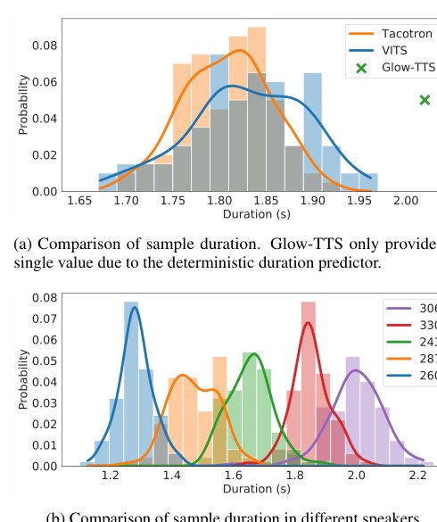
(a) Comparison of sample duration. Glow-TTS only provides a single value due to the deterministic duration predictor.

（a）样本时长比较。Glow-TTS 因确定性时长预测器只给出单一取值。

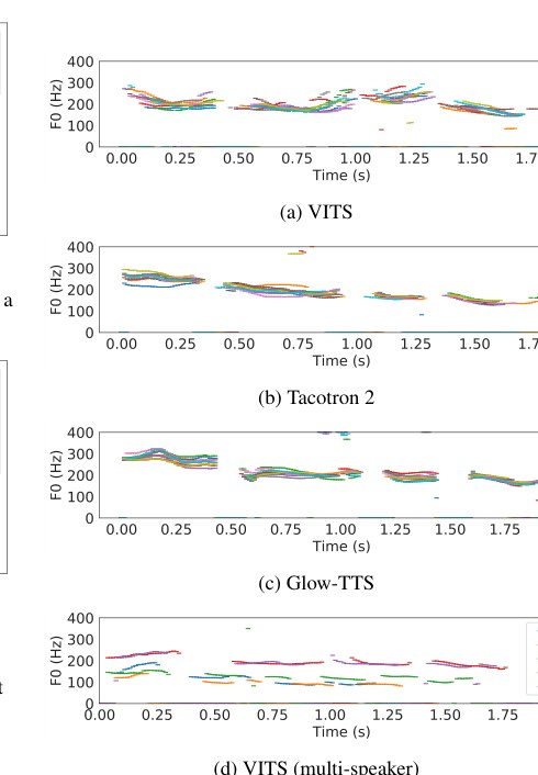
(a) VITS

（a）VITS

We verified how many different lengths of speech the stochastic duration predictor produces, and how many different speech characteristics the synthesized samples have. Similar to Valle et al. (2021), all samples here were generated from a sentence “How much variation is there?”. Figure 2(a) shows histograms of the lengths of 100 generated utterances from each model. While Glow-TTS generates only fixed-length utterances due to the deterministic duration predictor, samples from our model follow a similar length distribution to that of Tacotron 2. Figure 2(b) shows the lengths of 100 utterances generated with each of five speaker identities from our model in the multi-speaker setting, implying that the model learns the speaker-dependent phoneme duration. F0 contours of 10 utterances extracted with the YIN algorithm (De Cheveigné & Kawahara, 2002) in Figure 3 shows that our model generates speech with diverse pitches and rhythms, and five samples generated with each of different speaker identities in Figure 3(d) demonstrates our model expresses very different lengths and pitches of speech for each speaker identity. Note that Glow-TTS could increase the diversity of pitch by increasing the standard deviation of the prior distribution, but on the contrary, it could lower the synthesis quality.

我们检验随机时长预测器能产生多少种不同语音长度，以及合成样本具有多少不同语音特征。与 Valle et al.（2021）类似，此处所有样本均由句子 “How much variation is there?” 生成。图 2(a) 给出各模型 100 条生成话语的长度直方图。Glow-TTS 因确定性时长预测器只能生成固定长度话语，而本模型样本的长度分布与 Tacotron 2 相近。图 2(b) 给出多说话人设定下本模型对五个说话人身份各生成 100 条话语的长度，说明模型学到了依赖说话人的音素时长。图 3 用 YIN 算法（De Cheveigné & Kawahara, 2002）提取的 10 条话语 F0 轮廓显示，本模型能生成音高与节奏多样的语音；图 3(d) 中每个不同说话人身份各五条样本表明，模型能为各说话人身份表达差异很大的时长与音高。需注意，Glow-TTS 可通过增大先验分布标准差提高音高多样性，但反而可能降低合成质量。

4.4 Synthesis Speed

4.4 合成速度

We compared the synthesis speed of our model with a parallel two-stage TTS system, Glow-TTS and HiFi-GAN. We measured the synchronized elapsed time over the entire process to generate raw waveforms from phoneme sequences with 100 sentences randomly selected from the test set of the LJ Speech dataset. We used a single NVIDIA V100 GPU with a batch size of 1. The results are shown in Table 4. Since our model does not require modules for generating predefined intermediate representations, its sampling efficiency and speed are greatly improved.

我们将本模型的合成速度与并行两阶段 TTS 系统 Glow-TTS 与 HiFi-GAN 比较。在单块 NVIDIA V100、批大小为 1 的设置下，用从 LJ Speech 测试集随机抽取的 100 句，测量从音素序列生成原始波形全过程的同步耗时。结果见表 4。由于本模型无需用于生成预定义中间表示的模块，采样效率与速度大幅提升。

Model	Speed (kHz)	Real-time
Glow-TTS + HiFi-GAN	606.05	$\times$27.48
VITS	1480.15	$\times$67.12
VITS (DDP)	2005.03	$\times$90.93

Table 4: Comparison of the synthesis speed. Speed of $n$ kHz means that the model can generate $n\times 1000$ raw audio samples per second. Real-time means the synthesis speed over real-time.

模型	速度（kHz）	实时倍率
Glow-TTS + HiFi-GAN	606.05	$\times$27.48
VITS	1480.15	$\times$67.12
VITS（DDP）	2005.03	$\times$90.93

表 4：合成速度比较。速度 $n$ kHz 表示模型每秒可生成 $n\times 1000$ 个原始音频采样点。实时倍率表示相对实时的合成速度。

5 Related Work

5 相关工作

5.1 End-to-End Text-to-Speech

5.1 端到端文本转语音

Currently, neural TTS models with a two-stage pipeline can synthesize human-like speech (Oord et al., 2016; Ping et al., 2018; Shen et al., 2018). However, they typically require vocoders trained or fine-tuned with first stage model output, which causes training and deployment inefficiency. They are also unable to reap the potential benefits of an end-to-end approach that can use learned hidden representations rather than predefined intermediate features.

当前，带两阶段流水线的神经 TTS 模型已能合成类人语音（Oord et al., 2016；Ping et al., 2018；Shen et al., 2018）。但它们通常需要用第一阶段模型输出训练或微调声码器，造成训练与部署低效；也无法享受到端到端方法可用学到的隐表示、而非预定义中间特征的潜在收益。

Recently, single-stage end-to-end TTS models have been proposed to tackle the more challenging task of generating raw waveforms, which contain richer information (e.g., high-frequency response and phase) than mel-spectrograms, directly from text. FastSpeech 2s (Ren et al., 2021) is an extension of FastSpeech 2 that enables end-to-end parallel generation by adopting adversarial training and an auxiliary mel-spectrogram decoder that helps learn text representations. However, to resolve the one-to-many problem, FastSpeech 2s must extract phoneme duration, pitch, and energy from speech used as input conditions in training. EATS (Donahue et al., 2021) employs adversarial training as well and a differentiable alignment scheme. To resolve the length mismatch problem between generated and target speech, EATS adopts soft dynamic time warping loss that is calculated by dynamic programming. Wave Tacotron (Weiss et al., 2020) combines normalizing flows with Tacotron 2 for an end-to-end structure but remains autoregressive. The audio quality of all the aforementioned end-to-end TTS models is less than that of two-stage models.

近来提出了单阶段端到端 TTS 模型，直接从文本生成比梅尔频谱信息更丰富（如高频响应与相位）的原始波形，难度更高。FastSpeech 2s（Ren et al., 2021）是 FastSpeech 2 的扩展：通过对抗训练与辅助梅尔频谱解码器帮助学习文本表示，实现端到端并行生成。但为解决一对多问题，FastSpeech 2s 必须从语音中抽取音素时长、音高与能量作为训练时的输入条件。EATS（Donahue et al., 2021）同样采用对抗训练与可微对齐方案；为解决生成与目标语音长度不匹配，它采用由动态规划计算的软动态时间规整损失。Wave Tacotron（Weiss et al., 2020）把归一化流与 Tacotron 2 结合成端到端结构，但仍是自回归的。上述端到端 TTS 模型的音频质量均不及两阶段模型。

Unlike the aforementioned end-to-end models, by utilizing a conditional VAE, our model 1) learns to synthesize raw waveforms directly from text without requiring additional input conditions, 2) uses a dynamic programming method, MAS, to search the optimal alignment rather than to calculate loss, 3) generates samples in parallel, and 4) outperforms the best publicly available two-stage models.

与上述端到端模型不同，借助条件 VAE，本模型：1）无需额外输入条件即可直接从文本学习合成原始波形；2）用动态规划方法 MAS 搜索最优对齐，而非用来计算损失；3）并行生成样本；4）超过当前最佳公开两阶段模型。

5.2 Variational Autoencoders

5.2 变分自编码器

VAEs (Kingma & Welling, 2014) are one of the most widely used likelihood-based deep generative models. We adopt a conditional VAE to a TTS system. A conditional VAE is a conditional generative model where the observed conditions modulate the prior distribution of latent variables used to generate outputs. In speech synthesis, Hsu et al. (2019) and Zhang et al. (2019) combine Tacotron 2 and VAEs to learn speech style and prosody. BVAE-TTS (Lee et al., 2021) generates mel-spectrograms in parallel based on a bidirectional VAE (Kingma et al., 2016). Unlike the previous works that applied VAEs to first stage models, we adopt a VAE to a parallel end-to-end TTS system.

VAE（Kingma & Welling, 2014）是最常用的基于似然的深度生成模型之一。我们将条件 VAE 用于 TTS 系统。条件 VAE 是一种条件生成模型：观测条件调制用于生成输出的潜变量先验分布。在语音合成中，Hsu et al.（2019）与 Zhang et al.（2019）把 Tacotron 2 与 VAE 结合以学习语音风格与韵律。BVAE-TTS（Lee et al., 2021）基于双向 VAE（Kingma et al., 2016）并行生成梅尔频谱。与先前把 VAE 用于第一阶段模型的工作不同，我们将 VAE 用于并行端到端 TTS 系统。

Rezende & Mohamed (2015), Chen et al. (2017) and Ziegler & Rush (2019) improve VAE performance by enhancing the expressive power of prior and posterior distribution with normalizing flows. To improve the representation power of the prior distribution, we add normalizing flows to our conditional prior network, leading to the generation of more realistic samples.

Rezende & Mohamed（2015）、Chen et al.（2017）与 Ziegler & Rush（2019）用归一化流增强先验与后验分布的表达能力以提升 VAE 表现。为提高先验分布的表示能力，我们在条件先验网络中加入归一化流，从而生成更真实的样本。

Similar to our work, Ma et al. (2019) proposed a conditional VAE with normalizing flows in a conditional prior network for non-autoregressive neural machine translation, FlowSeq. However, the fact that our model can explicitly align a latent sequence with the source sequence differs from FlowSeq, which needs to learn implicit alignment through attention mechanisms. Our model removes the burden of transforming the latent sequence into standard normal random variables by matching the latent sequence with the time-aligned source sequence via MAS, which allows for simpler architecture of normalizing flows.

与本工作类似，Ma et al.（2019）为非自回归神经机器翻译提出了在条件先验网络中带归一化流的条件 VAE，即 FlowSeq。但本模型能显式对齐潜序列与源序列，这与需通过注意力学习隐式对齐的 FlowSeq 不同。通过 MAS 将潜序列与时间对齐后的源序列匹配，本模型无需把潜序列变换为标准正态随机变量，从而使归一化流结构更简单。

5.3 Duration Prediction in Non-Autoregressive Text-to-Speech

5.3 非自回归文本转语音中的时长预测

Autoregressive TTS models (Taigman et al., 2018; Shen et al., 2018; Valle et al., 2021) generate diverse speech with different rhythms through their autoregressive structure and several tricks including maintaining dropout probability during inference and priming (Graves, 2013). Parallel TTS models (Ren et al., 2019; Peng et al., 2020; Kim et al., 2020; Ren et al., 2021; Lee et al., 2021), on the other hand, have been relied on deterministic duration prediction. It is because parallel models have to predict target phoneme duration or the total length of target speech in one feed-forward path, which makes it hard to capture the correlated joint distribution of speech rhythms. In this work, we suggest a flow-based stochastic duration predictor that learns the joint distribution of the estimated phoneme duration, resulting in the generation of diverse speech rhythms in parallel.

自回归 TTS 模型（Taigman et al., 2018；Shen et al., 2018；Valle et al., 2021）借助自回归结构以及推理时保持 dropout 概率、启动（priming）（Graves, 2013）等技巧，生成节奏不同的多样语音。并行 TTS 模型（Ren et al., 2019；Peng et al., 2020；Kim et al., 2020；Ren et al., 2021；Lee et al., 2021）则一直依赖确定性时长预测：因为并行模型必须在一次前馈路径中预测目标音素时长或目标语音总长，难以刻画语音节奏的相关联合分布。本文提出基于流的随机时长预测器，学习估计音素时长的联合分布，从而并行生成多样语音节奏。

6 Conclusion

6 结论

In this work, we proposed a parallel TTS system, VITS, that can learn and generate in an end-to-end manner. We further introduced the stochastic duration predictor to express diverse rhythms of speech. The resulting system synthesizes natural sounding speech waveforms directly from text, without having to go through predefined intermediate speech representations. Our experimental results show that our method outperforms two-stage TTS systems and achieves close to human quality. We hope the proposed method will be used in many speech synthesis tasks, where two-stage TTS systems have been used, to achieve performance improvement and enjoy the simplified training procedure. We also want to point out that even though our method integrates two separated generative pipelines in TTS systems, there remains a problem of text preprocessing. Investigating self-supervised learning of language representations could be a possible direction for removing the text preprocessing step. We will release our source-code and pre-trained models to facilitate research in plenty of future directions.

本文提出可端到端学习与生成的并行 TTS 系统 VITS，并进一步引入随机时长预测器以表达多样语音节奏。所得系统可直接从文本合成自然语音波形，无需经过预定义的中间语音表示。实验表明本方法优于两阶段 TTS 系统，并接近人类质量。我们希望所提方法能用于许多原先采用两阶段 TTS 的语音合成任务，以提升性能并简化训练流程。还需指出，即便本方法整合了 TTS 系统中原先分离的两条生成流水线，文本预处理问题仍然存在；探索语言表示的自监督学习或是去掉文本预处理步骤的一个方向。我们将发布源代码与预训练模型，以促进后续诸多方向的研究。

Acknowledgements

致谢

We would like to thank Sungwon Lyu, Bokyung Son, Sunghyo Chung, and Jonghoon Mo for helpful discussions and advice.

感谢 Sungwon Lyu、Bokyung Son、Sunghyo Chung 与 Jonghoon Mo 的有益讨论与建议。

References

Bernard (2021) Bernard, M. Phonemizer. https://github.com/bootphon/phonemizer , 2021.

Bińkowski et al. (2019) Bińkowski, M., Donahue, J., Dieleman, S., Clark, A., Elsen, E., Casagrande, N., Cobo, L. C., and Simonyan, K. High Fidelity Speech Synthesis with Adversarial Networks. In International Conference on Learning Representations , 2019.

Chen et al. (2020) Chen, J., Lu, C., Chenli, B., Zhu, J., and Tian, T. Vflow: More expressive generative flows with variational data augmentation. In International Conference on Machine Learning , pp. 1660–1669. PMLR, 2020.

Chen et al. (2017) Chen, X., Kingma, D. P., Salimans, T., Duan, Y., Dhariwal, P., Schulman, J., Sutskever, I., and Abbeel, P. Variational lossy autoencoder. 2017. URL https://openreview.net/forum?id=BysvGP5ee .

De Cheveigné & Kawahara (2002) De Cheveigné, A. and Kawahara, H. Yin, a fundamental frequency estimator for speech and music. The Journal of the Acoustical Society of America , 111(4):1917–1930, 2002.

Dinh et al. (2017) Dinh, L., Sohl-Dickstein, J., and Bengio, S. Density estimation using Real NVP. In International Conference on Learning Representations , 2017.

Donahue et al. (2021) Donahue, J., Dieleman, S., Binkowski, M., Elsen, E., and Simonyan, K. End-to-end Adversarial Text-to-Speech. In International Conference on Learning Representations , 2021. URL https://openreview.net/forum?id=rsf1z-JSj87 .

Durkan et al. (2019) Durkan, C., Bekasov, A., Murray, I., and Papamakarios, G. Neural Spline Flows. In Advances in Neural Information Processing Systems , pp. 7509–7520, 2019.

Goodfellow et al. (2014) Goodfellow, I., Pouget-Abadie, J., Mirza, M., Xu, B., Warde-Farley, D., Ozair, S., Courville, A., and Bengio, Y. Generative Adversarial Nets. Advances in Neural Information Processing Systems , 27:2672–2680, 2014.

Graves (2013) Graves, A. Generating sequences with recurrent neural networks. arXiv preprint arXiv:1308.0850 , 2013.

Ho et al. (2019) Ho, J., Chen, X., Srinivas, A., Duan, Y., and Abbeel, P. Flow++: Improving flow-based generative models with variational dequantization and architecture design. In International Conference on Machine Learning , pp. 2722–2730. PMLR, 2019.

Hsu et al. (2019) Hsu, W.-N., Zhang, Y., Weiss, R., Zen, H., Wu, Y., Cao, Y., and Wang, Y. Hierarchical Generative Modeling for Controllable Speech Synthesis. In International Conference on Learning Representations , 2019. URL https://openreview.net/forum?id=rygkk305YQ .

Ito (2017) Ito, K. The LJ Speech Dataset. https://keithito.com/LJ-Speech-Dataset/ , 2017.

Jia et al. (2018) Jia, Y., Zhang, Y., Weiss, R. J., Wang, Q., Shen, J., Ren, F., Chen, Z., Nguyen, P., Pang, R., Lopez-Moreno, I., et al. Transfer Learning from Speaker Verification to Multispeaker Text-To-Speech Synthesis. In Advances in Neural Information Processing Systems , 2018.

Kalchbrenner et al. (2018) Kalchbrenner, N., Elsen, E., Simonyan, K., Noury, S., Casagrande, N., Lockhart, E., Stimberg, F., Oord, A., Dieleman, S., and Kavukcuoglu, K. Efficient neural audio synthesis. In International Conference on Machine Learning , pp. 2410–2419. PMLR, 2018.

Kim et al. (2020) Kim, J., Kim, S., Kong, J., and Yoon, S. Glow-TTS: A Generative Flow for Text-to-Speech via Monotonic Alignment Search. Advances in Neural Information Processing Systems , 33, 2020.

Kingma & Welling (2014) Kingma, D. P. and Welling, M. Auto-Encoding Variational Bayes. In International Conference on Learning Representations , 2014.

Kingma et al. (2016) Kingma, D. P., Salimans, T., Jozefowicz, R., Chen, X., Sutskever, I., and Welling, M. Improved variational inference with inverse autoregressive flow. Advances in Neural Information Processing Systems , 29:4743–4751, 2016.

Kong et al. (2020) Kong, J., Kim, J., and Bae, J. HiFi-GAN: Generative Adversarial networks for Efficient and High Fidelity Speech Synthesis. Advances in Neural Information Processing Systems , 33, 2020.

Kumar et al. (2019) Kumar, K., Kumar, R., de Boissiere, T., Gestin, L., Teoh, W. Z., Sotelo, J., de Brébisson, A., Bengio, Y., and Courville, A. C. MelGAN: Generative Adversarial Networks for Conditional waveform synthesis. volume 32, pp. 14910–14921, 2019.

Larsen et al. (2016) Larsen, A. B. L., Sønderby, S. K., Larochelle, H., and Winther, O. Autoencoding beyond pixels using a learned similarity metric. In International Conference on Machine Learning , pp. 1558–1566. PMLR, 2016.

Lee et al. (2021) Lee, Y., Shin, J., and Jung, K. Bidirectional Variational Inference for Non-Autoregressive Text-to-speech. In International Conference on Learning Representations , 2021. URL https://openreview.net/forum?id=o3iritJHLfO .

Li et al. (2019) Li, N., Liu, S., Liu, Y., Zhao, S., and Liu, M. Neural speech synthesis with transformer network. In Proceedings of the AAAI Conference on Artificial Intelligence , volume 33, pp. 6706–6713, 2019.

Loshchilov & Hutter (2019) Loshchilov, I. and Hutter, F. Decoupled Weight Decay Regularization. In International Conference on Learning Representations , 2019. URL https://openreview.net/forum?id=Bkg6RiCqY7 .

Ma et al. (2019) Ma, X., Zhou, C., Li, X., Neubig, G., and Hovy, E. Flowseq: Non-autoregressive conditional sequence generation with generative flow. In Proceedings of the 2019 Conference on Empirical Methods in Natural Language Processing and the 9th International Joint Conference on Natural Language Processing (EMNLP-IJCNLP) , pp. 4273–4283, 2019.

Mao et al. (2017) Mao, X., Li, Q., Xie, H., Lau, R. Y., Wang, Z., and Paul Smolley, S. Least squares generative adversarial networks. In Proceedings of the IEEE international conference on computer vision , pp. 2794–2802, 2017.

Miao et al. (2020) Miao, C., Liang, S., Chen, M., Ma, J., Wang, S., and Xiao, J. Flow-TTS: A non-autoregressive network for text to speech based on flow. In ICASSP 2020-2020 IEEE International Conference on Acoustics, Speech and Signal Processing (ICASSP) , pp. 7209–7213. IEEE, 2020.

Oord et al. (2016) Oord, A. v. d., Dieleman, S., Zen, H., Simonyan, K., Vinyals, O., Graves, A., Kalchbrenner, N., Senior, A., and Kavukcuoglu, K. Wavenet: A generative model for raw audio. arXiv preprint arXiv:1609.03499 , 2016.

Peng et al. (2020) Peng, K., Ping, W., Song, Z., and Zhao, K. Non-autoregressive neural text-to-speech. In International Conference on Machine Learning , pp. 7586–7598. PMLR, 2020.

Ping et al. (2018) Ping, W., Peng, K., Gibiansky, A., Arik, S. O., Kannan, A., Narang, S., Raiman, J., and Miller, J. Deep Voice 3: 2000-Speaker Neural Text-to-Speech. In International Conference on Learning Representations , 2018. URL https://openreview.net/forum?id=HJtEm4p6Z .

Prenger et al. (2019) Prenger, R., Valle, R., and Catanzaro, B. Waveglow: A flow-based generative network for speech synthesis. In ICASSP 2019-2019 IEEE International Conference on Acoustics, Speech and Signal Processing (ICASSP) , pp. 3617–3621. IEEE, 2019.

Ren et al. (2019) Ren, Y., Ruan, Y., Tan, X., Qin, T., Zhao, S., Zhao, Z., and Liu, T.-Y. FastSpeech: Fast, Robust and Controllable Text to Speech. volume 32, pp. 3171–3180, 2019.

Ren et al. (2021) Ren, Y., Hu, C., Tan, X., Qin, T., Zhao, S., Zhao, Z., and Liu, T.-Y. FastSpeech 2: Fast and High-Quality End-to-End Text to Speech. In International Conference on Learning Representations , 2021. URL https://openreview.net/forum?id=piLPYqxtWuA .

Rezende & Mohamed (2015) Rezende, D. and Mohamed, S. Variational inference with normalizing flows. In International Conference on Machine Learning , pp. 1530–1538. PMLR, 2015.

Shaw et al. (2018) Shaw, P., Uszkoreit, J., and Vaswani, A. Self-Attention with Relative Position Representations. In Proceedings of the 2018 Conference of the North American Chapter of the Association for Computational Linguistics: Human Language Technologies, Volume 2 (Short Papers) , pp. 464–468, 2018.

Shen et al. (2018) Shen, J., Pang, R., Weiss, R. J., Schuster, M., Jaitly, N., Yang, Z., Chen, Z., Zhang, Y., Wang, Y., Skerrv-Ryan, R., et al. Natural tts synthesis by conditioning wavenet on mel spectrogram predictions. In 2018 IEEE International Conference on Acoustics, Speech and Signal Processing (ICASSP) , pp. 4779–4783. IEEE, 2018.

Taigman et al. (2018) Taigman, Y., Wolf, L., Polyak, A., and Nachmani, E. Voiceloop: Voice Fitting and Synthesis via a Phonological Loop. In International Conference on Learning Representations , 2018. URL https://openreview.net/forum?id=SkFAWax0- .

Valle et al. (2021) Valle, R., Shih, K. J., Prenger, R., and Catanzaro, B. Flowtron: an Autoregressive Flow-based Generative Network for Text-to-Speech Synthesis. In International Conference on Learning Representations , 2021. URL https://openreview.net/forum?id=Ig53hpHxS4 .

van den Oord et al. (2017) van den Oord, A., Vinyals, O., and Kavukcuoglu, K. Neural discrete representation learning. In Advances in Neural Information Processing Systems , pp. 6309–6318, 2017.

Vaswani et al. (2017) Vaswani, A., Shazeer, N., Parmar, N., Uszkoreit, J., Jones, L., Gomez, A. N., Kaiser, Ł., and Polosukhin, I. Attention is All you Need. Advances in Neural Information Processing Systems , 30:5998–6008, 2017.

Veaux et al. (2017) Veaux, C., Yamagishi, J., MacDonald, K., et al. CSTR VCTK corpus: English multi-speaker corpus for CSTR voice cloning toolkit. University of Edinburgh. The Centre for Speech Technology Research (CSTR) , 2017.

Weiss et al. (2020) Weiss, R. J., Skerry-Ryan, R., Battenberg, E., Mariooryad, S., and Kingma, D. P. Wave-Tacotron: Spectrogram-free end-to-end text-to-speech synthesis. arXiv preprint arXiv:2011.03568 , 2020.

Zeng et al. (2020) Zeng, Z., Wang, J., Cheng, N., Xia, T., and Xiao, J. Aligntts: Efficient feed-forward text-to-speech system without explicit alignment. In ICASSP 2020-2020 IEEE International Conference on Acoustics, Speech and Signal Processing (ICASSP) , pp. 6714–6718. IEEE, 2020.

Zhang et al. (2019) Zhang, Y.-J., Pan, S., He, L., and Ling, Z.-H. Learning latent representations for style control and transfer in end-to-end speech synthesis. In ICASSP 2019-2019 IEEE International Conference on Acoustics, Speech and Signal Processing (ICASSP) , pp. 6945–6949. IEEE, 2019.

Ziegler & Rush (2019) Ziegler, Z. and Rush, A. Latent normalizing flows for discrete sequences. In International Conference on Machine Learning , pp. 7673–7682. PMLR, 2019.

A. Monotonic Alignment Search

A. 单调对齐搜索

We present pseudocode for MAS in Figure 4. Although we search the alignment which maximizes the ELBO not the exact log-likelihood of data, we can use the MAS implementation of Glow-TTS as described in Section 2.2.1.

图 4 给出 MAS 伪代码。尽管我们搜索的是最大化 ELBO 而非数据精确对数似然的对齐，仍可按第 2.2.1 节所述使用 Glow-TTS 的 MAS 实现。

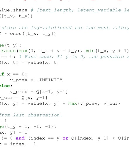
def monotonic_alignment_search(value):
”””Returns␣the␣most␣likely␣alignment␣for␣the␣given␣log-likelihood␣matrix.
␣␣␣␣Args:
␣␣␣␣␣␣␣␣value:␣the␣log-likelihood␣matrix.␣Its␣(i,␣j)-th␣entry␣contains
␣␣␣␣␣␣␣␣the␣log-likelihood␣of␣the␣j-th␣latent␣variable
␣␣␣␣␣␣␣␣for␣the␣given␣i-th␣prior␣mean␣and␣variance:
␣␣␣␣␣␣␣␣..␣math::
␣␣␣␣␣␣␣␣␣␣␣␣value_{i,j}␣=␣log␣N(f(z){j};␣\mu{i},␣\sigma_{i})
␣␣␣␣␣␣␣␣(dtype=float,␣shape=[text_length,␣latent_variable_length])
␣␣␣␣Returns:
␣␣␣␣␣␣␣␣path:␣the␣most␣likely␣alignment.
␣␣␣␣␣␣␣␣(dtype=float,␣shape=[text_length,␣latent_variable_length])
␣␣␣␣”””
t_x, t_y = value.shape # [text_length, letent_variable_length]
path = zeros([t_x, t_y])

# A cache to store the log-likelihood for the most likely alignment so far.
Q = -INFINITY * ones([t_x, t_y])

for y in range(t_y):
for x in range(max(0, t_x + y - t_y), min(t_x, y + 1)):
if y == 0: # Base case. If y is 0, the possible x value is only 0.
Q[x, 0] = value[x, 0]
else:
if x == 0:
v_prev = -INFINITY
else:
v_prev = Q[x-1, y-1]
v_cur = Q[x, y-1]
Q[x, y] = value[x, y] + max(v_prev, v_cur)

# Backtrack from last observation.
index = t_x - 1
for y in range(t_y - 1, -1, -1):
path[index, y] = 1
if index != 0 and (index == y or Q[index, y-1] < Q[index-1, y-1]):
index = index - 1

return path

Figure 4: Pseudocode for Monotonic Alignment Search.

def monotonic_alignment_search(value):
”””Returns␣the␣most␣likely␣alignment␣for␣the␣given␣log-likelihood␣matrix.
␣␣␣␣Args:
␣␣␣␣␣␣␣␣value:␣the␣log-likelihood␣matrix.␣Its␣(i,␣j)-th␣entry␣contains
␣␣␣␣␣␣␣␣the␣log-likelihood␣of␣the␣j-th␣latent␣variable
␣␣␣␣␣␣␣␣for␣the␣given␣i-th␣prior␣mean␣and␣variance:
␣␣␣␣␣␣␣␣..␣math::
␣␣␣␣␣␣␣␣␣␣␣␣value_{i,j}␣=␣log␣N(f(z){j};␣\mu{i},␣\sigma_{i})
␣␣␣␣␣␣␣␣(dtype=float,␣shape=[text_length,␣latent_variable_length])
␣␣␣␣Returns:
␣␣␣␣␣␣␣␣path:␣the␣most␣likely␣alignment.
␣␣␣␣␣␣␣␣(dtype=float,␣shape=[text_length,␣latent_variable_length])
␣␣␣␣”””
t_x, t_y = value.shape # [text_length, letent_variable_length]
path = zeros([t_x, t_y])

# A cache to store the log-likelihood for the most likely alignment so far.
Q = -INFINITY * ones([t_x, t_y])

for y in range(t_y):
for x in range(max(0, t_x + y - t_y), min(t_x, y + 1)):
if y == 0: # Base case. If y is 0, the possible x value is only 0.
Q[x, 0] = value[x, 0]
else:
if x == 0:
v_prev = -INFINITY
else:
v_prev = Q[x-1, y-1]
v_cur = Q[x, y-1]
Q[x, y] = value[x, y] + max(v_prev, v_cur)

# Backtrack from last observation.
index = t_x - 1
for y in range(t_y - 1, -1, -1):
path[index, y] = 1
if index != 0 and (index == y or Q[index, y-1] < Q[index-1, y-1]):
index = index - 1

return path

图 4：单调对齐搜索伪代码。

B. Model Configurations

B. 模型配置

In this section, we mainly describe the newly added parts of VITS as we followed configurations of Glow-TTS and HiFi-GAN for several parts of our model: we use the same transformer encoder and WaveNet residual blocks as those of Glow-TTS; our decoder and the multi-period discriminator is the same as the generator and multi-period discriminator of HiFi-GAN, respectively, except that we use different input dimension for the decoder and append a sub-discriminator.

本节主要描述 VITS 新加入的部分；模型若干部分沿用 Glow-TTS 与 HiFi-GAN 的配置：文本编码器与 WaveNet 残差块与 Glow-TTS 相同；解码器与多周期判别器分别与 HiFi-GAN 的生成器与多周期判别器相同，但解码器输入维不同，并追加了一个子判别器。

B.1. Prior Encoder and Posterior Encoder

B.1. 先验编码器与后验编码器

The normalizing flow in the prior encoder is a stack of four affine coupling layers, each coupling layer consisting of four WaveNet residual blocks. As we restrict the affine coupling layers to be volume-preserving transformations, the coupling layers do not produce scale parameters.

先验编码器中的归一化流是四层仿射耦合层的堆叠，每层耦合由四个 WaveNet 残差块组成。由于我们将仿射耦合层限制为保体积变换，耦合层不产出尺度参数。

The posterior encoder, consisting of 16 WaveNet residual blocks, takes linear-scale log magnitude spectrograms and produce latent variables with 192 channels.

后验编码器由 16 个 WaveNet 残差块组成，输入线性尺度对数幅度频谱，产出 192 通道的潜变量。

B.2. Decoder and Discriminator

B.2. 解码器与判别器

The input of our decoder is latent variables generated from the prior or posterior encoders, so the input channel size of the decoder is 192. For the last convolutional layer of the decoder, we remove a bias parameter, as it causes unstable gradient scales during mixed precision training.

解码器输入是先验或后验编码器生成的潜变量，因此输入通道数为 192。解码器最后一层卷积去掉偏置参数，因其在混合精度训练中会导致不稳定的梯度尺度。

For the discriminator, HiFi-GAN uses the multi-period discriminator containing five sub-discriminators with periods $[2,3,5,7,11]$ and the multi-scale discriminator containing three sub-discriminators. To improve training efficiency, we leave only the first sub-discriminator of the multi-scale discriminator that operates on raw waveforms and discard two sub-discriminators operating on average-pooled waveforms. The resultant discriminator can be seen as the multi-period discriminator with periods $[1,2,3,5,7,11]$.

判别器方面，HiFi-GAN 使用含周期 $[2,3,5,7,11]$ 的五个子判别器的多周期判别器，以及含三个子判别器的多尺度判别器。为提高训练效率，我们只保留多尺度判别器中作用于原始波形的第一个子判别器，丢弃两个作用于平均池化波形的子判别器。所得判别器可视为周期为 $[1,2,3,5,7,11]$ 的多周期判别器。

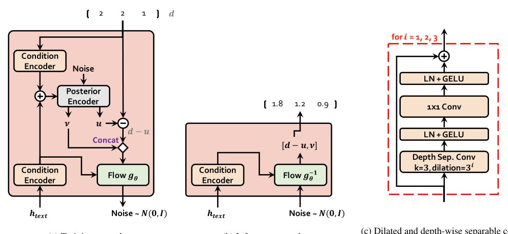
(a) Training procedure

（a）训练过程

B.3. Stochastic Duration Predictor

B.3. 随机时长预测器

Figures 5(a) and 5(b) show the training and inference procedures of the stochastic duration predictor, respectively. The main building block of the stochastic duration predictor is the dilated and depth-wise separable convolutional (DDSConv) residual block as in Figure 5(c). Each convolutional layer in DDSConv blocks is followed by a layer normalization layer and GELU activation function. We choose to use dilated and depth-wise separable convolutional layers for improving parameter efficiency while maintaining large receptive field size.

图 5(a) 与 5(b) 分别给出随机时长预测器的训练与推理过程。其主要构建块是如图 5(c) 所示的膨胀深度可分卷积（DDSConv）残差块。DDSConv 块中每个卷积层后接层归一化与 GELU 激活。我们选用膨胀与深度可分卷积，以便在保持大感受野的同时提高参数效率。

The posterior encoder and normalizing flow module in the duration predictor are flow-based neural networks and have the similar architecture. The difference is that the posterior encoder transforms a Gaussian noise sequence into two random variables $\nu$ and $u$ to express the approximate posterior distribution $q_{\phi}(u,\nu|d,c_{text})$, and the normalizing flow module transforms $d-u$ and $\nu$ into a Gaussian noise sequence to express the log-likelihood of the augmented and dequantized data $\log{p_{\theta}(d-u,\nu|c_{text})}$ as described in Section 2.2.2.

时长预测器中的后验编码器与归一化流模块都是基于流的神经网络，结构相近。差别在于：后验编码器把高斯噪声序列变换为两个随机变量 $\nu$ 与 $u$，以表达近似后验 $q_{\phi}(u,\nu|d,c_{text})$；归一化流模块则把 $d-u$ 与 $\nu$ 变换为高斯噪声序列，以表达增广并去量化后数据的对数似然 $\log{p_{\theta}(d-u,\nu|c_{text})}$，见第 2.2.2 节。

All input conditions are processed through condition encoders, each consisting of two 1x1 convolutional layers and a DDSConv residual block. The posterior encoder and normalizing flow module have four coupling layers of neural spline flows. Each coupling layer first processes input and input conditions through a DDSConv block and produces 29-channel parameters that are used to construct 10 rational-quadratic functions. We set the hidden dimension of all coupling layers and condition encoders to 192. Figure 6(a) and 6(b) show the architecture of a condition encoder and a coupling layer used in the stochastic duration predictor.

所有输入条件经条件编码器处理，每个条件编码器由两个 1×1 卷积层与一个 DDSConv 残差块组成。后验编码器与归一化流模块各有四层神经样条流耦合层。每层耦合先经 DDSConv 块处理输入与输入条件，再产出用于构造 10 个有理二次函数的 29 通道参数。所有耦合层与条件编码器的隐维设为 192。图 6(a) 与 6(b) 给出随机时长预测器中条件编码器与耦合层的结构。

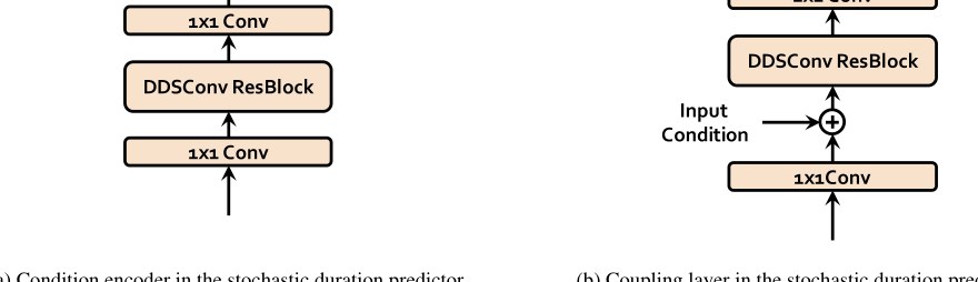
(a) Condition encoder in the stochastic duration predictor

（a）随机时长预测器中的条件编码器

C. Side-by-Side Evaluation

C. 并排评测

We conducted 7-point Comparative Mean Opinion Score (CMOS) evaluation between VITS and the ground truth through 500 ratings on 50 items. Our model achieved -0.106 and -0.270 CMOS on the LJ Speech and the VCTK datasets, respectively, as in Table 5. It indicates that even though our model outperforms the best publicly available TTS system, Glow-TTS and HiFi-GAN, and achieves a comparable score to ground truth in MOS evaluation, there remains a small preference of raters towards the ground truth over our model.

我们对 VITS 与真值做了 7 分比较平均意见分（CMOS）评测，共 50 个条目、500 次评分。如表 5，本模型在 LJ Speech 与 VCTK 上分别达到 -0.106 与 -0.270 CMOS。这表明即便本模型超过最佳公开 TTS 系统 Glow-TTS 与 HiFi-GAN，并在 MOS 评测中达到与真值可比的分数，评分者仍对真值相对本模型有轻微偏好。

Dataset	CMOS
LJ Speech	-0.106
VCTK	-0.262

Table 5: Evaluated CMOS of VITS compared to the ground truth.

数据集	CMOS
LJ Speech	-0.106
VCTK	-0.262

表 5：相对真值评测的 VITS CMOS。

D. Voice Conversion

D. 声音转换

In the multi-speaker setting, we do not provide speaker identities into the text encoder, which makes the latent variables estimated from the text encoder learn speaker-independent representations. Using the speaker-independent representations, we can transform an audio recording of one speaker into a voice of another speaker. For a given speaker identity $s$ and an utterance of the speaker, we can attain a linear spectrogram $x_{lin}$ from the corresponding utterance audio. We can transform $x_{lin}$ into a speaker-independent representation $e$ through the posterior encoder and the normalizing flow in the prior encoder:

在多说话人设定下，我们不向文本编码器提供说话人身份，使文本编码器估计的潜变量学到与说话人无关的表示。利用该表示，可将一位说话人的录音转换为另一位说话人的声音。给定说话人身份 $s$ 及其一条话语，可由对应音频得到线性频谱 $x_{lin}$。再经后验编码器与先验编码器中的归一化流，把 $x_{lin}$ 变换为与说话人无关的表示 $e$：

$$\displaystyle z \\ \displaystyle\sim q_{\phi}(z|x_{lin},s) \\ \displaystyle e \\ \displaystyle=f_{\theta}(z|s) \tag{12}$$

Then, we can synthesize a voice $\hat{y}$ of a target speaker identity $\hat{s}$ from the representation $e$ through the inverse transformation of the normalizing flow $f^{-1}_{\theta}$ and decoder $G$:

随后，经归一化流的逆变换 $f^{-1}_{\theta}$ 与解码器 $G$，可由表示 $e$ 合成目标说话人身份 $\hat{s}$ 的声音 $\hat{y}$：

$$\displaystyle\hat{y}=G(f_{\theta}^{-1}(e|\hat{s})|\hat{s}) \tag{14}$$

Learning speaker-independent representations and using it for voice conversion can be seen as an extension of the voice conversion method proposed in Glow-TTS. Our voice conversion method provides raw waveforms rather than mel-spectrograms as in Glow-TTS. The voice conversion results are presented in Figure 7. It shows a similar trend of pitch tracks with different pitch levels.

学习与说话人无关的表示并将其用于声音转换，可视为 Glow-TTS 所提声音转换方法的扩展。我们的声音转换直接给出原始波形，而非 Glow-TTS 中的梅尔频谱。声音转换结果见图 7：音高轨迹趋势相近，但音高水平不同。

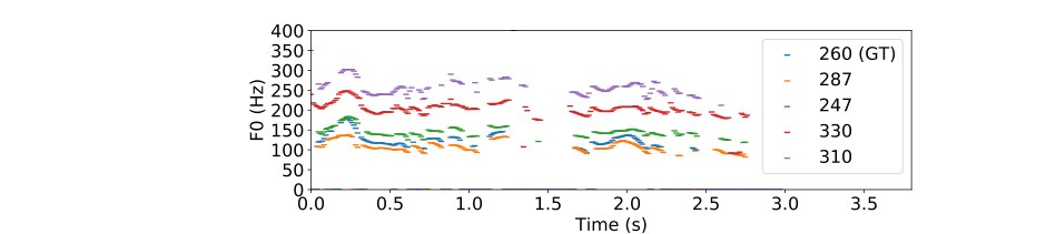
Figure 7: Pitch tracks of a ground truth sample and the corresponding voice conversion samples with different speaker identities.

图 7：真值样本与对应不同说话人身份声音转换样本的音高轨迹。