Visual Genome: Connecting Language and Vision Using Crowdsourced Dense Image Annotations
Int J Comput Vis (2017) 123:32–73
DOI 10.1007/s11263-016-0981-7
Visual Genome: Connecting Language and Vision Using Crowdsourced Dense Image Annotations
Visual Genome:用众包稠密图像标注连接语言与视觉
Received: 23 February 2016 / Accepted: 12 September 2016 / Published online: 6 February 2017
收稿日期:2016 年 2 月 23 日 / 接收日期:2016 年 9 月 12 日 / 在线发表:2017 年 2 月 6 日
© The Author(s) 2017. This article is published with open access at Springerlink.com
© 作者 2017。本文按开放获取方式发表于 Springerlink.com
Communicated by Margaret Mitchell, John Platt, and Kate Saenko.
B Ranjay Krishna
ranjaykrishna@cs.stanford.edu
¹ Stanford University, Stanford, CA, USA
² Dresden University of Technology, Dresden, Germany
³ Yahoo Inc., San Francisco, CA, USA
⁴ Snapchat Inc., Los Angeles, CA, USA
⁵ Centrum Wiskunde & Informatica (CWI), Amsterdam, The Netherlands
Abstract
摘要
Despite progress in perceptual tasks such as image classification, computers still perform poorly on cognitive tasks such as image description and question answering. Cognition is core to tasks that involve not just recognizing, but reasoning about our visual world. However, models used to tackle the rich content in images for cognitive tasks are still being trained using the same datasets designed for perceptual tasks. To achieve success at cognitive tasks, models need to understand the interactions and relationships between objects in an image. When asked “What vehicle is the person riding?”, computers will need to identify the objects in an image as well as the relationships riding(man, carriage) and pulling(horse, carriage) to answer correctly that “the person is riding a horse-drawn carriage.” In this paper, we present the Visual Genome dataset to enable the modeling of such relationships. We collect dense annotations of objects, attributes, and relationships within each image to learn these models. Specifically, our dataset contains over 108K images where each image has an average of objects, attributes, and pairwise relationships between objects. We canonicalize the objects, attributes, relationships, and noun phrases in region descriptions and questions answer pairs to WordNet synsets. Together, these annotations represent the densest and largest dataset of image descriptions, objects, attributes, relationships, and question answer pairs.
尽管图像分类等感知任务已有进展,计算机在图像描述和问答等认知任务上的表现仍然较差。认知是这类任务的核心:它们不只是识别,还要对我们的视觉世界进行推理。然而,用来处理图像中丰富内容、以完成认知任务的模型,仍在用当初为感知任务设计的数据集来训练。要在认知任务上取得成功,模型需要理解一幅图中物体之间的交互和关系。当被问到“What vehicle is the person riding?”时,计算机不但要识别图中的物体,还要抓住 riding(man, carriage) 和 pulling(horse, carriage) 这些关系,才能正确答出“the person is riding a horse-drawn carriage.”本文提出 Visual Genome 数据集,以便对这类关系建模。我们在每张图内收集物体、属性和关系的稠密标注,用来学习这些模型。具体而言,我们的数据集包含超过 10.8 万张图像,平均每张图有 个物体、 个属性和 对物体间的成对关系。我们把物体、属性、关系,以及区域描述和问答对中的名词短语,都规范化到 WordNet 同义词集。合在一起,这些标注构成了当时最密、也最大的图像描述、物体、属性、关系和问答对数据集。
Keywords Computer vision · Dataset · Image · Scene graph · Question answering · Objects · Attributes · Relationships · Knowledge · Language · Crowdsourcing
关键词 计算机视觉 · 数据集 · 图像 · 场景图 · 问答 · 物体 · 属性 · 关系 · 知识 · 语言 · 众包
1 Introduction
1 引言
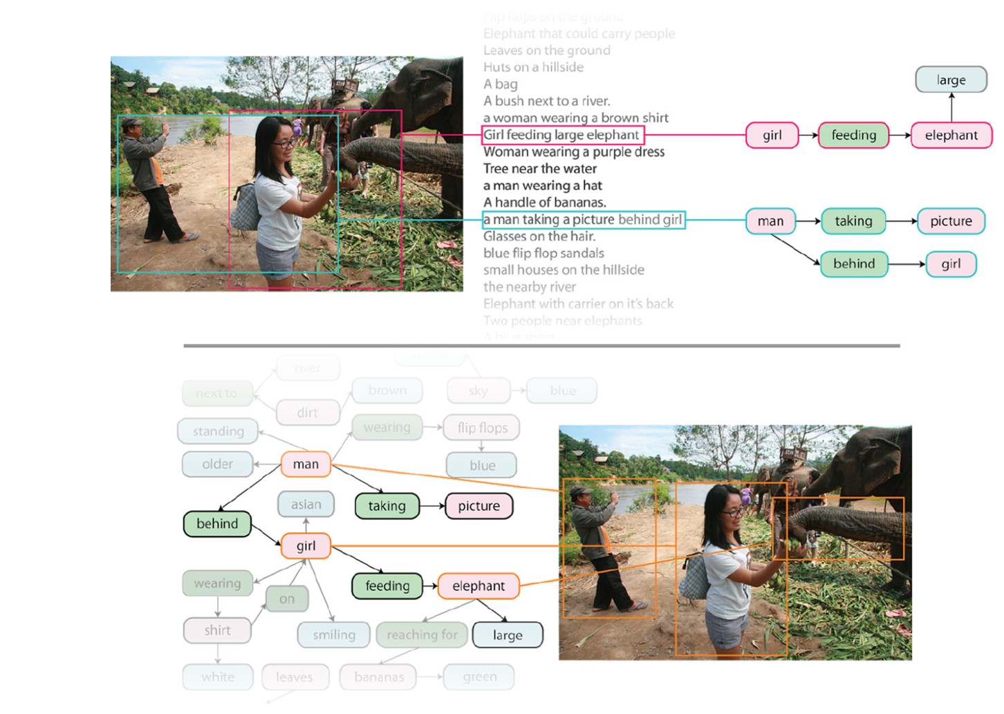
Fig. 1 An overview of the data needed to move from perceptual awareness to cognitive understanding of images. We present a dataset of images densely annotated with numerous region descriptions, objects, attributes, and relationships. Some examples of region descriptions (e.g. “girl feeding large elephant” and “a man taking a picture behind girl”) are shown (top). The objects (e.g. elephant), attributes (e.g. large) and relationships (e.g. feeding) are shown (bottom). Our dataset also contains image related question answer pairs (not shown)
图 1 从对图像的感知性觉察走向认知性理解所需数据的概览。我们给出一个带有大量区域描述、物体、属性和关系的稠密标注图像数据集。图中展示了一些区域描述的例子(如“girl feeding large elephant”和“a man taking a picture behind girl”)(上)。物体(如 elephant)、属性(如 large)和关系(如 feeding)显示在(下)。我们的数据集还包含与图像相关的问答对(未画出)。
A holy grail of computer vision is the complete understanding of visual scenes: a model that is able to name and detect objects, describe their attributes, and recognize their relationships. Understanding scenes would enable important applications such as image search, question answering, and robotic interactions. Much progress has been made in recent years towards this goal, including image classification (Perronnin et al. 2010; Simonyan and Zisserman 2014; Krizhevsky et al. 2012; Szegedy et al. 2015) and object detection (Girshick et al. 2014; Sermanet et al. 2013; Girshick 2015; Ren et al. 2015b). An important contributing factor is the availability of a large amount of data that drives the statistical models that underpin today’s advances in computational visual understanding. While the progress is exciting, we are still far from reaching the goal of comprehensive scene understanding. As Fig. 1 shows, existing models would be able to detect discrete objects in a photo but would not be able to explain their interactions or the relationships between them. Such explanations tend to be cognitive in nature, integrating perceptual information into conclusions about the relationships between objects in a scene (Bruner 1990; Firestone and Scholl 2015). A cognitive understanding of our visual world thus requires that we complement computers’ ability to detect objects with abilities to describe those objects (Isola et al. 2015) and understand their interactions within a scene (Sadeghi and Farhadi 2011).
计算机视觉的一个终极目标,是对视觉场景的完整理解:一个能够给物体命名并检测它们、描述其属性、并识别其关系的模型。理解场景将支撑图像检索、问答和机器人交互等重要应用。近年来朝着这一目标已有不少进展,包括图像分类(Perronnin et al. 2010; Simonyan and Zisserman 2014; Krizhevsky et al. 2012; Szegedy et al. 2015)和物体检测(Girshick et al. 2014; Sermanet et al. 2013; Girshick 2015; Ren et al. 2015b)。一个重要的推动因素,是大量数据的出现,它们驱动着支撑当前计算视觉理解进展的统计模型。进展令人振奋,但我们距离全面的场景理解仍很远。如图 1 所示,现有模型能够检测照片中一个个分立的物体,却无法解释它们的交互或彼此之间的关系。这类解释往往带有认知性质,要把感知信息整合进关于场景中物体关系的结论里(Bruner 1990; Firestone and Scholl 2015)。因此,要对我们的视觉世界形成认知性理解,就需要在计算机检测物体的能力之外,再补上描述这些物体(Isola et al. 2015)并理解它们在场景中交互(Sadeghi and Farhadi 2011)的能力。
There is an increasing effort to put together the next generation of datasets to serve as training and benchmarking datasets for these deeper, cognitive scene understanding and reasoning tasks, the most notable being MS-COCO (Lin et al. 2014) and VQA (Antol et al. 2015). The MS-COCO dataset consists of 300K real-world photos collected from Flickr. For each image, there is pixel-level segmentation of 80 object classes (when present) and 5 independent, user-generated sentences describing the scene. VQA adds to this a set of 614K question answer pairs related to the visual contents of each image (see more details in Sect. 3.1). With this information, MS-COCO and VQA provide a fertile training and testing ground for models aimed at tasks for accurate object detection, segmentation, and summary-level image captioning (Kiros et al. 2014; Mao et al. 2014; Karpathy and Fei-Fei 2015) as well as basic QA (Ren et al. 2015a; Malinowski et al. 2015; Gao et al. 2015; Malinowski and Fritz 2014). For example, a state-of-the-art model (Karpathy and Fei-Fei 2015) provides a description of one MS-COCO image in Fig. 1 as “two men are standing next to an elephant.” But what is missing is the further understanding of where each object is, what each person is doing, what the relationship between the person and elephant is, etc. Without such relationships, these models fail to differentiate this image from other images of people next to elephants.
为了给这些更深的、面向认知的场景理解和推理任务提供训练与基准数据集,把下一代数据集组织起来的努力正在增加,其中最突出的是 MS-COCO(Lin et al. 2014)和 VQA(Antol et al. 2015)。MS-COCO 数据集包含从 Flickr 收集的 30 万张真实世界照片。对每张图,有 80 个物体类别(在出现时)的像素级分割,以及 5 句由用户独立写出的场景描述。VQA 又为每张图的视觉内容增加了 61.4 万条问答对(详见第 3.1 节)。有了这些信息,MS-COCO 和 VQA 为旨在完成精确物体检测、分割和概要级图像配文(Kiros et al. 2014; Mao et al. 2014; Karpathy and Fei-Fei 2015)以及基本问答(Ren et al. 2015a; Malinowski et al. 2015; Gao et al. 2015; Malinowski and Fritz 2014)的模型,提供了肥沃的训练和测试土壤。例如,一个当时最好的模型(Karpathy and Fei-Fei 2015)把图 1 中的一张 MS-COCO 图像描述为“two men are standing next to an elephant.”但缺失的是对每个物体在哪里、每个人在做什么、人与象之间是什么关系等更进一步的理解。没有这些关系,这些模型就无法把这张图与其他“人在大象旁边”的图像区分开来。
To understand images thoroughly, we believe three key elements need to be added to existing datasets: a grounding of visual concepts to language (Kiros et al. 2014), a more complete set of descriptions and QAs for each image based on multiple image regions (Johnson et al. 2015), and a formalized representation of the components of an image (Hayes 1978). In the spirit of mapping out this complete information of the visual world, we introduce the Visual Genome dataset. The first release of the Visual Genome dataset uses images from the intersection of the YFCC100M (Thomee et al. 2016) and MS-COCO (Lin et al. 2014). Section 5 provides a more detailed description of the dataset. We highlight below the motivation and contributions of the three key elements that set Visual Genome apart from existing datasets.
要透彻理解图像,我们认为现有数据集还需要补上三个关键要素:把视觉概念接地到语言(Kiros et al. 2014),基于多个图像区域、为每张图提供更完整的一组描述和问答(Johnson et al. 2015),以及对图像组成部分的一种形式化表示(Hayes 1978)。本着把视觉世界的这类完整信息描绘出来的精神,我们推出 Visual Genome 数据集。Visual Genome 的首个发布版本使用了 YFCC100M(Thomee et al. 2016)与 MS-COCO(Lin et al. 2014)交集中的 张图像。第 5 节对数据集有更详细的说明。下面我们强调把 Visual Genome 与现有数据集区分开来的三个关键要素的动机和贡献。
The Visual Genome dataset regards relationships and attributes as first-class citizens of the annotation space, in addition to the traditional focus on objects. Recognition of relationships and attributes is an important part of the complete understanding of the visual scene, and in many cases, these elements are key to the story of a scene (e.g., the difference between “a dog chasing a man” versus “a man chasing a dog”). The Visual Genome dataset is among the first to provide a detailed labeling of object interactions and attributes, grounding visual concepts to language.¹
除了传统上对物体的关注之外,Visual Genome 数据集把关系和属性视为标注空间中的一等公民。识别关系和属性是完整理解视觉场景的重要部分,而且在许多情况下,这些要素是场景故事的关键(例如,“a dog chasing a man”与“a man chasing a dog”之间的差别)。Visual Genome 是较早提供物体交互与属性详细标注、从而把视觉概念接地到语言的数据集之一。¹
¹ The Lotus Hill Dataset (Yao et al. 2007) also provides a similar annotation of object relationships, see Sec. 3.1.
¹ Lotus Hill 数据集(Yao et al. 2007)也提供了类似的物体关系标注,见第 3.1 节。
An image is often a rich scenery that cannot be fully described in one summarizing sentence. The scene in Fig. 1 contains multiple “stories”: “a man taking a photo of elephants,” “a woman feeding an elephant,” “a river in the background of lush grounds,” etc. Existing datasets such as Flickr 30K (Young et al. 2014) and MS-COCO (Lin et al. 2014) focus on high-level descriptions of an image.² Instead, for each image in the Visual Genome dataset, we collect more than descriptions for different regions in the image, providing a much denser and more complete set of descriptions of the scene. In addition, inspired by VQA (Antol et al. 2015), we also collect an average of 17 question answer pairs based on the descriptions for each image. Region-based question answers can be used to jointly develop NLP and vision models that can answer questions from either the description or the image, or both of them.
一幅图像往往是丰富的景致,无法用一句总括性的话完全说清。图 1 中的场景包含多个“故事”:“a man taking a photo of elephants”、“a woman feeding an elephant”、“a river in the background of lush grounds”等。Flickr 30K(Young et al. 2014)和 MS-COCO(Lin et al. 2014)等现有数据集关注的是图像的高层描述。² 与此不同,Visual Genome 中的每张图,我们都为图中不同区域收集了超过 条描述,从而提供更密、也更完整的一组场景描述。此外,受 VQA(Antol et al. 2015)启发,我们还基于每张图的描述平均收集 17 条问答对。基于区域的问答可以用来共同发展自然语言处理和视觉模型,使它们能够从描述或图像、或从两者同时出发来回答问题。
² COCO has multiple sentences generated independently by different users, all focusing on providing an overall, one sentence description of the scene.
² COCO 中有多句由不同用户独立写成的句子,都着眼于给场景提供一句总体描述。
With a set of dense descriptions of an image and the explicit correspondences between visual pixels (i.e. bounding boxes of objects) and textual descriptors (i.e. relationships, attributes), the Visual Genome dataset is poised to be the first image dataset that is capable of providing a structured formalized representation of an image, in the form that is widely used in knowledge base representations in NLP (Zhou et al. 2007; GuoDong et al. 2005; Culotta and Sorensen 2004; Socher et al. 2012). For example, in Fig. 1, we can formally express the relationship holding between the woman and food as holding(woman, food). Putting together all the objects and relations in a scene, we can represent each image as a scene graph (Johnson et al. 2015). The scene graph representation has been shown to improve semantic image retrieval (Johnson et al. 2015; Schuster et al. 2015) and image captioning (Farhadi et al. 2009; Chang et al. 2014; Gupta and Davis 2008). Furthermore, all objects, attributes and relationships in each image in the Visual Genome dataset are canonicalized to its corresponding WordNet (Miller 1995) ID (called a synset ID). This mapping connects all images in Visual Genome and provides an effective way to consistently query the same concept (object, attribute, or relationship) in the dataset. It can also potentially help train models that can learn from contextual information from multiple images (Figs. 2, 3).
有了一组稠密的图像描述,以及视觉像素(即物体边界框)与文本描述符(即关系、属性)之间的显式对应,Visual Genome 有条件成为第一个能够提供结构化形式化图像表示的图像数据集,其形式与自然语言处理中知识库表示所广泛使用的形式一致(Zhou et al. 2007; GuoDong et al. 2005; Culotta and Sorensen 2004; Socher et al. 2012)。例如,在图 1 中,我们可以把 woman 与 food 之间的关系 holding 形式化地表示为 holding(woman, food)。把场景中的全部物体和关系放在一起,我们就可以把每张图表示成一张场景图(Johnson et al. 2015)。场景图表示已被证明可以改进语义图像检索(Johnson et al. 2015; Schuster et al. 2015)和图像配文(Farhadi et al. 2009; Chang et al. 2014; Gupta and Davis 2008)。此外,Visual Genome 中每张图的所有物体、属性和关系都被规范化到对应的 WordNet(Miller 1995)编号(称为同义词集 ID)。这种映射把 Visual Genome 中的所有图像连接起来,并提供了一种在数据集中一致查询同一概念(物体、属性或关系)的有效方法。它也有可能帮助训练能够从多张图像的上下文信息中学习的模型(图 2、图 3)。
In this paper, we introduce the Visual Genome dataset with the aim of training and benchmarking the next generation of computer models for comprehensive scene understanding. The paper proceeds as follows: In Sect. 2, we provide a detailed description of each component of the dataset. Section 3 provides a literature review of related datasets as well as related recognition tasks. Section 4 discusses the crowdsourcing strategies we deployed in the ongoing effort of collecting this dataset. Section 5 is a collection of data analysis statistics, showcasing the key properties of the Visual Genome dataset. Last but not least, Sect. 6 provides a set of experimental results that use Visual Genome as a benchmark.
本文介绍 Visual Genome 数据集,目的是为全面场景理解的下一代计算机模型提供训练和基准。论文安排如下:第 2 节详细说明数据集的各个组成部分。第 3 节综述相关数据集以及相关识别任务。第 4 节讨论我们在持续收集该数据集过程中部署的众包策略。第 5 节汇集数据分析统计,展示 Visual Genome 数据集的关键性质。最后,第 6 节给出一组把 Visual Genome 当作基准的实验结果。
Further visualizations, API, and additional information on the Visual Genome dataset can be found online.³
关于 Visual Genome 数据集的更多可视化、API 和其他信息,可在网上找到。³
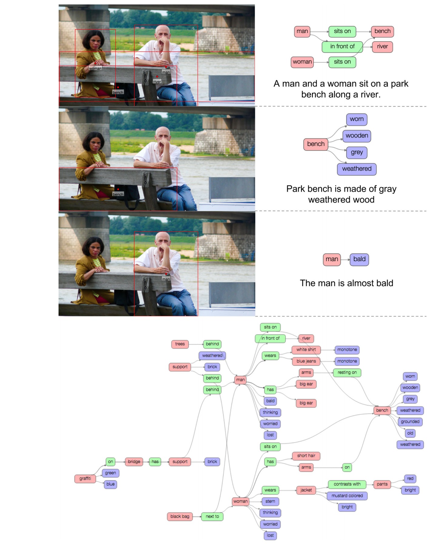
Fig. 2 An example image from the Visual Genome dataset. We show 3 region descriptions and their corresponding region graphs. We also show the connected scene graph collected by combining all of the image’s region graphs. The top region description is “a man and a woman sit on a park bench along a river.” It contains the objects: man, woman, bench and river. The relationships that connect these objects are: sits_on(man, bench), in_front_of(man, river), and sits_on(woman, bench)
图 2 Visual Genome 数据集中的一张示例图像。我们展示了 3 条区域描述及其对应的区域图,并展示了把该图全部区域图合并后得到的连通场景图。上方区域的描述是“a man and a woman sit on a park bench along a river.”其中包含物体:man、woman、bench 和 river。连接这些物体的关系是:sits_on(man, bench)、in_front_of(man, river),以及 sits_on(woman, bench)。
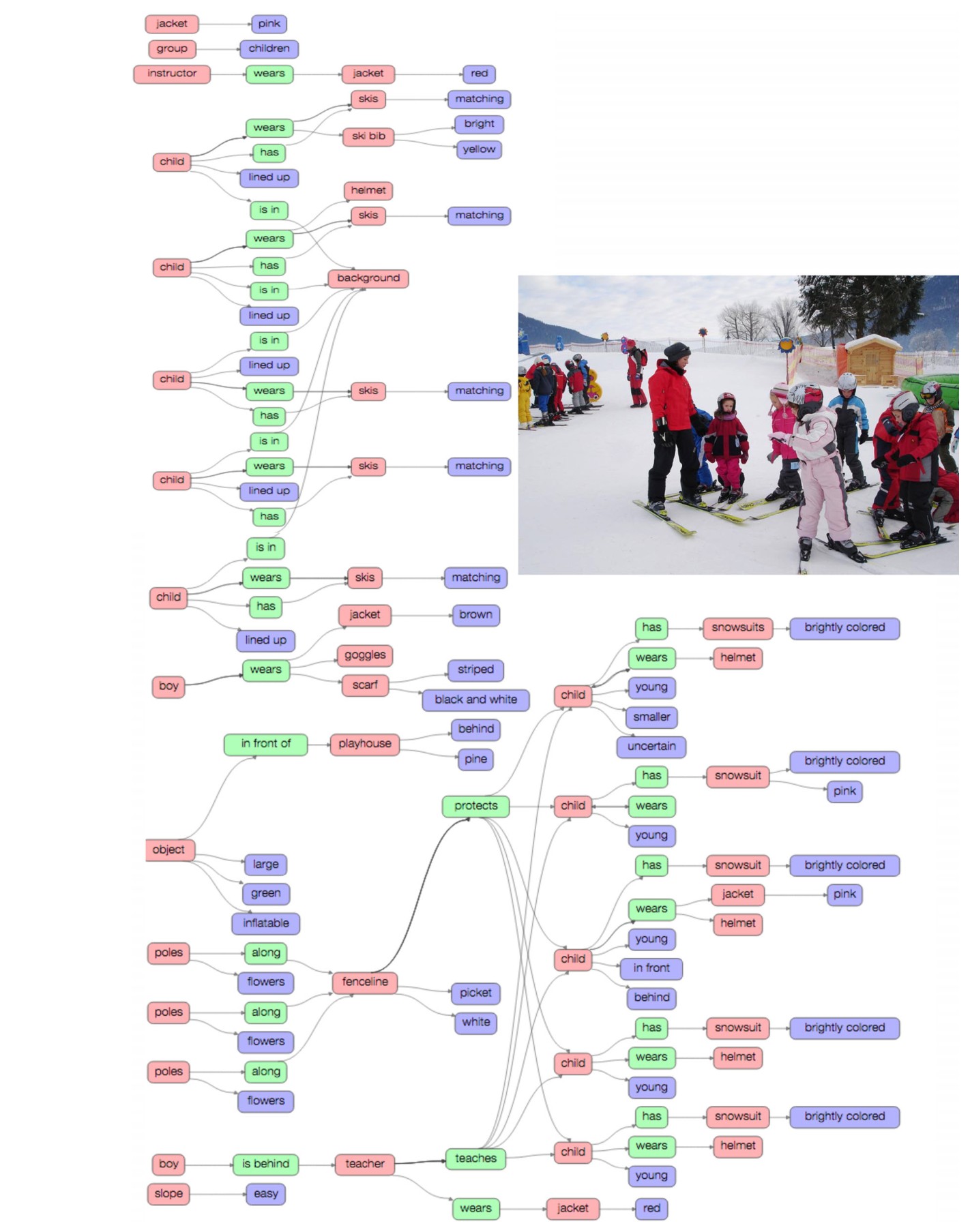
Fig. 3 An example image from our dataset along with its scene graph representation. The scene graph contains objects (child, instructor, helmet, etc.) that are localized in the image as bounding boxes (not shown). These objects also have attributes: large, green, behind, etc. Finally, objects are connected to each other through relationships: wears(child, helmet), wears(instructor, jacket), etc
图 3 我们数据集中的一张示例图像及其场景图表示。场景图包含物体(child、instructor、helmet 等),它们在图像中以边界框定位(未画出)。这些物体还带有属性:large、green、behind 等。最后,物体通过关系彼此相连:wears(child, helmet)、wears(instructor, jacket) 等。
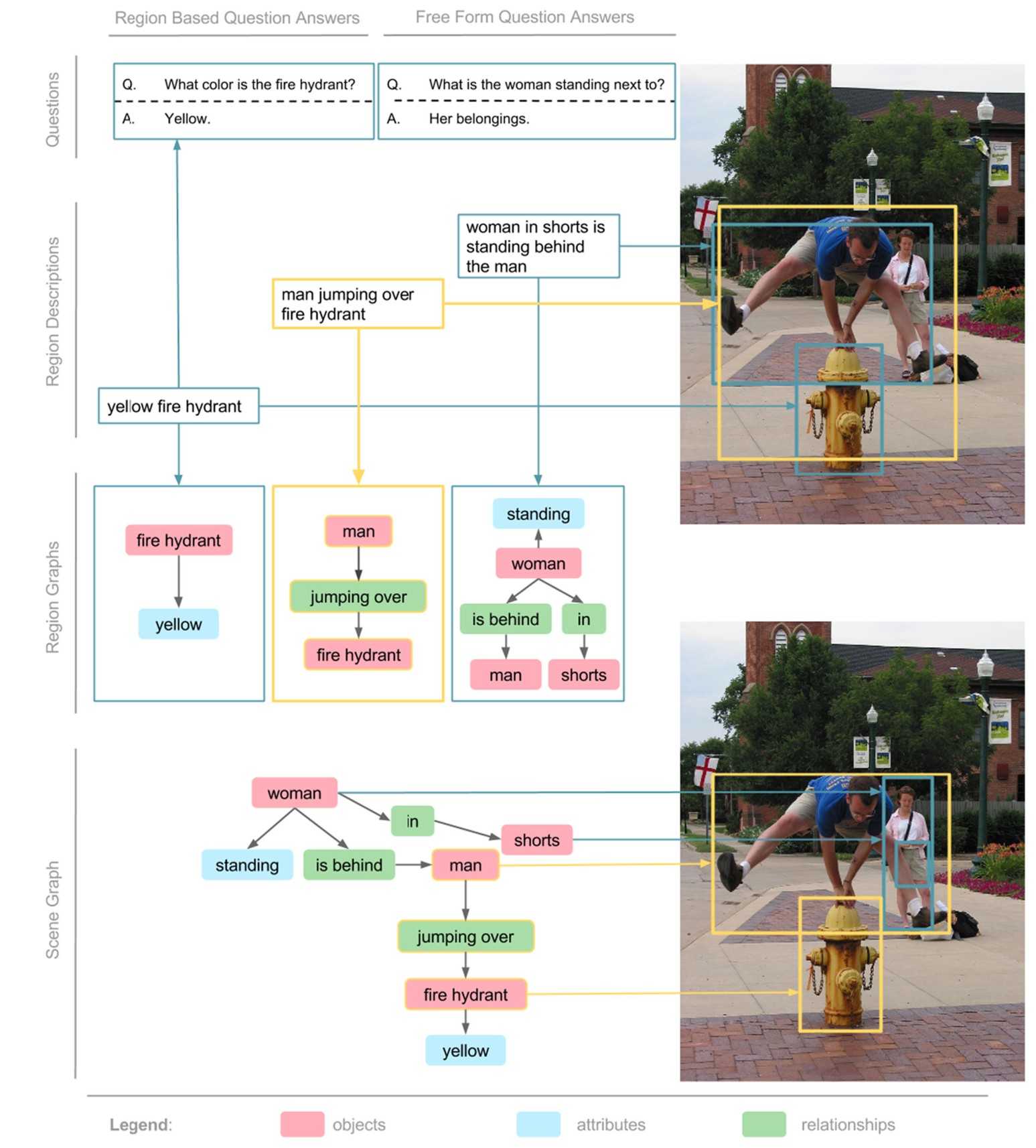
Fig. 4 A representation of the Visual Genome dataset. Each image contains region descriptions that describe a localized portion of the image. We collect two types of question answer pairs (QAs): freeform QAs and region-based QAs. Each region is converted to a region graph representation of objects, attributes, and pairwise relationships. Finally, each of these region graphs are combined to form a scene graph with all the objects grounded to the image. Best viewed in color
图 4 Visual Genome 数据集的一种表示。每张图像都包含描述局部区域的区域描述。我们收集两类问答对(QA):自由形式问答和基于区域的问答。每个区域被转换成由物体、属性和成对关系组成的区域图。最后,这些区域图合并成一张场景图,其中所有物体都接地到图像上。建议查看彩色图。
2 Visual Genome Data Representation
2 Visual Genome 的数据表示
The Visual Genome dataset consists of seven main components: region descriptions, objects, attributes, relationships, region graphs, scene graphs, and question answer pairs. Figure 4 shows examples of each component for one image. To enable research on comprehensive understanding of images, we begin by collecting descriptions and question answers. These are raw texts without any restrictions on length or vocabulary. Next, we extract objects, attributes and relationships from our descriptions. Together, objects, attributes and relationships comprise our scene graphs that represent a formal representation of an image. In this section, we break down Fig. 4 and explain each of the seven components. In Sect. 4, we will describe in more detail how data from each component is collected through a crowdsourcing platform.
Visual Genome 数据集由七个主要部分组成:区域描述、物体、属性、关系、区域图、场景图和问答对。图 4 给出了一张图上各部分的例子。为了推动对图像的全面理解研究,我们先收集描述和问答。这些都是原始文本,对长度或词表没有限制。接下来,我们从描述中抽出物体、属性和关系。物体、属性和关系合在一起,构成作为图像形式化表示的场景图。在本节中,我们把图 4 拆开,逐一说明这七个部分。在第 4 节,我们将更详细地说明每个部分的数据是如何通过众包平台收集的。
2.1 Multiple Regions and Their Descriptions
2.1 多个区域及其描述
In a real-world image, one simple summary sentence is often insufficient to describe all the contents of and interactions in an image. Instead, one natural way to extend this might be a collection of descriptions based on different regions of a scene. In Visual Genome, we collect diverse human-generated image region descriptions, with each region localized by a bounding box. In Fig. 5, we show three examples of region descriptions. Regions are allowed to have a high degree of overlap with each other when the descriptions differ. For example, “yellow fire hydrant” and “woman in shorts is standing behind the man” have very little overlap, while “man jumping over fire hydrant” has a very high overlap with the other two regions. Our dataset contains on average a total of region descriptions per image. Each description is a phrase ranging from to words in length describing that region.
在真实世界的图像中,一句简单的总括往往不足以描述图中的全部内容和交互。一种自然的扩展,或许是基于场景不同区域的一组描述。在 Visual Genome 中,我们收集多样的、由人工写出的图像区域描述,每个区域都用边界框定位。在图 5 中,我们展示了三条区域描述的例子。当描述不同时,区域之间允许有很高的重叠。例如,“yellow fire hydrant”与“woman in shorts is standing behind the man”几乎没有重叠,而“man jumping over fire hydrant”与另外两个区域有很高的重叠。我们的数据集平均每张图共有 条区域描述。每条描述是一个长度为 到 个词的短语,用来描写该区域。
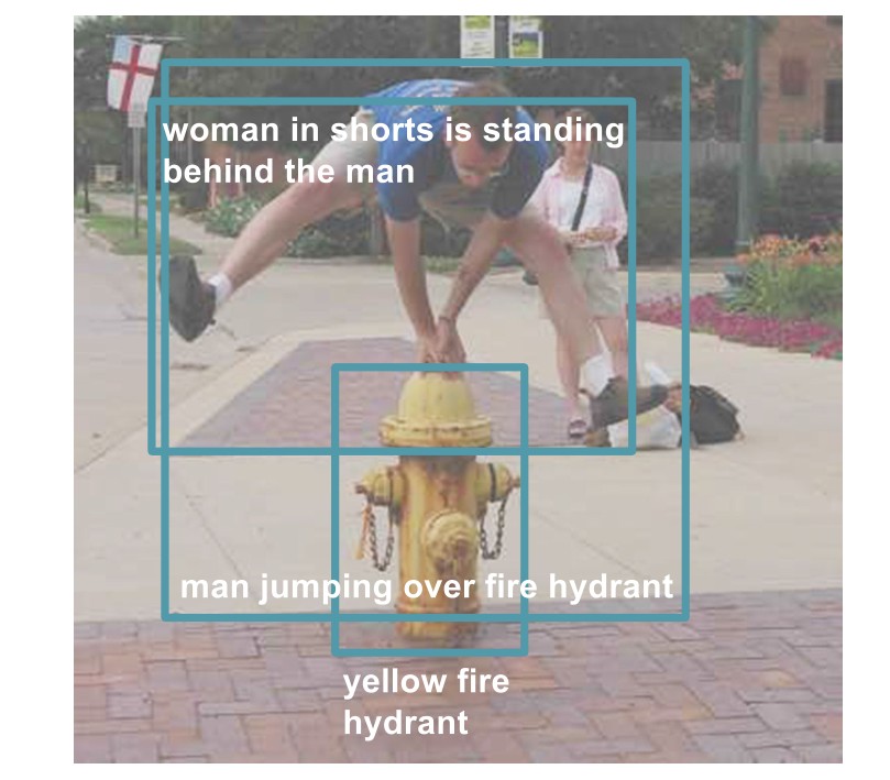
Fig. 5 To describe all the contents of and interactions in an image, the Visual Genome dataset includes multiple human-generated image regions descriptions, with each region localized by a bounding box. Here, we show three regions descriptions on various image regions: “man jumping over a fire hydrant,” “yellow fire hydrant,” and “woman in shorts is standing behind the man”
图 5 为了描述一幅图中的全部内容和交互,Visual Genome 数据集包含多条由人工写出的图像区域描述,每个区域都用边界框定位。这里我们展示了三条落在不同区域上的描述:“man jumping over a fire hydrant”、“yellow fire hydrant”,以及“woman in shorts is standing behind the man”。
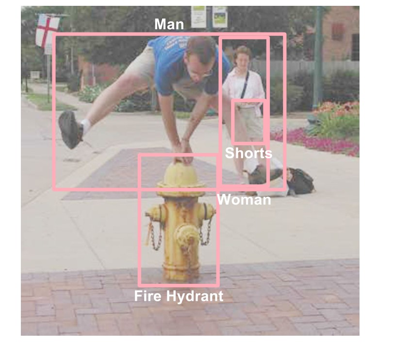
Fig. 6 From all of the region descriptions, we extract all objects mentioned. For example, from the region description “man jumping over a fire hydrant,” we extract man and fire hydrant
图 6 我们从全部区域描述中抽出提到的所有物体。例如,从区域描述“man jumping over a fire hydrant”中,我们抽出 man 和 fire hydrant。
2.2 Multiple Objects and Their Bounding Boxes
2.2 多个物体及其边界框
Each image in our dataset consists of an average of objects, each delineated by a tight bounding box (Fig. 6). Furthermore, each object is canonicalized to a synset ID in WordNet (Miller 1995). For example, man would get mapped to man.n.03 (the generic use of the word to refer to any human being). Similarly, person gets mapped to person.n.01 (a human being). Afterwards, these two concepts can be joined to person.n.01 since this is a hypernym of man.n.03. We did not standardize synsets in our dataset. However, given our canonicalization, this is easily possible leveraging the WordNet ontology to avoid multiple names for one object (e.g. man, person, human), and to connect information across images.
我们数据集中的每张图平均包含 个物体,每个物体都用紧致边界框圈出(图 6)。此外,每个物体都被规范化到 WordNet(Miller 1995)中的一个同义词集 ID。例如,man 会被映射到 man.n.03 (the generic use of the word to refer to any human being)。类似地,person 被映射到 person.n.01 (a human being)。之后,这两个概念可以归并到 person.n.01,因为这是 man.n.03 的上位词。我们没有在数据集中把同义词集标准化。不过,有了我们的规范化,利用 WordNet 本体可以很容易做到这一点,从而避免同一个物体有多个名称(如 man、person、human),并把跨图像的信息连接起来。
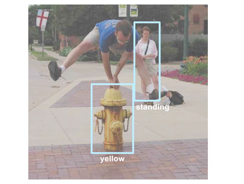
Fig. 7 Some descriptions also provide attributes for objects. For example, the region description “yellow fire hydrant” adds that the fire hydrant is yellow. Here we show two attributes: yellow and standing
图 7 有些描述还为物体提供属性。例如,区域描述“yellow fire hydrant”补充说明这个 fire hydrant 是 yellow。这里我们展示了两个属性:yellow 和 standing。
2.3 A Set of Attributes
2.3 一组属性
Each image in Visual Genome has an average of attributes. Objects can have zero or more attributes associated with them. Attributes can be color (e.g. yellow), states (e.g. standing), etc. (Fig. 7). Just like we collect objects from region descriptions, we also collect the attributes attached to these objects. In Fig. 7, from the phrase “yellow fire hydrant,” we extract the attribute yellow for the fire hydrant. As with objects, we canonicalize all attributes to WordNet (Miller 1995); for example, yellow is mapped to yellow.s.01 (of the color intermediate between green and orange in the color spectrum; of something resembling the color of an egg yolk).
Visual Genome 中的每张图平均有 个属性。物体可以关联零个或多个属性。属性可以是颜色(如 yellow)、状态(如 standing)等(图 7)。正如我们从区域描述中收集物体一样,我们也收集附着在这些物体上的属性。在图 7 中,我们从短语“yellow fire hydrant”中为 fire hydrant 抽出属性 yellow。与物体一样,我们把所有属性都规范化到 WordNet(Miller 1995);例如,yellow 被映射到 yellow.s.01 (of the color intermediate between green and orange in the color spectrum; of something resembling the color of an egg yolk)。
2.4 A Set of Relationships
2.4 一组关系
Relationships connect two objects together. These relationships can be actions (e.g. jumping over), spatial (e.g. is behind), descriptive verbs (e.g. wear), prepositions (e.g. with), comparative (e.g. taller than), or prepositional phrases (e.g. drive on). For example, from the region description “man jumping over fire hydrant,” we extract the relationship jumping over between the objects man and fire hydrant (Fig. 8). These relationships are directed from one object, called the subject, to another, called the object. In this case, the subject is the man, who is performing the relationship jumping over on the object fire hydrant. Each relationship is canonicalized to a WordNet (Miller 1995) synset ID; i.e. jumping is canonicalized to jump.a.1 (move forward by leaps and bounds). On average, each image in our dataset contains relationships.
关系把两个物体连接在一起。这些关系可以是动作(如 jumping over)、空间关系(如 is behind)、描述性动词(如 wear)、介词(如 with)、比较(如 taller than),或介词短语(如 drive on)。例如,从区域描述“man jumping over fire hydrant”中,我们抽出物体 man 与 fire hydrant 之间的关系 jumping over(图 8)。这些关系从一个称为主语的物体指向另一个称为宾语的物体。在这个例子中,主语是 man,它在宾语 fire hydrant 上执行关系 jumping over。每个关系都被规范化到一个 WordNet(Miller 1995)同义词集 ID;也就是说,jumping 被规范化到 jump.a.1 (move forward by leaps and bounds)。平均而言,我们数据集中的每张图包含 个关系。
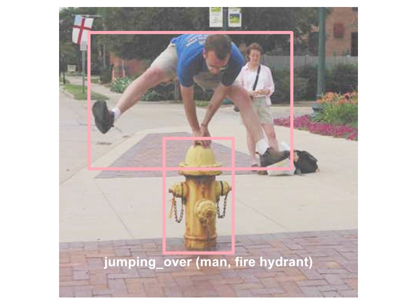
Fig. 8 Our dataset also captures the relationships and interactions between objects in our images. In this example, we show the relationship jumping over between the objects man and fire hydrant
图 8 我们的数据集还刻画了图像中物体之间的关系和交互。在这个例子中,我们展示了物体 man 与 fire hydrant 之间的关系 jumping over。
2.5 A Set of Region Graphs
2.5 一组区域图
Combining the objects, attributes, and relationships extracted from region descriptions, we create a directed graph representation for each of the regions. Examples of region graphs are shown in Fig. 4. Each region graph is a structured representation of a part of the image. The nodes in the graph represent objects, attributes, and relationships. Objects are linked to their respective attributes while relationships link one object to another. The links connecting two objects in Fig. 4 point from the subject to the relationship and from the relationship to the other object.
把从区域描述中抽出的物体、属性和关系组合起来,我们为每个区域建立一个有向图表示。区域图的例子见图 4。每张区域图都是图像一部分的结构化表示。图中的节点表示物体、属性和关系。物体连接到各自的属性,而关系把一个物体连向另一个物体。图 4 中连接两个物体的边,从主语指向关系,再从关系指向另一个物体。
2.6 One Scene Graph
2.6 一张场景图
While region graphs are localized representations of an image, we also combine them into a single scene graph representing the entire image (Fig. 3). The scene graph is the union of all region graphs and contains all objects, attributes, and relationships from each region description. By doing so, we are able to combine multiple levels of scene information in a more coherent way. For example in Fig. 4, the leftmost region description tells us that the “fire hydrant is yellow,” while the middle region description tells us that the “man is jumping over the fire hydrant.” Together, the two descriptions tell us that the “man is jumping over a yellow fire hydrant.”
区域图是图像的局部化表示,我们还把它们合并成一张表示整幅图像的场景图(图 3)。场景图是所有区域图的并集,包含每条区域描述中的全部物体、属性和关系。这样一来,我们就能把多层场景信息以更连贯的方式组合起来。例如在图 4 中,最左边的区域描述告诉我们“fire hydrant is yellow”,中间的区域描述告诉我们“man is jumping over the fire hydrant”。合在一起,两条描述告诉我们“man is jumping over a yellow fire hydrant”。
2.7 A Set of Question Answer Pairs
2.7 一组问答对
We have two types of QA pairs associated with each image in our dataset: freeform QAs, based on the entire image, and region-based QAs, based on selected regions of the image. We collect 6 different types of questions per image: what, where, how, when, who, and why. In Fig. 4, “Q. What is the woman standing next to?; A. Her belongings” is a freeform QA. Each image has at least one question of each type listed above. Region-based QAs are collected by prompting workers with region descriptions. For example, we use the region “yellow fire hydrant” to collect the region-based QA: “Q. What color is the fire hydrant?; A. Yellow.” Region based QAs are based on the description and allow us to independently study how well models perform at answering questions using the image or the region description as input.
我们的数据集中,每张图都关联两类问答对:基于整张图的自由形式问答,以及基于所选区域的区域问答。我们为每张图收集 6 种不同类型的问题:what、where、how、when、who 和 why。在图 4 中,“Q. What is the woman standing next to?; A. Her belongings”是一条自由形式问答。每张图对上面列出的每种类型至少有一个问题。区域问答是通过向工人出示区域描述来收集的。例如,我们用区域“yellow fire hydrant”收集到区域问答:“Q. What color is the fire hydrant?; A. Yellow.”区域问答以描述为基础,使我们能够分别研究模型在以图像或以区域描述作为输入时回答问题的表现。
3 Related Work
3 相关工作
We discuss existing datasets that have been released and used by the vision community for classification and object detection. We also mention work that has improved object and attribute detection models. Then, we explore existing work that has utilized representations similar to our relationships between objects. In addition, we dive into literature related to cognitive tasks like image description, question answering, and knowledge representation.
我们讨论视觉社区已经发布并用于分类和物体检测的现有数据集,也提到改进了物体和属性检测模型的工作。然后,我们考察利用了与我们的物体间关系相类似的表示的已有工作。此外,我们还会进入与图像描述、问答和知识表示等认知任务相关的文献。
Table 1 A comparison of existing datasets with Visual Genome
| Dataset | Images | Descriptions per image | Total objects | # Object categories | Objects per image | # Attributes categories | Attributes per image | # Relationship categories | Relationships per image | Question answers |
|---|---|---|---|---|---|---|---|---|---|---|
| YFCC100M (Thomee et al. 2016) | 100,000,000 | – | – | – | – | – | – | – | – | – |
| Tiny images (Torralba et al. 2008) | 80,000,000 | – | – | 53,464 | 1 | – | – | – | – | – |
| ImageNet (Deng et al. 2009) | 14,197,122 | – | 14,197,122 | 21,841 | 1 | – | – | – | – | – |
| ILSVRC detection (2012) (Russakovsky et al. 2015) | 476,688 | – | 534,309 | 200 | 2.5 | – | – | – | – | – |
| MS-COCO (Lin et al. 2014) | 328,000 | 5 | 27,472 | 80 | – | – | – | – | – | – |
| Flickr 30K (Young et al. 2014) | 31,783 | 5 | – | – | – | – | – | – | – | – |
| Caltech 101 (Fei-Fei et al. 2007) | 9144 | – | 9144 | 102 | 1 | – | – | – | – | – |
| Caltech 256 (Griffin et al. 2007) | 30,608 | – | 30,608 | 257 | 1 | – | – | – | – | – |
| Caltech pedestrian (Dollar et al. 2012) | 250,000 | – | 350,000 | 1 | 1.4 | – | – | – | – | – |
| Pascal detection (Everingham et al. 2010) | 11,530 | – | 27,450 | 20 | 2.38 | – | – | – | – | – |
| Abstract scenes (Zitnick and Parikh 2013) | 10,020 | – | 58 | 11 | 5 | – | – | – | – | – |
| aPascal (Farhadi et al. 2009) | 12,000 | – | – | – | – | 64 | – | – | – | – |
| Animal attributes (Lampert et al. 2009) | 30,000 | – | – | – | – | 1,280 | – | – | – | – |
| SUN attributes (Patterson et al. 2014) | 14,000 | – | – | – | – | 700 | 700 | – | – | – |
| Caltech birds (Wah et al. 2011) | 11,788 | – | – | – | – | 312 | 312 | – | – | – |
| COCO actions (Ronchi and Perona 2015) | 10,000 | – | – | – | 5.2 | – | – | 156 | 20.7 | – |
| Visual phrases (Sadeghi and Farhadi 2011) | – | – | – | – | – | – | – | 17 | 1 | – |
| VisKE (Sadeghi et al. 2015) | – | – | – | – | – | – | – | 6500 | – | – |
| DAQUAR (Malinowski and Fritz 2014) | 1,449 | – | – | – | – | – | – | – | – | 12,468 |
| COCO QA (Ren et al. 2015a) | 123,287 | – | – | – | – | – | – | – | – | 117,684 |
| Baidu (Gao et al. 2015) | 120,360 | – | – | – | – | – | – | – | – | 250,569 |
| VQA (Antol et al. 2015) | 204,721 | – | – | – | – | – | – | – | – | 614,163 |
| Visual Genome | 108,077 | 50 | 3,843,636 | 33,877 | 35 | 68,111 | 26 | 42,374 | 21 | 1,773,258 |
We show that Visual Genome has an order of magnitude more descriptions and question answers. It also has a more diverse set of object, attribute, and relationship classes. Additionally, Visual Genome contains a higher density of these annotations per image. The number of distinct categories in Visual Genome are calculated by lower-casing and stemming names of objects, attributes and relationships.
表 1 现有数据集与 Visual Genome 的比较
| 数据集 | 图像数 | 每图描述数 | 物体总数 | 物体类别数 | 每图像物体数 | 属性类别数 | 每图像属性数 | 关系类别数 | 每图像关系数 | 问答数 |
|---|---|---|---|---|---|---|---|---|---|---|
| YFCC100M (Thomee et al. 2016) | 100,000,000 | – | – | – | – | – | – | – | – | – |
| Tiny images (Torralba et al. 2008) | 80,000,000 | – | – | 53,464 | 1 | – | – | – | – | – |
| ImageNet (Deng et al. 2009) | 14,197,122 | – | 14,197,122 | 21,841 | 1 | – | – | – | – | – |
| ILSVRC detection (2012) (Russakovsky et al. 2015) | 476,688 | – | 534,309 | 200 | 2.5 | – | – | – | – | – |
| MS-COCO (Lin et al. 2014) | 328,000 | 5 | 27,472 | 80 | – | – | – | – | – | – |
| Flickr 30K (Young et al. 2014) | 31,783 | 5 | – | – | – | – | – | – | – | – |
| Caltech 101 (Fei-Fei et al. 2007) | 9144 | – | 9144 | 102 | 1 | – | – | – | – | – |
| Caltech 256 (Griffin et al. 2007) | 30,608 | – | 30,608 | 257 | 1 | – | – | – | – | – |
| Caltech pedestrian (Dollar et al. 2012) | 250,000 | – | 350,000 | 1 | 1.4 | – | – | – | – | – |
| Pascal detection (Everingham et al. 2010) | 11,530 | – | 27,450 | 20 | 2.38 | – | – | – | – | – |
| Abstract scenes (Zitnick and Parikh 2013) | 10,020 | – | 58 | 11 | 5 | – | – | – | – | – |
| aPascal (Farhadi et al. 2009) | 12,000 | – | – | – | – | 64 | – | – | – | – |
| Animal attributes (Lampert et al. 2009) | 30,000 | – | – | – | – | 1,280 | – | – | – | – |
| SUN attributes (Patterson et al. 2014) | 14,000 | – | – | – | – | 700 | 700 | – | – | – |
| Caltech birds (Wah et al. 2011) | 11,788 | – | – | – | – | 312 | 312 | – | – | – |
| COCO actions (Ronchi and Perona 2015) | 10,000 | – | – | – | 5.2 | – | – | 156 | 20.7 | – |
| Visual phrases (Sadeghi and Farhadi 2011) | – | – | – | – | – | – | – | 17 | 1 | – |
| VisKE (Sadeghi et al. 2015) | – | – | – | – | – | – | – | 6500 | – | – |
| DAQUAR (Malinowski and Fritz 2014) | 1,449 | – | – | – | – | – | – | – | – | 12,468 |
| COCO QA (Ren et al. 2015a) | 123,287 | – | – | – | – | – | – | – | – | 117,684 |
| Baidu (Gao et al. 2015) | 120,360 | – | – | – | – | – | – | – | – | 250,569 |
| VQA (Antol et al. 2015) | 204,721 | – | – | – | – | – | – | – | – | 614,163 |
| Visual Genome | 108,077 | 50 | 3,843,636 | 33,877 | 35 | 68,111 | 26 | 42,374 | 21 | 1,773,258 |
我们表明,Visual Genome 的描述和问答数量高出一个数量级。它的物体、属性和关系类别也更丰富。此外,Visual Genome 中这些标注在每张图上的密度也更高。Visual Genome 中的不同类别数,是通过对物体、属性和关系名称做小写化和词干提取后计算得到的。
3.1 Datasets
3.1 数据集
Datasets (Table 1) have been growing in size as researchers have begun tackling increasingly complicated problems. Caltech 101 (Fei-Fei et al. 2007) was one of the first datasets hand-curated for image classification, with 101 object categories and 15–30 examples per category. One of the biggest criticisms of Caltech 101 was the lack of variability in its examples. Caltech 256 (Griffin et al. 2007) increased the number of categories to 256, while also addressing some of the shortcomings of Caltech 101. However, it still had only a handful of examples per category, and most of its images contained only a single object. LabelMe (Russell et al. 2008) introduced a dataset with multiple objects per category. They also provided a web interface that experts and novices could use to annotate additional images. This web interface enabled images to be labeled with polygons, helping create datasets for image segmentation. The Lotus Hill dataset (Yao et al. 2007) contains a hierarchical decomposition of objects (vehicles, man-made objects, animals, etc.) along with segmentations. Only a small part of this dataset is freely available. SUN (Xiao et al. 2010), just like LabelMe (Russell et al. 2008) and Lotus Hill (Yao et al. 2007), was curated for object detection. Pushing the size of datasets even further, 80 Million Tiny Images (Torralba et al. 2008) created a significantly larger dataset than its predecessors. It contains tiny (i.e. pixels) images that were collected using WordNet (Miller 1995) synsets as queries. However, because the data in 80 Million Images were not human-verified, they contain numerous errors. YFCC100M (Thomee et al. 2016) is another large database of 100 million images that is still largely unexplored. It contains human generated and machine generated tags.
随着研究者开始处理日益复杂的问题,数据集(表 1)的规模也在增大。Caltech 101(Fei-Fei et al. 2007)是最早为图像分类手工整理的数据集之一,有 101 个物体类别,每类 15–30 个例子。对 Caltech 101 最大的批评之一,是其例子缺少变化。Caltech 256(Griffin et al. 2007)把类别数增加到 256,同时也应对了 Caltech 101 的一些不足。不过,它每个类别仍然只有少量例子,而且大多数图像只包含单个物体。LabelMe(Russell et al. 2008)推出了一个每类有多个物体的数据集。他们还提供了一个专家和新手都可以用来为更多图像标注的网页界面。这个网页界面可以用多边形给图像贴标签,从而帮助创建图像分割数据集。Lotus Hill 数据集(Yao et al. 2007)包含物体(车辆、人造物体、动物等)的层次分解以及分割。该数据集只有一小部分可免费获取。SUN(Xiao et al. 2010)和 LabelMe(Russell et al. 2008)、Lotus Hill(Yao et al. 2007)一样,是为物体检测整理的。把数据集规模再往前推,80 Million Tiny Images(Torralba et al. 2008)创建了比前人显著更大的数据集。它包含用 WordNet(Miller 1995)同义词集作为查询收集来的微小图像(即 像素)。不过,因为 80 Million Images 中的数据未经人工核验,其中有大量错误。YFCC100M(Thomee et al. 2016)是另一个包含 1 亿张图像的大型数据库,目前在很大程度上仍未得到充分探索。它包含人工生成和机器生成的标签。
Pascal VOC (Everingham et al. 2010) pushed research from classification to object detection with a dataset containing 20 semantic categories in 11, 000 images. ImageNet (Deng et al. 2009) took WordNet synsets and crowdsourced a large dataset of 14 million images. They started the ILSVRC (Russakovsky et al. 2015) challenge for a variety of computer vision tasks. Together, ILSVRC and PASCAL provide a test bench for object detection, image classification, object segmentation, person layout, and action classification. MS-COCO (Lin et al. 2014) recently released its dataset, with over 328, 000 images with sentence descriptions and segmentations of 80 object categories. The previous largest dataset for image-based QA, VQA (Antol et al. 2015), contains 204,721 images annotated with three question answer pairs. They collected a dataset of 614,163 freeform questions with 6.1M ground truth answers (10 per question) and provided a baseline approach in answering questions using an image and a textual question as the input.
Pascal VOC(Everingham et al. 2010)用一个包含 11,000 张图像、20 个语义类别的数据集,把研究从分类推向物体检测。ImageNet(Deng et al. 2009)以 WordNet 同义词集为基础,众包了一个 1400 万张图像的大型数据集。他们发起了面向多种计算机视觉任务的 ILSVRC(Russakovsky et al. 2015)挑战赛。ILSVRC 和 PASCAL 一起,为物体检测、图像分类、物体分割、人物布局和动作分类提供了测试台。MS-COCO(Lin et al. 2014)最近发布了其数据集,包含超过 328,000 张带句子描述、并对 80 个物体类别做了分割的图像。此前最大的基于图像的问答数据集 VQA(Antol et al. 2015)包含 204,721 张图像,每张标注了三对问答。他们收集了 614,163 个自由形式问题及 610 万条真值答案(每个问题 10 条),并给出了一种以图像和文本问题为输入来回答问题的基线方法。
Visual Genome aims to bridge the gap between all these datasets, collecting not just annotations for a large number of objects but also scene graphs, region descriptions, and question answer pairs for image regions. Unlike previous datasets, which were collected for a single task like image classification, the Visual Genome dataset was collected to be a general-purpose representation of the visual world, without bias toward a particular task. Our images contain an average of objects, which is almost an order of magnitude more dense than any existing vision dataset. Similarly, we contain an average of attributes and relationships per image. We also have an order of magnitude more unique objects, attributes, and relationships than any other dataset. Finally, we have million question answer pairs, also larger than any other dataset for visual question answering.
Visual Genome 旨在弥合这些数据集之间的缺口,不仅为大量物体收集标注,还为图像区域收集场景图、区域描述和问答对。与以往为图像分类这类单一任务收集的数据集不同,Visual Genome 被收集成视觉世界的一种通用表示,并不偏向某一特定任务。我们的图像平均包含 个物体,密度几乎比任何现有视觉数据集高出一个数量级。类似地,平均每张图有 个属性和 个关系。在独特的物体、属性和关系数量上,我们也比其他任何数据集高出一个数量级。最后,我们有 万条问答对,规模也大于其他视觉问答数据集。
3.2 Image Descriptions
3.2 图像描述
One of the core contributions of Visual Genome is its descriptions for multiple regions in an image. As such, we mention other image description datasets and models in this subsection. Most work related to describing images can be divided into two categories: retrieval of human-generated captions and generation of novel captions. Methods in the first category use similarity metrics between image features from predefined models to retrieve similar sentences (Ordonez et al. 2011; Hodosh et al. 2013). Other methods map both sentences and their images to a common vector space (Ordonez et al. 2011) or map them to a space of triples (Farhadi et al. 2010). Among those in the second category, a common theme has been to use recurrent neural networks to produce novel captions (Kiros et al. 2014; Mao et al. 2014; Karpathy and Fei-Fei 2015; Vinyals et al. 2015; Chen and Lawrence Zitnick 2015; Donahue et al. 2015; Fang et al. 2015). More recently, researchers have also used a visual attention model (Xu et al. 2015).
Visual Genome 的核心贡献之一,是为一幅图中的多个区域提供描述。因此,我们在本小节提到其他图像描述数据集和模型。与描述图像相关的大多数工作可以分为两类:检索人工写出的配文,以及生成新的配文。第一类方法使用来自预定义模型的图像特征之间的相似性度量,来检索相近的句子(Ordonez et al. 2011; Hodosh et al. 2013)。另一些方法把句子及其图像映射到一个共同的向量空间(Ordonez et al. 2011),或映射到三元组空间(Farhadi et al. 2010)。在第二类方法中,一个常见主题是用循环神经网络生成新的配文(Kiros et al. 2014; Mao et al. 2014; Karpathy and Fei-Fei 2015; Vinyals et al. 2015; Chen and Lawrence Zitnick 2015; Donahue et al. 2015; Fang et al. 2015)。最近,研究者也使用了视觉注意力模型(Xu et al. 2015)。
One drawback of these approaches is their attention to describing only the most salient aspect of the image. This problem is amplified by datasets like Flickr 30K (Young et al. 2014) and MS-COCO (Lin et al. 2014), whose sentence desriptions tend to focus, somewhat redundantly, on these salient parts. For example, “an elephant is seen wandering around on a sunny day,” “a large elephant in a tall grass field,” and “a very large elephant standing alone in some brush” are 3 descriptions from the MS-COCO dataset, and all of them focus on the salient elephant in the image and ignore the other regions in the image. Many real-world scenes are complex, with multiple objects and interactions that are best described using multiple descriptions (Karpathy and Fei-Fei 2015; Lebret et al. 2015). Our dataset pushes toward a more complete understanding of an image by collecting a dataset in which we capture not just scene-level descriptions but also myriad of low-level descriptions, the “grammar” of the scene.
这些方法的一个缺点,是它们往往只描述图像中最显著的方面。Flickr 30K(Young et al. 2014)和 MS-COCO(Lin et al. 2014)这类数据集进一步放大了这个问题,它们的句子描述往往有些重复地聚焦在这些显著部分上。例如,“an elephant is seen wandering around on a sunny day”、“a large elephant in a tall grass field”和“a very large elephant standing alone in some brush”是 MS-COCO 数据集中的 3 条描述,它们都聚焦在图中那头显著的大象上,而忽略了图中的其他区域。许多真实世界场景很复杂,有多个物体和交互,最适合用多条描述来刻画(Karpathy and Fei-Fei 2015; Lebret et al. 2015)。我们的数据集推动对图像更完整的理解:我们收集的数据不仅有场景级描述,还有大量低层描述,也就是场景的“语法”。
3.3 Objects
3.3 物体
Object detection is a fundamental task in computer vision, with applications ranging from identification of faces in photo software to identification of other cars by self-driving cars on the road. It involves classifying an object into a distinct category and localizing the object in the image. Visual Genome uses objects as a core component on which each visual scene is built. Early datasets include the face detection (Huang et al. 2008) and pedestrian datasets (Dollar et al. 2012). The PASCAL VOC and ILSVRC’s detection dataset pushed research in object detection. But the images in these datasets are iconic and do not capture the settings in which these objects usually co-occur. To remedy this problem, MS-COCO (Lin et al. 2014) annotated real-world scenes that capture object contexts. However, MS-COCO was unable to describe all the objects in its images, since they annotated only 80 object categories. In the real world, there are many more objects that the ones captured by existing datasets. Visual Genome aims at collecting annotations for all visual elements that occur in images, increasing the number of distinct categories to .
物体检测是计算机视觉中的一项基础任务,应用范围从照片软件中的人脸识别,到自动驾驶汽车在路上识别其他车辆。它包括把物体分到一个明确的类别,并在图像中定位该物体。Visual Genome 把物体作为构建每个视觉场景的核心组成部分。早期的数据集包括人脸检测(Huang et al. 2008)和行人数据集(Dollar et al. 2012)。PASCAL VOC 和 ILSVRC 的检测数据集推动了物体检测研究。但这些数据集中的图像偏于典型,没有捕捉这些物体通常共同出现的场景。为了弥补这一点,MS-COCO(Lin et al. 2014)标注了能够捕捉物体上下文的真实世界场景。不过,MS-COCO 无法描述其图像中的全部物体,因为他们只标注了 80 个物体类别。在真实世界中,物体远比现有数据集所覆盖的要多。Visual Genome 旨在为图像中出现的全部视觉元素收集标注,把不同类别数增加到 。
3.4 Attributes
3.4 属性
The inclusion of attributes allows us to describe, compare, and more easily categorize objects. Even if we haven’t seen an object before, attributes allow us to infer something about it; for example, “yellow and brown spotted with long neck” likely refers to a giraffe. Initial work in this area involved finding objects with similar features (Malisiewicz et al. 2008) using examplar SVMs. Next, textures were used to study objects (Varma and Zisserman 2005), while other methods learned to predict colors (Ferrari and Zisserman 2007). Finally, the study of attributes was explicitly demonstrated to lead to improvements in object classification (Farhadi et al. 2009). Attributes were defined to be parts (e.g. “has legs”), shapes (e.g. “spherical”), or materials (e.g. “furry”) and could be used to classify new categories of objects. Attributes have also played a large role in improving fine-grained recognition (Goering et al. 2014) on fine-grained attribute datasets like CUB-2011 (Wah et al. 2011). In Visual Genome, we use a generalized formulation (Johnson et al. 2015), but we extend it such that attributes are not image-specific binaries but rather object-specific for each object in a real-world scene. We also extend the types of attributes to include size (e.g. “small”), pose (e.g. “bent”), state (e.g. “transparent”), emotion (e.g. “happy”), and many more.
加入属性后,我们就可以描述、比较并更容易地给物体归类。即使以前没见过某个物体,属性也能让我们推断一些信息;例如,“yellow and brown spotted with long neck”很可能指的是长颈鹿。这一方向的早期工作包括用 exemplar SVM 寻找具有相似特征的物体(Malisiewicz et al. 2008)。接下来,纹理被用来研究物体(Varma and Zisserman 2005),另一些方法则学习预测颜色(Ferrari and Zisserman 2007)。最后,对属性的研究被明确证明可以改进物体分类(Farhadi et al. 2009)。属性被定义成部件(如“has legs”)、形状(如“spherical”)或材料(如“furry”),可以用来分类新的物体类别。属性在改进细粒度识别方面也发挥了很大作用(Goering et al. 2014),相关的细粒度属性数据集如 CUB-2011(Wah et al. 2011)。在 Visual Genome 中,我们使用一种一般化的表述(Johnson et al. 2015),但加以扩展,使属性不再是针对整张图的二值标记,而是针对真实世界场景中每个物体的、物体特定的标注。我们还扩展了属性类型,使其包括大小(如“small”)、姿态(如“bent”)、状态(如“transparent”)、情绪(如“happy”)等许多种类。
3.5 Relationships
3.5 关系
Relationship extraction has been a traditional problem in information extraction and in natural language processing. Syntactic features (Zhou et al. 2007; GuoDong et al. 2005), dependency tree methods (Culotta and Sorensen 2004; Bunescu and Mooney 2005), and deep neural networks (Socher et al. 2012; Zeng et al. 2014) have been employed to extract relationships between two entities in a sentence. However, in computer vision, very little work has gone into learning or predicting relationships. Instead, relationships have been implicitly used to improve other vision tasks. Relative layouts between objects have improved scene categorization (Izadinia et al. 2014), and 3D spatial geometry between objects has helped object detection (Choi et al. 213). Comparative adjectives and prepositions between pairs of objects have been used to model visual relationships and improved object localization (Gupta and Davis 2008).
关系抽取是信息抽取和自然语言处理中的传统问题。句法特征(Zhou et al. 2007; GuoDong et al. 2005)、依存树方法(Culotta and Sorensen 2004; Bunescu and Mooney 2005)以及深度神经网络(Socher et al. 2012; Zeng et al. 2014)都被用来抽取句子中两个实体之间的关系。然而在计算机视觉中,学习或预测关系的工作还很少。相反,关系往往被隐式地用来改进其他视觉任务。物体之间的相对布局改进了场景分类(Izadinia et al. 2014),物体之间的三维空间几何则帮助了物体检测(Choi et al. 213)。比较形容词和介词被用来对成对物体之间的视觉关系建模,并改进了物体定位(Gupta and Davis 2008)。
Relationships have already shown their utility in improving visual cognitive tasks (Antol et al. 2014; Yang et al. 2012). A meaning space of relationships has improved the mapping of images to sentences (Farhadi et al. 2010). Relationships in a structured representation with objects have been defined as a graph structure called a scene graph, where the nodes are objects with attributes and edges are relationships between objects. This representation can be used to generate indoor images from sentences and also to improve image search (Chang et al. 2014; Johnson et al. 2015). We use a similar scene graph representation of an image that generalizes across all these previous works (Johnson et al. 2015). Recently, relationships have come into focus again in the form of question answering about associations between objects (Sadeghi et al. 2015). These questions ask if a relationship, involving generally two objects, is true, e.g. “do dogs eat ice cream?”. We believe that relationships will be necessary for higher-level cognitive tasks (Johnson et al. 2015; Lu et al. 2016), so we collect the largest corpus of them in an attempt to improve tasks by actually understanding interactions between objects.
关系已经显示出它们在改进视觉认知任务方面的用处(Antol et al. 2014; Yang et al. 2012)。一个有意义的关系空间改进了从图像到句子的映射(Farhadi et al. 2010)。带有物体的结构化表示中的关系,被定义成一种称为场景图的图结构,其中节点是带属性的物体,边是物体之间的关系。这种表示可以用来从句子生成室内图像,也可以改进图像检索(Chang et al. 2014; Johnson et al. 2015)。我们使用一种类似的图像场景图表示,它概括了这些先前工作(Johnson et al. 2015)。最近,关系再次成为关注点,形式是关于物体之间关联的问答(Sadeghi et al. 2015)。这些问题通常问涉及两个物体的某种关系是否成立,例如“do dogs eat ice cream?”。我们相信,更高层的认知任务将需要关系(Johnson et al. 2015; Lu et al. 2016),因此我们收集了规模最大的这类语料,试图通过真正理解物体之间的交互来改进这些任务。
3.6 Question Answering
3.6 问答
Visual question answering (QA) has been recently proposed as a proxy task of evaluating a computer vision system’s ability to understand an image beyond object recognition and image captioning (Geman et al. 2015; Malinowski and Fritz 2014). Several visual QA benchmarks have been proposed in the last few months. The DAQUAR (Malinowski and Fritz 2014) dataset was the first toy-sized QA benchmark built upon indoor scene RGB-D images of NYU Depth v2 (Nathan Silberman and Fergus 2012). Most new datasets (Yu et al. 2015; Ren et al. 2015a; Antol et al. 2015; Gao et al. 2015) have collected QA pairs on MS-COCO images, either generated automatically by NLP tools (Ren et al. 2015a) or written by human workers (Yu et al. 2015; Antol et al. 2015; Gao et al. 2015).
视觉问答(QA)最近被提出来,作为评估计算机视觉系统在物体识别和图像配文之外理解图像能力的一项代理任务(Geman et al. 2015; Malinowski and Fritz 2014)。过去几个月里已经提出了若干视觉问答基准。DAQUAR(Malinowski and Fritz 2014)数据集是建立在 NYU Depth v2(Nathan Silberman and Fergus 2012)室内场景 RGB-D 图像上的第一个玩具规模问答基准。大多数新数据集(Yu et al. 2015; Ren et al. 2015a; Antol et al. 2015; Gao et al. 2015)都在 MS-COCO 图像上收集问答对,要么由自然语言处理工具自动生成(Ren et al. 2015a),要么由人工写出(Yu et al. 2015; Antol et al. 2015; Gao et al. 2015)。
In previous datasets, most questions concentrated on simple recognition-based questions about the salient objects, and answers were often extremely short. For instance, of DAQUAR answers (Malinowski and Fritz 2014) and of VQA answers (Antol et al. 2015) consist of single-word object names, attributes, and quantities. This limitation bounds their diversity and fails to capture the long-tail details of the images. Given the availability of new datasets, an array of visual QA models have been proposed to tackle QA tasks. The proposed models range from SVM classifiers and probabilistic inference (Malinowski and Fritz 2014) to recurrent neural networks (Gao et al. 2015; Malinowski et al. 2015; Ren et al. 2015a) and convolutional networks (Ma et al. 2015). Visual Genome aims to capture the details of the images with diverse question types and long answers. These questions should cover a wide range of visual tasks from basic perception to complex reasoning. Our QA dataset of million QAs is also larger than any currently existing dataset.
在以往的数据集中,大多数问题集中在关于显著物体的简单识别类问题上,答案往往极短。例如,DAQUAR 中 的答案(Malinowski and Fritz 2014)以及 VQA 中 的答案(Antol et al. 2015)都由单个词的物体名、属性和数量组成。这一限制束缚了它们的多样性,也未能捕捉图像中的长尾细节。随着新数据集的出现,已有一系列视觉问答模型被提出来应对问答任务。这些模型从 SVM 分类器和概率推断(Malinowski and Fritz 2014),到循环神经网络(Gao et al. 2015; Malinowski et al. 2015; Ren et al. 2015a)和卷积网络(Ma et al. 2015)。Visual Genome 旨在用多样的问题类型和较长的答案来捕捉图像细节。这些问题应当覆盖从基本感知到复杂推理的广泛视觉任务。我们包含 万条问答的问答数据集,规模也大于目前已有的任何数据集。
3.7 Knowledge Representation
3.7 知识表示
A knowledge representation of the visual world is capable of tackling an array of vision tasks, from action recognition to general question answering. However, it is difficult to answer “what is the minimal viable set of knowledge needed to understand about the physical world?” (Hayes 1978). It was later proposed that there be a certain plurality to concepts and their related axioms (Hayes 1985). These efforts have grown to model physical processes (Forbus 1984) or to model a series of actions as scripts (Schank and Abelson 2013) for stories—both of which are not depicted in a single static image but which play roles in an image’s story (Vedantam et al. 2015b). More recently, NELL (Betteridge et al. 2009) learns probabilistic horn clauses by extracting information from the web. DeepQA (Ferrucci et al. 2010) proposes a probabilistic question answering architecture involving over 100 different techniques. Others have used Markov logic networks (Zhu et al. 2009; Niu et al. 2012) as their representation to perform statistical inference for knowledge base construction. Our work is most similar to that of those (Chen et al. 2013; Zhu et al. 2014, 2015; Sadeghi et al. 2015) who attempt to learn common-sense relationships from images. Visual Genome scene graphs can also be considered a dense knowledge representation for images. It is similar to the format used in knowledge bases in NLP.
视觉世界的知识表示能够应对从动作识别到一般问答的一系列视觉任务。然而,很难回答“理解物理世界所需的最小可行知识集合是什么?”(Hayes 1978)。后来有人提出,概念及其相关公理应具有某种多元性(Hayes 1985)。这些努力已扩展到对物理过程建模(Forbus 1984),或把一系列动作建模成故事中的脚本(Schank and Abelson 2013)——这两者都不会出现在单张静态图像中,却在图像的故事里发挥作用(Vedantam et al. 2015b)。更近一些,NELL(Betteridge et al. 2009)通过从网页抽取信息来学习概率霍恩子句。DeepQA(Ferrucci et al. 2010)提出一种涉及 100 多种不同技术的概率问答架构。另一些工作则用马尔可夫逻辑网络(Zhu et al. 2009; Niu et al. 2012)作为表示,对知识库构建做统计推断。我们的工作与那些试图从图像中学习常识关系的研究最为相近(Chen et al. 2013; Zhu et al. 2014, 2015; Sadeghi et al. 2015)。Visual Genome 的场景图也可以看作图像的一种稠密知识表示,其格式与自然语言处理中知识库所用的格式相似。
4 Crowdsourcing Strategies
4 众包策略
Visual Genome was collected and verified entirely by crowd workers from Amazon Mechanical Turk. In this section, we outline the pipeline employed in creating all the components of the dataset. Each component (region descriptions, objects, attributes, relationships, region graphs, scene graphs, questions and answers) involved multiple task stages. We mention the different strategies used to make our data accurate and to enforce diversity in each component. We also provide background information about the workers who helped make Visual Genome possible.
Visual Genome 完全由 Amazon Mechanical Turk 上的众包工人收集并核验。本节概述创建数据集各个部分时所采用的流程。每个部分(区域描述、物体、属性、关系、区域图、场景图、问题与答案)都包含多个任务阶段。我们会说明为了保证数据准确、并在每个部分中强制多样性而使用的不同策略。我们也会介绍帮助 Visual Genome 成为可能的那些工人的背景信息。
4.1 Crowd Workers
4.1 众包工人
We used Amazon Mechanical Turk (AMT) as our primary source of annotations. Overall, a total of over 33, 000 unique workers contributed to the dataset. The dataset was collected over the course of 6 months after 15 months of experimentation and iteration on the data representation. Approximately 800, 000 Human Intelligence Tasks (HITs) were launched on AMT, where each HIT involved creating descriptions, questions and answers, or region graphs. Each HIT was designed such that workers manage to earn anywhere between 8 per hour if they work continuously, in line with ethical research standards on Mechanical Turk (Salehi et al. 2015). Visual Genome HITs achieved a 94.1% retention rate, meaning that 94.1% of workers who completed one of our tasks went ahead to do more. Table 2 outlines the percentage distribution of the locations of the workers. 93.02% of workers contributed from the United States.
我们以 Amazon Mechanical Turk(AMT)作为主要标注来源。总体而言,共有超过 33,000 名独特工人为该数据集做出了贡献。在对数据表示进行了 15 个月的试验和迭代之后,数据集的采集历时 6 个月。大约 80 万项人类智能任务(HIT)在 AMT 上发布,每项 HIT 涉及创建描述、问答,或区域图。每项 HIT 的设计使工人如果连续工作,时薪可以达到 6 到 8 美元,符合在 Mechanical Turk 上开展伦理研究的标准(Salehi et al. 2015)。Visual Genome 的 HIT 留存率为 94.1%,也就是说,完成我们其中一项任务的工人中,有 94.1% 会继续做更多任务。表 2 给出了工人所在地的百分比分布。93.02% 的工人从美国贡献标注。
Table 2 Geographic distribution of countries from where crowd workers contributed to Visual Genome
| Country | Distribution (%) |
|---|---|
| United States | 93.02 |
| Philippines | 1.29 |
| Kenya | 1.13 |
| India | 0.94 |
| Russia | 0.50 |
| Canada | 0.47 |
| (Others) | 2.65 |
表 2 为 Visual Genome 提供标注的众包工人的国家分布
| 国家 | 占比(%) |
|---|---|
| 美国 | 93.02 |
| 菲律宾 | 1.29 |
| 肯尼亚 | 1.13 |
| 印度 | 0.94 |
| 俄罗斯 | 0.50 |
| 加拿大 | 0.47 |
| (其他) | 2.65 |
Figure 9a, b outline the demographic distribution of our crowd workers. This data was collected using a survey HIT. The majority of our workers were between the ages of 25 and 34 years old. Our youngest contributor was 18 years and the oldest was 68 years old. We also had a near-balanced split of 54.15% male and 45.85% female workers.
图 9a、b 概括了我们众包工人的人口统计分布。这些数据是通过一项调查 HIT 收集的。我们的工人大多数在 25 到 34 岁之间。最年轻的贡献者 18 岁,最年长的 68 岁。性别比例也接近均衡:男性 54.15%,女性 45.85%。
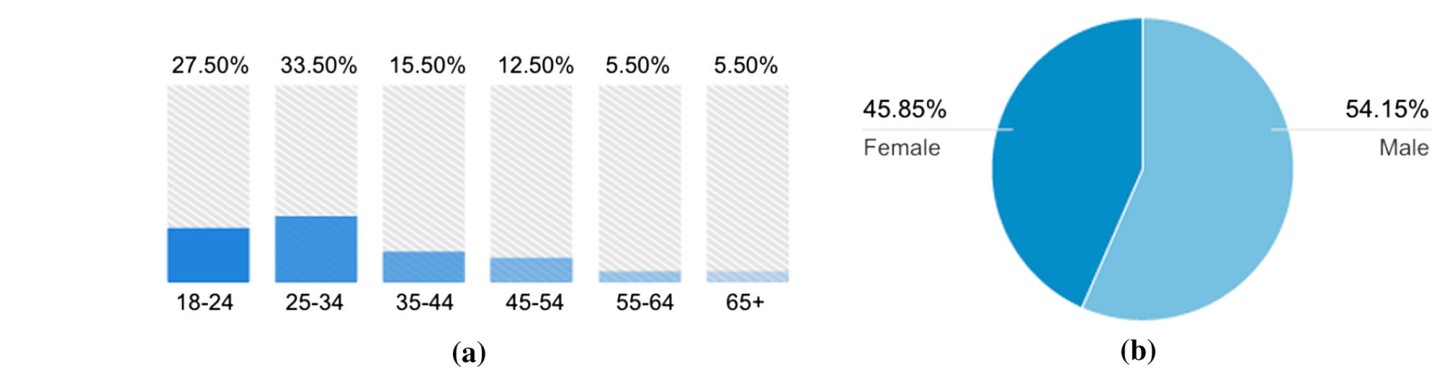
Fig. 9 a Age and b gender distribution of Visual Genome’s crowd workers
图 9 a Visual Genome 众包工人的年龄分布和 b 性别分布
4.2 Region Descriptions
4.2 区域描述
Visual Genome’s main goal is to enable the study of cognitive computer vision tasks. The next step towards understanding images requires studying relationships between objects in scene graph representations of images. However, we observed that collecting scene graphs directly from an image leads to workers annotating easy, frequently-occurring relationships like wearing(man, shirt) instead of focusing on salient parts of the image. This is evident from previous datasets (Johnson et al. 2015; Lu et al. 2016) that contain a large number of such relationships. After experimentation, we observed that when asked to describe an image using natural language, crowd workers naturally start with the most salient part of the image and then move to describing other parts of the image one by one. Inspired by this finding, we focused our attention towards collecting a dataset of region descriptions that is diverse in content.
Visual Genome 的主要目标是推动认知性计算机视觉任务的研究。理解图像的下一步,需要研究图像场景图表示中物体之间的关系。然而我们观察到,如果直接从图像收集场景图,工人往往会标注容易出现、也频繁出现的关系,比如 wearing(man, shirt),而不是把注意力放在图像的显著部分。这一点从包含大量这类关系的先前数据集中也可以看出(Johnson et al. 2015; Lu et al. 2016)。经过试验,我们观察到,当被要求用自然语言描述一幅图时,众包工人会自然地从图像最显著的部分开始,再逐一描写图中的其他部分。受这一发现启发,我们把注意力转向收集内容多样的区域描述数据集。
When a new image is added to the crowdsourcing pipeline with no annotations, it is sent to a worker who is asked to draw three bounding boxes and write three descriptions for the region enclosed by each box. Next, the image is sent to another worker along with the previously written descriptions. Workers are explicitly encouraged to write descriptions that have not been written before. This process is repeated until we have collected 50 region descriptions for each image. To prevent workers from having to skim through a long list of previously written descriptions, we only show them the top seven most similar descriptions. We calculate these most similar descriptions using BLEU-like (Papineni et al. 2002) (n-gram) scores between pairs of sentences. We define the similarity score S between a description and a previous description to be:
当一幅尚无标注的新图进入众包流程时,它会先交给一名工人,要求其画出三个边界框,并为每个框圈出的区域写下三条描述。接下来,这张图连同此前已写的描述一起交给另一名工人。我们明确鼓励工人写出尚未出现过的描述。这一过程重复进行,直到每张图收集到 50 条区域描述。为了避免工人必须浏览一长串已有描述,我们只向他们展示最相似的前七条。我们使用类似 BLEU(Papineni et al. 2002)的(n-gram)分数,在句子对之间计算这些最相似的描述。我们把一条描述 与先前一条描述 之间的相似分数 S 定义为:
$$
\begin{aligned} S_n(d_i, d_j) = b(d_i, d_j) \exp \left( \frac{1}{N}\sum _{n=1}^{N} \log p_n(d_i, d_j)\right) \end{aligned}
$$ (1)
where we enforce a brevity penalty using:
其中我们用下面的方式施加简洁性惩罚:
$$
\begin{aligned} b(d_i, d_j) = \left{ \begin{array}{ll} 1 &{}\quad \hbox {if} ; len(d_i) > len(d_j) \ e^{1-\frac{len(d_j)}{len(d_i)}} &{}\quad \hbox {otherwise} \end{array} \right. \end{aligned}
$$ (2)
and calculates the percentage of n-grams in that match n-grams in .
而 计算的是 中与 的 n-gram 相匹配的 n-gram 比例。
When a worker writes a new description, we programmatically enforce that it has not been repeated by using BLEU score thresholds set to 0.7 to ensure that it is dissimilar to descriptions from both of the following two lists:
当工人写出一条新描述时,我们用程序保证它没有被重复过:把 BLEU 分数阈值设为 0.7,以确保它与下面两个列表中的描述都不相似:
- Image-Specific Descriptions A list of all previously written descriptions for that image.
- 图像特定描述 该图此前已经写过的全部描述列表。
- Global Image Descriptions A list of the top 100 most common written descriptions of all images in the dataset. This prevents very common phrases like “sky is blue” from dominating the set of region descriptions. The list of top 100 global descriptions is continuously updated as more data comes in.
- 全局图像描述 整个数据集中最常见的 100 条已写描述。这样可以避免“sky is blue”这类非常常见的短语占满区域描述。这 100 条全局描述会随着数据增加而持续更新。
Finally, we ask workers to draw bounding boxes that satisfy one requirement: coverage. The bounding box must cover all objects mentioned in the description. Figure 10 shows an example of a good box that covers both the street as well the car mentioned in the description, as well as an example of a bad box.
最后,我们要求工人画出的边界框满足一项要求:覆盖。边界框必须覆盖描述中提到的全部物体。图 10 给出了一个好框的例子,它同时覆盖了描述中提到的 street 和 car,以及一个差框的例子。
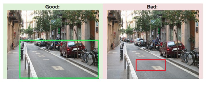
Fig. 10 Good (left) and bad (right) bounding boxes for the phrase “a street with a red car parked on the side,” judged on coverage
图 10 短语“a street with a red car parked on the side”的好(左)与差(右)边界框,按覆盖来评判
4.3 Objects
4.3 物体
Once 50 region descriptions are collected for an image, we extract the visual objects from each description. Each description is sent to one crowd worker, who extracts all the objects from the description and grounds each object as a bounding box in the image. For example, from Fig. 4, let’s consider the description “woman in shorts is standing behind the man.” A worker would extract three objects: woman, shorts, and man. They would then draw a box around each of the objects. We require each bounding box to be drawn to satisfy two requirements: coverage and quality. Coverage has the same definition as described above in Sect. 4.2, where we ask workers to make sure that the bounding box covers the object completely (Fig. 11). Quality requires that each bounding box be as tight as possible around its object such that if the box’s length or height were decreased by one pixel, it would no longer satisfy the coverage requirement. Since a one pixel error can be physically impossible for most workers, we relax the definition of quality to four pixels.
一旦为某张图收集了 50 条区域描述,我们就从每条描述中抽出视觉物体。每条描述会交给一名众包工人,由其从描述中抽出全部物体,并把每个物体作为边界框接地到图像中。例如,从图 4 出发,考虑描述“woman in shorts is standing behind the man。”工人会抽出三个物体:woman、shorts 和 man。然后他们会给每个物体画一个框。我们要求每个边界框的绘制满足两项要求:覆盖和质量。覆盖的定义与上文第 4.2 节相同,即要求工人确保边界框完整覆盖该物体(图 11)。质量要求每个边界框尽量紧贴其物体,以至于如果把框的长度或高度再减少一个像素,它就不再满足覆盖要求。由于对大多数工人来说,一个像素的误差在操作上几乎不可能做到,我们把质量的定义放宽到四个像素。
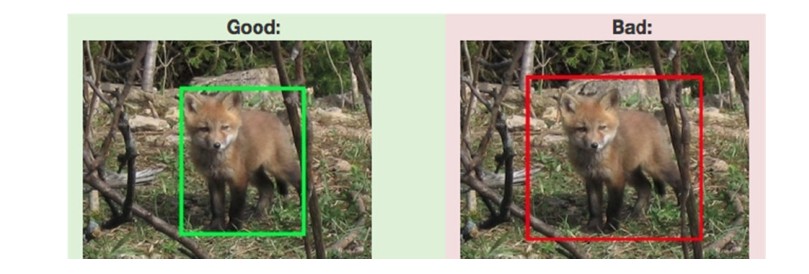
Fig. 11 Good (left) and bad (right) bounding boxes for the object fox, judged on both coverage as well as quality
图 11 物体 fox 的好(左)与差(右)边界框,同时按覆盖和质量来评判
Multiple descriptions for an image might refer to the same object, sometimes with different words. For example, a man in one description might be referred to as person in another description. We can thus use this crowdsourcing stage to build these co-reference chains. With each region description given to a worker to process, we include a list of previously extracted objects as suggestions. This allows a worker to choose a previously drawn box annotated as man instead of redrawing a new box for person.
同一张图的多条描述可能会指同一物体,有时用的词还不同。例如,一条描述中的 man 在另一条描述里可能被称作 person。因此,我们可以利用这一众包阶段来建立这些共指链。在交给工人处理的每条区域描述中,我们附上一份此前已抽出的物体作为建议。这样,工人可以选择一个先前已经画好、并标注为 man 的框,而不必为 person 再画一个新框。
Finally, to increase the speed with which workers complete this task, we also use Stanford’s dependency parser (Manning et al. 2014) to extract nouns automatically and send them to the workers as suggestions. While the parser manages to find most of the nouns, it sometimes misses compound nouns, so we avoided completely depending on this automated method. By combining the parser with crowdsourcing tasks, we were able to speed up our object extraction process without losing accuracy.
最后,为了加快工人完成这项任务的速度,我们还使用斯坦福依存句法分析器(Manning et al. 2014)自动抽出名词,并把它们作为建议发给工人。虽然分析器能够找到大多数名词,但它有时会漏掉复合名词,因此我们避免完全依赖这种自动方法。通过分析器与众包任务相结合,我们在不损失准确率的情况下加快了物体抽取过程。
4.4 Attributes, Relationships, and Region Graphs
4.4 属性、关系与区域图
Once all objects have been extracted from each region description, we can extract the attributes and relationships described in the region. We present each worker with a region description along with its extracted objects and ask them to add attributes to objects or to connect pairs of objects with relationships, based on the text of the description. From the description “woman in shorts is standing behind the man”, workers will extract the attribute standing for the woman and the relationships in(woman, shorts) and behind(woman, man). Together, objects, attributes, and relationships form the region graph for a region description. Some descriptions like “it is a sunny day” do not contain any objects and therefore have no region graphs associated with them. Workers are asked to not generate any graphs for such descriptions. We create scene graphs by combining all the region graphs for an image by combining all the co-referenced objects from different region graphs.
一旦从每条区域描述中抽出了全部物体,我们就可以抽取该区域所描述的属性和关系。我们向每位工人出示一条区域描述及其已抽出的物体,并请他们根据描述文本为物体添加属性,或用关系连接成对的物体。从描述“woman in shorts is standing behind the man”中,工人会为 woman 抽出属性 standing,以及关系 in(woman, shorts) 和 behind(woman, man)。物体、属性和关系合在一起,构成一条区域描述的区域图。像“it is a sunny day”这样的描述不包含任何物体,因此没有与之对应的区域图。我们要求工人不要为这类描述生成任何图。我们通过合并不同区域图中的共指物体,把一张图的全部区域图组合成场景图。
4.5 Scene Graphs
4.5 场景图
The scene graph is the union of all region graphs extracted from region descriptions. We merge nodes from region graphs that correspond to the same object; for example, man and person in two different region graphs might refer to the same object in the image. We say that objects from different graphs refer to the same object if their bounding boxes have an intersection over union of 0.9. However, this heuristic might contain false positives. So, before merging two objects, we ask workers to confirm that a pair of objects with significant overlap are indeed the same object. For example, in Fig. 12 (right), the fox might be extracted from two different region descriptions. These boxes are then combined together (Fig. 12, left) when constructing the scene graph.
场景图是从区域描述中抽出的全部区域图的并集。我们把对应于同一物体的区域图节点合并起来;例如,两张不同区域图中的 man 和 person 可能指的是图像中的同一个物体。如果来自不同图的物体,其边界框的交并比为 0.9,我们就认为它们指的是同一个物体。不过,这一启发式方法可能包含假阳性。因此,在合并两个物体之前,我们会请工人确认一对有显著重叠的物体确实是同一个物体。例如在图 12(右)中,fox 可能从两条不同的区域描述中被抽出。在构建场景图时,这些框会被合并在一起(图 12,左)。
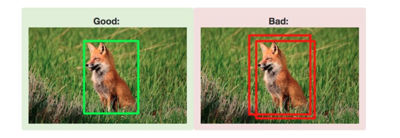
Fig. 12 Each object (fox) has only one bounding box referring to it (left). Multiple boxes drawn for the same object (right) are combined together if they have a minimum threshold of 0.9 intersection over union
图 12 每个物体(fox)只有一个指向它的边界框(左)。为同一物体画出的多个框(右),若交并比达到最低阈值 0.9,就会被合并。
4.6 Questions and Answers
4.6 问题与答案
To create question answer (QA) pairs, we ask the AMT workers to write pairs of questions and answers about an image. To ensure quality, we instruct the workers to follow three rules: 1) start the questions with one of the “six Ws” (who, what, where, when, why and how); 2) avoid ambiguous and speculative questions; 3) be precise and unique, and relate the question to the image such that it is clearly answerable if and only if the image is shown.
为了创建问答(QA)对,我们请 AMT 工人就一幅图像写出成对的问题和答案。为了保证质量,我们要求工人遵守三条规则:1)问题必须以“六个 W”(who、what、where、when、why 和 how)之一开头;2)避免含混和推测性的问题;3)要精确、独特,并把问题与图像关联起来,使得当且仅当出示该图像时,问题才显然可以回答。
We collected two separate types of QAs: freeform QAs and region-based QAs. In freeform QA, we ask a worker to look at an image and write eight QA pairs about it. To encourage diversity, we enforce that workers write at least three different Ws out of the six in their eight pairs. In region-based QA, we ask the workers to write a pair based on a given region. We select the regions that have large areas (more than 5k pixels) and long phrases (more than 4 words). This enables us to collect around twenty region-based pairs at the same cost of the eight freeform QAs. In general, freeform QA tends to yield more diverse QA pairs that enrich the question distribution; region-based QA tends to produce more factual QA pairs at a lower cost.
我们收集了两类不同的问答:自由形式问答和区域问答。在自由形式问答中,我们请一名工人看一张图,并为之写出八对问答。为了鼓励多样性,我们强制要求工人在这八对中至少用到六个 W 里的三种。在区域问答中,我们请工人基于一个给定区域写一对问答。我们选择面积较大(超过 5 千像素)、短语较长(超过 4 个词)的区域。这样,我们就能以与八对自由形式问答相同的成本,收集大约二十对区域问答。总体而言,自由形式问答往往产生更多样的问答对,从而丰富问题分布;区域问答则往往以更低的成本产生更偏事实性的问答对。
4.7 Verification
4.7 核验
All Visual Genome data go through a verification stage as soon as they are annotated. This stage helps eliminate incorrectly labeled objects, attributes, and relationships. It also helps remove region descriptions and questions and answers that might be correct but are vague (“This person seems to enjoy the sun.”), subjective (“room looks dirty”), or opinionated (“Being exposed to hot sun like this may cause cancer”).
Visual Genome 的全部数据在标注完成后会立即进入核验阶段。这一阶段帮助剔除标注错误的物体、属性和关系,也帮助去掉那些或许正确、但含混(“This person seems to enjoy the sun.”)、主观(“room looks dirty”)或带有观点(“Being exposed to hot sun like this may cause cancer”)的区域描述和问答。
Verification is conducted using two separate strategies: majority voting (Snow et al. 2008) and rapid judgments (Krishna et al. 2016). All components of the dataset except objects are verified using majority voting. Majority voting(Snow et al. 2008) involves three unique workers looking at each annotation and voting on whether it is factually correct. An annotation is added to our dataset if at least two (a majority) out of the three workers verify that it is correct.
核验采用两种不同策略:多数投票(Snow et al. 2008)和快速判断(Krishna et al. 2016)。数据集中除物体以外的所有部分都用多数投票核验。多数投票(Snow et al. 2008)由三名不同的工人查看每条标注,并对其是否事实正确进行投票。如果至少两名(多数)工人确认某条标注正确,该标注就会被加入我们的数据集。
We only use rapid judgments to speed up the verification of the objects in our dataset. Rapid judgments (Krishna et al. 2016) use an interface inspired by rapid serial visual processing that enable verification of objects with an order of magnitude increase in speed than majority voting.
我们只使用快速判断来加快数据集中物体的核验。快速判断(Krishna et al. 2016)采用一种受快速序列视觉呈现启发的界面,使物体核验的速度比多数投票高出一个数量级。
4.8 Canonicalization
4.8 规范化
All the descriptions and QAs that we collect are freeform worker-generated texts. They are not constrained by any limitations. For example, we do not force workers to refer to a man in the image as a man. We allow them to choose to refer to the man as person, boy, man, etc. This ambiguity makes it difficult to collect all instances of man from our dataset. In order to reduce the ambiguity in the concepts of our dataset and connect it to other resources used by the research community, we map all objects, attributes, relationships, and noun phrases in region descriptions and QAs to synsets in WordNet (Miller 1995). In the example above, person, boy, and man would map to the synsets: person.n.01 (a human being), male_child.n.01 (a youthful male person) and man.n.03 (the generic use of the word to refer to any human being) respectively. Thanks to the WordNet hierarchy it is now possible to fuse those three expressions of the same concept into person.n.01 (a human being), which is the lowest common ancestor node of all aforementioned synsets.
我们收集的全部描述和问答都是工人写出的自由文本,不受任何限制约束。例如,我们并不强迫工人把图中的一个男人称作 man。我们允许他们选择用 person、boy、man 等来指称这个人。这种歧义使得很难从我们的数据集中收集 man 的全部实例。为了降低数据集概念中的歧义,并把它与研究社区使用的其他资源连接起来,我们把所有物体、属性、关系,以及区域描述和问答中的名词短语,都映射到 WordNet(Miller 1995)中的同义词集。在上面的例子中,person、boy 和 man 会分别映射到同义词集:person.n.01 (a human being)、male_child.n.01 (a youthful male person) 和 man.n.03 (the generic use of the word to refer to any human being)。多亏有 WordNet 的层次结构,现在可以把这三种对同一概念的表达归并到 person.n.01 (a human being),它是上述同义词集的最低共同祖先节点。
We use the Stanford NLP tools (Manning et al. 2014) to extract the noun phrases from the region descriptions and QAs. Next, we map them to their most frequent matching synset in WordNet according to WordNet lexeme counts. We then refine this simple heuristic by hand-crafting mapping rules for the 30 most common failure cases. For example according to WordNet’s lexeme counts the most common semantic for “table” is table.n.01 (a set of data arranged in rows and columns). However in our data it is more likely to see pieces of furniture and therefore bias the mapping towards table.n.02 (a piece of furniture having a smooth flat top that is usually supported by one or more vertical legs). The objects in our scene graphs are already noun phrases and are mapped to WordNet in the same way.
我们使用斯坦福自然语言处理工具(Manning et al. 2014)从区域描述和问答中抽出名词短语。接下来,我们按 WordNet 词位计数,把它们映射到其中最频繁匹配的同义词集。然后,我们为最常见的 30 种失败情形手工制定映射规则,来改进这一简单启发式方法。例如,按 WordNet 的词位计数,“table”最常见的语义是 table.n.01 (a set of data arranged in rows and columns)。但在我们的数据里,更常见的是家具,因此会把映射偏向 table.n.02 (a piece of furniture having a smooth flat top that is usually supported by one or more vertical legs)。我们场景图中的物体已经是名词短语,并以同样的方式映射到 WordNet。
We normalize each attribute based on morphology (so called “stemming”) and map them to the WordNet adjectives. We include 15 hand-crafted rules to address common failure cases, which typically occur when the concrete or spatial sense of the word seen in an image is not the most common overall sense. For example, the synset long.a.02 (of relatively great or greater than average spatial extension) is less common in WordNet than long.a.01 (indicating a relatively great or greater than average duration of time), even though instances of the word “long” in our images are much more likely to refer to that spatial sense.
我们基于形态(所谓“词干提取”)对每个属性做规范化,并把它们映射到 WordNet 形容词。我们加入了 15 条手工规则,以处理常见的失败情形;这些情形通常出现在图像中看到的具体或空间义项并不是该词总体上最常见义项的时候。例如,同义词集 long.a.02 (of relatively great or greater than average spatial extension) 在 WordNet 中不如 long.a.01 (indicating a relatively great or greater than average duration of time) 常见,尽管我们图像中“long”一词的实例更可能指那个空间义项。
For relationships, we ignore all prepositions as they are not recognized by WordNet. Since the meanings of verbs are highly dependent upon their morphology and syntactic placement (e.g. passive cases, prepositional phrases), we try to find WordNet synsets whose sentence frames match with the context of the relationship. Sentence frames in WordNet are formalized syntactic frames in which a certain sense of a word might appear; e.g., play.v.01: participate in games or sport occurs in the sentence frames “Somebody [play]s” and “Somebody [play]s something.” For each verb-synset pair, we then consider the root hypernym of that synset to reduce potential noise from WordNet’s fine-grained sense distinctions. The WordNet hierarchy for verbs is segmented and originates from over 100 root verbs. For example, draw.v.01: cause to move by pulling traces back to the root hypernym move.v.02: cause to move or shift into a new position, while draw.v.02: get or derive traces to the root get.v.01: come into the possession of something concrete or abstract. We also include 20 hand-mapped rules, again to correct for WordNet’s lower representation of concrete or spatial senses.
对于关系,我们忽略所有介词,因为 WordNet 并不识别它们。由于动词的意义高度依赖于其形态和句法位置(例如被动情形、介词短语),我们试图寻找句子框架与该关系上下文相匹配的 WordNet 同义词集。WordNet 中的句子框架是形式化的句法框架,某个词的特定义项可能出现在其中;例如,play.v.01: participate in games or sport 出现在句子框架“Somebody [play]s”和“Somebody [play]s something.”中。对每一对动词–同义词集,我们再考虑该同义词集的根上位词,以降低 WordNet 细粒度义项区分可能带来的噪声。WordNet 中动词的层次是分段的,源自 100 多个根动词。例如,draw.v.01: cause to move by pulling 可以追溯到根上位词 move.v.02: cause to move or shift into a new position,而 draw.v.02: get or derive 则追溯到根词 get.v.01: come into the possession of something concrete or abstract。我们还加入了 20 条手工映射规则,同样是为了纠正 WordNet 对具体或空间义项表征不足的问题。
These mappings are not perfect and still contain some ambiguity. Therefore, we send all our mappings along with the top four alternative synsets for each term to AMT. We ask workers to verify that our mapping was accurate and change the mapping to an alternative one if it was a better fit. We present workers with the concept we want to canonicalize along with our proposed corresponding synset with 4 additional options. To prevent workers from always defaulting to the our proposed synset, we do not explicitly specify which one of the 5 synsets presented is our proposed synset. Section 5.8 provides experimental precision and recall scores for our canonicalization strategy.
这些映射并不完美,仍然含有一些歧义。因此,我们把全部映射以及每个术语的前四个备选同义词集一起发给 AMT。我们请工人核验我们的映射是否准确,如果有更合适的备选,就把映射改过去。我们向工人出示想要规范化的概念,以及我们提议的对应同义词集,外加 4 个选项。为了防止工人总是默认选择我们提议的同义词集,我们并不明确指出所出示的 5 个同义词集中哪一个是我们提议的。第 5.8 节给出了我们规范化策略的实验精确率和召回率。
5 Dataset Statistics and Analysis
5 数据集统计与分析
In this section, we provide statistical insights and analysis for each component of Visual Genome. Specifically, we examine the distribution of images (Sect. 5.1) and the collected data for region descriptions (Sect. 5.2) and questions and answers (Sect. 5.7). We analyze region graphs and scene graphs together in one section (Sect. 5.6), but we also break up these graph structures into their three constituent parts—objects (Sect. 5.3), attributes (Sect. 5.4), and relationships (Sect. 5.5)—and study each part individually. Finally, we describe our canonicalization pipeline and results (Sect. 5.8).
本节给出 Visual Genome 各个组成部分的统计洞察与分析。具体而言,我们考察图像(第 5.1 节)的分布,以及为区域描述(第 5.2 节)和问答(第 5.7 节)收集到的数据。我们在同一节中一起分析区域图和场景图(第 5.6 节),但也会把这些图结构拆成三个构成部分——物体(第 5.3 节)、属性(第 5.4 节)和关系(第 5.5 节)——并分别研究每一部分。最后,我们说明规范化流程和结果(第 5.8 节)。
5.1 Image Selection
5.1 图像选取
The Visual Genome dataset consists of all creative commons images from the intersection of MS-COCO’s (Lin et al. 2014) 328, 000 images and YFCC100M’s (Thomee et al. 2016) 100 million images. This allows Visual Genome annotations to be utilized together with the YFCC tags and MS-COCO’s segmentations and full image captions. These images are real-world, non-iconic images that were uploaded onto Flickr by users. The images range from as small as 72 pixels wide to as large as 1280 pixels wide, with an average width of 500 pixels. We collected the WordNet synsets into which our images can be categorized using the same method as ImageNet (Deng et al. 2009). Visual Genome images can be categorized into 972 ImageNet synsets. Note that objects, attributes and relationships are categorized separately into more than 18K WordNet synsets (Sect. 5.8). Figure 13 shows the top synsets to which our images belong. “ski” is the most common synset, with 2612 images; it is followed by “ballplayer” and “racket,” with all three synsets referring to images of people playing sports. Our dataset is somewhat biased towards images of people, as Fig. 13 shows; however, they are quite diverse overall, as the top 25 synsets each have over 800 images, while the top 50 synsets each have over 500 examples.
Visual Genome 数据集由 MS-COCO(Lin et al. 2014)的 328,000 张图像与 YFCC100M(Thomee et al. 2016)的 1 亿张图像交集中、全部 张知识共享协议图像组成。这样,Visual Genome 的标注就可以与 YFCC 标签以及 MS-COCO 的分割和整图配文一起使用。这些图像是用户上传到 Flickr 上的真实世界、非典型图像。图像宽度从最小 72 像素到最大 1280 像素,平均宽度为 500 像素。我们用与 ImageNet(Deng et al. 2009)相同的方法,收集了可以把我们这 张图像归入其中的 WordNet 同义词集。Visual Genome 的图像可以归入 972 个 ImageNet 同义词集。需要注意,物体、属性和关系被另行归入 1.8 万多个 WordNet 同义词集(第 5.8 节)。图 13 显示了我们的图像所属的排名靠前的同义词集。“ski”是最常见的同义词集,有 2612 张图;其后是“ballplayer”和“racket”,这三个同义词集都指向人们进行体育运动的图像。如图 13 所示,我们的数据集在人物图像上有一定偏向;不过总体仍然相当多样,因为前 25 个同义词集各自都有超过 800 张图,前 50 个同义词集各自都有超过 500 个例子。
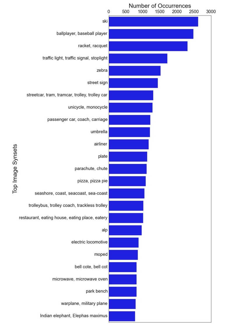
Fig. 13 A distribution of the top 25 image synsets in the Visual Genome dataset. A variety of synsets are well represented in the dataset, with the top 25 synsets having at least 800 example images each. Note that an image synset is the label of the entire image according to the ImageNet ontology and are separate from the synsets for objects, attributes and relationships
图 13 Visual Genome 数据集中排名前 25 的图像同义词集分布。数据集中各类同义词集都有较好代表,前 25 个同义词集各自至少有 800 张示例图像。需要注意,图像同义词集是整张图按 ImageNet 本体给出的标签,与物体、属性和关系的同义词集是分开的。
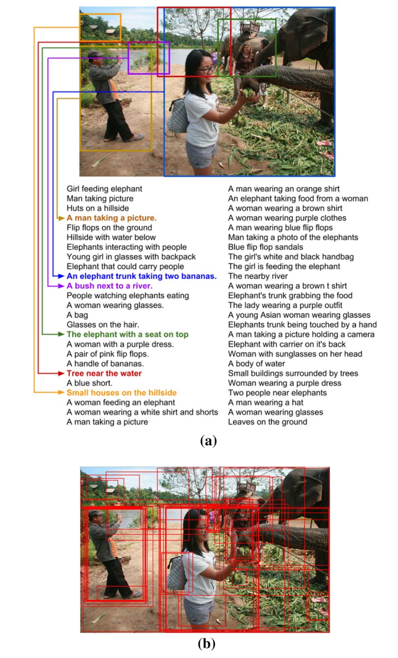
Fig. 14 a An example image from the dataset with its region descriptions. We only display localizations for 6 of the descriptions to avoid clutter; all descriptions do have corresponding bounding boxes. b All region bounding boxes visualized on the image
图 14 a 数据集中的一张示例图像及其区域描述。为避免杂乱,我们只显示 条描述中 6 条的定位;全部 条描述都有对应的边界框。b 在图像上可视化全部 个区域边界框。
5.2 Region Description Statistics
5.2 区域描述统计
One of the primary components of Visual Genome is its region descriptions. Every image includes an average of regions with a bounding box and a descriptive phrase. Figure 14 shows an example image from our dataset with its 50 region descriptions. We display bounding boxes for only 6 out of the 50 descriptions in the figure to avoid clutter. These descriptions tend to be highly diverse and can focus on a single object, like in “A bag,” or on multiple objects, like in “Man taking a photo of the elephants.” They encompass the most salient parts of the image, as in “An elephant taking food from a woman,” while also capturing the background, as in “Small buildings surrounded by trees.”
Visual Genome 的主要组成部分之一是区域描述。每张图平均包含 个带边界框和描述短语的区域。图 14 给出了我们数据集中的一张示例图像及其 50 条区域描述。为避免杂乱,图中只显示了 50 条描述中 6 条的边界框。这些描述往往高度多样,既可以聚焦于单个物体,如“A bag”,也可以聚焦于多个物体,如“Man taking a photo of the elephants.”它们既涵盖图像中最显著的部分,如“An elephant taking food from a woman”,也捕捉背景,如“Small buildings surrounded by trees.”
MS-COCO (Lin et al. 2014) dataset is good at generating variations on a single scene-level descriptor. Consider three sentences from MS-COCO dataset on a similar image: “there is a person petting a very large elephant,” “a person touching an elephant in front of a wall,” and “a man in white shirt petting the cheek of an elephant.” These three sentences are single scene-level descriptions. In comparison, Visual Genome descriptions emphasize different regions in the image and thus are less semantically similar. To ensure diversity in the descriptions, we use BLEU score (Papineni et al. 2002) thresholds between new descriptions and all previously written descriptions. More information about crowdsourcing can be found in Sect. 4.
MS-COCO(Lin et al. 2014)数据集擅长围绕同一条场景级描述生成变体。考虑 MS-COCO 数据集中一张类似图像上的三句话:“there is a person petting a very large elephant”、“a person touching an elephant in front of a wall”和“a man in white shirt petting the cheek of an elephant。”这三句都是单句的场景级描述。相比之下,Visual Genome 的描述强调图像中的不同区域,因而在语义上不那么相似。为了保证描述的多样性,我们在新描述与此前所有已写描述之间使用 BLEU 分数(Papineni et al. 2002)阈值。更多关于众包的信息见第 4 节。
Region descriptions must be specific enough in an image to describe individual objects (e.g. “A bag”), but they must also be general enough to describe high-level concepts in an image (e.g. “A man being chased by a bear”). Qualitatively, we note that regions that cover large portions of the image tend to be general descriptions of an image, while regions that cover only a small fraction of the image tend to be more specific. In Fig. 15a, we show the distribution of regions over the width of the region normalized by the width of the image. We see that the majority of our regions tend to be around 10 to of the image width. We also note that there are a large number of regions covering of the image width. These regions usually include elements like “sky,” “ocean,” “snow,” “mountains,” etc. that cannot be bounded and thus span the entire image width. In Fig. 15b, we show a similar distribution over the normalized height of the region. We see a similar overall pattern, as most of our regions tend to be very specific descriptions of about to of the image height. Unlike the distribution over width, however, we do not see a increase in the number of regions that span the entire height of the image, as there are no common visual equivalents that span images vertically. Out of all the descriptions gathered, only one or two of them tend to be global scene descriptions that are similar to MS-COCO (Lin et al. 2014) (Fig. 17).
区域描述必须足够具体,以便描写图中的个别物体(如“A bag”),又必须足够概括,以便描写图中的高层概念(如“A man being chased by a bear”)。从定性上看,我们注意到,覆盖图像较大部分的区域往往是对图像的一般性描述,而只覆盖图像一小部分的区域往往更具体。在图 15a 中,我们给出区域宽度除以图像宽度后的区域分布。可以看到,我们的大多数区域大约占图像宽度的 10% 到 。我们也注意到,有大量区域覆盖了图像宽度的 。这些区域通常包括“sky”、“ocean”、“snow”、“mountains”等无法被框住、因而横跨整个图像宽度的元素。在图 15b 中,我们给出区域高度归一化后的类似分布。总体模式相似,因为我们的大多数区域都是约占图像高度 到 的非常具体的描述。不过,与宽度上的分布不同,我们没有看到横跨图像整个高度的区域数量增加,因为并不存在常见的、在垂直方向上贯穿图像的视觉对应物。在收集到的全部描述中,通常只有一两句是与 MS-COCO(Lin et al. 2014)类似的全局场景描述(图 17)。
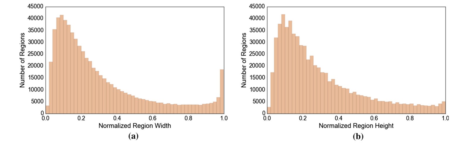
Fig. 15 a A distribution of the width of the bounding box of a region description normalized by the image width. b A distribution of the height of the bounding box of a region description normalized by the image height
图 15 a 区域描述边界框宽度除以图像宽度后的分布。b 区域描述边界框高度除以图像高度后的分布。
In Fig. 16, we show the distribution of the length (word count) of these region descriptions. The average word count for a description is 5 words, with a minimum of 1 and a maximum of 12 words. In Fig. 18a, we plot the most common phrases occurring in our region descriptions, with common stop words removed. Common visual elements like “green grass,” “tree [in] distance,” and “blue sky” occur much more often than other, more nuanced elements like “fresh strawberry.” We also study descriptions with finer precision in Fig. 18b, where we plot the most common words used in descriptions. Again, we eliminate stop words from our study. Colors like “white” and “black” are the most frequently used words to describe visual concepts; we conduct a similar study on other captioning datasets including MS-COCO (Lin et al. 2014) and Flickr 30K (Young et al. 2014) and find a similar distribution with colors occurring most frequently. Besides colors, we also see frequent occurrences of common objects like “man” and “tree” and of universal visual elements like “sky.”
在图 16 中,我们给出这些区域描述的长度(词数)分布。一条描述的平均词数是 5,最少 1 个词,最多 12 个词。在图 18a 中,我们画出区域描述中最常见的短语,并去掉了常见停用词。“green grass”、“tree [in] distance”和“blue sky”这类常见视觉元素,出现频率远高于“fresh strawberry”这类更细致的元素。我们还在图 18b 中以更细的精度研究描述,画出描述中最常用的词。同样,我们在分析中去掉了停用词。像“white”和“black”这样的颜色,是用来描述视觉概念时最频繁使用的词;我们也对包括 MS-COCO(Lin et al. 2014)和 Flickr 30K(Young et al. 2014)在内的其他配文数据集做了类似研究,发现分布相似,颜色出现得最频繁。除颜色之外,我们还看到“man”和“tree”这类常见物体,以及“sky”这类普遍视觉元素频繁出现。
Semantic Diversity We also study the actual semantic contents of the descriptions. We use an unsupervised approach to analyze the semantics of these descriptions. Specifically, we use word2vec’s (Mikolov et al. 2013) pre-trained model on Google news corpus to convert each word in a description to a 300-dimensional vector. Next, we remove stop words and average the remaining words to get a vector representation of the whole region description. This pipeline is outlined in Fig. 17. We use hierarchical agglomerative clustering (Steinbach et al. 2000) on vector representations of each region description and find 71 semantic and syntactic groupings or “clusters.” Figure 19a shows four such example clusters. One cluster contains all descriptions related to tennis, like “A man swings the racquet” and “White lines on the ground of the tennis court,” while another cluster contains descriptions related to numbers, like “Three dogs on the street” and “Two people inside the tent.” To quantitatively measure the diversity of Visual Genome’s region descriptions, we calculate the number of clusters represented in a single image’s region descriptions. We show the distribution of the variety of descriptions for an image in Fig. 19b. We find that on average, each image contains descriptions from 17 different clusters. The image with the least diverse descriptions contains descriptions from 4 clusters, while the image with the most diverse descriptions contains descriptions from 26 clusters.
语义多样性 我们也研究这些描述的实际语义内容。我们用一种无监督方法来分析这些描述的语义。具体而言,我们使用在谷歌新闻语料上预训练的 word2vec(Mikolov et al. 2013)模型,把描述中的每个词转换成 300 维向量。接下来,我们去掉停用词,并对剩余的词取平均,得到整条区域描述的向量表示。这一流程概括在图 17 中。我们对每条区域描述的向量表示做层次凝聚聚类(Steinbach et al. 2000),得到 71 个语义和句法分组,或称“簇”。图 19a 展示了其中四个簇。一个簇包含与网球相关的全部描述,如“A man swings the racquet”和“White lines on the ground of the tennis court”,另一个簇则包含与数字相关的描述,如“Three dogs on the street”和“Two people inside the tent。”为了定量衡量 Visual Genome 区域描述的多样性,我们计算单张图的区域描述中出现了多少个簇。我们在图 19b 中给出一幅图的描述多样性分布。我们发现,平均每张图的描述来自 17 个不同的簇。描述最不多样的图像来自 4 个簇,描述最多样的图像来自 26 个簇。
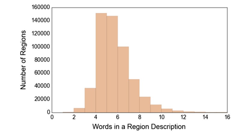
Fig. 16 A distribution of the number of words in a region description. The average number of words in a region description is 5, with shortest descriptions of 1 word and longest descriptions of 16 words
图 16 一条区域描述中的词数分布。区域描述的平均词数是 5,最短为 1 个词,最长为 16 个词。
Finally, we also compare the descriptions in Visual Genome to the captions in MS-COCO. First we aggregate all Visual Genome and MS-COCO descriptions and remove all stop words. After removing stop words, the descriptions from both datasets are roughly the same length. We conduct a similar study, in which we vectorize the descriptions for each image and calculate each dataset’s cluster diversity per image. We find that on average, 2 clusters are represented in the captions for each image in MS-COCO, with very few images in which 5 clusters are represented. Because each image in MS-COCO only contains 5 captions, it is not a fair comparison to compare the number of clusters represented in all the region descriptions in the Visual Genome dataset. We thus randomly sample 5 Visual Genome region descriptions per image and calculate the number of clusters in an image. We find that Visual Genome descriptions come from 4 or 5 clusters. We show our comparison results in Fig. 19c. The difference between the semantic diversity between the two datasets is statistically significant (, ) (Fig. 20).
最后,我们还将 Visual Genome 中的描述与 MS-COCO 中的配文相比较。我们先汇总全部 Visual Genome 和 MS-COCO 描述并去掉所有停用词。去掉停用词后,两个数据集的描述长度大致相同。我们做了类似的研究:把每张图的描述向量化,并计算每个数据集每张图的簇多样性。我们发现,MS-COCO 中每张图的配文平均来自 2 个簇,很少有图像覆盖到 5 个簇。因为 MS-COCO 中每张图只有 5 条配文,拿 Visual Genome 中一张图的全部区域描述所覆盖的簇数来比较并不公平。因此,我们从每张 Visual Genome 图像中随机抽取 5 条区域描述,再计算一张图中的簇数。我们发现,Visual Genome 的描述来自 4 或 5 个簇。比较结果见图 19c。两个数据集在语义多样性上的差异具有统计显著性(,)(图 20)。
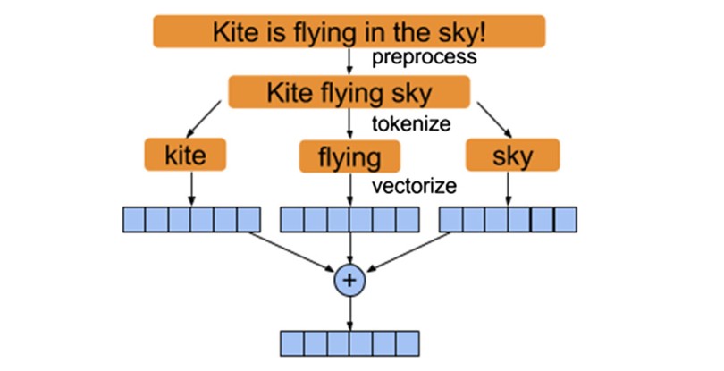
Fig. 17 The process used to convert a region description into a 300-dimensional vectorized representation
图 17 把一条区域描述转换成 300 维向量表示所用的流程
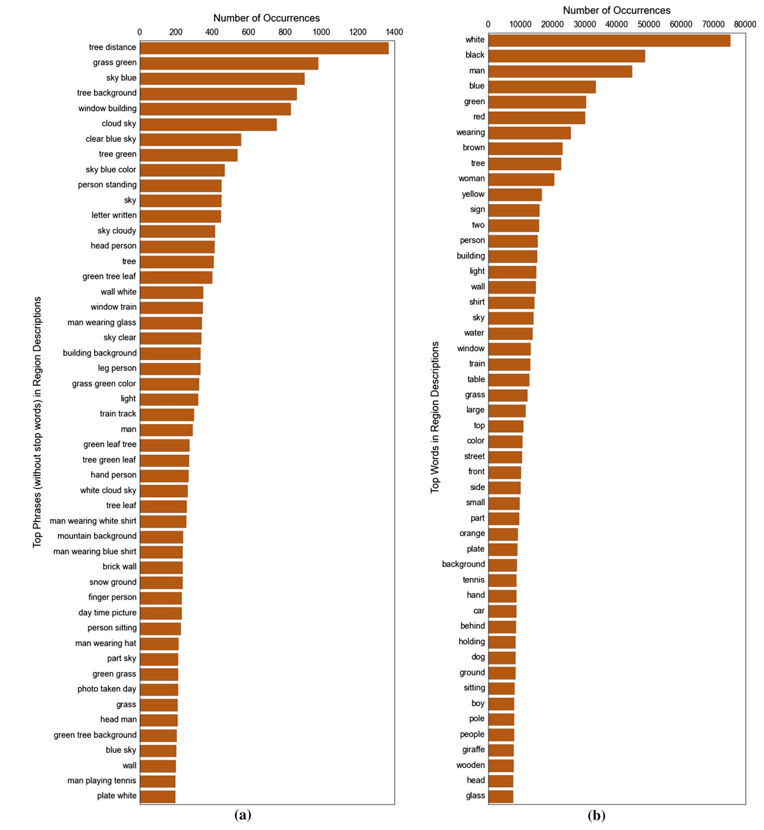
Fig. 18 a A plot of the most common visual concepts or phrases that occur in region descriptions. The most common phrases refer to universal visual concepts like “blue sky,” “green grass,” etc. b A plot of the most frequently used words in region descriptions. Each word is treated as an individual token regardless of which region description it came from. Colors occur the most frequently, followed by common objects like man and dog and universal visual concepts like “sky”
图 18 a 区域描述中最常见的视觉概念或短语。最常见的短语指向普遍的视觉概念,如“blue sky”、“green grass”等。b 区域描述中最常使用的词。每个词都当作独立记号,不论它来自哪一条区域描述。颜色出现得最频繁,其次是 man 和 dog 这类常见物体,以及“sky”这类普遍视觉概念。
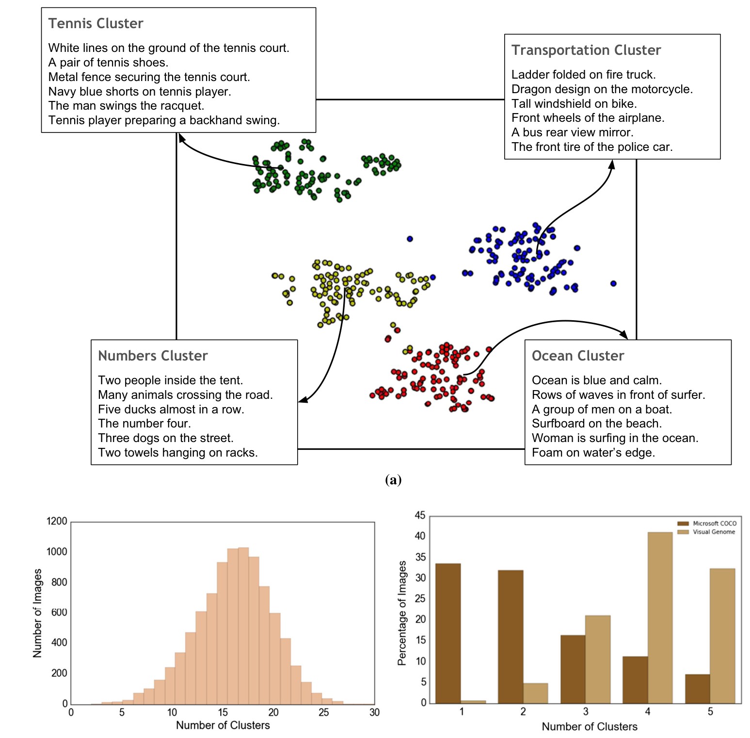
Fig. 19 a Example illustration showing four clusters of region descriptions and their overall themes. Other clusters not shown due to limited space. b Distribution of images over number of clusters represented in each image’s region descriptions. c We take Visual Genome with 5 random descriptions taken from each image and MS-COCO dataset with all 5 sentence descriptions per image and compare how many clusters are represented in the descriptions. We show that Visual Genome’s descriptions are more varied for a given image, with an average of 4 clusters per image, while MS-COCO’s images have an average of 2 clusters per image
图 19 a 示例图示,给出四个区域描述簇及其总体主题。其余簇因篇幅所限未画出。b 图像按其区域描述所覆盖的簇数分布。c 我们从 Visual Genome 每张图中随机取 5 条描述,并与 MS-COCO 数据集中每张图全部 5 句描述相比较,看这些描述覆盖了多少个簇。结果表明,就给定图像而言,Visual Genome 的描述更多样,平均每张图覆盖 4 个簇,而 MS-COCO 的图像平均覆盖 2 个簇。
Table 3 Comparison of Visual Genome objects and categories to related datasets
| Visual Genome | ILSVRC det. (Russakovsky et al. 2015) | MS-COCO (Lin et al. 2014) | Caltech101 (Fei-Fei et al. 2007) | Caltech256 (Griffin et al. 2007) | PASCAL det. (Everingham et al. 2010) | Abstract scenes (Zitnick and Parikh 2013) | |
|---|---|---|---|---|---|---|---|
| Images | 108,077 | 476,688 | 328,000 | 9144 | 30,608 | 11,530 | 10,020 |
| Total objects | 3,843,636 | 534,309 | 2,500,000 | 9144 | 30,608 | 27,450 | 58 |
| Total categories | 33,877 | 200 | 80 | 102 | 257 | 20 | 11 |
| Objects per category | 113.45 | 2671.50 | 27472.50 | 90 | 119 | 1372.50 | 5.27 |
表 3 Visual Genome 的物体与类别同相关数据集的比较
| Visual Genome | ILSVRC det. (Russakovsky et al. 2015) | MS-COCO (Lin et al. 2014) | Caltech101 (Fei-Fei et al. 2007) | Caltech256 (Griffin et al. 2007) | PASCAL det. (Everingham et al. 2010) | Abstract scenes (Zitnick and Parikh 2013) | |
|---|---|---|---|---|---|---|---|
| 图像数 | 108,077 | 476,688 | 328,000 | 9144 | 30,608 | 11,530 | 10,020 |
| 物体总数 | 3,843,636 | 534,309 | 2,500,000 | 9144 | 30,608 | 27,450 | 58 |
| 类别总数 | 33,877 | 200 | 80 | 102 | 257 | 20 | 11 |
| 每类别物体数 | 113.45 | 2671.50 | 27472.50 | 90 | 119 | 1372.50 | 5.27 |
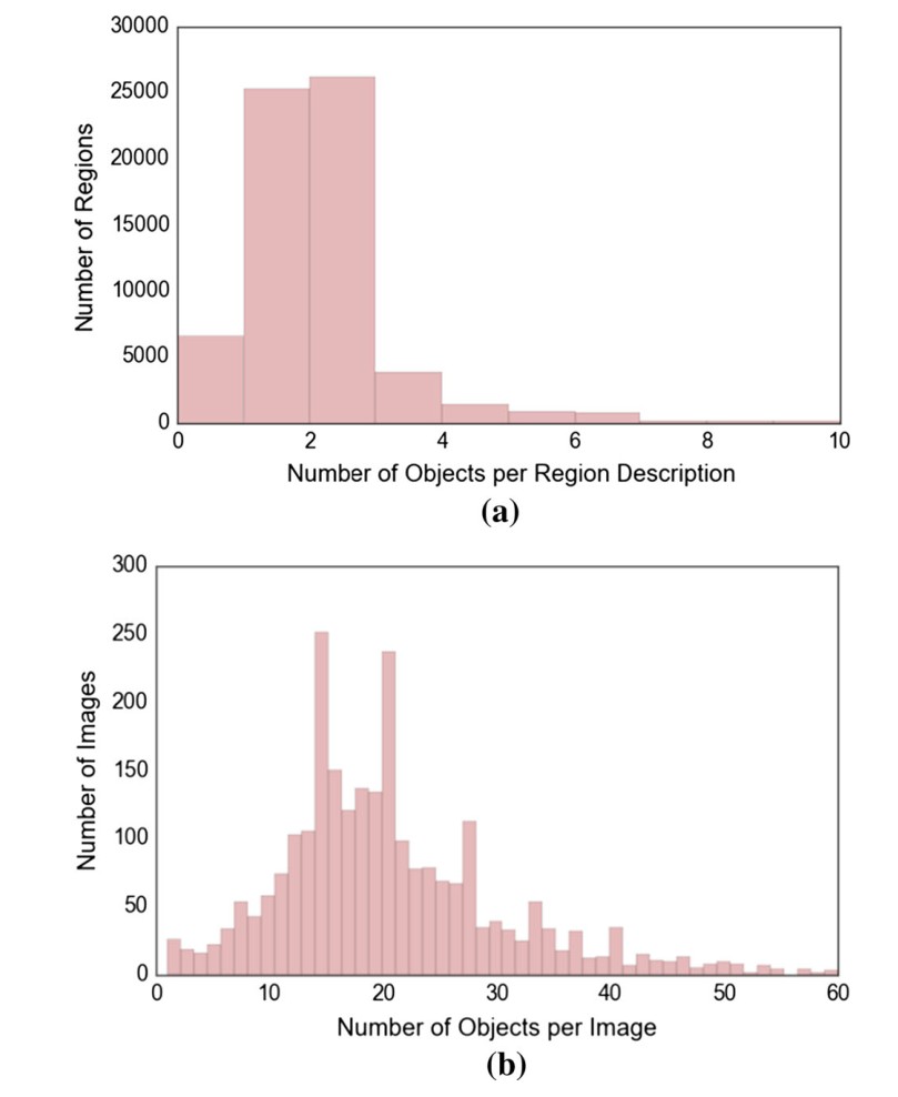
Fig. 20 a Distribution of the number of objects per region. Most regions have between 0 and 2 objects. b Distribution of the number of objects per image. Most images contain between 15 and 20 objects
图 20 a 每个区域中的物体数分布。大多数区域有 0 到 2 个物体。b 每张图中的物体数分布。大多数图像包含 15 到 20 个物体。
5.3 Object Statistics
5.3 物体统计
In comparison to related datasets, Visual Genome fares well in terms of object density and diversity (Table 3). Visual Genome contains approximately objects per image, exceeding ImageNet (Deng et al. 2009), PASCAL (Everingham et al. 2010), MS-COCO (Lin et al. 2014), and other datasets by large margins. As shown in Fig. 21, there are more object categories represented in Visual Genome than in any other dataset. This comparison is especially pertinent with regards to Microsoft MS-COCO (Lin et al. 2014), which uses the same images as Visual Genome. The lower count of objects per category is a result of our higher number of categories. For a fairer comparison with ILSVRC 2014 Detection (Russakovsky et al. 2015), Visual Genome has about 2239 objects per category when only the top 200 categories are considered, which is comparable to ILSVRC’s 2671.5 objects per category. For a fairer comparison with MS-COCO, Visual Genome has about 3768 objects per category when only the top 80 categories are considered. This is comparable to MS-COCO’s (Lin et al. 2014) object distribution.
与相关数据集相比,Visual Genome 在物体密度和多样性方面表现很好(表 3)。Visual Genome 大约每张图有 个物体,大幅度超过 ImageNet(Deng et al. 2009)、PASCAL(Everingham et al. 2010)、MS-COCO(Lin et al. 2014)以及其他数据集。如图 21 所示,Visual Genome 中表示出的物体类别比任何其他数据集都多。这一比较对同样使用 Visual Genome 所用图像的 Microsoft MS-COCO(Lin et al. 2014)尤其贴切。每类别物体数较低,是我们类别数更多的结果。为了与 ILSVRC 2014 Detection(Russakovsky et al. 2015)更公平地比较,如果只考虑排名前 200 的类别,Visual Genome 大约每个类别有 2239 个物体,与 ILSVRC 每个类别 2671.5 个物体相当。为了与 MS-COCO 更公平地比较,如果只考虑排名前 80 的类别,Visual Genome 大约每个类别有 3768 个物体。这与 MS-COCO(Lin et al. 2014)的物体分布相当。
The objects in Visual Genome come from a variety of categories. As shown in Fig. 22 (b), objects related to WordNet categories such as humans, animals, sports, and scenery are most common; this is consistent with the general bias in image subject matter in our dataset. Common objects like man, person, and woman occur especially frequently with occurrences of 24K, 17K, and 11K. Other objects that also occur in MS-COCO (Lin et al. 2014) are also well represented with around 5000 instances on average. Figure 22a shows some examples of objects in images. Objects in Visual Genome span a diverse set of Wordnet categories like food, animals, and man-made structures.
Visual Genome 中的 个物体来自多种类别。如图 22(b)所示,与人、动物、运动和风景等 WordNet 类别相关的物体最为常见;这与我们数据集在图像主题上的总体偏向一致。man、person 和 woman 这类常见物体出现得尤其频繁,分别出现 2.4 万、1.7 万和 1.1 万次。在 MS-COCO(Lin et al. 2014)中也出现的其他物体也有较好代表,平均大约有 5000 个实例。图 22a 给出了图像中的一些物体例子。Visual Genome 中的物体覆盖了食物、动物和人造结构等多样的 WordNet 类别。
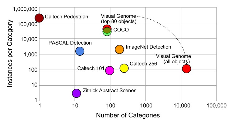
Fig. 21 Comparison of object diversity between various datasets. Visual Genome far surpasses other datasets in terms of number of categories. When considering only the top 80 object categories, it contains a comparable number of objects as MS-COCO. The dashed line is a visual aid connecting the two Visual Genome data points
图 21 各数据集物体多样性的比较。就类别数而言,Visual Genome 远远超过其他数据集。如果只看排名前 80 的物体类别,它包含的物体数量与 MS-COCO 相当。虚线只是连接 Visual Genome 两个数据点的视觉辅助。
It is important to look not only at what types of objects we have but also at the distribution of objects in images and regions. Figure 20a shows, as expected, that we have between 0 and 2 objects in each region on average. It is possible for regions to contain no objects if their descriptions refer to no explicit objects in the image. For example, a region described as “it is dark outside” has no objects to extract. Regions with only one object generally have descriptions that focus on the attributes of a single object. On the other hand, regions with two or more objects generally have descriptions that contain both attributes of specific objects and relationships between pairs of objects.
不仅要看我们有哪些类型的物体,还要看物体在图像和区域中的分布,这一点很重要。图 20a 显示,正如所预期的,每个区域平均有 0 到 2 个物体。如果区域的描述并未提及图中的明确物体,该区域就可能不含物体。例如,被描述为“it is dark outside”的区域没有可抽出的物体。只含一个物体的区域,其描述一般聚焦于单个物体的属性。另一方面,含有两个或更多物体的区域,其描述通常既包含特定物体的属性,也包含成对物体之间的关系。
As shown in Fig. 20b, each image contains on average around distinct objects. Few images have an extremely high number of objects (e.g. over 40). Due to the image biases that exist in the dataset, we have twice as many annotations for men than we do of women.
如图 20b 所示,每张图平均包含大约 个不同的物体。很少有图像拥有极高的物体数(例如超过 40 个)。由于数据集中存在的图像偏向,我们对 men 的标注数量是对 women 的两倍。
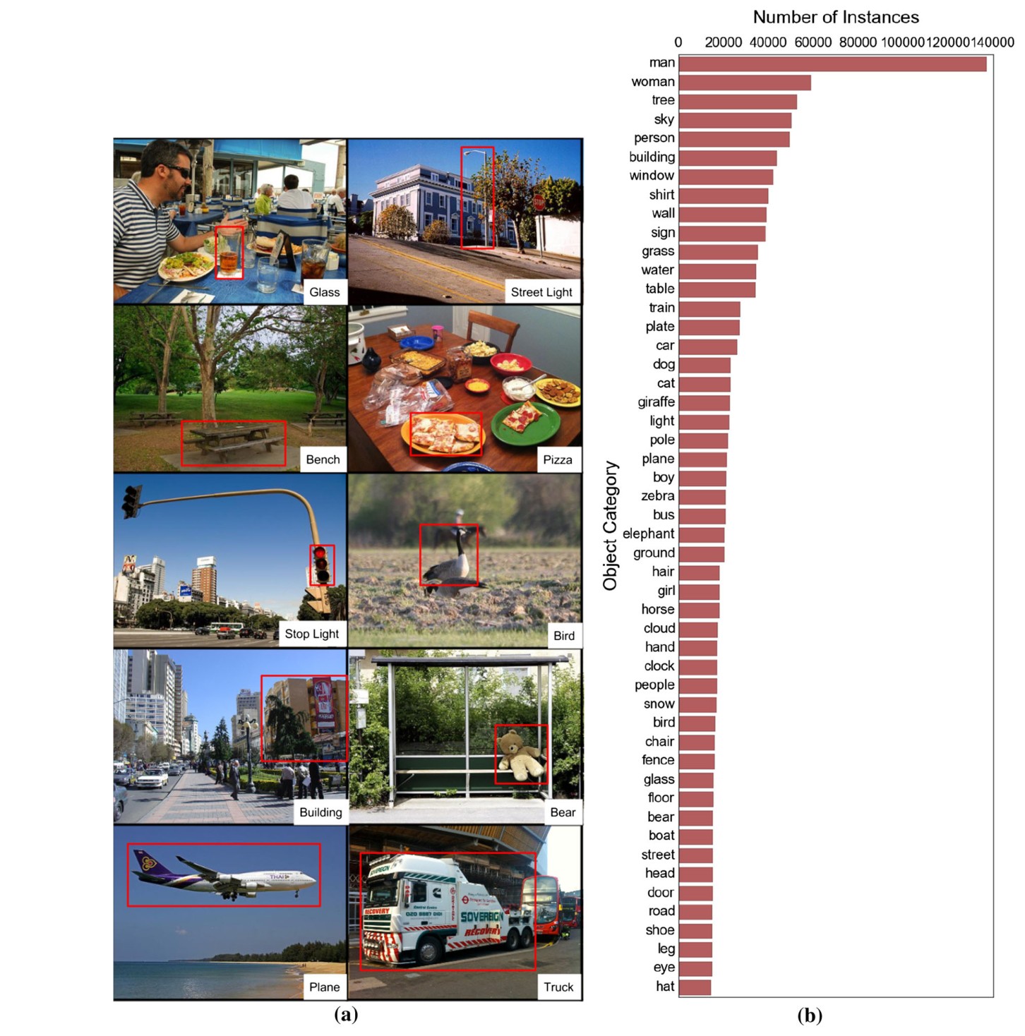
Fig. 22 a Examples of objects in Visual Genome. Each object is localized in its image with a tightly drawn bounding box. b Plot of the most frequently occurring objects in images. People are the most frequently occurring objects in our dataset, followed by common objects and visual elements like building, shirt, and sky
图 22 a Visual Genome 中的物体示例。每个物体都在其图像中用紧致边界框定位。b 图像中最常出现的物体。人是我们数据集中出现最频繁的物体,其次是 building、shirt 和 sky 这类常见物体和视觉元素。
5.4 Attribute Statistics
5.4 属性统计
Attributes allow for detailed description and disambiguation of objects in our dataset. Our dataset contains million total attributes with unique attributes. Attributes include colors (e.g. green), sizes (e.g. tall), continuous action verbs (e.g. standing), materials (e.g. plastic), etc. Each object can have multiple attributes.
属性使我们能够对数据集中的物体做细致描写和消歧。我们的数据集共有 万个属性,其中独特属性 个。属性包括颜色(如 green)、大小(如 tall)、持续性动作动词(如 standing)、材料(如 plastic)等。每个物体可以有多个属性。
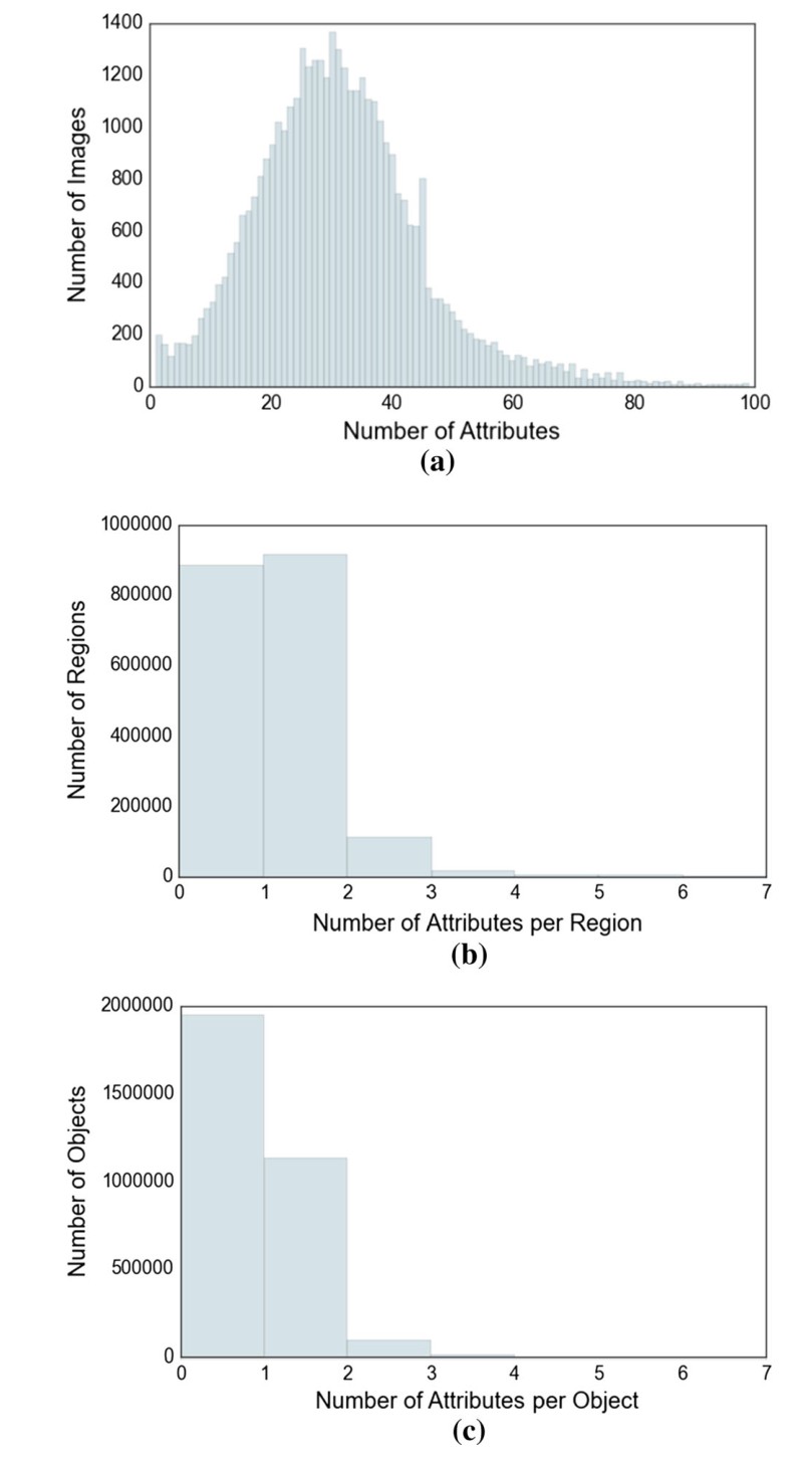
Fig. 23 Distribution of the number of attributes a per image, b per region description, c per object
图 23 属性数量的分布:a 每张图,b 每条区域描述,c 每个物体
On average, each image in Visual Genome contains attributes (Fig. 23). Each region contains on average 1 attribute, though about of regions contain no attribute at all; this is primarily because many regions are relationship-focused. Figure 24a shows the distribution of the most common attributes in our dataset. Colors (e.g. white, green) are by far the most frequent attributes. Also common are sizes (e.g. large) and materials (e.g. wooden). Figure 24b shows the distribution of attributes describing people (e.g. man, girls, and person). The most common attributes describing people are intransitive verbs describing their states of motion (e.g. standing and walking). Certain sports (e.g. skiing, surfboarding) are overrepresented due to an image bias towards these sports.
平均而言,Visual Genome 中的每张图包含 个属性(图 23)。每个区域平均有 1 个属性,不过约 的区域完全没有属性;这主要是因为许多区域是以关系为中心的。图 24a 给出了我们数据集中最常见属性的分布。颜色(如 white、green)显然是最频繁的属性。大小(如 large)和材料(如 wooden)也很常见。图 24b 给出了描述人(如 man、girls 和 person)的属性分布。描述人的最常见属性,是描写其运动状态的不及物动词(如 standing 和 walking)。由于图像偏向这些运动,某些运动(如 skiing、surfboarding)被过度代表。
Attribute Graphs We also qualitatively analyze the attributes in our dataset by constructing co-occurrence graphs, in which nodes are unique attributes and edges connect those attributes that describe the same object. For example, if an image contained a “large black dog” (large(dog), black(dog)) and another image contained a “large yellow cat” (large(cat), yellow(cat)), its attributes would form an incomplete graph with edges (large, black) and (large, yellow). We create two such graphs: one for both the total set of attributes and a second where we consider only objects that refer to people. A subgraph of the 16 most frequently connected (co-occurring) person-related attributes is shown in Fig. 25a.
属性图 我们还通过构建共现图,对数据集中的属性做定性分析:节点是独特属性,边连接那些描述同一物体的属性。例如,如果一幅图中有一只“large black dog”(large(dog)、black(dog)),另一幅图中有一只“large yellow cat”(large(cat)、yellow(cat)),其属性就会形成一个不完整的图,边上是(large,black)和(large,yellow)。我们创建了两张这样的图:一张针对全部属性集合,另一张只考虑指人的物体。图 25a 给出了共现(连接)最频繁的 16 个人物相关属性的一个子图。
Cliques in these graphs represent groups of attributes in which at least one co-occurrence exists for each pair of attributes. In the previous example, if a third image contained a “black and yellow taxi” (black(taxi), yellow(taxi)), the resulting third edge would create a clique between the attributes black, large, and yellow. When calculated across the entire Visual Genome dataset, these cliques provide insight into commonly perceived traits of different types of objects. Figure 25b is a selected representation of three example cliques and their overlaps. From just a clique of attributes, we can predict what types of objects are usually referenced. In Fig. 25b, we see that these cliques describe an animal (left), water body (top right), and human hair (bottom right).
这些图中的团表示这样一组属性:其中每一对属性至少存在一次共现。在前面的例子里,如果第三幅图中有一辆“black and yellow taxi”(black(taxi)、yellow(taxi)),由此产生的第三条边就会在属性 black、large 和 yellow 之间形成一个团。当在整个 Visual Genome 数据集上计算时,这些团有助于洞察不同类型物体通常被感知到的特征。图 25b 是三个示例团及其重叠的一个有选择的展示。仅仅从属性团出发,我们就能推测通常被指称的是哪类物体。在图 25b 中,可以看到这些团分别在描述一种动物(左)、水体(右上)和人类头发(右下)。
Other cliques (not shown) can also uniquely identify object categories. In our set, one clique contains athletic, young, fit, skateboarding, focused, teenager, male, skinny, and happy, capturing some of the common traits of skateboarders in our set. Another such clique has shiny, small, metal, silver, rusty, parked, and empty, most likely describing a subset of cars. From these cliques, we can thus infer distinct objects and object types based solely on their attributes, potentially allowing for highly specific object identification based on selected characteristics.
其他团(未画出)也能唯一标识物体类别。在我们的集合中,一个团包含 athletic、young、fit、skateboarding、focused、teenager、male、skinny 和 happy,抓住了我们集合中 skateboarders 的一些常见特征。另一个这样的团有 shiny、small、metal、silver、rusty、parked 和 empty,最可能是在描述汽车的一个子集。因此,我们可以仅根据属性推断出不同的物体和物体类型,从而有可能基于所选特征做高度具体的物体识别。
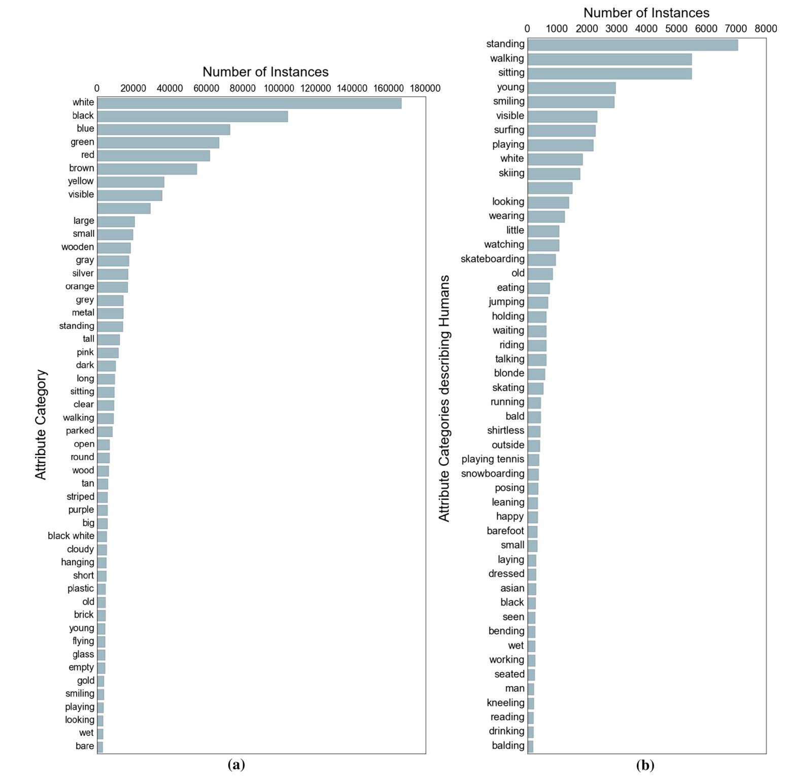
Fig. 24 a Distribution showing the most common attributes in the dataset. Colors (e.g. white, red) and materials (e.g. wooden, metal) are the most common. b Distribution showing the number of attributes describing people. State-of-motion verbs (e.g. standing, walking) are the most common, while certain sports (e.g. skiing, surfing) are also highly represented due to an image source bias in our image set
图 24 a 数据集中最常见属性的分布。颜色(如 white、red)和材料(如 wooden、metal)最为常见。b 描述人的属性数量分布。运动状态动词(如 standing、walking)最常见,某些运动(如 skiing、surfing)也占很高比例,这是因为我们的图像集合在来源上存在偏差。
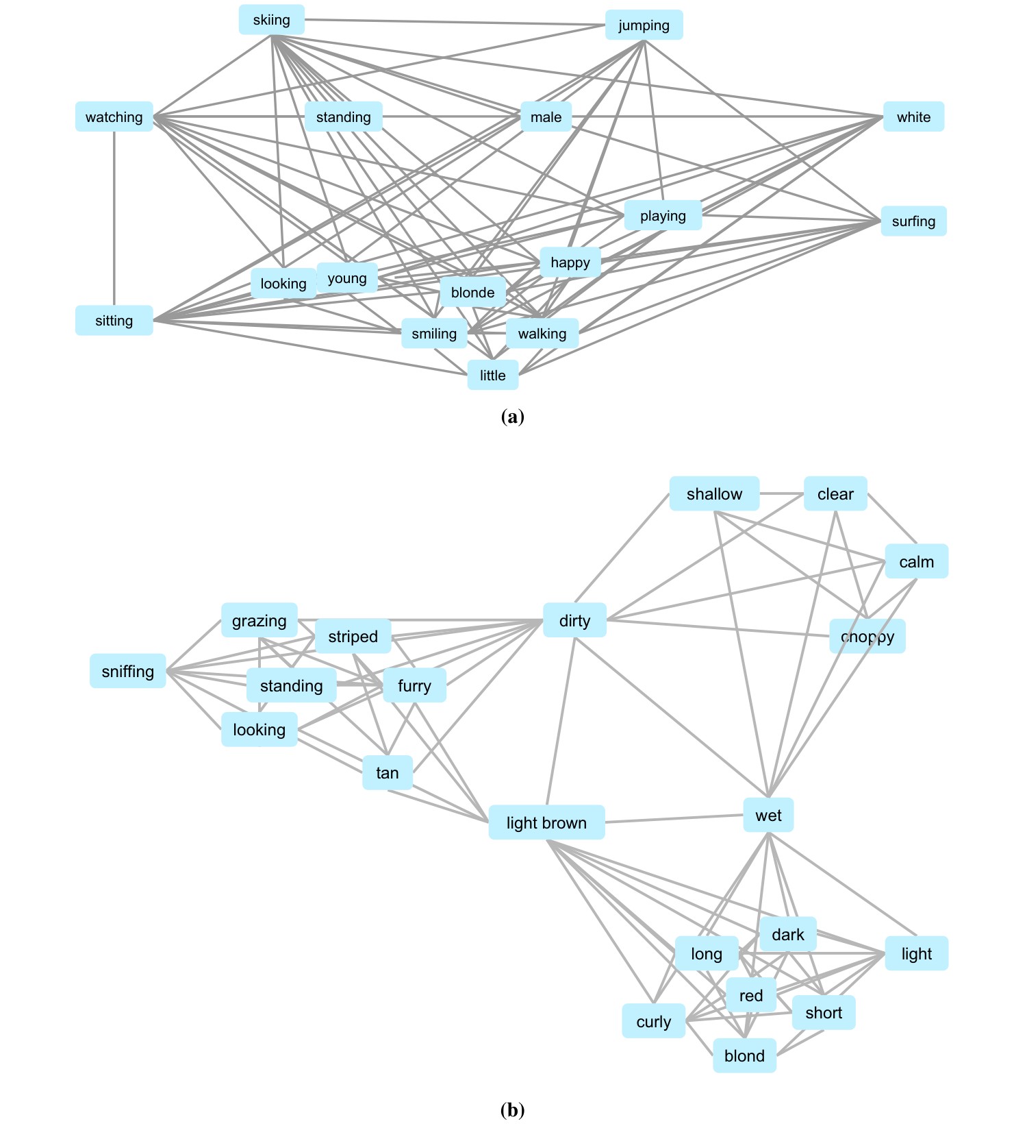
Fig. 25 a Graph of the person-describing attributes with the most co-occurrences. Edge thickness represents the frequency of co-occurrence of the two nodes. b A subgraph showing the co-occurrences and intersections of three cliques, which appear to describe water (top right), hair (bottom right), and some type of animal (left). Edges between cliques have been removed for clarity
图 25 a 共现最多的、用来描述人的属性图。边的粗细表示两个节点共现的频率。b 一个子图,展示三个团的共现与交叉,它们分别像是在描述水(右上)、头发(右下)和某类动物(左)。团与团之间的边已去掉,以便看清结构。
5.5 Relationship Statistics
5.5 关系统计
Relationships are the core components that link objects in our scene graphs. Relationships are directional, i.e. they involve two objects, one acting as the subject and one as the object of a predicate relationship. We denote all relationships in the form relationship(subject, object). For example, if a man is swinging a bat, we write swinging(man, bat). Relationships can be spatial (e.g. inside_of), action (e.g. swinging), compositional (e.g. part_of), etc. More complex relationships such as standing_on, which includes both an action and a spatial aspect, are also represented. Relationships are extracted from region descriptions by crowd workers, similarly to attributes and objects. Visual Genome contains a total of unique relationships, with over million total relationships.
关系是把我们场景图中的物体连接起来的核心组成部分。关系是有方向的,也就是说,它们涉及两个物体,一个作为主语,一个作为谓词关系的宾语。我们把所有关系写成 relationship(subject, object) 的形式。例如,如果一个 man 正在 swinging 一根 bat,我们就写成 swinging(man, bat)。关系可以是空间关系(如 inside_of)、动作(如 swinging)、组成关系(如 part_of)等。像 standing_on 这类同时包含动作和空间方面的更复杂关系也被表示出来。关系由众包工人从区域描述中抽出,方式与属性和物体类似。Visual Genome 共有 种独特关系,关系实例总数超过 个。
Figure 26a shows the distribution of relationships per region description. On average, we have 1 relationship per region, with a maximum of 7. We also have some descriptions like “an old, tall man,” which have multiple attributes associated with the man but no relationships. Figure 26b is a distribution of relationships per image object. Finally, Fig. 26c shows the distribution of relationships per image. Each image has an average of 19 relationships, with a minimum of 1 relationship and with a maximum of over 80 relationships.
图 26a 给出每个区域描述中的关系分布。我们平均每个区域有 1 个关系,最多为 7 个。我们也有一些像“an old, tall man”这样的描述,其中有多个属性与这个 man 相关联,但没有关系。图 26b 是每个图像物体上的关系分布。最后,图 26c 给出每张图上的关系分布。每张图平均有 19 个关系,最少 1 个,最多超过 80 个。
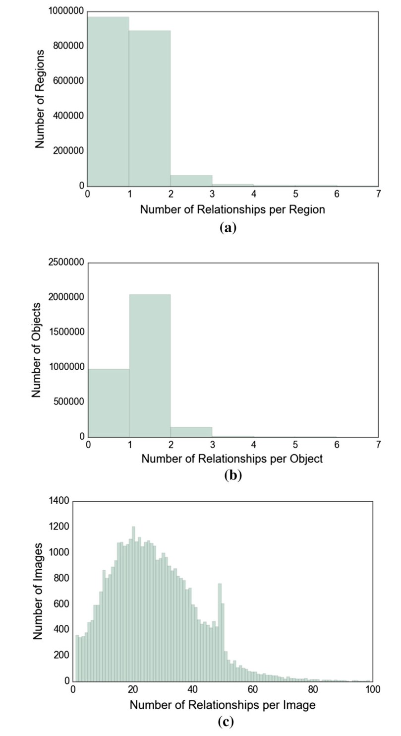
Fig. 26 Distribution of relationships a per image region, b per image object, c per image
图 26 关系数量的分布:a 每个图像区域,b 每个图像物体,c 每张图
Top Relationship Distributions We display the most frequently occurring relationships in Fig. 27a. on is the most common relationship in our dataset. This is primarily because of the flexibility of the word on, which can refer to spatial configuration (on top of), attachment (hanging on), etc. Other common relationships involve actions like holding and wearing and spatial configurations like behind, next to, and under. Figure 27b shows a similar distribution but for relationships involving people. Here we notice more human-centric relationships or actions such as kissing, chatting with, and talking to. The two distributions follow a Zipf distribution.
排名靠前的关系分布 我们在图 27a 中展示出现最频繁的关系。on 是我们数据集中最常见的关系。这主要是因为 on 这个词很灵活,既可以指空间配置(on top of),也可以指附着(hanging on)等。其他常见关系包括 holding 和 wearing 这类动作,以及 behind、next to 和 under 这类空间配置。图 27b 给出类似的分布,但只针对涉及人的关系。在这里我们看到更多以人为中心的关系或动作,如 kissing、chatting with 和 talking to。这两种分布都服从齐普夫分布。
Understanding Affordances Relationships allow us to also understand the affordances of objects. Figure 28a shows the distribution for subjects while Fig. 28b shows a similar distribution for objects. Comparing the two, we find clear patterns of people-like subject entities such as person, man, policeman, boy, and skateboarder that can ride other objects; the other distribution contains objects that afford riding, such as horse, bike, elephant, motorcycle, and skateboard. We can also learn specific common-sense knowledge, like that zebras eat hay and grass while a person eats pizzas and burgers and that couches usually have pillows on them.
理解可供性 关系也让我们能够理解物体的可供性。图 28a 给出主语的分布,图 28b 则给出宾语的类似分布。比较两者,我们可以清楚地看到能够骑乘其他物体的、类似人的主语实体,如 person、man、policeman、boy 和 skateboarder;另一边的分布则包含能够提供 riding 这种可能性的物体,如 horse、bike、elephant、motorcycle 和 skateboard。我们还可以学到具体的常识,例如 zebras 吃 hay 和 grass,而 person 吃 pizzas 和 burgers,以及 couches 上面通常有 pillows。
Related Work Comparison It is also worth mentioning in this section some prior work on relationships. The concept of visual relationships has already been explored in Visual Phrases (Sadeghi and Farhadi 2011), who introduced a dataset of 17 such relationships such as next_to(person, bike) and riding(person, horse). However, their dataset is limited to just these 17 relationships. Similarly, the MS-COCO-a a scene graph dataset (Ronchi and Perona 2015) introduced 156 actions that humans performed in MS-COCO’s dataset (Lin et al. 2014). They show that to exhaustively describe “common” images involving humans, only a small set of visual actions is needed. However, their dataset is limited to just actions, while our relationships are more general and numerous, with over unique relationships. Finally, VisKE (Sadeghi et al. 2015) introduced 6500 relationships, but in a much smaller dataset of images than Visual Genome.
与相关工作的比较 在这一节里也值得提到一些关于关系的先前工作。视觉关系这一概念已经在 Visual Phrases(Sadeghi and Farhadi 2011)中被探讨过,他们推出了一个包含 17 种这类关系的数据集,例如 next_to(person, bike) 和 riding(person, horse)。不过,他们的数据集仅限于这 17 种关系。类似地,MS-COCO-a 这一场景图数据集(Ronchi and Perona 2015)引入了人们在 MS-COCO 数据集(Lin et al. 2014)中执行的 156 种动作。他们表明,要穷尽地描述涉及人的“常见”图像,只需要一小套视觉动作。不过,他们的数据集仅限于动作,而我们的关系更一般、数量也更多,有超过 种独特关系。最后,VisKE(Sadeghi et al. 2015)引入了 6500 种关系,但其图像数据集比 Visual Genome 小得多。
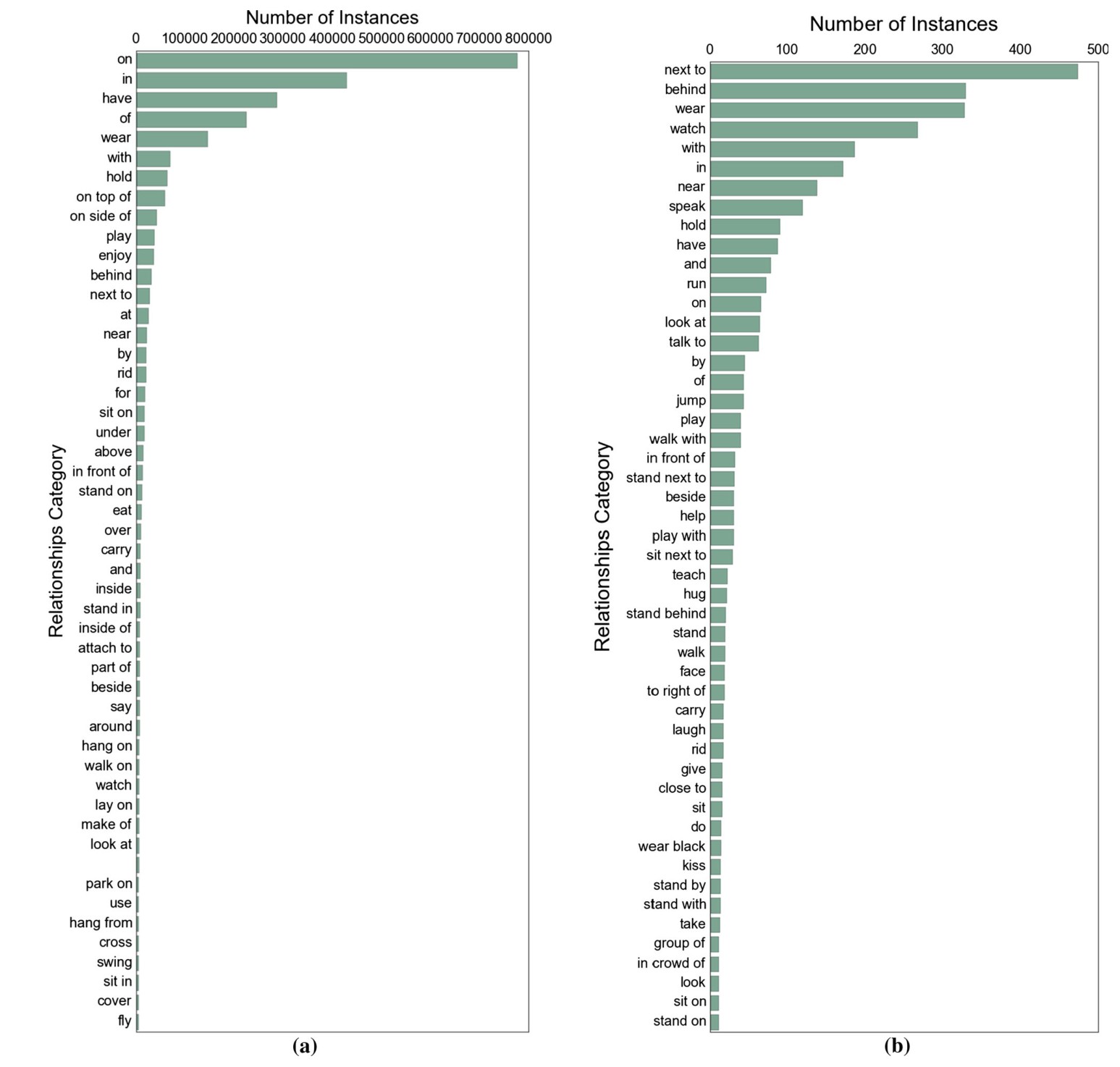
Fig. 27 a A sample of the most frequent relationships in our dataset. In general, the most common relationships are spatial (on top of, on side of, etc.). b A sample of the most frequent relationships involving humans in our dataset. The relationships involving people tend to be more action oriented (walk, speak, run, etc.)
图 27 a 我们数据集中最频繁关系的一个样本。总体而言,最常见的关系是空间关系(on top of、on side of 等)。b 数据集中涉及人的最频繁关系样本。涉及人的关系往往更偏向动作(walk、speak、run 等)。
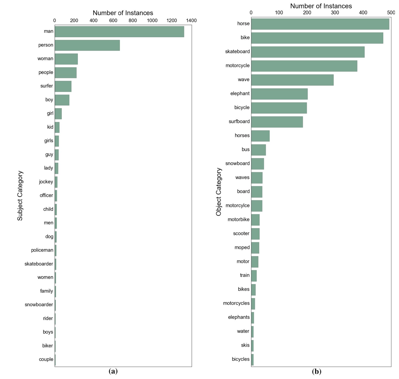
Fig. 28 a Distribution of subjects for the relationship riding. b Distribution of objects for the relationship riding. Subjects comprise of people-like entities like person, man, policeman, boy, and skateboarder that can ride other objects. On the other hand, objects like horse, bike, elephant and motorcycle are entities that can afford riding
图 28 a 关系 riding 的主语分布。b 关系 riding 的宾语分布。主语由 person、man、policeman、boy 和 skateboarder 这类可以骑乘其他物体的、类似人的实体组成。另一方面,horse、bike、elephant 和 motorcycle 这类物体则是能够提供 riding 这种可能性的实体。
5.6 Region and Scene Graph Statistics
5.6 区域图与场景图统计
We introduce in this paper the largest dataset of scene graphs to date. We use these graph representations of images as a deeper understanding of the visual world. In this section, we analyze the properties of these representations, both at the region-level through region graphs and at the image level through scene graphs. We also briefly explore other datasets with scene graphs and provide aggregate statistics on our entire dataset.
本文推出迄今规模最大的场景图数据集。我们把这些图像的图表示,当作对视觉世界更深入的理解来使用。在本节中,我们分析这些表示的性质,既包括通过区域图得到的区域级性质,也包括通过场景图得到的图像级性质。我们也简要考察其他带有场景图的数据集,并给出我们整个数据集的汇总统计。
In previous work, scene graphs have been collected by asking humans to write a list of triples about an image (Johnson et al. 2015). However, unlike them, we collect graphs at a much more fine-grained level: the region graph. We obtained our graphs by asking workers to create them from the descriptions we collected from our regions. Therefore, we end up with multiple graphs for an image, one for every region description. Together, we can combine all the individual region graphs to aggregate a scene graph for an image. This scene graph is made up of all the individual region graphs. In our scene graph representation, we merge all the objects that referenced by multiple region graphs into one node in the scene graph.
在先前工作中,场景图是通过请人就一幅图写下一组三元组来收集的(Johnson et al. 2015)。但与他们不同,我们在更细的粒度上收集图:即区域图。我们的图是请工人根据我们从区域中收集到的描述来创建的。因此,一幅图最终会有多张图,每条区域描述对应一张。我们可以把全部单个区域图合并起来,为整张图汇总出一张场景图。这张场景图由全部单个区域图组成。在我们的场景图表示中,我们把被多个区域图引用的全部物体合并成场景图中的一个节点。
Each of our images has between 5 to 100 region graphs per image, with an average of . Each image has exactly one scene graph. Note that the number of region descriptions and the number of region graphs for an image are not the same. For example, consider the description “it is a sunny day”. Such a description contains no objects, which are the building blocks of a region graph. Therefore, such descriptions have no region graphs associated with them.
我们的每张图有 5 到 100 张区域图,平均为 张。每张图恰好有一张场景图。需要注意,一张图的区域描述数和区域图数并不相同。例如,考虑描述“it is a sunny day”。这样的描述不含物体,而物体是区域图的基本构件。因此,这类描述没有与之对应的区域图。
Objects, attributes, and relationships occur as a normal distribution in our data. Table 4 shows that in a region graph, there are an average of objects, attributes, and relationships. Each scene graph and consequently each image has average of objects, attributes, and relationships.
物体、属性和关系在我们的数据中呈正态分布。表 4 显示,在一张区域图中,平均有 个物体、 个属性和 个关系。每张场景图,因而也就是每张图像,平均有 个物体、 个属性和 个关系。
5.7 Question Answering Statistics
5.7 问答统计
We collected question answering (QA) pairs on the Visual Genome images. Each pair consists of a question and its correct answer regarding the content of an image. On average, every image has QA pairs. Rather than collecting unconstrained QA pairs as previous work has done (Antol et al. 2015; Gao et al. 2015; Malinowski and Fritz 2014), each question in Visual Genome starts with one of the six Ws – what, where, when, who, why, and how. There are two major benefits to focusing on six types of questions. First, they offer a considerable coverage of question types, ranging from basic perceptual tasks (e.g. recognizing objects and scenes) to complex common sense reasoning (e.g. inferring motivations of people and causality of events). Second, these categories present a natural and consistent stratification of task difficulty, indicated by the baseline performance in Sect. 6.4. For instance, why questions that involve complex reasoning lead to the poorest performance ( top-100 accuracy compared to top-100 accuracy of the next lowest) of the six categories. This enables us to obtain a better understanding of the strengths and weaknesses of today’s computer vision models, which sheds light on future directions in which to proceed.
我们在 Visual Genome 的图像上收集了 对问答(QA)。每一对由一个问题及其关于图像内容的正确答案组成。平均每张图有 对问答。与先前工作收集不受约束的问答对不同(Antol et al. 2015; Gao et al. 2015; Malinowski and Fritz 2014),Visual Genome 中的每个问题都以六个 W 之一开头:what、where、when、who、why 和 how。聚焦这六类问题有两大好处。第一,它们对问题类型有相当可观的覆盖,从基本感知任务(例如识别物体和场景)到复杂的常识推理(例如推断人的动机和事件的因果)。第二,这些类别呈现出任务难度上一种自然而一致的分层,这一点由第 6.4 节中的基线表现可以看出。例如,涉及复杂推理的 why 问题,在六类中表现最差(top-100 准确率为 ,而次低的一类是 的 top-100 准确率)。这使我们能够更好地理解当今计算机视觉模型的长处和短处,从而为未来方向提供线索。
Table 4 The average number of objects, attributes, and relationships per region graph and per scene graph
| Objects | Attributes | Relationships | |
|---|---|---|---|
| Region graph | 0.71 | 0.52 | 0.43 |
| Scene graph | 35 | 26 | 21 |
表 4 每个区域图和每张场景图上物体、属性和关系的平均数
| 物体 | 属性 | 关系 | |
|---|---|---|---|
| 区域图 | 0.71 | 0.52 | 0.43 |
| 场景图 | 35 | 26 | 21 |
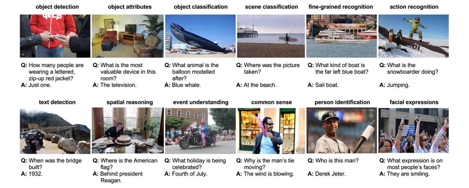
Fig. 29 Example QA pairs in the Visual Genome dataset. Our QA pairs cover a spectrum of visual tasks from recognition to high-level reasoning
图 29 Visual Genome 数据集中的示例问答对。我们的问答对覆盖从识别到高层推理的一系列视觉任务。
We now analyze the diversity and quality of our questions and answers. Our goal is to construct a large-scale visual question answering dataset that covers a diverse range of question types, from basic cognition tasks to complex reasoning tasks. We demonstrate the richness and diversity of our QA pairs by examining the distributions of questions and answers in Fig. 29.
我们现在分析问题和答案的多样性与质量。我们的目标是构建一个大规模视觉问答数据集,覆盖从基本认知任务到复杂推理任务的多样问题类型。我们通过考察图 29 中的问题和答案分布,来展示我们问答对的丰富性与多样性。
Question Type Distributions The questions naturally fall into the 6W categories via their interrogative words. Inside each of the categories, the second and following words categorize the questions with increasing granularity. Inspired by VQA (Antol et al. 2015), we show the distributions of the questions by their first three words in Fig. 30. We can see that “what” is the most common of the six categories. A notable difference between our question distribution and VQA’s is that we focus on ensuring that all six question categories are adequately represented, while in VQA, of the questions are yes/no binary questions. As a result, a trivial model can achieve a reasonable performance by just predicting “yes” or “no” as answers. We encourage more difficult QA pairs by ruling out binary questions.
问题类型分布 这些问题按其疑问词自然落入 6W 类别。在每个类别内部,第二个及随后的词又以更细的粒度给问题分类。受 VQA(Antol et al. 2015)启发,我们在图 30 中按前三个词给出问题分布。可以看到,“what”是六类中最常见的。我们的问题分布与 VQA 的一个显著差别在于,我们着重确保全部六类问题都得到充分代表,而在 VQA 中, 的问题是是非二值问题。其结果是,一个平凡模型只需预测“yes”或“no”作为答案,就能取得还过得去的表现。我们通过排除二值问题,来鼓励更难的问答对。
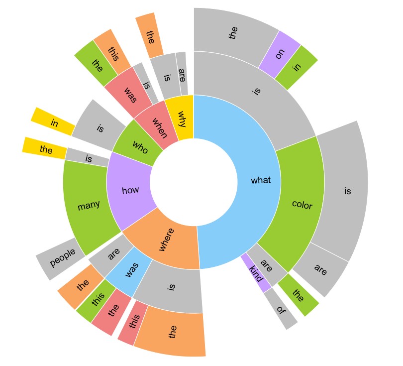
Fig. 30 Distribution of question types by starting words. This figure shows the distribution of the questions by their first three words. The angles of the regions are proportional to the number of pairs from the corresponding categories. We can see that “what” questions are the largest category with nearly half of the QA pairs
图 30 按起始词划分的问题类型分布。本图按问题的前三个词给出分布。各区域的角度与对应类别中的问答对数成正比。可以看到,“what”类问题是最大的一类,接近问答对的一半。
Question and Answer Length Distributions We also analyze the question and answer lengths of each 6W category. Figure 31 shows the average question and answer lengths of each category. Overall, the average question and answer lengths are 5.7 and 1.8 words respectively. In contrast to the VQA dataset, where , , and of the answers consist of one, two, or three words, our answers exhibit a long-tail distribution where , , and of the answers have one, two, or three words respectively. We avoid verbosity by instructing the workers to write answers as concisely as possible. The coverage of long answers means that many answers contain a short description that contains more details than merely an object or an attribute. It shows the richness and complexity of our visual QA tasks beyond object-centric recognition tasks. We foresee that these long-tail answers can motivate future research in common-sense reasoning and high-level image understanding.
问句和答句长度分布 我们也分析了每个 6W 类别的问句和答句长度。图 31 给出了各类的平均问句长度和答句长度。总体而言,平均问句长度为 5.7 个词,平均答句长度为 1.8 个词。与 VQA 数据集中 、 和 的答案分别由一个、两个或三个词组成形成对照,我们的答案呈长尾分布,其中 、 和 的答案分别有一个、两个或三个词。我们通过要求工人尽量把答案写得简洁,来避免冗长。长答案的覆盖意味着,许多答案包含一段短描述,其中的细节比单单一个物体或一个属性更多。这显示出,我们的视觉问答任务在以物体为中心的识别任务之外,还具有丰富性和复杂性。我们预期,这些长尾答案可以推动未来在常识推理和高层图像理解方面的研究。
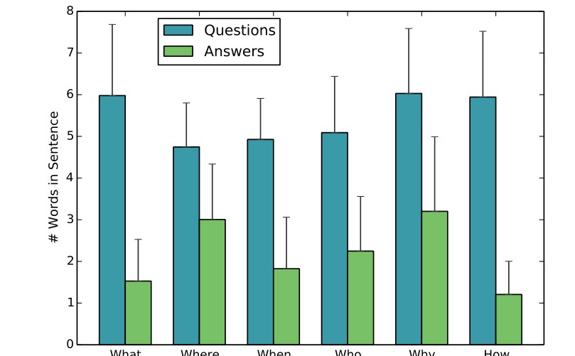
Fig. 31 Question and answer lengths by question type. The bars show the average question and answer lengths of each question type. The whiskers show the standard deviations. The factual questions, such as “what” and “how” questions, usually come with short answers of a single object or a number. This is only because “how” questions are disproportionately counting questions that start with “how many”. Questions from the “where” and “why” categories usually have phrases and sentences as answers
图 31 各类问题的问句和答句长度。柱子表示每类问题的平均问句长度和答句长度。须线表示标准差。像“what”和“how”这类事实性问题,答案通常很短,往往是单个物体或一个数字。这只是因为“how”问题中,以“how many”开头的计数问题占了不成比例的份额。“where”和“why”类问题的答案通常是短语和句子。
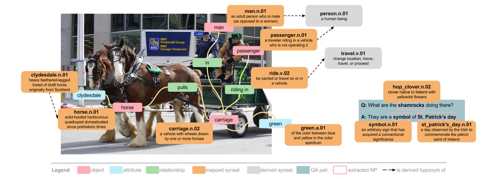
Fig. 32 An example image from the Visual Genome dataset with its region descriptions, QA pairs, objects, attributes, and relationships canonicalized. The large text boxes are WordNet synsets referenced by this image. For example, the carriage is mapped to carriage.n.02: a vehicle with wheels drawn by one or more horses. We do not show the bounding boxes for the objects in order to allow readers to see the image clearly. We also only show a subset of the scene graph for this image to avoid cluttering the figure
图 32 Visual Genome 数据集中的一张示例图像,其区域描述、问答对、物体、属性和关系都已规范化。大文本框是这张图所引用的 WordNet 同义词集。例如,carriage 被映射到 carriage.n.02: a vehicle with wheels drawn by one or more horses. 为了让读者看清图像,我们没有画出物体的边界框。为避免图面过于拥挤,我们也只展示了这张图场景图的一个子集。
5.8 Canonicalization Statistics
5.8 规范化统计
In order to reduce the ambiguity in the concepts of our dataset and connect it to other resources used by the research community, we canonicalize the semantic meanings of all objects, relationships, and attributes in Visual Genome. By “canonicalization,” we refer to word sense disambiguation (WSD) by mapping the components in our dataset to their respective synsets in the WordNet ontology (Miller 1995). This mapping reduces the noise in the concepts contained in the dataset and also facilitates the linkage between Visual Genome and other data sources such as ImageNet (Deng et al. 2009), which is built on top of the WordNet ontology.
为了降低数据集概念中的歧义,并把它与研究社区使用的其他资源连接起来,我们把 Visual Genome 中全部物体、关系和属性的语义加以规范化。这里的“规范化”,指的是通过把数据集中的组成部分映射到 WordNet 本体(Miller 1995)中各自的同义词集,来做词义消歧(WSD)。这种映射降低了数据集所含概念中的噪声,也便于把 Visual Genome 与建立在 WordNet 本体之上的 ImageNet(Deng et al. 2009)等其他数据源连接起来。
Figure 32 shows an example image from the Visual Genome dataset with its components canonicalized. For example, horse is canonicalized as horse.n.01: solid-hoofed herbivorous quadruped domesticated since prehistoric times. Its attribute, clydesdale, is canonicalized as its breed clydesdale.n.01: heavy feathered-legged breed of draft horse originally from Scotland. We also show an example of a QA from which we extract the nouns shamrocks, symbol, and St. Patrick’s day, all of which we canonicalize to WordNet as well.
图 32 给出 Visual Genome 数据集中一张示例图像及其已被规范化的各个部分。例如,horse 被规范化为 horse.n.01: solid-hoofed herbivorous quadruped domesticated since prehistoric times。它的属性 clydesdale 被规范化为其品种 clydesdale.n.01: heavy feathered-legged breed of draft horse originally from Scotland。我们还给出一个问答例子,从中抽出名词 shamrocks、symbol 和 St. Patrick’s day,它们同样都被规范化到 WordNet。
Related Work Canonicalization, or WSD (Pal and Saha 2015), has been used in numerous applications, including machine translation, information retrieval, and information extraction (Rothe and Schütze 2015; Leacock et al. 1998). In English sentences, sentences like “He scored a goal” and “It was his goal in life” carry different meanings for the word “goal.” Understanding these differences is crucial for translating languages and for returning correct results for a query. Similarly, in Visual Genome, we ensure that all our components are canonicalized to understand how different objects are related to each other; for example, “person” is a hypernym of “man” and “woman.” Most past canonicalization models use precision, recall, and F1 score to evaluate on the Semeval dataset (Mihalcea et al. 2004). The current state-of-the-art performance on Semeval is an F1 score of (Chen et al. 2014). Since our canonicalization setup is different from the Semeval benchmark (we have an open vocabulary and no annotated ground truth for evaluation), our canonicalization method is not directly comparable to these existing methods. We do however, achieve a similar precision and recall score on a held-out test set described below (Table 5).
相关工作 规范化,亦即词义消歧(WSD)(Pal and Saha 2015),已用于机器翻译、信息检索和信息抽取等众多应用(Rothe and Schütze 2015; Leacock et al. 1998)。在英语句子中,“He scored a goal”和“It was his goal in life”里的“goal”含义不同。理解这些差别,对于翻译语言和为查询返回正确结果至关重要。类似地,在 Visual Genome 中,我们确保所有组成部分都被规范化,以便理解不同物体如何相互关联;例如,“person”是“man”和“woman”的上位词。过去大多数规范化模型使用精确率、召回率和 F1 分数,在 Semeval 数据集(Mihalcea et al. 2004)上做评估。目前在 Semeval 上的最好成绩是 F1 为 (Chen et al. 2014)。由于我们的规范化设定与 Semeval 基准不同(我们使用开放词表,也没有用于评估的已标注真值),我们的规范化方法不能与这些现有方法直接比较。不过,我们在下文所述的留出测试集上,仍然取得了相近的精确率和召回率(表 5)。
Region Descriptions and QAs We canonicalize all objects mentioned in all region descriptions and QA pairs. Because objects need to be extracted from the phrase text, we use Stanford NLP tools (Manning et al. 2014) to extract the noun phrases in each region description and QA, resulting in recall of noun phrases from a subset of 200 region descriptions we manually annotated. After obtaining the noun phrases, we map each to its most frequent matching synset (according to WordNet lexeme counts). This resulted in an overall mapping accuracy of and a recall of (Fig. 5). The most common synsets extracted from region descriptions, QAs, and objects are shown in Fig. 33.
区域描述和问答 我们把全部区域描述和问答对中提到的全部物体都加以规范化。因为物体需要从短语文本中抽出,我们使用斯坦福自然语言处理工具(Manning et al. 2014)抽出每条区域描述和问答中的名词短语,在我们手工标注的 200 条区域描述子集上,名词短语的召回率为 。得到名词短语后,我们按 WordNet 词位计数,把每一个映射到最频繁匹配的同义词集。这带来了总体 的映射准确率和 的召回率(表 5)。从区域描述、问答和物体中抽出的最常见同义词集见图 33。
Table 5 Precision, recall, and mapping accuracy percentages for object, attribute, and relationship canonicalization
| Precision | Recall | |
|---|---|---|
| Objects | 88.0 | 98.5 |
| Attributes | 85.7 | 95.9 |
| Relationships | 92.9 | 88.5 |
表 5 物体、属性和关系规范化的精确率、召回率和映射准确率(百分比)
| 精确率 | 召回率 | |
|---|---|---|
| 物体 | 88.0 | 98.5 |
| 属性 | 85.7 | 95.9 |
| 关系 | 92.9 | 88.5 |
Attributes We canonicalize attributes from the crowd-extracted attributes present in our scene graphs. The “attribute” designation encompasses a wide range of grammatical parts of speech. Because part-of-speech taggers rely on high-level syntax information and thus fail on the disjoint elements of our scene graphs, we normalize each attribute based on morphology alone (so-called “stemming” (Bird 2006)). Then, as with objects, we map each attribute phrase to the most frequent matching WordNet synset. We include 15 hand-mapped rules to address common failure cases in which WordNet’s frequency counts prefer abstract senses of words over the spatial senses present in visual data, e.g. short.a.01: limited in duration over short.a.02: lacking in length. For verification, we randomly sample 200 attributes, produce ground-truth mappings by hand, and compare them to the results of our algorithm. This resulted in a recall of and a mapping accuracy of . The most common attribute synsets are shown in Fig. 34a.
属性 我们从场景图中由众包抽出的属性出发来做规范化。“属性”这一名称涵盖了很广的语法词类。由于词性标注器依赖高层句法信息,因而会在我们场景图中互不连接的元素上失败,我们只基于形态对每个属性做规范化(所谓“词干提取”(Bird 2006))。然后,与物体一样,我们把每个属性短语映射到最频繁匹配的 WordNet 同义词集。我们加入了 15 条手工映射规则,以处理常见的失败情形:在这些情形中,WordNet 的频率计数更偏向词的抽象义项,而不是视觉数据中出现的空间义项,例如偏向 short.a.01: limited in duration 而不是 short.a.02: lacking in length。为了核验,我们随机抽取 200 个属性,手工给出真值映射,再与我们算法的结果相比较。这带来了 的召回率和 的映射准确率。最常见的属性同义词集见图 34a。
Relationships As with attributes, we canonicalize the relationships isolated in our scene graphs. We exclude prepositions, which are not recognized in WordNet, leaving a set primarily composed of verb relationships. Since the meanings of verbs are highly dependent upon their morphology and syntactic placement (e.g. passive cases, prepositional phrases), we map the structure of each relationship to the appropriate WordNet sentence frame and only consider those WordNet synsets with matching sentence frames. For each verb-synset pair, we then consider the root hypernym of that synset to reduce potential noise from WordNet’s fine-grained sense distinctions. We also include 20 hand-mapped rules, again to correct for WordNet’s lower representation of concrete or spatial senses; for example, the concrete hold.v.02: have or hold in one’s hand or grip is less frequent in WordNet than the abstract hold.v.01: cause to continue in a certain state. For verification, we again randomly sample 200 relationships and compare the results of our canonicalization against ground-truth mappings. This resulted in a recall of and a mapping accuracy of . While several datasets, such as VerbNet (Schuler 2005) and FrameNet (Baker et al. 1998), include semantic restrictions or frames to improve classification, there is no comprehensive method of mapping to those restrictions or frames. The most common relationship synsets are shown in Fig. 34b.
关系 与属性一样,我们对隔离在场景图中的关系加以规范化。我们排除 WordNet 中不被识别的介词,剩下的集合主要以动词关系为主。由于动词的意义高度依赖于其形态和句法位置(例如被动情形、介词短语),我们把每个关系的结构映射到相应的 WordNet 句子框架,并只考虑具有匹配句子框架的那些 WordNet 同义词集。对每一对动词–同义词集,我们再考虑该同义词集的根上位词,以降低 WordNet 细粒度义项区分可能带来的噪声。我们还加入了 20 条手工映射规则,同样是为了纠正 WordNet 对具体或空间义项表征不足的问题;例如,具体的 hold.v.02: have or hold in one’s hand or grip 在 WordNet 中不如抽象的 hold.v.01: cause to continue in a certain state 常见。为了核验,我们再次随机抽取 200 个关系,并把规范化结果与真值映射相比较。这带来了 的召回率和 的映射准确率。虽然 VerbNet(Schuler 2005)和 FrameNet(Baker et al. 1998)等若干数据集包含用来改进分类的语义限制或框架,但并没有把内容映射到这些限制或框架的完备方法。最常见的关系同义词集见图 34b。
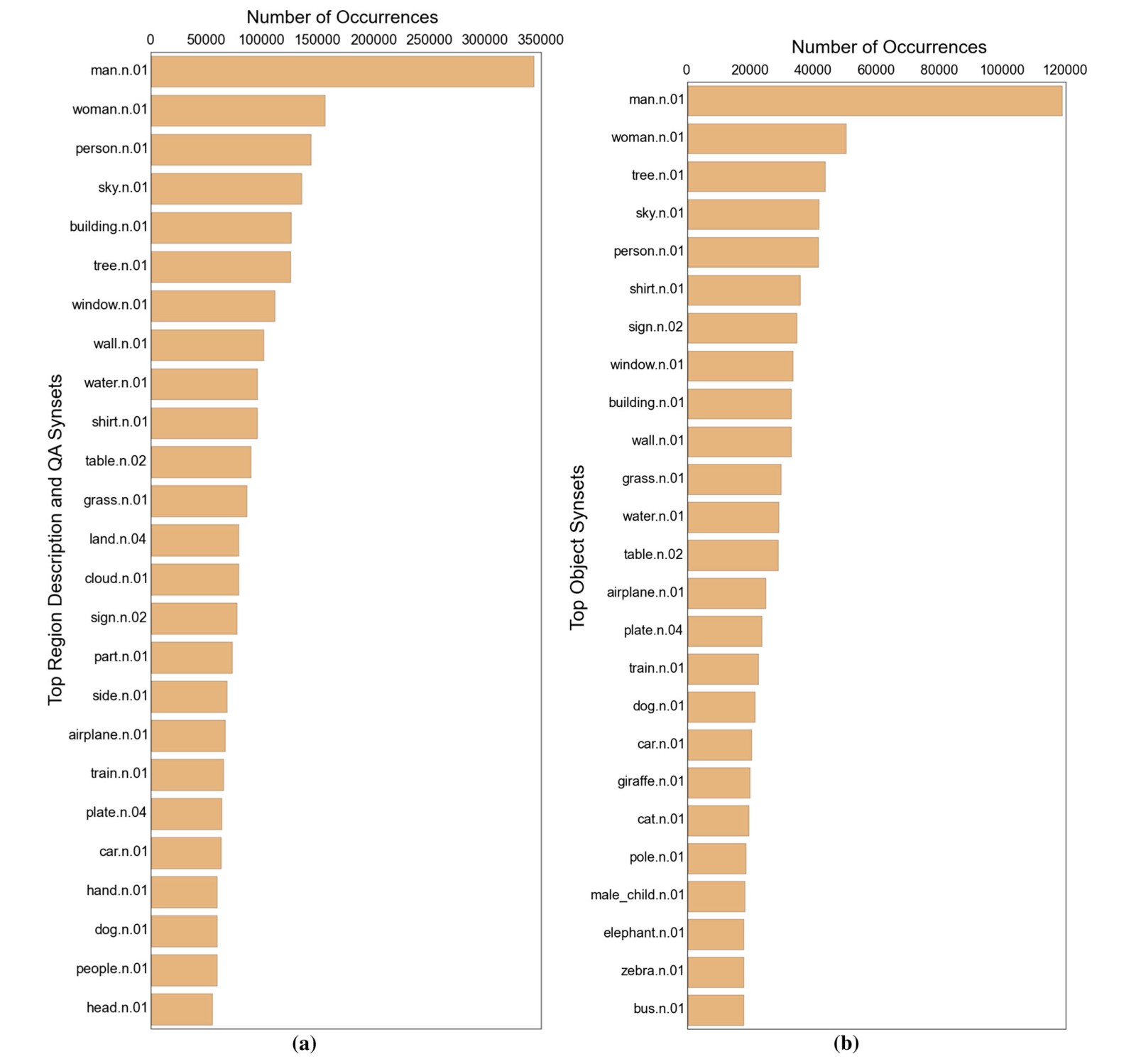
Fig. 33 Distribution of the 25 most common synsets mapped from the words and phrases extracted from region descriptions which represent objects in a region descriptions and question answers and b objects
图 33 从区域描述中抽出的词和短语所映射到的、最常见的 25 个同义词集的分布,这些词和短语表示 a 区域描述和问答中的物体,以及 b 物体本身。
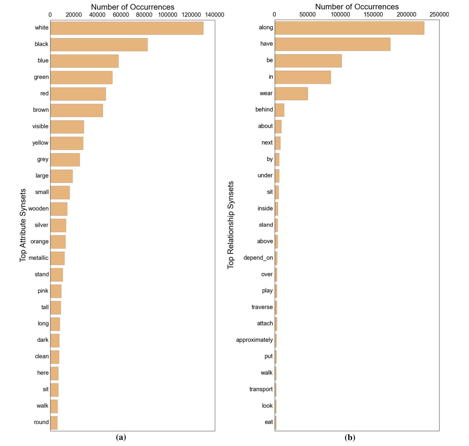
Fig. 34 Distribution of the 25 most common synsets mapped from a attributes and b relationships
图 34 从 a 属性和 b 关系映射得到的、最常见的 25 个同义词集的分布
6 Experiments
6 实验
Thus far, we have presented the Visual Genome dataset and analyzed its individual components. With such rich information provided, numerous perceptual and cognitive tasks can be tackled. In this section, we aim to provide baseline experimental results using components of Visual Genome that have not been extensively studied.
到目前为止,我们已经介绍了 Visual Genome 数据集,并分析了它的各个组成部分。有了这样丰富的信息,许多感知和认知任务都可以着手处理。在本节中,我们的目标是利用 Visual Genome 中尚未被广泛研究的组成部分,给出基准实验结果。
Object detection is already a well-studied problem (Everingham et al. 2010; Girshick et al. 2014; Sermanet et al. 2013; Girshick 2015; Ren et al. 2015b). Similarly, region graphs and scene graphs have been shown to improve semantic image retrieval (Johnson et al. 2015; Schuster et al. 2015). We therefore focus on the remaining components, i.e. attributes, relationships, region descriptions, and question answer pairs.
物体检测已经是一个被充分研究的问题(Everingham et al. 2010; Girshick et al. 2014; Sermanet et al. 2013; Girshick 2015; Ren et al. 2015b)。类似地,区域图和场景图已被证明可以改进语义图像检索(Johnson et al. 2015; Schuster et al. 2015)。因此,我们把重点放在其余组成部分上,即 属性、关系、区域描述 和 问答对。
In Sect. 6.1, we present results for two experiments on attribute prediction. In the first, we treat attributes independently from objects and train a classifier for each attribute, i.e. a classifier for red or a classifier for old, as in Malisiewicz et al. (2008), Varma and Zisserman (2005),Ferrari and Zisserman (2007), Farhadi et al. (2009) and Johnson et al. (2015). In the second experiment, we learn object and attribute classifiers jointly and predict object-attribute pairs (e.g. predicting that an apple is red), as in Sadeghi and Farhadi (2011).
在第 6.1 节,我们给出属性预测上两项实验的结果。第一项中,我们把属性与物体分开处理,并为每个属性训练一个分类器,即一个用于 red 的分类器或一个用于 old 的分类器,一如 Malisiewicz et al.(2008)、Varma and Zisserman(2005)、Ferrari and Zisserman(2007)、Farhadi et al.(2009)以及 Johnson et al.(2015)。在第二项实验中,我们 联合 学习物体和属性分类器,并预测物体–属性对(例如预测一只 apple 是 red),一如 Sadeghi and Farhadi(2011)。
In Sect. 6.2, we present two experiments on relationship prediction. In the first, we aim to predict the predicate between two objects, e.g. predicting the predicate kicking or wearing between two objects. This experiment is synonymous with existing work in action recognition (Gupta et al. 2009; Ramanathan et al. 2015). In another experiment, we study relationships by classifying jointly the objects and the predicate (e.g. predicting kicking(man, ball)); we show that this is a very difficult task due to the high variability in the appearance of a relationship (e.g. the ball might be on the ground or in mid-air above the man). These experiments are generalizations of tasks that study spatial relationships between objects and ones that jointly reason about the interaction of humans with objects (Yao and Fei-Fei 2010; Prest et al. 2012).
在第 6.2 节,我们给出关系预测上的两项实验。第一项中,我们的目标是预测两个物体之间的谓词,例如预测两个物体之间的谓词 kicking 或 wearing。这项实验与动作识别中的现有工作同义(Gupta et al. 2009; Ramanathan et al. 2015)。在另一项实验中,我们通过联合分类物体和谓词来研究关系(例如预测 kicking(man, ball));我们表明,由于一种关系在外观上的高度可变性,这是一项非常困难的任务(例如,ball 可能在地上,也可能悬在 man 上方的空中)。这些实验是对研究物体之间空间关系、以及联合推理人与物体互动的那些任务的推广(Yao and Fei-Fei 2010; Prest et al. 2012)。
In Sect. 6.3 we present results for region captioning. This task is closely related to image captioning (Chen et al. 2015); however, results from the two are not directly comparable, as region descriptions are short, incomplete sentences. We train one of the top 16 state-of-the-art image caption generators (Karpathy and Fei-Fei 2015) on (1) our dataset to generate region descriptions and on (2) Flickr30K (Young et al. 2014) to generate sentence descriptions. To compare results between the two training approaches, we use simple templates to convert region descriptions into complete sentences. For a more robust evaluation, we validate the descriptions we generate using human judgment.
在第 6.3 节,我们给出区域配文的结果。这项任务与图像配文密切相关(Chen et al. 2015);不过,两者的结果不能直接比较,因为区域描述是简短、不完整的句子。我们把 16 个最先进的图像配文生成器之一(Karpathy and Fei-Fei 2015)分别在(1)我们的数据集上训练以生成区域描述,以及在(2)Flickr30K(Young et al. 2014)上训练以生成句子描述。为了比较这两种训练方式的结果,我们使用简单模板把区域描述转换成完整句子。为了做更稳健的评估,我们用人工判断来核验所生成的描述。
Finally, in Sect. 6.4, we experiment on visual question answering, i.e. given an image and a question, we attempt to provide an answer for the question. We report results on the retrieval of the correct answer from a list of existing answers.
最后,在第 6.4 节,我们在视觉问答上做实验,即给定一幅图和一个问题,我们试图为该问题给出答案。我们报告的结果,是从已有答案列表中检索出正确答案。
6.1 Attribute Prediction
6.1 属性预测
Attributes are becoming increasingly important in the field of computer vision, as they offer higher-level semantic cues for various problems and lead to a deeper understanding of images. We can express a wide variety of properties through attributes, such as form (sliced), function (decorative), sentiment (angry), and even intention (helping). Distinguishing between similar objects (Isola et al. 2015) leads to finer-grained classification, while describing a previously unseen class through attributes shared with known classes can enable “zero-shot” learning (Farhadi et al. 2009; Lampert et al. 2009). Visual Genome is the largest dataset of attributes, with attributes per image for more than million attributes.
属性在计算机视觉领域正变得越来越重要,因为它们为各类问题提供更高层的语义线索,并带来对图像更深入的理解。我们可以通过属性表达各种各样的性质,例如形态(sliced)、功能(decorative)、情绪(angry),甚至意图(helping)。区分相似物体(Isola et al. 2015)会导向更细粒度的分类,而通过与已知类别共享的属性来描述一个先前未见过的类别,则可以促成“零样本”学习(Farhadi et al. 2009; Lampert et al. 2009)。Visual Genome 是目前最大的属性数据集,每张图有 个属性,属性总数超过 万。
Setup For both experiments, we focus on the 100 most common attributes in our dataset. We only use objects that occur at least 100 times and are associated with one of the 100 attributes in at least one image. For both experiments, we follow a similar data pre-processing pipeline. First, we lowercase, lemmatize (Bird 2006), and strip excess whitespace from all attributes. Since the number of examples per attribute class varies, we randomly sample 500 attributes from each category (if fewer than 500 are in the class, we take all of them).
实验设置 两项实验都聚焦于数据集中最常见的 100 个属性。我们只用出现至少 100 次、并且至少在一张图中与这 100 个属性之一相关联的物体。两项实验都遵循相似的数据预处理流程。首先,我们对全部属性做小写化、词形还原(Bird 2006),并去掉多余空白。由于每个属性类别的样例数多少不一,我们从每个类别中随机抽取 500 个属性(若该类不足 500 个,则全部取用)。
We end up with around 50, 000 attribute instances and 43, 000 object-attribute pair instances in total. We use of the images for training and each for validation and testing. Because each image has about the same number of examples, this results in an approximately 80–10–10% split over the attributes themselves. The input data for this experiment is the cropped bounding box of the object associated with each attribute.
我们最终大约得到 50,000 个属性实例,以及总计 43,000 个物体–属性对实例。我们把 的图像用于训练,验证和测试各用 。因为每张图的样例数大致相当,这在属性本身上也大致形成了 80–10–10% 的划分。本实验的输入数据,是与每个属性相关联的物体的裁切边界框。
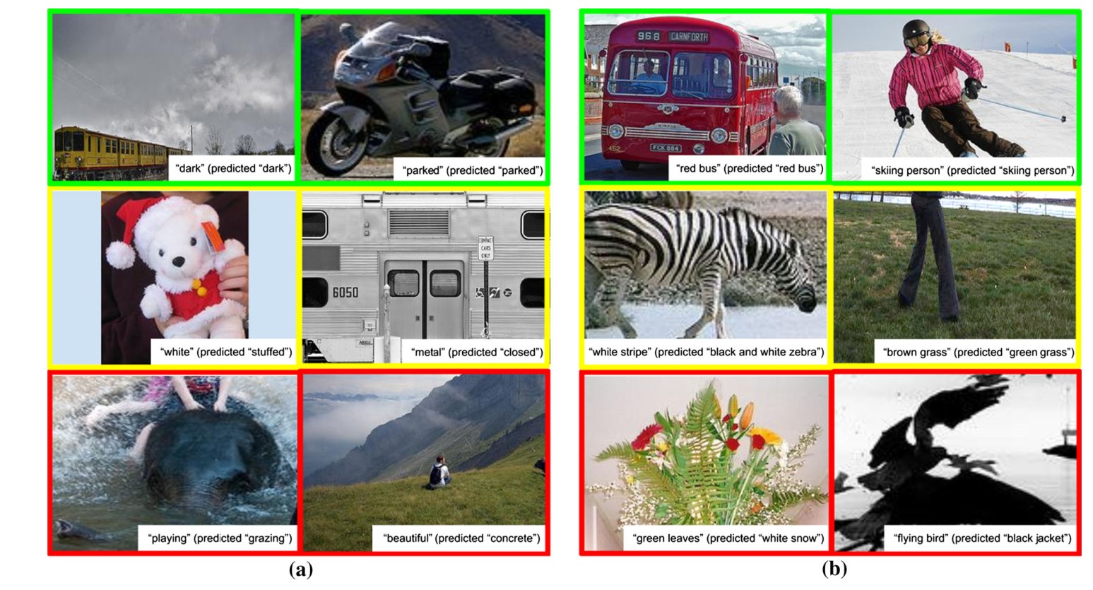
Fig. 35 a Example predictions from the attribute prediction experiment. Attributes in the first row are predicted correctly, those in the second row differ from the ground truth but still correctly classify an attribute in the image, and those in the third row are classified incorrectly. The model tends to associate objects with attributes (e.g. elephant with grazing). b Example predictions from the joint object-attribute prediction experiment
图 35 a 属性预测实验中的示例预测。第一行属性预测正确,第二行与真值不同但仍然正确分类了图中的一个属性,第三行分类错误。模型往往把物体和属性联系起来(例如把 elephant 与 grazing 联系起来)。b 联合物体–属性预测实验中的示例预测。
We train an attribute predictor by using features learned from a convolutional neural network. Specifically, we use a 16-layer VGG network (Simonyan and Zisserman 2014) pre-trained no ImageNet and fine-tune it for both of these experiments using the 50, 000 attribute and 43, 000 object-attribute pair instances respectively. We modify the network so that the learning rate of the final fully-connected layer is 10 times that of the other layers, as this improves convergence time. Convergence is measured as the performance on the validation set. We use a base learning rate of 0.001, which we scale by 0.1 every 200 iterations, and momentum and weight decays of 0.9 and 0.0005 respectively. We use the fine-tuned features from the network and train 100 individual SVMs (Hearst et al. 1998) to predict each attribute. We output multiple attributes for each bounding box input. For the second experiment, we also output the object class.
我们用卷积神经网络学到的特征来训练属性预测器。具体而言,我们使用在 ImageNet 上预训练的 16 层 VGG 网络(Simonyan and Zisserman 2014),并分别用这 50,000 个属性实例和 43,000 个物体–属性对实例,为这两项实验做微调。我们修改网络,使最后一层全连接层的学习率为其他层的 10 倍,因为这能改进收敛时间。收敛以验证集上的表现为度量。我们使用 0.001 的基础学习率,每 200 次迭代将其乘以 0.1,动量和权重衰减分别为 0.9 和 0.0005。我们使用网络微调后的特征,并训练 100 个独立的支持向量机(Hearst et al. 1998)来预测每个属性。我们对每个边界框输入输出多个属性。在第二项实验中,我们也输出物体类别。
Results Table 6 shows results for both experiments. For the first experiment on attribute prediction, we converge after around 700 iterations with top-one accuracy and top-five accuracy. Thus, attributes (like objects) are visually distinguishable from each other. For the second experiment where we also predict the object class, we converge after around 400 iterations with top-one accuracy and top-five accuracy. Predicting objects jointly with attributes increases the top-one accuracy from to . This implies that some attributes occur exclusively with a small number of objects. Additionally, by jointly learning attributes with objects, we increase the inter-class variance, making the classification process an easier task.
结果 表 6 给出两项实验的结果。在第一项属性预测实验中,我们大约在 700 次迭代后收敛,top-1 准确率为 ,top-5 准确率为 。因此,属性(与物体一样)在视觉上是可以相互区分的。在同时预测物体类别的第二项实验中,我们大约在 400 次迭代后收敛,top-1 准确率为 ,top-5 准确率为 。把物体与属性联合预测,把 top-1 准确率从 提高到 。这意味着,有些属性只与少数物体一同出现。此外,通过与物体联合学习属性,我们增大了类间方差,使分类过程成为一项更容易的任务。
Figure 35a shows example predictions for the first attribute prediction experiment. In general, the model is good at associating objects with their most salient attributes, for example, animal with stuffed and elephant with grazing. However, the crowdsourced ground truth answers sometimes do not contain all valid attributes, so the model is incorrectly penalized for some accurate/true predictions. For example, the white stuffed animal is correct but evaluated as incorrect.
图 35a 给出第一项属性预测实验的示例预测。总体而言,模型擅长把物体与其最显著的属性联系起来,例如把 animal 与 stuffed 联系起来,把 elephant 与 grazing 联系起来。不过,众包得到的真值答案有时并不包含全部有效属性,因此模型会因一些准确/正确的预测而受到错误惩罚。例如,白色的毛绒玩具是正确的,却被评为不正确。
Figure 35b shows example predictions for the second experiment in which we also predict the object. While the results in the second row might be considered correct, to keep a consistent evaluation, we mark them as incorrect. For example, the predicted “green grass” might be considered subjectively correct even though it is annotated as “brown grass”. For cases where the objects are not clearly visible but are abstract outlines, our model is unable to predict attributes or objects accurately. For example, it thinks that the “flying bird” is actually a “black jacket”.
图 35b 给出同时预测物体的第二项实验的示例预测。虽然第二行中的结果或许可以被视为正确,但为了保持评估一致,我们仍将它们标为不正确。例如,预测的“green grass”即便被标注为“brown grass”,也或许可以被主观地视为正确。对于物体并不清晰可见、而只是抽象轮廓的情形,我们的模型无法准确预测属性或物体。例如,它把“flying bird”当成了“black jacket”。
The attribute clique graphs in Sect. 5.4 clearly show that learning attributes can help us identify types of objects. This experiment strengthens that insight. We learn that studying attributes together with objects can improve attribute prediction.
第 5.4 节中的属性团图清楚地表明,学习属性可以帮助我们识别物体类型。这项实验加强了这一认识。我们看到,把属性与物体放在一起研究,可以改进属性预测。
Table 6 (First row) Results for the attribute prediction task where we only predict attributes for a given image crop. (Second row) Attribute-object prediction experiment where we predict both the attributes as well as the object from a given crop of the image
| Top-1 accuracy (%) | Top-5 accuracy (%) | |
|---|---|---|
| Attribute | 18.97 | 43.11 |
| Object-attribute | 43.17 | 71.97 |
表 6 (第一行)只根据给定图像裁块预测属性的任务结果。(第二行)属性–物体预测实验:根据给定图像裁块同时预测属性和物体
| Top-1 准确率(%) | Top-5 准确率(%) | |
|---|---|---|
| 属性 | 18.97 | 43.11 |
| 物体–属性 | 43.17 | 71.97 |
6.2 Relationship Prediction
6.2 关系预测
While objects are the core building blocks of an image, relationships put them in context. These relationships help distinguish between images that contain the same objects but have different holistic interpretations. For example, an image of “a man riding a bike” and “a man falling off a bike” both contain man and bike, but the relationship (riding vs. falling_off) changes how we perceive both situations. Visual Genome is the largest known dataset of relationships, with more than million relationships and an average of relationships per image.
物体是一幅图的核心构件,而关系则把它们放到语境之中。这些关系有助于区分那些包含相同物体、但整体解读不同的图像。例如,“a man riding a bike”和“a man falling off a bike”的图像都包含 man 和 bike,但关系(riding 与 falling_off)会改变我们如何感知这两种情形。Visual Genome 是目前已知最大的关系数据集,有超过 万个关系,平均每张图 个关系。
Setup The setups of both experiments are similar to those of the experiments we performed on attributes. We again focus on the top 100 most frequent relationships. We lowercase, lemmatize (Bird 2006), and strip excess whitespace from all relationships. We end up with around 34, 000 unique relationship types and 27, 000 unique subject-relationship-object triples for training, validation, and testing. The input data to the experiment is the image region containing the union of the bounding boxes of the subject and object (essentially, the bounding box containing the two object boxes). We fine-tune a 16-layer VGG network (Simonyan and Zisserman 2014) with the same learning rates mentioned in Sect. 6.1.
实验设置 两项实验的设置与我们在属性上所做实验相似。我们再次聚焦于出现最频繁的前 100 种关系。我们对全部关系做小写化、词形还原(Bird 2006),并去掉多余空白。我们最终大约得到 34,000 种独特关系类型,以及用于训练、验证和测试的 27,000 个独特的主语–关系–宾语三元组。实验的输入数据,是包含主语和宾语边界框并集的图像区域(本质上就是包含这两个物体框的边界框)。我们用第 6.1 节所述的相同学习率,对 16 层 VGG 网络(Simonyan and Zisserman 2014)做微调。
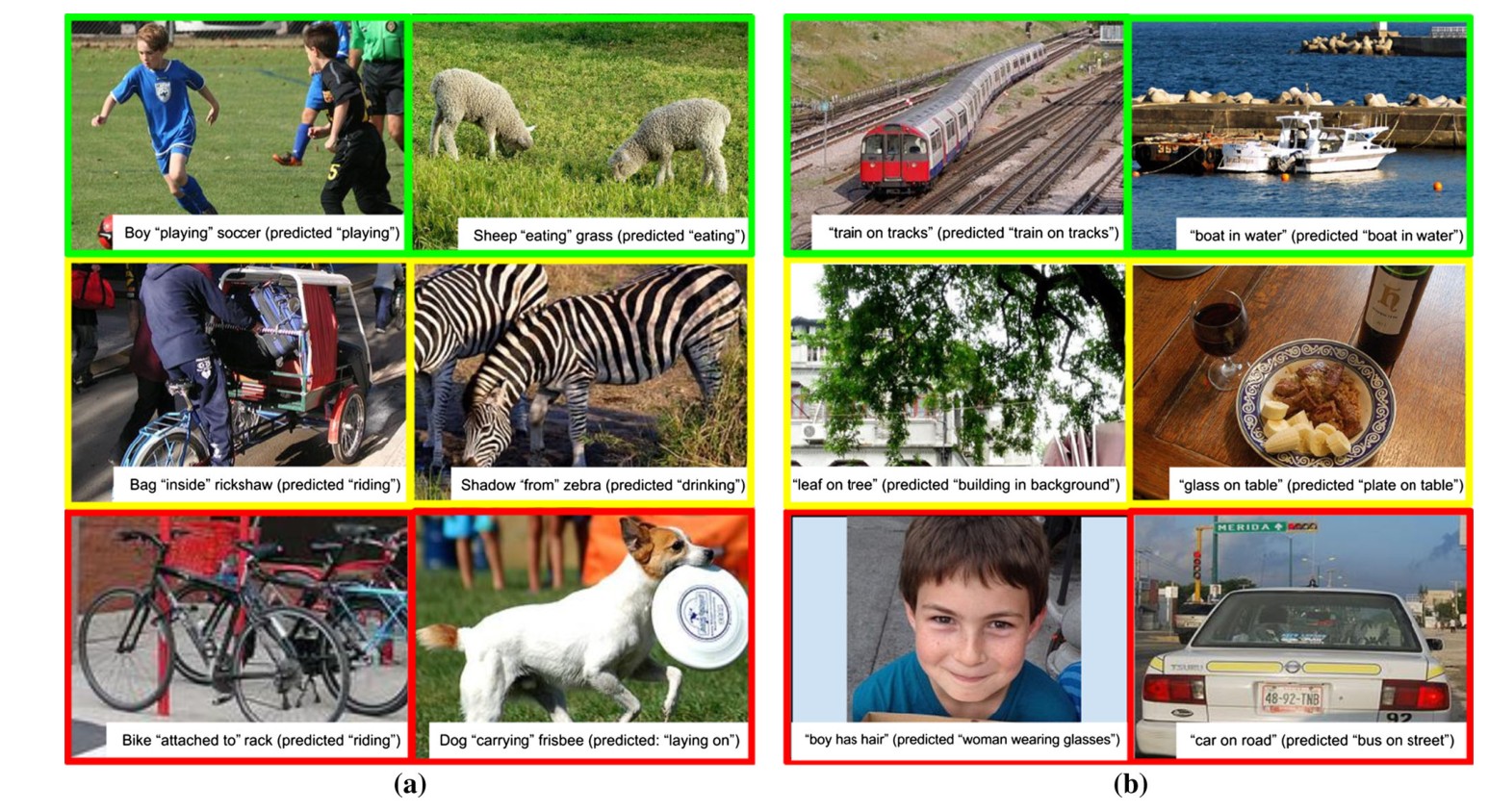
Fig. 36 a Example predictions from the relationship prediction experiment. Relationships in the first row are predicted correctly, those in the second row differ from the ground truth but still correctly classify a relationship in the image, and those in the third row are classified incorrectly. The model learns to associate animals leaning towards the ground as eating or drinking and bikes with riding. b Example predictions from the relationship-objects prediction experiment. The figure is organized in the same way as a. The model is able to predict the salient features of the image but fails to distinguish between different objects (e.g. boy and woman and car and bus in the bottom row)
图 36 a 关系预测实验中的示例预测。第一行关系预测正确,第二行与真值不同但仍然正确分类了图中的一种关系,第三行分类错误。模型会把俯向地面的动物与 eating 或 drinking 联系起来,把自行车与 riding 联系起来。b 关系–物体预测实验中的示例预测。图的组织方式与 a 相同。模型能够预测图像中的显著特征,但无法区分不同物体(例如 底行 中的 boy 与 woman,以及 car 与 bus)。
Results Overall, we find that relationships are only slightly visually distinct enough for our discriminative model to learn effectively. Table 7 shows results for both experiments. For relationship classification, we converge after around 800 iterations with top-one accuracy and top-five accuracy. Unlike attribute prediction, the accuracy results for relationships are much lower because of the high intra-class variability of most relationships. For the second experiment jointly predicting the relationship and its two object classes, we converge after around 450 iterations with top-one accuracy and top-five accuracy. We notice that object classification aids relationship prediction. Some relationships occur with some objects and never others; for example, the relationship drive only occurs with the object person and never with any other objects (dog, chair, etc.).
结果 总体而言,我们发现关系在视觉上只具有勉强足以让我们的判别模型有效学习的区分度。表 7 给出两项实验的结果。在关系分类中,我们大约在 800 次迭代后收敛,top-1 准确率为 ,top-5 准确率为 。与属性预测不同,关系上的准确率要低得多,因为大多数关系的类内可变性很高。在联合预测关系及其两个物体类别的第二项实验中,我们大约在 450 次迭代后收敛,top-1 准确率为 ,top-5 准确率为 。我们注意到,物体分类有助于关系预测。有些关系只与某些物体一同出现,而从不与其他物体一起出现;例如,关系 drive 只与物体 person 一起出现,而从不与任何其他物体(dog、chair 等)一起出现。
Figure 36a shows example predictions for the relationship classification experiment. In general, the model associates object categories with certain relationships (e.g. animals with eating or drinking, bikes with riding, and kids with playing).
图 36a 给出关系分类实验的示例预测。总体而言,模型会把物体类别与某些关系联系起来(例如动物与 eating 或 drinking,自行车与 riding,孩子与 playing)。
Figure 36b, structured as in Fig. 36a, shows example predictions for the joint prediction of relationships with its objects. The model is able to predict the salient features of the image (e.g. “boat in water”) but fails to distinguish between different objects (e.g. boy vs. woman and car vs. bus in the bottom row).
图 36b 的结构与图 36a 相同,给出了把关系与其物体联合预测的示例。模型能够预测图像中的显著特征(例如“boat in water”),但无法区分不同的物体(例如 底行 中的 boy 与 woman,以及 car 与 bus)。
Table 7 Results for relationship classification (first row) and joint classification (second row) experiments
| Top-1 accuracy (%) | Top-5 accuracy (%) | |
|---|---|---|
| Relationship | 8.74 | 26.69 |
| Sub./Rel./Obj. | 25.83 | 65.57 |
表 7 关系分类(第一行)和联合分类(第二行)实验的结果
| Top-1 准确率(%) | Top-5 准确率(%) | |
|---|---|---|
| 关系 | 8.74 | 26.69 |
| 主语/关系/宾语 | 25.83 | 65.57 |
6.3 Generating Region Descriptions
6.3 生成区域描述
Generating sentence descriptions of images has gained popularity as a task in computer vision (Kiros et al. 2014; Mao et al. 2014; Karpathy and Fei-Fei 2015; Vinyals et al. 2015); however, current state-of-the-art models fail to describe all the different events captured in an image and instead provide only a high-level summary of the image. In this section, we test how well state-of-the-art models can caption the details of images. For both experiments, we use the NeuralTalk model (Karpathy and Fei-Fei 2015), since it not only provides state-of-the-art results but also is shown to be robust enough for predicting short descriptions. We train NeuralTalk on the Visual Genome dataset for region descriptions and on Flickr30K (Young et al. 2014) for full sentence descriptions. As a model trained on other datasets would generate complete sentences and would not be comparable (Chen et al. 2015) to our region descriptions, we convert all region descriptions generated by our model into complete sentences using predefined templates (Hou et al. 2002).
为图像生成句子描述,已在计算机视觉中成为一项流行任务(Kiros et al. 2014; Mao et al. 2014; Karpathy and Fei-Fei 2015; Vinyals et al. 2015);不过,当前最先进的模型无法描述一幅图中捕获到的全部不同事件,而往往只给出对图像的高层摘要。在本节中,我们测试最先进的模型能在多大程度上为图像的细节配文。两项实验都使用 NeuralTalk 模型(Karpathy and Fei-Fei 2015),因为它不仅能给出最先进的结果,而且被表明对于预测短描述足够稳健。我们在 Visual Genome 数据集上训练 NeuralTalk 以生成区域描述,在 Flickr30K(Young et al. 2014)上训练以生成完整句子描述。由于在其他数据集上训练的模型会生成完整句子,因而无法与我们的区域描述相比较(Chen et al. 2015),我们使用预定义模板,把模型生成的全部区域描述转换成完整句子(Hou et al. 2002)。
Setup For training, we begin by preprocessing region descriptions; we remove all non-alphanumeric characters and lowercase and strip excess whitespace from them. We have region descriptions in total. We end up with 3, 784, 857 region descriptions for training – 811, 040 each for validation and testing. Note that we ensure descriptions of regions from the same image are exclusively in the training, validation, or testing set. We feed the bounding boxes of the regions through the pretrained VGG 16-layer network (Simonyan and Zisserman 2014) to get the 4096-dimensional feature vectors of each region. We then use the NeuralTalk (Karpathy and Fei-Fei 2015) model to train a long short-term memory (LSTM) network (Hochreiter and Schmidhuber 1997) to generate descriptions of regions. We use a learning rate of 0.001 trained with rmsprop (Dauphin et al. 2015). The model converges after four days.
实验设置 在训练时,我们先对区域描述做预处理:去掉全部非字母数字字符,并做小写化和去掉多余空白。我们总共有 条区域描述。最终用于训练的区域描述有 3,784,857 条,验证和测试各 811,040 条。需要注意,我们确保来自同一张图的区域描述只出现在训练集、验证集或测试集中的一个里。我们把区域的边界框送入预训练的 VGG 16 层网络(Simonyan and Zisserman 2014),得到每个区域的 4096 维特征向量。然后我们使用 NeuralTalk(Karpathy and Fei-Fei 2015)模型,训练一个长短期记忆(LSTM)网络(Hochreiter and Schmidhuber 1997)来生成区域描述。我们使用 0.001 的学习率,并用 rmsprop(Dauphin et al. 2015)训练。模型在四天后收敛。
Table 8 Results for the region description generation experiment
| BLEU-1 | BLEU-2 | BLEU-3 | BLEU-4 | CIDEr | METEOR | Human | |
|---|---|---|---|---|---|---|---|
| Flickr8K | 0.09 | 0.01 | 0.002 | 0.0004 | 0.05 | 0.04 | 1.6% |
| VG | 0.17 | 0.05 | 0.02 | 0.01 | 0.30 | 0.09 | 43.03% |
Scores in the first row are for the region descriptions generated from the NeuralTalk model trained on Flickr8K, and those in the second row are for those generated by the model trained on Visual Genome data. BLEU, CIDEr, and METEOR scores all compare the predicted description to a ground truth in different ways.
表 8 区域描述生成实验的结果
| BLEU-1 | BLEU-2 | BLEU-3 | BLEU-4 | CIDEr | METEOR | 人工 | |
|---|---|---|---|---|---|---|---|
| Flickr8K | 0.09 | 0.01 | 0.002 | 0.0004 | 0.05 | 0.04 | 1.6% |
| VG | 0.17 | 0.05 | 0.02 | 0.01 | 0.30 | 0.09 | 43.03% |
第一行分数来自在 Flickr8K 上训练的 NeuralTalk 模型所生成的区域描述,第二行来自在 Visual Genome 数据上训练的同一模型。BLEU、CIDEr 和 METEOR 都以不同方式把预测描述与真值相比较。
Fig. 37 Example predictions from the region description generation experiment by a model trained on Visual Genome region descriptions. Regions in the first column (left) accurately describe the region, and those in the second column (right) are incorrect and unrelated to the corresponding region
图 37 区域描述生成实验中的示例预测,模型在 Visual Genome 的区域描述上训练。第一列(左)的区域描述准确地描写了该区域,第二列(右)则不正确,且与对应区域无关。
For testing, we crop the ground-truth region bounding boxes of images and extract their 4096-dimensional 16-layer VGG network (Simonyan and Zisserman 2014) features. We then feed these vectors through the pretrained NeuralTalk model to get predictions for region descriptions.
在测试时,我们裁切图像的真值区域边界框,并提取其 4096 维的 16 层 VGG 网络(Simonyan and Zisserman 2014)特征。然后把这些向量送入预训练的 NeuralTalk 模型,得到区域描述的预测。
Results Table 8 shows the results for the experiment. We calculate BLEU (Papineni et al. 2002), CIDEr (Vedantam et al. 2015a), and METEOR (Denkowski and Lavie 2014) scores (Chen et al. 2015) between the generated descriptions and their ground-truth descriptions. In all cases, the model trained on VisualGenome performs better. Moreover, we asked crowd workers to evaluate whether a generated description was correct—we got 1.6 and for models trained on Flickr30K and on Visual Genome, respectively. The large increase in accuracy when the model trained on our data is due to the specificity of our dataset. Our region descriptions are shorter and cover a smaller image area. In comparison, the Flickr30K data are generic descriptions of entire images with multiple events happening in different regions of the image. The model trained on our data is able to make predictions that are more likely to concentrate on the specific part of the image it is looking at, instead of generating a summary description. The objectively low accuracy in both cases illustrates that current models are unable to reason about complex images.
结果 表 8 给出该实验的结果。我们在生成的描述与其真值描述之间计算 BLEU(Papineni et al. 2002)、CIDEr(Vedantam et al. 2015a)和 METEOR(Denkowski and Lavie 2014)分数(Chen et al. 2015)。在所有情形下,在 Visual Genome 上训练的模型都表现更好。此外,我们请众包工人评估生成的描述是否正确——在 Flickr30K 上训练的模型和在 Visual Genome 上训练的模型分别得到 1.6% 和 。在我们的数据上训练的模型准确率大幅提高,是由于我们数据集的针对性。我们的区域描述更短,覆盖的图像面积也更小。相较之下,Flickr30K 的数据是对整张图的泛泛描述,而图中不同区域里同时发生着多件事情。在我们的数据上训练的模型,更有可能把预测集中在它所看的那一块图像上,而不是生成一段摘要式描述。两种情形下客观准确率都不高,这说明当前模型还无法对复杂图像做推理。
Figure 37 shows examples of regions and their predicted descriptions. Since many examples have short descriptions, the predicted descriptions are also short as expected; however, this causes the model to fail to produce more descriptive phrases for regions with multiple objects or with distinctive objects (i.e. objects with many attributes). While we use templates to convert region descriptions into sentences, future work can explore smarter approaches to combine region descriptions and generate a paragraph connecting all the regions into one coherent description.
图 37 给出若干区域及其预测描述的例子。由于许多样例的描述很短,预测描述如预期那样也很短;不过,这会使得模型在面对含有多个物体或具有显著特征的物体(即带有许多属性的物体)的区域时,无法生成更有描述性的短语。虽然我们使用模板把区域描述转换成句子,未来工作可以探索更智能的方法,把区域描述组合起来,并生成把全部区域连成一段连贯描述的段落。
6.4 Question Answering
6.4 问答
Visual Genome is currently the largest dataset of visual question answers with more than million question and answer pairs. Each of our images contains an average of question answer pairs. Answering questions requires a deeper understanding of an image than generic image captioning. Question answering can involve fine-grained recognition (e.g. “What is the breed of the dog?”), object detection (e.g. “Where is the kite in the image?”), activity recognition (e.g. “What is this man doing?”), knowledge base reasoning (e.g. “Is this glass full?”), and common-sense reasoning (e.g. “What street will we be on if we turn right?”).
Visual Genome 目前是规模最大的视觉问答数据集,有超过 万对问答。我们的 张图中,每张平均有 对问答。回答问题需要对图像有比一般图像配文更深的理解。问答可以涉及细粒度识别(例如“What is the breed of the dog?”)、物体检测(例如“Where is the kite in the image?”)、活动识别(例如“What is this man doing?”)、知识库推理(例如“Is this glass full?”)以及常识推理(例如“What street will we be on if we turn right?”)。
By leveraging the detailed annotations in the scene graphs in Visual Genome, we envision building smart models that can answer a myriad of visual questions. While we encourage the construction of smart models, in this paper, we provide some baseline results to help others compare their models.
通过利用 Visual Genome 场景图中的详细标注,我们设想可以构建能够回答大量视觉问题的智能模型。虽然我们鼓励构建智能模型,但在本文中,我们给出一些基准结果,以便他人比较自己的模型。
Setup We split the QA pairs into a training set () and a test set (). We ensure that all images are exclusive to either the training set or the test set. We implement a simple baseline model that relies on answer frequency. The model counts the top k most frequent answers [similar to the ImageNet challenge (Russakovsky et al. 2015)] in the training set as the predictions for all the test questions, where , 500, and 1000. We let a model make k different predictions. We say the model is correct on a QA if one of the k predictions matches exactly with the ground-truth answer. We report the accuracy over all test questions. This evaluation method works well when the answers are short, especially for single-word answers. However, it causes problems when the answers are long phrases and sentences. We also report humans performance [similar to previous work (Antol et al. 2015; Yu et al. 2015)] on these questions by presenting them with the image and the question along with 10 multiple choice answers out of which one of them was the ground truth and the other 9 were randomly chosen from the dataset. Other evaluation methods require word ontologies (Malinowski and Fritz 2014).
实验设置 我们把问答对划分为训练集()和测试集()。我们确保全部图像只属于训练集或测试集中的一个。我们实现了一个依赖答案频率的简单基线模型。该模型把训练集中出现最频繁的前 k 个答案[类似于 ImageNet 挑战赛(Russakovsky et al. 2015)]作为对全部测试问题的预测,其中 、 和 。我们让模型做出 k 个不同的预测。如果这 k 个预测中有一个与真值答案完全匹配,我们就说该模型在这一问答上是正确的。我们报告在全部测试问题上的准确率。当答案较短、尤其是单词语答案时,这种评估方法效果很好。不过,当答案是长短语和句子时,它会带来问题。我们还报告人在这些问题上的表现[类似于先前工作(Antol et al. 2015; Yu et al. 2015)]:把图像和问题连同 10 个选择题答案一起呈现给他们,其中之一是真值,另外 9 个是从数据集中随机选出的。其他评估方法需要词语本体(Malinowski and Fritz 2014)。
Table 9 Baseline QA performances in the 6 different question types
| Top-100 | Top-500 | Top-1000 | Human | |
|---|---|---|---|---|
| What | 0.420 | 0.602 | 0.672 | 0.965 |
| Where | 0.096 | 0.324 | 0.418 | 0.957 |
| When | 0.714 | 0.809 | 0.834 | 0.944 |
| Who | 0.355 | 0.493 | 0.605 | 0.965 |
| Why | 0.034 | 0.118 | 0.187 | 0.927 |
| How | 0.780 | 0.827 | 0.846 | 0.942 |
| Overall | 0.411 | 0.573 | 0.641 | 0.966 |
We report human evaluation as well as a baseline method that predicts the most frequently occurring answer in the dataset.
表 9 六类问题上的基线问答表现
| Top-100 | Top-500 | Top-1000 | 人类 | |
|---|---|---|---|---|
| What | 0.420 | 0.602 | 0.672 | 0.965 |
| Where | 0.096 | 0.324 | 0.418 | 0.957 |
| When | 0.714 | 0.809 | 0.834 | 0.944 |
| Who | 0.355 | 0.493 | 0.605 | 0.965 |
| Why | 0.034 | 0.118 | 0.187 | 0.927 |
| How | 0.780 | 0.827 | 0.846 | 0.942 |
| 总体 | 0.411 | 0.573 | 0.641 | 0.966 |
我们报告了人工评估,以及一个预测数据集中最常见答案的基线方法。
Results Table 9 shows the performance of the open-ended visual question answering task. These baseline results imply the long-tail distribution of the answers. Long-tail distribution is common in existing QA datasets as well (Antol et al. 2015; Malinowski and Fritz 2014). The top 100, 500, and 1000 most frequent answers only cover , , and of the correct answers. In comparison, the corresponding sets of frequent answers in VQA (Antol et al. 2015) cover , , and of the test set answers. The “where” and “why” questions, which tend to involve spatial and common sense reasoning, tend to have more diverse answers and hence perform poorly, with performances of 9.6 and top-100 respectively. The top 1000 frequent answers cover only 41.8 and of the correct answers from these two question types respectively. In comparison, humans perform extremely well in all the questions types achieving an overall accuracy of .
结果 表 9 给出开放式视觉问答任务的表现。这些基准结果表明答案呈长尾分布。长尾分布在现有问答数据集中也很常见(Antol et al. 2015; Malinowski and Fritz 2014)。出现最频繁的前 100、500 和 1000 个答案,分别只覆盖正确答案的 、 和 。相较之下,VQA(Antol et al. 2015)中相应的高频答案集合分别覆盖测试集答案的 、 和 。“where”和“why”问题往往涉及空间推理和常识推理,答案通常也更多样,因而表现较差,top-100 分别为 9.6% 和 。最频繁的前 1000 个答案,分别只覆盖这两类问题正确答案的 41.8% 和 18.7%。相较之下,人在全部问题类型上都表现极好,总体准确率达到 。
7 Future Applications and Directions
7 未来应用与方向
We have analyzed the individual components of this dataset and presented experiments with baseline results for tasks such as attribute classification, relationship classification, description generation, and question answering. There are, however, more applications and experiments for which our dataset can be used. In this section, we note a few potential applications that our dataset can enable.
我们已经分析了该数据集的各个组成部分,并给出了属性分类、关系分类、描述生成和问答等任务的基准实验结果。不过,我们的数据集还可以用于更多的应用和实验。在本节中,我们指出该数据集有可能促成的若干应用。
Dense Image Captioning We have seen numerous image captioning papers (Kiros et al. 2014; Mao et al. 2014; Karpathy and Fei-Fei 2015; Vinyals et al. 2015) that attempt to describe an entire image with a single caption. However, these captions do not exhaustively describe every part of the scene. A natural extension to this application, which the Visual Genome dataset enables, is the ability to create dense captioning models that describe parts of the scene.
稠密图像配文 我们已经看到大量图像配文论文(Kiros et al. 2014; Mao et al. 2014; Karpathy and Fei-Fei 2015; Vinyals et al. 2015)试图用一条配文来描述整张图。不过,这些配文并不能穷尽地描述场景的每一个部分。Visual Genome 数据集使之成为可能的一个自然延伸,是创建能够描述场景局部的稠密配文模型。
Visual Question Answering While visual question answering has been studied as a standalone task (Yu et al. 2015; Ren et al. 2015a; Antol et al. 2015; Gao et al. 2015), we introduce a dataset that combines all of our question answers with descriptions and scene graphs. Future work can build supervised models that utilize various components of Visual Genome to tackle question answering.
视觉问答 虽然视觉问答已被作为一项独立任务加以研究(Yu et al. 2015; Ren et al. 2015a; Antol et al. 2015; Gao et al. 2015),我们推出的数据集把全部问答与描述和场景图结合在一起。未来工作可以构建利用 Visual Genome 各个组成部分的有监督模型,来处理问答。
Image Understanding While we have seen a surge of image captioning (Kiros et al. 2014) and question answering (Antol et al. 2015) models, there has been little work on creating more comprehensive evaluation metrics to measure how well these models are performing. Such models are usually evaluated using BLEU, CIDEr, or METEOR and other similar metrics that do not effectively measure how well these models understand the image (Chen et al. 2015). The Visual Genome scene graphs can be used as a measurement for image understanding. Generated descriptions and answers can be matched against the ground truth scene graph of an image to evaluate its corresponding model.
图像理解 虽然我们已经看到图像配文(Kiros et al. 2014)和问答(Antol et al. 2015)模型的激增,但在创建更全面的评估指标、以衡量这些模型表现如何方面,工作仍然很少。这类模型通常用 BLEU、CIDEr 或 METEOR 以及其他类似指标来评估,而这些指标并不能有效衡量模型对图像的理解程度(Chen et al. 2015)。Visual Genome 的场景图可以用作图像理解的一种度量。生成的描述和答案可以与一幅图的真值场景图相对照,以评估相应的模型。
Relationship Extraction Relationship extraction has been extensively studied in information retrieval and natural language processing (Zhou et al. 2007; GuoDong et al. 2005; Culotta and Sorensen 2004; Socher et al. 2012). Visual Genome is the first large-scale visual relationship dataset. This dataset can be used to study the extraction of visual relationships(Sadeghi et al. 2015) from images, and its interactions between objects can also be used to study action recognition (Yao and Fei-Fei 2010; Ramanathan et al. 2015) and spatial orientation between objects (Gupta et al. 2009; Prest et al. 2012).
关系抽取 关系抽取已在信息检索和自然语言处理中得到广泛研究(Zhou et al. 2007; GuoDong et al. 2005; Culotta and Sorensen 2004; Socher et al. 2012)。Visual Genome 是第一个大规模视觉关系数据集。该数据集可以用来研究从图像中抽取视觉关系(Sadeghi et al. 2015),其中物体之间的互动也可以用来研究动作识别(Yao and Fei-Fei 2010; Ramanathan et al. 2015)以及物体之间的空间方位(Gupta et al. 2009; Prest et al. 2012)。
Semantic Image Retrieval Previous work has already shown that scene graphs can be used to improve semantic image search (Johnson et al. 2015; Schuster et al. 2015). Further methods can be explored using our region descriptions combined with region graphs. Attention-based search methods can also be explored where the area of interest specified by a query is also localized in the retrieved images.
语义图像检索 先前工作已经表明,场景图可以用来改进语义图像搜索(Johnson et al. 2015; Schuster et al. 2015)。还可以结合我们的区域描述与区域图,探索进一步的方法。也可以探索基于注意力的搜索方法,使查询所指定的感兴趣区域也在检索到的图像中被定位出来。
Completing the Set of Annotations While Visual Genome is the most densely annotated visual dataset for cognitive image understanding, it is still not complete. In most images, it is not feasible to collect an exhaustive set of attributes and relationships for every object or pair of objects. This raises two new research questions. In computer vision, we need to develop new evaluation metrics that do not penalize models due to a lack of a complete set of annotations. In human computer interaction, we need to design new interfaces and workflows that incentivize humans to annotate visual common sense.
补全标注集合 虽然 Visual Genome 是目前用于认知图像理解、标注最稠密的视觉数据集,它仍然并不完备。在大多数图像中,为每个物体或每对物体收集穷尽的属性和关系集合并不可行。这提出了两个新的研究问题。在计算机视觉中,我们需要提出新的评估指标,使模型不会因为缺乏完备的标注集合而受到惩罚。在人机交互中,我们需要设计新的界面和工作流程,以激励人去标注视觉常识。
8 Conclusion
8 结论
Visual Genome provides a multi-layered understanding of pictures. It allows for a multi-perspective study of an image, from pixel-level information like objects, to relationships that require further inference, and to even deeper cognitive tasks like question answering. It is a comprehensive dataset for training and benchmarking the next generation of computer vision models. With Visual Genome, we expect these models to develop a broader understanding of our visual world, complementing computers’ capacities to detect objects with abilities to describe those objects and explain their interactions and relationships. Visual Genome is a large formalized knowledge representation for visual understanding and a more complete set of descriptions and question answers that grounds visual concepts to language.
Visual Genome 提供对图片的多层理解。它允许从多个视角研究一幅图,从物体这类像素级信息,到需要进一步推断的关系,再到问答这类更深的认知任务。它是一个用于训练和评测下一代计算机视觉模型的综合数据集。有了 Visual Genome,我们期望这些模型能对我们的视觉世界形成更广的理解,在计算机检测物体的能力之上,补上描述这些物体、并解释其互动与关系的能力。Visual Genome 是一种用于视觉理解的大规模 形式化知识表示,也是一套更 完备的描述和问答,把 视觉概念锚定到语言。
Acknowledgements
致谢
We would like to start by thanking our sponsors: Stanford Computer Science Department, Yahoo Labs, The Brown Institute for Media Innovation, Toyota, Adobe and ONR MURI. Next, we specially thank Michael Stark, Yutian Li, Frederic Ren, Sherman Leung, Michelle Guo and Gavin Mai for their contributions. We thank Carsten Rother from the University of Dresden for facilitating Oliver Groth’s involvement. We also thank all the thousands of crowd workers for their diligent contribution to Visual Genome. Finally, we thank all members of the Stanford Vision Lab and Stanford HCI Group for their useful comments and discussions.
我们首先要感谢资助方:斯坦福计算机科学系、Yahoo Labs、布朗媒体创新研究所、丰田、Adobe 以及 ONR MURI。接下来,我们特别感谢 Michael Stark、Yutian Li、Frederic Ren、Sherman Leung、Michelle Guo 和 Gavin Mai 所做的贡献。我们感谢德累斯顿大学的 Carsten Rother 为 Oliver Groth 的参与提供了便利。我们也感谢数千名众包工人为 Visual Genome 所做的勤勉贡献。最后,我们感谢斯坦福视觉实验室和斯坦福人机交互组的全体成员给出的有益意见和讨论。
Open Access This article is distributed under the terms of the Creative Commons Attribution 4.0 International License (http://creativecommons.org/licenses/by/4.0/), which permits unrestricted use, distribution, and reproduction in any medium, provided you give appropriate credit to the original author(s) and the source, provide a link to the Creative Commons license, and indicate if changes were made.
References
参考文献
Antol, S., Agrawal, A., Lu, J., Mitchell, M., Batra, D., Zitnick, C. L., et al. (2015). VQA: Visual question answering. In International conference on computer vision (ICCV).
Antol, S., Zitnick, C. L., & Parikh, D. (2014). Zero-shot learning via visual abstraction. In European conference on computer vision (pp. 401–416). Springer.
Baker, C. F., Fillmore, C. J., & Lowe, J. B. (1998). The Berkeley framenet project. In Proceedings of the 36th annual meeting of the association for computational linguistics and 17th international conference on computational linguistics—Volume 1, ACL’98 (pp. 86–90). Stroudsburg, PA: Association for Computational Linguistics.
Betteridge, J., Carlson, A., Hong, S. A., Hruschka, E. R, Jr., Law, E. L., Mitchell, T. M., et al. (2009). Toward never ending language learning. In AAAI spring symposium: Learning by reading and learning to read (pp. 1–2).
Bird, S. (2006). NLTK: The natural language toolkit. In Proceedings of the COLING/ACL on interactive presentation sessions (pp. 69–72). Association for Computational Linguistics.
Bruner, J. (1990). Culture and human development: A new look. Human Development, 33(6), 344–355.
Bunescu, R. C., & Mooney, R. J. (2005). A shortest path dependency kernel for relation extraction. In Proceedings of the conference on human language technology and empirical methods in natural language processing (pp. 724–731). Association for Computational Linguistics.
Chang, A. X., Savva, M., & Manning, C. D. (2014). Semantic parsing for text to 3D scene generation. In ACL 2014 (p. 17).
Chen, X., Fang, H., Lin, T.-Y., Vedantam, R., Gupta, S., Dollar, P., et al. (2015). Microsoft COCO captions: Data collection and evaluation server. arXiv:1504.00325.
Chen, X., & Lawrence Zitnick, C. (2015). Mind’s eye: A recurrent visual representation for image caption generation. In Proceedings of the IEEE conference on computer vision and pattern recognition (pp. 2422–2431).
Chen, X., Liu, Z., & Sun, M. (2014). A unified model for word sense representation and disambiguation. In EMNLP (pp. 1025–1035). Citeseer.
Chen, X., Shrivastava, A., & Gupta, A. (2013). Neil: Extracting visual knowledge from web data. In 2013 IEEE international conference on computer vision (ICCV) (pp. 1409–1416). IEEE.
Choi, W., Chao, Y.-W., Pantofaru, C., & Savarese, S. (2013). Understanding indoor scenes using 3D geometric phrases. In 2013 IEEE conference on computer vision and pattern recognition (CVPR) (pp. 33–40). IEEE.
Culotta, A., & Sorensen, J. (2004). Dependency tree kernels for relation extraction. In Proceedings of the 42nd annual meeting on association for computational linguistics (p. 423). Association for Computational Linguistics.
Dauphin, Y., de Vries, H., & Bengio, Y. (2015). Equilibrated adaptive learning rates for non-convex optimization. In Advances in neural information processing systems (pp. 1504–1512).
Deng, J., Dong, W., Socher, R., Li, L.-J., Li, K., & Fei-Fei, L. (2009). Imagenet: A large-scale hierarchical image database. In IEEE conference on computer vision and pattern recognition, 2009 (CVPR 2009) (pp. 248–255). IEEE.
Denkowski, M., & Lavie, A. (2014). Meteor universal: Language specific translation evaluation for any target language. In Proceedings of the ninth workshop on statistical machine translation. Citeseer.
Dollar, P., Wojek, C., Schiele, B., & Perona, P. (2012). Pedestrian detection: An evaluation of the state of the art. IEEE Transactions on Pattern Analysis and Machine Intelligence, 34(4), 743–761.
Donahue, J., Anne Hendricks, L., Guadarrama, S., Rohrbach, M., Venugopalan, S., Saenko, K., et al. (2015). Long-term recurrent convolutional networks for visual recognition and description. In Proceedings of the IEEE conference on computer vision and pattern recognition (pp. 2625–2634).
Everingham, M., Van Gool, L., Williams, C. K., Winn, J., & Zisserman, A. (2010). The pascal visual object classes (VOC) challenge. International Journal of Computer Vision, 88(2), 303–338.
Fang, H., Gupta, S., Iandola, F., Srivastava, R. K., Deng, L., Dollár, P., et al. (2015). From captions to visual concepts and back. In Proceedings of the IEEE conference on computer vision and pattern recognition (pp. 1473–1482).
Farhadi, A., Endres, I., Hoiem, D., & Forsyth, D. (2009). Describing objects by their attributes. In IEEE conference on computer vision and pattern recognition, 2009 (CVPR 2009) (pp. 1778–1785). IEEE.
Farhadi, A., Hejrati, M., Sadeghi, M. A., Young, P., Rashtchian, C., Hockenmaier, J., et al. (2010). Every picture tells a story: Generating sentences from images. In Computer vision–ECCV 2010 (pp. 15–29). Springer.
Fei-Fei, L., Fergus, R., & Perona, P. (2007). Learning generative visual models from few training examples: An incremental bayesian approach tested on 101 object categories. Computer Vision and Image Understanding, 106(1), 59–70.
Ferrari, V., & Zisserman, A. (2007). Learning visual attributes. In Advances in neural information processing systems (pp. 433–440).
Ferrucci, D., Brown, E., Chu-Carroll, J., Fan, J., Gondek, D., Kalyanpur, A. A., et al. (2010). Building watson: An overview of the deepqa project. AI Magazine, 31(3), 59–79.
Firestone, C., & Scholl, B. J. (2015). Cognition does not affect perception: Evaluating the evidence for top-down effects. Behavioral and brain sciences (pp. 1–72).
Forbus, K. D. (1984). Qualitative process theory. Artificial Intelligence, 24(1), 85–168.
Gao, H., Mao, J., Zhou, J., Huang, Z., Wang, L., & Xu, W. (2015). Are you talking to a machine? Dataset and methods for multilingual image question. In Advances in neural information processing systems (pp. 2296–2304).
Geman, D., Geman, S., Hallonquist, N., & Younes, L. (2015). Visual turing test for computer vision systems. Proceedings of the National Academy of Sciences, 112(12), 3618–3623.
Girshick, R. (2015). Fast R-CNN. In Proceedings of the IEEE international conference on computer vision (pp. 1440–1448).
Girshick, R., Donahue, J., Darrell, T., & Malik, J. (2014). Rich feature hierarchies for accurate object detection and semantic segmentation. In 2014 IEEE conference on computer vision and pattern recognition (CVPR) (pp. 580–587). IEEE.
Goering, C., Rodner, E., Freytag, A., & Denzler, J. (2014). Nonparametric part transfer for fine-grained recognition. In 2014 IEEE conference on computer vision and pattern recognition (CVPR) (pp. 2489–2496). IEEE.
Griffin, G., Holub, A., & Perona, P. (2007). Caltech-256 object category dataset. Technical Report 7694.
GuoDong, Z., Jian, S., Jie, Z., & Min, Z. (2005). Exploring various knowledge in relation extraction. In Proceedings of the 43rd annual meeting on association for computational linguistics (pp. 427–434). Association for Computational Linguistics.
Gupta, A., & Davis, L. S. (2008). Beyond nouns: Exploiting prepositions and comparative adjectives for learning visual classifiers. In Computer vision–ECCV 2008 (pp. 16–29). Springer.
Gupta, A., Kembhavi, A., & Davis, L. S. (2009). Observing human–object interactions: Using spatial and functional compatibility for recognition. IEEE Transactions on Pattern Analysis and Machine Intelligence, 31(10), 1775–1789.
Hayes, P. J. (1978). The naive physics manifesto. Geneva: Institut pour les études sémantiques et cognitives/Université de Genève.
Hayes, P. J. (1985). The second naive physics manifesto. Theories of the commonsense world (pp. 1–36).
Hearst, M. A., Dumais, S. T., Osman, E., Platt, J., & Scholkopf, B. (1998). Support vector machines. IEEE Intelligent Systems and their Applications, 13(4), 18–28.
Hochreiter, S., & Schmidhuber, J. (1997). Long short-term memory. Neural Computation, 9(8), 1735–1780.
Hodosh, M., Young, P., & Hockenmaier, J. (2013). Framing image description as a ranking task: Data, models and evaluation metrics. Journal of Artificial Intelligence Research, 47(1), 853–899.
Hou, C.-S. J., Noy, N. F., & Musen, M. A. (2002). A template-based approach toward acquisition of logical sentences. In Intelligent information processing (pp. 77–89). Springer.
Huang, G. B., Mattar, M., Berg, T., & Learned-Miller, E. (2008). Labeled faces in the wild: A database forstudying face recognition in unconstrained environments. In Workshop on faces in ’real-life’ images: Detection, alignment, and recognition.
Isola, P., Lim, J. J., & Adelson, E. H. (2015). Discovering states and transformations in image collections. In Proceedings of the IEEE conference on computer vision and pattern recognition (pp. 1383–1391).
Izadinia, H., Sadeghi, F., & Farhadi, A. (2014). Incorporating scene context and object layout into appearance modeling. In 2014 IEEE conference on computer vision and pattern recognition (CVPR) (pp. 232–239). IEEE.
Johnson, J., Krishna, R., Stark, M., Li, L.-J., Shamma, D. A., Bernstein, M., et al. (2015). Image retrieval using scene graphs. In IEEE conference on computer vision and pattern recognition (CVPR).
Karpathy, A., & Fei-Fei, L. (2015). Deep visual-semantic alignments for generating image descriptions. In Proceedings of the IEEE conference on computer vision and pattern recognition (pp. 3128–3137).
Kiros, R., Salakhutdinov, R., & Zemel, R. (2014). Multimodal neural language models. In Proceedings of the 31st international conference on machine learning (ICML-14) (pp. 595–603).
Krishna, R., Hata, K., Chen, S., Kravitz, J., Shamma, D. A., Fei-Fei, L., et al. (2016). Embracing error to enable rapid crowdsourcing. In CHI’16-SIGCHI conference on human factors in computing system.
Krizhevsky, A., Sutskever, I., & Hinton, G. E. (2012). Imagenet classification with deep convolutional neural networks. In Advances in neural information processing systems (pp. 1097–1105).
Lampert, C. H., Nickisch, H., & Harmeling, S. (2009). Learning to detect unseen object classes by between-class attribute transfer. In IEEE conference on computer vision and pattern recognition, 2009 (CVPR 2009) (pp. 951–958). IEEE.
Leacock, C., Miller, G. A., & Chodorow, M. (1998). Using corpus statistics and wordnet relations for sense identification. Computational Linguistics, 24(1), 147–165.
Lebret, R., Pinheiro, P. O., & Collobert, R. (2015). Phrase-based image captioning. arXiv:1502.03671.
Lin, T.-Y., Maire, M., Belongie, S., Hays, J., Perona, P., Ramanan, D., et al. (2014). Microsoft COCO: Common objects in context. In Computer vision–ECCV 2014 (pp. 740–755). Springer.
Lu, C., Krishna, R., Bernstein, M., & Fei-Fei, L. (2016). Visual relationship detection using language priors. In European conference on computer vision (ECCV). IEEE.
Ma, L., Lu, Z., & Li, H. (2015). Learning to answer questions from image using convolutional neural network. arXiv:1506.00333.
Malinowski, M., & Fritz, M. (2014). A multi-world approach to question answering about real-world scenes based on uncertain input. In Advances in neural information processing systems (pp. 1682–1690).
Malinowski, M., Rohrbach, M., & Fritz, M. (2015). Ask your neurons: A neural-based approach to answering questions about images. In Proceedings of the IEEE international conference on computer vision (pp. 1–9).
Malisiewicz, T., Efros, A., et al. (2008). Recognition by association via learning per-exemplar distances. In IEEE conference on computer vision and pattern recognition, 2008 (CVPR 2008) (pp. 1–8). IEEE.
Manning, C. D., Surdeanu, M., Bauer, J., Finkel, J., Bethard, S. J., & McClosky, D. (2014). The Stanford CoreNLP natural language processing toolkit. In Proceedings of 52nd annual meeting of the association for computational linguistics: system demonstrations (pp. 55–60).
Mao, J., Xu, W., Yang, Y., Wang, J., & Yuille, A. L. (2014). Explain images with multimodal recurrent neural networks. arXiv:1410.1090.
Mihalcea, R., Chklovski, T. A., & Kilgarriff, A. (2004). The senseval-3 English lexical sample task. Association for Computational Linguistics, UNT Digital Library.
Mikolov, T., Chen, K., Corrado, G., & Dean, J. (2013). Efficient estimation of word representations in vector space. arXiv:1301.3781.
Miller, G. A. (1995). Wordnet: a lexical database for english. Communications of the ACM, 38(11), 39–41.
Niu, F., Zhang, C., Ré, C., & Shavlik, J. (2012). Elementary: Large-scale knowledge-base construction via machine learning and statistical inference. International Journal on Semantic Web and Information Systems (IJSWIS), 8(3), 42–73.
Ordonez, V., Kulkarni, G., & Berg, T. L. (2011). Im2text: Describing images using 1 million captioned photographs. In J. Shawe-Taylor, R. Zemel, P. Bartlett, F. Pereira, & K. Weinberger (Eds.), Advances in neural information processing systems (Vol. 24, pp. 1143–1151). Red Hook: Curran Associates, Inc.
Pal, A. R., & Saha, D. (2015). Word sense disambiguation: A survey. arXiv:1508.01346.
Papineni, K., Roukos, S., Ward, T., & Zhu, W.-J. (2002). BLEU: A method for automatic evaluation of machine translation. In Proceedings of the 40th annual meeting on association for computational linguistics (pp. 311–318). Association for Computational Linguistics.
Patterson, G., Xu, C., Su, H., & Hays, J. (2014). The sun attribute database: Beyond categories for deeper scene understanding. International Journal of Computer Vision, 108(1–2), 59–81.
Perronnin, F., Sánchez, J., & Mensink, T. (2010). Improving the fisher kernel for large-scale image classification. In Computer vision–ECCV 2010 (pp. 143–156). Springer.
Prest, A., Schmid, C., & Ferrari, V. (2012). Weakly supervised learning of interactions between humans and objects. IEEE Transactions on Pattern Analysis and Machine Intelligence, 34(3), 601–614.
Ramanathan, V., Li, C., Deng, J., Han, W., Li, Z., Gu, K., et al. (2015). Learning semantic relationships for better action retrieval in images. In Proceedings of the IEEE conference on computer vision and pattern recognition (pp. 1100–1109).
Ren, M., Kiros, R., & Zemel, R. (2015a). Image question answering: A visual semantic embedding model and a new dataset. arXiv:1505.02074.
Ren, S., He, K., Girshick, R., & Sun, J. (2015b). Faster r-cnn: Towards real-time object detection with region proposal networks. In Advances in neural information processing systems (pp. 91–99).
Ronchi, M. R., & Perona, P. (2015). Describing common human visual actions in images. In X. Xie, M. W. Jones, & G. K. L. Tam (Eds.), Proceedings of the British machine vision conference (BMVC 2015) (pp. 52.1–52.12). BMVA Press.
Rothe, S., & Schütze, H. (2015). Autoextend: Extending word embeddings to embeddings for synsets and lexemes. arXiv:1507.01127.
Russakovsky, O., Deng, J., Su, H., Krause, J., Satheesh, S., Ma, S., et al. (2015). ImageNet large scale visual recognition challenge. International journal of computer vision (IJCV) (pp. 1–42).
Russell, B. C., Torralba, A., Murphy, K. P., & Freeman, W. T. (2008). Labelme: A database and web-based tool for image annotation. International Journal of Computer Vision, 77(1–3), 157–173.
Sadeghi, F., Divvala, S. K., & Farhadi, A. (2015). Viske: Visual knowledge extraction and question answering by visual verification of relation phrases. In Proceedings of the IEEE conference on computer vision and pattern recognition (pp. 1456–1464).
Sadeghi, M. A., & Farhadi, A. (2011). Recognition using visual phrases. In 2011 IEEE conference on computer vision and pattern recognition (CVPR) (pp. 1745–1752). IEEE.
Salehi, N., Irani, L. C., & Bernstein, M. S. (2015). We are dynamo: Overcoming stalling and friction in collective action for crowd workers. In Proceedings of the 33rd annual ACM conference on human factors in computing systems (pp. 1621–1630). ACM.
Schank, R. C., & Abelson, R. P. (2013). Scripts, plans, goals, and understanding: An inquiry into human knowledge structures. Hove: Psychology Press.
Schuler, K. K. (2005). VerbNet: A broad-coverage, comprehensive verb lexicon. Ph.D. thesis, University of Pennsylvania, Philadelphia, PA, USA (AAI3179808).
Schuster, S., Krishna, R., Chang, A., Fei-Fei, L., & Manning, C. D. (2015). Generating semantically precise scene graphs from textual descriptions for improved image retrieval. In Proceedings of the fourth workshop on vision and language (pp. 70–80). Citeseer.
Sermanet, P., Eigen, D., Zhang, X., Mathieu, M., Fergus, R., & LeCun, Y. (2013). Overfeat: Integrated recognition, localization and detection using convolutional networks. arXiv:1312.6229.
Silberman, N., Hoiem, D., Kohli, P., & Fergus, R. (2012). Indoor segmentation and support inference from RGBD images. In ECCV.
Simonyan, K., & Zisserman, A. (2014). Very deep convolutional networks for large-scale image recognition. arXiv:1409.1556.
Snow, R., O’Connor, B., Jurafsky, D., & Ng, A. Y. (2008). Cheap and fast—But is it good?: Evaluating non-expert annotations for natural language tasks. In Proceedings of the conference on empirical methods in natural language processing (pp. 254–263). Association for Computational Linguistics.
Socher, R., Huval, B., Manning, C. D., & Ng, A. Y. (2012). Semantic compositionality through recursive matrix-vector spaces. In Proceedings of the 2012 joint conference on empirical methods in natural language processing and computational natural language learning (pp. 1201–1211). Association for Computational Linguistics.
Steinbach, M., Karypis, G., Kumar, V., et al. (2000). A comparison of document clustering techniques. In KDD workshop on text mining, Boston (Vol. 400, pp. 525–526).
Szegedy, C., Liu, W., Jia, Y., Sermanet, P., Reed, S., Anguelov, D., et al. (2015). Going deeper with convolutions. In Proceedings of the IEEE conference on computer vision and pattern recognition (pp. 1–9).
Thomee, B., Shamma, D. A., Friedland, G., Elizalde, B., Ni, K., Poland, D., et al. (2016). YFCC100M: The new data in multimedia research. Communications of the ACM, 59(2), 64–73.
Torralba, A., Fergus, R., & Freeman, W. T. (2008). 80 million tiny images: A large data set for nonparametric object and scene recognition. IEEE Transactions on Pattern Analysis and Machine Intelligence, 30(11), 1958–1970.
Varma, M., & Zisserman, A. (2005). A statistical approach to texture classification from single images. International Journal of Computer Vision, 62(1–2), 61–81.
Vedantam, R., Lawrence Zitnick, C., & Parikh, D. (2015a). Cider: Consensus-based image description evaluation. In Proceedings of the IEEE conference on computer vision and pattern recognition (pp. 4566–4575).
Vedantam, R., Lin, X., Batra, T., Lawrence Zitnick, C., & Parikh, D. (2015b). Learning common sense through visual abstraction. In Proceedings of the IEEE international conference on computer vision (pp. 2542–2550).
Vinyals, O., Toshev, A., Bengio, S., & Erhan, D. (2015). Show and tell: A neural image caption generator. In Proceedings of the IEEE conference on computer vision and pattern recognition (pp. 3156–3164).
Wah, C., Branson, S., Welinder, P., Perona, P., & Belongie, S. (2011). The Caltech-UCSD birds-200-2011 dataset. Technical Report CNS-TR-2011-001, California Institute of Technology.
Xiao, J., Hays, J., Ehinger, K., Oliva, A., Torralba, A., et al. (2010). Sun database: Large-scale scene recognition from abbey to zoo. In 2010 IEEE conference on computer vision and pattern recognition (CVPR) (pp. 3485–3492). IEEE.
Xu, K., Ba, J., Kiros, R., Cho, K., Courville, A. C., Salakhutdinov, R., Zemel, R. S., and Bengio, Y. (2015). Show, attend and tell: Neural image caption generation with visual attention. CoRR. arXiv:1502.03044.
Yang, Y., Baker, S., Kannan, A., & Ramanan, D. (2012). Recognizing proxemics in personal photos. In 2012 IEEE conference on computer vision and pattern recognition (CVPR) (pp. 3522–3529). IEEE.
Yao, B., & Fei-Fei, L. (2010). Modeling mutual context of object and human pose in human–object interaction activities. In 2010 IEEE conference on computer vision and pattern recognition (CVPR) (pp. 17–24). IEEE.
Yao, B., Yang, X., & Zhu, S.-C. (2007). Introduction to a large-scale general purpose ground truth database: methodology, annotation tool and benchmarks. In Energy minimization methods in computer vision and pattern recognition (pp. 169–183). Springer.
Young, P., Lai, A., Hodosh, M., & Hockenmaier, J. (2014). From image descriptions to visual denotations: New similarity metrics for semantic inference over event descriptions. Transactions of the Association for Computational Linguistics, 2, 67–78.
Yu, L., Park, E., Berg, A. C., & Berg, T. L. (2015). Visual madlibs: Fill in the blank image generation and question answering. arXiv:1506.00278.
Zeng, D., Liu, K., Lai, S., Zhou, G., & Zhao, J. (2014). Relation classification via convolutional deep neural network. In Proceedings of COLING (pp. 2335–2344).
Zhou, G., Zhang, M., Ji, D. H., & Zhu, Q. (2007). Tree kernel-based relation extraction with context-sensitive structured parse tree information. In EMNLP-CoNLL 2007 (p. 728).
Zhu, J., Nie, Z., Liu, X., Zhang, B., & Wen, J.-R. (2009). Statsnowball: A statistical approach to extracting entity relationships. In Proceedings of the 18th international conference on world wide web (pp. 101–110). ACM.
Zhu, Y., Fathi, A., & Fei-Fei, L. (2014). Reasoning about object affordances in a knowledge base representation. In European conference on computer vision.
Zhu, Y., Zhang, C., Ré, C., & Fei-Fei, L. (2015). Building a large-scale multimodal knowledge base system for answering visual queries. arXiv:1507.05670.
Zitnick, C. L., & Parikh, D. (2013). Bringing semantics into focus using visual abstraction. In 2013 IEEE conference on computer vision and pattern recognition (CVPR) (pp. 3009–3016). IEEE.