VINS-Mono: A Robust and Versatile Monocular Visual-Inertial State Estimator

VINS-Mono：一种稳健而通用的单目视觉惯性状态估计器

Tong Qin    Peiliang Li    Shaojie Shen † † thanks: T. Qin, P. Li, and S. Shen are with the Department of Electronic and Computer Engineering, Hong Kong University of Science and Technology. e-mail: {tqinab, pliap}@connect.ust.hk, eeshaojie@ust.hk

Abstract

摘要

A monocular visual-inertial system (VINS), consisting of a camera and a low-cost inertial measurement unit (IMU), forms the minimum sensor suite for metric six degrees-of-freedom (DOF) state estimation. However, the lack of direct distance measurement poses significant challenges in terms of IMU processing, estimator initialization, extrinsic calibration, and nonlinear optimization. In this work, we present VINS-Mono: a robust and versatile monocular visual-inertial state estimator. Our approach starts with a robust procedure for estimator initialization and failure recovery. A tightly-coupled, nonlinear optimization-based method is used to obtain high accuracy visual-inertial odometry by fusing pre-integrated IMU measurements and feature observations. A loop detection module, in combination with our tightly-coupled formulation, enables relocalization with minimum computation overhead. We additionally perform four degrees-of-freedom pose graph optimization to enforce global consistency. We validate the performance of our system on public datasets and real-world experiments and compare against other state-of-the-art algorithms. We also perform onboard closed-loop autonomous flight on the MAV platform and port the algorithm to an iOS-based demonstration. We highlight that the proposed work is a reliable, complete, and versatile system that is applicable for different applications that require high accuracy localization. We open source our implementations for both PCs[^1] and iOS mobile devices[^2].

由一台相机和一块低成本惯性测量单元（IMU）组成的单目视觉惯性系统（VINS），是做带度量尺度的六自由度（DOF）状态估计所需的最小传感器组合。然而，由于缺少直接的距离测量，IMU 处理、估计器初始化、外参标定和非线性优化都面临明显挑战。本文提出 VINS-Mono：一种稳健而通用的单目视觉惯性状态估计器。方法从一套稳健的估计器初始化与故障恢复流程开始。随后用紧耦合、基于非线性优化的方法，融合预积分的 IMU 测量与特征观测，得到高精度的视觉惯性里程计。再配合回环检测模块，以及我们的紧耦合表述，可以在计算开销很小的情况下完成重定位。我们另外做四自由度位姿图优化，以施加全局一致性。我们在公开数据集和真实实验上验证了系统表现，并与其他当时最好的算法做了比较。我们还在微型飞行器（MAV）平台上做了机载闭环自主飞行，并把算法移植到基于 iOS 的演示中。需要强调的是，这项工作是一套可靠、完整且通用的系统，适用于多种对定位精度要求很高的应用。我们开源了面向个人电脑和 iOS 移动设备的实现。

Index Terms: Monocular visual-inertial systems, state estimation, sensor fusion, simultaneous localization and mapping

索引词：单目视觉惯性系统（Monocular visual-inertial systems），状态估计（state estimation），传感器融合（sensor fusion），同时定位与建图（simultaneous localization and mapping）

I Introduction

I 引言

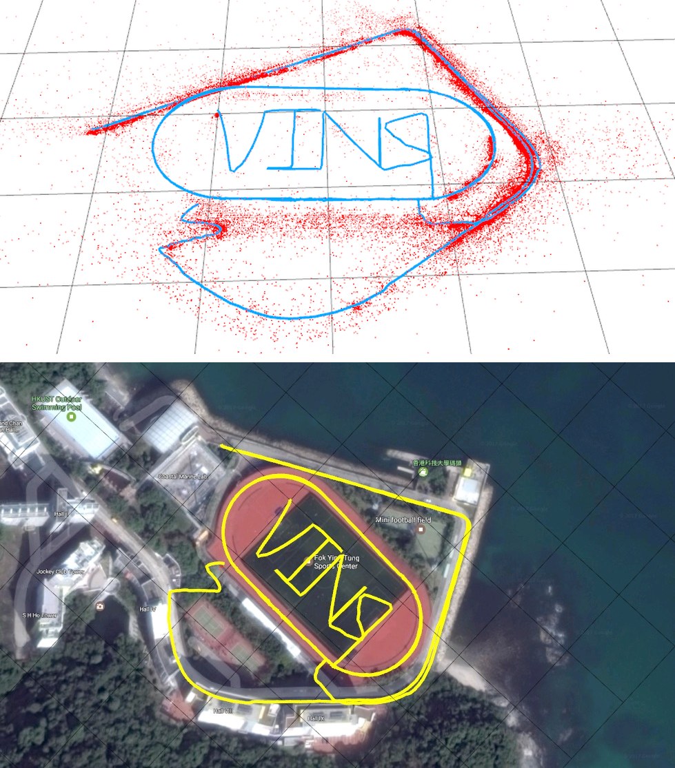
Fig. 1: Outdoor experimental results of the proposed monocular visual-inertial state estimator. Data is collected by a hand-held monocular camera-IMU setup under normal walking condition. It includes two complete circles inside the field and two semicircles on the nearby driveway. Total trajectory length is 2.5 km. A video of the experiment can be found in the multimedia attachment.

(a) Trajectory (blue) and feature locations (red)
(b) Trajectory overlaid with Google Map for visual comparison

图 1：所提出的单目视觉惯性状态估计器的室外实验结果。数据由手持的单目相机-IMU 装置在正常步行条件下采集，包含场地内的两整圈，以及附近车道上的两段半圆。轨迹总长 2.5 公里。实验视频见多媒体附件。

(a) 轨迹（蓝）与特征位置（红）
(b) 叠在 Google 地图上便于对照的轨迹

State estimation is undoubtedly the most fundamental module for a wide range of applications, such as robotic navigation, autonomous driving, virtual reality (VR), and augmented reality (AR). Approaches that use only a monocular camera have gained significant interests by the community due to their small size, low-cost, and easy hardware setup [1, 2, 3, 4, 5]. However, monocular vision-only systems are incapable of recovering the metric scale, therefore limiting their usage in real-world robotic applications. Recently, we see a growing trend of assisting the monocular vision system with a low-cost inertial measurement unit (IMU). The primary advantage of this monocular visual-inertial system (VINS) is to have the metric scale, as well as roll and pitch angles, all observable. This enables navigation tasks that require metric state estimates. In addition, the integration of IMU measurements can dramatically improve motion tracking performance by bridging the gap between losses of visual tracks due to illumination change, texture-less area, or motion blur. In fact, the monocular VINS not only widely available on mobile robots, drones, and mobile devices, it is also the minimum sensor setup for sufficient self and environmental perception.

状态估计无疑是机器人导航、自动驾驶、虚拟现实（VR）和增强现实（AR）等广泛应用中最基础的模块。只用单目相机的方法因其体积小、成本低、硬件设置简单，在社区中受到了很大关注[1, 2, 3, 4, 5]。然而，纯单目视觉系统无法恢复度量尺度，因而限制了它在真实机器人应用中的使用。近来，用一块低成本惯性测量单元（IMU）来辅助单目视觉系统的做法越来越常见。这种单目视觉惯性系统（VINS）的主要好处是，度量尺度以及横滚角和俯仰角都是可观测的。这使需要度量状态估计的导航任务成为可能。此外，对 IMU 测量做积分，还能在光照变化、弱纹理或运动模糊造成视觉跟踪丢失时把空隙补上，从而显著改善运动跟踪。事实上，单目 VINS 不仅在移动机器人、无人机和移动设备上已经广泛可用，它也是完成自身与环境感知所需的最小传感器组合。

However, all these advantages come with a price. For monocular VINS, it is well known that acceleration excitation is needed to make metric scale observable. This implies that monocular VINS estimators cannot start from a stationary condition, but rather launch from an unknown moving state. Also recognizing the fact that visual-inertial systems are highly nonlinear, we see significant challenges in terms of estimator initialization. The existence of two sensors also makes camera-IMU extrinsic calibration critical. Finally, in order to eliminate long-term drift within an acceptable processing window, a complete system that includes visual-inertial odometry, loop detection, relocalization, and global optimization has to be developed.

不过，这些好处是有代价的。对单目 VINS 而言，众所周知需要加速度激励，尺度才可观测。这意味着单目 VINS 估计器不能从静止状态起步，而要从未知的运动状态启动。再加上视觉惯性系统高度非线性，估计器初始化就成了显著挑战。两种传感器并存，也使相机-IMU 外参标定变得关键。最后，要在可接受的处理窗口内消除长期漂移，还必须做成一套包含视觉惯性里程计、回环检测、重定位和全局优化的完整系统。

To address all these issues, we propose VINS-Mono, a robust and versatile monocular visual-inertial state estimator. Our solution starts with on-the-fly estimator initialization. The same initialization module is also used for failure recovery. The core of our solution is a robust monocular visual-inertial odometry (VIO) based on tightly-coupled sliding window nonlinear optimization. The monocular VIO module not only provides accurate local pose, velocity, and orientation estimates, it also performs camera-IMU extrinsic calibration and IMU biases correction in an online fashion. Loops are detected using DBoW2 [6]. Relocalization is done in a tightly-coupled setting by feature-level fusion with the monocular VIO. This enables robust and accurate relocalization with minimum computation overhead. Finally, geometrically verified loops are added into a pose graph, and thanks to the observable roll and pitch angles from the monocular VIO, a four degrees-of-freedom (DOF) pose graph is performed to ensure global consistency.

为应对这些问题，我们提出 VINS-Mono，一种稳健而通用的单目视觉惯性状态估计器。方案从在线的估计器初始化开始，同一套初始化模块也用于故障恢复。方案的核心，是基于紧耦合滑动窗口非线性优化的稳健单目视觉惯性里程计（VIO）。单目 VIO 模块不仅给出准确的局部位姿、速度和姿态估计，还在线完成相机-IMU 外参标定和 IMU 偏置校正。回环用 DBoW2[6] 检测。重定位在紧耦合设定下、通过与单目 VIO 的特征级融合完成。这样可以在计算开销很小的情况下，得到稳健而准确的重定位。最后，几何上得到验证的回环被加入位姿图；得益于单目 VIO 使横滚和俯仰可观测，我们做四自由度（DOF）位姿图优化，以保证全局一致性。

VINS-Mono combines and improves the our previous works on monocular visual-inertial fusion [7, 8, 9, 10]. It is built on top our tightly-coupled, optimization-based formulation for monocular VIO [7, 8], and incorporates the improved initialization procedure introduced in [9]. The first attempt of porting to mobile devices was given in [10]. Further improvements of VINS-Mono comparing to our previous works include improved IMU pre-integration with bias correction, tightly-coupled relocalization, global pose graph optimization, extensive experimental evaluation, and a robust and versatile open source implementation.

VINS-Mono 综合并改进了我们先前在单目视觉惯性融合上的工作[7, 8, 9, 10]。它建立在我们紧耦合、基于优化的单目 VIO 表述[7, 8]之上，并纳入了[9]中改进的初始化流程。向移动设备移植的第一次尝试见[10]。与先前工作相比，VINS-Mono 的进一步改进包括：带偏置校正的改进 IMU 预积分、紧耦合重定位、全局位姿图优化、广泛的实验评估，以及一套稳健而通用的开源实现。

The whole system is complete and easy-to-use. It has been successfully applied to small-scale AR scenarios, medium-scale drone navigation, and large-scale state estimation tasks. Superior performance has been shown against other state-of-the-art methods. To this end, we summarize our contributions as follow:

整套系统完整且易于使用。它已成功用于小尺度 AR 场景、中等尺度无人机导航，以及大尺度状态估计任务，并相对其他当时最好的方法表现出更优的性能。为此，我们将贡献概括如下：

• • A robust initialization procedure that is able to bootstrap the system from unknown initial states.

• 一套稳健的初始化流程，能够从未知初始状态把系统启动起来。

• • A tightly-coupled, optimization-based monocular visual-inertial odometry with camera-IMU extrinsic calibration and IMU bias estimation.

• 紧耦合、基于优化的单目视觉惯性里程计，同时进行相机-IMU 外参标定和 IMU 偏置估计。

• • Online loop detection and tightly-coupled relocalization.

• 在线回环检测与紧耦合重定位。

• • Four DOF global pose graph optimization.

• 四自由度全局位姿图优化。

• • Real-time performance demonstration for drone navigation, large-scale localization, and mobile AR applications.

• 在无人机导航、大尺度定位和移动 AR 应用中的实时性能演示。

• • Open-source release for both the PC version that is fully integrated with ROS, as well as the iOS version that runs on iPhone6s or above.

• 开源发布：与 ROS 完整集成的电脑版本，以及可在 iPhone 6s 及以上机型上运行的 iOS 版本。

The rest of the paper is structured as follows. In Sect. II, we discuss relevant literature. We give an overview of the complete system pipeline in Sect. III. Preprocessing steps for both visual and pre-integrated IMU measurements are presented in Sect. IV. In Sect. V, we discuss the estimator initialization procedure. A tightly-coupled, self-calibrating, nonlinear optimization-based monocular VIO, is presented in Sect. VI. Tightly-coupled relocalization and global pose graph optimization are presented in Sect. VII and Sect. VIII respectively. Implementation details and experimental results are shown in Sect. IX. Finally, the paper is concluded with a discussion and possible future research directions in Sect. X.

后文结构如下。第 II 节讨论相关文献。第 III 节给出完整系统流程的概览。第 IV 节介绍视觉测量与预积分 IMU 测量的预处理。第 V 节讨论估计器初始化流程。第 VI 节给出紧耦合、可自标定、基于非线性优化的单目 VIO。紧耦合重定位和全局位姿图优化分别在第 VII 节和第 VIII 节介绍。实现细节与实验结果见第 IX 节。最后，第 X 节总结全文，并讨论可能的后续研究方向。

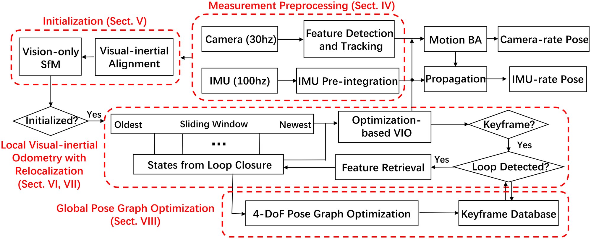
Fig. 2: A block diagram illustrating the full pipeline of the proposed monocular visual-inertial state estimator.

图 2：所提出的单目视觉惯性状态估计器完整流程的框图。

II Related Work

II 相关工作

Scholarly works on monocular vision-based state estimation/odometry/SLAM are extensive. Noticeable approaches include PTAM [1], SVO [2], LSD-SLAM [3], DSO [5], and ORB-SLAM [4]. It is obvious that any attempts to give a full relevant review would be incomplete. In this section, however, we skip the discussion on vision-only approaches, and only focus on the most relevant results on monocular visual-inertial state estimation.

关于单目视觉状态估计、里程计和 SLAM 的文献非常多。值得注意的方法包括 PTAM[1]、SVO[2]、LSD-SLAM[3]、DSO[5] 和 ORB-SLAM[4]。任何试图给出完整综述的做法显然都会有遗漏。不过在本节中，我们略过纯视觉方法的讨论，只聚焦与单目视觉惯性状态估计最相关的结果。

The simplest way to deal with visual and inertial measurements is loosely-coupled sensor fusion [11, 12], where IMU is treated as an independent module to assist vision-only pose estimates obtained from the visual structure from motion. Fusion is usually done by an extended Kalman filter (EKF), where IMU is used for state propagation and the vision-only pose is used for the update. Further on, tightly-coupled visual-inertial algorithms are either based on the EKF [13, 14, 15] or graph optimization [16, 7, 8, 17], where camera and IMU measurements are jointly optimized from the raw measurement level. A popular EKF based VIO approach is MSCKF [13, 14]. MSCKF maintains several previous camera poses in the state vector, and uses visual measurements of the same feature across multiple camera views to form multi-constraint update. SR-ISWF [18, 19] is an extension of MSCKF. It uses square-root form [20] to achieve single-precision representation and avoid poor numerical properties. This approach employs the inverse filter for iterative re-linearization, making it equal to optimization-based algorithms. Batch graph optimization or bundle adjustment techniques maintain and optimize all measurements to obtain the optimal state estimates. To achieve constant processing time, popular graph-based VIO methods [16, 8, 17] usually optimize over a bounded-size sliding window of recent states by marginalizing out past states and measurements. Due to high computational demands of iterative solving of nonlinear systems, few graph-based can achieve real-time performance on resource-constrained platforms, such as mobile phones.

处理视觉与惯性测量最简单的办法，是松耦合传感器融合[11, 12]：把 IMU 当作独立模块，去辅助由视觉运动恢复结构得到的纯视觉位姿估计。融合通常由扩展卡尔曼滤波（EKF）完成，用 IMU 做状态传播，用纯视觉位姿做更新。更进一步，紧耦合的视觉惯性算法或基于 EKF[13, 14, 15]，或基于图优化[16, 7, 8, 17]，从原始测量层面联合优化相机与 IMU 测量。一种流行的、基于 EKF 的 VIO 方法是 MSCKF[13, 14]。MSCKF 在状态向量中保持若干先前相机位姿，并用同一特征在多个相机视角下的视觉测量构成多约束更新。SR-ISWF[18, 19] 是 MSCKF 的扩展。它采用平方根形式[20]，以实现单精度表示并避免不良数值性质。该方法使用逆滤波器做迭代重新线性化，从而与基于优化的算法等价。批量图优化或光束法平差技术会保持并优化全部测量，以得到最优状态估计。为了达到恒定处理时间，常见的基于图的 VIO 方法[16, 8, 17]通常只在有界大小的近期状态滑动窗口上优化，并把过去的状态和测量边缘化掉。由于迭代求解非线性系统的计算量很大，很少有基于图的方法能在手机这类资源受限平台上达到实时。

For visual measurement processing, algorithms can be categorized into either direct or indirect method according to the definition of visual residual models. Direct approaches [2, 3, 21] minimize photometric error while indirect approaches [16, 8, 14] minimize geometric displacement. Direct methods require a good initial guess due to their small region of attraction, while indirect approaches consume extra computational resources on extracting and matching features. Indirect approaches are more frequently found in real-world engineering deployment due to its maturity and robustness. However, direct approaches are easier to be extended for dense mapping as they are operated directly on the pixel level.

就视觉测量处理而言，可按视觉残差模型的定义，把算法分成直接法或间接法。直接方法[2, 3, 21]最小化光度误差，间接方法[16, 8, 14]最小化几何位移。直接法由于其吸引域较小，需要较好的初值；间接法则要把额外计算花在提取和匹配特征上。由于其成熟和稳健，间接法在真实工程部署中更常见。不过，直接法直接在像素级操作，更容易扩展到稠密建图。

In practice, IMUs usually acquire data at a much higher rate than the camera. Different methods have been proposed to handle the high rate IMU measurements. The most straightforward approach is to use the IMU for state propagation in EKF-based approaches  [11, 13]. In a graph optimization formulation, an efficient technique called IMU pre-integration is developed in order to avoid repeated IMU re-integration This technique was first introduced in [22], which parametrize rotation error using Euler angles. An on-manifold rotation formulation for IMU-preintegration was developed in our previous work [7]. This work derived the covariance propagation using continuous-time IMU error state dynamics. However, IMU biases were ignored. The pre-integration theory was further improved in [23] by adding posterior IMU bias correction.

实践中，IMU 的采样率通常远高于相机。已有多种方法来处理高速率 IMU 测量。最直截的做法，是在基于 EKF 的方法中用 IMU 做状态传播[11, 13]。在图优化表述中，为避免反复对 IMU 重新积分，发展出了一种称为 IMU 预积分的高效技术。该技术最早在[22]中提出，用欧拉角参数化旋转误差。我们先前的工作[7]给出了 IMU 预积分的流形上旋转表述，并用连续时间 IMU 误差状态动力学推导了协方差传播。不过当时忽略了 IMU 偏置。预积分理论随后在[23]中得到进一步改进，加入了后验 IMU 偏置校正。

Accurate initial values are crucial to bootstrap any monocular VINS. A linear estimator initialization method that leverages relative rotations from short-term IMU pre-integration was proposed in [24, 8]. However, this method does not model gyroscope bias, and fails to model sensor noise in raw projection equations. In real-world applications, this results in unreliable initialization when visual features are far away from the sensor suite. A closed-form solution to the monocular visual-inertial initialization problem was introduced in [25]. Later, an extension to this closed-form solution by adding gyroscope bias calibration was proposed in [26]. These approaches fail to model the uncertainty in inertial integration since they rely on the double integration of IMU measurements over an extended period of time. In [27], a re-initialization and failure recovery algorithm based on SVO [2] was proposed. This is a practical method based on a loosely-coupled fusion framework. However, an additional downward-facing distance sensor is required to recover the metric scale. An initialization algorithm built on top of the popular ORB-SLAM [4] was introduced in [17]. An initial estimation of the scale, gravity direction, velocity and IMU biases are computed for the visual-inertial full BA given a set of keyframes from ORB-SLAM. However, it is reported that the time required for scale convergence can be longer than 10 seconds. This can pose problems for robotic navigation tasks that require scale estimates right at the beginning.

准确的初值对启动任何单目 VINS 都至关重要。[24, 8]提出一种线性估计器初始化方法，利用短时 IMU 预积分得到的相对旋转。不过该方法不建模陀螺仪偏置，也没有在原始投影方程中建模传感器噪声。在真实应用中，当视觉特征离传感器组合较远时，这会导致初始化不可靠。[25]给出了单目视觉惯性初始化问题的闭式解。随后，[26]在这一闭式解上做了扩展，加入了陀螺仪偏置标定。这些方法依赖在较长时段上对 IMU 测量做双重积分，因而未能建模惯性积分中的不确定性。[27]提出一种基于 SVO[2] 的重新初始化与故障恢复算法。这是建立在松耦合融合框架上的实用方法，但需要额外的朝下距离传感器才能恢复度量尺度。[17]介绍了一种建立在流行的 ORB-SLAM[4] 之上的初始化算法。给定一组来自 ORB-SLAM 的关键帧，先估计尺度、重力方向、速度和 IMU 偏置，再交给视觉惯性完整 BA。不过据报告，尺度收敛所需时间可能长于 10 秒。这对一开始就需要尺度估计的机器人导航任务会构成问题。

VIO approaches, regardless the underlying mathematical formulation that they rely on, suffer from long term drifting in global translation and orientation. To this end, loop closure plays an important role for long-term operations. ORB-SLAM [4] is able to close loops and reuse the map, which takes advantage of Bag-of-World [6]. A 7 DOF [28] (position, orientation, and scale) pose graph optimization is followed loop detection. In contrast, for monocular VINS, thanks to the addition of IMU, drift only occurs in 4 DOF, which is the 3D translation, and the rotation around the gravity direction (yaw angle). Therefore, in this paper, we choose to optimize the pose graph with loop constraints in the minimum 4 DOF setting.

无论依赖怎样的数学表述，VIO 方法都会在全局平移和朝向上出现长期漂移。因此，回环闭合对长期运行十分重要。ORB-SLAM[4] 能够闭合回环并复用地图，这得益于词袋（Bag-of-Words）[6]。回环检测之后会做 7 自由度[28]（位置、朝向和尺度）的位姿图优化。与此相对，对单目 VINS 而言，由于加入了 IMU，漂移只发生在 4 个自由度上，即三维平移，以及绕重力方向的旋转（偏航角）。因此在本文中，我们选择在最少的 4 自由度设定下，用回环约束优化位姿图。

III Overview

III 概览

The structure of proposed monocular visual-inertial state estimator is shown in Fig. 2. The system starts with measurement preprocessing (Sect. IV), in which features are extracted and tracked, and IMU measurements between two consecutive frames are pre-integrated. The initialization procedure (Sect. V provides all necessary values, including pose, velocity, gravity vector, gyroscope bias, and 3D feature location, for bootstrapping the subsequent nonlinear optimization-based VIO. The VIO (Sect. VI) with relocalization (Sect. VII) modules tightly fuses pre-integrated IMU measurements, feature observations, and re-detected features from loop closure. Finally, the pose graph optimization module (Sect. VIII) takes in geometrically verified relocalization results, and perform global optimization to eliminate drift. The VIO, relocalization, and pose graph optimization modules run concurrently in a multi-thread setting. Each module has different running rates and real-time guarantees to ensure reliable operation at all times.

所提出的单目视觉惯性状态估计器结构如图 2 所示。系统从测量预处理开始（第 IV 节），在这一步提取并跟踪特征，并把相邻两帧之间的 IMU 测量预积分。初始化流程（第 V 节）给出启动后续基于非线性优化的 VIO 所需的全部量，包括位姿、速度、重力向量、陀螺仪偏置和三维特征位置。带重定位（第 VII 节）的 VIO（第 VI 节）紧耦合地融合预积分 IMU 测量、特征观测，以及回环中重新检测到的特征。最后，位姿图优化模块（第 VIII 节）接收经几何验证的重定位结果，并做全局优化以消除漂移。VIO、重定位和位姿图优化模块在多线程设定下并发运行。各模块具有不同的运行频率和实时保证，以确保系统随时可靠工作。

We now define notations and frame definitions that we use throughout the paper. We consider $(\cdot)^{w}$ as the world frame. The direction of the gravity is aligned with the $z$ axis of the world frame. $(\cdot)^{b}$ is the body frame, which we define it to be the same as the IMU frame. $(\cdot)^{c}$ is the camera frame. We use both rotation matrices $\mathbf{R}$ and Hamilton quaternions $\mathbf{q}$ to represent rotation. We primarily use quaternions in state vectors, but rotation matrices are also used for convenience rotation of 3D vectors. $\mathbf{q}^{w}_{b},\mathbf{p}^{w}_{b}$ are rotation and translation from the body frame to the world frame. $b_{k}$ is the body frame while taking the $k^{th}$ image. $c_{k}$ is the camera frame while taking the $k^{th}$ image. $\otimes$ represents the multiplication operation between two quaternions. $\mathbf{g}^{w}=[0,0,g]^{T}$ is the gravity vector in the world frame. Finally, we denote $\hat{(\cdot)}$ as the noisy measurement or estimate of a certain quantity.

下面定义全文使用的记号和坐标系。我们把 $(\cdot)^{w}$ 作为世界系。重力方向与世界系的 $z$ 轴对齐。$(\cdot)^{b}$ 是体系，我们把它定义成与 IMU 坐标系相同。$(\cdot)^{c}$ 是相机系。我们同时用旋转矩阵 $\mathbf{R}$ 和哈密顿四元数 $\mathbf{q}$ 表示旋转。状态向量中主要使用四元数，但为了方便旋转三维向量，也会用旋转矩阵。$\mathbf{q}^{w}_{b},\mathbf{p}^{w}_{b}$ 是从体系到世界系的旋转和平移。$b_{k}$ 是拍摄第 $k$ 张图像时的体系。$c_{k}$ 是拍摄第 $k$ 张图像时的相机系。$\otimes$ 表示两个四元数之间的乘法。$\mathbf{g}^{w}=[0,0,g]^{T}$ 是世界系中的重力向量。最后，我们用 $\hat{(\cdot)}$ 表示某一量的含噪测量或估计。

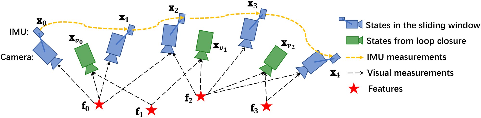
Fig. 3: An illustration of the sliding window monocular VIO with relocalization. It is a tightly-coupled formulation with IMU, visual, and loop measurements.

图 3：带重定位的滑动窗口单目 VIO 示意。这是一种把 IMU、视觉和回环测量紧耦合在一起的表述。

IV Measurement Preprocessing

IV 测量预处理

This section presents preprocessing steps for both inertial and monocular visual measurements. For visual measurements, we track features between consecutive frames and detect new features in the latest frame. For IMU measurements, we pre-integrate them between two consecutive frames. Note that the measurements of the low-cost IMU that we use are affected by both bias and noise. We therefore especially take bias into account in the IMU pre-integration process.

本节介绍惯性测量和单目视觉测量的预处理步骤。对视觉测量，我们在相邻帧之间跟踪特征，并在最新一帧中检测新特征。对 IMU 测量，我们在相邻两帧之间做预积分。需要注意的是，我们使用的低成本 IMU 测量既受偏置影响，也受噪声影响。因此在 IMU 预积分过程中，我们特别把偏置考虑在内。

IV-A Vision Processing Front-end

IV-A 视觉处理前端

For each new image, existing features are tracked by the KLT sparse optical flow algorithm [29]. Meanwhile, new corner features are detected [30] to maintain a minimum number (100-300) of features in each image. The detector enforces a uniform feature distribution by setting a minimum separation of pixels between two neighboring features. 2D Features are firstly undistorted and then projected to a unit sphere after passing outlier rejection. Outlier rejection is performed using RANSAC with fundamental matrix model [31].

对每张新图像，已有特征由 KLT 稀疏光流算法[29]跟踪。与此同时，检测新的角点特征[30]，以在每张图像中维持最低数量（100–300）的特征。检测器通过设定相邻特征之间的最小像素间隔，来强制特征均匀分布。二维特征先去畸变，通过外点剔除后再投影到单位球上。外点剔除使用带基本矩阵模型的 RANSAC[31]。

Keyframes are also selected in this step. We have two criteria for keyframe selection. The first one is the average parallax apart from the previous keyframe. If the average parallax of tracked features is between the current frame and the latest keyframe is beyond a certain threshold, we treat frame as a new keyframe. Note that not only translation but also rotation can cause parallax. However, features cannot be triangulated in the rotation-only motion. To avoid this situation, we use short-term integration of gyroscope measurements to compensate rotation when calculating parallax. Note that this rotation compensation is only used to keyframe selection, and is not involved in rotation calculation in the VINS formulation. To this end, even if the gyroscope contains large noise or is biased, it will only result in suboptimal keyframe selection results, and will not directly affect the estimation quality. Another criterion is tracking quality. If the number of tracked features goes below a certain threshold, we treat this frame as a new keyframe. This criterion is to avoid complete loss of feature tracks.

关键帧也在这一步选取。我们有两条关键帧选取准则。第一条是相对上一关键帧的平均视差。如果当前帧与最近关键帧之间、被跟踪特征的平均视差超过某一阈值，就把该帧当作新关键帧。需要注意，不仅平移、旋转也会造成视差。然而，在纯旋转运动中特征无法被三角化。为避免这种情况，我们在计算视差时用陀螺仪测量的短时积分来补偿旋转。需要说明，这种旋转补偿只用于关键帧选取，并不参与 VINS 表述中的旋转计算。因此，即便陀螺仪噪声很大或存在偏置，也只会导致关键帧选取不够理想，而不会直接损害估计质量。另一条准则是跟踪质量。如果被跟踪特征的数量低于某一阈值，我们也把该帧当作新关键帧。这条准则是为了避免特征跟踪完全丢失。

IV-B IMU Pre-integration

IV-B IMU 预积分

IMU Pre-integration was first proposed in [22], which parametrized rotation error in Euler angle. An on-manifold rotation formulation for IMU pre-integration was developed in our previous work [7]. This work derived the covariance propagation using continuous-time IMU error state dynamics. However, IMU biases were ignored. The pre-integration theory was further improved in [23] by adding posterior IMU bias correction. In this paper, we extend the IMU pre-integration proposed in our previous work [7] by incorporating IMU bias correction.

IMU 预积分最早在[22]中提出，用欧拉角参数化旋转误差。我们先前的工作[7]给出了 IMU 预积分的流形上旋转表述，并用连续时间 IMU 误差状态动力学推导了协方差传播。不过当时忽略了 IMU 偏置。预积分理论随后在[23]中得到进一步改进，加入了后验 IMU 偏置校正。本文在先前工作[7]所提出的 IMU 预积分之上，纳入了 IMU 偏置校正。

The raw gyroscope and accelerometer measurements from IMU, $\hat{\boldsymbol{\omega}}$ and $\hat{\mathbf{a}}$, are given by:

来自 IMU 的原始陀螺仪和加速度计量测 $\hat{\boldsymbol{\omega}}$ 和 $\hat{\mathbf{a}}$ 由下式给出：

$$\begin{split}\hat{\mathbf{a}}{t}&={\mathbf{a}}{t}+\mathbf{b}{a{t}}+{\mathbf{R}^{t}{w}}\mathbf{g}^{w}+\mathbf{n}{a}\
\hat{\boldsymbol{\omega}}{t}&={\boldsymbol{\omega}}{t}+\mathbf{b}{w{t}}+\mathbf{n}_{w}.\end{split} \tag{1}$$

IMU measurements, which are measured in the body frame, combines the force for countering gravity and the platform dynamics, and are affected by acceleration bias $\mathbf{b}_{a}$, gyroscope bias $\mathbf{b}_{w}$, and additive noise. We assume that the additive noise in acceleration and gyroscope measurements are Gaussian, $\mathbf{n}_{a}\sim\mathcal{N}(\mathbf{0},\boldsymbol{\sigma}_{a}^{2})$, $\mathbf{n}_{w}\sim\mathcal{N}(\mathbf{0},\boldsymbol{\sigma}_{w}^{2})$. Acceleration bias and gyroscope bias are modeled as random walk, whose derivatives are Gaussian, $\mathbf{n}_{b_{a}}\sim\mathcal{N}(\mathbf{0},\boldsymbol{\sigma}_{b_{a}}^{2})$, $\mathbf{n}_{b_{w}}\sim\mathcal{N}(\mathbf{0},\boldsymbol{\sigma}_{b_{w}}^{2})$:

在体系中测得的 IMU 测量，混合了用来抵消重力的力和平台自身动力学，并受到加速度计偏置 $\mathbf{b}_{a}$、陀螺仪偏置 $\mathbf{b}_{w}$ 以及加性噪声的影响。我们假定加速度计和陀螺仪测量中的加性噪声是高斯的，$\mathbf{n}_{a}\sim\mathcal{N}(\mathbf{0},\boldsymbol{\sigma}_{a}^{2})$，$\mathbf{n}_{w}\sim\mathcal{N}(\mathbf{0},\boldsymbol{\sigma}_{w}^{2})$。加速度计偏置和陀螺仪偏置被建模为随机游走，其导数为高斯，$\mathbf{n}_{b_{a}}\sim\mathcal{N}(\mathbf{0},\boldsymbol{\sigma}_{b_{a}}^{2})$，$\mathbf{n}_{b_{w}}\sim\mathcal{N}(\mathbf{0},\boldsymbol{\sigma}_{b_{w}}^{2})$：

$$\dot{\mathbf{b}}_{a_{t}}=\mathbf{n}_{b_{a}},\quad\dot{\mathbf{b}}_{w_{t}}=\mathbf{n}_{b_{w}}. \tag{2}$$

Given two time instants that correspond to image frames $b_{k}$ and $b_{k+1}$, position, velocity, and orientation states can be propagated by inertial measurements during time interval $[t_{k},t_{k+1}]$ in the world frame:

给定对应于图像帧 $b_{k}$ 和 $b_{k+1}$ 的两个时刻，可以在时间区间 $[t_{k},t_{k+1}]$ 内，用惯性测量在世界系中传播位置、速度和姿态状态：

$$\begin{split}\mathbf{p}^{w}{b{k+1}}&=\mathbf{p}^{w}{b{k}}+\mathbf{v}^{w}{b{k}}{\Delta t}{k}\
&\qquad\quad+\iint{t\in[t_{k},t_{k+1}]}\left(\mathbf{R}^{w}{t}(\hat{\mathbf{a}}{t}-\mathbf{b}{a{t}}-\mathbf{n}{a})-\mathbf{g}^{w}\right)dt^{2}\
\mathbf{v}^{w}{b_{k+1}}&=\mathbf{v}^{w}{b{k}}+\int_{t\in[t_{k},t_{k+1}]}\left(\mathbf{R}^{w}{t}(\hat{\mathbf{a}}{t}-\mathbf{b}{a{t}}-\mathbf{n}{a})-\mathbf{g}^{w}\right)dt\
\mathbf{q}^{w}{b_{k+1}}&=\mathbf{q}^{w}{b{k}}\otimes\int_{t\in[t_{k},t_{k+1}]}\frac{1}{2}\boldsymbol{\Omega}(\hat{\boldsymbol{\omega}}{t}-\mathbf{b}{w_{t}}-\mathbf{n}{w})\mathbf{q}^{b{k}}_{t}dt,\end{split} \tag{3}$$

where

其中

$$\begin{split}\boldsymbol{\Omega}(\boldsymbol{\omega})=\begin{bmatrix}-\lfloor{\boldsymbol{\omega}}\rfloor_{\times}&{\boldsymbol{\omega}}\
-{\boldsymbol{\omega}}^{T}&0\end{bmatrix},\lfloor\boldsymbol{\omega}\rfloor_{\times}=\begin{bmatrix}0&-\omega_{z}&\omega_{y}\
\omega_{z}&0&-\omega_{x}\
-\omega_{y}&\omega_{x}&0\end{bmatrix}.\end{split} \tag{4}$$

${\Delta t}_{k}$ is the duration between the time interval $[t_{k},t_{k+1}]$.

${\Delta t}_{k}$ 是时间区间 $[t_{k},t_{k+1}]$ 的时长。

It can be seen that the IMU state propagation requires rotation, position and velocity of frame $b_{k}$. When these starting states change, we need to re-propagate IMU measurements. Especially in the optimization-based algorithm, every time we adjust poses, we will need to re-propagate IMU measurements between them. This propagation strategy is computationally demanding. To avoid re-propagation, we adopt pre-integration algorithm.

可以看出，IMU 状态传播需要帧 $b_{k}$ 的旋转、位置和速度。当这些起始状态改变时，我们需要重新传播 IMU 测量。尤其在基于优化的算法中，每次调整位姿，都要把它们之间的 IMU 测量重新传播一遍。这种传播策略计算量很大。为避免重新传播，我们采用预积分算法。

After change the reference frame from the world frame to the local frame $b_{k}$, we can only pre-integrate the parts which are related to linear acceleration $\hat{\mathbf{a}}$ and angular velocity $\hat{\boldsymbol{\omega}}$ as follows:

把参考系从世界系改到局部系 $b_{k}$ 之后，我们可以只预积分与线性加速度 $\hat{\mathbf{a}}$ 和角速度 $\hat{\boldsymbol{\omega}}$ 有关的部分，如下所示：

$$\begin{split}\mathbf{R}^{b_{k}}{w}\mathbf{p}^{w}{b_{k+1}}&=\mathbf{R}^{b_{k}}{w}(\mathbf{p}^{w}{b_{k}}+\mathbf{v}^{w}{b{k}}{\Delta t}{k}-\frac{1}{2}\mathbf{g}^{w}{\Delta t}^{2}{k})+\boldsymbol{\alpha}^{b_{k}}{b{k+1}}\
\mathbf{R}^{b_{k}}{w}\mathbf{v}^{w}{b_{k+1}}&=\mathbf{R}^{b_{k}}{w}(\mathbf{v}^{w}{b_{k}}-\mathbf{g}^{w}{\Delta t}{k})+\boldsymbol{\beta}^{b{k}}{b{k+1}}\
\mathbf{q}^{b_{k}}{w}\otimes\mathbf{q}^{w}{b_{k+1}}&=\boldsymbol{\gamma}^{b_{k}}{b{k+1}},\end{split} \tag{5}$$

where,

其中，

$$\begin{split}\boldsymbol{\alpha}^{b_{k}}{b{k+1}}&=\iint_{t\in[t_{k},t_{k+1}]}\mathbf{R}^{b_{k}}{t}(\hat{\mathbf{a}}{t}-\mathbf{b}{a{t}}-\mathbf{n}{a})dt^{2}\
\boldsymbol{\beta}^{b{k}}{b{k+1}}&=\int_{t\in[t_{k},t_{k+1}]}\mathbf{R}^{b_{k}}{t}(\hat{\mathbf{a}}{t}-\mathbf{b}{a{t}}-\mathbf{n}{a})dt\
\boldsymbol{\gamma}^{b{k}}{b{k+1}}&=\int_{t\in[t_{k},t_{k+1}]}\frac{1}{2}\boldsymbol{\Omega}(\hat{\boldsymbol{\omega}}{t}-\mathbf{b}{w_{t}}-\mathbf{n}{w})\boldsymbol{\gamma}^{b{k}}_{t}dt.\end{split} \tag{6}$$

It can be seen that the pre-integration terms (6) can be obtained solely with IMU measurements by taking $b_{k}$ as the reference frame. $\boldsymbol{\alpha}^{b_{k}}_{b_{k+1}},\boldsymbol{\beta}^{b_{k}}_{b_{k+1}},\boldsymbol{\gamma}^{b_{k}}_{b_{k+1}}$ are only related to IMU biases instead of other states in $b_{k}$ and $b_{k+1}$. When the estimation of bias changes, if the change is small, we adjust $\boldsymbol{\alpha}^{b_{k}}_{b_{k+1}},\boldsymbol{\beta}^{b_{k}}_{b_{k+1}},\boldsymbol{\gamma}^{b_{k}}_{b_{k+1}}$ by their first-order approximations with respect to the bias, otherwise we do re-propagation. This strategy saves a significant amount of computational resources for optimization-based algorithms, since we do not need to propagate IMU measurements repeatedly.

可以看出，预积分项（6）只需 IMU 测量、并以 $b_{k}$ 为参考系即可得到。$\boldsymbol{\alpha}^{b_{k}}_{b_{k+1}},\boldsymbol{\beta}^{b_{k}}_{b_{k+1}},\boldsymbol{\gamma}^{b_{k}}_{b_{k+1}}$ 只与 IMU 偏置有关，而不依赖于 $b_{k}$ 和 $b_{k+1}$ 中的其他状态。当偏置的估计发生变化时，若变化较小，我们就用它们对偏置的一阶近似来调整 $\boldsymbol{\alpha}^{b_{k}}_{b_{k+1}},\boldsymbol{\beta}^{b_{k}}_{b_{k+1}},\boldsymbol{\gamma}^{b_{k}}_{b_{k+1}}$，否则再重新传播。这一策略为基于优化的算法节省了大量计算资源，因为我们不必反复传播 IMU 测量。

For discrete-time implementation, different numerical integration methods such as Euler, mid-point, RK4 integration can be applied. Here Euler integration is chosen to demonstrate the procedure for easy understanding (we use mid-point integration in the implementation code).

在离散时间实现中，可以采用欧拉、中点和 RK4 等不同的数值积分方法。这里选择欧拉积分来演示流程，以便理解（实现代码中我们使用中点积分）。

At the beginning, $\boldsymbol{\alpha}^{b_{k}}_{b_{k}},\boldsymbol{\beta}^{b_{k}}_{b_{k}}$ is $\mathbf{0}$, and $\boldsymbol{\gamma}^{b_{k}}_{b_{k}}$ is identity quaternion. The mean of $\boldsymbol{\alpha},\boldsymbol{\beta},\boldsymbol{\gamma}$ in (6) is propagated step by step as follows. Note that the additive noise terms $\mathbf{n}_{a}$, $\mathbf{n}_{w}$ are unknown, and is treated as zero in the implementation. This results in estimated values of the pre-integration terms, marked by $\hat{(\cdot)}$:

一开始，$\boldsymbol{\alpha}^{b_{k}}_{b_{k}},\boldsymbol{\beta}^{b_{k}}_{b_{k}}$ 为 $\mathbf{0}$，$\boldsymbol{\gamma}^{b_{k}}_{b_{k}}$ 为单位四元数。（6）中 $\boldsymbol{\alpha},\boldsymbol{\beta},\boldsymbol{\gamma}$ 的均值按如下方式逐步传播。需要注意，加性噪声项 $\mathbf{n}_{a}$、$\mathbf{n}_{w}$ 是未知的，实现中当作零。这得到的是预积分项的估计值，记作 $\hat{(\cdot)}$：

$$\begin{split}\hat{\boldsymbol{\alpha}}^{b_{k}}{i+1}&=\hat{\boldsymbol{\alpha}}^{b{k}}{i}+\hat{\boldsymbol{\beta}}^{b{k}}{i}\delta t+\frac{1}{2}\mathbf{R}(\hat{\boldsymbol{\gamma}}^{b{k}}{i})(\hat{\mathbf{a}}{i}-\mathbf{b}{a{i}})\delta t^{2}\
\hat{\boldsymbol{\beta}}^{b_{k}}{i+1}&=\hat{\boldsymbol{\beta}}^{b{k}}{i}+\mathbf{R}(\hat{\boldsymbol{\gamma}}^{b{k}}{i})(\hat{\mathbf{a}}{i}-\mathbf{b}{a{i}})\delta t\
\hat{\boldsymbol{\gamma}}^{b_{k}}{i+1}&=\hat{\boldsymbol{\gamma}}^{b{k}}{i}\otimes\begin{bmatrix}1\
\frac{1}{2}(\hat{\boldsymbol{\omega}}{i}-\mathbf{b}{w{i}})\delta t\end{bmatrix}\end{split}. \tag{7}$$

$i$ is discrete moment corresponding to a IMU measurement within $[t_{k},t_{k+1}]$. $\delta t$ is the time interval between two IMU measurements $i$ and $i+1$.

$i$ 是 $[t_{k},t_{k+1}]$ 内对应于一次 IMU 测量的离散时刻。$\delta t$ 是两次 IMU 测量 $i$ 与 $i+1$ 之间的时间间隔。

Then we deal with the covariance propagation. Since the four-dimensional rotation quaternion $\boldsymbol{\gamma}^{b_{k}}_{t}$ is over-parameterized, we define its error term as a perturbation around its mean:

接下来处理协方差传播。由于四维旋转四元数 $\boldsymbol{\gamma}^{b_{k}}_{t}$ 是过参数化的，我们把它的误差项定义为在其均值附近的扰动：

$$\boldsymbol{\gamma}^{b_{k}}{t}\approx\boldsymbol{\hat{\gamma}}^{b{k}}{t}\otimes\begin{bmatrix}1\
\frac{1}{2}\delta\boldsymbol{\theta}^{b{k}}_{t}\end{bmatrix}, \tag{8}$$

where $\delta\boldsymbol{\theta}^{b_{k}}_{t}$ is three-dimensional small perturbation.

其中 $\delta\boldsymbol{\theta}^{b_{k}}_{t}$ 是三维小扰动。

We can derive continuous-time linearized dynamics of error terms of (6):

我们可以推导出（6）中误差项的连续时间线性化动力学：

$$\displaystyle\begin{bmatrix}\delta\dot{\boldsymbol{\alpha}}^{b_{k}}{t}\
\delta\dot{\boldsymbol{\beta}}^{b{k}}{t}\
\delta\dot{\boldsymbol{\theta}}^{b{k}}{t}\
\delta\dot{\mathbf{b}}{a_{t}}\
\delta\dot{\mathbf{b}}{w{t}}\end{bmatrix} \ \displaystyle=!\begin{bmatrix}0&\mathbf{I}&0&0&0\
0&0&-!\mathbf{R}^{b_{k}}{t}\lfloor\hat{\mathbf{a}}{t}-\mathbf{b}{a{t}}\rfloor_{\times}&-!\mathbf{R}^{b_{k}}{t}&0\
0&0&-!\lfloor\hat{\boldsymbol{\omega}}{t}-\mathbf{b}{w{t}}\rfloor_{\times}&0&-!\mathbf{I}\
0&0&0&0&0\
0&0&0&0&0\end{bmatrix}!\begin{bmatrix}\delta{\boldsymbol{\alpha}}^{b_{k}}{t}\
\delta{\boldsymbol{\beta}}^{b{k}}{t}\
\delta{\boldsymbol{\theta}}^{b{k}}{t}\
\delta{\mathbf{b}}{a_{t}}\
\delta{\mathbf{b}}{w{t}}\end{bmatrix} \ \displaystyle+!\begin{bmatrix}0&0&0&0\
-\mathbf{R}^{b_{k}}{t}&0&0&0\
0&-\mathbf{I}&0&0\
0&0&\mathbf{I}&0\
0&0&0&\mathbf{I}\end{bmatrix}\begin{bmatrix}\mathbf{n}{a}\
\mathbf{n}{w}\
\mathbf{n}{b_{a}}\
\mathbf{n}{b{w}}\end{bmatrix}=\mathbf{F}{t}\delta\mathbf{z}^{b{k}}{t}+\mathbf{G}{t}\mathbf{n}_{t},$$

$\mathbf{P}^{b_{k}}_{b_{k+1}}$ can be computed recursively by first-order discrete-time covariance update with the initial covariance $\mathbf{P}^{b_{k}}_{b_{k}}=\mathbf{0}$:

以初始协方差 $\mathbf{P}^{b_{k}}_{b_{k}}=\mathbf{0}$，可以用一阶离散时间协方差更新递推计算 $\mathbf{P}^{b_{k}}_{b_{k+1}}$：

$$\displaystyle\mathbf{P}^{b_{k}}_{t+\delta t}=(\mathbf{I}+\mathbf{F}_{t}\delta t)\mathbf{P}^{b_{k}}_{t}(\mathbf{I}+\mathbf{F}_{t}\delta t)^{T}+ \\ \displaystyle(\mathbf{G}_{t}\delta t)\mathbf{Q}(\mathbf{G}_{t}\delta t)^{T}, \\ \displaystyle t\in[k,k+1],$$

where $\mathbf{Q}$ is the diagonal covariance matrix of noise $(\boldsymbol{\sigma}_{a}^{2},\boldsymbol{\sigma}_{w}^{2},\boldsymbol{\sigma}_{b_{a}}^{2},\boldsymbol{\sigma}_{b_{w}}^{2})$.

其中 $\mathbf{Q}$ 是噪声 $(\boldsymbol{\sigma}_{a}^{2},\boldsymbol{\sigma}_{w}^{2},\boldsymbol{\sigma}_{b_{a}}^{2},\boldsymbol{\sigma}_{b_{w}}^{2})$ 的对角协方差矩阵。

Meanwhile, the first-order Jacobian matrix $\mathbf{J}_{b_{k+1}}$ of $\delta{\mathbf{z}}^{b_{k}}_{b_{k+1}}$ with respect to $\delta{\mathbf{z}}^{b_{k}}_{b_{k}}$ can be also compute recursively with the initial Jacobian $\mathbf{J}_{b_{k}}=\mathbf{I}$,

与此同时，$\delta{\mathbf{z}}^{b_{k}}_{b_{k+1}}$ 相对于 $\delta{\mathbf{z}}^{b_{k}}_{b_{k}}$ 的一阶雅可比矩阵 $\mathbf{J}_{b_{k+1}}$ 也可以递推计算，初始雅可比为 $\mathbf{J}_{b_{k}}=\mathbf{I}$，

$$\displaystyle\mathbf{J}_{t+\delta t} \\ \displaystyle=(\mathbf{I}+\mathbf{F}_{t}\delta t)\mathbf{J}_{t},\ \ t\in[k,k+1].$$

Using this recursive formulation, we get the covariance matrix $\mathbf{P}^{b_{k}}_{b_{k+1}}$ and the Jacobian $\mathbf{J}_{b_{k+1}}$. The first order approximation of $\boldsymbol{\alpha}^{b_{k}}_{b_{k+1}},\boldsymbol{\beta}^{b_{k}}_{b_{k+1}},\boldsymbol{\gamma}^{b_{k}}_{b_{k+1}}$ with respect to biases can be write as:

利用这一递推表述，我们得到协方差矩阵 $\mathbf{P}^{b_{k}}_{b_{k+1}}$ 和雅可比 $\mathbf{J}_{b_{k+1}}$。$\boldsymbol{\alpha}^{b_{k}}_{b_{k+1}},\boldsymbol{\beta}^{b_{k}}_{b_{k+1}},\boldsymbol{\gamma}^{b_{k}}_{b_{k+1}}$ 相对于偏置的一阶近似可以写成：

$$\displaystyle\boldsymbol{\alpha}^{b_{k}}{b{k+1}} \ \displaystyle\approx\hat{\boldsymbol{\alpha}}^{b_{k}}{b{k+1}}+\mathbf{J}^{\alpha}{b{a}}\delta\mathbf{b}{a{k}}+\mathbf{J}^{\alpha}{b{w}}\delta\mathbf{b}{w{k}} \ \displaystyle\boldsymbol{{\beta}}^{b_{k}}{b{k+1}} \ \displaystyle\approx\hat{\boldsymbol{\beta}}^{b_{k}}{b{k+1}}+\mathbf{J}^{\beta}{b{a}}\delta\mathbf{b}{a{k}}+\mathbf{J}^{\beta}{b{w}}\delta\mathbf{b}{w{k}} \ \displaystyle\boldsymbol{\gamma}^{b_{k}}{b{k+1}} \ \displaystyle\approx\hat{\boldsymbol{\gamma}}^{b_{k}}{b{k+1}}\otimes\begin{bmatrix}1\
\frac{1}{2}\mathbf{J}^{\gamma}{b{w}}\delta\mathbf{b}{w{k}}\end{bmatrix}$$

where $\mathbf{J}^{\alpha}_{b_{a}}$ and is the sub-block matrix in $\mathbf{J}_{b_{k+1}}$ whose location is corresponding to $\frac{\delta\boldsymbol{\alpha}^{b_{k}}_{b_{k+1}}}{\delta\mathbf{b}_{a_{k}}}$. The same meaning is also used for $\mathbf{J}^{\alpha}_{b_{w}},\mathbf{J}^{\beta}_{b_{a}},\mathbf{J}^{\beta}_{b_{w}},\mathbf{J}^{\gamma}_{b_{w}}$. When the estimation of bias changes slightly, we use (12) to correct pre-integration results approximately instead of re-propagation.

其中 $\mathbf{J}^{\alpha}_{b_{a}}$ 是 $\mathbf{J}_{b_{k+1}}$ 中位置对应于 $\frac{\delta\boldsymbol{\alpha}^{b_{k}}_{b_{k+1}}}{\delta\mathbf{b}_{a_{k}}}$ 的子块矩阵。$\mathbf{J}^{\alpha}_{b_{w}},\mathbf{J}^{\beta}_{b_{a}},\mathbf{J}^{\beta}_{b_{w}},\mathbf{J}^{\gamma}_{b_{w}}$ 也是同样的含义。当偏置估计只有轻微变化时，我们用（12）近似修正预积分结果，而不重新传播。

Now we are able to write down the IMU measurement model with its corresponding covariance ${\mathbf{P}^{b_{k}}_{b_{k+1}}}$:

现在我们可以写出 IMU 测量模型及其相应的协方差 ${\mathbf{P}^{b_{k}}_{b_{k+1}}}$：

$$\begin{split}\begin{bmatrix}\hat{\boldsymbol{\alpha}}^{b_{k}}{b{k+1}}\
\hat{\boldsymbol{\beta}}^{b_{k}}{b{k+1}}\
\hat{\boldsymbol{\gamma}}^{b_{k}}{b{k+1}}\
\mathbf{0}\
\mathbf{0}\
\end{bmatrix}=\begin{bmatrix}\mathbf{R}^{b_{k}}{w}(\mathbf{p}^{w}{b_{k+1}}-\mathbf{p}^{w}{b{k}}+\frac{1}{2}\mathbf{g}^{w}\Delta t_{k}^{2}-\mathbf{v}^{w}{b{k}}\Delta t_{k})\
\mathbf{R}^{b_{k}}{w}(\mathbf{v}^{w}{b_{k+1}}+\mathbf{g}^{w}\Delta t_{k}-\mathbf{v}^{w}{b{k}})\
\mathbf{q}^{w^{-1}}{b{k}}\otimes\mathbf{q}^{w}{b{k+1}}\
{\mathbf{b}{a}}{b_{k+1}}-{\mathbf{b}{a}}{b_{k}}\
{\mathbf{b}{w}}{b_{k+1}}-{\mathbf{b}{w}}{b_{k}}\
\end{bmatrix}.\end{split} \tag{13}$$

V Estimator Initialization

V 估计器初始化

Monocular tightly-coupled visual-inertial odometry is a highly nonlinear system. Since the scale is not directly observable from a monocular camera, it is hard to directly fuse these two measurements without good initial values. One may assume a stationary initial condition to start the monocular VINS estimator. However, this assumption is inappropriate as initialization under motion is frequently encountered in real-world applications. The situation becomes even more complicated when IMU measurements are corrupted by large bias. In fact, initialization is usually the most fragile step for monocular VINS. A robust initialization procedure is needed to ensure the applicability of the system.

单目紧耦合视觉惯性里程计是一个高度非线性的系统。由于尺度不能从单目相机直接观测到，若没有好的初值，很难把这两种测量直接融合。有人会假定一个静止初始条件来启动单目 VINS 估计器。但这一假定并不合适，因为运动中初始化在真实应用里经常遇到。当 IMU 测量还带有较大偏置时，情况会更复杂。事实上，初始化通常是单目 VINS 最脆弱的一步。需要一套稳健的初始化流程，才能保证系统可用。

We adopt a loosely-coupled sensor fusion method to get initial values. We find that vision-only SLAM, or Structure from Motion (SfM), has a good property of initialization. In most cases, a visual-only system can bootstrap itself by derived initial values from relative motion methods, such as the eight-point [32] or five-point [33] algorithms, or estimating the homogeneous matrices. By aligning metric IMU pre-integration with the visual-only SfM results, we can roughly recover scale, gravity, velocity, and even bias. This is sufficient for bootstrapping a nonlinear monocular VINS estimator, as shown in Fig. 4.

我们采用松耦合的传感器融合方法来得到初值。我们发现，纯视觉 SLAM，或者说运动恢复结构（SfM），具有良好的初始化性质。在多数情况下，纯视觉系统可以用相对运动方法自己启动，例如八点[32]或五点[33]算法，或估计单应矩阵。把度量的 IMU 预积分与纯视觉 SfM 结果对齐，我们就能大致恢复尺度、重力、速度，甚至偏置。这对于启动非线性单目 VINS 估计器已经足够，如图 4 所示。

In contrast to [17], which simultaneously estimates gyroscope and accelerometer bias during the initialization phase, we choose to ignore accelerometer bias terms in the initial step. Accelerometer bias is coupled with gravity, and due to the large magnitude of the gravity vector comparing to platform dynamics, and the relatively short during of the initialization phase, these bias terms are hard to be observed. A detailed analysis of accelerometer bias calibration is presented in our previous work [34].

与[17]在初始化阶段同时估计陀螺仪和加速度计偏置不同，我们选择在初始步骤中忽略加速度计偏置项。加速度计偏置与重力耦合在一起；由于重力向量的量级远大于平台动力学，再加上初始化阶段相对较短，这些偏置项很难被观测到。关于加速度计偏置标定的详细分析见我们先前的工作[34]。

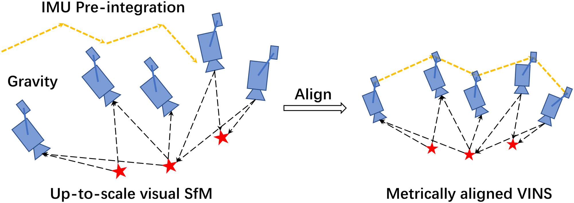
Fig. 4: An illustration of the visual-inertial alignment process for estimator initialization.

图 4：估计器初始化中视觉惯性对齐过程的示意。

V-A Sliding Window Vision-Only SfM

V-A 滑动窗口纯视觉 SfM

The initialization procedure starts with a vision-only SfM to estimate a graph of up-to-scale camera poses and feature positions.

初始化流程从纯视觉 SfM 开始，估计一组仅到尺度的相机位姿和特征位置。

We maintain a sliding window of frames for bounded computational complexity. Firstly, we check feature correspondences between the latest frame and all previous frames. If we can find stable feature tracking (more than 30 tracked features) and sufficient parallax (more than 20 rotation-compensated pixels) between the latest frame and any other frames in the sliding window. we recover the relative rotation and up-to-scale translation between these two frames using the Five-point algorithm [33]. Otherwise, we keep the latest frame in the window and wait for new frames. If the five-point algorithm success, we arbitrarily set the scale and triangulate all features observed in these two frames. Based on these triangulated features, a perspective-n-point (PnP) method [35] is performed to estimate poses of all other frames in the window. Finally, a global full bundle adjustment [36] is applied to minimize the total reprojection error of all feature observations. Since we do not yet have any knowledge about the world frame, we set the first camera frame $(\cdot)^{c_{0}}$ as the reference frame for SfM. All frame poses ($\bar{\mathbf{p}}^{c_{0}}_{c_{k}}$,$\mathbf{q}^{c_{0}}_{c_{k}}$) and feature positions are represented with respect to $(\cdot)^{c_{0}}$. Suppose we have a rough measure extrinsic parameters ($\mathbf{p}^{b}_{c},\mathbf{q}^{b}_{c}$) between the camera and the IMU, we can translate poses from camera frame to body (IMU) frame,

为把计算复杂度限制在有界范围内，我们维持一个滑动窗口的帧。首先，检查最新一帧与所有先前帧之间的特征对应。如果能在最新一帧与滑动窗口中任一其他帧之间找到稳定的特征跟踪（超过 30 个被跟踪特征）以及足够的视差（超过 20 个经旋转补偿的像素），就用五点算法[33]恢复这两帧之间的相对旋转和仅到尺度的平移。否则，把最新一帧留在窗口中，等待新的帧到来。若五点算法成功，我们任意设定尺度，并把这两帧中观测到的所有特征三角化。基于这些已三角化的特征，用透视 n 点（PnP）方法[35]估计窗口中所有其他帧的位姿。最后，做一次全局完整光束法平差[36]，最小化全部特征观测的总重投影误差。由于此时对世界系还一无所知，我们把第一帧相机系 $(\cdot)^{c_{0}}$ 设为 SfM 的参考系。所有帧位姿（$\bar{\mathbf{p}}^{c_{0}}_{c_{k}}$，$\mathbf{q}^{c_{0}}_{c_{k}}$）和特征位置都相对于 $(\cdot)^{c_{0}}$ 表示。假定我们对相机与 IMU 之间的外参（$\mathbf{p}^{b}_{c},\mathbf{q}^{b}_{c}$）已有粗略测量，就可以把位姿从相机系变换到体（IMU）系，

$\begin{split}\mathbf{q}^{c_{0}}_{b_{k}}&=\mathbf{q}^{c_{0}}_{c_{k}}\otimes(\mathbf{q}^{b}_{c})\raisebox{4.95134pt}{\scriptscriptstyle-!1$}\
s\bar{\mathbf{p}}^{c_{0}}{b{k}}&=s\bar{\mathbf{p}}^{c_{0}}{c{k}}-\mathbf{R}^{c_{0}}{b{k}}\mathbf{p}^{b}_{c},\end{split} \tag{14}$$

where $s$ the scaling parameter that aligns the visual structure to the metric scale. Solving this scaling parameter is the key to achieve successful initialization.

其中 $s$ 是把视觉结构对齐到度量尺度的缩放参数。求出这个缩放参数，是成功初始化的关键。

V-B Visual-Inertial Alignment

V-B 视觉惯性对齐

V-B1 Gyroscope Bias Calibration

Consider two consecutive frames $b_{k}$ and $b_{k+1}$ in the window, we get the rotation $\mathbf{q}^{c_{0}}_{b_{k}}$ and $\mathbf{q}^{c_{0}}_{b_{k+1}}$ from the visual SfM, as well as the relative constraint $\hat{\boldsymbol{\gamma}}^{b_{k}}_{b_{k+1}}$ from IMU pre-integration. We linearize the IMU pre-integration term with respect to gyroscope bias and minimize the following cost function:

V-B1 陀螺仪偏置标定

考虑窗口中相邻两帧 $b_{k}$ 和 $b_{k+1}$，我们从视觉 SfM 得到旋转 $\mathbf{q}^{c_{0}}_{b_{k}}$ 和 $\mathbf{q}^{c_{0}}_{b_{k+1}}$，也从 IMU 预积分得到相对约束 $\hat{\boldsymbol{\gamma}}^{b_{k}}_{b_{k+1}}$。我们将 IMU 预积分项对陀螺仪偏置线性化，并最小化如下代价函数：

$\begin{split}\min_{\delta b_{w}}\sum_{k\in\mathcal{B}}\left\|\mathbf{q}^{c_{0}}_{b_{k+1}}\raisebox{4.95134pt}{\scriptscriptstyle-!1$}\otimes\mathbf{q}^{c_{0}}{b{k}}\otimes\boldsymbol{\gamma}^{b_{k}}{b{k+1}}\right|^{2}\
\boldsymbol{\gamma}^{b_{k}}{b{k+1}}\approx\hat{\boldsymbol{\gamma}}^{b_{k}}{b{k+1}}\otimes\begin{bmatrix}1\
\frac{1}{2}\mathbf{J}^{\gamma}{b{w}}\delta\mathbf{b}_{w}\end{bmatrix},\end{split} \tag{15}$$

where $\mathcal{B}$ indexes all frames in the window. We have the first order approximation of $\hat{\boldsymbol{\gamma}}^{b_{k}}_{b_{k+1}}$ with respect to the gyroscope bias using the bias Jacobian derived in Sect. IV-B. In such way, we get an initial calibration of the gyroscope bias $\mathbf{b}_{w}$. Then we re-propagate all IMU pre-integration terms $\hat{\boldsymbol{\alpha}}^{b_{k}}_{b_{k+1}},\hat{\boldsymbol{\beta}}^{b_{k}}_{b_{k+1}}$, and $\hat{\boldsymbol{\gamma}}^{b_{k}}_{b_{k+1}}$ using the new gyroscope bias.

其中 $\mathcal{B}$ 索引窗口中的全部帧。我们利用第 IV-B 节导出的偏置雅可比，得到 $\hat{\boldsymbol{\gamma}}^{b_{k}}_{b_{k+1}}$ 对陀螺仪偏置的一阶近似。这样，我们就得到了陀螺仪偏置 $\mathbf{b}_{w}$ 的初始标定。然后用新的陀螺仪偏置，重新传播所有 IMU 预积分项 $\hat{\boldsymbol{\alpha}}^{b_{k}}_{b_{k+1}},\hat{\boldsymbol{\beta}}^{b_{k}}_{b_{k+1}}$ 和 $\hat{\boldsymbol{\gamma}}^{b_{k}}_{b_{k+1}}$。

V-B2 Velocity, Gravity Vector and Metric Scale Initialization

After the gyroscope bias is initialized, we move on to initialize other essential states for navigation, namely velocity, gravity vector, and metric scale:

V-B2 速度、重力向量与度量尺度初始化

陀螺仪偏置初始化完成后，我们接着初始化导航所需的其他关键状态，即速度、重力向量和度量尺度：

$$\begin{split}\mathcal{X}_{I}&=\left[\mathbf{v}^{b_{0}}_{b_{0}},\,\mathbf{v}^{b_{1}}_{b_{1}},\,\cdots\,\mathbf{v}^{b_{n}}_{b_{n}},\,\mathbf{g}^{c_{0}},\,s\right],\end{split} \tag{16}$$

where $\mathbf{v}^{b_{k}}_{b_{k}}$ is velocity in the body frame while taking the $k^{th}$ image, $\mathbf{g}^{c_{0}}$ is the gravity vector in the $c_{0}$ frame, and $s$ scales the monocular SfM to metric units.

其中 $\mathbf{v}^{b_{k}}_{b_{k}}$ 是拍摄第 $k$ 张图像时体系中的速度，$\mathbf{g}^{c_{0}}$ 是 $c_{0}$ 系中的重力向量，$s$ 把单目 SfM 缩放到度量单位。

Consider two consecutive frames $b_{k}$ and $b_{k+1}$ in the window, then (5) can be written as:

考虑窗口中相邻两帧 $b_{k}$ 和 $b_{k+1}$，则（5）可以写成：

$$\begin{split}{\boldsymbol{\alpha}}^{b_{k}}{b{k+1}}&=\mathbf{R}^{b_{k}}{c{0}}(s(\bar{\mathbf{p}}^{c_{0}}{b{k+1}}-\bar{\mathbf{p}}^{c_{0}}{b{k}})+\frac{1}{2}\mathbf{g}^{c_{0}}{\Delta t}{k}^{2}-\mathbf{R}^{c{0}}{b{k}}\mathbf{v}^{b_{k}}{b{k}}{\Delta t}{k})\
{\boldsymbol{\beta}}^{b{k}}{b{k+1}}&=\mathbf{R}^{b_{k}}{c{0}}(\mathbf{R}^{c_{0}}{b{k+1}}\mathbf{v}^{b_{k+1}}{b{k+1}}+\mathbf{g}^{c_{0}}{\Delta t}{k}-\mathbf{R}^{c{0}}{b{k}}\mathbf{v}^{b_{k}}{b{k}}).\end{split} \tag{17}$$

We can combine (14) and (17) into the following linear measurement model:

我们可以把（14）和（17）组合成如下线性测量模型：

$$\hat{\mathbf{z}}^{b_{k}}{b{k+1}}=\begin{bmatrix}\hat{\boldsymbol{\alpha}}^{b_{k}}{b{k+1}}-\mathbf{p}^{b}{c}+\mathbf{R}^{b{k}}{c{0}}\mathbf{R}^{c_{0}}{b{k+1}}\mathbf{p}^{b}{c}\
\hat{\boldsymbol{\beta}}^{b{k}}{b{k+1}}\end{bmatrix}=\mathbf{H}^{b_{k}}{b{k+1}}\mathcal{X}{I}+\mathbf{n}^{b{k}}{b{k+1}} \tag{18}$$

where,

其中，

$$\mathbf{H}^{b_{k}}{b{k+1}}=\begin{bmatrix}-\mathbf{I}{\Delta t}{k}!&!\mathbf{0}!&!\frac{1}{2}\mathbf{R}^{b{k}}{c{0}}{\Delta t}{k}^{2}!&!\mathbf{R}^{b{k}}{c{0}}(\bar{\mathbf{p}}^{c_{0}}{c{k+1}}-\bar{\mathbf{p}}^{c_{0}}{c{k}})\
-\mathbf{I}!&!\mathbf{R}^{b_{k}}{c{0}}\mathbf{R}^{c_{0}}{b{k+1}}!&!\mathbf{R}^{b_{k}}{c{0}}{\Delta t}_{k}!&!\mathbf{0}\end{bmatrix}! \tag{19}$$

It can be seen that $\mathbf{R}^{c_{0}}_{b_{k}},\mathbf{R}^{c_{0}}_{b_{k+1}},\bar{\mathbf{p}}^{c_{0}}_{c_{k}},\bar{\mathbf{p}}^{c_{0}}_{c_{k+1}}$ are obtained from the up-to-scale monocular visual SfM. ${\Delta t}_{k}$ is the time interval between two consecutive frames. By solving this linear least square problem:

可以看出，$\mathbf{R}^{c_{0}}_{b_{k}},\mathbf{R}^{c_{0}}_{b_{k+1}},\bar{\mathbf{p}}^{c_{0}}_{c_{k}},\bar{\mathbf{p}}^{c_{0}}_{c_{k+1}}$ 来自仅到尺度的单目视觉 SfM。${\Delta t}_{k}$ 是相邻两帧之间的时间间隔。通过求解这个线性最小二乘问题：

$$\begin{split}\min_{\mathcal{X}_{I}}\sum_{k\in\mathcal{B}}\left\|\hat{\mathbf{z}}^{b_{k}}_{b_{k+1}}-\mathbf{H}^{b_{k}}_{b_{k+1}}\mathcal{X}_{I}\right\|^{2},\end{split} \tag{20}$$

we can get body frame velocities for every frame in the window, the gravity vector in the visual reference frame $(\cdot)^{c_{0}}$, as well as the scale parameter.

我们可以得到窗口中每一帧的体系速度、视觉参考系 $(\cdot)^{c_{0}}$ 中的重力向量，以及尺度参数。

V-B3 Gravity Refinement

V-B3 重力精化

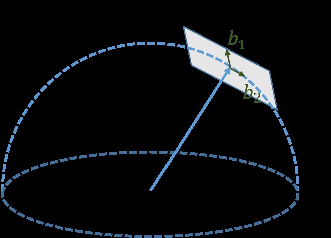
Fig. 5: Illustration of 2 DOF parameterization of gravity. Since the magnitude of gravity is known, $\mathbf{g}$ lies on a sphere with radius $g\approx 9.81m/s^{2}$. The gravity is parameterized around current estimate as $g\cdot\hat{\bar{\mathbf{g}}}+w_{1}\mathbf{b}_{1}+w_{2}\mathbf{b}_{2}$, where $\mathbf{b}_{1}$ and $\mathbf{b}_{2}$ are two orthogonal basis spanning the tangent space.

图 5：重力的二自由度参数化示意。由于重力的大小已知，$\mathbf{g}$ 位于半径为 $g\approx 9.81m/s^{2}$ 的球面上。重力在当前估计附近被参数化为 $g\cdot\hat{\bar{\mathbf{g}}}+w_{1}\mathbf{b}_{1}+w_{2}\mathbf{b}_{2}$，其中 $\mathbf{b}_{1}$ 和 $\mathbf{b}_{2}$ 是张成切空间的一组正交基底。

The gravity vector obtained from the previous linear initialization step can be refined by constraining the magnitude. In most cases, the magnitude of gravity vector is known. This results in only 2 DOF remaining for the gravity vector. We therefore re-parameterize the gravity with two variables on its tangent space. Our parameterization represents the gravity vector as $g\cdot\bar{\hat{\mathbf{g}}}+w_{1}\mathbf{b}_{1}+w_{2}\mathbf{b}_{2}$, where $g$ is the know magnitude of the gravity, $\hat{\bar{\mathbf{g}}}$ is a unit vector representing the gravity direction. $\mathbf{b}_{1}$ and $\mathbf{b}_{2}$ are two orthogonal basis spanning the tangent plane, as shown in Fig. 5. $w_{1}$ and $w_{2}$ are corresponding displacements towards $\mathbf{b}_{1}$ and $\mathbf{b}_{2}$, respectively. We can find one set of $\mathbf{b}_{1}$, $\mathbf{b}_{2}$ by cross products operations using Algorithm 1. Then we substitute $\mathbf{g}$ in (17) by $g\cdot\hat{\bar{\mathbf{g}}}+w_{1}\mathbf{b}_{1}+w_{2}\mathbf{b}_{2}$, and solve for $w_{1}$ and $w_{2}$ together with other state variables. This process iterates until $\hat{\mathbf{g}}$ converges.

前一步线性初始化得到的重力向量，可以通过约束其大小来精化。在多数情况下，重力向量的大小是已知的。这样重力向量就只剩下 2 个自由度。我们因此在其切空间上用两个变量重新参数化重力。我们的参数化把重力向量写成 $g\cdot\bar{\hat{\mathbf{g}}}+w_{1}\mathbf{b}_{1}+w_{2}\mathbf{b}_{2}$，其中 $g$ 是已知的重力大小，$\hat{\bar{\mathbf{g}}}$ 是表示重力方向的单位向量。$\mathbf{b}_{1}$ 和 $\mathbf{b}_{2}$ 是张成切平面的两个正交基底，如图 5 所示。$w_{1}$ 和 $w_{2}$ 分别是沿 $\mathbf{b}_{1}$ 和 $\mathbf{b}_{2}$ 的位移。我们可以用叉乘运算、按算法 1 找到一组 $\mathbf{b}_{1}$、$\mathbf{b}_{2}$。然后把（17）中的 $\mathbf{g}$ 替换为 $g\cdot\hat{\bar{\mathbf{g}}}+w_{1}\mathbf{b}_{1}+w_{2}\mathbf{b}_{2}$，并与其他状态变量一起求解 $w_{1}$ 和 $w_{2}$。这一过程迭代进行，直到 $\hat{\mathbf{g}}$ 收敛。

if $\bar{\hat{\mathbf{g}}}\neq[1,0,0]$ then
$\mathbf{b}_{1}\leftarrow normalize(\bar{\hat{\mathbf{g}}}\times[1,0,0])$;
else
$\mathbf{b}_{1}\leftarrow normalize(\bar{\hat{\mathbf{g}}}\times[0,0,1])$;
end if
$\mathbf{b}_{2}\leftarrow\bar{\hat{\mathbf{g}}}\times\mathbf{b}_{1}$;

Algorithm 1 Finding $\mathbf{b}_{1}$ and $\mathbf{b}_{2}$

if $\bar{\hat{\mathbf{g}}}\neq[1,0,0]$ then
$\mathbf{b}_{1}\leftarrow normalize(\bar{\hat{\mathbf{g}}}\times[1,0,0])$;
else
$\mathbf{b}_{1}\leftarrow normalize(\bar{\hat{\mathbf{g}}}\times[0,0,1])$;
end if
$\mathbf{b}_{2}\leftarrow\bar{\hat{\mathbf{g}}}\times\mathbf{b}_{1}$;

算法 1 求 $\mathbf{b}_{1}$ 和 $\mathbf{b}_{2}$

V-B4 Completing Initialization

After refining the gravity vector, we can get the rotation $\mathbf{q}^{w}_{c_{0}}$ between the world frame and the camera frame $c_{0}$ by rotating the gravity to the z-axis. We then rotate all variables from reference frame $(\cdot)^{c_{0}}$ to the world frame $(\cdot)^{w}$. The body frame velocities will also be rotated to world frame. Translational components from the visual SfM will be scaled to metric units. At this point, the initialization procedure is completed and all these metric values will be fed for a tightly-coupled monocular VIO.

V-B4 完成初始化

精化重力向量之后，我们可以通过把重力转到 $z$ 轴，得到世界系与相机系 $c_{0}$ 之间的旋转 $\mathbf{q}^{w}_{c_{0}}$。然后把所有变量从参考系 $(\cdot)^{c_{0}}$ 转到世界系 $(\cdot)^{w}$。体系速度也将被转到世界系。来自视觉 SfM 的平移分量会被缩放到度量单位。至此，初始化流程完成，这些度量值将被送入紧耦合的单目 VIO。

VI Tightly-coupled Monocular VIO

VI 紧耦合单目 VIO

After estimator initialization, we proceed with a sliding window-based tightly-coupled monocular VIO for high-accuracy and robust state estimation. An illustration of the sliding window formulation is shown in Fig. 3.

估计器初始化之后，我们接着用基于滑动窗口的紧耦合单目 VIO，做高精度、稳健的状态估计。滑动窗口表述的示意见图 3。

VI-A Formulation

VI-A 表述

The full state vector in the sliding window is defined as:

滑动窗口中的完整状态向量定义为：

$$\begin{split}\mathcal{X}&=\left[\mathbf{x}{0},,\mathbf{x}{1},,\cdots,\mathbf{x}{n},,\mathbf{x}^{b}{c},,\lambda_{0},,\lambda_{1},,\cdots,\lambda_{m}\right]\
\mathbf{x}{k}&=\left[\mathbf{p}^{w}{b_{k}},,\mathbf{v}^{w}{b{k}},,\mathbf{q}^{w}{b{k}},,\mathbf{b}{a},,\mathbf{b}{g}\right],k\in[0,n]\
\mathbf{x}^{b}{c}&=\left[\mathbf{p}^{b}{c},,\mathbf{q}^{b}_{c}\right],\end{split} \tag{21}$$

where $\mathbf{x}_{k}$ is the IMU state at the time that the $k^{th}$ image is captured. It contains position, velocity, and orientation of the IMU in the world frame, and acceleration bias and gyroscope bias in the IMU body frame. $n$ is the total number of keyframes, and $m$ is the total number of features in the sliding window. $\lambda_{l}$ is the inverse depth of the $l^{th}$ feature from its first observation.

其中 $\mathbf{x}_{k}$ 是拍摄第 $k$ 张图像时的 IMU 状态。它包含 IMU 在世界系中的位置、速度和姿态，以及 IMU 体系中的加速度计偏置和陀螺仪偏置。$n$ 是关键帧总数，$m$ 是滑动窗口中的特征总数。$\lambda_{l}$ 是第 $l$ 个特征在其首次观测中的逆深度。

We use a visual-inertial bundle adjustment formulation. We minimize the sum of prior and the Mahalanobis norm of all measurement residuals to obtain a maximum posteriori estimation:

我们采用视觉惯性光束法平差的表述。通过最小化先验以及全部测量残差的马氏范数，得到最大后验估计：

$$\displaystyle\min_{\mathcal{X}}\left\{\left\|\mathbf{r}_{p}-\mathbf{H}_{p}\mathcal{X}\right\|^{2}+\sum_{k\in\mathcal{B}}\left\|\mathbf{r}_{\mathcal{B}}(\hat{\mathbf{z}}^{b_{k}}_{b_{k+1}},\,\mathcal{X})\right\|_{\mathbf{P}^{b_{k}}_{b_{k+1}}}^{2}+\right. \\ \displaystyle\left.\sum_{(l,j)\in\mathcal{C}}\rho(\left\|\mathbf{r}_{\mathcal{C}}(\hat{\mathbf{z}}^{c_{j}}_{l},\,\mathcal{X})\right\|_{\mathbf{P}^{c_{j}}_{l}}^{2})\right\},$$

where the Huber norm [37] is defined as:

其中 Huber 范数[37]定义为：

$$\rho(s)=\begin{cases}1&s\geq 1,\
2\sqrt{s}-1&s<1.\end{cases} \tag{23}$$

$\mathbf{r}_{\mathcal{B}}(\hat{\mathbf{z}}^{b_{k}}_{b_{k+1}},\,\mathcal{X})$ and $\mathbf{r}_{\mathcal{C}}(\hat{\mathbf{z}}^{c_{j}}_{l},\,\mathcal{X})$ are residuals for IMU and visual measurements respectively. Detailed definition of the residual terms will be presented in Sect. VI-B and Sect. VI-C. $\mathcal{B}$ is the set of all IMU measurements, $\mathcal{C}$ is the set of features which have been observed at least twice in the current sliding window. $\{\mathbf{r}_{p},\,\mathbf{H}_{p}\}$ is the prior information from marginalization. Ceres Solver [38] is used for solving this nonlinear problem.

$\mathbf{r}_{\mathcal{B}}(\hat{\mathbf{z}}^{b_{k}}_{b_{k+1}},\,\mathcal{X})$ 和 $\mathbf{r}_{\mathcal{C}}(\hat{\mathbf{z}}^{c_{j}}_{l},\,\mathcal{X})$ 分别是 IMU 测量和视觉测量的残差。残差项的详细定义将在第 VI-B 节和第 VI-C 节给出。$\mathcal{B}$ 是全部 IMU 测量的集合，$\mathcal{C}$ 是在当前滑动窗口中至少被观测两次的特征集合。$\{\mathbf{r}_{p},\,\mathbf{H}_{p}\}$ 是来自边缘化的先验信息。该非线性问题用 Ceres Solver[38] 求解。

VI-B IMU Measurement Residual

VI-B IMU 测量残差

Consider the IMU measurements within two consecutive frames $b_{k}$ and $b_{k+1}$ in the sliding window, according to the IMU measurement model defined in (13), the residual for pre-integrated IMU measurement can be defined as:

考虑滑动窗口中相邻两帧 $b_{k}$ 和 $b_{k+1}$ 之间的 IMU 测量，根据（13）中定义的 IMU 测量模型，预积分 IMU 测量的残差可以定义为：

$$\begin{split}&\mathbf{r}{\mathcal{B}}(\hat{\mathbf{z}}^{b{k}}{b{k+1}},,\mathcal{X})=\begin{bmatrix}\delta\boldsymbol{\alpha}^{b_{k}}{b{k+1}}\
\delta\boldsymbol{\beta}^{b_{k}}{b{k+1}}\
\delta\boldsymbol{\theta}^{b_{k}}{b{k+1}}\
\delta{\mathbf{b}{a}}\
\delta{\mathbf{b}{g}}\
\end{bmatrix}\
&=\begin{bmatrix}\mathbf{R}^{b_{k}}{w}(\mathbf{p}^{w}{b_{k+1}}-\mathbf{p}^{w}{b{k}}+\frac{1}{2}\mathbf{g}^{w}\Delta t_{k}^{2}-\mathbf{v}^{w}{b{k}}\Delta t_{k})-\boldsymbol{\hat{\alpha}}^{b_{k}}{b{k+1}}\
\mathbf{R}^{b_{k}}{w}(\mathbf{v}^{w}{b_{k+1}}+\mathbf{g}^{w}\Delta t_{k}-\mathbf{v}^{w}{b{k}})-\boldsymbol{\hat{\beta}}^{b_{k}}{b{k+1}}\
2\begin{bmatrix}\mathbf{q}^{w^{-1}}{b{k}}\otimes\mathbf{q}^{w}{b{k+1}}\otimes(\hat{\boldsymbol{\gamma}}^{b_{k}}{b{k+1}})\raisebox{4.95134pt}{$\scriptscriptstyle-\!1$}\end{bmatrix}{xyz}\
{\mathbf{b}{a}}{b{k+1}}-{\mathbf{b}{a}}{b_{k}}\
{\mathbf{b}{w}}{b_{k+1}}-{\mathbf{b}{w}}{b_{k}}\end{bmatrix},\end{split} \tag{24}$$

where $\begin{bmatrix}\cdot\end{bmatrix}_{xyz}$ extracts the vector part of a quaternion $\mathbf{q}$ for error state representation. $\delta\boldsymbol{\theta}^{b_{k}}_{b_{k+1}}$ is the three dimensional error-state representation of quaternion. [\boldsymbol{\hat{\alpha}}^{b_{k}}_{b_{k+1}},\,\boldsymbol{\hat{\beta}}^{b_{k}}_{b_{k+1}},\,\hat{\boldsymbol{\gamma}}^{b_{k}}_{b_{k+1}}]\mbox{{}^{\text{T}}} are pre-integrated IMU measurement terms using only noisy accelerometer and gyroscope measurements within the time interval between two consecutive image frames. Accelerometer and gyroscope biases are also included in the residual terms for online correction.

其中 $\begin{bmatrix}\cdot\end{bmatrix}_{xyz}$ 取出四元数 $\mathbf{q}$ 的向量部分，用于误差状态表示。$\delta\boldsymbol{\theta}^{b_{k}}_{b_{k+1}}$ 是四元数的三维误差状态表示。[\boldsymbol{\hat{\alpha}}^{b_{k}}{b{k+1}},,\boldsymbol{\hat{\beta}}^{b_{k}}{b{k+1}},,\hat{\boldsymbol{\gamma}}^{b_{k}}{b{k+1}}]\mbox{${}^{\text{T}}$}$ 是仅使用相邻两帧图像时间区间内含噪加速度计和陀螺仪测量得到的预积分 IMU 测量项。加速度计和陀螺仪偏置也被纳入残差项，以便在线校正。

VI-C Visual Measurement Residual

VI-C 视觉测量残差

In contrast to traditional pinhole camera models that define reprojection errors on a generalized image plane, we define the camera measurement residual on a unit sphere. The optics for almost all types of cameras, including wide-angle, fisheye or omnidirectional cameras, can be modeled as a unit ray connecting the surface of a unit sphere. Consider the $l^{th}$ feature that is first observed in the $i^{th}$ image, the residual for the feature observation in the $j^{th}$ image is defined as:

与把重投影误差定义在广义像平面上的传统针孔相机模型不同，我们把相机测量残差定义在单位球上。几乎所有类型相机的光学，包括广角、鱼眼或全向相机，都可以建模为连接单位球面的一条单位射线。考虑第 $l$ 个特征首次在第 $i$ 张图像中被观测到，它在第 $j$ 张图像中的观测残差定义为：

$$\begin{split}&\mathbf{r}{\mathcal{C}}(\hat{\mathbf{z}}^{c{j}}{l},,\mathcal{X})=\begin{bmatrix}\mathbf{b}{1}\ \ \mathbf{b}{2}\end{bmatrix}^{T}\cdot({\hat{\bar{\mathcal{P}}}^{c{j}}{l}}-\frac{\mathcal{P}^{c{j}}{l}}{|\mathcal{P}^{c{j}}{l}|})\
&\hat{\bar{\mathcal{P}}}^{c{j}}{l}=\pi{c}\raisebox{4.95134pt}{$\scriptscriptstyle-\!1$}(\begin{bmatrix}\hat{u}^{c_{j}}{l}\
\hat{v}^{c{j}}{l}\end{bmatrix})\
&\mathcal{P}^{c{j}}{l}=\mathbf{R}^{c}{b}(\mathbf{R}^{b_{j}}{w}(\mathbf{R}^{w}{b_{i}}(\mathbf{R}^{b}{c}\frac{1}{\lambda{l}}\pi_{c}\raisebox{4.95134pt}{$\scriptscriptstyle-\!1$}(\begin{bmatrix}u^{c_{i}}{l}\
v^{c{i}}{l}\end{bmatrix})\
&\qquad\qquad\qquad\qquad\qquad+\mathbf{p}^{b}{c})+\mathbf{p}^{w}{b{i}}-\mathbf{p}^{w}{b{j}})-\mathbf{p}^{b}_{c}),\end{split} \tag{25}$$

where $[u^{c_{i}}_{l},\,v^{c_{i}}_{l}]$ is the first observation of the $l^{th}$ feature that happens in the $i^{th}$ image. $[\hat{u}^{c_{j}}_{l},\,\hat{v}^{c_{j}}_{l}]$ is the observation of the same feature in the $j^{th}$ image. ${\pi}^{-1}_{c}$ is the back projection function which turns a pixel location into a unit vector using camera intrinsic parameters. Since the degrees-of-freedom of the vision residual is two, we project the residual vector onto the tangent plane. $\mathbf{b}_{1},\mathbf{b}_{2}$ are two arbitrarily selected orthogonal bases that span the tangent plane of $\hat{\bar{\mathcal{P}}}^{c_{j}}_{l}$, as shown in Fig. 6. We can find one set of $\mathbf{b}_{1},\mathbf{b}_{2}$ easily, as shown in Algorithm 1. $\mathbf{P}^{c_{j}}_{l}$, as used in (22), is the standard covariance of a fixed length in the tangent space.

其中 $[u^{c_{i}}_{l},\,v^{c_{i}}_{l}]$ 是第 $l$ 个特征在第 $i$ 张图像中的首次观测。[\hat{u}^{c_{j}}{l},,\hat{v}^{c{j}}{l}]$是同一特征在第$j$张图像中的观测。${\pi}^{-1}{c}$是反投影函数，它利用相机内参把像素位置变成单位向量。由于视觉残差的自由度是二，我们把残差向量投影到切平面上。$\mathbf{b}{1},\mathbf{b}{2}$是任意选取的、张成$\hat{\bar{\mathcal{P}}}^{c_{j}}{l}$切平面的两个正交基底，如图 6 所示。我们可以很容易地找到一组$\mathbf{b}{1},\mathbf{b}{2}$，如算法 1 所示。（22）中使用的$\mathbf{P}^{c{j}}_{l}$，是切空间中固定长度的标准协方差。

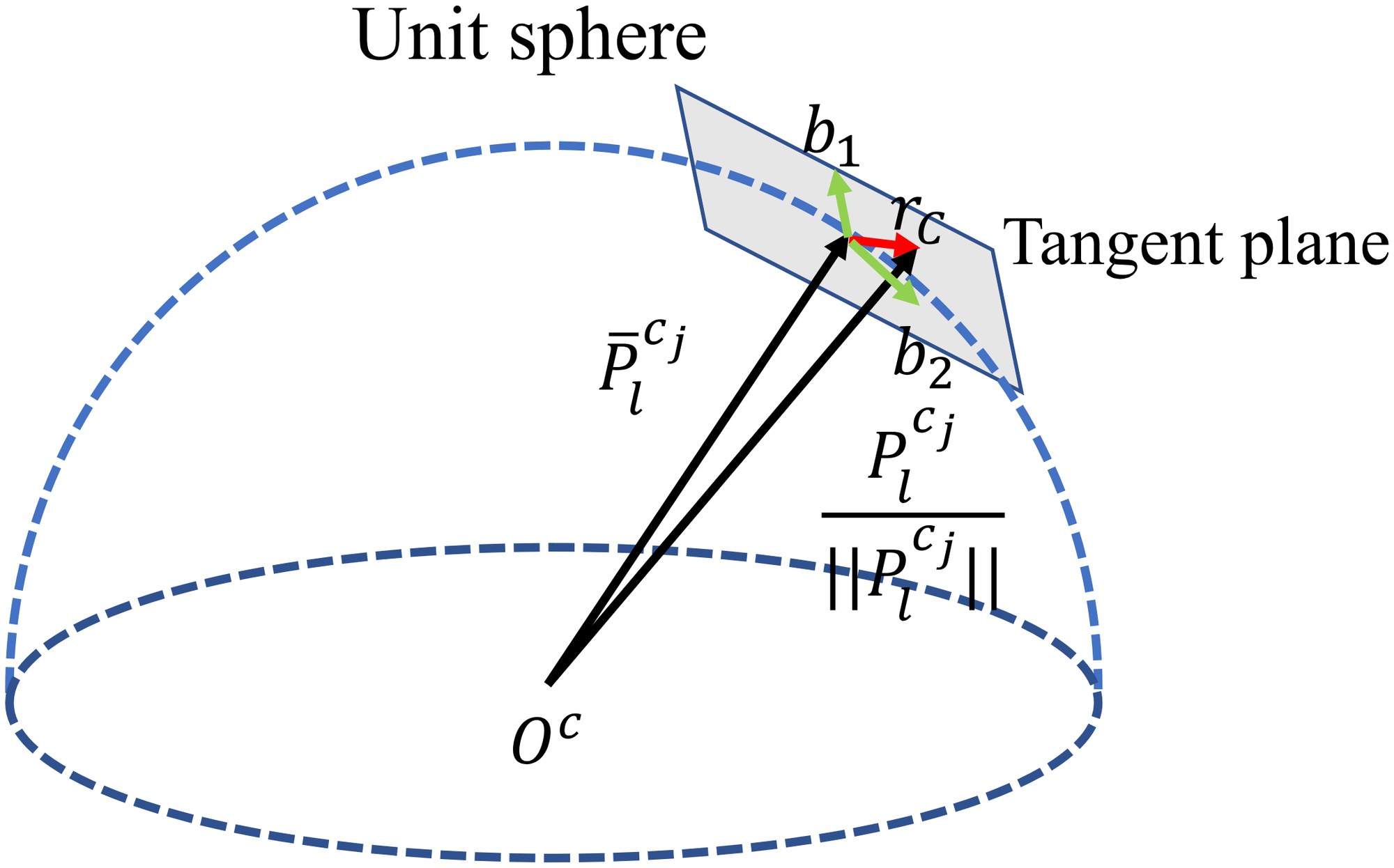
Fig. 6: An illustration of the visual residual on a unit sphere. $\hat{\bar{\mathcal{P}}}^{c_{j}}_{l}$ is the unit vector for the observation of the $l^{th}$ feature in the $j^{th}$ frame. $\mathcal{P}^{c_{j}}_{l}$ is predicted feature measurement on the unit sphere by transforming its first observation in the $i^{th}$ frame to the $j^{th}$ frame. The residual is defined on the tangent plane of $\hat{\bar{\mathcal{P}}}^{c_{j}}_{l}$.

图 6：单位球上视觉残差的示意。$\hat{\bar{\mathcal{P}}}^{c_{j}}_{l}$ 是第 $l$ 个特征在第 $j$ 帧中观测对应的单位向量。$\mathcal{P}^{c_{j}}_{l}$ 是把它在第 $i$ 帧中的首次观测变换到第 $j$ 帧后，在单位球上的预测特征测量。残差定义在 $\hat{\bar{\mathcal{P}}}^{c_{j}}_{l}$ 的切平面上。

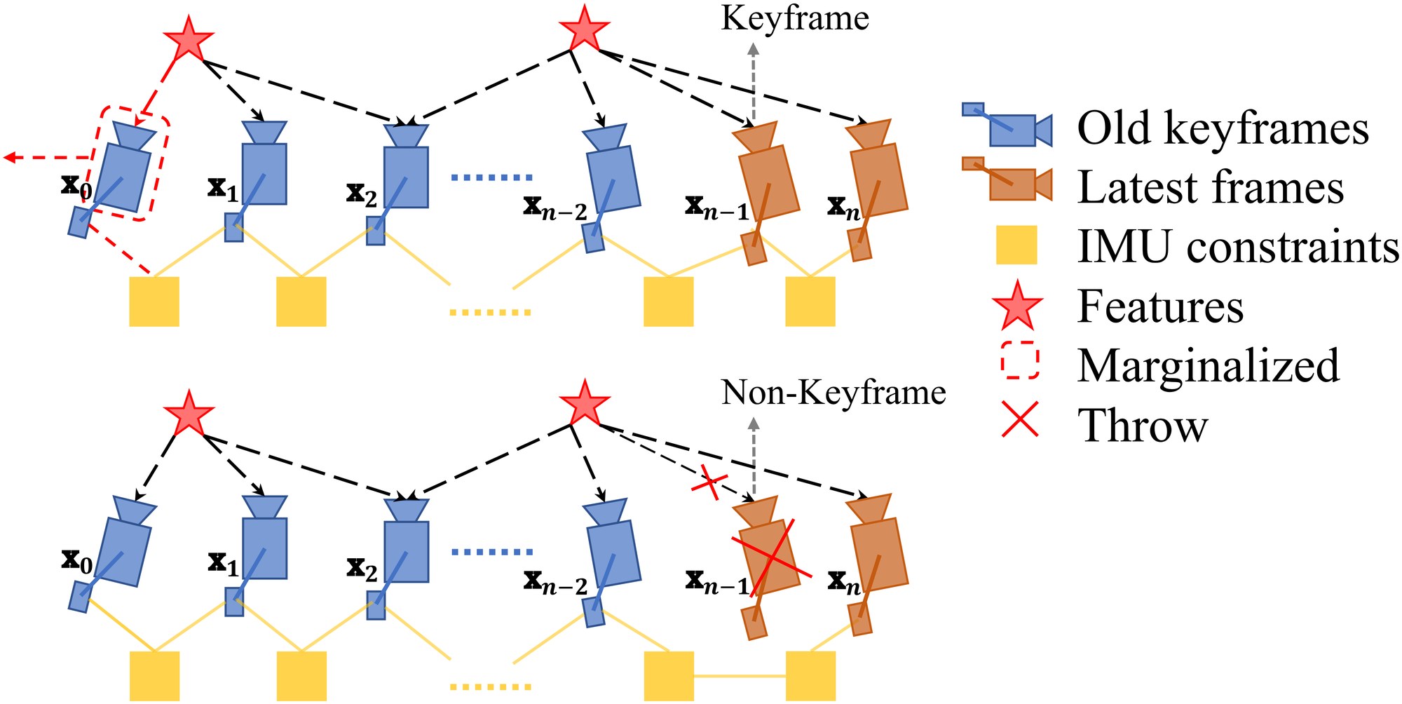
Fig. 7: An illustration of our marginalization strategy. If the second latest frame is a keyframe, we will keep it in the window, and marginalize the oldest frame and its corresponding visual and inertial measurements. Marginalized measurements are turned into a prior. If the second latest frame is not a keyframe, we will simply remove the frame and all its corresponding visual measurements. However, pre-integrated inertial measurements are kept for non-keyframes, and the pre-integration process is continued towards the next frame.

图 7：我们的边缘化策略示意。如果次新帧是关键帧，我们把它留在窗口中，并把最老一帧及其相应的视觉和惯性测量边缘化掉。被边缘化的测量会变成先验。如果次新帧不是关键帧，我们就简单地丢掉该帧及其全部相应的视觉测量。不过，非关键帧的预积分惯性测量会被保留，预积分过程会继续进行到下一帧。

VI-D Marginalization

VI-D 边缘化

In order to bound the computational complexity of our optimization-based VIO, marginalization is incorporated. We selectively marginalize out IMU states $\mathbf{x}_{k}$ and features $\lambda_{l}$ from the sliding window, meanwhile convert measurements corresponding to marginalized states into a prior.

为了把基于优化的 VIO 的计算复杂度限制在有界范围内，我们纳入了边缘化。我们有选择地把 IMU 状态 $\mathbf{x}_{k}$ 和特征 $\lambda_{l}$ 从滑动窗口中边缘化出去，同时把与被边缘化状态相对应的测量转换成先验。

As shown in the Fig. 7, when the second latest frame is a keyframe, it will stay in the window, and the oldest frame is marginalized out with its corresponding measurements. Otherwise, if the second latest frame is a non-keyframe, we throw visual measurements and keep IMU measurements that connect to this non-keyframe. We do not marginalize out all measurements for non-keyframes in order to maintain sparsity of the system. Our marginalization scheme aims to keep spatially separated keyframes in the window. This ensures sufficient parallax for feature triangulation, and maximize the probability of maintaining accelerometer measurements with large excitation.

如图 7 所示，当次新帧是关键帧时，它将留在窗口中，最老一帧连同其相应测量被边缘化掉。反之，如果次新帧是非关键帧，我们就丢掉视觉测量，但保留连接到该非关键帧的 IMU 测量。我们并不把非关键帧的全部测量都边缘化掉，是为了保持系统的稀疏性。我们的边缘化方案旨在让空间上分开的关键帧留在窗口中。这既保证特征三角化有足够的视差，也尽量提高保留具有较大激励的加速度计测量的概率。

The marginalization is carried out using the Schur complement [39]. We construct a new prior based on all marginalized measurements related to the removed state. The new prior is added onto the existing prior.

边缘化用舒尔补[39]完成。我们基于与被移除状态相关的全部被边缘化测量，构造一个新的先验。新先验被加到已有先验上。

We do note that marginalization results in the early fix of linearization points, which may result in suboptimal estimation results. However, since small drifting is acceptable for VIO, we argue that the negative impact caused by marginalization is not critical.

我们也注意到，边缘化会导致线性化点被提前固定，这可能使估计结果不是最优的。不过，由于 VIO 可以接受小的漂移，我们认为边缘化带来的负面影响并不关键。

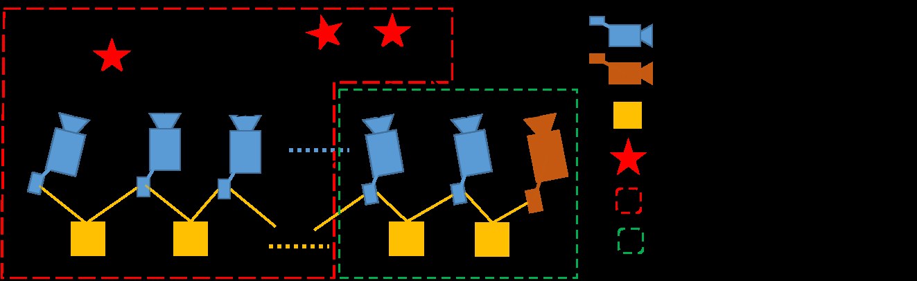
Fig. 8: An illustration of motion-only bundle adjustment for camera-rate outputs.

图 8：用于相机帧率输出的仅运动光束法平差示意。

VI-E Motion-only Visual-Inertial Bundle Adjustment for Camera-Rate State Estimation

VI-E 用于相机帧率状态估计的仅运动视觉惯性光束法平差

For devices with low computational power, such as mobile phones, the tightly-coupled monocular VIO cannot achieve camera-rate outputs due to the heavy computation demands for the nonlinear optimization. To this end, we employ a lightweight motion-only visual-inertial bundle adjustment to boost the state estimation to camera-rate ($~30\,\text{Hz}$).

对计算能力较低的设备，例如手机，紧耦合单目 VIO 由于非线性优化计算量大，无法达到相机帧率的输出。为此，我们采用轻量的仅运动视觉惯性光束法平差，把状态估计提升到相机帧率（约 $30\,\text{Hz}$）。

The cost function for the motion-only visual-inertial bundle adjustment is the same as the one for monocular VIO in (22). However, instead of optimizing all states in the sliding window, we only optimize the poses and velocities of a fixed number of latest IMU states. We treat feature depth, extrinsic parameters, bias, and old IMU states that we do not want to optimize as constant values. We do use all visual and inertial measurements for the motion-only bundle adjustment. This results in much smoother state estimates than single frame PnP methods. An illustration of the proposed strategy is shown in Fig. 8. In contrast to the full tightly-coupled monocular VIO, which may cause more than 50ms on state-of-the-art embedded computers, the motion-only visual-inertial bundle adjustment only takes about 5ms to compute. This enables the low-latency camera-rate pose estimation that is particularly beneficial for drone and AR applications.

仅运动视觉惯性光束法平差的代价函数，与（22）中单目 VIO 的代价函数相同。不过，我们并不优化滑动窗口中的全部状态，而只优化固定数量的最新 IMU 状态的位姿和速度。我们把特征深度、外参、偏置，以及不想优化的旧 IMU 状态当作常量。仅运动光束法平差仍然使用全部视觉和惯性测量。这样得到的状态估计，比单帧 PnP 方法平滑得多。所提策略的示意见图 8。与完整的紧耦合单目 VIO 可能在当时最好的嵌入式计算机上耗时超过 50 毫秒不同，仅运动视觉惯性光束法平差大约只需 5 毫秒。这使得低延迟的相机帧率位姿估计成为可能，对无人机和 AR 应用尤其有益。

VI-F IMU Forward Propagation for IMU-Rate State Estimation

VI-F 用于 IMU 速率状态估计的 IMU 前向传播

IMU measurements come at a much higher rate than visual measurements. Although the frequency of our VIO is limited by image capture frequency, we can still directly propagate the latest VIO estimate with the set of most recent IMU measurements to achieve IMU-rate performance. The high-frequency state estimates can be utilized as state feedback for closed loop closure. An autonomous flight experiment utilizing this IMU-rate state estimates is presented in Sect. IX-D.

IMU 测量的到达速率远高于视觉测量。虽然我们的 VIO 频率受图像采集频率限制，我们仍可以直接用最近一组 IMU 测量，把最新的 VIO 估计向前传播，从而达到 IMU 速率的性能。高频状态估计可以用作闭环控制的状态反馈。利用这种 IMU 速率状态估计的自主飞行实验见第 IX-D 节。

VI-G Failure Detection and Recovery

VI-G 故障检测与恢复

Although our tightly-coupled monocular VIO is robust to various challenging environments and motions. Failure is still unavoidable due to violent illumination change or severely aggressive motions. Active failure detection and recovery strategy can improve the practicability of proposed system. Failure detection is an independent module that detects unusual output from the estimator. We are currently using the following criteria for failure detection:

尽管我们的紧耦合单目 VIO 对各种有挑战的环境和运动都很稳健，但由于剧烈的光照变化或过于猛烈的运动，故障仍不可避免。主动的故障检测与恢复策略可以提高所提系统的实用性。故障检测是一个独立模块，用来发现估计器不寻常的输出。我们目前使用如下准则做故障检测：

• • The number of features being tracking in the latest frame is less than a certain threshold;

• 最新一帧中正在跟踪的特征数量低于某一阈值；

• • Large discontinuity in position or rotation between last two estimator outputs;

• 最近两次估计器输出之间，位置或旋转出现较大间断；

• • Large change in bias or extrinsic parameters estimation;

• 偏置或外参估计发生较大变化；

Once a failure is detected, the system switches back to the initialization phase. Once the monocular VIO is successfully initialized, a new and separate segment of the pose graph will be created.

一旦检测到故障，系统回到初始化阶段。单目 VIO 成功初始化后，将创建一段新的、独立的位姿图分段。

VII Relocalization

VII 重定位

Our sliding window and marginalization scheme bound the computation complexity, but it also introduces accumulated drifts for the system. To be more specific, drifts occur in global 3D position (x, y, z) and the rotation around the gravity direction (yaw). To eliminate drifts, a tightly-coupled relocalization module that seamlessly integrates with the monocular VIO is proposed. The relocalization process starts with a loop detection module that identifies places that have already been visited. Feature-level connections between loop closure candidates and the current frame are then established. These feature correspondences are tightly integrated into the monocular VIO module, resulting in drift-free state estimates with minimum computation overhead. Multiple observations of multiple features are directly used for relocalization, resulting in higher accuracy and better state estimation smoothness. A graphical illustration of the relocalization procedure is shown in Fig. 9(a).

滑动窗口和边缘化方案把计算复杂度限制在有界范围内，但也为系统引入了累积漂移。更具体地说，漂移出现在全局三维位置（x、y、z）以及绕重力方向的旋转（偏航）上。为消除漂移，我们提出一个与单目 VIO 无缝集成的紧耦合重定位模块。重定位过程从回环检测模块开始，识别已经访问过的地点。随后建立回环候选与当前帧之间的特征级连接。这些特征对应被紧耦合地纳入单目 VIO 模块，从而以很小的计算开销得到无漂移的状态估计。多个特征的多次观测被直接用于重定位，因而精度更高、状态估计也更平滑。重定位流程的图示见图 9(a)。

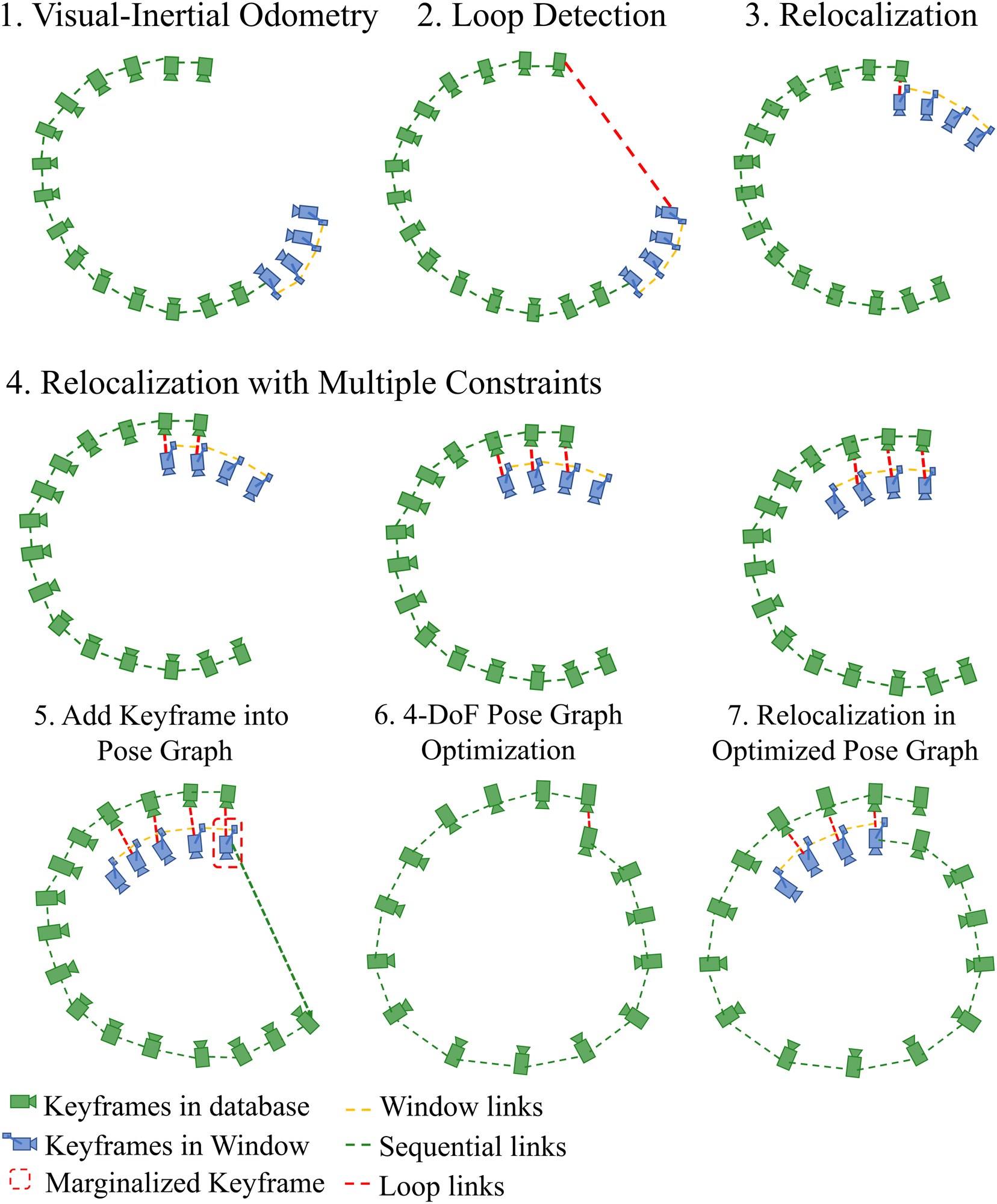
Fig. 9: A diagram illustrating the relocalization and pose graph optimization procedure. Fig. 9(a) shows the relocalization procedure. It starts with VIO-only pose estimates (blue). Past states are recorded (green). If a loop is detected for the newest keyframe (Sect. VII-A), as shown by the red line in the second plot, a relocalization occurred. Note that due to the use of feature-level correspondences for relocalization, we are able to incorporate loop closure constraints from multiple past keyframes (Sect. VII-C), as indicated in the last three plots. The pose graph optimization is illustrated in Fig. 9(b).

(a) Relocalization
(b) Global Pose Graph optimization

图 9：重定位与位姿图优化流程的示意。图 9(a) 展示重定位流程。它从仅含 VIO 的位姿估计（蓝）开始。过去的状态被记录下来（绿）。如果为最新关键帧检测到回环（第 VII-A 节），如第二幅图中红线所示，就会发生一次重定位。需要注意，由于重定位使用特征级对应，我们能够纳入来自多个过去关键帧的回环闭合约束（第 VII-C 节），如最后三幅图所示。位姿图优化见图 9(b)。

(a) 重定位
(b) 全局位姿图优化

VII-A Loop Detection

VII-A 回环检测

We utilize DBoW2 [6], a state-of-the-art bag-of-word place recognition approach, for loop detection. In addition to the corner features that are used for the monocular VIO, 500 more corners are detected and described by the BRIEF descriptor [40]. The additional corner features are used to achieve better recall rate on loop detection. Descriptors are treated as the visual word to query the visual database. DBoW2 returns loop closure candidates after temporal and geometrical consistency check. We keep all BRIEF descriptors for feature retrieving, but discard the raw image to reduce memory consumption.

我们利用当时最好的词袋地点识别方法 DBoW2[6] 做回环检测。除了用于单目 VIO 的角点特征外，再检测 500 个角点，并用 BRIEF 描述子[40] 描述。额外的角点特征用来提高回环检测的召回率。描述子被当作视觉词去查询视觉数据库。DBoW2 在时间和几何一致性检查之后返回回环闭合候选。我们保留全部 BRIEF 描述子用于特征检索，但丢掉原始图像以降低内存消耗。

We note that our monocular VIO is able to render roll and pitch angles observable. As such, we do not need to rely on rotation-invariant features, such as the ORB feature used in ORB SLAM [4].

我们注意到，单目 VIO 已经能够使横滚角和俯仰角可观测。因此，我们不必依赖旋转不变特征，例如 ORB-SLAM[4] 中使用的 ORB 特征。

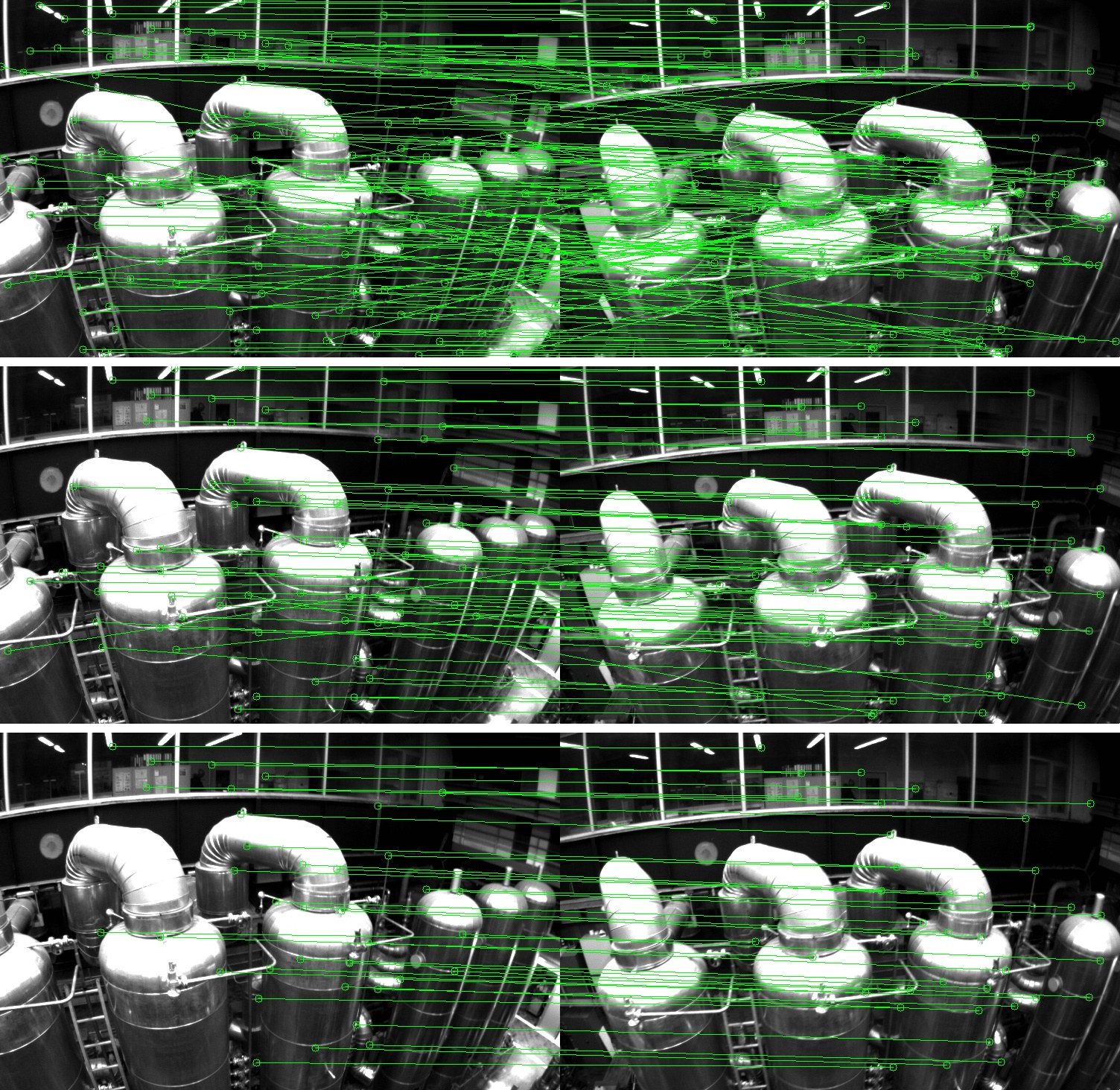
Fig. 10: Descriptor matching and outlier removal for feature retrieval during loop closure.

(a) BRIEF descriptor matching results
(b) First step: 2D-2D outlier rejection results
(c) Second step: 3D-2D outlier rejection results.

图 10：回环闭合期间特征检索的描述子匹配与外点剔除。

(a) BRIEF 描述子匹配结果
(b) 第一步：2D-2D 外点剔除结果
(c) 第二步：3D-2D 外点剔除结果。

VII-B Feature Retrieval

VII-B 特征检索

When a loop is detected, the connection between the local sliding window and the loop closure candidate is established by retrieving feature correspondences. Correspondences are found by BRIEF descriptor matching. Directly descriptor matching may cause a large number a lot of outliers. To this end, we use two-step geometric outlier rejection, as illustrated in Fig. 10.

检测到回环后，通过检索特征对应，建立起局部滑动窗口与回环闭合候选之间的连接。对应由 BRIEF 描述子匹配得到。直接做描述子匹配可能产生大量外点。为此，我们使用两步几何外点剔除，如图 10 所示。

• • 2D-2D: fundamental matrix test with RANSAC [31]. We use 2D observations of retrieved features in the current image and loop closure candidate image to perform fundamental matrix test.

• 2D-2D：带 RANSAC 的基本矩阵检验[31]。我们用当前图像和回环闭合候选图像中被检索特征的二维观测，做基本矩阵检验。

• • 3D-2D: PnP test with RANSAC [35]. Based on the known 3D position of features in the local sliding window, and 2D observations in the loop closure candidate image, we perform PnP test.

• 3D-2D：带 RANSAC 的 PnP 检验[35]。基于局部滑动窗口中特征已知的三维位置，以及回环闭合候选图像中的二维观测，我们做 PnP 检验。

When the number of inliers beyond a certain threshold, we treat this candidate as a correct loop detection and perform relocalization.

当内点数量超过某一阈值时，我们把该候选当作正确的回环检测，并执行重定位。

VII-C Tightly-Coupled Relocalization

VII-C 紧耦合重定位

The relocalization process effectively aligns the current sliding window maintained by the monocular VIO (Sect. VI) to the graph of past poses. During relocalization, we treat poses of all loop closure frames as constants. We jointly optimize the sliding window using all IMU measurements, local visual measurement measurements, and retrieved feature correspondences from loop closure. We can easily write the visual measurement model for retrieved features observed by a loop closure frame $v$ to be the same as those for visual measurements in VIO, as shown in (25). The only difference is that the pose ($\hat{\mathbf{q}}^{w}_{v},\hat{\mathbf{p}}^{w}_{v}$) of the loop closure frame, which is taken from the pose graph (Sect. VIII), or directly from past odometry output (if this is the first relocalization), is treated as a constant. To this end, we can slightly modify the nonlinear cost function in (22) with additional loop terms:

重定位过程有效地把单目 VIO（第 VI 节）所维护的当前滑动窗口，对齐到过去位姿构成的图上。重定位时，我们把所有回环闭合帧的位姿当作常量。我们联合优化滑动窗口，使用全部 IMU 测量、局部视觉测量，以及从回环闭合中检索到的特征对应。我们可以很容易地把回环闭合帧 $v$ 所观测到的检索特征的视觉测量模型，写成与 VIO 中视觉测量相同的形式，如（25）所示。唯一的差别是，取自位姿图（第 VIII 节）、或在第一次重定位时直接取自过去里程计输出的回环闭合帧位姿（$\hat{\mathbf{q}}^{w}_{v},\hat{\mathbf{p}}^{w}_{v}$），被当作常量。为此，我们可以对（22）中的非线性代价函数稍作修改，加入额外的回环项：

$$\displaystyle\min_{\mathcal{X}}\left\{\left\|\mathbf{r}_{p}-\mathbf{H}_{p}\mathcal{X}\right\|^{2}+\sum_{k\in\mathcal{B}}\left\|\mathbf{r}_{\mathcal{B}}(\hat{\mathbf{z}}^{b_{k}}_{b_{k+1}},\mathcal{X})\right\|_{\mathbf{P}^{b_{k}}_{b_{k+1}}}^{2}\right. \\ \displaystyle\left.+\sum_{(l,j)\in\mathcal{C}}\rho(\left\|\mathbf{r}_{\mathcal{C}}(\hat{\mathbf{z}}^{c_{j}}_{l},\mathcal{X})\right\|_{\mathbf{P}^{c_{j}}_{l}}^{2})\right. \\ \displaystyle\left.+\sum_{(l,v)\in\mathcal{L}}\rho(\left\|\mathbf{r}_{\mathcal{C}}(\hat{\mathbf{z}}^{v}_{l},\mathcal{X},\hat{\mathbf{q}}^{w}_{v},\hat{\mathbf{p}}^{w}_{v})\right\|_{\mathbf{P}^{c_{v}}_{l}}^{2}\right\},$$

where $\mathcal{L}$ is the set of the observation of retrieved features in the loop closure frames. ${(l,v)}$ means $l^{th}$ feature observed in the loop closure frame $v$. Note that although the cost function is slightly different from (22), the dimension of the states to be solved remains the same, as poses of loop closure frames are considered as constants. When multiple loop closures are established with the current sliding window, we optimize using all loop closure feature correspondences from all frames at the same time. This gives multi-view constraints for relocalization, resulting in higher accuracy and better smoothness. Note that the global optimization of past poses and loop closure frames happens after relocalization, and will be discussed in Sect. VIII.

其中 $\mathcal{L}$ 是回环闭合帧中对检索特征的观测集合。${(l,v)}$ 表示第 $l$ 个特征在回环闭合帧 $v$ 中被观测到。需要注意，尽管代价函数与（22）略有不同，待求解状态的维数保持不变，因为回环闭合帧的位姿被视为常量。当当前滑动窗口与多个回环同时建立时，我们同时使用来自所有帧的全部回环闭合特征对应进行优化。这为重定位提供了多视角约束，从而得到更高的精度和更好的平滑性。需要说明，过去位姿与回环闭合帧的全局优化发生在重定位之后，将在第 VIII 节讨论。

VIII Global Pose Graph Optimization

VIII 全局位姿图优化

After relocalization, the local sliding window shifts and aligns with past poses. Utilizing the relocalization results, this additional pose graph optimization step is developed to ensure the set of past poses are registered into a globally consistent configuration.

重定位之后，局部滑动窗口发生平移并对齐到过去的位姿。利用重定位结果，这一额外的位姿图优化步骤被用来确保过去的一组位姿登记到全局一致的构型中。

Since our visual-inertial setup renders roll and pitch angles fully observable, the accumulated drift only occurs in four degrees-of-freedom (x, y, z and yaw angle). To this end, we ignore estimating the drift-free roll and pitch states, and only perform 4-DOF pose graph optimization.

由于我们的视觉惯性设置使横滚角和俯仰角完全可观测，累积漂移只发生在四个自由度上（x、y、z 和偏航角）。为此，我们不再估计无漂移的横滚和俯仰状态，而只做 4 自由度位姿图优化。

VIII-A Adding Keyframes into the Pose Graph

VIII-A 把关键帧加入位姿图

When a keyframe is marginalized out from the sliding window, it will be added to pose graph. This keyframe serves as a vertex in the pose graph, and it connects with other vertexes by two types of edges:

当一个关键帧从滑动窗口中被边缘化出去时，它会被加入位姿图。该关键帧作为位姿图中的一个顶点，并通过两类边与其他顶点相连：

VIII-A1 Sequential Edge

a keyframe will establish several sequential edges to its previous keyframes. A sequential edge represents the relative transformation between two keyframes in the local sliding window, which value is taken directly from VIO. Considering a newly marginalized keyframe $i$ and one of its previous keyframes $j$, the sequential edge only contains relative position $\hat{\mathbf{p}}^{i}_{ij}$ and yaw angle $\hat{\psi}_{ij}$.

VIII-A1 顺序边

一个关键帧会与它先前的若干关键帧建立几条顺序边。顺序边表示局部滑动窗口中两个关键帧之间的相对变换，其取值直接来自 VIO。考虑一个新近被边缘化的关键帧 $i$ 及其先前关键帧之一 $j$，顺序边只包含相对位置 $\hat{\mathbf{p}}^{i}_{ij}$ 和偏航角 $\hat{\psi}_{ij}$。

$$\displaystyle\hat{\mathbf{p}}^{i}_{ij}= \\ \displaystyle\hat{\mathbf{R}}^{w}_{i}\raisebox{4.95134pt}{$\scriptscriptstyle-\!1$}(\hat{\mathbf{p}}^{w}_{j}-\hat{\mathbf{p}}^{w}_{i}) \\ \displaystyle\hat{\psi}_{ij}= \\ \displaystyle\hat{{\psi}}_{j}-\hat{\psi}_{i}.$$

VIII-A2 Loop Closure Edge

If the newly marginalized keyframe has a loop connection, it will be connected with the loop closure frame by a loop closure edge in the pose graph. Similarly, the loop closure edge only contains 4-DOF relative pose transform that is defined the same as (27). The value of the loop closure edge is obtained using results from relocalization.

VIII-A2 回环闭合边

如果新近被边缘化的关键帧具有回环连接，它将在位姿图中通过一条回环闭合边与回环闭合帧相连。同样，回环闭合边只包含与（27）定义相同的 4 自由度相对位姿变换。回环闭合边的取值来自重定位的结果。

VIII-B 4-DOF Pose Graph Optimization

VIII-B 四自由度位姿图优化

We define the residual of the edge between frames $i$ and $j$ minimally as:

我们把帧 $i$ 与 $j$ 之间边的残差最小地定义为：

$\begin{split}\mathbf{r}_{i,j}(\mathbf{p}^{w}_{i},\psi_{i},\mathbf{p}^{w}_{j},\psi_{j})=\begin{bmatrix}\mathbf{R}(\hat{\phi}_{i},\hat{\theta}_{i},\psi_{i})\raisebox{4.95134pt}{\scriptscriptstyle-!1$}(\mathbf{p}^{w}{j}-\mathbf{p}^{w}{i})-\hat{\mathbf{p}}^{i}{ij}\
\psi{j}-\psi_{i}-\hat{\psi}_{ij}\
\end{bmatrix}\end{split}, \tag{28}$$

where $\hat{\phi}_{i},\hat{\theta}_{i}$ are the estimates roll and pitch angles, which are obtained directly from monocular VIO.

其中 $\hat{\phi}_{i},\hat{\theta}_{i}$ 是估计得到的横滚角和俯仰角，直接取自单目 VIO。

The whole graph of sequential edges and loop closure edges are optimized by minimizing the following cost function:

由顺序边和回环闭合边组成的整张图，通过最小化如下代价函数来优化：

$$\displaystyle\min_{\mathbf{p},\psi}\left\{\sum_{(i,j)\in\mathcal{S}}\left\|\mathbf{r}_{i,j}\right\|^{2}+\sum_{(i,j)\in\mathcal{L}}\rho(\left\|\mathbf{r}_{i,j}\right\|^{2})\right\},$$

where $\mathcal{S}$ is the set of all sequential edges and $\mathcal{L}$ is the set of all loop closure edges. Although the tightly-coupled relocalization already helps with eliminating wrong loop closures, we add another Huber norm $\rho(\cdot)$ to further reduce the impact of any possible wrong loops. In contrast, we do not use any robust norms for sequential edges, as these edges are extracted from VIO, which already contain sufficient outlier rejection mechanisms.

其中 $\mathcal{S}$ 是全部顺序边的集合，$\mathcal{L}$ 是全部回环闭合边的集合。尽管紧耦合重定位已经有助于剔除错误回环，我们再加一层 Huber 范数 $\rho(\cdot)$，以进一步降低任何可能的错误回环的影响。与此相对，我们对顺序边不使用任何鲁棒范数，因为这些边提取自 VIO，而 VIO 本身已经包含足够的外点剔除机制。

Pose graph optimization and relocalization (Sect. VII-C) runs asynchronously in two separate threads. This enables immediate use of the most optimized pose graph for relocalization whenever it becomes available. Similarly, even if the current pose graph optimization is not completed yet, relocalization can still take place using the existing pose graph configuration. This process is illustrated in Fig.  9(b).

位姿图优化与重定位（第 VII-C 节）在两条独立线程中异步运行。这样，一旦最优化的位姿图可用，就可以立即用于重定位。类似地，即便当前的位姿图优化尚未完成，重定位仍可使用已有的位姿图构型进行。这一过程如图 9(b) 所示。

VIII-C Pose Graph Management

VIII-C 位姿图管理

The size of the pose graph may grow unbounded when the travel distance increases, limiting the real-time performance of the system in the long run. To this end, we implement a downsample process to maintain the pose graph database to a limited size. All keyframes with loop closure constraints will be kept, while other keyframes that are either too close or have very similar orientations to its neighbors may be removed. The probability of a keyframe being removed is proportional to its spatial density to its neighbors.

当行驶距离增加时，位姿图的规模可能无界增长，长期来看会限制系统的实时性能。为此，我们实现了一个下调采样过程，把位姿图数据库维持在有限大小。所有带有回环闭合约束的关键帧都会被保留，而那些与邻居过近、或朝向非常相近的其他关键帧则可能被移除。一个关键帧被移除的概率，与它相对邻居的空间密度成正比。

IX Experimental Results

IX 实验结果

We perform three experiments and two applications to evaluate the proposed VINS-Mono system. In the first experiment, we compare the proposed algorithm with another state-of-the-art algorithm on public datasets. We perform a numerical analysis to show the accuracy of our system. We then test our system in the indoor environment to evaluate the performance in repetitive scenes. A large-scale experiment is carried out to illustrate the long-time practicability of our system. Additionally, we apply the proposed system for two applications. For aerial robot application, we use VINS-Mono for position feedback to control a drone to follow a pre-defined trajectory. We then port our approach onto an iOS mobile device and compare against Google Tango.

我们通过三项实验和两项应用来评估所提出的 VINS-Mono 系统。在第一项实验中，我们在公开数据集上把所提算法与另一种当时最好的算法比较，并用数值分析展示系统精度。随后在室内环境中测试系统，以评估它在重复场景中的表现。还进行了一次大尺度实验，以说明系统在长时间运行中的实用性。此外，我们把所提系统用到两项应用中。在飞行机器人应用中，我们用 VINS-Mono 提供位置反馈，控制无人机沿预定轨迹飞行。随后把方法移植到 iOS 移动设备上，并与 Google Tango 比较。

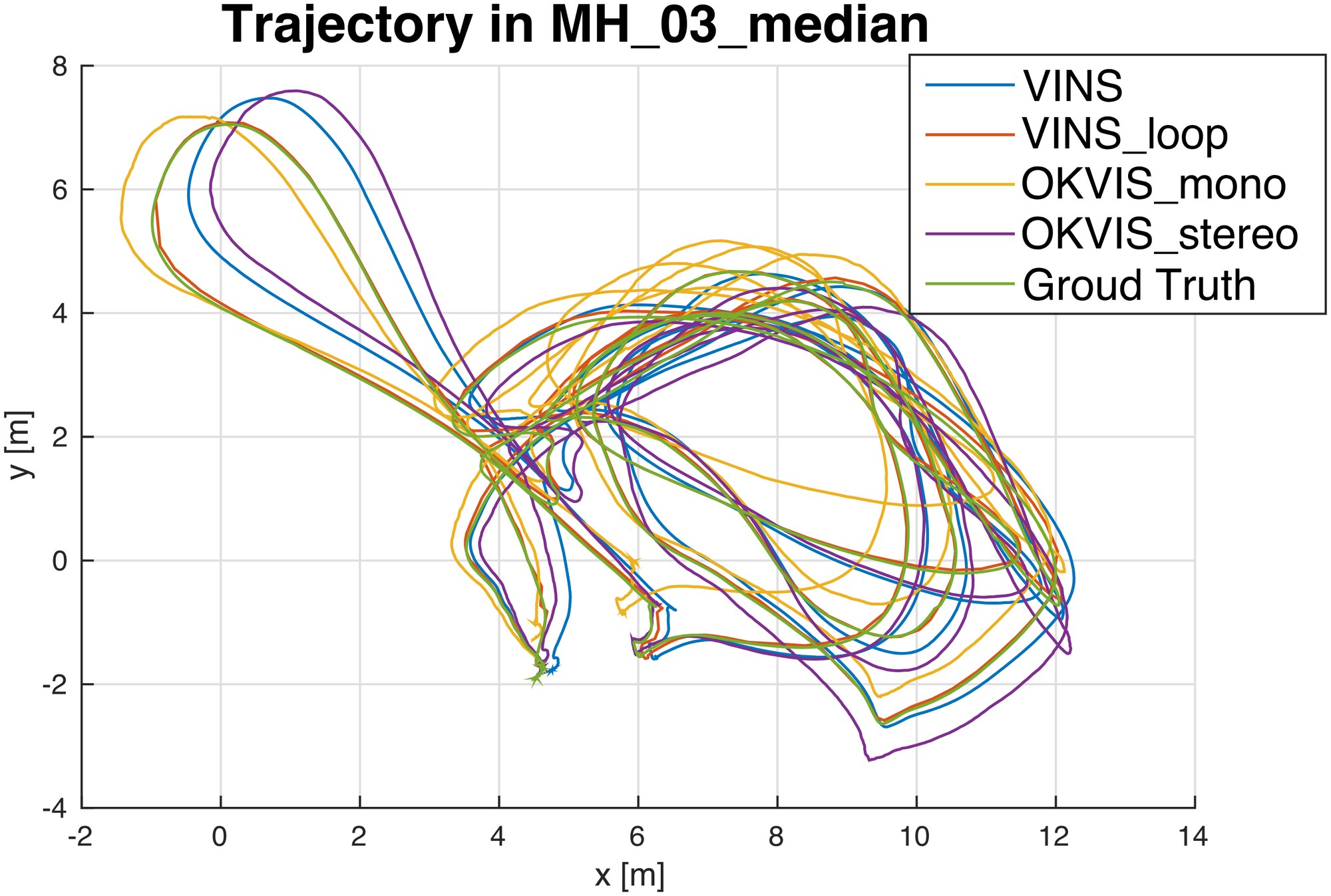
Fig. 11: Trajectory in MH_03_median, compared with OKVIS.

图 11：MH_03_median 中的轨迹，与 OKVIS 比较。

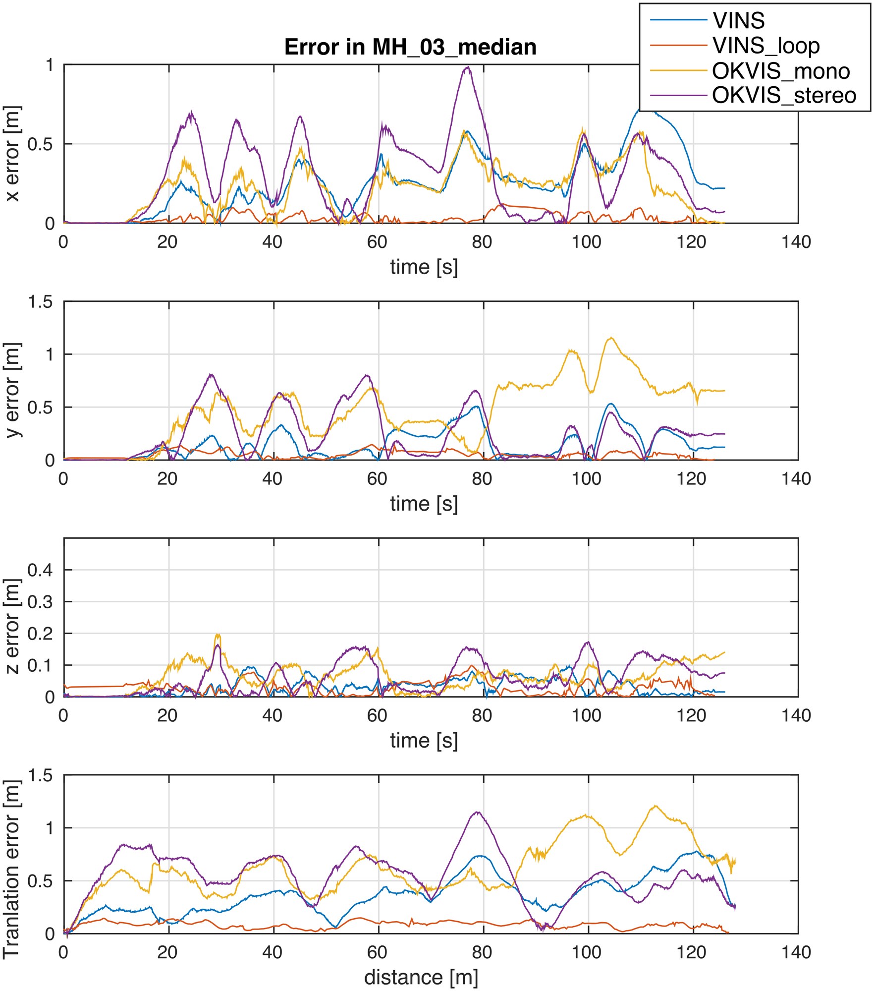
Fig. 12: Translation error plot in MH_03_median.

图 12：MH_03_median 中的平移误差曲线。

IX-A Dataset Comparison

IX-A 数据集比较

We evaluate our proposed VINS-Mono using the EuRoC MAV Visual-Inertial Datasets [41]. The datasets are collected onboard a micro aerial vehicle, which contains stereo images (Aptina MT9V034 global shutter, WVGA monochrome, 20 FPS), synchronized IMU measurements (ADIS16448, 200 Hz), and ground truth states (VICON and Leica MS50). We only use images from the left camera. Large IMU bias and illumination changes are observed in these datasets.

我们用 EuRoC MAV 视觉惯性数据集[41]评估所提出的 VINS-Mono。这些数据集在微型飞行器上采集，包含立体图像（Aptina MT9V034 全局快门，WVGA 单色，20 FPS）、同步 IMU 测量（ADIS16448，200 Hz），以及真值状态（VICON 和 Leica MS50）。我们只使用左目图像。这些数据集中可以观察到较大的 IMU 偏置和光照变化。

In these experiments, we compare VINS-Mono with OKVIS [16], a state-of-the-art VIO that works with monocular and stereo cameras. OKVIS is another optimization-based sliding-window algorithm. Our algorithm is different with OKVIS in many details, as presented in the technical sections. Our system is complete with robust initialization and loop closure. We use two sequences, MH_03_median and MH_05_difficult, to show the performance of proposed method. To simplify the notation, we use VINS to denote our approach with only monocular VIO, and VINS_loop to denote the complete version with relocalization and pose graph optimization. We use OKVIS_mono and OKVIS_stereo to denote the OKVIS’s results using monocular and stereo images respectively. For the fair comparison, we throw the first 100 outputs, and use the following 150 outputs to align with the ground truth, and compare the remaining estimator outputs.

在这些实验中，我们把 VINS-Mono 与 OKVIS[16] 比较，后者是当时最好的、可同时用于单目和双目相机的 VIO。OKVIS 也是一种基于优化的滑动窗口算法。我们的算法在许多细节上与 OKVIS 不同，如技术各节所述。我们的系统是完整的，带有稳健的初始化和回环闭合。我们用 MH_03_median 和 MH_05_difficult 两个序列展示所提方法的表现。为简化记号，我们用 VINS 表示只有单目 VIO 的版本，用 VINS_loop 表示带重定位和位姿图优化的完整版本。我们用 OKVIS_mono 和 OKVIS_stereo 分别表示 OKVIS 使用单目和双目图像的结果。为公平比较，我们丢掉前 100 个输出，用随后 150 个输出与真值对齐，再比较剩余的估计器输出。

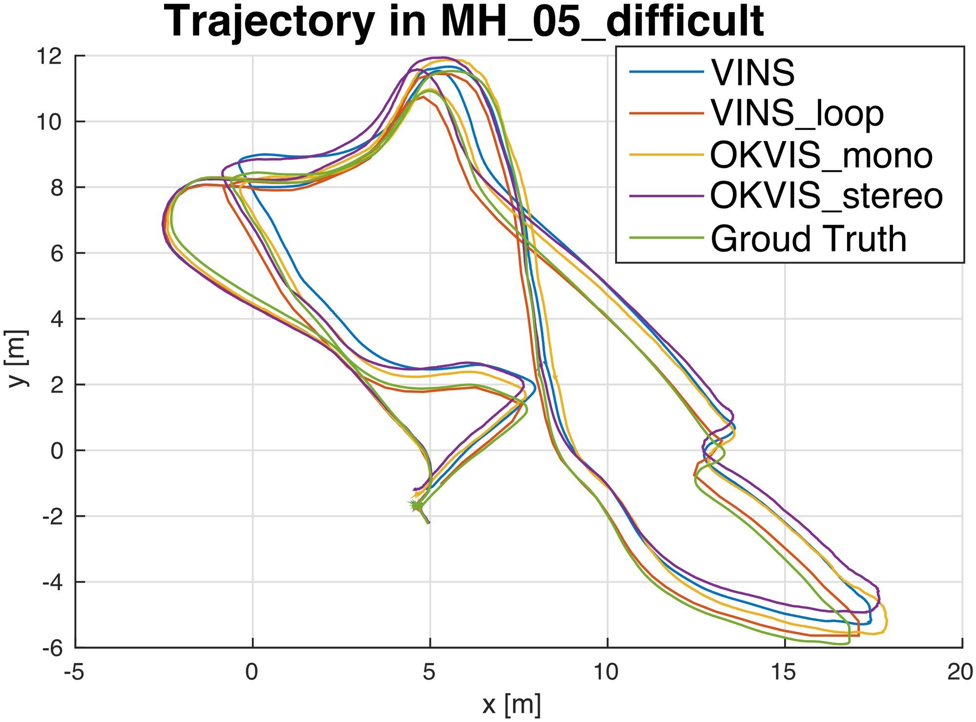
Fig. 13: Trajectory in MH_05_difficult, compared with OKVIS..

图 13：MH_05_difficult 中的轨迹，与 OKVIS 比较。

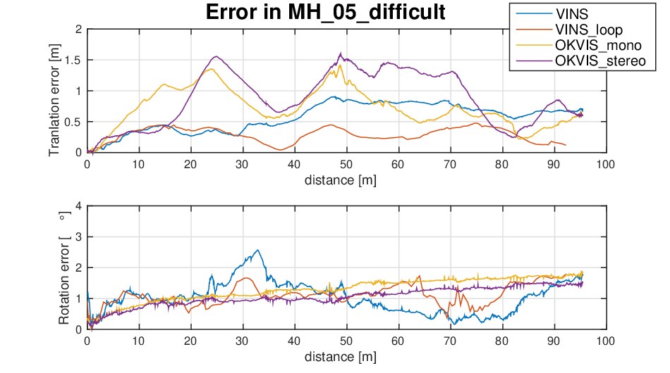
Fig. 14: Translation error and rotation error plot in MH_05_difficult.

图 14：MH_05_difficult 中的平移误差和旋转误差曲线。

For the sequence MH_03_median, the trajectory is shown in Fig. 11. We only compare translation error since rotated motion is negligible in this sequence. The x, y, z error versus time, and the translation error versus distance are shown in Fig. 12. In the error plot, VINS-Mono with loop closure has the smallest translation error. We observe similar results in MH_05_difficult. The proposed method with loop function has the smallest translation error. The translation and rotation errors are shown in Fig. 14. Since the movement is smooth without much yaw angle change in this sequence, only position drift occurs. Obviously, the loop closure capability efficiently bound the accumulated drifts. OKVIS performs better in roll and pitch angle estimation. A possible reason is that VINS-Mono uses the pre-integration technique which is the first-order approximation of IMU propagation to save computation resource.

对序列 MH_03_median，轨迹见图 11。由于该序列中旋转运动可以忽略，我们只比较平移误差。x、y、z 误差随时间的变化，以及平移误差随距离的变化，见图 12。在误差曲线中，带回环闭合的 VINS-Mono 具有最小的平移误差。我们在 MH_05_difficult 中观察到类似结果。带回环功能的所提方法具有最小的平移误差。平移和旋转误差见图 14。由于该序列运动平稳、偏航角变化不大，只出现位置漂移。显然，回环闭合能力有效地约束了累积漂移。OKVIS 在横滚和俯仰角估计上表现更好。一个可能的原因是，VINS-Mono 使用预积分技术，它是 IMU 传播的一阶近似，目的是节省计算资源。

VINS-Mono performs well in all EuRoC datasets, even in the most challenging sequence, V1_03_difficult, the one includes aggressive motion, texture-less area, and significant illumination change. The proposed method can initialize quickly in V1_03_difficult, due to the dedicated initialization procedure.

VINS-Mono 在全部 EuRoC 数据集上都表现良好，即便是最具挑战的序列 V1_03_difficult——其中包含猛烈运动、弱纹理区域和显著的光照变化。由于专门的初始化流程，所提方法可以在 V1_03_difficult 中快速初始化。

For pure VIO, both VINS-Mono and OKVIS have similar accuracy, it is hard to distinguish which one is better. However, VINS-Mono outperforms OKVIS at the system level. It is a complete system with robust initialization and loop closure function to assist the monocular VIO.

就纯 VIO 而言，VINS-Mono 与 OKVIS 具有相近的精度，很难区分哪一个更好。不过，VINS-Mono 在系统层面超过了 OKVIS。它是一套完整系统，带有稳健的初始化和回环闭合功能，来辅助单目 VIO。

IX-B Indoor Experiment

IX-B 室内实验

In the indoor experiment, we choose our laboratory environment as the experiment area. The sensor suite we use is shown in Fig. 15. It contains a monocular camera (20Hz) and an IMU (100Hz) inside the DJI A3 controller[^3]. We hold the sensor suite by hand and walk in normal pace in the laboratory. We encounter pedestrians, low light condition, texture-less area, glass and reflection, as shown in Fig. 16. Videos can be found in the multimedia attachment.

在室内实验中，我们选择实验室环境作为实验区域。所用传感器组合见图 15。它包含一台单目相机（20Hz），以及 DJI A3 飞控内部的 IMU（100Hz）。我们手持传感器组合，在实验室中以正常步速行走。过程中会遇到行人、低光照、弱纹理区域，以及玻璃和反光，如图 16 所示。视频见多媒体附件。

We compare our result with OKVIS, as shown in Fig. 17. Fig. 17(a) is the VIO output from OKVIS. Fig. 17(b) is the VIO-only result from proposed method without loop closure. Fig. 17(c) is the result of the proposed method with relocalization and loop closure. Noticeable VIO drifts occurred when we circle indoor. Both OKVIS and the VIO-only version of VINS-Mono accumulate significant drifts in x, y, z, and yaw angle. Our relocalization and loop closure modules efficiently eliminate all these drifts.

我们把结果与 OKVIS 比较，如图 17 所示。图 17(a) 是 OKVIS 的 VIO 输出。图 17(b) 是所提方法在关闭回环闭合时仅含 VIO 的结果。图 17(c) 是所提方法带重定位和回环闭合的结果。在室内绕圈时出现了明显的 VIO 漂移。OKVIS 和仅含 VIO 的 VINS-Mono 都在 x、y、z 和偏航角上累积了显著漂移。我们的重定位和回环闭合模块有效地消除了这些漂移。

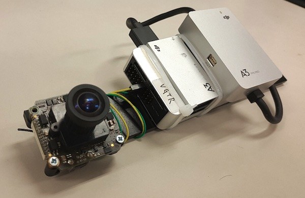
Fig. 15: The device we used for the indoor experiment. It contains one forward-looking global shutter camera (MatrixVision mvBlueFOX-MLC200w) with 752$\times$480 resolution. We use the built-in IMU (ADXL278 and ADXRS290, 100Hz) for the DJI A3 flight controller.

图 15：室内实验所用的装置。它包含一台向前看的全局快门相机（MatrixVision mvBlueFOX-MLC200w），分辨率为 752$\times$480。我们使用 DJI A3 飞控内置的 IMU（ADXL278 和 ADXRS290，100Hz）。

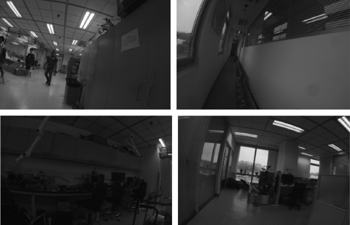
Fig. 16: Sample images for the challenging indoor experiment.

(a) Pedestrians
(b) texture-less area
(c) Low light condition
(d) Glass and reflection

图 16：具有挑战性的室内实验的样本图像。

(a) 行人
(b) 弱纹理区域
(c) 低光照条件
(d) 玻璃与反光

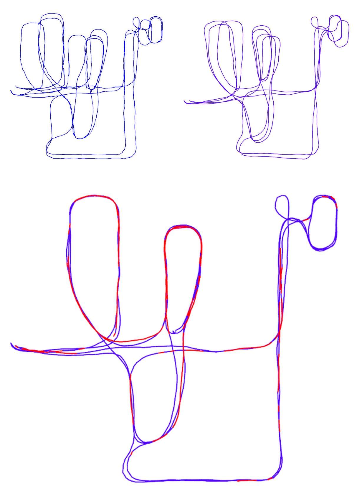
Fig. 17: Results of the indoor experiment with comparison against OKVIS.

(a) Trajectory of OKVIS.
(b) Trajectory of VINS-Mono without loop closure.
(c) Trajectory of VINS-Mono with relocalization and loop closure. Red lines indicate loop detection.

图 17：室内实验结果，并与 OKVIS 比较。

(a) OKVIS 的轨迹。
(b) 关闭回环闭合的 VINS-Mono 轨迹。
(c) 带重定位和回环闭合的 VINS-Mono 轨迹。红线表示回环检测。

IX-C Large-scale Environment

IX-C 大尺度环境

IX-C1 Go out of the lab

We test VINS-Mono in a mixed indoor and outdoor setting. The sensor suite is the same as the one shown in Fig. 15. We started from a seat in the laboratory and go around the indoor space. Then we went down the stairs and walked around the playground outside the building. Next, we went back to the building and go upstairs. Finally, we returned to the same seat in the laboratory. The whole trajectory is more than 700 meters and last approximately ten minutes. A video of the experiment can be found in the multimedia attachment.

IX-C1 走出实验室

我们在室内与室外混合的环境中测试 VINS-Mono。传感器组合与图 15 所示相同。我们从实验室的一个座位出发，先在室内空间绕行，然后下楼，在楼外的运动场周围行走，再回到楼内上楼，最后回到实验室的同一个座位。整段轨迹超过 700 米，大约持续十分钟。实验视频见多媒体附件。

The trajectory is shown in Fig. 19. Fig. 19(a) is the trajectory from OKVIS. When we went up stairs, OKVIS shows unstable feature tracking, resulting in bad estimation. We cannot see the shape of stairs in the red block. The VIO-only result from VINS-Mono is shown in Fig. 19(b). The trajectory with loop closure is shown in Fig. 19(c). The shape of stairs is clear in proposed method. The closed loop trajectory is aligned with Google Map to verify its accuracy, as shown in Fig. 18.

轨迹见图 19。图 19(a) 是 OKVIS 的轨迹。上楼时，OKVIS 出现不稳定的特征跟踪，导致估计变差。我们在红框中看不出楼梯的形状。VINS-Mono 仅含 VIO 的结果见图 19(b)。带回环闭合的轨迹见图 19(c)。所提方法中楼梯的形状是清楚的。闭合后的轨迹与 Google 地图对齐以核对其精度，如图 18 所示。

The final drift for OKVIS is [13.80, -5.26. 7.23]m in x, y and z-axis. The final dirft of VINS-Mono without loop closure is [-5.47, 2.76. -0.29]m, which occupies 0.88% with respect to the total trajectory length, smaller than OKVIS 2.36%. With loop correction. the final drift is bounded to [-0.032, 0.09, -0.07]m, which is trivial compared to the total trajectory length. Although we do not have ground truth, we can still visually inspect that the optimized trajectory is smooth and can be precisely aligned with the satellite map.

OKVIS 的最终漂移在 x、y、z 轴上为 [13.80, -5.26, 7.23] 米。关闭回环闭合的 VINS-Mono 最终漂移为 [-5.47, 2.76, -0.29] 米，占总轨迹长度的 0.88%，小于 OKVIS 的 2.36%。加上回环校正后，最终漂移被约束到 [-0.032, 0.09, -0.07] 米，相对总轨迹长度可以忽略。虽然我们没有真值，仍可以直观看到，优化后的轨迹平滑，并且能够精确地与卫星地图对齐。

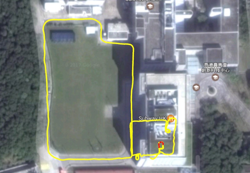
Fig. 18: The estimated trajectory of the mixed indoor and outdoor experiment aligned with Google Map. The yellow line is the final estimated trajectory from VINS-Mono after loop closure. Red lines indicate loop closure.

图 18：室内外混合实验中、与 Google 地图对齐后的估计轨迹。黄线是 VINS-Mono 在回环闭合之后的最终估计轨迹。红线表示回环闭合。

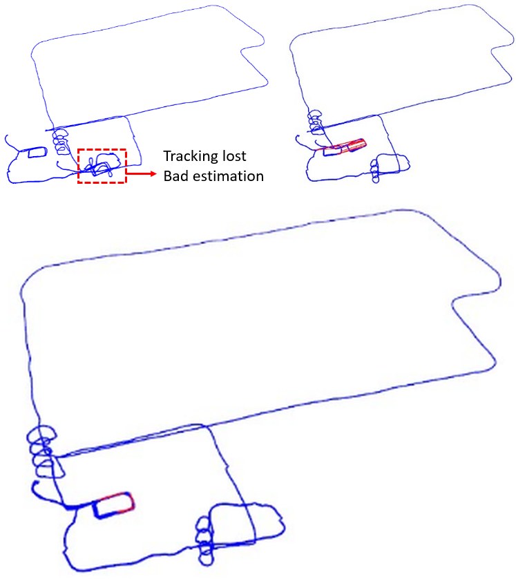
Fig. 19: Estimated trajectories for the mixed indoor and outdoor experiment. In Fig. 19(a), results from OKVIS went bad during tracking lost in texture-less region (staircase). Figs. 19(b) 19(c) shows results from VINS-Mono without and with loop closure. Red lines indicate loop closures. The spiral-shaped blue line shows the trajectory when going up and down the stairs. We can see that VINS-Mono performs well (subject to acceptable drift) even without loop closure.

(a) Estimated trajectory from OKVIS
(b) Estimated trajectory from VINS-Mono with loop closure disabled
(c) Estimated trajectory from VINS-Mono with loop closure

图 19：室内外混合实验的估计轨迹。在图 19(a) 中，OKVIS 的结果在弱纹理区域（楼梯）跟踪丢失时变差。图 19(b)、19(c) 分别是关闭和打开回环闭合的 VINS-Mono 结果。红线表示回环闭合。螺旋状的蓝线是上下楼梯时的轨迹。可以看到，即便关闭回环闭合，VINS-Mono 的表现仍然良好（漂移在可接受范围内）。

(a) OKVIS 的估计轨迹
(b) 关闭回环闭合的 VINS-Mono 估计轨迹
(c) 打开回环闭合的 VINS-Mono 估计轨迹

IX-C2 Go around campus

IX-C2 环绕校园

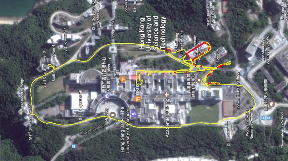
Fig. 20: The estimated trajectory of the very large-scale environment aligned with Google map. The yellow line is the estimated trajectory from VINS-Mono. Red lines indicates loop closure.

图 20：与 Google 地图对齐后的超大尺度环境估计轨迹。黄线是 VINS-Mono 的估计轨迹。红线表示回环闭合。

This very large-scale dataset that goes around the whole HKUST campus was recorded with a handheld VI-Sensor[^4]. The dataset covers the ground that is around 710m in length, 240m in width, and with 60m in height changes. The total path length is 5.62km. The data contains the 25Hz image and 200Hz IMU lasting for 1 hour and 34 minutes. It is a very significant experiment to test the stability and durability of VINS-Mono.

这份环绕整个香港科技大学校园的超大尺度数据，由手持 VI-Sensor 记录。数据覆盖的地面大约长 710 米、宽 240 米，高程变化 60 米。路径总长 5.62 公里。数据包含 25Hz 图像和 200Hz IMU，持续 1 小时 34 分钟。这是检验 VINS-Mono 稳定性和持久性的一次非常重要的实验。

In this large-scale test, We set the keyframe database size to 2000 in order to provide sufficient loop information and achieve real-time performance. We run this dataset with an Intel i7-4790 CPU running at 3.60GHz. Timing statistics are show in Table. I. The estimated trajectory is aligned with Google map in Fig. 20. Compared with Google map, we can see our results are almost drift-free in this very long-duration test.

在这次大尺度测试中，我们把关键帧数据库大小设为 2000，以便提供足够的回环信息，并达到实时性能。我们在一台主频 3.60GHz 的 Intel i7-4790 CPU 上运行这份数据。耗时统计见表 I。估计轨迹与 Google 地图的对齐见图 20。与 Google 地图对照，可以看到在这次很长时长的测试中，我们的结果几乎没有漂移。

Tread	Modules	Time (ms)	Rate (Hz)
1	Feature detector	15	25
KLT tracker	5	25
2	Window optimization	50	10
3	Loop detection	100
Pose graph optimization	130

TABLE I: Timing Statistics

线程	模块	耗时（毫秒）	频率（赫兹）
1	特征检测器	15	25
KLT 跟踪器	5	25
2	窗口优化	50	10
3	回环检测	100
位姿图优化	130

表 I：耗时统计

IX-D Application I: Feedback Control of an Aerial Robot

IX-D 应用一：飞行机器人的反馈控制

We apply VINS-Mono for autonomous feedback control of an aerial robot, as shown in Fig. 21(a). We use a forward-looking global shutter camera (MatrixVision mvBlueFOX-MLC200w) with 752$\times$480 resolution, and equipped it with a 190-degree fisheye lens. A DJI A3 flight controller is used for both IMU measurements and for attitude stabilization control. The onboard computation resource is an Intel i7-5500U CPU running at 3.00 GHz. Traditional pinhole camera model is not suitable for large FOV camera. We use MEI [42] model for this camera, calibrated by the toolkit introduced in [43].

我们把 VINS-Mono 用于飞行机器人的自主反馈控制，如图 21(a) 所示。我们使用一台向前看的全局快门相机（MatrixVision mvBlueFOX-MLC200w），分辨率为 752$\times$480，并配以 190 度鱼眼镜头。一块 DJI A3 飞控既用于 IMU 测量，也用于姿态稳定控制。机载计算资源是一台主频 3.00 GHz 的 Intel i7-5500U CPU。传统针孔相机模型不适合大视场相机。我们为这台相机使用 MEI[42] 模型，并用[43]中介绍的工具包标定。

In this experiment, we test the performance of autonomous trajectory tracking under using state estimates from VINS-Mono. Loop closure is disabled for this experiment The quadrotor is commanded to track a figure eight pattern with each circle being 1.0 meters in radius, as shown in Fig. 21(b). Four obstacles are put around the trajectory to verify the accuracy of VINS-Mono without loop closure. The quadrotor follows this trajectory four times continuously during the experiment. The 100 Hz onboard state estimates (Sect. VI-F) enables real-time feedback control of quadrotor.

在本实验中，我们测试在使用 VINS-Mono 状态估计时的自主轨迹跟踪表现。本实验关闭回环闭合。四旋翼被指令跟踪一个每圈半径 1.0 米的 8 字形轨迹，如图 21(b) 所示。轨迹周围放置了四个已知障碍物，以验证关闭回环闭合时 VINS-Mono 的精度。实验中，四旋翼连续沿该轨迹飞行四次。100 Hz 的机载状态估计（第 VI-F 节）使四旋翼的实时反馈控制成为可能。

Ground truth is obtained using OptiTrack[^5]. Total trajectory length is 61.97 m. The final drift is [0.08, 0.09, 0.13] m, resulting in 0.29% position drift. Details of the translation and rotation as well as their corresponding errors are shown in Fig. 23.

真值由 OptiTrack 获得。轨迹总长 61.97 米。最终漂移为 [0.08, 0.09, 0.13] 米，位置漂移为 0.29%。平移、旋转及其相应误差的细节见图 23。

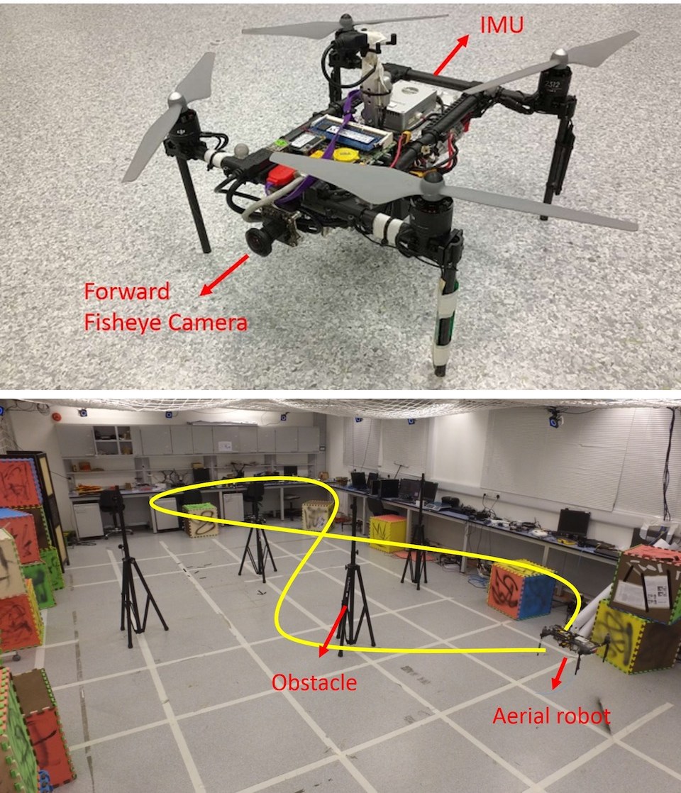
Fig. 21: Fig 21(a): The self-developed aerial robot with a forward-looking fisheye camera (MatrixVision mvBlueFOX-MLC200w, 190 FOV) and an DJI A3 flight controller (ADXL278 and ADXRS290, 100Hz). Fig. 21(b): The designed trajectory. Four known obstacles are placed. The yellow line is the predefined figure eight-figure pattern which the aerial robot should follow. The robot follows the trajectory four times with loop closure disabled. A video of the experiment can be found in the multimedia attachment.

(a) Aerial robot testbed
(b) Testing environment and desired figure eight pattern

图 21：图 21(a)：自行研制的飞行机器人，配有向前看的鱼眼相机（MatrixVision mvBlueFOX-MLC200w，视场 190 度）以及 DJI A3 飞控（ADXL278 和 ADXRS290，100Hz）。图 21(b)：设计轨迹。放置了四个已知障碍物。黄线是飞行机器人应当跟踪的预定 8 字形轨迹。机器人在关闭回环闭合的情况下沿该轨迹飞行四次。实验视频见多媒体附件。

(a) 飞行机器人试验平台
(b) 测试环境与预定的 8 字形轨迹

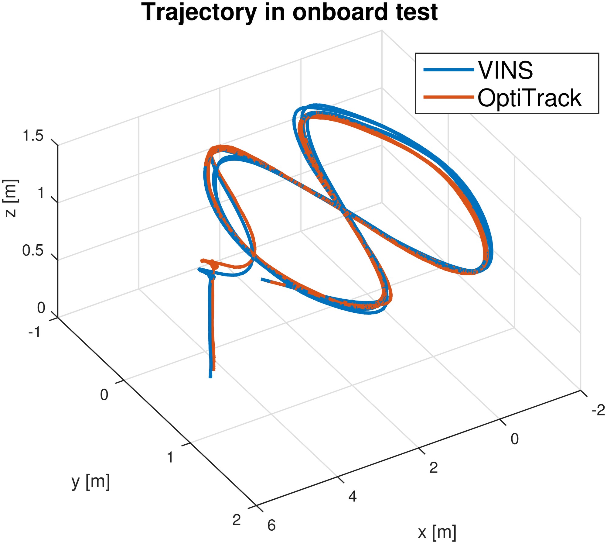
Fig. 22: The trajectory of loop closure-disabled VINS-Mono on the MAV platform and its comparison against the ground truth. The robot follows the trajectory four times. VINS-Mono estimates are used as real-time position feedback for the controller. Ground truth is obtained using OptiTrack. Total length is $61.97m$. Final drift is $0.18m$.

图 22：关闭回环闭合的 VINS-Mono 在微型飞行器平台上的轨迹，及其与真值的比较。机器人沿该轨迹飞行四次。VINS-Mono 的估计被用作控制器的实时位置反馈。真值由 OptiTrack 获得。总长为 $61.97m$。最终漂移为 $0.18m$。

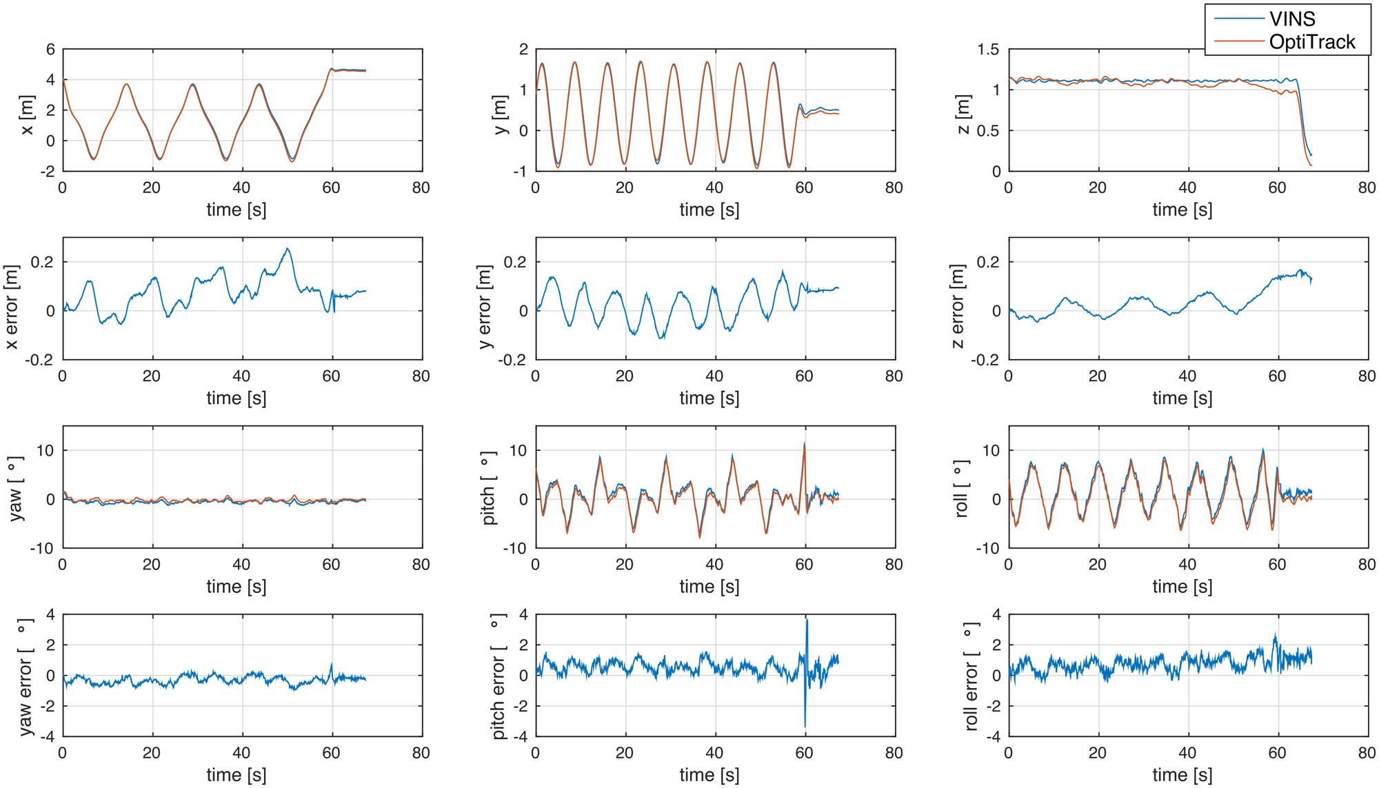
Fig. 23: Position, orientation and their corresponding errors of loop closure-disabled VINS-Mono compared with OptiTrack. A sudden in pitch error at the 60s is caused by aggressive breaking at the end of the designed trajectory, and possible time misalignment error between VINS-Mono and OptiTrack.

图 23：关闭回环闭合的 VINS-Mono 的位置、姿态及其相应误差，并与 OptiTrack 比较。第 60 秒俯仰误差的突然跳变，是由预定轨迹末端的猛烈刹车，以及 VINS-Mono 与 OptiTrack 之间可能的时间对准误差造成的。

IX-E Application II: Mobile Device

IX-E 应用二：移动设备

We port VINS-Mono to mobile devices and present a simple AR application to showcase its accuracy and robustness. We name our mobile implementation VINS-Mobile[^6], and we compare it against Google Tango device[^7], which is one of the best commercially available augmented reality solutions on mobile platforms.

我们把 VINS-Mono 移植到移动设备上，并给出一个简单的 AR 应用，以展示其精度和稳健性。我们把移动端实现命名为 VINS-Mobile，并把它与 Google Tango 设备比较——后者是当时移动平台上最好的商用增强现实方案之一。

VINS-Mono runs on an iPhone7 Plus. we use 30 Hz images with 640 $\times$ 480 resolution captured by the iPhone, and IMU data at 100 Hz obtained by the built-in InvenSense MP67B 6-axis gyroscope and accelerometer. As Fig. 24 shows, we mount the iPhone together with a Tango-Enabled Lenovo Phab 2 Pro. The Tango device uses a global shutter fisheye camera and synchronized IMU for state estimation. Firstly, we insert a virtual cube on the plane which is extracted from estimated visual features as shown in Fig. 25(a). Then we hold these two devices and walk inside and outside the room in a normal pace. When loops are detected, we use the 4-DOF pose graph optimization (Sect. VIII-B) to eliminate x, y, z and yaw drifts.

VINS-Mono 运行在 iPhone 7 Plus 上。我们使用 iPhone 采集的 30 Hz、640 $\times$ 480 分辨率图像，以及由内置 InvenSense MP67B 六轴陀螺仪和加速度计得到的 100 Hz IMU 数据。如图 24 所示，我们把 iPhone 与一台支持 Tango 的联想 Phab 2 Pro 固定在一起。Tango 设备使用全局快门鱼眼相机和同步 IMU 做状态估计。首先，我们在从图估计的视觉特征中提取出的平面上放入一个虚拟立方体，如图 25(a) 所示。然后手持这两台设备，以正常步速在房间内外行走。检测到回环时，我们用四自由度位姿图优化（第 VIII-B 节）消除 x、y、z 和偏航漂移。

Interestingly, when we open a door, Tango’s yaw estimation jumps a big angle, as shown in Fig. 25(b). The reason maybe estimator crash caused by unstable feature tracking or active failure detection and recovery. However, VINS-Mono still works well in this challenging case. After traveling about 264m, we return to the start location. The final result can be seen in Fig. 25(c), the trajectory of Tango suffers drifting in the last lap while our VINS returns to the start point. The drift in total trajectory is eliminated due to the 4-DOF pose graph optimization. This is also evidenced by the fact that the cube is registered to the same place on the image comparing to the beginning.

有意思的是，当我们打开一扇门时，Tango 的偏航估计跳过了一个很大的角度，如图 25(b) 所示。原因可能是特征跟踪不稳定导致的估计器崩溃，或主动故障检测与恢复。然而，在这种有挑战的情形下，VINS-Mono 仍然工作良好。行驶约 264 米后，我们回到起点。最终结果见图 25(c)：Tango 的轨迹在最后一圈出现了漂移，而我们的 VINS 回到了起点。整段轨迹中的漂移由于四自由度位姿图优化而被消除。虚拟立方体在图像中仍然配准到与开始时相同的位置，也说明了这一点。

Admittedly, Tango is more accurate than our implementation especially for local state estimates. However, this experiment shows that the proposed method can run on general mobile devices and have the potential ability to compare specially engineered devices. The robustness of proposed method is also proved in this experiment. Video can be found in the multimedia attachment.

应当承认，尤其在局部状态估计上，Tango 比我们的实现更准确。不过，本实验表明所提方法可以运行在通用移动设备上，并有潜力与专门设计的设备相比较。所提方法的稳健性也在本实验中得到了证明。视频见多媒体附件。

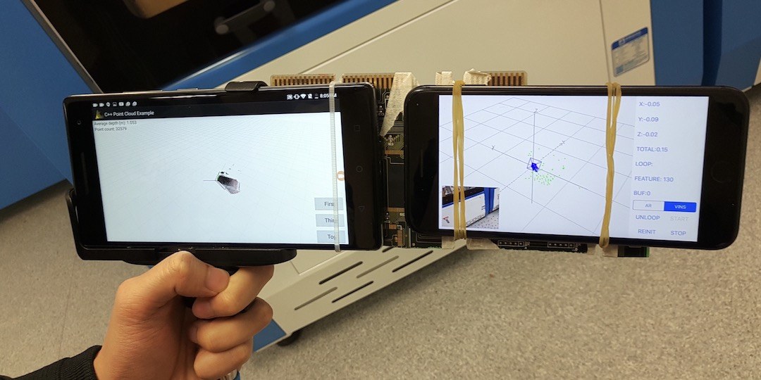
Fig. 24: A simple holder that we used to mount the Google Tango device (left) and the iPhone7 Plus (right) that runs our VINS-Mobile implementation.

图 24：我们用来同时固定 Google Tango 设备（左）和运行 VINS-Mobile 实现的 iPhone 7 Plus（右）的一个简单支架。

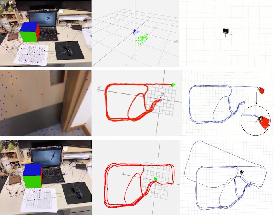
Fig. 25: From left to right: AR image from VINS-Mobile, estimated trajectory from VINS-Mono, estimated trajectory from Tango. Fig. 25(a): Both VINS-Mobile and Tango are initialized at the start location and a virtual box is inserted on the plane which extracted from estimated features. Fig. 25(b): A challenging case in which the camera is facing a moving door. The drift of Tango trajectory is highlighted. Fig. 25(c): The final trajectory of both VINS-Mobile and Tango. The total length is about 264m.

(a) Beginning
(b) Door opening
(c) End

图 25：从左到右：来自 VINS-Mobile 的 AR 图像、VINS-Mono 的估计轨迹、Tango 的估计轨迹。图 25(a)：VINS-Mobile 与 Tango 都在起点初始化，并在从估计特征中提取出的平面上放入一个虚拟方盒。图 25(b)：相机对着一扇正在移动的门，这是一个有挑战的情形。Tango 轨迹的漂移被标出。图 25(c)：VINS-Mobile 与 Tango 的最终轨迹。总长约 264 米。

(a) 开始
(b) 开门
(c) 结束

X Conclusion and Future Work

X 结论与后续工作

In this paper, we propose a robust and versatile monocular visual-inertial estimator. Our approach features both state-of-the-art and novel solutions to IMU pre-integration, estimator initialization and failure recovery, online extrinsic calibration, tightly-coupled visual-inertial odometry, relocalization, and efficient global optimization. We show superior performance by comparing against both state-of-the-art open source implementations and highly optimized industry solutions. We open source both PC and iOS implementation for the benefit of the community.

本文提出一种稳健而通用的单目视觉惯性估计器。我们的方法在 IMU 预积分、估计器初始化与故障恢复、在线外参标定、紧耦合视觉惯性里程计、重定位以及高效全局优化上，既包含当时最好的方案，也包含新的解决方案。通过与当时最好的开源实现以及高度优化的工业方案比较，我们展示了更优的表现。为了回馈社区，我们开源了电脑端和 iOS 端的实现。

Although feature-based VINS estimators have already reached the maturity of real-world deployment, we still see many directions for future research. Monocular VINS may reach weakly observable or even degenerate conditions depending on the motion and the environment. We are most interested in online methods to evaluate the observability properties of monocular VINS, and online generation of motion plans to restore observability. Another research direction concerns the mass deployment of monocular VINS on a large variety of consumer devices, such as mobile phones. This application requires online calibration of almost all sensor intrinsic and extrinsic parameters, as well as the online identification of calibration qualities. Finally, we are interested in producing dense maps given results from monocular VINS. Our first results on monocular visual-inertial dense mapping with application to drone navigation was presented in [44]. However, extensive research is still necessary to further improve the system accuracy and robustness.

尽管基于特征的 VINS 估计器已经达到可以真实部署的成熟程度，我们仍然看到许多后续研究方向。单目 VINS 可能因运动和环境而进入弱可观测、甚至退化的条件。我们最感兴趣的，是在线评估单目 VINS 可观测性的方法，以及在线生成运动规划以恢复可观测性。另一个研究方向，关系到把单目 VINS 大规模部署到手机等各类消费设备上。这类应用几乎需要对全部传感器内参和外参做在线标定，并在线识别标定质量。最后，我们感兴趣的是，在单目 VINS 的结果之上生成稠密地图。我们关于单目视觉惯性稠密建图及其在无人机导航中应用的第一批结果已在[44]中给出。不过，要进一步提高系统精度和稳健性，仍需要大量研究。

References

参考文献

[1] G. Klein and D. Murray, “Parallel tracking and mapping for small ar workspaces,” in Mixed and Augmented Reality, 2007. ISMAR 2007. 6th IEEE and ACM International Symposium on . IEEE, 2007, pp. 225–234.

[2] C. Forster, M. Pizzoli, and D. Scaramuzza, “SVO: Fast semi-direct monocular visual odometry,” in Proc. of the IEEE Int. Conf. on Robot. and Autom. , Hong Kong, China, May 2014.

[3] J. Engel, T. Schöps, and D. Cremers, “Lsd-slam: Large-scale direct monocular slam,” in European Conference on Computer Vision . Springer International Publishing, 2014, pp. 834–849.

[4] R. Mur-Artal, J. Montiel, and J. D. Tardos, “Orb-slam: a versatile and accurate monocular slam system,” IEEE Transactions on Robotics , vol. 31, no. 5, pp. 1147–1163, 2015.

[5] J. Engel, V. Koltun, and D. Cremers, “Direct sparse odometry,” IEEE Transactions on Pattern Analysis and Machine Intelligence , 2017.

[6] D. Gálvez-López and J. D. Tardós, “Bags of binary words for fast place recognition in image sequences,” IEEE Transactions on Robotics , vol. 28, no. 5, pp. 1188–1197, October 2012.

[7] S. Shen, N. Michael, and V. Kumar, “Tightly-coupled monocular visual-inertial fusion for autonomous flight of rotorcraft MAVs,” in Proc. of the IEEE Int. Conf. on Robot. and Autom. , Seattle, WA, May 2015.

[8] Z. Yang and S. Shen, “Monocular visual–inertial state estimation with online initialization and camera–imu extrinsic calibration,” IEEE Transactions on Automation Science and Engineering , vol. 14, no. 1, pp. 39–51, 2017.

[9] T. Qin and S. Shen, “Robust initialization of monocular visual-inertial estimation on aerial robots.” in Proc. of the IEEE/RSJ Int. Conf. on Intell. Robots and Syst. , Vancouver, Canada, 2017, accepted.

[10] P. Li, T. Qin, B. Hu, F. Zhu, and S. Shen, “Monocular visual-inertial state estimation for mobile augmented reality.” in Proc. of the IEEE Int. Sym. on Mixed adn Augmented Reality , Nantes, France, 2017, accepted.

[11] S. Weiss, M. W. Achtelik, S. Lynen, M. Chli, and R. Siegwart, “Real-time onboard visual-inertial state estimation and self-calibration of mavs in unknown environments,” in Robotics and Automation (ICRA), 2012 IEEE International Conference on . IEEE, 2012, pp. 957–964.

[12] S. Lynen, M. W. Achtelik, S. Weiss, M. Chli, and R. Siegwart, “A robust and modular multi-sensor fusion approach applied to mav navigation,” in Proc. of the IEEE/RSJ Int. Conf. on Intell. Robots and Syst.  IEEE, 2013, pp. 3923–3929.

[13] A. I. Mourikis and S. I. Roumeliotis, “A multi-state constraint Kalman filter for vision-aided inertial navigation,” in Proc. of the IEEE Int. Conf. on Robot. and Autom. , Roma, Italy, Apr. 2007, pp. 3565–3572.

[14] M. Li and A. Mourikis, “High-precision, consistent EKF-based visual-inertial odometry,” Int. J. Robot. Research , vol. 32, no. 6, pp. 690–711, May 2013.

[15] M. Bloesch, S. Omari, M. Hutter, and R. Siegwart, “Robust visual inertial odometry using a direct ekf-based approach,” in Proc. of the IEEE/RSJ Int. Conf. on Intell. Robots and Syst.  IEEE, 2015, pp. 298–304.

[16] S. Leutenegger, S. Lynen, M. Bosse, R. Siegwart, and P. Furgale, “Keyframe-based visual-inertial odometry using nonlinear optimization,” Int. J. Robot. Research , vol. 34, no. 3, pp. 314–334, Mar. 2014.

[17] R. Mur-Artal and J. D. Tardos, “Visual-inertial monocular SLAM with map reuse,” arXiv preprint arXiv:1610.05949 , 2016.

[18] K. Wu, A. Ahmed, G. A. Georgiou, and S. I. Roumeliotis, “A square root inverse filter for efficient vision-aided inertial navigation on mobile devices.” in Robotics: Science and Systems , 2015.

[19] M. K. Paul, K. Wu, J. A. Hesch, E. D. Nerurkar, and S. I. Roumeliotis, “A comparative analysis of tightly-coupled monocular, binocular, and stereo vins,” in Proc. of the IEEE Int. Conf. on Robot. and Autom. , Singapore, May 2017.

[20] M. Kaess, H. Johannsson, R. Roberts, V. Ila, J. J. Leonard, and F. Dellaert, “isam2: Incremental smoothing and mapping using the bayes tree,” The International Journal of Robotics Research , vol. 31, no. 2, pp. 216–235, 2012.

[21] V. Usenko, J. Engel, J. Stückler, and D. Cremers, “Direct visual-inertial odometry with stereo cameras,” in Proc. of the IEEE Int. Conf. on Robot. and Autom.  IEEE, 2016, pp. 1885–1892.

[22] T. Lupton and S. Sukkarieh, “Visual-inertial-aided navigation for high-dynamic motion in built environments without initial conditions,” IEEE Trans. Robot. , vol. 28, no. 1, pp. 61–76, Feb. 2012.

[23] C. Forster, L. Carlone, F. Dellaert, and D. Scaramuzza, “IMU preintegration on manifold for efficient visual-inertial maximum-a-posteriori estimation,” in Proc. of Robot.: Sci. and Syst. , Rome, Italy, Jul. 2015.

[24] S. Shen, Y. Mulgaonkar, N. Michael, and V. Kumar, “Initialization-free monocular visual-inertial estimation with application to autonomous MAVs,” in Proc. of the Int. Sym. on Exp. Robot. , Marrakech, Morocco, Jun. 2014.

[25] A. Martinelli, “Closed-form solution of visual-inertial structure from motion,” Int. J. Comput. Vis. , vol. 106, no. 2, pp. 138–152, 2014.

[26] J. Kaiser, A. Martinelli, F. Fontana, and D. Scaramuzza, “Simultaneous state initialization and gyroscope bias calibration in visual inertial aided navigation,” IEEE Robotics and Automation Letters , vol. 2, no. 1, pp. 18–25, 2017.

[27] M. Faessler, F. Fontana, C. Forster, and D. Scaramuzza, “Automatic re-initialization and failure recovery for aggressive flight with a monocular vision-based quadrotor,” in Proc. of the IEEE Int. Conf. on Robot. and Autom.  IEEE, 2015, pp. 1722–1729.

[28] H. Strasdat, J. Montiel, and A. J. Davison, “Scale drift-aware large scale monocular slam,” Robotics: Science and Systems VI , 2010.

[29] B. D. Lucas and T. Kanade, “An iterative image registration technique with an application to stereo vision,” in Proc. of the Intl. Joint Conf. on Artificial Intelligence , Vancouver, Canada, Aug. 1981, pp. 24–28.

[30] J. Shi and C. Tomasi, “Good features to track,” in Computer Vision and Pattern Recognition, 1994. Proceedings CVPR’94., 1994 IEEE Computer Society Conference on . IEEE, 1994, pp. 593–600.

[31] R. Hartley and A. Zisserman, Multiple view geometry in computer vision . Cambridge university press, 2003.

[32] A. Heyden and M. Pollefeys, “Multiple view geometry,” Emerging Topics in Computer Vision , 2005.

[33] D. Nistér, “An efficient solution to the five-point relative pose problem,” IEEE transactions on pattern analysis and machine intelligence , vol. 26, no. 6, pp. 756–770, 2004.

[34] T. Liu and S. Shen, “Spline-based initialization of monocular visual-inertial state estimators at high altitude,” IEEE Robotics and Automation Letters , 2017, accepted.

[35] V. Lepetit, F. Moreno-Noguer, and P. Fua, “Epnp: An accurate o (n) solution to the pnp problem,” International journal of computer vision , vol. 81, no. 2, pp. 155–166, 2009.

[36] B. Triggs, P. F. McLauchlan, R. I. Hartley, and A. W. Fitzgibbon, “Bundle adjustment—a modern synthesis,” in International workshop on vision algorithms . Springer, 1999, pp. 298–372.

[37] P. Huber, “Robust estimation of a location parameter,” Annals of Mathematical Statistics , vol. 35, no. 2, pp. 73–101, 1964.

[38] S. Agarwal, K. Mierle, and Others, “Ceres solver,” http://ceres-solver.org .

[39] G. Sibley, L. Matthies, and G. Sukhatme, “Sliding window filter with application to planetary landing,” J. Field Robot. , vol. 27, no. 5, pp. 587–608, Sep. 2010.

[40] M. Calonder, V. Lepetit, C. Strecha, and P. Fua, “Brief: Binary robust independent elementary features,” Computer Vision–ECCV 2010 , pp. 778–792, 2010.

[41] M. Burri, J. Nikolic, P. Gohl, T. Schneider, J. Rehder, S. Omari, M. W. Achtelik, and R. Siegwart, “The euroc micro aerial vehicle datasets,” The International Journal of Robotics Research , 2016.

[42] C. Mei and P. Rives, “Single view point omnidirectional camera calibration from planar grids,” in Robotics and Automation, 2007 IEEE International Conference on . IEEE, 2007, pp. 3945–3950.

[43] L. Heng, B. Li, and M. Pollefeys, “Camodocal: Automatic intrinsic and extrinsic calibration of a rig with multiple generic cameras and odometry,” in Intelligent Robots and Systems (IROS), 2013 IEEE/RSJ International Conference on . IEEE, 2013, pp. 1793–1800.

[44] Y. Lin, F. Gao, T. Qin, W. Gao, T. Liu, W. Wu, Z. Yang, and S. Shen, “Autonomous aerial navigation using monocular visual-inertial fusion,” J. Field Robot. , vol. 00, pp. 1–29, 2017.