The Value of Prediction in Identifying the Worst-Off
The Value of Prediction in Identifying the Worst-Off
Unai Fischer-Abaigar Christoph Kern Juan Carlos Perdomo † † thanks: Supported by the Center for Research on Computation and Society (CRCS) at Harvard University.
Abstract
摘要
Machine learning is increasingly used in government programs to identify and support the most vulnerable individuals, prioritizing assistance for those at greatest risk over optimizing aggregate outcomes. This paper examines the welfare impacts of prediction in equity-driven contexts, and how they compare to other policy levers, such as expanding bureaucratic capacity. Through mathematical models and a real-world case study on long-term unemployment amongst German residents, we develop a comprehensive understanding of the relative effectiveness of prediction in surfacing the worst-off. Our findings provide clear analytical frameworks and practical, data-driven tools that empower policymakers to make principled decisions when designing these systems.
机器学习越来越多用于政府项目,以识别并支持最脆弱的个体,优先援助风险最高者,而非优化总体结果。本文考察公平驱动语境下预测的福利影响,以及它们与扩展官僚能力等其他政策杠杆相比如何。通过数学模型与德国居民长期失业的真实案例研究,我们系统理解预测在显现最弱势群体方面的相对有效性。我们的发现提供清晰的分析框架与实用的数据驱动工具,帮助政策制定者在设计这些系统时做出有原则的决策。
1LMU Munich 2Munich Center for Machine Learning 3Harvard University
1 Introduction
1 引言
Faced with pressure to modernize, large bureaucracies are increasingly adopting risk prediction tools to improve efficiency and better serve their populations. Beyond optimizing aggregate outcomes, investments in these programs often aim to address historical inequities and prioritize the needs of the worst-off. For instance, in 2012, Wisconsin launched a risk prediction system to explicitly address deep racial disparities in academic achievement and improve high school graduation rates amongst underserved students. More broadly, such systems are particularly relevant in settings where normative considerations demand prioritizing those at the greatest risk of adverse outcomes, and where well-established downstream interventions can meaningfully benefit these vulnerable individuals.
面对现代化压力,大型官僚机构正越来越多采用风险预测工具以提高效率、更好服务人群。除优化总体结果外,这些项目投资往往旨在纠正历史不公、优先照顾最弱势群体需求。例如 2012 年威斯康星州上线风险预测系统,明确应对学业成就上的深度种族差距,并提升服务不足学生的高中毕业率。更广泛地,当规范考量要求优先帮助不良结果风险最高者,且已有成熟下游干预能切实惠及这些脆弱个体时,此类系统尤为相关。
From a design perspective, these risk predictors are challenging to evaluate because their value cannot be assessed without reference to the broader social context. The value of a risk predictor is ultimately determined by its impact on bottom-line welfare (e.g., graduation rates) and how these welfare impacts compare to those of other bureaucratic alternatives [Johnson and Zhang, 2022]. For example, to understand whether investments in prediction are truly valuable in Wisconsin, we need to assess how much better the risk predictor is at identifying at-risk students relative to existing policies. We also need to understand whether sophisticated prediction systems yield higher graduation rates amongst the underserved than structural investments in teacher training or better facilities.
从设计视角看,这些风险预测器难评,因为其价值不能脱离更广社会语境。风险预测器的价值最终由其底部线福利影响(如毕业率)决定,以及这些福利影响与其他官僚替代方案相比如何 [Johnson and Zhang, 2022]。例如,要理解威斯康星州对预测的投资是否真正有价值,需评估相对现有政策,风险预测器识别风险学生好多少;也需理解相对教师培训或更好设施等结构性投资,复杂预测系统是否为服务不足群体带来更高毕业率。
Equity-driven programs are pervasive in applications like social housing, poverty targeting, and unemployment assistance. In these contexts, many government agencies are exploring how algorithmic prediction systems may be an improvement over their current profiling processes [Körtner and Bonoli, 2023]. Yet, due to the absence of an overarching framework that allows the systematic assessment of the relative impacts of different design decisions, efforts to improve predictive accuracy are rarely studied in concert with other policy levers such as expanding screening capacity.
公平驱动项目在社会住房、贫困瞄准与失业援助等应用中普遍存在。在这些语境下,许多政府机构正在探索算法预测系统如何改进当前画像流程 [Körtner and Bonoli, 2023]。然而,因缺乏可系统评估不同设计决策相对影响的总体框架,提升预测精度的努力很少与扩展筛查能力等其他政策杠杆一并研究。
Building on recent work in a budding area of learning in resource allocation contexts, we develop tools to evaluate the design and broader impact of prediction systems that aim to identify the worst-off members of a population. We develop a holistic understanding of the value of statistical prediction in these contexts through theoretical insights into foundational statistical models and a real-world case study on identifying long-term unemployment. Our results establish clear theoretical and empirical criteria characterizing the relative value of core design decisions within these problems. Specifically, we identify when improving prediction provides a higher marginal benefit in helping an institution identify the worst-off. This is compared to alternative strategies, such as keeping prediction accuracy fixed, expanding bureaucratic capacity and screening a larger population.
在资源配置语境下学习这一新兴领域的近期工作基础上,我们开发工具以评估旨在识别人群中最弱势群体的预测系统的设计与更广影响。通过基础统计模型上的理论洞见,以及识别长期失业的真实案例研究,我们建立对这些语境中统计预测价值的整体理解。结果给出刻画这些核心设计决策相对价值的清晰理论与经验标准。具体地,我们识别何时改进预测在帮助机构识别最弱势群体上提供更高边际收益,并与保持预测精度不变、扩展官僚能力并筛查更大人群等替代策略对比。
Interestingly, we show that prediction is a first and last-mile effort. The impacts of improving prediction are always outweighed by those of expanded screening capacity, except for when the system explains either none or almost all of the variance in outcomes. While this relationship is moderated by costs, it still largely holds when prediction improvements are more cost-efficient than measures that expand access.
有趣的是,我们表明预测是「第一英里」与「最后一英里」努力。除系统几乎解释不了或几乎解释全部结果方差外,改进预测的影响总被扩展筛查能力的影响压过。虽受成本调节,但当预测改进比扩展接入的措施更划算时,该关系在很大程度上仍成立。
These results are counternarrative to current efforts in empirical public policy where agencies focus on incremental improvements within complex prediction systems, starting from the solid baseline performances of their current processes [Desiere et al., 2019, Desiere and Struyven, 2021]. Furthermore, implementing more complex profiling systems at scale comes with operational costs (such as staff training and data collection) which need to be contextualized by the cost-benefit ratio of expanding access. Our empirical case study explicates how to systematically assess the relative gains of these design components in a real-world application setting, translating formal insights into critical guidance for designers of these systems.
这些结果与当前实证公共政策中的努力形成对照——机构往往从现有流程的扎实基线出发,专注复杂预测系统内的增量改进 [Desiere et al., 2019, Desiere and Struyven, 2021]。此外,规模化部署更复杂画像系统伴随运营成本(如员工培训与数据采集),需用扩展接入的成本收益比来语境化。我们的实证案例阐明如何在真实应用设定中系统评估这些设计组件的相对收益,把形式洞见转化为系统设计者的关键指导。
Our results provide theoretically principled and empirically grounded tools for policymakers to make informed decisions when designing prediction systems to identify the worst-off. They also offer a practical framework to help determine how much should be invested in prediction relative to other interventions and how to decide when prediction systems are “good enough" for deployment.
我们的结果为政策制定者设计识别最弱势群体的预测系统提供有理论原则且有经验依据的工具;也给出实践框架,帮助决定相对其他干预应向预测投资多少,以及何时预测系统「足够好」可部署。
1.1 Overview of Framework and Contributions
1.1 框架与贡献概览
Setup.
We consider a scenario where a decision-maker seeks to identify worst-off members of a population, as determined by a real-valued welfare metric , with the goal of prioritizing them for further screening and support. The population is represented by a distribution over features and outcomes . The planner aims to identify all individuals whose outcomes fall below some threshold , . Here, is a parameter (quantile) that determines the size of the population that is at risk, . For instance, in poverty prediction, is income, and the goal is to identify everyone whose income is below some value.
设定。
我们考虑决策者寻求识别人群中最弱势群体的场景,由实值福利度量 决定,目标是优先对他们做进一步筛查与支持。人群由特征 与结果 上的分布 表示。规划者旨在识别所有结果 低于某阈值 的个体,即 。这里 是决定风险人群规模的参数(分位数),。例如在贫困预测中, 是收入,目标是识别收入低于某值的所有人。
To solve this problem, the social planner has access to data and builds a screening policy that determines whether an individual with features is screened from the broader population to see if they belong to the worst-off group. Learning plays a fundamental role since the optimal policy is to predict each person’s expected outcome, and screen those in the bottom fraction, .
为解决该问题,社会规划者可及数据 ,并构建筛查策略 ,决定具有特征 的个体是否从更广人群中被筛出,以查看其是否属于最弱势群体。学习起基础作用,因为最优策略是预测每人期望结果 ,并筛查底部比例 。
Unpacking this further, , is a design parameter that determines how many people the planner can screen, . The amount of resources need not be equal to the size of the target population . For instance, an organization might have normative goal of identifying the poorest 5% of individuals, but only have the resource to screen of the population. Conversely, they might realize that predictions are not perfect, and that to identify the bottom , they might have to screen of the population.
进一步拆开, 是决定规划者可筛查人数的设计参数,。资源量 不必等于目标人群规模 。例如,组织可能有识别最穷 5% 个体的规范目标,但只有筛查 1% 人口的资源;反过来,他们可能意识到预测不完美,为识别底部 5% 可能需筛查 10% 人口。
Given a predictor , a screening budget of , and a target parameter , the value of a prediction system is equal to the fraction of the at-risk population that it identifies,
给定预测器 、筛查预算 与目标参数 ,预测系统的价值等于其所识别的风险人群比例,
where again are chosen to respect the design constraints. We focus on this notion of value since our driving motivation is to analyze domains like unemployment assistance, or poverty prediction, where there is no harm in the prediction system raising a false positive . By and large, the true value of the system is equal to the extent that it helps an institution efficiently identify the needy amongst a large, diverse population.
其中 再次按设计约束选取。我们聚焦该价值概念,因为驱动力是分析失业援助或贫困预测等领域——预测系统产生假阳性()并无伤害。大体上,系统的真正价值等于它帮助机构在庞大多样人群中高效识别需助者的程度。
The focus of our work is to build a holistic understanding of prediction in these contexts by evaluating the relative impacts of different design parameter, such as expanding screening capacity or improving prediction, on this notion of bottom-line value . We develop these insights through theoretical investigations as well as in-depth empirical case study.
工作重点是通过评估扩展筛查能力或改进预测等不同设计参数对底部线价值 的相对影响,建立对这些语境中预测的整体理解。我们通过理论考察与深入实证案例研究发展这些洞见。
Mathematical Results.
Following Perdomo [2024], we formalize the relative value of prediction for the worst-off by studying the prediction-access ratio or PAR. Intuitively, the PAR measures the relative change in value achieved by optimizing different policy levers.
数学结果。
遵循 Perdomo [2024],我们通过研究预测–接入比(prediction-access ratio,PAR)形式化对最弱势群体的预测相对价值。直观上,PAR 度量优化不同政策杠杆所实现的价值相对变化。
We formally define this quantity in Equation 3. While initially developed to specifically study the value of prediction in allocation problems where allocating goods to individuals had heterogeneous effects, here we extend this concept to analyze the value of prediction in a related, but distinct, setting where we aim to identify the worst-off.
我们在公式 3 中形式定义该量。它最初专门研究分配问题中预测价值——向个体分配物品有异质效应;这里我们把概念扩展到相关但不同的设定:旨在识别最弱势群体。
Small values of the PAR (i.e. PAR ) indicate that small improvements in prediction yield a much larger (relative) impact in the ability to target the worst-off than a small expansion in screening capacity. The opposite is true if the PAR is greater than 1. Calculating this quantity is a fundamental step in deciding which policy lever makes economic sense.
PAR 较小(即 PAR )表明:预测的小改进对瞄准最弱势群体的能力,相对筛查能力的小幅扩展,有大得多的(相对)影响。若 PAR 大于 1 则相反。计算该量是决定哪个政策杠杆在经济上说得通的基础步骤。
Costs.
A full cost-benefit analysis requires combining the prediction-access ratio with the (marginal) costs of improvements in capacity and prediction . Once we factor in costs, it is easy to decide what to focus on. A social planner should expand access whenever
成本。
完整成本收益分析需把预测–接入比与能力改进边际成本 、预测改进边际成本 结合。纳入成本后,易于决定聚焦何处。社会规划者应在以下条件扩展接入
and invest in better prediction otherwise. The (marginal) costs that competing policy levers carry are inherently context-dependent and will vary across application domains. In many applied settings the cost ratio is comparatively well understood, for example, the salary of an additional case-worker or the cost of a household survey. By presenting PAR separately from costs, we isolate the welfare side of the equation; domain experts can then plug in their own cost estimates to reach a policy decision. In particular, the PAR tells us how much we should be willing to pay for improvements in prediction versus expanding access.
否则投资更好预测。竞争政策杠杆的(边际)成本固有地依赖语境,并跨应用领域变化。许多应用设定中成本比相对清楚,例如额外个案工作者薪资或入户调查成本。把 PAR 与成本分开呈现,我们隔离方程的福利一侧;领域专家再代入自有成本估计做政策决定。特别地,PAR 告诉我们相对扩展接入,应为预测改进愿意支付多少。
We encourage future work to explore scenarios with more complex or less clearly defined cost structures. For instance, many practical applications involve recurring costs, such as ongoing staff salaries or periodic data collection, and fixed costs, such as initial investments in infrastructure or predictive model development. Analyzing how these cost structures affect welfare decisions over time, including amortization of fixed investments or identifying the point at which specific improvements become cost-effective, would significantly enhance our understanding of the relative value of prediction. To build intuition for the value of prediction in identifying the worst-off, we examine the prediction access ratio in one of the most basic statistical models. The outcomes are Gaussian, and the learner has access to a predictor such that the errors are also Gaussian and independent of . While extremely simple, the model yields surprisingly precise numerical insights that exactly match up in our real-world case study, where, of course, none of these assumptions hold. In this setting the quality of is fully summarized by the coefficient of determination .
我们鼓励未来工作探索成本结构更复杂或不甚清晰的场景。例如,许多实践应用涉及经常性成本(持续员工薪资或周期性数据采集)与固定成本(基础设施或预测模型开发的初始投资)。分析这些成本结构如何随时间影响福利决策——包括固定投资摊销或识别特定改进变得划算的时点——将显著增强对预测相对价值的理解。为建立识别最弱势群体时预测价值的直觉,我们在最基础统计模型之一中考察预测–接入比:结果 为高斯,学习者可及预测器 ,误差 亦为高斯且独立于 。虽极简,该模型给出惊人精确的数值洞见,并与真实案例研究精确吻合——而案例中这些假设当然都不成立。在该设定中, 的质量完全由决定系数 概括。
Our first result identifies when local improvements in prediction have the highest impact:
我们的第一个结果识别局部预测改进何时影响最大:
Theorem 1.1(Informal).
If is at least a constant, the local improvements in with respect to diverge in two regimes: (1) and , or (2) . In both cases, the prediction-access ratio satisfies .
定理 1.1(非正式)。
若 至少为常数,则 对 的局部改进在两体制下发散:(1) 且 ,或 (2) 。两种情形下,预测–接入比满足 .
Predictions have the highest marginal impact at low and high -values, making them a first- and last-mile effort. Our second result characterizes when the opposite is true. We prove that whenever screening capacities are severely limited relative to the size of the population one aims to identify , the benefits of increasing are overwhelming. Furthermore, it shows that the impacts of improving access are still relatively larger exactly in the regime where most current systems operate: explains of the variance and is equal to, or even slightly larger, than .
预测在低与高 值处边际影响最高,使其成为第一与最后一英里努力。第二个结果刻画何时相反。我们证明:当筛查能力相对欲识别人群规模严重受限 时,增大 的收益压倒性。此外,它表明恰在多数当前系统运作的体制—— 解释约 20% 方差且 等于甚至略大于 ——扩展接入的影响仍相对更大。
Theorem 1.2(Informal).
If the predictor explains an fraction of the variance, where is at least a constant, then the prediction access ratio is at least . Furthermore, if and or , , and then the local prediction-access ratio is at least 1.
定理 1.2(非正式)。
若预测器 解释 比例的方差,且 至少为常数,则预测–接入比至少为 。此外,若 且 ,或 、 且 ,则局部预测–接入比至少为 1.
Empirical Results.
We complement our theoretical discussion by presenting a methodology for policymakers to evaluate the prediction-access ratio in practice. Using a real-world administrative dataset on hundreds of thousands of jobseekers in Germany, we show that our theoretical findings generalize to a more complex, real-world context that closely resembles algorithmic profiling systems widely implemented in many countries. Notably, our results reveal that when considering non-local improvements, expanding screening capacity has an even greater impact compared to enhancing prediction accuracy.
实证结果。
我们补充理论讨论,给出政策制定者在实践中评估预测–接入比的方法。利用覆盖数十万德国求职者的真实行政数据集,我们表明理论发现可推广到更复杂、更接近多国广泛部署的算法画像系统的真实语境。值得注意的是,在考虑非局部改进时,扩展筛查能力相对提升预测精度有更大影响。
1.2 Related Work
1.2 相关工作
Machine learning is increasingly used in the public sector to allocate support by predicting individuals at risk of adverse outcomes [Fischer-Abaigar et al., 2024], with applications spanning a wide range of problem domains [Desiere et al., 2019, Blumenstock, 2016, Perdomo et al., 2023, Chan et al., 2012, Potash et al., 2015, Chouldechova et al., 2018]. A large methodological literature draws on decision theory, operations research, economics, and machine learning to learn allocation rules from data [Elmachtoub and Grigas, 2022, Kitagawa and Tetenov, 2018, Manski, 2004, Fernández-Loría and Provost, 2022], with recent work in causal inference focusing on learning treatment policies from observational data [Athey and Wager, 2021, Kallus, 2021]. However, many decision-makers rely on separately trained predictive risk scoring-systems to solve “prediction policy problems” [Kleinberg et al., 2015]. Recently, this work has been extended using causal inference to train and evaluate these systems [Coston et al., 2023, Guerdan et al., 2023, Boehmer et al., 2024].
机器学习越来越多用于公共部门,通过预测不良结果风险个体来分配支持 [Fischer-Abaigar et al., 2024],应用覆盖广泛问题域 [Desiere et al., 2019, Blumenstock, 2016, Perdomo et al., 2023, Chan et al., 2012, Potash et al., 2015, Chouldechova et al., 2018]。大量方法论文献从决策理论、运筹、经济学与机器学习从数据学习分配规则 [Elmachtoub and Grigas, 2022, Kitagawa and Tetenov, 2018, Manski, 2004, Fernández-Loría and Provost, 2022],近期因果推断工作聚焦从观测数据学习处理策略 [Athey and Wager, 2021, Kallus, 2021]。但许多决策者依赖单独训练的预测风险评分系统来解决「预测政策问题」[Kleinberg et al., 2015]。近期该工作已用因果推断扩展以训练与评估这些系统 [Coston et al., 2023, Guerdan et al., 2023, Boehmer et al., 2024]。
The widespread use of risk-scoring systems has raised concerns regarding their tradeoffs, pitfalls, and validity [Wang et al., 2024, Coston et al., 2023, Fischer-Abaigar et al., 2024]. These concerns include not only questions of empirical performance but also of fairness and equity in how predictive systems shape access to public services [Barocas et al., 2023]. Recent work explores alternative design choices—such as employing aggregate rather than individual-level predictions [Shirali et al., 2024], balancing immediate needs with information-gathering [Wilder and Welle, 2024], and introducing randomization [Jain et al., 2024]—to improve downstream outcomes.
风险评分系统的广泛使用引发对其权衡、陷阱与有效性的关切 [Wang et al., 2024, Coston et al., 2023, Fischer-Abaigar et al., 2024]。这些关切不仅包括实证表现,也包括预测系统如何塑造公共服务接入中的公平与公正 [Barocas et al., 2023]。近期工作探索替代设计选择——如采用总体而非个体级预测 [Shirali et al., 2024]、平衡即时需求与信息收集 [Wilder and Welle, 2024]、引入随机化 [Jain et al., 2024]——以改进下游结果。
Perdomo [2024] studies the prediction-access ratio under both linear and probit models, with the latter closely related to our work. While they focus on binary welfare outcomes, we adopt a continuous welfare metric and a distinct policy objective: rather than evaluating changes in overall expected welfare, we measure the fraction of truly worst-off individuals who are identified. This captures a mathematically and conceptually distinct setting frequently encountered in the public sector. For instance, employment agencies often prioritize identifying and assisting individuals in greatest need, rather than optimizing average employment outcomes across all jobseekers. In addition, we introduce a set of empirical tools to analyze these tradeoffs in practice, while the work of Perdomo [2024] is purely theoretical.
Perdomo [2024] 在线性与 probit 模型下研究预测–接入比,后者与我们工作密切相关。他们聚焦二元福利结果,我们采用连续福利度量与不同政策目标:不是评估总体期望福利变化,而是度量真正最弱势群体中被识别的比例。这捕获公共部门常见的数学与概念上不同的设定。例如,就业机构往往优先识别并援助最需帮助者,而非优化全部求职者的平均就业结果。此外,我们引入一套实证工具在实践中分析这些权衡,而 Perdomo [2024] 纯属理论。
2 Formal Framework
2 形式框架
We start by formally defining our screening problem.
我们先形式定义筛查问题。
Definition 2.1(Screening Problem).
The screening problem seeks to identify a decision rule that maximizes the fraction of the worst-off individuals who are screened, subject to resource constraints that limit the proportion of the population the social planner can screen.
定义 2.1(筛查问题)。
筛查问题寻求识别决策规则 ,在资源约束 (限制社会规划者可筛查的人口比例)下,最大化被筛查的最弱势群体比例。
The quantile denotes the welfare cutoff that identifies the worst-off fraction of the population.
分位数 表示识别人口中最弱势 比例的福利截止点。
Given perfect knowledge of the welfare outcomes , the optimal decision policy is simple: rank individuals based on their outcomes and intervene in the bottom -fraction of the population. In the general case, we have:
若完美知道福利结果 ,最优决策策略很简单:按结果 排序个体,干预人口底部 比例。一般情形下,有:
Proposition 1.
The optimal policy $\pi^{}\colon\mathbb{R}\to{0,1}\pi^{}(\hat{Y}{i})=1{{s(\hat{Y}{i})\geqslant F^{-1}{s}(1-\alpha)}}F^{-1}{s}(1-\alpha)(1-\alpha)s(\hat{Y})=\mathrm{Pr}[Y\leqslant F^{-1}_{Y}(\beta)\mid\hat{Y}]$.
命题 1。
解决筛查问题(定义 2.1)的最优策略 $\pi^{}\colon\mathbb{R}\to{0,1}\pi^{}(\hat{Y}{i})=1{{s(\hat{Y}{i})\geqslant F^{-1}{s}(1-\alpha)}}F^{-1}{s}(1-\alpha)s(\hat{Y})=\mathrm{Pr}[Y\leqslant F^{-1}_{Y}(\beta)\mid\hat{Y}](1-\alpha)$-分位数。
Policy Value in Gaussian Setting.
For the theoretical investigation, we assume independent, identically distributed errors that are independent of . In this setting, the screening problem can be solved by ranking individuals in ascending order of their predicted outcomes and screening the bottom -fraction (see Proposition 4), achieving the policy value:
高斯设定下的策略价值。
为理论考察,我们假定独立同分布误差 且独立于 。在此设定下,筛查问题可通过按预测结果 升序排序并筛查底部 比例来解决(见命题 4),达到策略价值:
In addition, we assume welfare outcomes . Because the errors are independent of , this implies that and follow a bivariate normal distribution.
此外,我们假定福利结果 。因误差 独立于 ,这意味着 与 服从二元正态分布。
Proposition 2.
(Policy Value in Gaussian Setting) Let and , then the value $V(\pi^{})\pi^{}$ is given by
命题 2。
(高斯设定下的策略价值)令 且 ,则最优筛查策略 $\pi^{}V(\pi^{})$ 由下式给出
where denotes the bivariate standard normal CDF with correlation and is the quantile function of the standard normal distribution.
其中 表示相关为 的二元标准正态 CDF, 是标准正态分位函数。
In this model, the goodness of the predictions are entirely captured by the coefficient of determination , which equals the squared correlation between and .
在该模型中,预测 的好坏完全由决定系数 捕获,它等于 与 之间相关系数的平方 。
Our analysis extends to the log-normal distribution under a a multiplicative error model with . Taking logarithms, leads to . Since the logarithm is strictly increasing, the ordering of and is preserved under transformation. This allows us to apply the same framework to the log-transformed variables and . This extension is particularly useful because many welfare outcomes, such as income distributions [Clementi and Gallegati, 2005], can be approximated by a log-normal distribution.
我们的分析扩展到对数正态 ,在乘性误差模型 、 下。取对数得 。因对数严格递增, 与 的排序在变换下保持。这使我们能对变换后的 与 应用同一框架。该扩展特别有用,因为许多福利结果(如收入分布 [Clementi and Gallegati, 2005])可近似为对数正态。
(a) Screening Probability
(a) 筛查概率
Visualization.
For a given screening capacity and value, we can illustrate the corresponding screening policy by plotting the probability that an individual with welfare outcome is screened. As shown in Figure 1, lower values of correspond to higher probabilities of being screened. We focus on evaluating how effectively the screening policy identifies individuals in the worst-off segment of the population (i.e., on the left side of the cutoff).
可视化。
对给定筛查能力 与 值,可通过绘制个体福利结果 被筛查的概率 来说明对应筛查策略。如图 1, 越低被筛查概率越高。我们聚焦评估筛查策略识别人口最弱势段(即 截止点左侧)的有效程度。
3 Theoretical Results
3 理论结果
The decision-maker has (at least) two pathways to raise the policy value, which we refer to as policy levers:
决策者至少有两条路径提高策略价值,我们称之为政策杠杆:
- – Expanding Access Increasing the screening threshold from to . If full screening were possible (), the -fraction would be fully identified, as .
- – 扩展接入 把筛查阈值从 增至 。若可完全筛查(), 比例会被完全识别,因为 。
- – Improving Predictions Investing in better predictive models, modeled as increasing to . Perfect predictions () leads to optimal allocation of available capacities: . If then .
- – 改进预测 投资更好预测模型,建模为把 增至 。完美预测()导致可用能力的最优分配:。若 则 。
Figure 1 showcases improvements in access and prediction. Increasing capacity expands the fraction of the population screened, while improving shifts probability mass across the threshold, enhancing targeting accuracy.
图 1 展示接入与预测的改进。增大能力扩展被筛查人口比例,而改进 使概率质量跨过 阈值移动,提升瞄准精度。
Following Perdomo [2024], a key quantity of interest is the prediction-access ratio (PAR), which quantifies the relative improvements in policy value from enhancing predictions versus improving access to screening. Specifically, the PAR is defined as:
遵循 Perdomo [2024],关键兴趣量是预测–接入比(PAR),量化相对改进预测与改进筛查接入时策略价值的相对提升。具体地,PAR 定义为:
In other words, the PAR can inform a social planner how much more they should be willing to pay for improvements in screening capacity relative to prediction. For example, a PAR implies that expanding the screening capacity by yields at least twice the increase in policy value compared to investing in improved predictions by . Consequently, the social planner should prioritize investments in screening capacity, provided the costs of doing so are not more than double those of improving predictions.
换言之,PAR 可告知社会规划者:相对预测,他们应为筛查能力改进愿意多付多少。例如,PAR 意味着扩展筛查能力 带来的策略价值增幅至少是投资改进预测 的两倍。因此,只要扩展筛查的成本不超过改进预测成本的两倍,规划者应优先投资筛查能力。
3.1 Theoretical Bounds for the Prediction-Access Ratio
3.1 预测–接入比的理论界
In our setting, direct calculation of the PAR is challenging due to the policy value being analytically intractable and the problem featuring strong non-linearities. We derive bounds for specific cases and regimes that we consider particularly insightful, with a focus on marginal local improvements. In our empirical investigation, we find that the main results generalize well to a more complex, real-world setting.
在我们的设定中,因策略价值解析难解且问题有强非线性,直接计算 PAR 具有挑战。我们为特别有洞见的特定情形与体制推导界,聚焦边际局部改进。在实证考察中,我们发现主要结果可良好推广到更复杂的真实设定。
Theorem 3.1(PAR for Small Screening Capacities).
For any , and there exists a threshold such that for any , is at least
定理 3.1(小筛查能力下的 PAR)。
对任意 , 与 ,存在阈值 ,使得对任意 , 至少为
where goes to zero as approaches zero.
其中当 趋于零时 趋于零。
Suppose the available screening capacity is very small (), and assume there is a baseline level of predictability (i.e., is bounded away from ). Then Theorem 3.1 implies that the PAR can become very large. Specifically, for small , grows asymptotically like . Consequently, the polynomial growth of drives the PAR to increase rapidly as decreases. It follows that in the scarce capacity regime, expanding the screening capacity has a far greater impact than improvements in prediction accuracy.
假定可用筛查能力 很小(),且存在基线可预测性(即 远离 0)。则定理 3.1 意味着 PAR 可变得很大。具体地,对小 , 渐近像 增长。因而 的多项式增长驱动 PAR 随 减小而快速增大。于是在稀缺能力体制下,扩展筛查能力远比改进预测精度影响更大。
Theorem 3.2(Maximally Effective (Local) Prediction Improvements).
Let be fixed and . Consider the points that maximize the local rate of change in policy value with respect to improvements in :
定理 3.2(最有效的(局部)预测改进)。
令 固定且 。考虑使策略价值 对 改进的局部变化率最大的点:
The local improvements in diverge — and are maximized — in two regimes: (1) $R^{2}_{}\to 1\alpha_{}=\betaR^{2}_{}\to 0\Delta_{R^{2}}=\Delta_{\alpha}=\Delta\lim_{\Delta\to 0}\textup{PAR}(\alpha,\beta,\Delta)\rightarrow 0$.*
的局部改进在两体制下发散——并达到最大:(1) $R^{2}_{}\to 1\alpha_{}=\betaR^{2}_{}\to 0\Delta_{R^{2}}=\Delta_{\alpha}=\Delta\lim_{\Delta\to 0}\textup{PAR}(\alpha,\beta,\Delta)\rightarrow 0$.*
According to Theorem 3.2, marginal improvements in prediction are most impactful in two distinct regimes. First, when predictive capacity is very low, even a small initial investment can lead to disproportionately large improvements, provided that a minimal baseline of screening capacity is present. Second, as approaches one, further marginal improvements can also have a significant relative impact, specifically around the point where the screening capacity matches the requirements for screening the entire -segment of the population. See Figure 2.
据定理 3.2,预测的边际改进在两个不同体制最有影响。第一,当预测能力很低时,只要有最低基线筛查能力,即便小额初始投资也可带来不成比例的大改进。第二,当 接近一时,进一步边际改进也可有显著相对影响,特别是在筛查能力 恰好匹配筛查整个 段人口需求的附近。见图 2。
Proposition 3(PAR for Local Improvements).
Let , , and satisfy either , , and , or , , and . If , then .
命题 3(局部改进的 PAR)。
令 、 与 满足 、 且 ,或 、 且 。若 ,则 .
We find that the PAR remains above one as long as and is not too extreme. For larger values (i.e., ) the PAR stays above one even for large provided remains in a moderate range. Crucially, this represents the standard parameter regime in which most allocation programs operate, characterized by a moderate baseline of predictions and resource levels comparable to .
我们发现:只要 且 不太极端,PAR 保持大于一。对更大 (即 ),即便 较大,只要 保持中等,PAR 仍高于一。关键的是,这代表多数分配项目运作的标准参数体制:中等基线预测,资源水平与 可比。
Numerical Simulations.
We complement our theoretical investigation with numerical simulations of the PAR for different , and values (see Figure 2). Consistent with our theoretical results, the PAR becomes large for small screening capacities () and remains above one for , provided a small baseline level of predictive performance has been established. The bounds in Proposition 3 are conservative, with PAR observed for a broad range of values. Prediction improvements are particularly impactful when is small. Although the PAR falls below one in the high- and high- regime, allocation is nearly perfect, making further improvements a “last mile” effort.
数值模拟。
我们用不同 、 与 值的 PAR 数值模拟补充理论考察(见图 2)。与理论结果一致:对小筛查能力()PAR 变大;在建立小基线预测表现后,对 PAR 保持高于一。命题 3 的界偏保守,在广泛 值上观察到 PAR 。当 很小时预测改进特别有影响。虽在高 与高 体制 PAR 低于一,但分配已近乎完美,进一步改进成为「最后一英里」努力。
(a) PAR
Discussion.
We found several insights relevant to policymakers aiming to iteratively improve a screening system. First, establishing a baseline level of predictive performance is usually a good starting point. Once this is achieved, expanding the screening capacity becomes the next priority. For very small capacities, Theorem 3.1 tell us that the PAR can increase significantly, making investments in screening capacity highly impactful.
讨论。
我们发现若干对旨在迭代改进筛查系统的政策制定者相关的洞见。第一,建立基线级预测表现通常是好起点。一旦达成,扩展筛查能力成为下一优先。对很小能力,定理 3.1 告诉我们 PAR 可显著增大,使筛查能力投资极有影响。
Generally, expanding capacity to at least the level where everyone in need could hypothetically be screened () is likely cost-efficient. Once both screening capacity and predictive accuracy are high and the allocation system is close to optimal, improvements in prediction become relatively more valuable again for perfecting the system. However, this regime may rarely be reached in practice.
一般而言,把能力至少扩展到理论上可筛查所有需助者的水平()可能划算。一旦筛查能力与预测精度都高、分配系统接近最优,预测改进对完善系统再次相对更有价值。但该体制在实践中可能很少达到。
In Figure 2, we display the PAR for a cost ratio of . As expected, the regions where investing in is more efficient expand, and some of the earlier nonquantitative bounds no longer apply. Nevertheless, the key insights remain consistent: when screening capacities are small, investments in expanding them are very effective, while improvements in are more important when predictive accuracy is low.
在图 2 中,我们展示成本比为 时的 PAR。如预期,投资 更高效的区域扩大,部分先前非定量界不再适用。然而关键洞见仍一致:筛查能力小时,扩展它们的投资非常有效;而 改进在预测精度低时更重要。
4 Empirically Evaluating the PAR
4 实证评估 PAR
While our theory offers broad intuition when expanding screening capacity or improving predictions is most effective, policymakers need practical tools for their own systems. To support this, we develop a methodology to compute and interpret the prediction-access ratio, helping social planners identify the most efficient policy levers for their unique problem context.
虽理论给出何时扩展筛查能力或改进预测最有效的广泛直觉,政策制定者需要面向自有系统的实用工具。为此我们开发计算并解释预测–接入比的方法,帮助社会规划者为其独特问题语境识别最高效政策杠杆。
Policy Value.
As before, we define the allocation policy’s value as the probability that the worst-off individuals are successfully identified:, i.e. . In practice, this can be measured using a recall-like metric, capturing the proportion of truly at-risk individuals screened by the policy.
策略价值。
如前,我们把分配策略价值定义为最弱势群体被成功识别的概率,即 。实践中可用类似召回的指标度量,捕获策略筛查到的真正风险个体比例。
Increasing Screening Capacity. Given a chosen the policy improvement can be directly computed by recalculating the empirical policy value at the new threshold. For example, in cash transfer programs [Blumenstock, 2016], a key question is how many resources are required to reach a specified fraction of poor households, i.e. .
增大筛查能力。 给定所选 ,可通过在新阈值重算经验策略价值直接计算策略改进 。例如在现金转移项目中 [Blumenstock, 2016],关键问题是需要多少资源 才能触及指定比例 的贫困家庭,即 。
Improving Predictions.
A decision-maker can improve a model’s predictions through various pathways:
改进预测。
决策者可通过多种路径改进模型预测:
a) Data Collection Collect additional samples and increase the frequency of data collection. Social prediction systems are often vulnerable to distribution shifts over time in dynamic and evolving environments [Fischer-Abaigar et al., 2024, Aiken et al., 2023].
a) 数据采集 收集更多样本并提高采集频率。社会预测系统在动态演变环境中常易受随时间分布漂移影响 [Fischer-Abaigar et al., 2024, Aiken et al., 2023]。
b) Data Quality Improve data quality (i.e., reduce errors and missing data) by means such as standardizing data collection processes, implementing centralized data management systems, and offering targeted training programs for staff.
b) 数据质量 通过标准化采集流程、实施集中数据管理系统、为员工提供针对性培训等手段提升数据质量(即减少错误与缺失)。
c) Collect Additional Features In government, this may involve integrating separate data sources across institutions [Sun and Medaglia, 2019, Wirtz et al., 2019].
c) 采集额外特征 在政府中,这可能涉及跨机构整合分离数据源 [Sun and Medaglia, 2019, Wirtz et al., 2019]。
d) Advanced Modeling Techniques Utilize more sophisticated modeling techniques, which might capture more complex patterns in the data but are often more costly to operationalize.
d) 先进建模技术 利用更复杂建模技术,可能捕获数据中更复杂模式,但往往更难运营落地。
In resource-constrained settings, planners often focus on incremental improvements rather than rebuilding entire systems. For instance, collecting a small amount of additional data may boost by a few points, uniformly reducing errors. To simulate such minor gains, we scale the model’s residuals , choosing so that increases by a target (see Appendix B.3). This preserves the overall error structure, allowing us to gauge how a “similar but slightly better” model affects policy outcomes.
在资源受限设定中,规划者往往聚焦增量改进而非重建整套系统。例如,少量额外数据可能把 抬高几个点,均匀降低误差。为模拟此类小增益,我们缩放模型残差 ,选取 使 增加目标 (见附录 B.3)。这保持总体误差结构,使我们能衡量「相似但略更好」的模型如何影响策略结果。
This approach can be extended in several ways. For example, residuals could be adjusted for specific subgroups to account for uneven prediction improvements (e.g., targeted data collection for rural or underrepresented populations). Alternatively, planners could retrain models under different conditions — such as sample size, feature set, or architecture — and compare the resulting policy value.
该方法可多方面扩展。例如,可对特定子群调整残差以计入不均衡的预测改进(如针对农村或代表性不足人群的定向数据采集)。或者,规划者可在样本量、特征集或架构等不同条件下重训模型,并比较所得策略价值。
5 Case Study: Identifying Long-Term Unemployment in Germany
5 案例研究:识别德国长期失业
Public employment services (PES) across the globe make use of profiling approaches to identify jobseekers at risk of long-term unemployment to target preventative measures [Loxha and Morgandi, 2014]. Starting from traditional rule-based approaches, many PES either test or already deploy algorithmic profiling to identify jobseekers in need of support [Desiere et al., 2019, Körtner and Bonoli, 2023]. While these profiling tools assist in allocating programs that account for large shares of PES spending — making design choices critical [Kern et al., 2024] — systematic assessments of their relative value compared to other measures for improving jobseekers’ outcomes remain absent.
全球公共就业服务(PES)使用画像方法识别有长期失业风险的求职者,以瞄准预防措施 [Loxha and Morgandi, 2014]。从传统基于规则的方法出发,许多 PES 或在测试或已部署算法画像以识别需支持的求职者 [Desiere et al., 2019, Körtner and Bonoli, 2023]。虽这些画像工具协助分配占 PES 支出大头的项目——使设计选择至关重要 [Kern et al., 2024]——但相对其他改进求职者结果的措施,对其相对价值的系统评估仍缺。
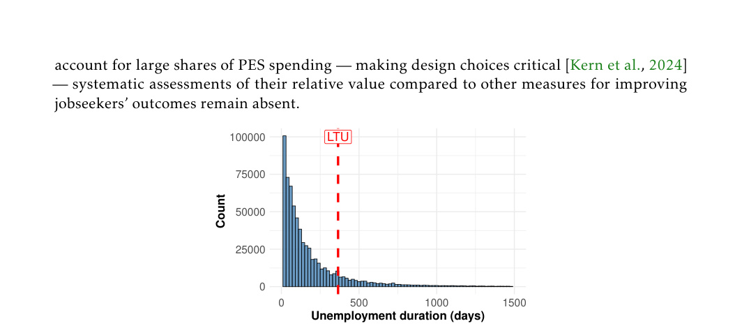
Figure 3: Unemployment duration The red line marks the 12 month threshold used to classify a jobseeking episode as long-term unemployment (LTU) in Germany.
图 3:失业时长。红线标出德国将求职期归类为长期失业(LTU)所用的 12 个月阈值。
We secured access to a dataset[^1] on German jobseekers derived from German administrative labor market records that cover a large portion of the German labor force. It covers a period from 1975 to 2017 and merges multiple administrative data sources, containing a wide spectrum of individual labor market information — including records on employment histories, received benefits, unemployment periods, participation in job training programs and demographic information. Such administrative records are the primary data source used by PES to build algorithmic profiling models [Bach et al., 2023].
我们获准使用来自德国行政劳动力市场记录、覆盖德国劳动力很大一部分的求职者数据集[^1]。覆盖 1975 至 2017 年,合并多源行政数据,含广泛个体劳动力市场信息——包括就业史、领取福利、失业期、参加就业培训与人口统计信息。此类行政记录是 PES 构建算法画像模型的主要数据源 [Bach et al., 2023]。
Experimental Setup.
We train a model to predict how long a newly registered jobseeker remains unemployed, defining the target as unemployment duration in days (capped at months)[^2]. Following Bach et al. [2023], we use a set of covariates capturing demographic information, labor market history, and most recent job details. We focus on unemployment spells beginning between 2010 and 2015, resulting in data on 274,515 different jobseekers and 553,980 unemployment spells (see Figure 4).
实验设置。
我们训练模型预测新登记求职者保持失业多久,将目标 定义为失业天数(封顶 个月)[^2]。遵循 Bach et al. [2023],使用捕获人口统计、劳动力市场史与最近工作细节的协变量集。聚焦 2010 至 2015 年开始的失业期,得到 274,515 名不同求职者与 553,980 段失业期(见图 4)。
To avoid the impact of significant labor market reforms in Germany and to ensure full observation of unemployment durations up to 24 months, we restrict our analysis to unemployment episodes that began between 2010 and 2015. We use records from 2010 and 2011 to build the training dataset, records from 2012 for validation, and evaluate test performance on data from 2015 (see Figure 4). We left a gap between the training and test data periods to allow enough time for the outcomes in the training data to have been fully observed at test time, in order to mimic a realistic deployment scenario starting at the beginning of 2015. We refer to Appendix B.1 for additional information on the experimental setup and data.
为避免德国重大劳动力市场改革影响,并确保可完整观察至 24 个月的失业时长,我们把分析限制在 2010 至 2015 年开始的失业事件。用 2010 与 2011 年记录建训练数据,2012 年做验证,在 2015 年数据上评估测试表现(见图 4)。训练与测试期之间留间隙,以便测试时训练数据中的结果已充分被观察,模拟 2015 年初开始的真实部署场景。实验设置与数据更多信息见附录 B.1。
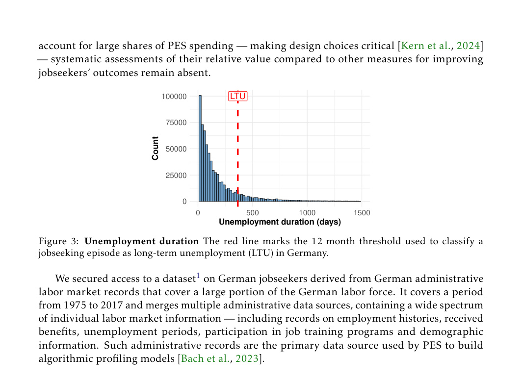
Figure 4: Stacked timeline diagram illustrating training (2010–2013), validation (2012–2014), and test (2015–2017) data periods. Red dashed boundaries within each colored box indicate the possible start dates of unemployment episodes, while the full colored boxes represent the entire observation phases for each dataset.
图 4:堆叠时间线图示,说明训练(2010–2013)、验证(2012–2014)与测试(2015–2017)数据时段。各色块内红色虚线边界表示失业事件可能开始日期,完整色块表示各数据集的整个观察期。
Guiding Questions
Our focus is the -fraction of jobseekers with the longest expected unemployment durations, representing those most at risk. In Germany, being unemployed for over one year (about of cases in our data; see Figure 3) meets the legal definition of long-term unemployment [Bach et al., 2023], but some countries adopt different cutoffs [Desiere et al., 2019]. Taking the perspective of a social planner designing a profiling system in a public employment office, our analysis aims to answer the following questions:
引导问题
我们聚焦预期失业时长最长的 比例求职者,代表风险最高者。在德国,失业超过一年(数据中约 的情形;见图 3)符合长期失业的法定定义 [Bach et al., 2023],但一些国家采用不同截止点 [Desiere et al., 2019]。站在公共就业办公室设计画像系统的社会规划者视角,我们的分析旨在回答以下问题:
- – How much does the screening capacity[^3] need to increase to ensure a significant portion of the high-risk jobseekers are screened, given the inaccuracies in the prediction system?
- – 在预测系统有误差的前提下,筛查能力[^3]需增大多少,才能确保相当比例的高风险求职者被筛查?
- – What is the real-world impact of improving screening capacity versus prediction errors?
- – 改进筛查能力相对预测误差的真实世界影响是什么?
- – When do small improvements in prediction error have the largest impact?
- – 预测误差的小改进何时影响最大?
- – What are the relative benefits and trade-offs of using a simpler vs more complex prediction model?
- – 使用更简单相对更复杂预测模型的相对收益与权衡是什么?
5.1 Results
5.1 结果
We train a CatBoost model (see Appendix B.2 for details), achieving an of on the test set. This level of predictive power aligns well with what is typically observed in social prediction tasks [Salganik et al., 2020] and similar applied settings [Desiere et al., 2019].
我们训练 CatBoost 模型(细节见附录 B.2),在测试集上达到 为 。该预测能力水平与社会预测任务中通常观察结果良好对齐 [Salganik et al., 2020],也与类似应用设定一致 [Desiere et al., 2019]。
How much does the screening capacity need to increase to target a significant fraction of high-risk jobseekers?
As expected, larger screening capacities increase both the policy value and the number of high-risk jobseekers screened (see Figure 5). Focusing on the (German) LTU cutoff (), our policy value aligns well with findings of previous studies[^4] [Bach et al., 2023].
筛查能力需增大多少才能瞄准显著比例的高风险求职者?
如预期,更大筛查能力同时提高策略价值与被筛查的高风险求职者人数(见图 5)。聚焦(德国)LTU 截止点(),我们的策略价值与既往研究发现良好对齐[^4] [Bach et al., 2023]。
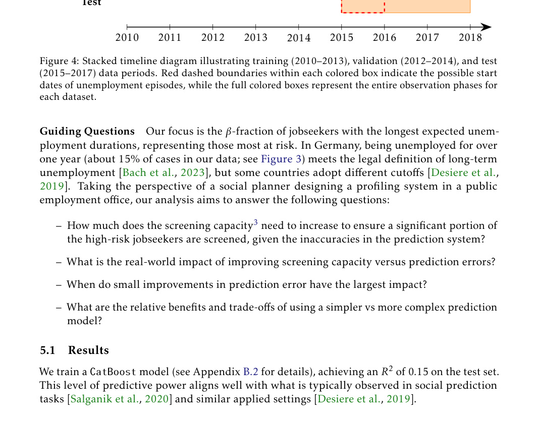
Figure 5: Policy value across different screening capacities () and worst-off fractions evaluated on the test set using the CatBoost regression model. A value of corresponds to the -month cutoff used to define long-term unemployment in Germany.
图 5:用 CatBoost 回归模型在测试集上评估的、跨不同筛查能力()与最弱势比例 的策略价值。 取值 对应德国定义长期失业的 个月截止点。
A planner might begin by setting , ensuring that, in theory, enough capacity is provided to screen and support every high-risk jobseeker. A natural question then arises: how much additional capacity would be required to screen at least a specified percentage of high-risk individuals? This additional capacity represents the overhead that must be invested to account for imperfect predictions. We observe that the required to ensure at least 75% of high-risk jobseekers are screened remains consistently around across different values. While the policy value increases as rises, the marginal improvements gained from increasing access decrease for higher , resulting in a somewhat stable across . In practice, this means we need to screen more of the population to ensure adequate coverage.
规划者可能先设 ,理论上确保有足够能力筛查并支持每位高风险求职者。自然问题随之而来:为至少筛查指定百分比的高风险个体,还需多少额外能力 ?该额外能力代表为计入不完美预测必须投入的开销。我们观察到:为确保至少 75% 高风险求职者被筛查所需的 跨不同 值大致稳定在 左右。虽策略价值随 上升而增大,但更高 下增大接入的边际改进下降,使跨 的 相对稳定。实践中这意味着需多筛查人口的 才能确保充分覆盖。
(a) Constant Prediction ()
(a) 常数预测()
What is the impact of improving screening capacity versus prediction errors?
We simulate small improvements in the value by uniformly scaling the residuals by a multiplicative factor.
改进筛查能力相对预测误差的影响是什么?
我们通过用乘性因子均匀缩放残差来模拟 值的小改进。
To ensure that this approach approximates a realistic pathway of (marginally) improving the model, we train various models at different sample sizes. We then verify that as increases with the amount of training data, the variance of the residuals decreases, while the distribution remains largely unchanged in shape (see Figure 13). We then evaluate the prediction-access ratio for in three scenarios : (1) the trained CatBoost model with , (2) near-perfect predictions with and (3) constant predictions (), effectively randomizing screening decisions.
为确保该方法近似(边际)改进模型的现实路径,我们在不同样本量上训练多种模型。随后验证:随着训练数据量增加, 上升时残差方差下降,而分布形状大体不变(见图 13)。接着在三种情形下评估 的预测–接入比:(1) 训练得到的 CatBoost 模型,;(2) 近乎完美预测,;(3) 常数预测(),实质上随机化筛查决策。
We observe a rise in the PAR for small screening capacities (see Figure 6), consistent with Theorem 3.1. Under random allocation (), the PAR stays below one for . This result aligns somewhat with Theorem 3.2, where we found that the (local) PAR approaches zero as . Because we consider (rather than an infinitesimal improvement, see Figure 14 for ), the PAR remains large at small . For the CatBoost model (), capacity improvements stay relatively more effective (i.e., PAR ) for larger , matching Proposition 3, where we found that for moderate and , the local PAR remains above one. Meanwhile, near-perfect predictions () make capacity investments highly efficient, causing the PAR to diverge for , then drop sharply near because the allocation becomes nearly optimal. When , the PAR stabilizes at one as numerator and denominator both approach zero.
我们观察到小筛查能力 下 PAR 上升(见图 6),与定理 3.1 一致。在随机分配()下,对 ,PAR 保持低于一。这与定理 3.2 部分对齐——我们曾发现当 时(局部)PAR 趋于零。因我们取 (而非无穷小改进,见图 14 中 ),小 处 PAR 仍较大。对 CatBoost 模型(),在更大 下能力改进仍相对更有效(即 PAR ),与命题 3 吻合——对中等 且 ,局部 PAR 保持高于一。同时,近乎完美预测()使能力投资高度高效,导致 时 PAR 发散,随后在 附近急剧下降,因为分配已近乎最优。当 时,分子分母都趋于零,PAR 稳定在一。
These observations broadly match our theoretical findings, despite the non-local improvements and more complex residual structure. Notably, the theory’s focus on local improvements offers a conservative perspective on capacity investments: even under random allocation (), securing a modest screening capacity () is often the first priority, while at very high , gains in policy value diminish so rapidly once that the relative advantage of further prediction investments becomes negligible.
这些观察与理论发现大体吻合,尽管改进非局部、残差结构更复杂。值得注意的是,理论聚焦局部改进,对能力投资给出偏保守视角:即便在随机分配()下,先确保适度筛查能力()往往是第一优先;而在很高 下,一旦 ,策略价值增益迅速衰减,进一步预测投资的相对优势变得可忽略。
When do small improvements in prediction error have the largest impact?
From theory (Theorem 3.2), we expect local policy value improvements from better predictions to diverge as and when . This aligns with our results in Figure 7: for small , the rate of local improvements in with respect to diverges. The location of the maximum in also follows from the theory: as , the rate only diverges for , while for small the maximum is at .
预测误差的小改进何时影响最大?
由理论(定理 3.2),我们期望更好预测带来的局部策略价值改进在 以及当 时 处发散。这与图 7 结果一致:对小 , 对 的局部改进率发散。 上最大值的位置也遵循理论:当 时,该率仅在 发散;而对小 ,最大值约在 。
(a)
What are the relative benefits and trade-offs of using a simpler vs more complex prediction model?
We compare a shallow 4-depth decision tree with the CatBoost model. As expected, the simpler tree shows a small drop in predictive power ( decrease in ) which translates into a – reduction in policy value (see Figure 8(a)). Compared to a uniform increase in achieved by scaling the residuals (see Figure 15), the differences in policy value are only partially similar across . The CatBoost model does not provide a uniform improvement over the decision tree; for instance, it performs better at distinguishing longer unemployment spells.
使用更简单相对更复杂预测模型的相对收益与权衡是什么?
我们比较深度为 4 的浅决策树与 CatBoost 模型。如预期,更简单的树预测能力略降( 下降 ),转化为策略价值减少 –(见图 8(a))。与通过缩放残差实现的均匀 提升相比(见图 15),跨 的策略价值差异仅部分相似。CatBoost 相对决策树并非提供均匀改进;例如,它在区分更长失业期上表现更好。
Despite this performance gap, the simpler model offers potential advantages: it fits on a single sheet of paper, demands minimal computational infrastructure, can be easily explained to frontline case workers and resembles the categorical prioritization rules common in public institutions. [Johnson and Zhang, 2022]. Because more complex models incur higher costs, a planner might instead increase screening capacity. Formally, we define
尽管存在该表现差距,更简单模型仍有潜在优势:可写在一张纸上,几乎不需计算基础设施,易于向一线个案工作者解释,并类似公共机构常见的类别优先规则 [Johnson and Zhang, 2022]。因更复杂模型成本更高,规划者或可改为增大筛查能力。形式上,我们定义
the smallest that matches the policy-value gains of the CatBoost model. Empirically, mostly rises with (see Figure 8(b)), consistent with our finding that the PAR decreases with . By framing the difference between models in terms of additional screenings, planners can directly compare the cost of increased capacity to that of deploying a more complex model.
能匹配 CatBoost 模型策略价值增益的最小 。经验上, 大体随 上升(见图 8(b)),与我们关于 PAR 随 下降的发现一致。把模型差异表述为额外筛查次数,规划者可直接比较增大能力的成本与部署更复杂模型的成本。
(a) Difference in Policy Value
(a) 策略价值差异
6 Conclusion
6 结论
This paper develops a framework for quantifying the relative value of prediction in identifying the worst-off. We formalize tradeoffs between expanding screening capacity and improving predictive models, and show through both mathematical analysis and a real-world case study that prediction is not always the most important piece of the puzzle in social allocation systems. Future work could examine more specific application settings and cost structures, including distinctions between fixed and recurring costs, and explore policy levers that improve prediction unevenly, for example, by reducing errors in high-risk subgroups or by increasing robustness to distributional shifts. More broadly, we see a need for clearer theoretical foundations to understand the role of prediction in public-sector allocation, particularly in relation to the institutional and administrative systems in which it is embedded.
本文建立量化预测在识别最弱势群体中相对价值的框架。我们形式化扩展筛查能力与改进预测模型之间的权衡,并通过数学分析与真实案例研究表明:在社会分配系统中,预测并不总是拼图中最重要的一块。未来工作可考察更具体的应用设定与成本结构——包括固定与经常性成本的区分——并探索对预测改进不均的政策杠杆,例如降低高风险子群误差,或增强对分布漂移的稳健性。更广地看,我们需要更清晰的理论基础,以理解预测在公共部门分配中的角色,特别是相对其所嵌入的制度与行政系统。
Acknowledgements
This work is supported by the DAAD programme Konrad Zuse Schools of Excellence in Artificial Intelligence, sponsored by the Federal Ministry of Education and Research and by the Volkswagen Foundation, grant “Consequences of Artificial Intelligence for Urban Societies (CAIUS)”. Juan Carlos Perdomo is supported by the Center for Research on Computation and Society (CRCS) at Harvard University and by the Alfred P. Sloan Foundation grant G-2020-13941. We would like to thank the anonymous reviewers for their insightful comments, as well as Frauke Kreuter, Patrick Schenk and Moritz Hardt for their valuable feedback.
References
Aiken et al. [2023] E. Aiken, T. Ohlenburg, and J. Blumenstock. Moving targets: When does a poverty prediction model need to be updated? In Proceedings of the 6th ACM SIGCAS/SIGCHI Conference on Computing and Sustainable Societies , COMPASS ’23, page 117, New York, NY, USA, 2023. Association for Computing Machinery. ISBN 9798400701498. doi: 10.1145/3588001.3609369 . URL https://doi.org/10.1145/3588001.3609369 .
Antoni et al. [2019a] M. Antoni, A. Ganzer, and P. vom Berge. Factually anonymous version of the Sample of Integrated Labour Market Biographies (SIAB-Regionalfile) – Version 7517 v1. Research Data Centre of the Federal Employment Agency (BA) at the Institute for Employment Research (IAB), 2019a. 10.5164/IAB.SIAB-R7517.de.en.v1.
Antoni et al. [2019b] M. Antoni, A. Ganzer, and P. vom Berge. Sample of Integrated Labour Market Biographies Regional File (SIAB-R) 1975 - 2027. FDZ-Datenreport 04/2019 (en), Research Data Centre of the Federal Employment Agency (BA) at the Institute for Employment Research (IAB), Nürnberg, 2019b. 10.5164/IAB.FDZD.1904.en.v1.
Athey and Wager [2021] S. Athey and S. Wager. Policy Learning with Observational Data. Econometrica , 89(1):133–161, 2021.
Bach et al. [2023] R. L. Bach, C. Kern, H. Mautner, and F. Kreuter. The impact of modeling decisions in statistical profiling. Data & Policy , 5:e32, 2023. doi: 10.1017/dap.2023.29 .
Barocas et al. [2023] S. Barocas, M. Hardt, and A. Narayanan. Fairness and Machine Learning: Limitations and Opportunities . MIT Press, 2023.
Blumenstock [2016] J. E. Blumenstock. Fighting Poverty with Data. Science , 2016.
Boehmer et al. [2024] N. Boehmer, Y. Nair, S. Shah, L. Janson, A. Taneja, and M. Tambe. Evaluating the Effectiveness of Index-Based Treatment Allocation. arXiv preprint arXiv:2402.11771 , 2024.
Chan et al. [2012] C. W. Chan, V. F. Farias, N. Bambos, and G. J. Escobar. Optimizing Intensive Care Unit Discharge Decisions with Patient Readmissions. Operations Research , 60(6):1323–1341, 2012. doi: 10.1287/opre.1120.1105 . URL https://doi.org/10.1287/opre.1120.1105 .
Chouldechova et al. [2018] A. Chouldechova, D. Benavides-Prado, O. Fialko, and R. Vaithianathan. A case study of algorithm-assisted decision making in child maltreatment hotline screening decisions. In Conference on Fairness, Accountability and Transparency , pages 134–148. PMLR, 2018.
Clementi and Gallegati [2005] F. Clementi and M. Gallegati. Pareto’s law of income distribution: Evidence for Germany, the United Kingdom, and the United States. Econophysics of wealth distributions: Econophys-Kolkata I , pages 3–14, 2005.
Coston et al. [2023] A. Coston, A. Kawakami, H. Zhu, K. Holstein, and H. Heidari. A Validity Perspective on Evaluating the Justified Use of Data-driven Decision-making Algorithms. In 2023 IEEE Conference on Secure and Trustworthy Machine Learning (SaTML) , pages 690–704, 2023. doi: 10.1109/SaTML54575.2023.00050 .
Desiere and Struyven [2021] S. Desiere and L. Struyven. Using Artificial Intelligence to classify Jobseekers: The Accuracy-Equity Trade-off. Journal of Social Policy , 50(2):367–385, Apr. 2021. ISSN 0047-2794, 1469-7823. doi: 10.1017/S0047279420000203 .
Desiere et al. [2019] S. Desiere, K. Langenbucher, and L. Struyven. Statistical Profiling in Public Employment Services: An International Comparison. Technical Report 224, OECD Publishing, 2019. URL https://doi.org/10.1787/b5e5f16e-en .
Drezner and Wesolowsky [1990] Z. Drezner and G. O. Wesolowsky. On the Computation of the Bivariate Normal Integral. Journal of Statistical Computation and Simulation , 1990.
Elmachtoub and Grigas [2022] A. N. Elmachtoub and P. Grigas. Smart “predict, then optimize”. Management Science , 68(1):9–26, 2022.
Fernández-Loría and Provost [2022] C. Fernández-Loría and F. Provost. Causal Decision Making and Causal Effect Estimation Are Not the Same…and Why It Matters. INFORMS Journal on Data Science , 1(1):4–16, 2022. doi: 10.1287/ijds.2021.0006 . URL https://doi.org/10.1287/ijds.2021.0006 .
Fischer-Abaigar et al. [2024] U. Fischer-Abaigar, C. Kern, N. Barda, and F. Kreuter. Bridging the Gap: Towards an Expanded Toolkit for Ai-driven Decision-making in the Public Sector. Government Information Quarterly , 41(4):101976, 2024. ISSN 0740-624X. doi: https://doi.org/10.1016/j.giq.2024.101976 . URL https://www.sciencedirect.com/science/article/pii/S0740624X24000686 .
Guerdan et al. [2023] L. Guerdan, A. Coston, K. Holstein, and Z. S. Wu. Counterfactual Prediction Under Outcome Measurement Error. In Proceedings of the 2023 ACM Conference on Fairness, Accountability, and Transparency , FAccT ’23, page 1584–1598, New York, NY, USA, 2023. Association for Computing Machinery. ISBN 9798400701924. doi: 10.1145/3593013.3594101 . URL https://doi.org/10.1145/3593013.3594101 .
Jain et al. [2024] S. Jain, K. Creel, and A. C. Wilson. Position: Scarce Resource Allocations That Rely On Machine Learning Should Be Randomized. In Forty-first International Conference on Machine Learning , 2024. URL https://openreview.net/forum?id=44qxX6Ty6F .
Johnson and Zhang [2022] R. A. Johnson and S. Zhang. What is the Bureaucratic Counterfactual? Categorical versus Algorithmic Prioritization in U.S. Social Policy. In Proceedings of the 2022 ACM Conference on Fairness, Accountability, and Transparency , FAccT ’22, page 1671–1682, New York, NY, USA, 2022. Association for Computing Machinery. ISBN 9781450393522. doi: 10.1145/3531146.3533223 . URL https://doi.org/10.1145/3531146.3533223 .
Kallus [2021] N. Kallus. More Efficient Policy Learning via Optimal Retargeting. Journal of the American Statistical Association , 116(534):646–658, 2021. doi: 10.1080/01621459.2020.1788948 . URL https://doi.org/10.1080/01621459.2020.1788948 .
Kern et al. [2024] C. Kern, R. Bach, H. Mautner, and F. Kreuter. When Small Decisions Have Big Impact: Fairness Implications of Algorithmic Profiling Schemes. ACM Journal on Responsible Computing , 1(4), Nov. 2024. doi: 10.1145/3689485 . URL https://doi.org/10.1145/3689485 .
Kitagawa and Tetenov [2018] T. Kitagawa and A. Tetenov. Who Should Be Treated? Empirical Welfare Maximization Methods for Treatment Choice. Econometrica , 86(2):591–616, 2018. doi: https://doi.org/10.3982/ECTA13288 . URL https://onlinelibrary.wiley.com/doi/abs/10.3982/ECTA13288 .
Kleinberg et al. [2015] J. Kleinberg, J. Ludwig, S. Mullainathan, and Z. Obermeyer. Prediction Policy Problems. American Economic Review , 105(5):491–495, 2015.
Körtner and Bonoli [2023] J. Körtner and G. Bonoli. Predictive Algorithms in the Delivery of Public Employment Services. In Handbook of Labour Market Policy in Advanced Democracies , pages 387–398. Edward Elgar Publishing, 2023.
Loxha and Morgandi [2014] A. Loxha and M. Morgandi. Profiling the unemployed: a review of OECD experiences and implications for emerging economics. Social protection discussion papers and notes , (91051), 2014.
Manski [2004] C. F. Manski. Statistical Treatment Rules for Heterogeneous Populations. Econometrica , 72(4):1221–1246, 2004. doi: https://doi.org/10.1111/j.1468-0262.2004.00530.x . URL https://onlinelibrary.wiley.com/doi/abs/10.1111/j.1468-0262.2004.00530.x .
Perdomo [2024] J. C. Perdomo. The Relative Value of Prediction in Algorithmic Decision Making. In Proceedings of the 41st International Conference on Machine Learning , ICML’24. JMLR.org, 2024.
Perdomo et al. [2023] J. C. Perdomo, T. Britton, M. Hardt, and R. Abebe. Difficult Lessons on Social Prediction from Wisconsin Public Schools. arXiv preprint arXiv:2304.06205 , 2023.
Potash et al. [2015] E. Potash, J. Brew, A. Loewi, S. Majumdar, A. Reece, J. Walsh, E. Rozier, E. Jorgenson, R. Mansour, and R. Ghani. Predictive Modeling for Public Health: Preventing Childhood Lead Poisoning. In Proceedings of the 21th ACM SIGKDD International Conference on Knowledge Discovery and Data Mining , KDD ’15, page 2039–2047, New York, NY, USA, 2015. Association for Computing Machinery. ISBN 9781450336642. doi: 10.1145/2783258.2788629 . URL https://doi.org/10.1145/2783258.2788629 .
Salganik et al. [2020] M. J. Salganik, I. Lundberg, A. T. Kindel, C. E. Ahearn, K. Al-Ghoneim, A. Almaatouq, D. M. Altschul, J. E. Brand, N. B. Carnegie, R. J. Compton, D. Datta, T. Davidson, A. Filippova, C. Gilroy, B. J. Goode, E. Jahani, R. Kashyap, A. Kirchner, S. McKay, A. C. Morgan, A. Pentland, K. Polimis, L. Raes, D. E. Rigobon, C. V. Roberts, D. M. Stanescu, Y. Suhara, A. Usmani, E. H. Wang, M. Adem, A. Alhajri, B. AlShebli, R. Amin, R. B. Amos, L. P. Argyle, L. Baer-Bositis, M. Büchi, B.-R. Chung, W. Eggert, G. Faletto, Z. Fan, J. Freese, T. Gadgil, J. Gagné, Y. Gao, A. Halpern-Manners, S. P. Hashim, S. Hausen, G. He, K. Higuera, B. Hogan, I. M. Horwitz, L. M. Hummel, N. Jain, K. Jin, D. Jurgens, P. Kaminski, A. Karapetyan, E. H. Kim, B. Leizman, N. Liu, M. Möser, A. E. Mack, M. Mahajan, N. Mandell, H. Marahrens, D. Mercado-Garcia, V. Mocz, K. Mueller-Gastell, A. Musse, Q. Niu, W. Nowak, H. Omidvar, A. Or, K. Ouyang, K. M. Pinto, E. Porter, K. E. Porter, C. Qian, T. Rauf, A. Sargsyan, T. Schaffner, L. Schnabel, B. Schonfeld, B. Sender, J. D. Tang, E. Tsurkov, A. van Loon, O. Varol, X. Wang, Z. Wang, J. Wang, F. Wang, S. Weissman, K. Whitaker, M. K. Wolters, W. L. Woon, J. Wu, C. Wu, K. Yang, J. Yin, B. Zhao, C. Zhu, J. Brooks-Gunn, B. E. Engelhardt, M. Hardt, D. Knox, K. Levy, A. Narayanan, B. M. Stewart, D. J. Watts, and S. McLanahan. Measuring the Predictability of Life Outcomes with a Scientific Mass Collaboration. Proceedings of the National Academy of Sciences , 117(15):8398–8403, 2020. doi: 10.1073/pnas.1915006117 . URL https://www.pnas.org/doi/abs/10.1073/pnas.1915006117 .
Shirali et al. [2024] A. Shirali, R. Abebe, and M. Hardt. Allocation Requires Prediction Only if Inequality Is Low. In Forty-first International Conference on Machine Learning, ICML 2024, Vienna, Austria, July 21-27, 2024 . OpenReview.net, 2024. URL https://openreview.net/forum?id=WUicA0hOF9 .
Sun and Medaglia [2019] T. Q. Sun and R. Medaglia. Mapping the challenges of Artificial Intelligence in the public sector: Evidence from public healthcare. Government Information Quarterly , 36(2):368–383, 2019.
Wang et al. [2024] A. Wang, S. Kapoor, S. Barocas, and A. Narayanan. Against Predictive Optimization: On the Legitimacy of Decision-making Algorithms That Optimize Predictive Accuracy. ACM J. Responsib. Comput. , 1(1), Mar. 2024. doi: 10.1145/3636509 . URL https://doi.org/10.1145/3636509 .
Wilder and Welle [2024] B. Wilder and P. Welle. Learning treatment effects while treating those in need. arXiv preprint arXiv:2407.07596 , 2024.
Wirtz et al. [2019] B. W. Wirtz, J. C. Weyerer, and C. Geyer. Artificial Intelligence and the Public Sector—Applications and Challenges. International Journal of Public Administration , 42(7):596–615, 2019.
Appendix A Theoretical Investigation
附录 A 理论考察
(a) Normal Welfare Distribution
(a) 正态福利分布
(a) PAR
Appendix B Experiments
附录 B 实验
B.1 Experimental Setup and Labor Market Data
B.1 实验设置与劳动力市场数据
The dataset is provided via a Scientific Use File by the Research Data Centre (FDZ) of the German Federal Employment Agency (BA) at the Institute for Employment Research (IAB) [Antoni et al., 2019a, Antoni et al., 2019b]. It is a weakly anonymized random sample of the complete German labor market records from 1975 to 2017 and contains information on 1,827,903 individuals across 62,340,521 observations [Antoni et al., 2019b].
数据集由德国联邦就业局(BA)就业研究所(IAB)研究数据中心(FDZ)以科学使用文件形式提供 [Antoni et al., 2019a, Antoni et al., 2019b]。它是 1975 至 2017 年完整德国劳动力市场记录的 弱匿名随机样本,覆盖 1,827,903 人、共 62,340,521 条观测 [Antoni et al., 2019b]。
We follow the same set of covariates and aggregation procedure for individual unemployment spells as described in Bach et al. [2023], incorporating demographic characteristics, labor market histories, and information about the most recent job. This results in 56 numerical variables and 24 categorical variables, which are one-hot encoded for model training. Figure 3 shows a histogram of individual unemployment durations, which we use as the basis for constructing the outcome variables. The distribution is right-skewed, with a concentration on short durations near zero and a long tail. Such a pattern is commonly observed in other welfare-related outcomes, such as health or income metrics. We define as prediction target the duration of the unemployment period in days , capped at months[^5]. Differentiating tail values is less important for decision-making, and capping also allows training across years with varying observation windows.
我们遵循 Bach et al. [2023] 所述协变量集与个体失业期聚合流程,纳入人口统计特征、劳动力市场史与最近工作信息。得到 56 个数值变量与 24 个类别变量,训练时做独热编码。图 3 给出个体失业时长直方图,作为构建结果变量的基础。分布右偏,短时长集中在零附近并有长尾。该模式在健康或收入等其他福利相关结果中也常见。我们将预测目标定义为失业天数 ,封顶 个月[^5]。区分尾部值对决策较不重要,封顶也便于在观察窗口不同的年份间训练。
B.2 Training Details
B.2 训练细节
We use CatBoost (https://catboost.ai) for model training. The model was trained for a maximum 5,000 iterations with an early stopping criterion (early_stopping_rounds = 20) based on validation performance. Additionally, we train a shallow Decision Tree (max_depth = 4) using the scikit-learn package. All hyperparameters are kept at their default settings unless otherwise specified.
我们用 CatBoost(https://catboost.ai)训练模型。最大迭代 5,000 次,并按验证表现设置早停(early_stopping_rounds = 20)。另外用 scikit-learn 训练浅决策树(max_depth = 4)。除非另说明,所有超参数保持默认。
B.3 Prediction Improvements
B.3 预测改进
To simulate an increase in predictive power by a specified amount , we adjust the model’s predictions using the residuals . Starting with the original predictions and true outcomes , we define the adjusted predictions as
为模拟预测能力增加指定量 ,我们用残差 调整模型预测 。从原始预测 与真实结果 出发,定义调整后的预测为
We can then determine the corresponding to an increase of in the model’s :
随后可确定使模型 增加 所对应的 :
For a specified , the new residuals are
对给定 ,新残差为
Consequently, the variance decreases by a multiplicative factor: .
因而方差按乘性因子下降:。
(a)
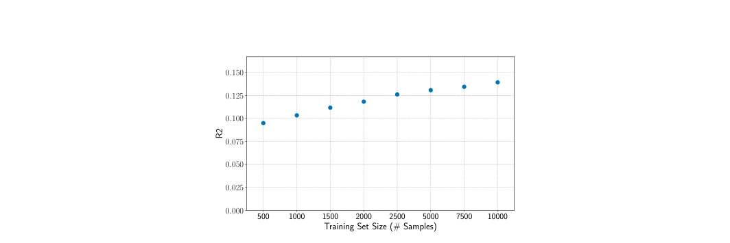
Figure 12: The value on the test set for varying training set size (CatBoost Regression).
图 12:不同训练集规模下测试集 值(CatBoost 回归)。
(a) Training Samples
(a) 个训练样本
B.4 Additional Figures
B.4 补充图
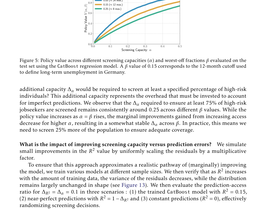
Figure 14: Prediction-Access Ratio for and .
图 14: 且 时的预测–接入比。
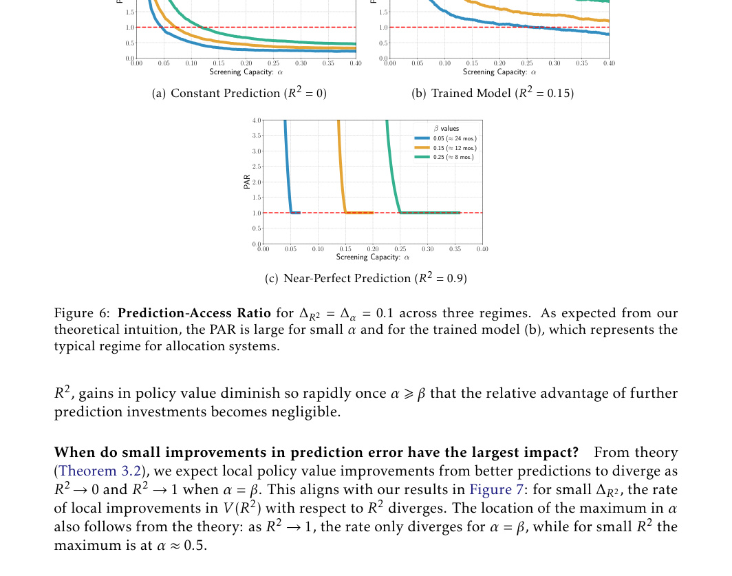
Figure 15: for CatBoost model and .
图 15:CatBoost 模型上 ,。
B.5 Binary Classification
B.5 二分类
Instead of predicting the exact duration of unemployment, the problem can be reframed as a binary classification task. For a fixed , we can define a binary outcome: . This approach more directly encodes the target of interest: identifying individuals who may require further screening or assistance. If the chosen classifier provides estimates of class probabilities , it can be used to formulate a decision policy . However, this forces us to specify and the resulting decision threshold prior to model training. This requirement reduces flexibility compared to a continuous prediction setup, making classification more appropriate when the model is not intended for use in other tasks and when remains constant across the deployment context. Additionally, directly converting durations to labels discards information on the precise unemployment durations that could be valuable for the modeling process.
除预测确切失业时长外,也可把问题重述为二分类。对固定 ,可定义二元结果:。该做法更直接编码关注目标:识别可能需进一步筛查或援助的个体。若所选分类器给出类概率估计 ,可用于形成决策策略 。但这迫使我们在模型训练前指定 与所得决策阈值。相对连续预测设定,该要求降低灵活性,使分类更适合模型不拟用于其他任务、且部署语境中 保持不变的情形。此外,直接把时长转为标签会丢弃对建模可能有价值的精确失业时长信息。
As can be seen in Figure 16, the resulting policy values and true positive counts remain very similar compared to the regression case.
如图 16 所示,所得策略价值与真正例计数相对回归情形仍非常相似。
(a) Policy Value
(a) 策略价值
Appendix C Additional Propositions
附录 C 补充命题
Proposition 4.
(Optimal Policy with Gaussian Errors) If and , then the optimal policy $\pi^{}\colon\mathbb{R}\to{0,1}$ to solve the screening problem (Definition 2.1) is equal to:*
命题 4。
(高斯误差下的最优策略)若 且 ,则解决筛查问题(定义 2.1)的最优策略 $\pi^{}\colon\mathbb{R}\to{0,1}$ 等于:*
where is the -quantile of . The value of the policy is $V(\pi^{})=\mathrm{Pr}[\hat{Y}\leqslant F^{-1}{\hat{Y}}(\alpha)\mid Y\leqslant F^{-1}{Y}(\beta)]$.*
其中 是 的 -分位数。策略价值为 $V(\pi^{})=\mathrm{Pr}[\hat{Y}\leqslant F^{-1}{\hat{Y}}(\alpha)\mid Y\leqslant F^{-1}{Y}(\beta)]$。*
Proof.
Since where and , it follows for the conditional distribution . Since is Gaussian, we can express the conditional probability from Proposition 1 in terms of the CDF of the standard normal distribution,
证明。
由于 ,其中 且 ,条件分布 。因 为高斯,可用标准正态 CDF 表达命题 1 中的条件概率,
To reproduce the ranking induced by , individuals can be ranked in ascending order of . Thus, we can express the optimal policy (Proposition 1) in terms of a ranking of ,
为再现 诱导的排序,可按 升序排列个体。因而可用 的排序表达最优策略(命题 1),
where is the -quantile of . The value that can by achieved by the optimal screening policy can then be expressed as:
其中 是 的 -分位数。最优筛查策略 可达成的价值 可表为:
∎
Appendix D Proofs
附录 D 证明
D.1 Optimal Policy for Screening Problem: Proof of Proposition 1
D.1 筛查问题最优策略:命题 1 的证明
Proof.
We rewrite the policy value,
证明。
我们改写策略价值,
To maximize the objective, individuals with the largest scores should be prioritized. Thus, the optimal policy is to intervene () for the top -fraction of the population ranked by . ∎
为最大化目标,应按分数 最大者优先考虑个体 。因而最优策略是对按 排序后人口顶部 比例实施干预()。∎
D.2 Optimal Policy Value in Gaussian Setting: Proof of Proposition 2
D.2 高斯设定下的最优策略价值:命题 2 的证明
Following Proposition 4, the value of the optimal screening policy can then be expressed as:
遵循命题 4,最优筛查策略 的价值可表为:
We can rewrite the conditional probability in terms of the joint distribution of and , and note that ,
可将条件概率改写为 与 的联合分布,并注意 ,
We then standardize and and make use that for a normal random variable with mean and variance the quantile function is .
随后标准化 与 ,并利用均值 、方差 的正态随机变量分位函数为 。
and are standard Gaussian with . Thus, they are distributed according to a standard bivariate normal distribution with correlation . Thus,
与 为标准高斯,且 。因而它们服从相关为 的标准二元正态分布。于是,
where
其中
and
以及
D.3 Prediction-Access Ratio for Small Screening Capacities: Proof of Theorem 3.1
D.3 小筛查能力下的预测–接入比:定理 3.1 的证明
Using Taylor’s theorem,
利用泰勒定理,
where . We know from Lemma D.3,
其中 。由引理 D.3 可知,
where . For and , we know and . It follows, that for any , and , there exists a threshold value , such that for all , we have
其中 。对 且 ,有 且 。由此,对任意 、 与 ,存在阈值 ,使得对所有 ,有
If we find . Since for ,
若 ,则 。由于对 有 ,
where . For any , there exists a threshold , such that for all , we can apply Lemma B.5. from Perdomo [2024] to arrive at the following inequality:
其中 。对任意 ,存在阈值 ,使得对所有 ,可应用 Perdomo [2024] 的 Lemma B.5.,得到不等式:
Thus,
因此,
We can use Taylor’s theorem again and from Lemma D.1 we know that
可再次使用泰勒定理,并由引理 D.1 可知
where . Since and there will always be a small enough such that
其中 。由于 且 ,总能取足够小的 使得
Since for , it follows
由于对 有 ,因而
It follows for the prediction-access ratio,
于是对预测–接入比有,
For small , grows asymptotically like . Consequently, the polynomial growth of drives the PAR to increase rapidly as decreases. Since increases with and , we can lower bound the PAR by inserting instead of :
对小 , 渐近像 增长。因而 的多项式增长驱动 PAR 随 减小而快速增大。由于 随 增大,且 ,可用 代替 给出 PAR 下界:
We can simplify the lower-bound by noting that and can be made arbitrarily small by selecting a sufficiently small threshold for . Specifically, holds for (see Lemma A.6 in Perdomo [2024]).
可通过选取足够小的 阈值 ,使 、 任意小,从而简化下界。具体地,对 有 (见 Perdomo [2024] 的 Lemma A.6)。
D.4 Maximally Effective (Local) Prediction Improvements: Proof of Theorem 3.2
D.4 最有效的(局部)预测改进:定理 3.2 的证明
We know from Lemma D.2,
由引理 D.2 可知,
We insert and arrive at
代入 得到
The prefactor diverges as or .
前因子 在 或 时发散。
If , the exponential term will generally suppress the polynomial growth of the prefactor. However for , we find for the exponent
若 ,指数项通常会压制前因子的多项式增长。但对 ,指数满足
which is finite. Therefore, becomes unboundedly large if and .
其为有限。因此,当 且 时, 变得无界大。
If , the prefector diverges again to . The exponent then simplifies to
若 ,前因子 再次发散至 。指数则简化为
If and are not set arbitrarily small or large will diverge. The local PAR (Lemma D.1)
若 与 未设得任意小或任意大,则 会发散。局部 PAR(引理 D.1)
approaches zero in both regimes.
在两体制下都趋于零。
D.5 Prediction-Access Ratio for Local Improvements: Proof of Proposition 3
D.5 局部改进的预测–接入比:命题 3 的证明
We know
我们有
Using Lemma D.1 and Lemma D.3 we find a lower bound for the PAR:
利用引理 D.1 与引理 D.3,得到 PAR 的下界:
We then denote and . We know from Lemma D.4 that increases with . It follows that we need to find the smallest possible to find a lower bound for . Generally, decreases with and increases with . We treat both cases separately:
记 ,。由引理 D.4, 随 增大。因而需找尽可能小的 以得到 下界。一般地, 随 减小、随 增大。我们分开处理两种情形:
- For we find . Since decreases with and we can lower bound the expression by setting and . Thus, and . Since we can lower bound the prefactor .
- 对 ,有 。由于 随 减小且 ,可取 、 得到下界。因而 且 。又因 ,前因子满足 。
- For , it follows by setting . Since and , it follows and
- 对 ,取 ,有 。由于 且 ,因而 且 。
In both cases, we can combine the lower bounds of and to find
两种情形下,均可合并 与 的下界得到
D.6 Technical Lemmas
D.6 技术引理
Lemma D.1(Derivative w.r.t. ).
Lemma D.1(Derivative w.r.t. ).
Proof.
In the Gaussian setting we find for the policy value (Proposition 2),
证明。
在高斯设定下,策略价值(命题 2)为
We first apply Leibniz integral rule,
先应用莱布尼茨积分法则,
We insert the bivariate density and substitute
代入二元密度 ,并做替换
∎
Lemma D.2(Derivative w.r.t. ).
Lemma D.2(Derivative w.r.t. ).
where is the standard bivariate density.
其中 是标准二元密度。
Proof.
where is the standard bivariate density. We utilized , and in the final step applied the partial derivative of the standard bivariate cumulative distribution with respect to its correlation [Drezner and Wesolowsky, 1990]. ∎
其中 是标准二元密度。我们利用了 ,并在最后一步应用了标准二元累积分布对其相关 的偏导数 [Drezner and Wesolowsky, 1990]。∎
Lemma D.3(Upper bound of derivative).
Let . Then,
引理 D.3( 导数的上界)。
令 。则
Proof.
We know from Lemma D.2,
证明。
由引理 D.2 可知,
Since ,
由于 ,
Similarly,
类似地,
Thus,
因此,
and
以及
∎
Lemma D.4.
The ratio
引理 D.4。
比值
is increasing in .
关于 递增。
Proof.
We compute the derivative of the ratio ,
证明。
计算比值 的导数,
For the derivative is clearly positive. For we start by rewriting,
对 ,导数显然为正。对 ,先改写为
Since and , it follows for that . Thus for any ,
由于 ,且 ,因而对 有 。于是对任意 ,
∎