UNITER: UNiversal Image-TExt Representation Learning
UNITER: UNiversal Image-TExt Representation Learning
UNITER:通用图像-文本表征学习
Yen-Chun Chen † † thanks: Equal contribution. Linjie Li ⋆ Licheng Yu ⋆ Ahmed El Kholy Faisal Ahmed Zhe Gan Yu Cheng Jingjing Liu Affiliation: Microsoft Dynamics 365 AI Research E-mail {yen-chun.chen,lindsey.li,licheng.yu,ahmed.elkholy,fiahmed, zhe.gan,yu.cheng,jingjl}@microsoft.com
Abstract
摘要
Joint image-text embedding is the bedrock for most Vision-and-Language (V+L) tasks, where multimodality inputs are simultaneously processed for joint visual and textual understanding. In this paper, we introduce UNITER, a UNiversal Image-TExt Representation, learned through large-scale pre-training over four image-text datasets (COCO, Visual Genome, Conceptual Captions, and SBU Captions), which can power heterogeneous downstream V+L tasks with joint multimodal embeddings. We design four pre-training tasks: Masked Language Modeling (MLM), Masked Region Modeling (MRM, with three variants), Image-Text Matching (ITM), and Word-Region Alignment (WRA). Different from previous work that applies joint random masking to both modalities, we use conditional masking on pre-training tasks (i.e., masked language/region modeling is conditioned on full observation of image/text). In addition to ITM for global image-text alignment, we also propose WRA via the use of Optimal Transport (OT) to explicitly encourage fine-grained alignment between words and image regions during pre-training. Comprehensive analysis shows that both conditional masking and OT-based WRA contribute to better pre-training. We also conduct a thorough ablation study to find an optimal combination of pre-training tasks. Extensive experiments show that UNITER achieves new state of the art across six V+L tasks (over nine datasets), including Visual Question Answering, Image-Text Retrieval, Referring Expression Comprehension, Visual Commonsense Reasoning, Visual Entailment, and NLVR2.[^1]
联合图文嵌入是大多数视觉-语言(V+L)任务的基础:多模态输入被同时处理,以获得对视觉与文本的联合理解。本文提出 UNITER,即一种通用图像-文本表征(UNiversal Image-TExt Representation)。它在四份图文数据集(COCO、Visual Genome、Conceptual Captions 和 SBU Captions)上经大规模预训练得到,可以用同一套联合多模态嵌入支撑多种不同的下游 V+L 任务。我们设计了四项预训练任务:掩码语言建模(MLM)、掩码区域建模(MRM,含三种变体)、图文匹配(ITM)以及词-区域对齐(WRA)。与先前对两个模态一起做联合随机掩码的做法不同,我们在预训练任务中使用条件掩码(也就是说,掩码语言/区域建模是在完整观察到图像/文本的条件下进行的)。除了用 ITM 做全局的图文对齐之外,我们还提出借助最优传输(OT)的 WRA,在预训练过程中显式地鼓励词与图像区域之间的细粒度对齐。全面的分析表明,条件掩码和基于 OT 的 WRA 都有助于更好的预训练。我们还做了细致的消融,以寻找预训练任务的最优组合。大量实验表明,UNITER 在六类 V+L 任务(覆盖九个数据集)上取得了新的最好成绩,包括视觉问答、图文检索、指称理解、视觉常识推理、视觉蕴含以及 NLVR2。[^1]
1 Introduction
1 引言
Most Vision-and-Language (V+L) tasks rely on joint multimodel embeddings to bridge the semantic gap between visual and textual clues in images and text, although such representations are usually tailored for specific tasks. For example, MCB [11], BAN [19] and DFAF [13] proposed advanced multimodal fusion methods for Visual Question Answering (VQA) [3]. SCAN [23] and MAttNet [55] studied learning latent alignment between words and image regions for Image-Text Retrieval [50] and Referring Expression Comprehension [18]. While each of these models has pushed the state of the art on respective benchmarks, their architectures are diverse and the learned representations are highly task-specific, preventing them from being generalizable to other tasks. This raises a million-dollar question: can we learn a universal image-text representation for all V+L tasks?
大多数视觉-语言(V+L)任务依赖联合多模态嵌入,来弥合图像与文本中视觉线索和文本线索之间的语义差距,不过这类表征通常是为特定任务量身设计的。例如,MCB [11]、BAN [19] 和 DFAF [13] 为视觉问答(VQA) [3] 提出了更精细的多模态融合方法。SCAN [23] 和 MAttNet [55] 则研究如何学习词与图像区域之间的潜在对齐,用于图文检索 [50] 和指称理解 [18]。这些模型各自在相应基准上把最好成绩往前推了一截,但它们的结构各不相同,学到的表征也高度绑定任务,因而难以推广到其他任务。这就引出一个关键问题:我们能否为所有 V+L 任务学习一套通用的图像-文本表征?
In this spirit, we introduce UNiversal Image-TExt Representation (UNITER), a large-scale pre-trained model for joint multimodal embedding. We adopt Transformer [49] as the core of our model, to leverage its elegant self-attention mechanism designed for learning contextualized representations. Inspired by BERT [9], which has successfully applied Transformer to NLP tasks through large-scale language modeling, we pre-train UNITER through four pre-training tasks: () Masked Language Modeling (MLM) conditioned on image; () Masked Region Modeling (MRM) conditioned on text; () Image-Text Matching (ITM); and () Word-Region Alignment (WRA). To further investigate the effectiveness of MRM, we propose three MRM variants: () Masked Region Classification (MRC); () Masked Region Feature Regression (MRFR); and () Masked Region Classification with KL-divergence (MRC-kl).
本着这一想法,我们提出通用图像-文本表征(UNITER),这是一个用于联合多模态嵌入的大规模预训练模型。我们以 Transformer [49] 作为模型的核心,以利用其专为学习上下文相关表征而设计的自注意力机制。受 BERT [9] 的启发——BERT 已通过大规模语言建模成功把 Transformer 用到自然语言处理任务上——我们通过四项预训练任务来训练 UNITER:() 以图像为条件的掩码语言建模(MLM);() 以文本为条件的掩码区域建模(MRM);() 图文匹配(ITM);以及 () 词-区域对齐(WRA)。为了进一步考察 MRM 的作用,我们提出三种 MRM 变体:() 掩码区域分类(MRC);() 掩码区域特征回归(MRFR);以及 () 带 KL 散度的掩码区域分类(MRC-kl)。
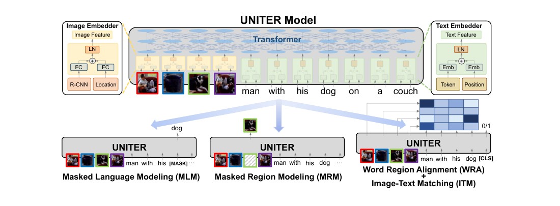
Figure 1: Overview of the proposed UNITER model (best viewed in color), consisting of an Image Embedder, a Text Embedder and a multi-layer Transformer, learned through four pre-training tasks
图 1:所提出的 UNITER 模型总览(建议看彩色图),由图像嵌入器、文本嵌入器和一个多层 Transformer 组成,并通过四项预训练任务来学习
As shown in Figure 1, UNITER first encodes image regions (visual features and bounding box features) and textual words (tokens and positions) into a common embedding space with Image Embedder and Text Embedder. Then, a Transformer module is applied to learn generalizable contextualized embeddings for each region and each word through well-designed pre-training tasks. Compared with previous work on multimodal pre-training [47, 29, 1, 24, 42, 60, 25]: () our masked language/region modeling is conditioned on full observation of image/text, rather than applying joint random masking to both modalities; () we introduce a novel WRA pre-training task via the use of Optimal Transport (OT) [37, 7] to explicitly encourage fine-grained alignment between words and image regions. Intuitively, OT-based learning aims to optimize for distribution matching via minimizing the cost of transporting one distribution to another. In our context, we aim to minimize the cost of transporting the embeddings from image regions to words in a sentence (and vice versa), thus optimizing towards better cross-modal alignment. We show that both conditional masking and OT-based WRA can successfully ease the misalignment between images and text, leading to better joint embeddings for downstream tasks.
如图 1 所示,UNITER 首先用图像嵌入器和文本嵌入器,把图像区域(视觉特征和边框特征)以及文本中的词(词元和位置)编码到一个共用的嵌入空间。随后,一个 Transformer 模块通过精心设计的预训练任务,为每个区域和每个词学习可推广的上下文嵌入。与先前的多模态预训练工作 [47, 29, 1, 24, 42, 60, 25] 相比:() 我们的掩码语言/区域建模是在完整观察到图像/文本的条件下进行的,而不是对两个模态一起做联合随机掩码;() 我们借助最优传输(OT) [37, 7] 提出一项新的 WRA 预训练任务,以显式地鼓励词与图像区域之间的细粒度对齐。直观上看,基于 OT 的学习旨在通过最小化把一个分布搬运到另一个分布的代价,来优化分布匹配。在我们的设定里,目标是最小化把图像区域嵌入搬运到句子中各个词的代价(以及反过来),从而朝着更好的跨模态对齐去优化。我们表明,条件掩码和基于 OT 的 WRA 都能有效缓解图像与文本之间的错位,从而为下游任务得到更好的联合嵌入。
To demonstrate the generalizable power of UNITER, we evaluate on six V+L tasks across nine datasets, including: () VQA; () Visual Commonsense Reasoning (VCR) [58]; () NLVR2 [44]; () Visual Entailment [52]; () Image-Text Retrieval (including zero-shot setting) [23]; and () Referring Expression Comprehension [56]. Our UNITER model is trained on a large-scale V+L dataset composed of four subsets: () COCO [26]; () Visual Genome (VG) [21]; () Conceptual Captions (CC) [41]; and () SBU Captions [32]. Experiments show that UNITER achieves new state of the art with significant performance boost across all nine downstream datasets. Moreover, training on additional CC and SBU data (containing unseen images/text in downstream tasks) further boosts model performance over training on COCO and VG only.
为了展示 UNITER 的泛化能力,我们在跨越九个数据集的六类 V+L 任务上做评估,包括:() VQA;() 视觉常识推理(VCR) [58];() NLVR2 [44];() 视觉蕴含 [52];() 图文检索(含零样本设定) [23];以及 () 指称理解 [56]。UNITER 的训练数据是由四个子集组成的大规模 V+L 数据集:() COCO [26];() Visual Genome(VG) [21];() Conceptual Captions(CC) [41];以及 () SBU Captions [32]。实验表明,UNITER 在全部九个下游数据集上都取得了新的最好成绩,并带来显著的性能提升。此外,在 COCO 和 VG 之外再加入 CC 和 SBU 数据(其中包含下游任务中未见过的图像/文本)训练,还能把仅在 COCO 和 VG 上训练的结果再往上推一截。
Our contributions are summarized as follows: () We introduce UNITER, a powerful UNiversal Image-TExt Representation for V+L tasks. () We present Conditional Masking for masked language/region modeling, and propose a novel Optimal-Transport-based Word-Region Alignment task for pre-training. () We achieve new state of the art on a wide range of V+L benchmarks, outperforming existing multimodal pre-training methods by a large margin. We also present extensive experiments and analysis to provide useful insights on the effectiveness of each pre-training task/dataset for multimodal encoder training.
我们的贡献概括如下:() 提出 UNITER,一种面向 V+L 任务、能力较强的通用图像-文本表征。() 为掩码语言/区域建模引入条件掩码,并提出一项基于最优传输的新型词-区域对齐预训练任务。() 在一系列 V+L 基准上取得新的最好成绩,大幅度超过已有的多模态预训练方法。我们还给出了大量实验与分析,以说明各项预训练任务/数据集对多模态编码器训练的作用。
2 Related Work
2 相关工作
Self-supervised learning utilizes original data as its own source of supervision, which has been applied to many Computer Vision tasks, such as image colorization [59], solving jigsaw puzzles [31, 48], inpainting [35], rotation prediction [15], and relative location prediction [10]. Recently, pre-trained language models, such as ELMo [36], BERT [9], GPT2 [39], XLNet [54], RoBERTa [27] and ALBERT [22], have pushed great advances for NLP tasks. There are two keys to their success: effective pre-training tasks over large language corpus, and the use of Transformer [49] for learning contextualized text representations.
自监督学习利用原始数据自身作为监督来源,已被用于许多计算机视觉任务,例如图像着色 [59]、拼图 [31, 48]、补全 [35]、旋转预测 [15] 以及相对位置预测 [10]。近来,预训练语言模型,如 ELMo [36]、BERT [9]、GPT2 [39]、XLNet [54]、RoBERTa [27] 和 ALBERT [22],为自然语言处理任务带来了显著进展。它们成功的两个关键是:在大规模语料上使用有效的预训练任务,以及用 Transformer [49] 学习上下文相关的文本表征。
More recently, there has been a surging interest in self-supervised learning for multimodal tasks, by pre-training on large-scale image/video and text pairs, then finetuning on downstream tasks. For example, VideoBERT [46] and CBT [45] applied BERT to learn a joint distribution over video frame features and linguistic tokens from video-text pairs. ViLBERT [29] and LXMERT [47] introduced the two-stream architecture, where two Transformers are applied to images and text independently, which is fused by a third Transformer in a later stage. On the other hand, B2T2 [1], VisualBERT [25], Unicoder-VL [24] and VL-BERT [42] proposed the single-stream architecture, where a single Transformer is applied to both images and text. VLP [60] applied pre-trained models to both image captioning and VQA. More recently, multi-task learning [30] and adversarial training [12] were used to further boost the performance. VALUE [6] developed a set of probing tasks to understand pre-trained models.
最近,把自监督学习用于多模态任务的兴趣迅速上升:先在大规模图像/视频与文本对上预训练,再在下游任务上微调。例如,VideoBERT [46] 和 CBT [45] 把 BERT 用到视频-文本对上,学习视频帧特征与语言词元的联合分布。ViLBERT [29] 和 LXMERT [47] 引入了双流结构,分别用两个 Transformer 独立处理图像和文本,再在较后阶段用第三个 Transformer 融合。另一方面,B2T2 [1]、VisualBERT [25]、Unicoder-VL [24] 和 VL-BERT [42] 提出了单流结构,用同一个 Transformer 同时处理图像和文本。VLP [60] 把预训练模型同时用于图像描述和 VQA。更近一些,多任务学习 [30] 和对抗训练 [12] 也被用来进一步提升性能。VALUE [6] 则设计了一组探针任务,用来理解预训练模型。
Our Contributions The key differences between our UNITER model and the other methods are two-fold: () UNITER uses conditional masking on MLM and MRM, i.e., masking only one modality while keeping the other untainted; and () a novel Word-Region Alignment pre-training task via the use of Optimal Transport, while in previous work such alignment is only implicitly enforced by task-specific losses. In addition, we examine the best combination of pre-training tasks through a thorough ablation study, and achieve new state of the art on multiple V+L datasets, often outperforming prior work by a large margin.
我们的贡献 UNITER 与其他方法的关键差异有两点:() UNITER 在 MLM 和 MRM 上使用条件掩码,也就是只掩码一个模态,同时保持另一个模态完整不变;以及 () 借助最优传输提出一项新的词-区域对齐预训练任务,而在先前工作中,这种对齐往往只由任务特定的损失隐式地施加。此外,我们通过细致的消融考察了预训练任务的最佳组合,并在多个 V+L 数据集上取得新的最好成绩,常常大幅度超过已有工作。
3 UNiversal Image-TExt Representation
3 通用图像-文本表征
In this section, we first introduce the model architecture of UNITER (Section 3.1), then describe the designed pre-training tasks and V+L datasets used for pre-training (Section 3.2 and 3.3).
本节先介绍 UNITER 的模型结构(第 3.1 节),再说明所设计的预训练任务以及用于预训练的 V+L 数据集(第 3.2 节和第 3.3 节)。
3.1 Model Overview
3.1 模型概览
The model architecture of UNITER is illustrated in Figure 1. Given a pair of image and sentence, UNITER takes the visual regions of the image and textual tokens of the sentence as inputs. We design an Image Embedder and a Text Embedder to extract their respective embeddings. These embeddings are then fed into a multi-layer Transformer to learn a cross-modality contextualized embedding across visual regions and textual tokens. Note that the self-attention mechanism in Transformer is order-less, thus it is necessary to explicitly encode the positions of tokens and the locations of regions as additional inputs.
UNITER 的模型结构如图 1 所示。给定一对图像和句子,UNITER 以图像的视觉区域和句子的文本词元作为输入。我们设计了图像嵌入器和文本嵌入器,分别提取两者的嵌入。这些嵌入再送入一个多层 Transformer,以学习跨越视觉区域与文本词元的跨模态上下文嵌入。需要注意的是,Transformer 中的自注意力机制是无序的,因此有必要把词元的位置以及区域的空间位置作为额外输入显式地编码进去。
Specifically, in Image Embedder, we first use Faster R-CNN[^2] to extract the visual features (pooled ROI features) for each region. We also encode the location features for each region via a 7-dimensional vector.[^3] Both visual and location features are then fed through a fully-connected (FC) layer, to be projected into the same embedding space. The final visual embedding for each region is obtained by summing up the two FC outputs and then passing through a layer normalization (LN) layer. For Text Embedder, we follow BERT [9] and tokenize the input sentence into WordPieces [51]. The final representation for each sub-word token[^4] is obtained via summing up its word embedding and position embedding, followed by another LN layer.[^5]
具体而言,在图像嵌入器中,我们首先用 Faster R-CNN[^2] 提取每个区域的视觉特征(汇聚后的 ROI 特征)。我们还用一个 7 维向量编码每个区域的位置特征。[^3] 视觉特征和位置特征再分别通过一层全连接(FC),投影到同一嵌入空间。每个区域的最终视觉嵌入,由两个 FC 输出相加后再经过一层层归一化(LN)得到。对文本嵌入器,我们沿用 BERT [9],把输入句子切成 WordPieces [51]。每个子词词元[^4] 的最终表示,由其词嵌入与位置嵌入相加,再经过另一层 LN 得到。[^5]
We introduce four main tasks to pre-train our model: Masked Language Modeling conditioned on image regions (MLM), Masked Region Modeling conditioned on input text (with three variants) (MRM), Image-Text Matching (ITM), and Word-Region Alignment (WRA). As shown in Figure 1, our MRM and MLM are in analogy to BERT, where we randomly mask some words or regions from the input and learn to recover the words or regions as the output of Transformer. Specifically, word masking is realized by replacing the token with a special token [MASK], and region masking is implemented by replacing the visual feature vector with all zeros. Note that each time we only mask one modality while keeping the other modality intact, instead of randomly masking both modalities as used in other pre-training methods. This prevents potential misalignment when a masked region happens to be described by a masked word (detailed in Section 4.2).
我们引入四项主要任务来预训练模型:以图像区域为条件的掩码语言建模(MLM)、以输入文本为条件的掩码区域建模(含三种变体)(MRM)、图文匹配(ITM),以及词-区域对齐(WRA)。如图 1 所示,我们的 MRM 和 MLM 与 BERT 类似:从输入中随机掩码一些词或区域,并学习在 Transformer 的输出中把这些词或区域还原回来。具体来说,词的掩码是把该词元替换成特殊词元 [MASK],区域掩码则是把视觉特征向量替换成全零。注意,每次我们只掩码一个模态,同时保持另一个模态完整,而不是像其他预训练方法那样对两个模态同时随机掩码。这样可以避免被掩码的区域恰好被一个也被掩码的词所描述时可能出现的错位(详见第 4.2 节)。
We also learn an instance-level alignment between the whole image and the sentence via ITM. During training, we sample both positive and negative image-sentence pairs and learn their matching scores. Furthermore, in order to provide a more fine-grained alignment between word tokens and image regions, we propose WRA via the use of Optimal Transport, which effectively calculates the minimum cost of transporting the contextualized image embeddings to word embeddings (and vice versa). The inferred transport plan thus serves as a propeller for better cross-modal alignment. Empirically, we show that both conditional masking and WRA contributes to performance improvement (in Section 4.2). To pre-train UNITER with these tasks, we randomly sample one task for each mini-batch, and train on only one objective per SGD update.
我们还通过 ITM 学习整幅图像与整句之间的实例级对齐。训练时,我们同时采样正、负图文句对,并学习它们的匹配分数。此外,为了在词元与图像区域之间提供更细粒度的对齐,我们提出借助最优传输的 WRA,它能有效计算把上下文相关的图像嵌入搬运到词嵌入(以及反过来)的最小代价。由此推断出的传输方案,便成为推动更好跨模态对齐的力量。经验上,我们表明条件掩码和 WRA 都有助于提升性能(见第 4.2 节)。在用这些任务预训练 UNITER 时,我们为每个小批量随机采样一项任务,并在每次 SGD 更新中只优化一个目标。
3.2 Pre-training Tasks
3.2 预训练任务
Masked Language Modeling (MLM) We denote the image regions as , the input words as , and the mask indices as .[^6] In MLM, we randomly mask out the input words with probability of 15%, and replace the masked ones with special token [MASK].[^7] The goal is to predict these masked words based on the observation of their surrounding words and all image regions , by minimizing the negative log-likelihood:
掩码语言建模(MLM) 我们将图像区域记为 ,输入词记为 ,掩码下标记为 。[^6] 在 MLM 中,我们以 15% 的概率随机掩码输入词,并把被掩码的词 替换成特殊词元 [MASK]。[^7] 目标是在观察到其上下文词 以及全部图像区域 的条件下,预测这些被掩码的词,并通过最小化负对数似然来学习:
where is the trainable parameters. Each pair is sampled from the whole training set .
其中 是可训练参数。每一对 从整个训练集 中采样。
Image-Text Matching (ITM) In ITM, an additional special token [CLS] is fed into our model, which indicates the fused representation of both modalities. The inputs to ITM are a sentence and a set of image regions, and the output is a binary label , indicating if the sampled pair is a match. We extract the representation of [CLS] token as the joint representation of the input image-text pair, then feed it into an FC layer and a sigmoid function to predict a score between 0 and 1. We denote the output score as . The ITM supervision is over the [CLS] token.[^8] During training, we sample a positive or negative pair from the dataset at each step. The negative pair is created by replacing the image or text in a paired sample with a randomly-selected one from other samples. We apply the binary cross-entropy loss for optimization:
图文匹配(ITM) 在 ITM 中,模型还会读入一个额外的特殊词元 [CLS],用来表示两个模态融合后的表征。ITM 的输入是一个句子和一组图像区域,输出是二值标签 ,表示采样到的这对是否匹配。我们提取 [CLS] 词元的表示作为输入图文对的联合表征,再送入一层 FC 和 sigmoid 函数,预测一个介于 0 和 1 之间的分数。将该输出分数记为 。ITM 的监督加在 [CLS] 词元上。[^8] 训练时,我们在每一步从数据集 中采样一个正对或负对 。负对的构造方式,是把一对匹配样本中的图像或文本,替换成从其他样本里随机选出的一个。我们用二元交叉熵损失来优化:
Word-Region Alignment (WRA) We use Optimal Transport (OT) for WRA, where a transport plan is learned to optimize the alignment between and . OT possesses several idiosyncratic characteristics that make it a good choice for WRA: () Self-normalization: all the elements of sum to 1 [37]. () Sparsity: when solved exactly, OT yields a sparse solution containing non-zero elements at most, where , leading to a more interpretable and robust alignment [37]. () Efficiency: compared with conventional linear programming solvers, our solution can be readily obtained using iterative procedures that only require matrix-vector products [53], hence readily applicable to large-scale model pre-training.
词-区域对齐(WRA) 我们把最优传输(OT)用于 WRA,学习一个传输方案 ,以优化 与 之间的对齐。OT 具有若干独特的性质,使它适合做 WRA:() 自归一化: 的所有元素之和为 1 [37]。() 稀疏性:在精确求解时,OT 会给出一个稀疏解 ,其中非零元素至多有 个,这里 ,从而得到更可解释、也更稳健的对齐 [37]。() 效率:与常规的线性规划求解器相比,我们的解可以用只需要矩阵-向量乘法的迭代过程得到 [53],因此很容易用于大规模模型预训练。
Specifically, can be considered as two discrete distributions , formulated as and , with as the Dirac function centered on . The weight vectors and belong to the - and -dimensional simplex, respectively (i.e., ), as both and are probability distributions. The OT distance between and (thus also the alignment loss for the () pair) is defined as:
具体而言, 可以被看作两个离散分布 ,写成 以及 ,其中 是中心在 上的 Dirac 函数。权重向量 和 分别属于 维和 维单纯形(也就是 ),因为 和 都是概率分布。 与 之间的 OT 距离(因而也是这对 的对齐损失)定义为:
where , denotes an -dimensional all-one vector, and is the cost function evaluating the distance between and . In experiments, the cosine distance is used. The matrix is denoted as the transport plan, interpreting the alignment between two modalities. Unfortunately, the exact minimization over is computational intractable, and we consider the IPOT algorithm [53] to approximate the OT distance (details are provided in the supplementary file). After solving , the OT distance serves as the WRA loss that can be used to update the parameters .
其中 , 表示 维全 1 向量, 是衡量 与 之间距离的代价函数。实验中使用余弦距离 。矩阵 被称为传输方案,用来解释两个模态之间的对齐。遗憾的是,对 的精确最小化在计算上难以完成,我们因此采用 IPOT 算法 [53] 来近似 OT 距离(细节见补充材料)。在求出 之后,OT 距离便作为可用于更新参数 的 WRA 损失。
Masked Region Modeling (MRM) Similar to MLM, we also sample image regions and mask their visual features with a probability of 15%. The model is trained to reconstruct the masked regions given the remaining regions and all the words . The visual features of the masked region are replaced by zeros. Unlike textual tokens that are represented as discrete labels, visual features are high-dimensional and continuous, thus cannot be supervised via class likelihood. Instead, we propose three variants for MRM, which share the same objective base:
掩码区域建模(MRM) 与 MLM 类似,我们也对图像区域采样,并以 15% 的概率掩码其视觉特征。模型被训练为:在给定剩余区域 以及全部词 的条件下,重建被掩码的区域 。被掩码区域的视觉特征用零向量替换。与被表示为离散标签的文本词元不同,视觉特征是高维且连续的,因而无法用类别似然来监督。于是我们为 MRM 提出三种变体,它们共享同一个目标形式:
- Masked Region Feature Regression (MRFR) MRFR learns to regress the Transformer output of each masked region to its visual features. Specifically, we apply an FC layer to convert its Transformer output into a vector of same dimension as the input ROI pooled feature . Then we apply L2 regression between the two: .
1)掩码区域特征回归(MRFR) MRFR 学习把每个被掩码区域 的 Transformer 输出回归到其视觉特征。具体来说,我们用一层 FC 把它的 Transformer 输出转换成与输入 ROI 汇聚特征 维数相同的向量 。然后对二者做 L2 回归:。
- Masked Region Classification (MRC) MRC learns to predict the object semantic class for each masked region. We first feed the Transformer output of the masked region into an FC layer to predict the scores of object classes, which further goes through a softmax function to be transformed into a normalized distribution . Note that there is no ground-truth label, as the object categories are not provided. Thus, we use the object detection output from Faster R-CNN, and take the detected object category (with the highest confidence score) as the label of the masked region, which will be converted into a one-hot vector . The final objective minimizes the cross-entropy (CE) loss: .
2)掩码区域分类(MRC) MRC 学习为每个被掩码区域预测物体的语义类别。我们先把被掩码区域 的 Transformer 输出送入一层 FC,预测 个物体类别的分数,再经 softmax 变成归一化分布 。需要注意的是,这里并没有真实标签,因为并未提供物体类别。于是我们使用 Faster R-CNN 的目标检测输出,把检测到的物体类别(置信度最高者)当作被掩码区域的标签,并转换成 one-hot 向量 。最终目标是最小化交叉熵(CE)损失:。
- Masked Region Classification with KL-Divergence (MRC-kl) MRC takes the most likely object class from the object detection model as the hard label (w.p. 0 or 1), assuming the detected object class is the ground-truth label for the region. However, this may not be true, as no ground-truth label is available. Thus, in MRC-kl, we avoid this assumption by using soft label as supervision signal, which is the raw output from the detector (i.e., a distribution of object classes ). MRC-kl aims to distill such knowledge into UNITER as [16], by minimizing the KL divergence between two distributions: .
3)带 KL 散度的掩码区域分类(MRC-kl) MRC 把检测模型给出的最可能物体类别当作硬标签(概率为 0 或 1),并假定检测到的类别就是该区域的真实标签。然而这并不一定成立,因为实际上并没有真实标签可用。因此在 MRC-kl 中,我们改用软标签作为监督信号,也就是检测器的原始输出(物体类别分布 ),从而避免这一假定。MRC-kl 的目标是把这类知识蒸馏进 UNITER,如 [16] 那样,通过最小化两个分布之间的 KL 散度:。
| In-domain | Out-of-domain | |||
|---|---|---|---|---|
| Split | COCO Captions | VG Dense Captions | Conceptual Captions | SBU Captions |
| train | 533K (106K) | 5.06M (101K) | 3.0M (3.0M) | 990K (990K) |
| val | 25K (5K) | 106K (2.1K) | 14K (14K) | 10K (10K) |
Table 1: Statistics on the datasets used for pre-training. Each cell shows #image-text pairs (#images)
| 域内 | 域内 | 域外 | 域外 | |
|---|---|---|---|---|
| 划分 | COCO Captions | VG Dense Captions | Conceptual Captions | SBU Captions |
| train | 533K(106K) | 5.06M(101K) | 3.0M(3.0M) | 990K(990K) |
| val | 25K(5K) | 106K(2.1K) | 14K(14K) | 10K(10K) |
表 1:预训练所用数据集的统计。每个单元格给出图文对数(图像数)
3.3 Pre-training Datasets
3.3 预训练数据集
We construct our pre-training dataset based on four existing V+L datasets: COCO [26], Visual Genome (VG) [21], Conceptual Captions (CC) [41], and SBU Captions [32]. Only image and sentence pairs are used for pre-training, which makes the model framework more scalable, as additional image-sentence pairs are easy to harvest for further pre-training.
我们基于已有的四份 V+L 数据集来构建预训练数据:COCO [26]、Visual Genome(VG) [21]、Conceptual Captions(CC) [41] 以及 SBU Captions [32]。预训练只用图像和句子对,这使模型框架更易于扩展,因为要为进一步预训练收集额外的图文句对并不困难。
To study the effects of different datasets on pre-training, we divide the four datasets into two categories. The first one consists of image captioning data from COCO and dense captioning data from VG. We call it “In-domain” data, as most V+L tasks are built on top of these two datasets. To obtain a “fair” data split, we merge the raw training and validation splits from COCO, and exclude all validation and test images that appear in downstream tasks. We also exclude all co-occurring Flickr30K [38] images via URL matching, as both COCO and Flickr30K images were crawled from Flickr and may have overlaps.[^9] The same rule was applied to Visual Genome as well. In this way, we obtain 5.6M image-text pairs for training and 131K image-text pairs for our internal validation, which is half the size of the dataset used in LXMERT [47], due to the filtering of overlapping images and the use of image-text pairs only. We also use additional Out-of-domain data from Conceptual Captions [41] and SBU Captions [32] for model training.[^10] The statistics on the cleaned splits are provided in Table 1.
为了考察不同数据集对预训练的影响,我们把这四份数据分成两类。第一类由 COCO 的图像描述数据和 VG 的稠密描述数据组成。我们称之为“域内”数据,因为大多数 V+L 任务都建立在这两份数据集之上。为了得到一个“公平”的数据划分,我们合并 COCO 原始的训练与验证划分,并排除所有出现在下游任务中的验证和测试图像。我们还通过 URL 匹配排除了所有同时出现的 Flickr30K [38] 图像,因为 COCO 和 Flickr30K 的图像都是从 Flickr 抓取的,可能存在重叠。[^9] 同样的规则也应用于 Visual Genome。这样,我们得到 560 万个图文对用于训练,以及 13.1 万个图文对用于内部验证;由于过滤了重叠图像并且只使用图文对,其规模约为 LXMERT [47] 所用数据集的一半。我们还使用来自 Conceptual Captions [41] 和 SBU Captions [32] 的额外域外数据来训练模型。[^10] 清理后各划分的统计见表 1。
4 Experiments
4 实验
We evaluate UNITER on six V+L tasks[^11] by transferring the pre-trained model to each target task and finetuning through end-to-end training. We report experimental results on two model sizes: UNITER-base with 12 layers and UNITER-large with 24 layers.[^12]
我们通过把预训练模型迁移到各个目标任务、并做端到端微调,在六类 V+L 任务[^11] 上评估 UNITER。我们报告两种模型规模的实验结果:12 层的 UNITER-base,以及 24 层的 UNITER-large。[^12]
| Pre-training Data | Pre-training Tasks | Meta-Sum | VQA test-dev | IR (Flickr) val | TR (Flickr) val | NLVR2 dev | RefCOCO+ vald |
|---|---|---|---|---|---|---|---|
| None | None | 314.34 | 67.03 | 61.74 | 65.55 | 51.02 | 68.73 |
| Wikipedia + BookCorpus | MLM (text only) | 346.24 | 69.39 | 73.92 | 83.27 | 50.86 | 68.80 |
| In-domain (COCO+VG) | MRFR | 344.66 | 69.02 | 72.10 | 82.91 | 52.16 | 68.47 |
| In-domain (COCO+VG) | ITM | 385.29 | 70.04 | 78.93 | 89.91 | 74.08 | 72.33 |
| In-domain (COCO+VG) | MLM | 386.10 | 71.29 | 77.88 | 89.25 | 74.79 | 72.89 |
| In-domain (COCO+VG) | MLM + ITM | 393.04 | 71.55 | 81.64 | 91.12 | 75.98 | 72.75 |
| In-domain (COCO+VG) | MLM + ITM + MRC | 393.97 | 71.46 | 81.39 | 91.45 | 76.18 | 73.49 |
| In-domain (COCO+VG) | MLM + ITM + MRFR | 396.24 | 71.73 | 81.76 | 92.31 | 76.21 | 74.23 |
| In-domain (COCO+VG) | MLM + ITM + MRC-kl | 397.09 | 71.63 | 82.10 | 92.57 | 76.28 | 74.51 |
| In-domain (COCO+VG) | MLM + ITM + MRC-kl + MRFR | 399.97 | 71.92 | 83.73 | 92.87 | 76.93 | 74.52 |
| In-domain (COCO+VG) | MLM + ITM + MRC-kl + MRFR + WRA | 400.93 | 72.47 | 83.72 | 93.03 | 76.91 | 74.80 |
| In-domain (COCO+VG) | MLM + ITM + MRC-kl + MRFR (w/o cond. mask) | 396.51 | 71.68 | 82.31 | 92.08 | 76.15 | 74.29 |
| Out-of-domain (SBU+CC) | MLM + ITM + MRC-kl + MRFR + WRA | 396.91 | 71.56 | 84.34 | 92.57 | 75.66 | 72.78 |
| In-domain + Out-of-domain | MLM + ITM + MRC-kl + MRFR + WRA | 405.24 | 72.70 | 85.77 | 94.28 | 77.18 | 75.31 |
Table 2: Evaluation on pre-training tasks and datasets using VQA, Image-Text Retrieval on Flickr30K, NLVR2, and RefCOCO+ as benchmarks. All results are from UNITER-base. Averages of R@1, R@5 and R@10 on Flickr30K for Image Retrieval (IR) and Text Retrieval (TR) are reported. Dark and light grey colors highlight the top and second best results across all the tasks trained with In-domain data
| 预训练数据 | 预训练任务 | Meta-Sum | VQA test-dev | IR(Flickr)val | TR(Flickr)val | NLVR2 dev | RefCOCO+ vald |
|---|---|---|---|---|---|---|---|
| 无 | 无 | 314.34 | 67.03 | 61.74 | 65.55 | 51.02 | 68.73 |
| Wikipedia + BookCorpus | 仅文本 MLM | 346.24 | 69.39 | 73.92 | 83.27 | 50.86 | 68.80 |
| 域内(COCO+VG) | MRFR | 344.66 | 69.02 | 72.10 | 82.91 | 52.16 | 68.47 |
| 域内(COCO+VG) | ITM | 385.29 | 70.04 | 78.93 | 89.91 | 74.08 | 72.33 |
| 域内(COCO+VG) | MLM | 386.10 | 71.29 | 77.88 | 89.25 | 74.79 | 72.89 |
| 域内(COCO+VG) | MLM + ITM | 393.04 | 71.55 | 81.64 | 91.12 | 75.98 | 72.75 |
| 域内(COCO+VG) | MLM + ITM + MRC | 393.97 | 71.46 | 81.39 | 91.45 | 76.18 | 73.49 |
| 域内(COCO+VG) | MLM + ITM + MRFR | 396.24 | 71.73 | 81.76 | 92.31 | 76.21 | 74.23 |
| 域内(COCO+VG) | MLM + ITM + MRC-kl | 397.09 | 71.63 | 82.10 | 92.57 | 76.28 | 74.51 |
| 域内(COCO+VG) | MLM + ITM + MRC-kl + MRFR | 399.97 | 71.92 | 83.73 | 92.87 | 76.93 | 74.52 |
| 域内(COCO+VG) | MLM + ITM + MRC-kl + MRFR + WRA | 400.93 | 72.47 | 83.72 | 93.03 | 76.91 | 74.80 |
| 域内(COCO+VG) | MLM + ITM + MRC-kl + MRFR(无条件掩码) | 396.51 | 71.68 | 82.31 | 92.08 | 76.15 | 74.29 |
| 域外(SBU+CC) | MLM + ITM + MRC-kl + MRFR + WRA | 396.91 | 71.56 | 84.34 | 92.57 | 75.66 | 72.78 |
| 域内 + 域外 | MLM + ITM + MRC-kl + MRFR + WRA | 405.24 | 72.70 | 85.77 | 94.28 | 77.18 | 75.31 |
表 2:以 VQA、Flickr30K 上的图文检索、NLVR2 和 RefCOCO+ 为基准,评估预训练任务与数据集。全部结果来自 UNITER-base。Flickr30K 上的图像检索(IR)和文本检索(TR)报告 R@1、R@5 与 R@10 的平均值。深灰与浅灰色分别标出在域内数据上训练的各项任务中最好和次好的结果
4.1 Downstream Tasks
4.1 下游任务
In VQA, VCR and NLVR2 tasks, given an input image (or a pair of images) and a natural language question (or description), the model predicts an answer (or judges the correctness of the description) based on the visual content in the image. For Visual Entailment, we evaluate on the SNLI-VE dataset. The goal is to predict whether a given image semantically entails an input sentence. Classification accuracy over three classes (‘‘Entailment”, ‘‘Neutral” and ‘‘Contradiction”) is used to measure model performance. For Image-Text Retrieval, we consider two datasets (COCO and Flickr30K) and evaluate the model in two settings: Image Retrieval (IR) and Text Retrieval (TR). Referring Expression (RE) Comprehension requires the model to select the target from a set of image region proposals given the query description. Models are evaluated on both ground-truth objects and detected proposals[^13] (MAttNet [55]).
在 VQA、VCR 和 NLVR2 任务中,给定一张输入图像(或一对图像)以及一个自然语言问题(或描述),模型根据图像中的视觉内容预测答案(或判断该描述是否正确)。对视觉蕴含,我们在 SNLI-VE 数据集上评估。目标是预测给定图像是否在语义上蕴含输入句子。用三个类别(“蕴含”“中立”和“矛盾”)上的分类准确率来衡量模型表现。对图文检索,我们考虑两份数据集(COCO 和 Flickr30K),并在两种设定下评估模型:图像检索(IR)和文本检索(TR)。指称理解(RE)要求模型在给定查询描述的情况下,从一组图像区域提议中选出目标。模型同时在真实物体和检测出的提议[^13] 上评估(MAttNet [55])。
For VQA, VCR, NLVR2, Visual Entailment and Image-Text Retrieval, we extract the joint embedding of the input image-text pairs via a multi-layer perceptron (MLP) from the representation of the [CLS] token. For RE Comprehension, we use the MLP to compute the region-wise alignment scores. These MLP layers are learned during the finetuning stage. Specifically, we formulate VQA, VCR, NLVR2, Visual Entailment and RE Comprehension as classification problems and minimize the cross-entropy over the ground-truth answers/responses. For Image-Text Retrieval, we formulate it as a ranking problem. During finetuning, we sample three pairs of image and text, one positive pair from the dataset and two negative pairs by randomly replacing its sentence/image with others. We compute the similarity scores (based on the joint embedding) for both positive and negative pairs, and maximize the margin between them through triplet loss.
对 VQA、VCR、NLVR2、视觉蕴含和图文检索,我们从 [CLS] 词元的表示出发,用一个多层感知机(MLP)提取输入图文对的联合嵌入。对指称理解,我们用 MLP 计算区域级的对齐分数。这些 MLP 层在微调阶段学习。具体来说,我们把 VQA、VCR、NLVR2、视觉蕴含和指称理解写成分类问题,并最小化真实答案/回复上的交叉熵。对图文检索,我们把它写成排序问题。微调时,我们采样三对图文:一对来自数据集的正对,以及通过随机替换其句子/图像得到的两对负对。我们(基于联合嵌入)计算正对和负对的相似度分数,并通过三元组损失拉大正负对之间的间隔。
4.2 Evaluation on Pre-training Tasks
4.2 对预训练任务的评估
We analyze the effectiveness of different pre-training settings through ablation studies over VQA, NLVR2, Flickr30K and RefCOCO+ as representative V+L benchmarks. In addition to standard metrics[^14] for each benchmark , we also use Meta-Sum (sum of all the scores across all the benchmarks) as a global metric.
我们以 VQA、NLVR2、Flickr30K 和 RefCOCO+ 作为有代表性的 V+L 基准,通过消融来分析不同预训练设定的效果。除了各基准的标准指标[^14] 之外,我们还使用 Meta-Sum(所有基准上所有分数之和)作为总体指标。
Firstly, we establish two baselines: Line 1 (L1) in Table 2 indicates no pre-training is involved, and L2 shows the results from MLM initialized with pre-trained weights from [9]. Although MLM trained on text only did not absorb any image information during pre-training, we see a gain of approximately +30 on Meta-Sum over L1. Hence, we use the pre-trained weights in L2 to initialize our model for the following experiments.
首先,我们建立两条基线:表 2 中的第 1 行(L1)表示不做任何预训练,L2 给出用 [9] 的预训练权重初始化、只做 MLM 的结果。尽管只在文本上训练的 MLM 在预训练期间没有吸收任何图像信息,我们仍看到相对 L1,Meta-Sum 大约提升了 +30。因此,在后续实验中,我们用 L2 中的预训练权重来初始化模型。
Secondly, we validate the effectiveness of each pre-training task through a thorough ablation study. Comparing L2 and L3, MRFR (L3) achieves better results than MLM (L2) only on NLVR2. On the other hand, when pre-trained on ITM (L4) or MLM (L5) only, we observe a significant improvement across all the tasks over L1 and L2 baselines. When combining different pre-training tasks, MLM + ITM (L6) improves over single ITM (L4) or MLM (L5). When MLM, ITM and MRM are jointly trained (L7-L10), we observe consistent performance gain across all the benchmarks. Among the three variants of MRM (L7-L9), we observe that MRC-kl (L9) achieves the best performance (397.09) when combined with MLM + ITM, while MRC (L7) the worst (393.97). When combining MRC-kl and MRFR together with MLM and ITM (L10), we find that they are complimentary to each other, which leads to the second highest Meta-Sum score. The highest Meta-Sum Score is achieved by MLM + ITM + MRC-kl + MRFR + WRA (L11). We observe significant performance improvements from adding WRA, especially on VQA and RefCOCO+. It indicates the fine-grained alignment between words and regions learned through WRA during pre-training benefits the downstream tasks involving region-level recognition or reasoning. We use this optimal pre-training setting for the further experiments.
其次,我们通过细致的消融来验证各项预训练任务的作用。比较 L2 和 L3,MRFR(L3)只在 NLVR2 上比 MLM(L2)更好。另一方面,只在 ITM(L4)或只在 MLM(L5)上预训练时,我们在所有任务上都观察到相对 L1 和 L2 基线的显著提升。把不同预训练任务组合起来时,MLM + ITM(L6)优于单独的 ITM(L4)或 MLM(L5)。当 MLM、ITM 和 MRM 一起训练时(L7–L10),我们在全部基准上都观察到稳定的性能提升。在 MRM 的三种变体中(L7–L9),与 MLM + ITM 组合时,MRC-kl(L9)取得最好成绩(397.09),MRC(L7)最差(393.97)。把 MRC-kl 和 MRFR 与 MLM、ITM 一起组合(L10)时,我们发现它们彼此互补,得到次高的 Meta-Sum 分数。最高的 Meta-Sum 由 MLM + ITM + MRC-kl + MRFR + WRA(L11)取得。加入 WRA 后,我们观察到显著的性能提升,尤其是在 VQA 和 RefCOCO+ 上。这表明预训练期间通过 WRA 学到的词与区域之间的细粒度对齐,有益于涉及区域级识别或推理的下游任务。后续实验都采用这一最优预训练设定。
Additionally, we validate the contributions of conditional masking through a comparison study. When we perform random masking on both modalities simultaneously during pre-training, i.e., w/o conditional masking (L12), we observe a decrease in Meta-Sum score (396.51) compared to that with conditional masking (399.97). This indicates that the conditional masking strategy enables the model to learn better joint image-text representations effectively.
此外,我们通过对照实验验证条件掩码的贡献。当预训练时对两个模态同时做随机掩码,也就是不使用条件掩码(L12)时,我们观察到 Meta-Sum 分数(396.51)低于使用条件掩码时的结果(399.97)。这表明条件掩码策略能有效帮助模型学到更好的联合图文表征。
Lastly, we study the effects of pre-training datasets. Our experiments so far have been focused on In-domain data. In this study, we pre-train our model on Out-of-domain data (Conceptual Captions + SBU Captions). A performance drop (396.91 in L13) from the model trained on In-domain data (COCO + Visual Genome) (400.93 in L11) shows that although Out-of-domain data contain more images, the model still benefits more from being exposed to similar downstream images during pre-training. We further pre-train our model on both In-domain and Out-of-domain data. With doubled data size, the model continues to improve (405.24 in L14).
最后,我们考察预训练数据集的影响。到目前为止,实验都集中在域内数据上。在这项研究中,我们在域外数据(Conceptual Captions + SBU Captions)上预训练模型。与在域内数据(COCO + Visual Genome)上训练的模型(L11 中的 400.93)相比,性能下降(L13 中的 396.91)表明:尽管域外数据包含更多图像,模型仍更多地受益于在预训练中见到与下游相似的图像。我们进一步在域内加域外数据上同时预训练。数据规模翻倍后,模型继续提升(L14 中的 405.24)。
| Tasks | Split | SOTA | ViLBERT | VLBERT | Unicoder-VL | VisualBERT | LXMERT | UNITER-base | UNITER-large |
|---|---|---|---|---|---|---|---|---|---|
| VQA | test-dev | 70.63 | 70.55 | 71.79 | - | 70.80 | 72.42 | 72.70 | 73.82 |
| VQA | test-std | 70.90 | 70.92 | 72.22 | - | 71.00 | 72.54 | 72.91 | 74.02 |
| VCR | QA | 72.60 | 73.30 | 75.80 | - | 71.60 | - | 75.00 | 77.30 |
| VCR | QAR | 75.70 | 74.60 | 78.40 | - | 73.20 | - | 77.20 | 80.80 |
| VCR | QAR | 55.00 | 54.80 | 59.70 | - | 52.40 | - | 58.20 | 62.80 |
| NLVR2 | dev | 54.80 | - | - | - | 67.40 | 74.90 | 77.18 | 79.12 |
| NLVR2 | test-P | 53.50 | - | - | - | 67.00 | 74.50 | 77.85 | 79.98 |
| SNLI-VE | val | 71.56 | - | - | - | - | - | 78.59 | 79.39 |
| SNLI-VE | test | 71.16 | - | - | - | - | - | 78.28 | 79.38 |
| ZS IR (Flickr) | R@1 | - | 31.86 | - | 48.40 | - | - | 66.16 | 68.74 |
| ZS IR (Flickr) | R@5 | - | 61.12 | - | 76.00 | - | - | 88.40 | 89.20 |
| ZS IR (Flickr) | R@10 | - | 72.80 | - | 85.20 | - | - | 92.94 | 93.86 |
| IR (Flickr) | R@1 | 48.60 | 58.20 | - | 71.50 | - | - | 72.52 | 75.56 |
| IR (Flickr) | R@5 | 77.70 | 84.90 | - | 91.20 | - | - | 92.36 | 94.08 |
| IR (Flickr) | R@10 | 85.20 | 91.52 | - | 95.20 | - | - | 96.08 | 96.76 |
| IR (COCO) | R@1 | 38.60 | - | - | 48.40 | - | - | 50.33 | 52.93 |
| IR (COCO) | R@5 | 69.30 | - | - | 76.70 | - | - | 78.52 | 79.93 |
| IR (COCO) | R@10 | 80.40 | - | - | 85.90 | - | - | 87.16 | 87.95 |
| ZS TR (Flickr) | R@1 | - | - | - | 64.30 | - | - | 80.70 | 83.60 |
| ZS TR (Flickr) | R@5 | - | - | - | 85.80 | - | - | 95.70 | 95.70 |
| ZS TR (Flickr) | R@10 | - | - | - | 92.30 | - | - | 98.00 | 97.70 |
| TR (Flickr) | R@1 | 67.90 | - | - | 86.20 | - | - | 85.90 | 87.30 |
| TR (Flickr) | R@5 | 90.30 | - | - | 96.30 | - | - | 97.10 | 98.00 |
| TR (Flickr) | R@10 | 95.80 | - | - | 99.00 | - | - | 98.80 | 99.20 |
| TR (COCO) | R@1 | 50.40 | - | - | 62.30 | - | - | 64.40 | 65.68 |
| TR (COCO) | R@5 | 82.20 | - | - | 87.10 | - | - | 87.40 | 88.56 |
| TR (COCO) | R@10 | 90.00 | - | - | 92.80 | - | - | 93.08 | 93.76 |
| RefCOCO | val | 87.51 | - | - | - | - | - | 91.64 | 91.84 |
| RefCOCO | testA | 89.02 | - | - | - | - | - | 92.26 | 92.65 |
| RefCOCO | testB | 87.05 | - | - | - | - | - | 90.46 | 91.19 |
| RefCOCO | vald | 77.48 | - | - | - | - | - | 81.24 | 81.41 |
| RefCOCO | testAd | 83.37 | - | - | - | - | - | 86.48 | 87.04 |
| RefCOCO | testBd | 70.32 | - | - | - | - | - | 73.94 | 74.17 |
| RefCOCO+ | val | 75.38 | - | 80.31 | - | - | - | 83.66 | 84.25 |
| RefCOCO+ | testA | 80.04 | - | 83.62 | - | - | - | 86.19 | 86.34 |
| RefCOCO+ | testB | 69.30 | - | 75.45 | - | - | - | 78.89 | 79.75 |
| RefCOCO+ | vald | 68.19 | 72.34 | 72.59 | - | - | - | 75.31 | 75.90 |
| RefCOCO+ | testAd | 75.97 | 78.52 | 78.57 | - | - | - | 81.30 | 81.45 |
| RefCOCO+ | testBd | 57.52 | 62.61 | 62.30 | - | - | - | 65.58 | 66.70 |
| RefCOCOg | val | 81.76 | - | - | - | - | - | 86.52 | 87.85 |
| RefCOCOg | test | 81.75 | - | - | - | - | - | 86.52 | 87.73 |
| RefCOCOg | vald | 68.22 | - | - | - | - | - | 74.31 | 74.86 |
| RefCOCOg | testd | 69.46 | - | - | - | - | - | 74.51 | 75.77 |
Table 3: Results on downstream V+L tasks from UNITER, compared with task-specific state-of-the-art (SOTA) and previous pre-trained models. ZS: Zero-Shot, IR: Image Retrieval and TR: Text Retrieval
| 任务 | 划分 | SOTA | ViLBERT | VLBERT | Unicoder-VL | VisualBERT | LXMERT | UNITER-base | UNITER-large |
|---|---|---|---|---|---|---|---|---|---|
| VQA | test-dev | 70.63 | 70.55 | 71.79 | - | 70.80 | 72.42 | 72.70 | 73.82 |
| VQA | test-std | 70.90 | 70.92 | 72.22 | - | 71.00 | 72.54 | 72.91 | 74.02 |
| VCR | QA | 72.60 | 73.30 | 75.80 | - | 71.60 | - | 75.00 | 77.30 |
| VCR | QAR | 75.70 | 74.60 | 78.40 | - | 73.20 | - | 77.20 | 80.80 |
| VCR | QAR | 55.00 | 54.80 | 59.70 | - | 52.40 | - | 58.20 | 62.80 |
| NLVR2 | dev | 54.80 | - | - | - | 67.40 | 74.90 | 77.18 | 79.12 |
| NLVR2 | test-P | 53.50 | - | - | - | 67.00 | 74.50 | 77.85 | 79.98 |
| SNLI-VE | val | 71.56 | - | - | - | - | - | 78.59 | 79.39 |
| SNLI-VE | test | 71.16 | - | - | - | - | - | 78.28 | 79.38 |
| ZS IR (Flickr) | R@1 | - | 31.86 | - | 48.40 | - | - | 66.16 | 68.74 |
| ZS IR (Flickr) | R@5 | - | 61.12 | - | 76.00 | - | - | 88.40 | 89.20 |
| ZS IR (Flickr) | R@10 | - | 72.80 | - | 85.20 | - | - | 92.94 | 93.86 |
| IR (Flickr) | R@1 | 48.60 | 58.20 | - | 71.50 | - | - | 72.52 | 75.56 |
| IR (Flickr) | R@5 | 77.70 | 84.90 | - | 91.20 | - | - | 92.36 | 94.08 |
| IR (Flickr) | R@10 | 85.20 | 91.52 | - | 95.20 | - | - | 96.08 | 96.76 |
| IR (COCO) | R@1 | 38.60 | - | - | 48.40 | - | - | 50.33 | 52.93 |
| IR (COCO) | R@5 | 69.30 | - | - | 76.70 | - | - | 78.52 | 79.93 |
| IR (COCO) | R@10 | 80.40 | - | - | 85.90 | - | - | 87.16 | 87.95 |
| ZS TR (Flickr) | R@1 | - | - | - | 64.30 | - | - | 80.70 | 83.60 |
| ZS TR (Flickr) | R@5 | - | - | - | 85.80 | - | - | 95.70 | 95.70 |
| ZS TR (Flickr) | R@10 | - | - | - | 92.30 | - | - | 98.00 | 97.70 |
| TR (Flickr) | R@1 | 67.90 | - | - | 86.20 | - | - | 85.90 | 87.30 |
| TR (Flickr) | R@5 | 90.30 | - | - | 96.30 | - | - | 97.10 | 98.00 |
| TR (Flickr) | R@10 | 95.80 | - | - | 99.00 | - | - | 98.80 | 99.20 |
| TR (COCO) | R@1 | 50.40 | - | - | 62.30 | - | - | 64.40 | 65.68 |
| TR (COCO) | R@5 | 82.20 | - | - | 87.10 | - | - | 87.40 | 88.56 |
| TR (COCO) | R@10 | 90.00 | - | - | 92.80 | - | - | 93.08 | 93.76 |
| RefCOCO | val | 87.51 | - | - | - | - | - | 91.64 | 91.84 |
| RefCOCO | testA | 89.02 | - | - | - | - | - | 92.26 | 92.65 |
| RefCOCO | testB | 87.05 | - | - | - | - | - | 90.46 | 91.19 |
| RefCOCO | vald | 77.48 | - | - | - | - | - | 81.24 | 81.41 |
| RefCOCO | testAd | 83.37 | - | - | - | - | - | 86.48 | 87.04 |
| RefCOCO | testBd | 70.32 | - | - | - | - | - | 73.94 | 74.17 |
| RefCOCO+ | val | 75.38 | - | 80.31 | - | - | - | 83.66 | 84.25 |
| RefCOCO+ | testA | 80.04 | - | 83.62 | - | - | - | 86.19 | 86.34 |
| RefCOCO+ | testB | 69.30 | - | 75.45 | - | - | - | 78.89 | 79.75 |
| RefCOCO+ | vald | 68.19 | 72.34 | 72.59 | - | - | - | 75.31 | 75.90 |
| RefCOCO+ | testAd | 75.97 | 78.52 | 78.57 | - | - | - | 81.30 | 81.45 |
| RefCOCO+ | testBd | 57.52 | 62.61 | 62.30 | - | - | - | 65.58 | 66.70 |
| RefCOCOg | val | 81.76 | - | - | - | - | - | 86.52 | 87.85 |
| RefCOCOg | test | 81.75 | - | - | - | - | - | 86.52 | 87.73 |
| RefCOCOg | vald | 68.22 | - | - | - | - | - | 74.31 | 74.86 |
| RefCOCOg | testd | 69.46 | - | - | - | - | - | 74.51 | 75.77 |
表 3:UNITER 在下游 V+L 任务上的结果,并与任务特定的当时最好成绩(SOTA)以及先前的预训练模型比较。ZS:零样本,IR:图像检索,TR:文本检索
4.3 Results on Downstream Tasks
4.3 下游任务结果
Table 3 presents the results of UNITER on all downstream tasks. Both our base and large models are pre-trained on In-domain+Out-of-domain datasets, with the optimal pre-training setting: MLM+ITM+MRC-kl+MRFR+WRA. The implementation details of each task are provided in the supplementary file. We compare with both task-specific models and other pre-trained models on each downstream task. SOTA task-specific models include: MCAN [57] for VQA, MaxEnt [44] for NLVR2, B2T2 [1] for VCR, SCAN [23] for Image-Text Retrieval, EVE-Image [52] for SNLI-VE, and MAttNet for RE Comprehension (RefCOCO, RefCOCO+ and RefCOCOg).[^15] Other pre-trained models include: ViLBERT [29], LXMERT [47], Unicoder-VL [24], VisualBERT [25] and VLBERT [42].
表 3 给出了 UNITER 在全部下游任务上的结果。我们的 base 和 large 模型都在域内加域外数据集上,按最优预训练设定 MLM+ITM+MRC-kl+MRFR+WRA 进行预训练。各任务的实现细节见补充材料。我们在每个下游任务上同时与任务特定模型以及其他预训练模型比较。任务特定的 SOTA 模型包括:用于 VQA 的 MCAN [57]、用于 NLVR2 的 MaxEnt [44]、用于 VCR 的 B2T2 [1]、用于图文检索的 SCAN [23]、用于 SNLI-VE 的 EVE-Image [52],以及用于指称理解(RefCOCO、RefCOCO+ 和 RefCOCOg)的 MAttNet。[^15] 其他预训练模型包括:ViLBERT [29]、LXMERT [47]、Unicoder-VL [24]、VisualBERT [25] 和 VLBERT [42]。
Results show that our UNITER-large model achieves new state of the art across all the benchmarks. UNITER-base model also outperforms the others by a large margin across all tasks except VQA. Specifically, our UNITER-base model outperforms SOTA by approximately for VCR on QAR, for NLVR2, for SNLI-VE, on R@1 for Image-Text Retrieval ( for zero-shot setting), and for RE Comprehension.
结果表明,我们的 UNITER-large 模型在全部基准上都取得了新的最好成绩。UNITER-base 模型除 VQA 外,也在所有任务上大幅度超过其他方法。具体来说,UNITER-base 相对 SOTA 大约高出:VCR 的 QAR ,NLVR2 ,SNLI-VE ,图文检索的 R@1 (零样本设定下 ),以及指称理解 。
Note that LXMERT pre-trains with downstream VQA (+VG+GQA) data, which may help adapt the model to VQA task. However, when evaluated on unseen tasks such as NLVR2, UNITER-base achieves 3% gain over LXMERT. In addition, among all the models pre-trained on image-text pairs only, our UNITER-base outperforms the others by > on VQA.
需要注意的是,LXMERT 在预训练中使用了下游的 VQA(+VG+GQA)数据,这可能有助于模型适应 VQA 任务。不过,在 NLVR2 这类未见过的任务上评估时,UNITER-base 相对 LXMERT 仍有 3% 的提升。此外,在所有只在图文对上预训练的模型中,我们的 UNITER-base 在 VQA 上超过其他模型超过 。
It is also worth mentioning that both VilBERT and LXMERT observed two-stream model outperforms single-stream model, while our results show empirically that with our pre-training setting, single-stream model can achieve new state-of-the-art results, with much fewer parameters (UNITER-base: 86M, LXMERT: 183M, VilBERT: 221M).[^16]
同样值得一提的是,ViLBERT 和 LXMERT 都观察到双流模型优于单流模型,而我们的结果从经验上表明:在我们的预训练设定下,单流模型也可以取得新的最好成绩,并且参数量少得多(UNITER-base:8600 万,LXMERT:1.83 亿,ViLBERT:2.21 亿)。[^16]
| Stage I | Stage II | QA | QAR | QAR |
|---|---|---|---|---|
| N | N | 72.44 | 73.71 | 53.52 |
| N | Y | 73.52 | 75.34 | 55.6 |
| Y | N | 72.83 | 75.25 | 54.94 |
| Y | Y | 74.56 | 77.03 | 57.76 |
Table 4: Experiments on two-stage pre-training for VCR. Results are from UNITER-base on VCR val split. Stage I and Stage II denote first-stage and second-stage pre-training
| Setting | dev | test-P |
|---|---|---|
| Triplet | 73.03 | 73.89 |
| Pair | 75.85 | 75.80 |
| Pair-biattn | 77.18 | 77.85 |
Table 5: Experiments on three modified settings for NLVR2. All models use pre-trained UNITER-base
| 第一阶段 | 第二阶段 | QA | QAR | QAR |
|---|---|---|---|---|
| 否 | 否 | 72.44 | 73.71 | 53.52 |
| 否 | 是 | 73.52 | 75.34 | 55.6 |
| 是 | 否 | 72.83 | 75.25 | 54.94 |
| 是 | 是 | 74.56 | 77.03 | 57.76 |
表 4:VCR 两阶段预训练实验。结果来自 UNITER-base 在 VCR 验证集上的表现。Stage I 和 Stage II 分别表示第一阶段与第二阶段预训练
| 设定 | dev | test-P |
|---|---|---|
| Triplet | 73.03 | 73.89 |
| Pair | 75.85 | 75.80 |
| Pair-biattn | 77.18 | 77.85 |
表 5:NLVR2 上三种改动设定的实验。所有模型都使用预训练的 UNITER-base
For VCR, we propose a two-stage pre-training approach: () pre-train on standard pre-training datasets; and then () pre-train on downstream VCR dataset. Interestingly, while VLBERT and B2T2 observed that pre-training is not very helpful on VCR, we find that the second-stage pre-training can significantly boost model performance, while the first-stage pre-training still helps but with limited effects (results shown in Table 5). This indicates that the proposed two-stage approach is highly effective in our pre-trained model over new data that are unseen in pre-training datasets.
对 VCR,我们提出一种两阶段预训练方法:() 先在标准预训练数据集上预训练;然后 () 在下游 VCR 数据集上继续预训练。有意思的是,虽然 VLBERT 和 B2T2 观察到预训练对 VCR 帮助不大,我们发现第二阶段预训练能显著提升模型性能,而第一阶段预训练仍然有帮助,只是效果有限(结果见表 5)。这表明,所提出的两阶段方法,能有效地把我们的预训练模型用到预训练数据中未见过的新数据上。
Different from other tasks, NLVR2 takes two images as input. Thus, directly finetuning UNITER pre-trained with image-sentence pairs might not lead to optimal performance, as the interactions between paired images are not learned during the pre-training stage. Thus, we experimented with three modified settings on NLVR2: () Triplet: joint embedding of images pairs and query captions; () Pair: individual embedding of each image and each query caption; and () Pair-biattn: a bidirectional attention is added to the Pair model to learn the interactions between the paired images.
与其他任务不同,NLVR2 的输入是两张图像。因此,直接微调在图文句对上预训练的 UNITER,未必能达到最优性能,因为成对图像之间的交互并没有在预训练阶段被学到。于是我们在 NLVR2 上尝试了三种改动设定:() Triplet:图像对与查询描述的联合嵌入;() Pair:每张图像与每条查询描述的单独嵌入;以及 () Pair-biattn:在 Pair 模型上加入双向注意力,以学习成对图像之间的交互。
Comparison results are presented in Table 5. The Pair setting achieves better performance than the Triplet setting even without cross-attention between the image pairs. We hypothesize that it is due to the fact that our UNITER is pre-trained with image-text pairs. Thus, it is difficult to finetune a pair-based pre-trained model on triplet input. The bidirectional attention mechanism in the Pair-biattn setting, however, compensates the lack of cross-attention between images, hence yielding the best performance with a large margin. This show that with minimal surgery on the top layer of UNITER, our pre-trained model can adapt to new tasks that are very different from pre-training tasks.
比较结果见表 5。即便没有在图像对之间做交叉注意力,Pair 设定的表现也优于 Triplet 设定。我们推测,这是因为 UNITER 是在图文对上预训练的,因而很难把基于“对”预训练的模型微调到三元组输入上。不过,Pair-biattn 设定中的双向注意力机制弥补了图像之间缺少交叉注意力的问题,从而以较大幅度取得最好成绩。这表明,只需对 UNITER 的顶层做很小的改动,我们的预训练模型就能适应与预训练任务很不相同的新任务。
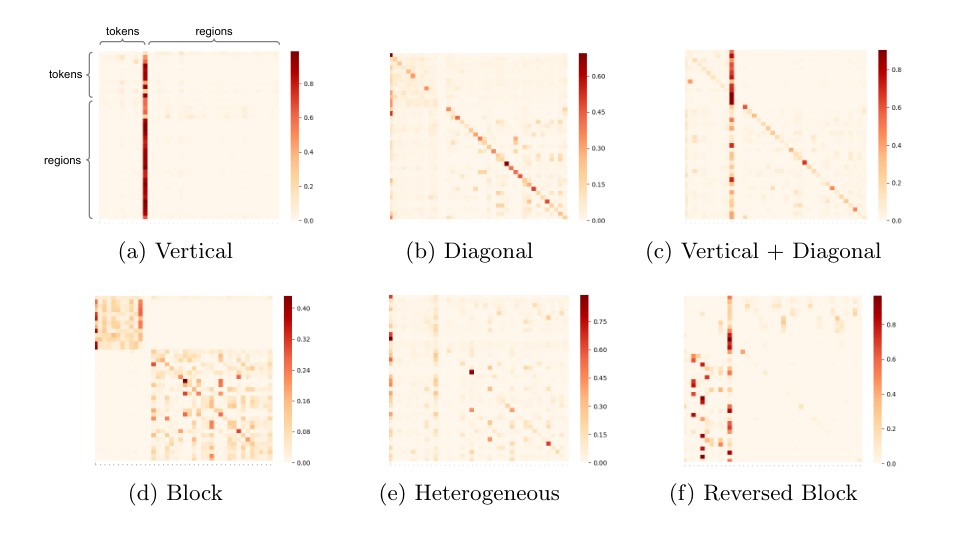
Fig. 2: Visualization of the attention maps learned by the UNITER-base model
图 2:UNITER-base 模型学到的注意力图可视化
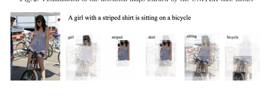
Figure 3: Text-to-image attention visualization example
图 3:文本到图像的注意力可视化示例
4.4 Visualization
4.4 可视化
Similar to [20], we observe several patterns in the attention maps of the UNITER model, as shown in Fig. 2. Note that different from [20], our attention mechanism operates in both inter- and intra-modalitiy manners. For completeness, we briefly discuss each pattern here:
与 [20] 类似,我们在 UNITER 模型的注意力图中观察到若干模式,如图 2 所示。需要注意的是,与 [20] 不同,我们的注意力机制同时在模态间和模态内起作用。为完整起见,这里简要讨论每一种模式:
- • Vertical: attention to special tokens [CLS] or [SEP];
- • 纵向:对特殊词元 [CLS] 或 [SEP] 的注意力;
- • Diagonal: attention to the token/region itself or preceding/following tokens/regions;
- • 对角:对词元/区域自身,或对前一个/后一个词元/区域的注意力;
- • Vertical + Diagonal: mixture of vertical and diagonal;
- • 纵向 + 对角:纵向与对角的混合;
- • Block: intra-modality attention, i.e., textual self-attention and visual self-attention;
- • 分块:模态内注意力,也就是文本自注意力和视觉自注意力;
- • Heterogeneous: diverse attentions that cannot be categorized and is highly dependent on actual input;
- • 异构:无法归类、并高度依赖实际输入的多样注意力;
- • Reversed Block: inter-modality attention, i.e., text-to-image and image-to-text attention.
- • 反向分块:模态间注意力,也就是文本到图像以及图像到文本的注意力。
Note that Reversed Block (Fig. 2(f)) shows cross-modality alignment between tokens and regions. In Fig. 3, we visualize several examples of text-to-image attention to demonstrate the local cross-modality alignment between regions and tokens.
需要注意的是,反向分块(图 2(f))展现了词元与区域之间的跨模态对齐。在图 3 中,我们可视化了若干文本到图像注意力的例子,以说明区域与词元之间的局部跨模态对齐。
5 Conclusion
5 结论
In this paper, we present UNITER, a large-scale pre-trained model providing UNiversal Image-TExt Representations for Vision-and-Language tasks. Four main pre-training tasks are proposed and evaluated through extensive ablation studies. Trained with both in-domain and out-of-domain datasets, UNITER outperforms state-of-the-art models over multiple V+L tasks by a significant margin. Future work includes studying early interaction between raw image pixels and sentence tokens, as well as developing more effective pre-training tasks.
本文提出 UNITER,这是一个大规模预训练模型,为视觉-语言任务提供通用的图像-文本表征。我们提出了四项主要的预训练任务,并通过大量消融对它们做了评估。在域内和域外数据集上训练后,UNITER 在多项 V+L 任务上以显著幅度超过当时最好的模型。未来工作包括研究原始图像像素与句子词元之间的早期交互,以及设计更有效的预训练任务。
References
参考文献
[1] Alberti, C., Ling, J., Collins, M., Reitter, D.: Fusion of detected objects in text for visual question answering. In: EMNLP (2019)
[2] Anderson, P., He, X., Buehler, C., Teney, D., Johnson, M., Gould, S., Zhang, L.: Bottom-up and top-down attention for image captioning and visual question answering. In: CVPR (2018)
[3] Antol, S., Agrawal, A., Lu, J., Mitchell, M., Batra, D., Zitnick, C.L., Parikh, D.: VQA: Visual Question Answering. In: ICCV (2015)
[4] Arjovsky, M., Chintala, S., Bottou, L.: Wasserstein generative adversarial networks. In: ICML (2017)
[5] Boyd, S., Vandenberghe, L.: Convex optimization. Cambridge university press (2004)
[6] Cao, J., Gan, Z., Cheng, Y., Yu, L., Chen, Y.C., Liu, J.: Behind the scene: Revealing the secrets of pre-trained vision-and-language models. arXiv preprint arXiv:2005.07310 (2020)
[7] Chen, L., Gan, Z., Cheng, Y., Li, L., Carin, L., Liu, J.: Graph optimal transport for cross-domain alignment. In: ICML (2020)
[8] Cuturi, M.: Sinkhorn distances: Lightspeed computation of optimal transport. In: NIPS (2013)
[9] Devlin, J., Chang, M.W., Lee, K., Toutanova, K.: Bert: Pre-training of deep bidirectional transformers for language understanding. In: NAACL (2019)
[10] Doersch, C., Gupta, A., Efros, A.A.: Unsupervised visual representation learning by context prediction. In: ICCV (2015)
[11] Fukui, A., Park, D.H., Yang, D., Rohrbach, A., Darrell, T., Rohrbach, M.: Multimodal compact bilinear pooling for visual question answering and visual grounding. In: EMNLP (2017)
[12] Gan, Z., Chen, Y.C., Li, L., Zhu, C., Cheng, Y., Liu, J.: Large-scale adversarial training for vision-and-language representation learning. arXiv preprint arXiv:2006.06195 (2020)
[13] Gao, P., Jiang, Z., You, H., Lu, P., Hoi, S.C., Wang, X., Li, H.: Dynamic fusion with intra-and inter-modality attention flow for visual question answering. In: CVPR (2019)
[14] Genevay, A., Peyré, G., Cuturi, M.: Learning generative models with sinkhorn divergences. In: AISTATS (2018)
[15] Gidaris, S., Singh, P., Komodakis, N.: Unsupervised representation learning by predicting image rotations. In: ICLR (2018)
[16] Hinton, G., Vinyals, O., Dean, J.: Distilling the knowledge in a neural network. arXiv preprint arXiv:1503.02531 (2015)
[17] Karpathy, A., Fei-Fei, L.: Deep visual-semantic alignments for generating image descriptions. In: CVPR (2015)
[18] Kazemzadeh, S., Ordonez, V., Matten, M., Berg, T.: Referitgame: Referring to objects in photographs of natural scenes. In: EMNLP (2014)
[19] Kim, J.H., Jun, J., Zhang, B.T.: Bilinear attention networks. In: NeurIPS (2018)
[20] Kovaleva, O., Romanov, A., Rogers, A., Rumshisky, A.: Revealing the dark secrets of bert. In: EMNLP (2019)
[21] Krishna, R., Zhu, Y., Groth, O., Johnson, J., Hata, K., Kravitz, J., Chen, S., Kalantidis, Y., Li, L.J., Shamma, D.A., et al.: Visual genome: Connecting language and vision using crowdsourced dense image annotations. IJCV (2017)
[22] Lan, Z., Chen, M., Goodman, S., Gimpel, K., Sharma, P., Soricut, R.: Albert: A lite bert for self-supervised learning of language representations. In: ICLR (2020)
[23] Lee, K.H., Chen, X., Hua, G., Hu, H., He, X.: Stacked cross attention for image-text matching. In: ECCV (2018)
[24] Li, G., Duan, N., Fang, Y., Jiang, D., Zhou, M.: Unicoder-vl: A universal encoder for vision and language by cross-modal pre-training. In: AAAI (2020)
[25] Li, L.H., Yatskar, M., Yin, D., Hsieh, C.J., Chang, K.W.: Visualbert: A simple and performant baseline for vision and language. arXiv preprint arXiv:1908.03557 (2019)
[26] Lin, T.Y., Maire, M., Belongie, S., Hays, J., Perona, P., Ramanan, D., Dollár, P., Zitnick, C.L.: Microsoft coco: Common objects in context. In: ECCV (2014)
[27] Liu, Y., Ott, M., Goyal, N., Du, J., Joshi, M., Chen, D., Levy, O., Lewis, M., Zettlemoyer, L., Stoyanov, V.: Roberta: A robustly optimized bert pretraining approach. arXiv preprint arXiv:1907.11692 (2019)
[28] Loshchilov, I., Hutter, F.: Decoupled weight decay regularization. In: ICLR (2019)
[29] Lu, J., Batra, D., Parikh, D., Lee, S.: Vilbert: Pretraining task-agnostic visiolinguistic representations for vision-and-language tasks. In: NeurIPS (2019)
[30] Lu, J., Goswami, V., Rohrbach, M., Parikh, D., Lee, S.: 12-in-1: Multi-task vision and language representation learning. In: CVPR (2020)
[31] Noroozi, M., Favaro, P.: Unsupervised learning of visual representations by solving jigsaw puzzles. In: ECCV (2016)
[32] Ordonez, V., Kulkarni, G., Berg, T.L.: Im2text: Describing images using 1 million captioned photographs. In: NeurIPS (2011)
[33] Ott, M., Edunov, S., Grangier, D., Auli, M.: Scaling neural machine translation. WMT (2018)
[34] Paszke, A., Gross, S., Chintala, S., Chanan, G., Yang, E., DeVito, Z., Lin, Z., Desmaison, A., Antiga, L., Lerer, A.: Automatic differentiation in pytorch (2017)
[35] Pathak, D., Krahenbuhl, P., Donahue, J., Darrell, T., Efros, A.A.: Context encoders: Feature learning by inpainting. In: CVPR (2016)
[36] Peters, M.E., Neumann, M., Iyyer, M., Gardner, M., Clark, C., Lee, K., Zettlemoyer, L.: Deep contextualized word representations. In: NAACL (2018)
[37] Peyré, G., Cuturi, M., et al.: Computational optimal transport. Foundations and Trends® in Machine Learning 11 (5-6), 355–607 (2019)
[38] Plummer, B.A., Wang, L., Cervantes, C.M., Caicedo, J.C., Hockenmaier, J., Lazebnik, S.: Flickr30k entities: Collecting region-to-phrase correspondences for richer image-to-sentence models. In: ICCV (2015)
[39] Radford, A., Wu, J., Child, R., Luan, D., Amodei, D., Sutskever, I.: Language models are unsupervised multitask learners (2019)
[40] Salimans, T., Zhang, H., Radford, A., Metaxas, D.: Improving GANs using optimal transport. In: ICLR (2018)
[41] Sharma, P., Ding, N., Goodman, S., Soricut, R.: Conceptual captions: A cleaned, hypernymed, image alt-text dataset for automatic image captioning. In: ACL (2018)
[42] Su, W., Zhu, X., Cao, Y., Li, B., Lu, L., Wei, F., Dai, J.: Vl-bert: Pre-training of generic visual-linguistic representations. In: ICLR (2020)
[43] Suhr, A., Artzi, Y.: Nlvr2 visual bias analysis. arXiv preprint arXiv:1909.10411 (2019)
[44] Suhr, A., Zhou, S., Zhang, I., Bai, H., Artzi, Y.: A corpus for reasoning about natural language grounded in photographs. In: ACL (2019)
[45] Sun, C., Baradel, F., Murphy, K., Schmid, C.: Contrastive bidirectional transformer for temporal representation learning. arXiv preprint arXiv:1906.05743 (2019)
[46] Sun, C., Myers, A., Vondrick, C., Murphy, K., Schmid, C.: Videobert: A joint model for video and language representation learning. In: ICCV (2019)
[47] Tan, H., Bansal, M.: Lxmert: Learning cross-modality encoder representations from transformers. In: EMNLP (2019)
[48] Trinh, T.H., Luong, M.T., Le, Q.V.: Selfie: Self-supervised pretraining for image embedding. arXiv preprint arXiv:1906.02940 (2019)
[49] Vaswani, A., Shazeer, N., Parmar, N., Uszkoreit, J., Jones, L., Gomez, A.N., Kaiser, Ł., Polosukhin, I.: Attention is all you need. In: NeurIPS (2017)
[50] Wang, L., Li, Y., Lazebnik, S.: Learning deep structure-preserving image-text embeddings. In: CVPR (2016)
[51] Wu, Y., Schuster, M., Chen, Z., Le, Q.V., Norouzi, M., Macherey, W., Krikun, M., Cao, Y., Gao, Q., Macherey, K., et al.: Google’s neural machine translation system: Bridging the gap between human and machine translation. arXiv preprint arXiv:1609.08144 (2016)
[52] Xie, N., Lai, F., Doran, D., Kadav, A.: Visual entailment: A novel task for fine-grained image understanding. arXiv preprint arXiv:1901.06706 (2019)
[53] Xie, Y., Wang, X., Wang, R., Zha, H.: A fast proximal point method for Wasserstein distance. In: arXiv:1802.04307 (2018)
[54] Yang, Z., Dai, Z., Yang, Y., Carbonell, J., Salakhutdinov, R., Le, Q.V.: Xlnet: Generalized autoregressive pretraining for language understanding. In: NeurIPS (2019)
[55] Yu, L., Lin, Z., Shen, X., Yang, J., Lu, X., Bansal, M., Berg, T.L.: Mattnet: Modular attention network for referring expression comprehension. In: CVPR (2018)
[56] Yu, L., Poirson, P., Yang, S., Berg, A.C., Berg, T.L.: Modeling context in referring expressions. In: ECCV (2016)
[57] Yu, Z., Yu, J., Cui, Y., Tao, D., Tian, Q.: Deep modular co-attention networks for visual question answering. In: CVPR (2019)
[58] Zellers, R., Bisk, Y., Farhadi, A., Choi, Y.: From recognition to cognition: Visual commonsense reasoning. In: CVPR (2019)
[59] Zhang, R., Isola, P., Efros, A.A.: Colorful image colorization. In: ECCV (2016)
[60] Zhou, L., Palangi, H., Zhang, L., Hu, H., Corso, J.J., Gao, J.: Unified vision-language pre-training for image captioning and vqa. In: AAAI (2020)
Appendix 0.A Appendix
附录 0.A 附录
This supplementary material has eight sections. Section 0.A.1 describes the details of our dataset collection. Section 0.A.2 describes our implementation details for each downstream task. Section 0.A.3 provides detailed quantitative comparison between conditional masking and joint random masking. Section 0.A.5 provides more results on VCR and NLVR2. Section 0.A.6 provides a direct comparison to VLBERT and ViLBERT. Section 0.A.7 provides some background on optimal transport (OT) and the IPOT algorithm that is used to calculate the OT distance. Section 0.A.8 provides additional visualization example.
这份补充材料共有八节。第 0.A.1 节说明我们收集数据集的细节。第 0.A.2 节说明各下游任务的实现细节。第 0.A.3 节提供条件掩码与联合随机掩码之间更细致的定量比较。第 0.A.5 节提供 VCR 和 NLVR2 上的更多结果。第 0.A.6 节提供与 VLBERT 和 ViLBERT 的直接比较。第 0.A.7 节介绍最优传输(OT)以及用于计算 OT 距离的 IPOT 算法的一些背景。第 0.A.8 节提供补充的可视化例子。
0.A.1 Dataset Collection
0.A.1 数据集收集
As introduced, our full dataset is composed of four existing V+L datasets: COCO, Visual Genome, Conceptual Captions, and SBU Captions. The dataset collection is not simply combining them, as we need to make sure none of the downstream evaluation images are seen during pre-training. Among them, COCO is the most tricky one to clean, as several downstream tasks are built based on it. Figure 4 lists the splits from VQA, Image-Text Retrieval, COCO Captioning, RefCOCO/RefCOCO+/RefCOCOg, and the bottom-up top-down (BUTD) detection [2], all from COCO images.
如前所述,我们的完整数据集由已有的四份 V+L 数据组成:COCO、Visual Genome、Conceptual Captions 和 SBU Captions。收集过程并不是简单把它们合在一起,因为我们需要确保下游评估中的任何图像都不会在预训练中出现。其中,COCO 最需要仔细清理,因为有好几项下游任务都建立在它上面。图 4 列出了 VQA、图文检索、COCO 图像描述、RefCOCO/RefCOCO+/RefCOCOg,以及自下而上自上而下(BUTD)检测 [2] 的各个划分,它们都来自 COCO 图像。
As observed, the validation and test splits of different tasks are scattered across the raw COCO splits. Therefore, we exclude all those evaluation images that appeared in the downstream tasks. In addition, we also exclude all co-occurring Flickr30K images via URL matching, making sure the zero-shot image-text retrieval evaluation on Flickr is fair. The remaining images become the COCO subset within our full dataset, as shown in Figure 4 bottom row. We apply the same rules to Visual Genome, Conceptual Captions, and SBU Captions.
可以看到,不同任务的验证和测试划分散布在原始的 COCO 划分之中。因此,我们排除了所有出现在下游任务中的评估图像。此外,我们还通过 URL 匹配排除了所有同时出现的 Flickr30K 图像,以确保 Flickr 上的零样本图文检索评估是公平的。剩下的图像成为我们完整数据集中的 COCO 子集,如图 4 最下行所示。我们对 Visual Genome、Conceptual Captions 和 SBU Captions 应用了同样的规则。
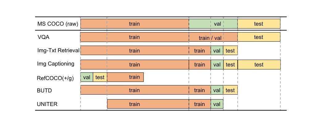
Figure 4: Different data splits from downstream tasks based on COCO images. Our UNITER pre-training avoids seeing any downstream evaluation images
图 4:基于 COCO 图像的下游任务中的不同数据划分。我们的 UNITER 预训练避免看到任何下游评估图像
| Task | Datasets | Image Src. | #Images | #Text | Metric | |
|---|---|---|---|---|---|---|
| 1 | VQA | VQA | COCO | 204K | 1.1M | VQA-score |
| 2 | VCR | VCR | Movie Clips | 110K | 290K | Accuracy |
| 3 | NLVR2 | NLVR2 | Web Crawled | 214K | 107K | Accuracy |
| 4 | Visual Entailment | SNLI-VE | Flickr30K | 31K | 507K | Accuracy |
| 5 | Image-Text Retrieval | COCO | COCO | 92K | 460K | Recall@1,5,10 |
| Flickr30K | Flickr30K | 32K | 160K | |||
| 6 | RE Comprehension | RefCOCO | COCO | 20K | 142K | Accuracy |
| RefCOCO+ | 20K | 142K | ||||
| RefCOCOg | 26K | 95K |
Table 6: Statistics on the datasets of downstream tasks
| 任务 | 数据集 | 图像来源 | 图像数 | 文本数 | 指标 | |
|---|---|---|---|---|---|---|
| 1 | VQA | VQA | COCO | 204K | 1.1M | VQA-score |
| 2 | VCR | VCR | 电影片段 | 110K | 290K | 准确率 |
| 3 | NLVR2 | NLVR2 | 网络抓取 | 214K | 107K | 准确率 |
| 4 | 视觉蕴含 | SNLI-VE | Flickr30K | 31K | 507K | 准确率 |
| 5 | 图文检索 | COCO | COCO | 92K | 460K | Recall@1,5,10 |
| Flickr30K | Flickr30K | 32K | 160K | |||
| 6 | 指称理解 | RefCOCO | COCO | 20K | 142K | 准确率 |
| RefCOCO+ | 20K | 142K | ||||
| RefCOCOg | 26K | 95K |
表 6:下游任务数据集的统计
0.A.2 Implementation Details
0.A.2 实现细节
Our models are implemented based on PyTorch[^17] [34]. To speed up training, we use Nvidia Apex[^18] for mixed precision training. All pre-training experiments are run on Nvidia V100 GPUs (16GB VRAM; PCIe connection). Finetuning experiments are implemented on the same hardware or Titan RTX GPUs (24GB VRAM). To further speed up training, we implement dynamic sequence length to reduce padding and batch examples by number of input units (text tokens + image regions). For large pre-training experiments, we use Horovod[^19] + NCCL[^20] for multi-node communications (on TCP connections through ethernet) with up to 4 nodes of 4x V100 server. Gradient accumulation [33] is also applied to reduce multi-GPU communication overheads.
我们的模型基于 PyTorch[^17] [34] 实现。为加快训练,我们使用 Nvidia Apex[^18] 做混合精度训练。全部预训练实验都在 Nvidia V100 GPU(16GB 显存;PCIe 连接)上运行。微调实验在相同硬件或 Titan RTX GPU(24GB 显存)上完成。为进一步加快训练,我们实现了动态序列长度以减少填充,并按输入单元数(文本词元 + 图像区域)来组批。对大规模预训练实验,我们使用 Horovod[^19] + NCCL[^20] 做多机通信(经以太网的 TCP 连接),最多使用 4 台、每台 4 块 V100 的服务器。同时也使用梯度累积 [33],以降低多 GPU 通信开销。
Visual Question Answering (VQA) We follow [57] to take most frequent answers as answer candidates, and assign a soft target score to each candidate based on its relevancy to the human responses. To finetune on VQA dataset, we use a binary cross-entropy loss to train a multi-label classifier using batch size of input units over maximum K steps. We use AdamW optimizer [28] with a learning rate of and weight decay of . At inference time, the max-probable answer is selected as the predicted answer. For results on test-dev and test-std splits, both training and validation sets are used for training, and additional question-answer pairs from Visual Genome are used for data augmentation as in [57].
视觉问答(VQA) 我们沿用 [57],把出现频率最高的 个答案作为候选,并根据每个候选与 个人工回复的相关程度,给它赋一个软目标分数。在 VQA 数据集上微调时,我们用二元交叉熵损失训练一个多标签分类器,批量大小为 个输入单元,最多训练 K 步。我们使用 AdamW 优化器 [28],学习率为 ,权重衰减为 。推理时,选取概率最大的答案作为预测。对 test-dev 和 test-std 划分上的结果,训练时同时使用训练集和验证集,并像 [57] 那样,额外用 Visual Genome 中的问答对做数据增强。
Visual Commonsense Reasoning (VCR) VCR can be decomposed into two multiple-choice sub-tasks: question-answering task (Q A) and answer-justification task (QA R). In the holistic setting (Q AR), a model needs to first choose an answer from the answer choices, then select a supporting rationale from rationale choices if the chosen answer is correct. We train our model in two settings simultaneously. When testing in the holistic setting, we first apply the model to predict an answer, then obtain the rationale from the same model based on the given question and the predicted answer. To finetune on VCR dataset, we concatenate the question (the qeustion and the ground truth answer) and each answer (rationale) choice from the four possible answer (rationale) candidates. The ‘modality embedding’ is extended to help distinguish question, answer and rationale. Cross-entropy loss is used to train a classifier over two classes (‘‘right’’ or ‘‘wrong’’) for each question-answer pair (question-answer-rationale triplet) with a batch size of 4096 input units over maximum K steps. We use AdamW optimizer with a learning rate of and weight decay of .
视觉常识推理(VCR) VCR 可以分解成两个多选子任务:问答任务(Q A)和答案论证任务(QA R)。在整体设定(Q AR)中,模型需要先从答案选项中选出一个答案,若所选答案正确,再从理由选项中选出一条支持性理由。我们同时在两种设定下训练模型。在整体设定下测试时,我们先用模型预测答案,再根据给定问题和预测出的答案,用同一个模型得到理由。在 VCR 数据集上微调时,我们把问题(该问题以及真实答案)与四个可能的答案(理由)候选中的每一个答案(理由)选项拼接起来。我们对“模态嵌入”做了扩展,以帮助区分问题、答案和理由。对每个问答对(问题-答案-理由三元组),用交叉熵损失训练一个两类(“对”或“错”)分类器,批量大小为 4096 个输入单元,最多训练 K 步。我们使用 AdamW 优化器,学习率为 ,权重衰减为 。
Since the images and text in VCR dataset are very different from our pre-training dataset, we further pre-train our model on VCR, using MLM, MRFR and MRC-kl as the pre-training tasks. ITM is discarded because the text in VCR does not explicitly describe the image. The results of both pre-trainings on VCR are reported in Table 5 (in the main paper) and discussed in the main text. In conclusion, for downstream tasks that contain new data which is very different from the pre-training datasets, second-stage pre-training helps further boost the performance.
由于 VCR 数据集中的图像和文本与我们的预训练数据很不相同,我们进一步在 VCR 上对模型做预训练,使用的预训练任务是 MLM、MRFR 和 MRC-kl。ITM 被去掉,因为 VCR 中的文本并不显式描述图像。两次在 VCR 上预训练的结果报告于表 5(见正文),并在正文中讨论。结论是:对于包含与预训练数据集很不相同的新数据的下游任务,第二阶段预训练有助于进一步提升性能。
In our implementation, the second-stage pre-training is implemented with a batch size of 4096 intput units, a learning rate of and a weight decay of over maximum K steps. After second-stage pre-traing, we finetune our model with a learning rate of over maximum K steps.
在我们的实现中,第二阶段预训练的批量大小为 4096 个输入单元,学习率为 ,权重衰减为 ,最多训练 K 步。第二阶段预训练之后,我们以 的学习率微调模型,最多训练 K 步。
Natural Language for Visual Reasoning for Real (NLVR2) NLVR is a new challenging task for visual reasoning. The goal is to determine whether a natural language statement is true about the given image pair. Here we discuss the three architecture variants of NLVR2 finetuning in detail. Since UNITER only handles one image and one text input at pre-training, the ‘modality embedding’ is extended to help distinguish the additional image presented in the NLVR2 task. For the Triplet setup, we concatenate the image regions and then feed into the UNITER model. An MLP transform is applied on the [CLS] output for binary classification. For the Pair setup, we treat one input example as two text-image pairs by repeating the text. The two [CLS] outputs from UNITER are then depth concatenated as the joint embedding for the example. Another MLP further transform this embedding for the final classification. For the Pair-biattn setup, the input format is the same as the Pair setup. As for the joint representation, instead of rely on only two [CLS] outputs, we apply a multi-head attention layer [49] on one sequence of joint image-text embeddings to attend to the other sequence of embeddings, and vice versa. After this ‘bidirectional’ attention interactions, a simple attentional pooling is applied on each output sequences and then a final concat+MLP layer transforms the cross-attended joint representation for true/false classification.
面向真实图像的自然语言视觉推理(NLVR2) NLVR 是一项新的、有挑战性的视觉推理任务。目标是判断一条自然语言陈述对于给定的图像对是否为真。这里我们详细讨论 NLVR2 微调的三种结构变体。由于 UNITER 在预训练时只处理一张图像和一段文本输入,我们对“模态嵌入”做了扩展,以帮助区分 NLVR2 任务中多出来的那张图像。在 Triplet 设定下,我们把图像区域拼接后送入 UNITER 模型,再对 [CLS] 输出做 MLP 变换,用于二分类。在 Pair 设定下,我们通过重复文本,把一个输入样例当成两个文本-图像对。UNITER 得到的两个 [CLS] 输出再沿深度方向拼接,作为该样例的联合嵌入。另一个 MLP 再变换这一嵌入,用于最终分类。在 Pair-biattn 设定下,输入格式与 Pair 设定相同。至于联合表征,我们不再只依赖两个 [CLS] 输出,而是用一层多头注意力 [49],让一个联合图文嵌入序列去注意另一个嵌入序列,再反过来做一次。经过这种“双向”的注意力交互后,对每个输出序列做简单的注意力汇聚,最后再用一层拼接+MLP,把经过交叉注意的联合表征变换为真/假分类。
We finetune UNITER on NLVR2 for 8K steps with a batch size of 10K input units. AdamW optimizer is used with learning rate of and weight decay of .
我们在 NLVR2 上微调 UNITER 共 8K 步,批量大小为 10K 个输入单元。使用 AdamW 优化器,学习率为 ,权重衰减为 。
Image-Text Retrieval Two datasets are considered for this task: COCO and Flickr30K. COCO consists of K images, each accompanied with five human-written captions. We follow [17] to split the data into 82K/5K/5K training/ validation/test images. Additional 30K images from MSCOCO validation set are also included to improve training as in [23]. Flickr30K dataset contains 31K images collected from the Flickr website, with five textual descriptions per image. We follow [17] to split the data into 30K/1K/1K training/validation/test splits. During finetuning, we sample two negative image-text pairs per positive sample from image and text sides, respectively. For COCO, we use batch size of 60 examples, learning rate of and finetune our model for K steps. For Flickr30K, we finetune our model with a batch size of 120 examples and a learning rate of over maximum K steps.
图文检索 这项任务考虑两份数据集:COCO 和 Flickr30K。COCO 包含 K 张图像,每张配有五条人工撰写的描述。我们沿用 [17],把数据划分为 82K/5K/5K 的训练/验证/测试图像。还像 [23] 那样,额外纳入 MSCOCO 验证集中的 30K 张图像以加强训练。Flickr30K 包含从 Flickr 网站收集的 31K 张图像,每张有五条文本描述。我们沿用 [17],划分为 30K/1K/1K 的训练/验证/测试划分。微调时,我们分别从图像侧和文本侧,为每个正样本采样两个负图文对。对 COCO,批量大小为 60 个样例,学习率为 ,微调 K 步。对 Flickr30K,批量大小为 120 个样例,学习率为 ,最多微调 K 步。
To obtain the final results in Table 3 in the main text, we further sample hard negatives to facilitate the finetuning. For every steps, we randomly sample 128 negative images per text input and obtain a sparse scoring matrix for the whole training set. For each image, we choose the top 20 ranked negative sentences as hard negative samples. Similarly, we get 20 hard negative images for each sentence according to their scores. The hard negatives are sent to the model as additional negative samples. In the end, we have two randomly sampled negatives and two hard negative samples per positive sample. is set to 4000 for COCO and 2500 for Flickr30K.
为得到正文表 3 中的最终结果,我们进一步采样困难负例来帮助微调。每隔 步,我们为每个文本输入随机采样 128 张负图像,并为整个训练集得到一个稀疏的打分矩阵。对每张图像,我们选取排名最高的 20 条负句子作为困难负样本。类似地,我们根据分数为每个句子得到 20 张困难负图像。这些困难负例作为额外的负样本送入模型。最终,每个正样本对应两个随机采样的负例和两个困难负例。对 COCO, 取 4000;对 Flickr30K, 取 2500。
Visual Entailment (SNLI-VE) Visual Entailment is a task derived from Flickr30K images and Stanford Natural Language Inference (SNLI) dataset, where the goal is to determine the logical relationship between a natural language statement and an image. Similar to BERT for Natural Language Inference (NLI), we treat SNLI-VE as a three-way classification problem and apply an MLP Transform on [CLS] output. The UNITER model is finetuned using cross-entropy loss. The batch size is set to 10K input units and we use AdamW with learning rate of to train for 3K steps.
视觉蕴含(SNLI-VE) 视觉蕴含这一任务由 Flickr30K 图像和斯坦福自然语言推理(SNLI)数据集派生而来,目标是判断一条自然语言陈述与一张图像之间的逻辑关系。与把 BERT 用于自然语言推理(NLI)类似,我们把 SNLI-VE 当作一个三类分类问题,并对 [CLS] 输出做 MLP 变换。UNITER 用交叉熵损失微调。批量大小设为 10K 个输入单元,我们使用学习率为 的 AdamW,训练 3K 步。
Referring Expression Comprehension We use three referring expression datasets: RefCOCO, RefCOCO+, and RefCOCOg for the evaluation, all collected on COCO images. To finetune UNITER on this task, we add a MLP layer on top of the region outputs from Transformer, to compute the alignment score between the query phrase/sentence and each region. Since only one object is paired with the query phrase/sentence, we apply cross-entropy loss on the normalized alignment scores. The finetuning is efficient - we train the model with a batch size of 64 examples and a learning rate of for only 5 epochs, and achieve state-of-the-art performance.
指称理解 我们用三份指称表达式数据集来评估:RefCOCO、RefCOCO+ 和 RefCOCOg,它们都收集在 COCO 图像上。在该任务上微调 UNITER 时,我们在 Transformer 的区域输出之上加一层 MLP,以计算查询短语/句子与每个区域之间的对齐分数。由于查询短语/句子只与一个物体配对,我们在归一化后的对齐分数上使用交叉熵损失。微调很高效——我们以 64 个样例的批量大小、学习率 只训练 5 个周期,就达到了当时最好的成绩。
Note all works including ours use off-the-shelf object detectors trained on COCO (and Visual Genome) to extract the visual features. While this does not affect other downstream tasks, it raises an issue for RE comprehension, as the val/test images of RefCOCO, RefCOCO+, and RefCOCOg are a subset of COCO’s training split. Strictly, our object detector is not allowed to train with these val/test images. However, just for a “fair” comparison with concurrent works, we ignore this issue and use the same features [2] as the others. We also update the results of MAttNet using this ”contaminated” features, whose accuracy is 1.5% higher than the original one. As aforementioned, the interaction between sentence and image could start from tokens and pixels instead of the extracted features. We leave this study and RE comprehension with strictly correct features to future work.
需要说明的是,包括我们在内的所有工作,都使用在 COCO(以及 Visual Genome)上训练的现成目标检测器来提取视觉特征。这对其他下游任务没有影响,但却给指称理解带来一个问题,因为 RefCOCO、RefCOCO+ 和 RefCOCOg 的验证/测试图像是 COCO 训练划分的子集。严格来说,我们的目标检测器不允许用这些验证/测试图像来训练。不过,只是为了与同期工作做一次“公平”比较,我们忽略了这一问题,并与其他方法使用相同的特征 [2]。我们还用这种“受污染”的特征更新了 MAttNet 的结果,其准确率比原来高出 1.5%。如前所述,句子与图像之间的交互可以从词元和像素开始,而不是从已经提取好的特征开始。我们把这一研究,以及在严格正确的特征下做指称理解,留待未来工作。
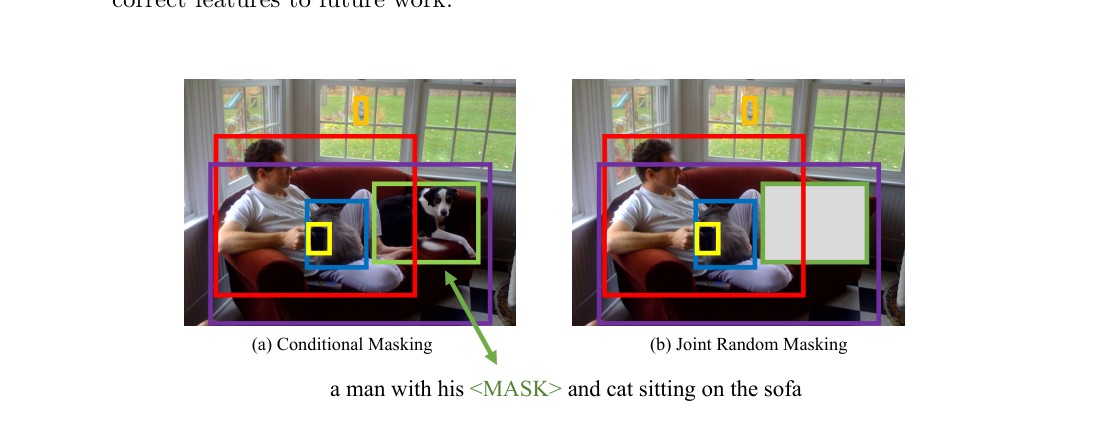
Figure 5: Example showing difference between conditional masking and joint random masking
图 5:展示条件掩码与联合随机掩码差异的例子
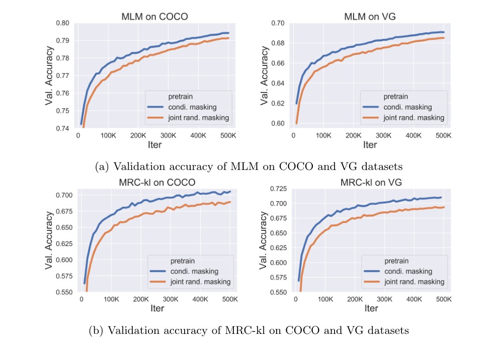
Fig. 6: Comparison of MLM and MRC-kl validation accuracy using joint masking and our proposed conditional masking
图 6:在联合掩码与我们所提出的条件掩码下,MLM 和 MRC-kl 验证准确率的比较
0.A.3 Conditional Masking vs. Joint Random Masking
0.A.3 条件掩码与联合随机掩码
We further discuss the advantage of our proposed conditional masking over joint random masking used in [47, 29]. Intuitively, our conditional masking learns better latent alignment of entities (regions and words) across two modalities. Fig. 5 shows an example image with “man with his dog and cat sitting on a sofa”. With conditional masking, when the region of “dog” is masked, our model should be able to infer that the region is “dog”, based on the context of both surrounding regions and the full sentence (Fig. 5(a)), and vice versa. However, for the joint masking implementation, it could happen when both the region of “dog” and the word “dog” are masked (Fig. 5(b)). In such case, the model has to make the prediction blindly, which might lead to mis-alignment.
我们进一步讨论,相对于 [47, 29] 中使用的联合随机掩码,所提出的条件掩码有何优势。直观上,条件掩码能更好地学习两个模态之间实体(区域和词)的潜在对齐。图 5 给出一个例子,图像内容是“man with his dog and cat sitting on a sofa”。使用条件掩码时,当“dog”这一区域被掩码,我们的模型应当能够根据周围区域以及完整句子的上下文,推断出该区域是“dog”(图 5(a)),反过来也一样。然而,在联合掩码的实现里,有可能“dog”这一区域和“dog”这个词同时被掩码(图 5(b))。在这种情况下,模型只能盲目预测,从而可能导致错位。
To verify this intuition, we show the validation curves during pre-training of MLM and MRC-kl in Fig. 6. Each sub-figure shows a comparison between applying conditional masking and joint random masking during the pre-training of UNITER. The MLM accuracy measures how well UNITER can reconstruct the masked words, and MRC-kl accuracy[^21] measures how well UNITER can classify the masked regions. In both cases, as shown in Fig. 6, our conditional masking converges faster and achieves higher final accuracy than joint random masking. In addition, Table 2 (row 10 & 11) in the main paper shows our conditional masking also performs better on fine-tuned downstream tasks.
为了验证这一直观想法,我们在图 6 中给出预训练期间 MLM 和 MRC-kl 的验证曲线。每个子图都比较了在 UNITER 预训练中使用条件掩码与使用联合随机掩码的差异。MLM 准确率衡量 UNITER 还原被掩码词的能力,MRC-kl 准确率[^21] 衡量 UNITER 分类被掩码区域的能力。在两种情形下,如图 6 所示,我们的条件掩码都收敛更快,最终准确率也高于联合随机掩码。此外,正文表 2(第 10、11 行)表明,我们的条件掩码在微调后的下游任务上也表现更好。
0.A.4 More Ablation Studies on Pre-training Settings
0.A.4 关于预训练设定的更多消融
MRC-only Pre-training
In addition to ablations shown in Table 2 in the main paper, we include results from UNITER-base when pre-trained with MRC only on in-domain data. Table 7 shows that MRC-only pre-training leads to a similar downstream performance to MRFR-only prer-training, which is a weak baseline compared with all other pre-training settings with in-domain data (line 4 - 12 in Table 2).
仅用 MRC 的预训练
除了正文表 2 中的消融之外,我们还给出 UNITER-base 仅用 MRC、在域内数据上预训练的结果。表 7 显示,仅用 MRC 预训练得到的下游表现,与仅用 MRFR 预训练相近,而相对域内数据上的所有其他预训练设定(表 2 第 4 至 12 行),这是一条较弱的基线。
Significance of WRA
In Table 2 of the main paper, we show that adding WRA significantly improves model performance on VQA and RefCOCO+, while achieves comparable results on Flickr and NLVR2. By design, WRA encourages local alignment between each image region and each word in a sentence. Therefore, WRA mostly benefits downstream tasks relying on region-level recognition and reasoning such as VQA, while Flickr and NLVR2 focus more on global rather than local alignments. We add additional ablation results for WRA of UNITER-large when pre-trained with both In-domain and Out-of-domain data in Table 8. We observe large performance gains in zero-shot setup for image/text retrieval and consistent gains across all other tasks.
WRA 的作用
在正文表 2 中我们看到,加入 WRA 能显著提升模型在 VQA 和 RefCOCO+ 上的表现,同时在 Flickr 和 NLVR2 上取得相当的结果。从设计上看,WRA 鼓励每个图像区域与句子中每个词之间的局部对齐。因此,WRA 主要惠及依赖区域级识别和推理的下游任务,例如 VQA;而 Flickr 和 NLVR2 更关注全局而非局部对齐。我们在表 8 中补充了 UNITER-large 在域内加域外数据上预训练时,关于 WRA 的消融结果。我们观察到,在图像/文本检索的零样本设定下有较大提升,并且在所有其他任务上也有稳定的提升。
| Pre-training Data | Pre-training Tasks | Meta-Sum | VQA test-dev | IR (Flickr) val | TR (Flickr) val | NLVR2 dev | RefCOCO+ vald |
|---|---|---|---|---|---|---|---|
| In-domain (COCO+VG) | MRC | 350.97 | 66.23 | 77.17 | 84.57 | 52.31 | 70.69 |
Table 7: Additional ablation results of MRC-only pre-training for UNITER-base with in-domain data.
| 预训练数据 | 预训练任务 | Meta-Sum | VQA test-dev | IR(Flickr)val | TR(Flickr)val | NLVR2 dev | RefCOCO+ vald |
|---|---|---|---|---|---|---|---|
| 域内(COCO+VG) | MRC | 350.97 | 66.23 | 77.17 | 84.57 | 52.31 | 70.69 |
表 7:UNITER-base 仅用 MRC、在域内数据上预训练的补充消融结果。
| WRA pre-train | VQA test-std | NLVR2 test | SNLI-VE test | ZS IR (Flickr) val | ZS TR (Flickr) val | RefCOCO testBd | RefCOCO+ testB | RefCOCOg test |
|---|---|---|---|---|---|---|---|---|
| N | 73.40 | 79.50 | 78.98 | 65.82 | 77.50 | 74.17 | 78.89 | 87.73 |
| Y | 74.02 | 79.98 | 79.38 | 68.74 | 83.60 | 74.98 | 79.75 | 88.47 |
Table 8: A direct ablation on the WRA pre-training task using UNITER-large, all pre-trained on both In-domain + Out-of-domain data, with MLM + ITM + MRC-kl + MRFR (+ WRA). For simplicity, only R@1 is reported for ZS IR and ZS TR.
| 是否做 WRA 预训练 | VQA test-std | NLVR2 test | SNLI-VE test | ZS IR(Flickr)val | ZS TR(Flickr)val | RefCOCO testBd | RefCOCO+ testB | RefCOCOg test |
|---|---|---|---|---|---|---|---|---|
| 否 | 73.40 | 79.50 | 78.98 | 65.82 | 77.50 | 74.17 | 78.89 | 87.73 |
| 是 | 74.02 | 79.98 | 79.38 | 68.74 | 83.60 | 74.98 | 79.75 | 88.47 |
表 8:用 UNITER-large 对 WRA 预训练任务做的直接消融;所有模型都在域内加域外数据上,以 MLM + ITM + MRC-kl + MRFR(+ WRA)预训练。为简洁起见,ZS IR 和 ZS TR 只报告 R@1。
0.A.5 More Results on VCR and NLVR2
0.A.5 VCR 和 NLVR2 上的更多结果
Following the VCR setup in Table 5 of the main paper, we further construct an ensemble model using 10 UNITER-large. Table 9 shows the comparison between VLBERT, ViLBERT and UNITER on VCR. The accuracy of our ensemble model outperforms ViLBERT [29] ensemble by a large margin of 7.0%. Note even single UNITER-large already outperforms ViLBERT ensemble and VLBERT-large by 3.0%.
沿用正文表 5 中的 VCR 设定,我们进一步用 10 个 UNITER-large 构造了一个集成模型。表 9 给出了 VLBERT、ViLBERT 和 UNITER 在 VCR 上的比较。我们的集成模型在 准确率上,以 7.0% 的较大幅度超过 ViLBERT [29] 的集成。需要注意的是,即便单个 UNITER-large 也已经分别超过 ViLBERT 集成和 VLBERT-large 达 3.0%。
Besides, we also compare our UNITER-large with LXMERT [47] and VisualBERT [25] on an additional testing split of NLVR2 in Table 10. Our results consistently outperform the previous SOTA on all metrics[^22] by a large margin of 4.0%.
此外,我们还在表 10 中,把 UNITER-large 与 LXMERT [47] 和 VisualBERT [25] 在 NLVR2 的一个额外测试划分上做了比较。我们的结果在全部指标[^22] 上都以约 的较大幅度超过先前的最好成绩。
| Model | QA | QA R | Q AR |
|---|---|---|---|
| VLBERT-large (single) | 75.8 | 78.4 | 59.7 |
| ViLBERT (10 ensemble) | 76.4 | 78.0 | 59.8 |
| UNITER-large (single) | 77.3 | 80.8 | 62.8 |
| UNITER-large (10 ensemble) | 79.8 | 83.4 | 66.8 |
Table 9: VCR results from VLBERT [42], ViLBERT [29], and UNITER
| 模型 | QA | QAR | QAR |
|---|---|---|---|
| VLBERT-large(单模型) | 75.8 | 78.4 | 59.7 |
| ViLBERT(10 模型集成) | 76.4 | 78.0 | 59.8 |
| UNITER-large(单模型) | 77.3 | 80.8 | 62.8 |
| UNITER-large(10 模型集成) | 79.8 | 83.4 | 66.8 |
表 9:VLBERT [42]、ViLBERT [29] 和 UNITER 在 VCR 上的结果
| Model | Balanced | Unbalanced | Overall | Consistency |
|---|---|---|---|---|
| VisualBERT | 67.3 | 68.2 | 67.3 | 26.9 |
| LXMERT | 76.6 | 76.5 | 76.2 | 42.1 |
| UNITER-large | 80.0 | 81.2 | 80.4 | 50.8 |
Table 10: NLVR2 results on test-U split from VisualBERT [25], LXMERT [47], and UNITER
| 模型 | Balanced | Unbalanced | Overall | Consistency |
|---|---|---|---|---|
| VisualBERT | 67.3 | 68.2 | 67.3 | 26.9 |
| LXMERT | 76.6 | 76.5 | 76.2 | 42.1 |
| UNITER-large | 80.0 | 81.2 | 80.4 | 50.8 |
表 10:VisualBERT [25]、LXMERT [47] 和 UNITER 在 NLVR2 的 test-U 划分上的结果
| Model | VQA | RefCOCO+ (det) | ||
|---|---|---|---|---|
| test-dev | val | testA | testB | |
| ViLBERT | 70.55 | 72.34 | 78.52 | 62.61 |
| VLBERT-base | 71.16 | 71.60 | 77.72 | 60.99 |
| UNITER-base | 71.22 | 72.49 | 79.36 | 63.65 |
Table 11: A direct comparison between ViLBERT [29], VLBERT [42], and our UNITER, all trained on Conceptual Captions [41] only
| 模型 | VQA test-dev | RefCOCO+(det)val | RefCOCO+(det)testA | RefCOCO+(det)testB |
|---|---|---|---|---|
| ViLBERT | 70.55 | 72.34 | 78.52 | 62.61 |
| VLBERT-base | 71.16 | 71.60 | 77.72 | 60.99 |
| UNITER-base | 71.22 | 72.49 | 79.36 | 63.65 |
表 11:ViLBERT [29]、VLBERT [42] 与我们的 UNITER 的直接比较,三者都只在 Conceptual Captions [41] 上训练
0.A.6 Direct Comparison to VLBERT and ViLBERT
0.A.6 与 VLBERT 和 ViLBERT 的直接比较
To further demonstrate our idea, we conduct a direct comparison to ViLBERT [29] and VLBERT [42], trained on Conceptual Captions [41]. We pre-train UNITER on Conceptual Captions only using our proposed conditional masking and the best pre-training tasks. Table 11 shows that UNITER still consistently outperforms the other models by a visible margin on VQA and RefCOCO+.
为了进一步说明我们的想法,我们与在 Conceptual Captions [41] 上训练的 ViLBERT [29] 和 VLBERT [42] 做了直接比较。我们只在 Conceptual Captions 上,使用所提出的条件掩码以及最佳预训练任务来预训练 UNITER。表 11 表明,UNITER 在 VQA 和 RefCOCO+ 上仍然以可见的幅度稳定超过其他模型。
0.A.7 Review of Optimal Transport and the IPOT Algorithm
0.A.7 最优传输与 IPOT 算法回顾
Optimal Transport We first provide a brief review of optimal transport, which defines distances between probability measures on a domain (the sequence space in our setting). The optimal transport distance for two probability measures and is defined as [37]:
最优传输 我们先简要回顾最优传输,它定义了定义域 上(在我们的设定里是序列空间)概率测度之间的距离。两个概率测度 和 的最优传输距离定义为 [37]:
where denotes the set of all joint distributions with marginals and ; is the cost function for moving to , e.g., the Euclidean or cosine distance. Intuitively, the optimal transport distance is the minimum cost that induces in order to transport from to . When is a metric on , induces a proper metric on the space of probability distributions supported on , commonly known as the Wasserstein distance. One of the most popular choices is the Wasserstein distance where the squared Euclidean distance is used as cost.
其中 表示所有以 和 为边缘分布的联合分布 的集合; 是把 搬到 的代价函数,例如欧氏距离或余弦距离。直观上,最优传输距离就是 为了从 搬运到 所引起的最小代价。当 是 上的度量时, 会在支撑于 的概率分布空间上诱导出一个真正的度量,通常称为 Wasserstein 距离。最常用的选择之一是 Wasserstein 距离 ,此时使用平方欧氏距离 作为代价。
1: Input: Feature vectors , and generalized stepsize ,
2: ,
3: ,
4: for do
5: // is Hadamard product
6: for do // in practice
7: ,
8: end for
9:
10: end for
11: Return
Algorithm 1 IPOT algorithm
1: 输入: 特征向量 ,,以及广义步长 ,
2: ,
3: ,
4: for do
5: // 表示 Hadamard 积
6: for do // 实践中
7: ,
8: end for
9:
10: end for
11: 返回
算法 1 IPOT 算法
The IPOT algorithm Unfortunately, the exact minimization over is in general computational intractable [4, 14, 40]. To overcome such intractability, we consider an efficient iterative approach to approximate the OT distance. We propose to use the recently introduced Inexact Proximal point method for Optimal Transport (IPOT) algorithm to compute the OT matrix , thus also the OT distance [53]. Specifically, IPOT iteratively solves the following optimization problem using the proximal point method [5]:
IPOT 算法 遗憾的是,对 的精确最小化在一般情况下计算上难以完成 [4, 14, 40]。为克服这一困难,我们采用一种高效的迭代方法来近似 OT 距离。我们使用最近提出的、面向最优传输的不精确近端点方法(IPOT)来计算 OT 矩阵 ,从而也得到 OT 距离 [53]。具体来说,IPOT 用近端点方法 [5] 迭代求解下列优化问题:
where the proximity metric term penalizes solutions that are too distant from the latest approximation, and is understood as the generalized stepsize. This renders a tractable iterative scheme towards the exact OT solution. In this work, we employ the generalized KL Bregman divergence as the proximity metric. Algorithm 1 describes the implementation details for IPOT.
其中邻近度量项 会惩罚与最近一次近似相距过远的解, 则被理解为广义步长。这就给出了一种通向精确 OT 解、且计算上可行的迭代格式。本文采用广义 KL Bregman 散度 作为邻近度量。算法 1 给出了 IPOT 的实现细节。
Note that the Sinkhorn algorithm [8] can also be used to compute the OT matrix. Specifically, the Sinkhorn algorithm tries to solve the entropy regularized optimization problem: where is the entropy regularization term and is the regularization strength. However, in our experiments, we empirically found that the numerical stability and performance of the Sinkhorn algorithm is quite sensitive to the choice of the hyper-parameter , thus only IPOT is considered in our model training.
需要说明的是,Sinkhorn 算法 [8] 也可以用来计算 OT 矩阵。具体来说,Sinkhorn 算法试图求解带熵正则的优化问题:,其中 是熵正则项, 是正则强度。不过在我们的实验中,我们经验上发现 Sinkhorn 算法的数值稳定性和性能对超参数 的选择相当敏感,因此在模型训练中只考虑 IPOT。
0.A.8 Additional Visualization
0.A.8 补充可视化
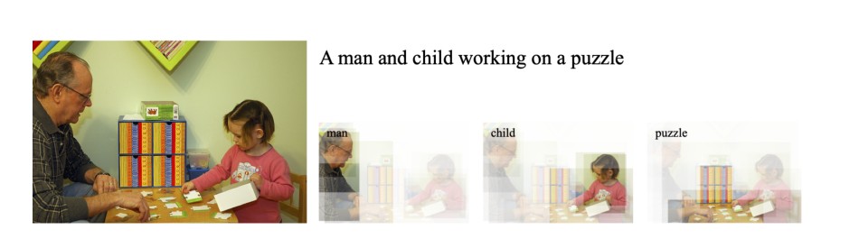
Figure 7: Additional text-to-image attention visualization example
图 7:补充的文本到图像注意力可视化示例
Footnotes
脚注
[^1] Code is available at https://github.com/ChenRocks/UNITER.
[^2] Our Faster R-CNN was pre-trained on Visual Genome object+attribute data [2].
[^3] (normalized top/left/bottom/right coordinates, width, height, and area.)
[^4] We use word/sub-word and token interchangeably throughout the rest of the paper.
[^5] We also use a special modality embedding to help the model distinguish between textual and visual input, which is similar to the ‘segment embedding’ in BERT. This embedding is also summed before the LN layer in each embedder. For simplicity, this modality embedding is omitted in Figure 1.
[^6] is the natural numbers, is the number of masked tokens, and is the set of masked indices.
[^7] Following BERT, we decompose this 15% into 10% random words, 10% unchanged, and 80% [MASK].
[^8] Performing this during pre-training also alleviates the mismatch problem between pre-training and downstream finetuning tasks, since most of the downstream tasks take the representation of the [CLS] token as the joint representation.
[^9] A total of 222 images were eliminated through this process.
[^10] We apply the same URL matching method, excluding 109 images from training.
[^11] VQA, VCR, NLVR2, Visual Entailment, Image-Text Retrieval, and Referring Expression Comprehension. Details about the tasks are listed in the supplementary.
[^12] UNITER-base: L=12, H=768, A=12, Total Parameters=86M. UNITER-large: L=24, H=1024, A=16, Total Parameters=303M (L: number of stacked Transformer blocks; H: hidden activation dimension; A: number of attention heads). and V100 GPU hours were used for pre-training UNITER-base and UNITER-large.
[^13] The evaluation splits of RE comprehension using detected proposals are denoted as vald, testd, etc.
[^14] Details about the metrics are listed in the supplementary.
[^15] MAttNet results are updated using the same features as the others. More details are provided in the supplementary file.
[^16] The word embedding layer contains excessive rare words, thus excluded from the parameter counts.
[^17] https://pytorch.org/
[^18] https://github.com/NVIDIA/apex
[^19] https://github.com/horovod/horovod
[^20] https://github.com/NVIDIA/nccl
[^21] When validating on MRC-kl accuracy, we simply pick the most confident category from the predicted probability and measure its correctness.
[^22] The balanced and unbalanced evaluations were introduced in [43].
[^1] 代码见 https://github.com/ChenRocks/UNITER。
[^2] 我们的 Faster R-CNN 在 Visual Genome 的物体+属性数据上预训练 [2]。
[^3] (归一化后的上/左/下/右坐标,以及宽度、高度和面积。)
[^4] 在本文其余部分,我们把词/子词和词元互换使用。
[^5] 我们还使用一种特殊的模态嵌入,帮助模型区分文本输入和视觉输入,这与 BERT 中的“段嵌入”类似。该嵌入也在每个嵌入器的 LN 层之前被加进去。为简洁起见,图 1 中省略了这一模态嵌入。
[^6] 表示自然数, 是被掩码词元的个数, 是被掩码下标的集合。
[^7] 沿用 BERT,我们把这 15% 再拆成:10% 随机词、10% 保持不变、80% 换成 [MASK]。
[^8] 在预训练中这样做,也有助于缓解预训练与下游微调任务之间的不匹配,因为大多数下游任务都把 [CLS] 词元的表示当作联合表征。
[^9] 这一过程共排除了 222 张图像。
[^10] 我们使用同样的 URL 匹配方法,从训练中排除了 109 张图像。
[^11] VQA、VCR、NLVR2、视觉蕴含、图文检索以及指称理解。任务细节见补充材料。
[^12] UNITER-base:L=12,H=768,A=12,总参数量=8600 万。UNITER-large:L=24,H=1024,A=16,总参数量=3.03 亿(L:堆叠的 Transformer 块数;H:隐藏激活维数;A:注意力头数)。预训练 UNITER-base 和 UNITER-large 分别使用了 和 个 V100 GPU 小时。
[^13] 使用检测提议来评估指称理解的划分记为 vald、testd 等。
[^14] 各指标的细节见补充材料。
[^15] MAttNet 的结果已用与其他方法相同的特征更新。更多细节见补充材料。
[^16] 词嵌入层包含过多的罕见词,因而未计入参数量。
[^17] https://pytorch.org/
[^18] https://github.com/NVIDIA/apex
[^19] https://github.com/horovod/horovod
[^20] https://github.com/NVIDIA/nccl
[^21] 在验证 MRC-kl 准确率时,我们只从预测概率中选取置信度最高的类别,并衡量其是否正确。
[^22] 平衡与非平衡评估由 [43] 引入。