Trust Region Policy Optimization
Trust Region Policy Optimization
信赖域策略优化
John Schulman Sergey Levine Philipp Moritz Michael I. Jordan Pieter Abbeel
Abstract
摘要
We describe an iterative procedure for optimizing policies, with guaranteed monotonic improvement. By making several approximations to the theoretically-justified procedure, we develop a practical algorithm, called Trust Region Policy Optimization (TRPO). This algorithm is similar to natural policy gradient methods and is effective for optimizing large nonlinear policies such as neural networks. Our experiments demonstrate its robust performance on a wide variety of tasks: learning simulated robotic swimming, hopping, and walking gaits; and playing Atari games using images of the screen as input. Despite its approximations that deviate from the theory, TRPO tends to give monotonic improvement, with little tuning of hyperparameters.
我们描述一种有单调改进保证的策略迭代优化流程。对理论保证的流程做若干近似后,得到实用算法——信赖域策略优化(Trust Region Policy Optimization,TRPO)。该算法与自然策略梯度方法相近,能有效优化神经网络一类大型非线性策略。实验表明它在多种任务上表现稳健:学习仿真机器人的游泳、跳跃与行走步态,以及用屏幕图像作输入玩 Atari 游戏。尽管近似偏离了理论,TRPO 仍往往给出单调改进,且超参几乎不用细调。
1 Introduction
1 引言
Most algorithms for policy optimization can be classified into three broad categories: (1) policy iteration methods, which alternate between estimating the value function under the current policy and improving the policy (Bertsekas 2005); (2) policy gradient methods, which use an estimator of the gradient of the expected return (total reward) obtained from sample trajectories (Peters & Schaal 2008a) (and which, as we later discuss, have a close connection to policy iteration); and (3) derivative-free optimization methods, such as the cross-entropy method (CEM) and covariance matrix adaptation (CMA), which treat the return as a black box function to be optimized in terms of the policy parameters (Szita & Lörincz 2006).
策略优化算法大体可分三类:(1)策略迭代:在当前策略下估计价值函数与改进策略之间交替(Bertsekas 2005);(2)策略梯度:用样本轨迹估计期望回报(总奖励)的梯度(Peters & Schaal 2008a)(后文也会谈到它与策略迭代的密切联系);(3)无导数优化,如交叉熵方法(CEM)与协方差矩阵自适应(CMA),把回报当作策略参数上的黑箱函数来优化(Szita & Lörincz 2006)。
General derivative-free stochastic optimization methods such as CEM and CMA are preferred on many problems, because they achieve good results while being simple to understand and implement. For example, while Tetris is a classic benchmark problem for approximate dynamic programming (ADP) methods, stochastic optimization methods are difficult to beat on this task (Gabillon et al. 2013). For continuous control problems, methods like CMA have been successful at learning control policies for challenging tasks like locomotion when provided with hand-engineered policy classes with low-dimensional parameterizations (Wampler & Popović 2009). The inability of ADP and gradient-based methods to consistently beat gradient-free random search is unsatisfying, since gradient-based optimization algorithms enjoy much better sample complexity guarantees than gradient-free methods (Nemirovski 2005). Continuous gradient-based optimization has been very successful at learning function approximators for supervised learning tasks with huge numbers of parameters, and extending their success to reinforcement learning would allow for efficient training of complex and powerful policies.
在许多问题上,人们更偏爱 CEM、CMA 这类通用无导数随机优化:效果好,又简单易懂、好实现。例如,俄罗斯方块是近似动态规划(ADP)的经典基准,但随机优化方法在该任务上很难被打败(Gabillon et al. 2013)。连续控制里,若策略类由人工设计且参数维度低,CMA 等也能成功学会运动控制(Wampler & Popović 2009)。ADP 与基于梯度的方法无法稳定胜过无梯度随机搜索,这一点令人不满:因为有梯度的优化在样本复杂度保证上远好于无梯度方法(Nemirovski 2005)。连续梯度优化已在参数量巨大的监督学习函数逼近器上非常成功;若能把这一成功延到强化学习,就可高效训练复杂而强大的策略。
In this article, we first prove that minimizing a certain surrogate objective function guarantees policy improvement with non-trivial step sizes. Then we make a series of approximations to the theoretically-justified algorithm, yielding a practical algorithm, which we call trust region policy optimization (TRPO). We describe two variants of this algorithm: first, the single-path method, which can be applied in the model-free setting; second, the vine method, which requires the system to be restored to particular states, which is typically only possible in simulation. These algorithms are scalable and can optimize nonlinear policies with tens of thousands of parameters, which have previously posed a major challenge for model-free policy search (Deisenroth et al. 2013). In our experiments, we show that the same TRPO methods can learn complex policies for swimming, hopping, and walking, as well as playing Atari games directly from raw images.
本文先证明:最小化某一代理目标函数,可在非平凡步长下保证策略改进;再对理论算法做一系列近似,得到实用算法——信赖域策略优化(TRPO)。我们描述两种变体:一是可用于无模型设定的 single-path 方法;二是 vine 方法,要求系统能恢复到特定状态,通常只在仿真中可行。这些算法可扩展,能优化带数万参数的非线性策略——此前这对无模型策略搜索是重大挑战(Deisenroth et al. 2013)。实验中,同一套 TRPO 方法可学会游泳、跳跃、行走的复杂策略,也能直接从原始图像学会玩 Atari。
2 Preliminaries
2 预备知识
Consider an infinite-horizon discounted Markov decision process (MDP), defined by the tuple , where is a finite set of states, is a finite set of actions, is the transition probability distribution, is the reward function, is the distribution of the initial state , and is the discount factor.
考虑无限时域折扣马尔可夫决策过程(MDP),由元组 定义,其中 为有限状态集, 为有限动作集, 为转移概率分布, 为奖励函数, 为初始状态 的分布, 为折扣因子。
Let denote a stochastic policy , and let denote its expected discounted reward:
令 表示随机策略 ,令 表示其期望折扣奖励:
We will use the following standard definitions of the state-action value function , the value function , and the advantage function :
我们将使用状态—动作价值函数 、价值函数 与优势函数 的如下标准定义:
The following useful identity expresses the expected return of another policy in terms of the advantage over , accumulated over timesteps (see Kakade & Langford 2002 or Appendix A for proof):
下面的有用恒等式把另一策略 的期望回报写成相对 的优势在各时间步上的累积(证明见 Kakade & Langford 2002 或附录 A):
where the notation indicates that actions are sampled . Let be the (unnormalized) discounted visitation frequencies
其中记号 表示动作按 采样。令 为(未归一化的)折扣访问频率
where and the actions are chosen according to . We can rewrite Equation 1 with a sum over states instead of timesteps:
其中 ,动作按 选取。我们可把式 (1) 改写成对状态求和而非对时间步求和:
This equation implies that any policy update that has a nonnegative expected advantage at every state , i.e., , is guaranteed to increase the policy performance , or leave it constant in the case that the expected advantage is zero everywhere. This implies the classic result that the update performed by exact policy iteration, which uses the deterministic policy , improves the policy if there is at least one state-action pair with a positive advantage value and nonzero state visitation probability, otherwise the algorithm has converged to the optimal policy. However, in the approximate setting, it will typically be unavoidable, due to estimation and approximation error, that there will be some states for which the expected advantage is negative, that is, . The complex dependency of on makes Equation (2) difficult to optimize directly. Instead, we introduce the following local approximation to :
该式意味着:任意在 每一个 状态 上都有非负期望优势的策略更新 ,即 ,都能保证策略性能 上升,或在处处期望优势为零时保持不变。由此得到经典结论:精确策略迭代所用的确定性策略 ,只要存在至少一个优势为正且状态访问概率非零的状态—动作对,就会改进策略;否则算法已收敛到最优策略。但在近似设定中,由于估计与逼近误差,通常不可避免地会有一些状态 使期望优势为负,即 。 对 的复杂依赖使式 (2) 难以直接优化。于是我们引入如下对 的局部近似:
Note that uses the visitation frequency rather than , ignoring changes in state visitation density due to changes in the policy. However, if we have a parameterized policy , where is a differentiable function of the parameter vector , then matches to first order (see Kakade & Langford 2002). That is, for any parameter value ,
注意 使用访问频率 而非 ,忽略了策略改变引起的状态访问密度变化。不过,若有参数化策略 ,且 对参数向量 可微,则 与 一阶吻合(见 Kakade & Langford 2002)。也即,对任意参数值 ,
Equation 4 implies that a sufficiently small step that improves will also improve , but does not give us any guidance on how big of a step to take.
式 (4) 意味着:充分小的、能改进 的一步 也会改进 ,但并未告诉我们步长可以取多大。
To address this issue, Kakade & Langford 2002 proposed a policy updating scheme called conservative policy iteration, for which they could provide explicit lower bounds on the improvement of . To define the conservative policy iteration update, let denote the current policy, and let . The new policy was defined to be the following mixture:
为处理这一问题,Kakade & Langford 2002 提出名为保守策略迭代的更新方案,并能给出 改进的显式下界。定义保守策略迭代更新:令 为当前策略,令 。新策略 定义为如下混合:
Kakade and Langford derived the following lower bound:
Kakade 与 Langford 导出了如下下界:
(We have modified it to make it slightly weaker but simpler.) Note, however, that so far this bound only applies to mixture policies generated by Equation (5). This policy class is unwieldy and restrictive in practice, and it is desirable for a practical policy update scheme to be applicable to all general stochastic policy classes.
(我们稍作改写,使下界略弱但更简洁。)但注意,目前该界只适用于式 (5) 生成的混合策略。这类策略类在实践中笨拙且受限;实用的策略更新方案最好能适用于一般随机策略类。
3 Monotonic Improvement Guarantee for General Stochastic Policies
3 一般随机策略的单调改进保证
Equation 6, which applies to conservative policy iteration, implies that a policy update that improves the right-hand side is guaranteed to improve the true performance . Our principal theoretical result is that the policy improvement bound in Equation 6 can be extended to general stochastic policies, rather than just mixture polices, by replacing with a distance measure between and , and changing the constant appropriately. Since mixture policies are rarely used in practice, this result is crucial for extending the improvement guarantee to practical problems. The particular distance measure we use is the total variation divergence, which is defined by for discrete probability distributions .[^1] Define as
适用于保守策略迭代的式 (6) 意味着:改进右侧的策略更新保证能改进真实性能 。我们的主要理论结果是:把 换成 与 之间的某种距离度量,并相应改写常数 ,即可把式 (6) 的策略改进界从混合策略推广到一般随机策略。由于实践中很少用混合策略,这一结果对把改进保证延到实际问题至关重要。我们采用的距离度量是全变差散度,对离散概率分布 定义为 。定义 为
Theorem 1.
Let . Then the following bound holds:
定理 1。
令 。则下列界成立:
We provide two proofs in the appendix. The first proof extends Kakade and Langford’s result using the fact that the random variables from two distributions with total variation divergence less than can be coupled, so that they are equal with probability . The second proof uses perturbation theory.
附录给出两种证明。第一种利用全变差散度小于 的两分布随机变量可耦合、从而以概率 相等,来扩展 Kakade 与 Langford 的结果;第二种使用摄动理论。
Next, we note the following relationship between the total variation divergence and the KL divergence (Pollard 2000, Ch. 3): . Let . The following bound then follows directly from 1:
接下来注意全变差散度与 KL 散度的关系(Pollard 2000,第 3 章):。令 。则由定理 1 直接得到如下界:
Algorithm 1 describes an approximate policy iteration scheme based on the policy improvement bound in Equation (9). Note that for now, we assume exact evaluation of the advantage values .
算法 1 描述基于式 (9) 策略改进界的近似策略迭代方案。注意此刻我们假定优势值 可精确求值。
Algorithm 1 Policy iteration algorithm guaranteeing non-decreasing expected return
算法 1 保证期望回报 非降的策略迭代算法
It follows from Equation 9 that Algorithm 1 is guaranteed to generate a monotonically improving sequence of policies . To see this, let . Then
由式 (9) 可知,算法 1 保证生成单调改进的策略序列 。为此令 。则
Thus, by maximizing at each iteration, we guarantee that the true objective is non-decreasing. This algorithm is a type of minorization-maximization (MM) algorithm (Hunter & Lange 2004), which is a class of methods that also includes expectation maximization. In the terminology of MM algorithms, is the surrogate function that minorizes with equality at . This algorithm is also reminiscent of proximal gradient methods and mirror descent.
因此,每步最大化 即可保证真实目标 非降。该算法属于一类称为最小化—最大化(MM)的算法(Hunter & Lange 2004),期望最大化也属此类。按 MM 术语, 是在 处与 相等、并 minorizes 的代理函数。该算法也令人想起近端梯度方法与镜像下降。
Trust region policy optimization, which we propose in the following section, is an approximation to Algorithm 1, which uses a constraint on the KL divergence rather than a penalty to robustly allow large updates.
下一节提出的 信赖域策略优化 是对算法 1 的近似:用 KL 散度约束代替惩罚项,从而稳健地允许较大更新。
4 Optimization of Parameterized Policies
4 参数化策略的优化
In the previous section, we considered the policy optimization problem independently of the parameterization of and under the assumption that the policy can be evaluated at all states. We now describe how to derive a practical algorithm from these theoretical foundations, under finite sample counts and arbitrary parameterizations.
上一节在与 的参数化无关、并假定策略可在所有状态求值的前提下讨论策略优化。现在说明如何在有限样本与任意参数化下,从这些理论基础导出实用算法。
Since we consider parameterized policies with parameter vector , we will overload our previous notation to use functions of rather than , e.g. , , and . We will use to denote the previous policy parameters that we want to improve upon.
由于考虑带参数向量 的参数化策略 ,我们将沿用先前记号,改写成 的函数,例如 ,,以及 。用 表示我们希望改进的上一轮策略参数。
The preceding section showed that , with equality at . Thus, by performing the following maximization, we are guaranteed to improve the true objective :
上一节表明 ,且在 处等号成立。因此做如下最大化即可保证改进真实目标 :
In practice, if we used the penalty coefficient recommended by the theory above, the step sizes would be very small. One way to take larger steps in a robust way is to use a constraint on the KL divergence between the new policy and the old policy, i.e., a trust region constraint:
实践中,若采用理论给出的惩罚系数 ,步长会非常小。一种稳健地迈出更大步的方式,是对新旧策略之间的 KL 散度施加约束,即信赖域约束:
This problem imposes a constraint that the KL divergence is bounded at every point in the state space. While it is motivated by the theory, this problem is impractical to solve due to the large number of constraints. Instead, we can use a heuristic approximation which considers the average KL divergence:
该问题要求状态空间每一点上的 KL 散度都有界。虽有理论动机,但约束数量巨大,不切实际。可改用启发式近似,考虑平均 KL 散度:
We therefore propose solving the following optimization problem to generate a policy update:
因此我们提议解如下优化问题以产生策略更新:
Similar policy updates have been proposed in prior work (Bagnell & Schneider 2003; Peters & Schaal 2008b; Peters et al. 2010), and we compare our approach to prior methods in Section 7 and in the experiments in Section 8. Our experiments also show that this type of constrained update has similar empirical performance to the maximum KL divergence constraint in Equation (11).
类似的策略更新在先前工作中已有提出(Bagnell & Schneider 2003;Peters & Schaal 2008b;Peters et al. 2010),我们在第 7 节与第 8 节实验中与先前方法比较。实验也表明,这类带约束的更新与式 (11) 的最大 KL 散度约束经验表现相近。
5 Sample-Based Estimation of the Objective and Constraint
5 目标与约束的基于样本估计
The previous section proposed a constrained optimization problem on the policy parameters (Equation (12)), which optimizes an estimate of the expected total reward subject to a constraint on the change in the policy at each update. This section describes how the objective and constraint functions can be approximated using Monte Carlo simulation.
上一节提出策略参数上的约束优化问题(式 (12)):在每次更新对策略变化施加约束的前提下,优化期望总奖励 的估计。本节说明如何用蒙特卡洛仿真近似目标函数与约束函数。
We seek to solve the following optimization problem, obtained by expanding in Equation (12):
我们要求解如下优化问题,由式 (12) 展开 得到:
We first replace in the objective by the expectation . Next, we replace the advantage values by the -values in Equation (13), which only changes the objective by a constant. Last, we replace the sum over the actions by an importance sampling estimator. Using to denote the sampling distribution, the contribution of a single to the loss function is
首先把目标中的 换成期望 。再把式 (13) 中的优势值 换成 值 ,这只使目标相差一个常数。最后把对动作的求和换成重要性采样估计。用 表示采样分布,则单个 对损失函数的贡献为
Our optimization problem in Equation 13 is exactly equivalent to the following one, written in terms of expectations:
式 13 中的优化问题与下面用期望写成的问题完全等价:
All that remains is to replace the expectations by sample averages and replace the value by an empirical estimate. The following sections describe two different schemes for performing this estimation.
剩下只需把期望换成样本平均,并把 值换成经验估计。以下两小节描述两种不同的估计方案。
The first sampling scheme, which we call single path, is the one that is typically used for policy gradient estimation (Bartlett & Baxter 2011), and is based on sampling individual trajectories. The second scheme, which we call vine, involves constructing a rollout set and then performing multiple actions from each state in the rollout set. This method has mostly been explored in the context of policy iteration methods (Lagoudakis & Parr 2003; Gabillon et al. 2013).
第一种采样方案称为 single path,是策略梯度估计中常用的做法(Bartlett & Baxter 2011),基于采样单条轨迹。第二种称为 vine,先构造 rollout 集合,再从该集合中每个状态执行多个动作。该方法多在策略迭代语境下被探索(Lagoudakis & Parr 2003;Gabillon et al. 2013)。
5.1 Single Path
In this estimation procedure, we collect a sequence of states by sampling and then simulating the policy for some number of timesteps to generate a trajectory . Hence, . is computed at each state-action pair by taking the discounted sum of future rewards along the trajectory.
该估计流程中,我们采样 ,再按策略 仿真若干时间步,生成轨迹 。于是 。每个状态—动作对 上的 由轨迹上未来奖励的折扣和计算。
5.2 Vine
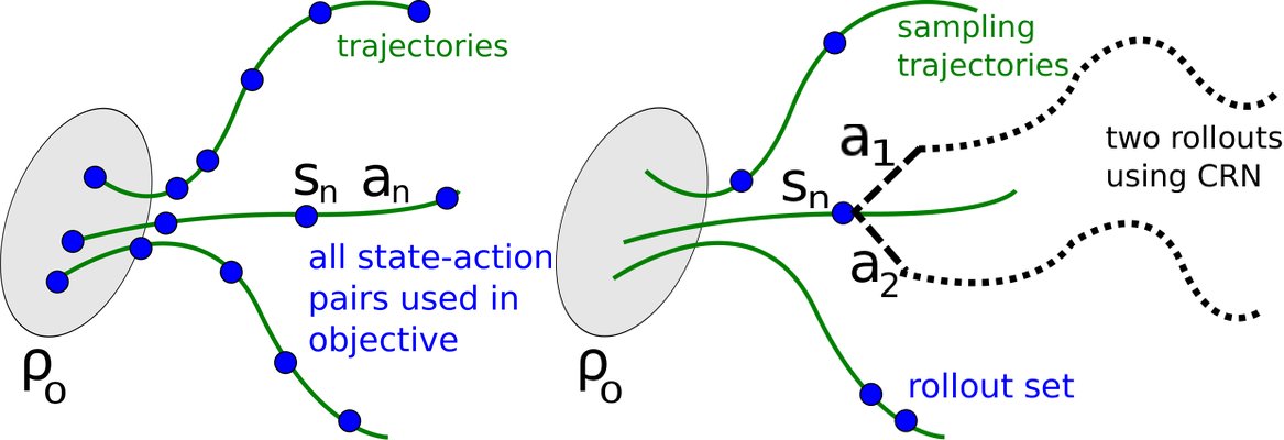
Figure 1: Left: illustration of single path procedure. Here, we generate a set of trajectories via simulation of the policy and incorporate all state-action pairs () into the objective. Right: illustration of vine procedure. We generate a set of “trunk” trajectories, and then generate “branch” rollouts from a subset of the reached states. For each of these states , we perform multiple actions ( and here) and perform a rollout after each action, using common random numbers (CRN) to reduce the variance.
图 1:左:single path 流程示意。通过策略仿真生成一组轨迹,把全部状态—动作对 纳入目标。右:vine 流程示意。先生成一组「主干」轨迹,再从到达状态的子集生成「分支」rollout。对其中每个状态 ,执行多个动作(此处为 与 ),并在每个动作后做 rollout;使用公共随机数(CRN)以降方差。
In this estimation procedure, we first sample and simulate the policy to generate a number of trajectories. We then choose a subset of states along these trajectories, denoted , which we call the “rollout set”. For each state in the rollout set, we sample actions according to . Any choice of with a support that includes the support of will produce a consistent estimator. In practice, we found that works well on continuous problems, such as robotic locomotion, while the uniform distribution works well on discrete tasks, such as the Atari games, where it can sometimes achieve better exploration.
该估计流程中,先采样 并仿真策略 生成若干轨迹。再沿这些轨迹选取 个状态的子集,记为 ,称为「rollout 集合」。对集合中每个状态 ,按 采样 个动作。只要 的支撑包含 的支撑,就能得到相合估计。实践中发现,连续问题(如机器人运动)上 效果好;离散任务(如 Atari)上均匀分布效果好,有时还能带来更好的探索。
For each action sampled at each state , we estimate by performing a rollout (i.e., a short trajectory) starting with state and action . We can greatly reduce the variance of the -value differences between rollouts by using the same random number sequence for the noise in each of the rollouts, i.e., common random numbers. See (Bertsekas 2005) for additional discussion on Monte Carlo estimation of -values and (Ng & Jordan 2000) for a discussion of common random numbers in reinforcement learning.
对每个状态 上采样的每个动作 ,从状态 、动作 出发做一次 rollout(短轨迹),以估计 。若各次 次 rollout 的噪声使用同一随机数序列,即 公共随机数,可大幅降低 rollout 之间 值差的方差。关于 值的蒙特卡洛估计另见 Bertsekas 2005;强化学习中公共随机数的讨论见 Ng & Jordan 2000。
In small, finite action spaces, we can generate a rollout for every possible action from a given state. The contribution to from a single state is as follows:
在小的有限动作空间中,可从给定状态对每个可能动作各做一次 rollout。单个状态 对 的贡献如下:
where the action space is . In large or continuous state spaces, we can construct an estimator of the surrogate objective using importance sampling. The self-normalized estimator (Owen 2013, Chapter 9) of obtained at a single state is
其中动作空间为 。在大或连续状态空间中,可用重要性采样构造代理目标的估计。在单个状态 上得到的 自归一化估计(Owen 2013,第 9 章)为
assuming that we performed actions from state . This self-normalized estimator removes the need to use a baseline for the -values (note that the gradient is unchanged by adding a constant to the -values). Averaging over , we obtain an estimator for , as well as its gradient.
假定我们从状态 执行了 个动作 。该自归一化估计无需再为 值使用基线(注意给 值加常数不改变梯度)。对 取平均,即得到 及其梯度的估计。
The vine and single path methods are illustrated in Figure 1. We use the term vine, since the trajectories used for sampling can be likened to the stems of vines, which branch at various points (the rollout set) into several short offshoots (the rollout trajectories).
vine 与 single path 方法如图 1 所示。我们使用 vine 一词,因为采样所用轨迹可比作藤蔓主干,在若干点(rollout 集合)分出多条短枝(rollout 轨迹)。
The benefit of the vine method over the single path method that is our local estimate of the objective has much lower variance given the same number of -value samples in the surrogate objective. That is, the vine method gives much better estimates of the advantage values. The downside of the vine method is that we must perform far more calls to the simulator for each of these advantage estimates. Furthermore, the vine method requires us to generate multiple trajectories from each state in the rollout set, which limits this algorithm to settings where the system can be reset to an arbitrary state. In contrast, the single path algorithm requires no state resets and can be directly implemented on a physical system (Peters & Schaal 2008b).
vine 相对 single path 的好处是:在代理目标中给定同样数量的 值样本时,目标的局部估计方差低得多,即 vine 对优势值的估计好得多。代价是:每次优势估计要对仿真器调用远为多次;此外 vine 要求从 rollout 集合中每个状态生成多条轨迹,从而把算法限制在系统可重置到任意状态的设定。相比之下,single path 无需状态重置,可直接在物理系统上实现(Peters & Schaal 2008b)。
6 Practical Algorithm
6 实用算法
Here we present two practical policy optimization algorithm based on the ideas above, which use either the single path or vine sampling scheme from the preceding section. The algorithms repeatedly perform the following steps:
此处给出基于上述思想的两种实用策略优化算法,分别使用上一节的 single path 或 vine 采样方案。算法反复执行下列步骤:
- Use the single path or vine procedures to collect a set of state-action pairs along with Monte Carlo estimates of their -values.
- By averaging over samples, construct the estimated objective and constraint in Equation 14.
- Approximately solve this constrained optimization problem to update the policy’s parameter vector . We use the conjugate gradient algorithm followed by a line search, which is altogether only slightly more expensive than computing the gradient itself. See Appendix C for details.
- 用 single path 或 vine 流程收集一组状态—动作对及其 值的蒙特卡洛估计。
- 对样本取平均,构造式 14 中的估计目标与约束。
- 近似求解该约束优化问题以更新策略参数向量 。我们使用共轭梯度再接线搜索,整体代价仅略高于计算梯度本身。细节见附录 C。
With regard to (3), we construct the Fisher information matrix (FIM) by analytically computing the Hessian of the KL divergence, rather than using the covariance matrix of the gradients. That is, we estimate as , rather than . The analytic estimator integrates over the action at each state , and does not depend on the action that was sampled. As described in Appendix C, this analytic estimator has computational benefits in the large-scale setting, since it removes the need to store a dense Hessian or all policy gradients from a batch of trajectories. The rate of improvement in the policy is similar to the empirical FIM, as shown in the experiments.
关于第 (3) 步,我们通过解析计算 KL 散度的 Hessian 来构造 Fisher 信息矩阵(FIM),而不是用梯度的协方差矩阵。也即,把 估计为 ,而非 。解析估计在每个状态 上对动作积分,不依赖所采动作 。如附录 C 所述,大规模设定下该解析估计有计算优势:无需存储稠密 Hessian,也无需存下一批轨迹的全部策略梯度。实验表明,策略改进速率与经验 FIM 相近。
Let us briefly summarize the relationship between the theory from Section 3 and the practical algorithm we have described:
简要总结第 3 节理论与上述实用算法之间的关系:
- • The theory justifies optimizing a surrogate objective with a penalty on KL divergence. However, the large penalty coefficient leads to prohibitively small steps, so we would like to decrease this coefficient. Empirically, it is hard to robustly choose the penalty coefficient, so we use a hard constraint instead of a penalty, with parameter (the bound on KL divergence).
- • The constraint on is hard for numerical optimization and estimation, so instead we constrain .
- • Our theory ignores estimation error for the advantage function. Kakade & Langford 2002 consider this error in their derivation, and the same arguments would hold in the setting of this paper, but we omit them for simplicity.
- • 理论支持优化带 KL 散度惩罚的代理目标。但惩罚系数 过大导致步长过小,我们希望减小该系数。经验上很难稳健地选惩罚系数,因此改用硬约束,参数为 (KL 散度上界)。
- • 对 的约束在数值优化与估计上都很难,因此改为约束 。
- • 我们的理论忽略了优势函数的估计误差。Kakade & Langford 2002 在推导中考虑了该误差,同样论证适用于本文设定,但为简洁起见我们省略。
7 Connections with Prior Work
7 与先前工作的联系
As mentioned in Section 4, our derivation results in a policy update that is related to several prior methods, providing a unifying perspective on a number of policy update schemes. The natural policy gradient (Kakade 2002) can be obtained as a special case of the update in Equation (12) by using a linear approximation to and a quadratic approximation to the constraint, resulting in the following problem:
如第 4 节所述,我们的推导得到的策略更新与若干先前方法相关,从而对多种策略更新方案给出统一视角。自然策略梯度(Kakade 2002)可视为式 (12) 更新的特例:对 做线性近似、对 约束做二次近似,得到如下问题:
The update is , where the stepsize is typically treated as an algorithm parameter. This differs from our approach, which enforces the constraint at each update. Though this difference might seem subtle, our experiments demonstrate that it significantly improves the algorithm’s performance on larger problems.
更新为 ,其中步长 通常当作算法参数。这与我们在每次更新都强制约束的做法不同。差异看似细微,但实验表明它在较大问题上显著提升算法表现。
We can also obtain the standard policy gradient update by using an constraint or penalty:
也可通过对 约束或惩罚得到标准策略梯度更新:
The policy iteration update can also be obtained by solving the unconstrained problem , using as defined in Equation 3.
策略迭代更新也可通过对无约束问题 求解得到,其中 由式 3 定义。
Several other methods employ an update similar to Equation (12). Relative entropy policy search (REPS) (Peters et al. 2010) constrains the state-action marginals , while TRPO constrains the conditionals . Unlike REPS, our approach does not require a costly nonlinear optimization in the inner loop. Levine and Abbeel (Levine & Abbeel 2014) also use a KL divergence constraint, but its purpose is to encourage the policy not to stray from regions where the estimated dynamics model is valid, while we do not attempt to estimate the system dynamics explicitly. Pirotta et al. 2013 also build on and generalize Kakade and Langford’s results, and they derive different algorithms from the ones here.
另有若干方法采用类似式 (12) 的更新。相对熵策略搜索(REPS)(Peters et al. 2010)约束状态—动作边缘 ,而 TRPO 约束条件分布 。与 REPS 不同,我们的方法不要求内层做代价高昂的非线性优化。Levine 与 Abbeel(Levine & Abbeel 2014)也使用 KL 散度约束,但其目的是鼓励策略不要离开估计动力学模型仍有效的区域,而我们并不试图显式估计系统动力学。Pirotta et al. 2013 也建立并推广了 Kakade 与 Langford 的结果,并导出与本文不同的算法。
8 Experiments
8 实验
We designed our experiments to investigate the following questions:
我们设计实验以考察下列问题:
- What are the performance characteristics of the single path and vine sampling procedures?
- TRPO is related to prior methods (e.g. natural policy gradient) but makes several changes, most notably by using a fixed KL divergence rather than a fixed penalty coefficient. How does this affect the performance of the algorithm?
- Can TRPO be used to solve challenging large-scale problems? How does TRPO compare with other methods when applied to large-scale problems, with regard to final performance, computation time, and sample complexity?
- single path 与 vine 采样流程的性能特征如何?
- TRPO 与先前方法(如自然策略梯度)相关,但做了若干改动,最显著的是用固定 KL 散度约束代替固定惩罚系数。这如何影响算法表现?
- TRPO 能否解决具有挑战性的大规模问题?在大规模问题上,TRPO 相对其他方法在最终性能、计算时间与样本复杂度上如何比较?
To answer (1) and (2), we compare the performance of the single path and vine variants of TRPO, several ablated variants, and a number of prior policy optimization algorithms. With regard to (3), we show that both the single path and vine algorithm can obtain high-quality locomotion controllers from scratch, which is considered to be a hard problem. We also show that these algorithms produce competitive results when learning policies for playing Atari games from images using convolutional neural networks with tens of thousands of parameters.
为回答 (1) 与 (2),我们比较 TRPO 的 single path 与 vine 变体、若干消融变体,以及一批先前策略优化算法。关于 (3),我们表明 single path 与 vine 都能从零得到高质量运动控制器——这被认为是难题;也表明在用带数万参数的卷积神经网络从图像学习 Atari 策略时,这些算法能给出有竞争力的结果。
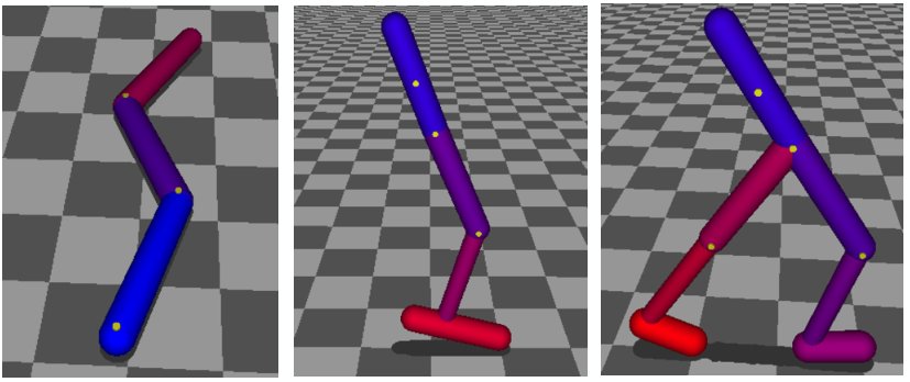
Figure 2: 2D robot models used for locomotion experiments. From left to right: swimmer, hopper, walker. The hopper and walker present a particular challenge, due to underactuation and contact discontinuities.
图 2:运动实验所用的二维机器人模型。从左到右:swimmer、hopper、walker。hopper 与 walker 因欠驱动与接触不连续而特别具有挑战性。
8.1 Simulated Robotic Locomotion
8.1 仿真机器人运动
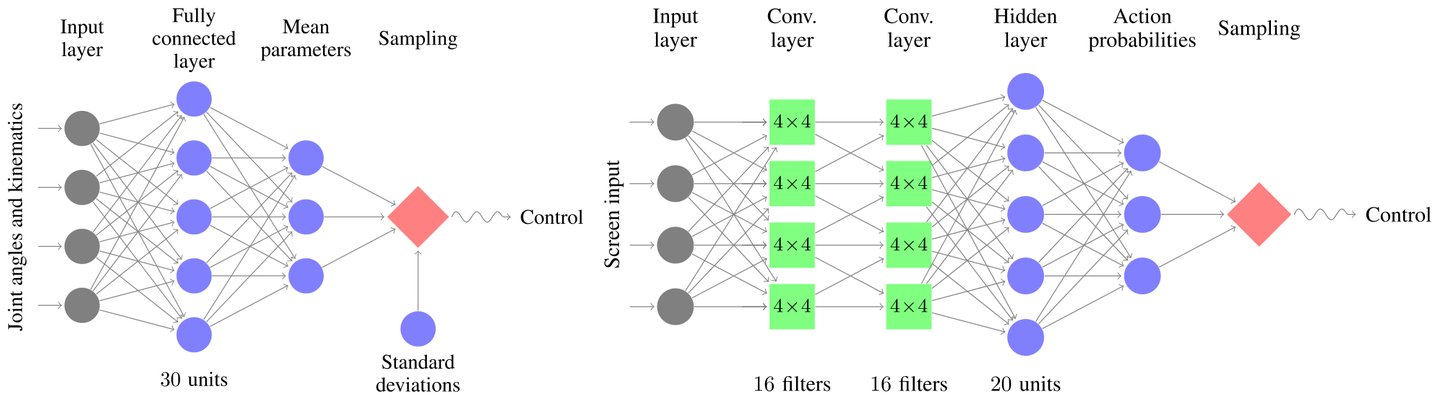
Figure 3: Neural networks used for the locomotion task (top) and for playing Atari games (bottom).
图 3:用于运动任务(上)与玩 Atari 游戏(下)的神经网络。
We conducted the robotic locomotion experiments using the MuJoCo simulator (Todorov et al. 2012). The three simulated robots are shown in Figure 2. The states of the robots are their generalized positions and velocities, and the controls are joint torques. Underactuation, high dimensionality, and non-smooth dynamics due to contacts make these tasks very challenging. The following models are included in our evaluation:
机器人运动实验在 MuJoCo 仿真器中进行(Todorov et al. 2012)。三台仿真机器人见图 2。状态为广义位置与速度,控制为关节力矩。欠驱动、高维以及接触带来的非光滑动力学使这些任务非常困难。评估包含下列模型:
- Swimmer. -dimensional state space, linear reward for forward progress and a quadratic penalty on joint effort to produce the reward . The swimmer can propel itself forward by making an undulating motion.
- Hopper. -dimensional state space, same reward as the swimmer, with a bonus of for being in a non-terminal state. We ended the episodes when the hopper fell over, which was defined by thresholds on the torso height and angle.
- Walker. -dimensional state space. For the walker, we added a penalty for strong impacts of the feet against the ground to encourage a smooth walk rather than a hopping gait.
- Swimmer。 维状态空间;前进进度的线性奖励与关节力矩的二次惩罚,奖励为 。游泳者可通过波动推进自身。
- Hopper。 维状态空间;奖励与游泳者相同,非终止状态另有 奖励。当 hopper 摔倒(由躯干高度与角度阈值定义)时结束回合。
- Walker。 维状态空间。对足部与地面的强冲击额外惩罚,以鼓励平滑行走而非跳跃步态。
We used for all experiments. See Table 2 in the Appendix for more details on the experimental setup and parameters used. We used neural networks to represent the policy, with the architecture shown in Figure 3, and further details provided in Appendix D. To establish a standard baseline, we also included the classic cart-pole balancing problem, based on the formulation from Barto et al. 1983, using a linear policy with six parameters that is easy to optimize with derivative-free black-box optimization methods.
全部实验取 。实验设置与参数细节见附录表 2。策略用图 3 所示神经网络表示,更多细节见附录 D。为建立标准基线,我们还纳入经典倒立摆平衡问题(基于 Barto et al. 1983 的表述),使用仅六参数的线性策略,便于无导数黑箱优化方法优化。
The following algorithms were considered in the comparison: single path TRPO; vine TRPO; cross-entropy method (CEM), a gradient-free method (Szita & Lörincz 2006); covariance matrix adaption (CMA), another gradient-free method (Hansen & Ostermeier 1996); natural gradient, the classic natural policy gradient algorithm (Kakade 2002), which differs from single path by the use of a fixed penalty coefficient (Lagrange multiplier) instead of the KL divergence constraint; empirical FIM, identical to single path, except that the FIM is estimated using the covariance matrix of the gradients rather than the analytic estimate; max KL, which was only tractable on the cart-pole problem, and uses the maximum KL divergence in Equation (11), rather than the average divergence, allowing us to evaluate the quality of this approximation. The parameters used in the experiments are provided in Appendix E. For the natural gradient method, we swept through the possible values of the stepsize in factors of three, and took the best value according to the final performance.
比较中考虑下列算法:single path TRPO;vine TRPO;交叉熵方法(CEM),无梯度方法(Szita & Lörincz 2006);协方差矩阵自适应(CMA),另一无梯度方法(Hansen & Ostermeier 1996);自然梯度,经典自然策略梯度算法(Kakade 2002),与 single path 的差别在于使用固定惩罚系数(拉格朗日乘子)而非 KL 散度约束;经验 FIM,与 single path 相同,但 FIM 用梯度协方差矩阵估计而非解析估计;max KL,仅在倒立摆问题上可解,使用式 (11) 的最大 KL 散度而非平均散度,以便评估该近似的质量。实验参数见附录 E。对 自然梯度 方法,我们按三倍因子扫过可能步长,并按最终性能取最佳值。

Figure 4: Learning curves for locomotion tasks, averaged across five runs of each algorithm with random initializations. Note that for the hopper and walker, a score of is achievable without any forward velocity, indicating a policy that simply learned balanced standing, but not walking.
图 4:运动任务学习曲线,每种算法五次随机初始化运行的平均。注意对 hopper 与 walker,分数 在无任何前进速度时即可达到,表示策略只学会了平衡站立而未学会行走。
Learning curves showing the total reward averaged across five runs of each algorithm are shown in Figure 4. Single path and vine TRPO solved all of the problems, yielding the best solutions. Natural gradient performed well on the two easier problems, but was unable to generate hopping and walking gaits that made forward progress. These results provide empirical evidence that constraining the KL divergence is a more robust way to choose step sizes and make fast, consistent progress, compared to using a fixed penalty. CEM and CMA are derivative-free algorithms, hence their sample complexity scales unfavorably with the number of parameters, and they performed poorly on the larger problems. The max KL method learned somewhat more slowly than our final method, due to the more restrictive form of the constraint, but overall the result suggests that the average KL divergence constraint has a similar effect as the theorecally justified maximum KL divergence. Videos of the policies learned by TRPO may be viewed on the project website: http://sites.google.com/site/trpopaper/.
图 4 给出每种算法五次运行平均的总奖励学习曲线。Single path 与 vine TRPO 解决了全部问题,并给出最佳解。自然梯度 在两个较易问题上表现良好,但无法生成有前进进度的跳跃与行走步态。这些结果经验表明:约束 KL 散度比使用固定惩罚更能稳健地选择步长并快速、一致地进步。CEM 与 CMA 是无导数算法,样本复杂度随参数量不利地增长,在较大问题上表现差。max KL 方法因约束形式更严而学得略慢,但总体结果表明平均 KL 散度约束与理论支持的最大 KL 散度作用相近。TRPO 学到的策略视频见项目网站:http://sites.google.com/site/trpopaper/。
Note that TRPO learned all of the gaits with general-purpose policies and simple reward functions, using minimal prior knowledge. This is in contrast with most prior methods for learning locomotion, which typically rely on hand-architected policy classes that explicitly encode notions of balance and stepping (Tedrake et al. 2004; Geng et al. 2006; Wampler & Popović 2009).
注意 TRPO 用通用策略与简单奖励函数、极少先验知识就学会了全部步态。这与多数先前运动学习方法形成对比——后者通常依赖显式编码平衡与迈步概念的手工策略类(Tedrake et al. 2004;Geng et al. 2006;Wampler & Popović 2009)。
| B. Rider | Breakout | Enduro | Pong | Qbert* | Seaquest | S. Invaders | |
|---|---|---|---|---|---|---|---|
| Random | 354 | 1.2 | 0 | 157 | 110 | 179 | |
| Human (Mnih et al. 2013) | 7456 | 31.0 | 368 | 18900 | 28010 | 3690 | |
| Deep Q Learning (Mnih et al. 2013) | 4092 | 168.0 | 470 | 20.0 | 1952 | 1705 | 581 |
| UCC-I (Guo et al. 2014) | 5702 | 380 | 741 | 21 | 20025 | 2995 | 692 |
| TRPO - single path | 1425.2 | 10.8 | 534.6 | 20.9 | 1973.5 | 1908.6 | 568.4 |
| TRPO - vine | 859.5 | 34.2 | 430.8 | 20.9 | 7732.5 | 788.4 | 450.2 |
Table 1: Performance comparison for vision-based RL algorithms on the Atari domain. Our algorithms (bottom rows) were run once on each task, with the same architecture and parameters. Performance varies substantially from run to run (with different random initializations of the policy), but we could not obtain error statistics due to time constraints.
| B. Rider | Breakout | Enduro | Pong | Qbert* | Seaquest | S. Invaders | |
|---|---|---|---|---|---|---|---|
| Random | 354 | 1.2 | 0 | 157 | 110 | 179 | |
| Human (Mnih et al. 2013) | 7456 | 31.0 | 368 | 18900 | 28010 | 3690 | |
| Deep Q Learning (Mnih et al. 2013) | 4092 | 168.0 | 470 | 20.0 | 1952 | 1705 | 581 |
| UCC-I (Guo et al. 2014) | 5702 | 380 | 741 | 21 | 20025 | 2995 | 692 |
| TRPO - single path | 1425.2 | 10.8 | 534.6 | 20.9 | 1973.5 | 1908.6 | 568.4 |
| TRPO - vine | 859.5 | 34.2 | 430.8 | 20.9 | 7732.5 | 788.4 | 450.2 |
表 1:Atari 域上基于视觉的 RL 算法性能比较。我们的算法(底两行)在每项任务上各跑一次,架构与参数相同。不同随机初始化下性能波动很大,但因时间限制未能获得误差统计。
8.2 Playing Games from Images
8.2 从图像玩游戏
To evaluate TRPO on a partially observed task with complex observations, we trained policies for playing Atari games, using raw images as input. The games require learning a variety of behaviors, such as dodging bullets and hitting balls with paddles. Aside from the high dimensionality, challenging elements of these games include delayed rewards (no immediate penalty is incurred when a life is lost in Breakout or Space Invaders); complex sequences of behavior (Q*bert requires a character to hop on different platforms); and non-stationary image statistics (Enduro involves a changing and flickering background).
为在具有复杂观测的部分可观测任务上评估 TRPO,我们以原始图像为输入训练玩 Atari 的策略。这些游戏需要学会多种行为,如躲避子弹、用挡板击球。除高维外,挑战还包括延迟奖励(Breakout 或 Space Invaders 丢命时无即时惩罚)、复杂行为序列(Q*bert 要求角色跳上 个不同平台),以及非平稳图像统计(Enduro 背景变化且闪烁)。
We tested our algorithms on the same seven games reported on in (Mnih et al. 2013) and (Guo et al. 2014), which are made available through the Arcade Learning Environment (Bellemare et al. 2013) The images were preprocessed following the protocol in Mnih et al (Mnih et al. 2013), and the policy was represented by the convolutional neural network shown in Figure 3, with two convolutional layers with channels and stride , followed by one fully-connected layer with units, yielding 33,500 parameters.
我们在 (Mnih et al. 2013) 与 (Guo et al. 2014) 所报的同一七款游戏上测试,游戏由 Arcade Learning Environment 提供(Bellemare et al. 2013)。图像预处理遵循 Mnih et al.(Mnih et al. 2013)的协议;策略由图 3 所示卷积神经网络表示:两个 通道、步长 的卷积层,再接一个 单元全连接层,共 33,500 个参数。
The results of the vine and single path algorithms are summarized in Table 1, which also includes an expert human performance and two recent methods: deep -learning (Mnih et al. 2013), and a combination of Monte-Carlo Tree Search with supervised training (Guo et al. 2014), called UCC-I. The 500 iterations of our algorithm took about 30 hours (with slight variation between games) on a 16-core computer. While our method only outperformed the prior methods on some of the games, it consistently achieved reasonable scores. Unlike the prior methods, our approach was not designed specifically for this task. The ability to apply the same policy search method to methods as diverse as robotic locomotion and image-based game playing demonstrates the generality of TRPO.
vine 与 single path 算法的结果汇总于表 1,表中还包含专家人类表现以及两种近期方法:深度 学习(Mnih et al. 2013),以及蒙特卡洛树搜索与监督训练的结合(Guo et al. 2014),称为 UCC-I。算法运行 500 次迭代约需 30 小时(游戏间略有差异),在 16 核计算机上完成。我们的方法仅在部分游戏上超过先前方法,但始终达到合理分数。与先前方法不同,我们的方法并非专为该任务设计。能把同一策略搜索方法用于机器人运动与基于图像的游戏如此多样的问题,说明了 TRPO 的通用性。
9 Discussion
9 讨论
We proposed and analyzed trust region methods for optimizing stochastic control policies. We proved monotonic improvement for an algorithm that repeatedly optimizes a local approximation to the expected return of the policy with a KL divergence penalty, and we showed that an approximation to this method that incorporates a KL divergence constraint achieves good empirical results on a range of challenging policy learning tasks, outperforming prior methods. Our analysis also provides a perspective that unifies policy gradient and policy iteration methods, and shows them to be special limiting cases of an algorithm that optimizes a certain objective subject to a trust region constraint.
我们提出并分析了用于优化随机控制策略的信赖域方法。我们证明:反复优化带 KL 散度惩罚的策略期望回报局部近似的算法具有单调改进;并表明对该方法做带 KL 散度约束的近似,能在一系列有挑战性的策略学习任务上取得良好经验结果,超过先前方法。我们的分析也提供了统一策略梯度与策略迭代的视角,表明它们是在信赖域约束下优化某一目标的算法的特殊极限情形。
In the domain of robotic locomotion, we successfully learned controllers for swimming, walking and hopping in a physics simulator, using general purpose neural networks and minimally informative rewards. To our knowledge, no prior work has learned controllers from scratch for all of these tasks, using a generic policy search method and non-engineered, general-purpose policy representations. In the game-playing domain, we learned convolutional neural network policies that used raw images as inputs. This requires optimizing extremely high-dimensional policies, and only two prior methods report successful results on this task.
在机器人运动领域,我们在物理仿真器中用通用神经网络与信息量极少的奖励,成功学会了游泳、行走与跳跃的控制器。据我们所知,此前尚无工作用通用策略搜索方法与非工程化的通用策略表示,从零学会所有这些任务的控制器。在游戏领域,我们学会了以原始图像为输入的卷积神经网络策略。这要求优化极高维策略,此前仅有两种方法报告在该任务上成功。
Since the method we proposed is scalable and has strong theoretical foundations, we hope that it will serve as a jumping-off point for future work on training large, rich function approximators for a range of challenging problems. At the intersection of the two experimental domains we explored, there is the possibility of learning robotic control policies that use vision and raw sensory data as input, providing a unified scheme for training robotic controllers that perform both perception and control. The use of more sophisticated policies, including recurrent policies with hidden state, could further make it possible to roll state estimation and control into the same policy in the partially-observed setting. By combining our method with model learning, it would also be possible to substantially reduce its sample complexity, making it applicable to real-world settings where samples are expensive.
由于所提方法可扩展且有坚实理论基础,我们希望它能成为未来在一系列挑战性问题上训练大型、丰富函数逼近器的起点。在我们探索的两个实验域交汇处,有可能学习以视觉与原始感官数据为输入的机器人控制策略,从而给出同时完成感知与控制的统一训练方案。使用更复杂的策略(包括带隐状态的循环策略)可进一步使部分可观测设定下把状态估计与控制卷入同一策略成为可能。把我们的方法与模型学习结合,也可大幅降低样本复杂度,使其适用于样本昂贵的真实世界设定。
Acknowledgements
致谢
We thank Emo Todorov and Yuval Tassa for providing the MuJoCo simulator; Bruno Scherrer, Tom Erez, Greg Wayne, and the anonymous ICML reviewers for insightful comments, and Vitchyr Pong and Shane Gu for pointing our errors in a previous version of the manuscript. This research was funded in part by the Office of Naval Research through a Young Investigator Award and under grant number N00014-11-1-0688, DARPA through a Young Faculty Award, by the Army Research Office through the MAST program.
感谢 Emo Todorov 与 Yuval Tassa 提供 MuJoCo 仿真器;感谢 Bruno Scherrer、Tom Erez、Greg Wayne 以及匿名 ICML 审稿人的深刻评论;感谢 Vitchyr Pong 与 Shane Gu 指出手稿先前版本中的错误。本研究部分由海军研究办公室通过青年研究者奖及资助号 N00014-11-1-0688 资助,由 DARPA 通过青年教师奖资助,并由陆军研究办公室通过 MAST 项目资助。
References
参考文献
Bagnell & Schneider (2003) Bagnell, J. A. and Schneider, J. Covariant policy search. IJCAI, 2003.
Bartlett & Baxter (2011) Bartlett, P. L. and Baxter, J. Infinite-horizon policy-gradient estimation. arXiv preprint arXiv:1106.0665 , 2011.
Barto et al. (1983) Barto, A., Sutton, R., and Anderson, C. Neuronlike adaptive elements that can solve difficult learning control problems. IEEE Transactions on Systems, Man and Cybernetics , (5):834–846, 1983.
Bellemare et al. (2013) Bellemare, M. G., Naddaf, Y., Veness, J., and Bowling, M. The arcade learning environment: An evaluation platform for general agents. Journal of Artificial Intelligence Research , 47:253–279, jun 2013.
Bertsekas (2005) Bertsekas, D. Dynamic programming and optimal control , volume 1. 2005.
Deisenroth et al. (2013) Deisenroth, M., Neumann, G., and Peters, J. A survey on policy search for robotics. Foundations and Trends in Robotics , 2(1-2):1–142, 2013.
Gabillon et al. (2013) Gabillon, Victor, Ghavamzadeh, Mohammad, and Scherrer, Bruno. Approximate dynamic programming finally performs well in the game of Tetris. In Advances in Neural Information Processing Systems , 2013.
Geng et al. (2006) Geng, T., Porr, B., and Wörgötter, F. Fast biped walking with a reflexive controller and realtime policy searching. In Advances in Neural Information Processing Systems (NIPS) , 2006.
Guo et al. (2014) Guo, X., Singh, S., Lee, H., Lewis, R. L., and Wang, X. Deep learning for real-time atari game play using offline Monte-Carlo tree search planning. In Advances in Neural Information Processing Systems , pp. 3338–3346, 2014.
Hansen & Ostermeier (1996) Hansen, Nikolaus and Ostermeier, Andreas. Adapting arbitrary normal mutation distributions in evolution strategies: The covariance matrix adaptation. In Evolutionary Computation, 1996., Proceedings of IEEE International Conference on , pp. 312–317. IEEE, 1996.
Hunter & Lange (2004) Hunter, David R and Lange, Kenneth. A tutorial on MM algorithms. The American Statistician , 58(1):30–37, 2004.
Kakade (2002) Kakade, Sham. A natural policy gradient. In Advances in Neural Information Processing Systems , pp. 1057–1063. MIT Press, 2002.
Kakade & Langford (2002) Kakade, Sham and Langford, John. Approximately optimal approximate reinforcement learning. In ICML , volume 2, pp. 267–274, 2002.
Lagoudakis & Parr (2003) Lagoudakis, Michail G and Parr, Ronald. Reinforcement learning as classification: Leveraging modern classifiers. In ICML , volume 3, pp. 424–431, 2003.
Levin et al. (2009) Levin, D. A., Peres, Y., and Wilmer, E. L. Markov chains and mixing times . American Mathematical Society, 2009.
Levine & Abbeel (2014) Levine, Sergey and Abbeel, Pieter. Learning neural network policies with guided policy search under unknown dynamics. In Advances in Neural Information Processing Systems , pp. 1071–1079, 2014.
Martens & Sutskever (2012) Martens, J. and Sutskever, I. Training deep and recurrent networks with hessian-free optimization. In Neural Networks: Tricks of the Trade , pp. 479–535. Springer, 2012.
Mnih et al. (2013) Mnih, V., Kavukcuoglu, K., Silver, D., Graves, A., Antonoglou, I., Wierstra, D., and Riedmiller, M. Playing Atari with deep reinforcement learning. arXiv preprint arXiv:1312.5602 , 2013.
Nemirovski (2005) Nemirovski, Arkadi. Efficient methods in convex programming. 2005.
Ng & Jordan (2000) Ng, A. Y. and Jordan, M. PEGASUS: A policy search method for large mdps and pomdps. In Uncertainty in artificial intelligence (UAI) , 2000.
Owen (2013) Owen, Art B. Monte Carlo theory, methods and examples . 2013.
Pascanu & Bengio (2013) Pascanu, Razvan and Bengio, Yoshua. Revisiting natural gradient for deep networks. arXiv preprint arXiv:1301.3584 , 2013.
Peters & Schaal (2008a) Peters, J. and Schaal, S. Reinforcement learning of motor skills with policy gradients. Neural Networks , 21(4):682–697, 2008a.
Peters et al. (2010) Peters, J., Mülling, K., and Altün, Y. Relative entropy policy search. In AAAI Conference on Artificial Intelligence , 2010.
Peters & Schaal (2008b) Peters, Jan and Schaal, Stefan. Natural actor-critic. Neurocomputing , 71(7):1180–1190, 2008b.
Pirotta et al. (2013) Pirotta, Matteo, Restelli, Marcello, Pecorino, Alessio, and Calandriello, Daniele. Safe policy iteration. In Proceedings of The 30th International Conference on Machine Learning , pp. 307–315, 2013.
Pollard (2000) Pollard, David. Asymptopia: an exposition of statistical asymptotic theory . 2000. URL http://www.stat.yale.edu/~pollard/Books/Asymptopia .
Szita & Lörincz (2006) Szita, István and Lörincz, András. Learning tetris using the noisy cross-entropy method. Neural computation , 18(12):2936–2941, 2006.
Tedrake et al. (2004) Tedrake, R., Zhang, T., and Seung, H. Stochastic policy gradient reinforcement learning on a simple 3d biped. In IEEE/RSJ International Conference on Intelligent Robots and Systems , 2004.
Todorov et al. (2012) Todorov, Emanuel, Erez, Tom, and Tassa, Yuval. MuJoCo: A physics engine for model-based control. In Intelligent Robots and Systems (IROS), 2012 IEEE/RSJ International Conference on , pp. 5026–5033. IEEE, 2012.
Wampler & Popović (2009) Wampler, Kevin and Popović, Zoran. Optimal gait and form for animal locomotion. In ACM Transactions on Graphics (TOG) , volume 28, pp. 60. ACM, 2009.
Wright & Nocedal (1999) Wright, Stephen J and Nocedal, Jorge. Numerical optimization , volume 2. Springer New York, 1999.
Appendix A Proof of Policy Improvement Bound
附录 A 策略改进界的证明
This proof (of 1) uses techniques from the proof of Theorem 4.1 in (Kakade & Langford 2002), adapting them to the more general setting considered in this paper. An informal overview is as follows. Our proof relies on the notion of coupling, where we jointly define the policies and so that they choose the same action with high probability . Surrogate loss accounts for the the advantage of the first time that it disagrees with , but not subsequent disagreements. Hence, the error in is due to two or more disagreements between and , hence, we get an correction term, where is the probability of disagreement.
本证明(定理 1)采用 (Kakade & Langford 2002) 中定理 4.1 证明的技巧,并适配到本文考虑的更一般设定。非正式概览如下。证明依赖耦合:我们联合定义策略 与 ,使它们以高概率 选择同一动作。代理损失 计入 第一次与 不一致时的优势,但不计入后续不一致。因此 的误差来自 与 的两次或更多次不一致,从而得到 修正项,其中 为不一致概率。
We start out with a lemma from Kakade & Langford 2002 that shows that the difference in policy performance can be decomposed as a sum of per-timestep advantages.
我们从 Kakade & Langford 2002 的一条引理出发:它表明策略性能差 可分解为逐步优势之和。
Lemma 1.
Given two policies ,
引理 1。
给定两策略 ,
This expectation is taken over trajectories , and the notation indicates that actions are sampled from to generate .
期望对轨迹 取;记号 表示动作用 采样以生成 。
Proof.
First note that . Therefore,
证明。
首先注意 。因此,
Rearranging, the result follows. ∎
整理后即得结论。∎
Define to be the expected advantage of over at state :
定义 为状态 上 相对 的期望优势:
Now Lemma 1 can be written as follows:
于是引理 1 可写成:
Note that can be written as
注意 可写成
The difference in these equations is whether the states are sampled using or . To bound the difference between and , we will bound the difference arising from each timestep. To do this, we first need to introduce a measure of how much and agree. Specifically, we’ll couple the policies, so that they define a joint distribution over pairs of actions.
这些等式的差别在于状态是用 还是 采样。为界住 与 之差,我们界住每个时间步带来的差。为此需先引入衡量 与 一致程度的量。具体地,我们将策略 耦合,使它们定义动作对上的联合分布。
Definition 1.
is an -coupled policy pair if it defines a joint distribution , such that for all . and will denote the marginal distributions of and , respectively.
定义 1。
是 -耦合策略对,若它定义联合分布 ,使得对所有 有 。 与 分别表示 与 的边缘分布。
Computationally, -coupling means that if we randomly choose a seed for our random number generator, and then we sample from each of and after setting that seed, the results will agree for at least fraction of seeds.
从计算角度看,-耦合意味着:若随机选定随机数生成器种子,再在设好该种子后分别从 与 采样,则至少有比例 的种子上结果一致。
Lemma 2.
Given that are -coupled policies, for all ,
引理 2。
给定 为 -耦合策略,则对所有 ,
Proof.
∎
Lemma 3.
Let be an -coupled policy pair. Then
引理 3。
令 为 -耦合策略对。则
Proof.
Given the coupled policy pair , we can also obtain a coupling over the trajectory distributions produced by and , respectively. Namely, we have pairs of trajectories , where is obtained by taking actions from , and is obtained by taking actions from , where the same random seed is used to generate both trajectories. We will consider the advantage of over at timestep , and decompose this expectation based on whether agrees with at all timesteps .
证明。
给定耦合策略对 ,也可得到 与 各自产生的轨迹分布上的耦合。即有轨迹对 : 由 取动作得到, 由 取动作得到,两者用同一随机种子生成。我们考虑时刻 上 相对 的优势,并按 是否在所有 的时间步都与 一致来分解该期望。
Let denote the number of times that for , i.e., the number of times that and disagree before timestep .
令 表示 时 的次数,即时刻 之前 与 不一致的次数。
The expectation decomposes similarly for actions are sampled using :
当动作用 采样时,期望可类似分解:
Note that the terms are equal:
注意 的项相等:
\displaystyle\mathbb{E}_{s_{t}\sim{\color[rgb]{1,0,0}\tilde{\pi}}|n_{t}=0}\left[\bar{A}(s_{t})\right]=\mathbb{E}_{s_{t}\sim{\color[rgb]{1,0,0}\pi}|n_{t}=0}\left[\bar{A}(s_{t})\right], \tag{35}
because indicates that and agreed on all timesteps less than . Subtracting Equations 33 and 34, we get
因为 表示 与 在小于 的所有时间步都一致。式 33 减式 34 得
By definition of , P(\pi,\tilde{\pi}\text{ agree at timestepi})\geq 1-\alpha, so , and
由 的定义,P(\pi,\tilde{\pi}\text{ agree at timestepi})\geq 1-\alpha,故 ,并且
Next, note that
接下来注意
Where the second inequality follows from Lemma 3.
其中第二个不等式由引理 2 得出。(原文写作 Lemma 3,应为引理 2。)
Plugging Equation 37 and Equation 39 into Equation 36, we get
把式 37 与式 39 代入式 36,得
∎
The preceding Lemma bounds the difference in expected advantage at each timestep . We can sum over time to bound the difference between and . Subtracting Equation 26 and Equation 27, and defining ,
上述引理界住了每个时间步 上期望优势的差。对时间求和即可界住 与 之差。式 26 减式 27,并定义 ,
Last, to replace by the total variation divergence, we need to use the correspondence between TV divergence and coupled random variables:
最后,要把 换成全变差散度,需用 TV 散度与耦合随机变量之间的对应:
Suppose and are distributions with . Then there exists a joint distribution whose marginals are , for which with probability .
设分布 与 满足 。则存在边缘分别为 的联合分布 ,使 的概率为 。
See (Levin et al. 2009), Proposition 4.7.
见 (Levin et al. 2009),命题 4.7。
It follows that if we have two policies and such that , then we can define an -coupled policy pair with appropriate marginals. Taking in Equation 45, 1 follows.
因此,若两策略 与 满足 ,则可定义具有相应边缘的 -耦合策略对 。在式 45 中取 ,即得定理 1。
Appendix B Perturbation Theory Proof of Policy Improvement Bound
附录 B 策略改进界的摄动理论证明
We also provide an alternative proof of 1 using perturbation theory.
我们也给出定理 1 的另一证明,使用摄动理论。
Proof.
Let , and similarly Let . We will use the convention that (a density on state space) is a vector and (a reward function on state space) is a dual vector (i.e., linear functional on vectors), thus is a scalar meaning the expected reward under density . Note that , and . Let . We want to bound . We start with some standard perturbation theory manipulations.
证明。
令 ,类似地令 。约定 (状态空间上的密度)为向量,(状态空间上的奖励函数)为对偶向量(即向量上的线性泛函),因而 是标量,表示密度 下的期望奖励。注意 ,(原文写 ,应为 )。令 。我们要界住 。先做若干标准摄动演算。
Left multiply by and right multiply by .
左乘 、右乘 。
Substituting the right-hand side into gives
把右侧代回 得
So we have
于是有
Let us first consider the leading term . Note that , i.e., the infinite-horizon state-value function. Also note that . Thus we can write . We will show that this expression equals the expected advantage .
先看首项 。注意 ,即无限时域状态价值函数;又 。因而可写 。我们将说明该式等于期望优势 。
Next let us bound the term . First we consider the product . Consider the component of this dual vector.
接下来界住 项 。先考虑乘积 。看该对偶向量的分量 。
where the last line used the definition of the total-variation divergence, and the definition of . We bound the other portion using the operator norm
其中末行用了全变差散度的定义以及 。再用 算子范数界住另一部分
where we have that and . That gives
其中 ,。于是
So we have that
于是有
∎
Appendix C Efficiently Solving the Trust-Region Constrained Optimization Problem
附录 C 高效求解信赖域约束优化问题
This section describes how to efficiently approximately solve the following constrained optimization problem, which we must solve at each iteration of TRPO:
本节说明如何高效近似求解下列约束优化问题——TRPO 每次迭代都要求解它:
The method we will describe involves two steps: (1) compute a search direction, using a linear approximation to objective and quadratic approximation to the constraint; and (2) perform a line search in that direction, ensuring that we improve the nonlinear objective while satisfying the nonlinear constraint.
所述方法分两步:(1)用目标的线性近似与约束的二次近似计算搜索方向;(2)沿该方向做线搜索,确保改进非线性目标并满足非线性约束。
The search direction is computed by approximately solving the equation , where is the Fisher information matrix, i.e., the quadratic approximation to the KL divergence constraint: , where . In large-scale problems, it is prohibitively costly (with respect to computation and memory) to form the full matrix (or ). However, the conjugate gradient algorithm allows us to approximately solve the equation without forming this full matrix, when we merely have access to a function that computes matrix-vector products . Section C.1 describes the most efficient way to compute matrix-vector products with the Fisher information matrix. For additional exposition on the use of Hessian-vector products for optimizing neural network objectives, see (Martens & Sutskever 2012) and (Pascanu & Bengio 2013).
搜索方向通过近似求解方程 得到,其中 是 Fisher 信息矩阵,即对 KL 散度约束的二次近似:,其中 。大规模问题中,形成完整矩阵 (或 )在计算与内存上代价过高。但共轭梯度算法允许我们在仅能计算矩阵—向量积 时近似求解 ,而无需形成完整矩阵。第 C.1 节描述计算 Fisher 信息矩阵矩阵—向量积的最高效方式。关于用 Hessian—向量积优化神经网络目标的更多阐述,见 (Martens & Sutskever 2012) 与 (Pascanu & Bengio 2013)。
Having computed the search direction , we next need to compute the maximal step length such that will satisfy the KL divergence constraint. To do this, let . From this, we obtain , where is the desired KL divergence. The term can be computed through a single Hessian vector product, and it is also an intermediate result produced by the conjugate gradient algorithm.
算出搜索方向 后,还需计算最大步长 ,使 满足 KL 散度约束。为此令 。由此得 ,其中 为期望的 KL 散度。项 可通过一次 Hessian—向量积计算,也是共轭梯度算法的中间结果。
Last, we use a line search to ensure improvement of the surrogate objective and satisfaction of the KL divergence constraint, both of which are nonlinear in the parameter vector (and thus depart from the linear and quadratic approximations used to compute the step). We perform the line search on the objective , where equals zero when its argument is true and when it is false. Starting with the maximal value of the step length computed in the previous paragraph, we shrink exponentially until the objective improves. Without this line search, the algorithm occasionally computes large steps that cause a catastrophic degradation of performance.
最后,用线搜索确保代理目标改进并满足 KL 散度约束——二者都对参数向量 非线性(因而偏离了用于计算步长的线性与二次近似)。我们在目标 上做线搜索,其中 在自变量为真时为 0,为假时为 。从上一小节算出的最大步长 出发,指数地缩小 ,直到目标改进。若无线搜索,算法偶尔会算出导致性能灾难性下降的大步。
C.1 Computing the Fisher-Vector Product
C.1 计算 Fisher—向量积
Here we will describe how to compute the matrix-vector product between the averaged Fisher information matrix and arbitrary vectors. This matrix-vector product enables us to perform the conjugate gradient algorithm. Suppose that the parameterized policy maps from the input to “distribution parameter” vector , which parameterizes the distribution . Now the KL divergence for a given input can be written as follows:
此处说明如何计算平均 Fisher 信息矩阵与任意向量的矩阵—向量积。该积使我们能运行共轭梯度算法。假定参数化策略把输入 映射到「分布参数」向量 ,后者参数化分布 。则给定输入 的 KL 散度可写成:
where is the KL divergence between the distributions corresponding to the two mean parameter vectors. Differentiating twice with respect to , we obtain
其中 是对应于两个均值参数向量的分布之间的 KL 散度。对 求 的二阶导,得
where the primes (′) indicate differentiation with respect to the first argument, and there is an implied summation over indices . The second term vanishes, leaving just the first term. Let (the Jacobian), then the Fisher information matrix can be written in matrix form as , where is the Fisher information matrix of the distribution in terms of the mean parameter (as opposed to the parameter ). This has a simple form for most parameterized distributions of interest.
其中撇号(′)表示对第一自变量求导,并对指标 隐含求和。第二项消失,只剩第一项。令 (Jacobian),则 Fisher 信息矩阵可写成矩阵形式 ,其中 是分布关于均值参数 (而非参数 )的 Fisher 信息矩阵。对多数关心的参数化分布,它形式简单。
The Fisher-vector product can now be written as a function . Multiplication by and can be performed by most automatic differentiation and neural network packages (multiplication by is the well-known backprop operation), and the operation for multiplication by can be derived for the distribution of interest. Note that this Fisher-vector product is straightforward to average over a set of datapoints, i.e., inputs to .
Fisher—向量积于是可写成函数 。乘以 与 可由多数自动微分与神经网络软件包完成(乘以 即熟知的反向传播),乘以 的运算可针对所关心的分布推导。注意该 Fisher—向量积很容易对一组数据点(即 的输入 )取平均。
One could alternatively use a generic method for calculating Hessian-vector products using reverse mode automatic differentiation ((Wright & Nocedal 1999), chapter 8), computing the Hessian of with respect to . This method would be slightly less efficient as it does not exploit the fact that the second derivatives of (i.e., the second term in Equation 57) can be ignored, but may be substantially easier to implement.
也可改用反向模式自动微分计算 Hessian—向量积的通用方法((Wright & Nocedal 1999),第 8 章),直接对 求 的 Hessian。该方法稍慢,因未利用 的二阶导(即式 57 第二项)可忽略这一事实,但实现可能容易得多。
We have described a procedure for computing the Fisher-vector product , where the Fisher information matrix is averaged over a set of inputs to the function . Computing the Fisher-vector product is typically about as expensive as computing the gradient of an objective that depends on (Wright & Nocedal 1999). Furthermore, we need to compute of these Fisher-vector products per gradient, where is the number of iterations of the conjugate gradient algorithm we perform. We found to be quite effective, and using higher did not result in faster policy improvement. Hence, a naïve implementation would spend more than of the computational effort on these Fisher-vector products. However, we can greatly reduce this burden by subsampling the data for the computation of Fisher-vector product. Since the Fisher information matrix merely acts as a metric, it can be computed on a subset of the data without severely degrading the quality of the final step. Hence, we can compute it on of the data, and the total cost of Hessian-vector products will be about the same as computing the gradient. With this optimization, the computation of a natural gradient step does not incur a significant extra computational cost beyond computing the gradient .
我们描述了计算 Fisher—向量积 的流程,其中 Fisher 信息矩阵对函数 的一组输入取平均。计算 Fisher—向量积通常与计算依赖 的目标梯度代价相当(Wright & Nocedal 1999)。此外,每个梯度需要计算 次这类 Fisher—向量积,其中 是共轭梯度迭代次数。我们发现 相当有效,更大的 并未带来更快的策略改进。因此,朴素实现会把超过 的计算花在这些 Fisher—向量积上。但可通过子采样用于计算 Fisher—向量积的数据大幅减轻负担。由于 Fisher 信息矩阵只充当度量,可在数据子集上计算而不严重损害最终步的质量。因此可在 的数据上计算,Hessian—向量积的总代价约与计算梯度相当。有了这一优化,计算自然梯度步 相对计算梯度 并不带来显著额外计算代价。
Appendix D Approximating Factored Policies with Neural Networks
附录 D 用神经网络逼近分解策略
The policy, which is a conditional probability distribution , can be parameterized with a neural network. This neural network maps (deterministically) from the state vector to a vector , which specifies a distribution over action space. Then we can compute the likelihood and sample .
策略是条件概率分布 ,可用神经网络参数化。该网络把状态向量 确定性映射到向量 ,后者指定动作空间上的分布。然后可计算似然 并采样 。
For our experiments with continuous state and action spaces, we used a Gaussian distribution, where the covariance matrix was diagonal and independent of the state. A neural network with several fully-connected (dense) layers maps from the input features to the mean of a Gaussian distribution. A separate set of parameters specifies the log standard deviation of each element. More concretely, the parameters include a set of weights and biases for the neural network computing the mean, , and a vector (log standard deviation) with the same dimension as . Then, the policy is defined by the normal distribution . Here, .
对连续状态与动作空间的实验,我们使用高斯分布,协方差矩阵对角且与状态无关。带若干全连接(稠密)层的神经网络把输入特征映射到高斯均值;另有一组参数指定每个元素的对数标准差。更具体地,参数包括计算均值的神经网络权重与偏置 ,以及与 同维的向量 (对数标准差)。策略由正态分布 定义。此处 。
For the experiments with discrete actions (Atari), we use a factored discrete action space, where each factor is parameterized as a categorical distribution. That is, the action consists of a tuple of integers , and each of these components is assumed to have a categorical distribution, which is specified by a vector . Hence, is defined to be the concatenation of the factors’ parameters: and has dimension . The components of are computed by taking applying a neural network to the input and then applying the softmax operator to each slice, yielding normalized probabilities for each factor.
对离散动作实验(Atari),我们使用分解的离散动作空间,每个因子参数化为类别分布。即动作由整数元组 组成,,各分量假定为类别分布,由向量 指定。因此 定义为各因子参数的拼接:,维数为 。 的分量通过对输入 施加神经网络,再对每个切片做 softmax,得到各因子的归一化概率。
Appendix E Experiment Parameters
附录 E 实验参数
| Swimmer | Hopper | Walker | |
|---|---|---|---|
| State space dim. | 10 | 12 | 20 |
| Control space dim. | 2 | 3 | 6 |
| Total num. policy params | 364 | 4806 | 8206 |
| Sim. steps per iter. | 50K | 1M | 1M |
| Policy iter. | 200 | 200 | 200 |
| Stepsize () | 0.01 | 0.01 | 0.01 |
| Hidden layer size | 30 | 50 | 50 |
| Discount () | 0.99 | 0.99 | 0.99 |
| Vine: rollout length | 50 | 100 | 100 |
| Vine: rollouts per state | 4 | 4 | 4 |
| Vine: -values per batch | 500 | 2500 | 2500 |
| Vine: num. rollouts for sampling | 16 | 16 | 16 |
| Vine: len. rollouts for sampling | 1000 | 1000 | 1000 |
| Vine: computation time (minutes) | 2 | 14 | 40 |
| SP: num. path | 50 | 1000 | 10000 |
| SP: path len. | 1000 | 1000 | 1000 |
| SP: computation time | 5 | 35 | 100 |
Table 2: Parameters for continuous control tasks, vine and single path (SP) algorithms.
| Swimmer | Hopper | Walker | |
|---|---|---|---|
| 状态空间维数 | 10 | 12 | 20 |
| 控制空间维数 | 2 | 3 | 6 |
| 策略参数总数 | 364 | 4806 | 8206 |
| 每次迭代仿真步数 | 50K | 1M | 1M |
| 策略迭代次数 | 200 | 200 | 200 |
| 步长 () | 0.01 | 0.01 | 0.01 |
| 隐层大小 | 30 | 50 | 50 |
| 折扣 () | 0.99 | 0.99 | 0.99 |
| Vine:rollout 长度 | 50 | 100 | 100 |
| Vine:每状态 rollout 数 | 4 | 4 | 4 |
| Vine:每批 值数 | 500 | 2500 | 2500 |
| Vine:采样用 rollout 数 | 16 | 16 | 16 |
| Vine:采样用 rollout 长度 | 1000 | 1000 | 1000 |
| Vine:计算时间(分钟) | 2 | 14 | 40 |
| SP:路径数 | 50 | 1000 | 10000 |
| SP:路径长度 | 1000 | 1000 | 1000 |
| SP:计算时间 | 5 | 35 | 100 |
表 2:连续控制任务参数,vine 与 single path(SP)算法。
| All games | |
|---|---|
| Total num. policy params | 33500 |
| Vine: Sim. steps per iter. | 400K |
| SP: Sim. steps per iter. | 100K |
| Policy iter. | 500 |
| Stepsize () | 0.01 |
| Discount () | 0.99 |
| Vine: rollouts per state | |
| Vine: computation time | hrs |
| SP: computation time | hrs |
Table 3: Parameters used for Atari domain.
| 全部游戏 | |
|---|---|
| 策略参数总数 | 33500 |
| Vine:每次迭代仿真步数 | 400K |
| SP:每次迭代仿真步数 | 100K |
| 策略迭代次数 | 500 |
| 步长 () | 0.01 |
| 折扣 () | 0.99 |
| Vine:每状态 rollout 数 | |
| Vine:计算时间 | 小时 |
| SP:计算时间 | 小时 |
表 3:Atari 域所用参数。
Appendix F Learning Curves for the Atari Domain
附录 F Atari 域的学习曲线
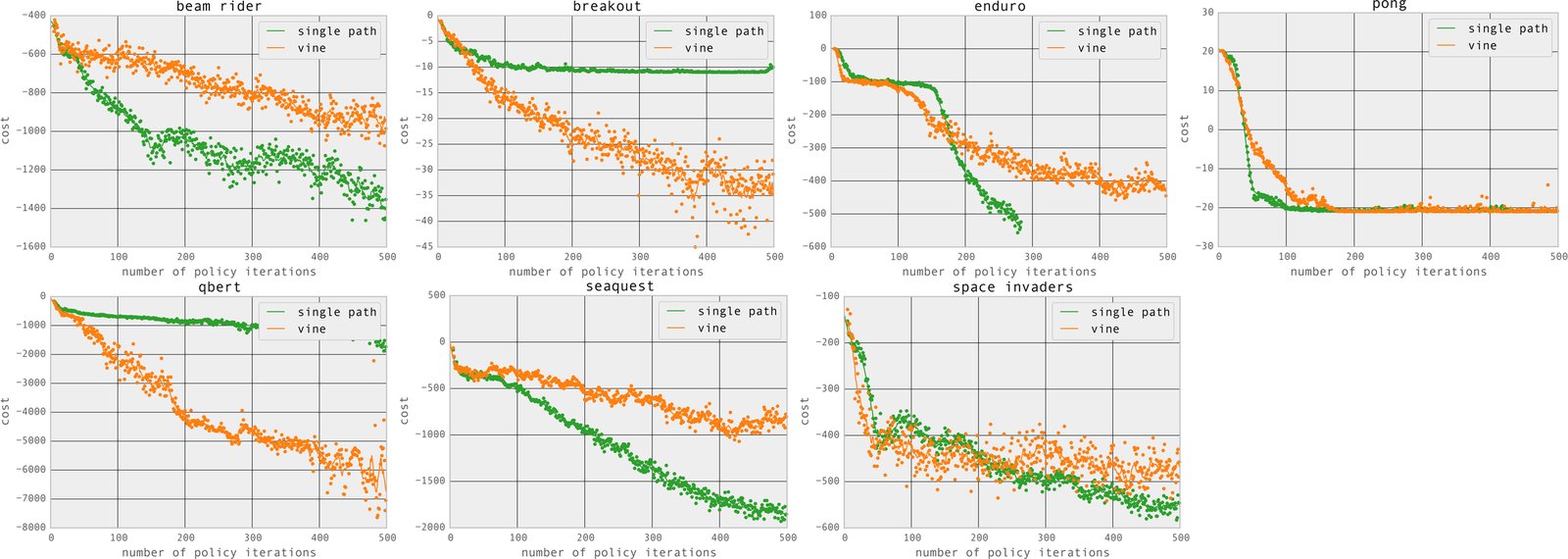
Figure 5: Learning curves for the Atari domain. For historical reasons, the plots show cost = negative reward.
图 5:Atari 域学习曲线。因历史原因,图中显示 cost = 负奖励。