Transporter Networks: Rearranging the Visual World for Robotic Manipulation

Transporter Networks：为机器人操作重排视觉世界

Andy Zeng    Pete Florence    Jonathan Tompson    Stefan Welker    Jonathan Chien Affiliation:  Maria Attarian, Travis Armstrong, Ivan Krasin, Dan Duong Affiliation:  Ayzaan Wahid, Vikas Sindhwani, Johnny Lee Affiliation:  Robotics at Google

Abstract

摘要

Robotic manipulation can be formulated as inducing a sequence of spatial displacements: where the space being moved can encompass an object, part of an object, or end effector. In this work, we propose the Transporter Network, a simple model architecture that rearranges deep features to infer spatial displacements from visual input – which can parameterize robot actions. It makes no assumptions of objectness (e.g. canonical poses, models, or keypoints), it exploits spatial symmetries, and is orders of magnitude more sample efficient than our benchmarked alternatives in learning vision-based manipulation tasks: from stacking a pyramid of blocks, to assembling kits with unseen objects; from manipulating deformable ropes, to pushing piles of small objects with closed-loop feedback. Our method can represent complex multi-modal policy distributions and generalizes to multi-step sequential tasks, as well as 6DoF pick-and-place. Experiments on 10 simulated tasks show that it learns faster and generalizes better than a variety of end-to-end baselines, including policies that use ground-truth object poses. We validate our methods with hardware in the real world. Experiment videos and code will be made available at https://transporternets.github.io

机器人操作可以表述为诱导一串空间位移：被移动的空间可以是物体、物体局部或末端执行器。本文提出 Transporter Network，一种简洁的模型结构，通过对深度特征做重排，从视觉输入推断空间位移，并据此参数化机器人动作。它不做物体性假设（例如规范位姿、模型或关键点），利用空间对称性，在学习基于视觉的操作任务上，样本效率比我们对照的基线高出数个数量级：从堆叠积木金字塔，到用未见过的物体组装套件；从操作可变形绳索，到用闭环反馈推动小物体堆。该方法能表示复杂的多峰策略分布，可泛化到多步序列任务以及六自由度抓取放置。在 10 项仿真任务上的实验表明，它比多种端到端基线学得更快、泛化更好，其中包括使用真实物体位姿的策略。我们在真实硬件上验证了方法。实验视频与代码见 https://transporternets.github.io

Keywords: Deep Learning, Vision, Manipulation

关键词： 深度学习、视觉、操作

1 Introduction

1 引言

End-to-end models that map directly from pixels to actions hold the capacity to learn complex manipulation skills, but are known to require copious amounts of data [1, 2]. Integrating object-centric assumptions – e.g., object keypoints [3, 4, 5, 6], embeddings [7, 8], or dense descriptors [9, 10, 11] – has been shown to improve sample efficiency [10]. However, these representations often impose data collection burdens (i.e., configuring scenes with specific singulated objects) and still struggle to address challenging scenarios with unseen classes of objects, occluded objects, highly deformable objects, or piles of small objects [12]. This naturally leads us to ask: is there structure that we can incorporate into our end-to-end models to improve their learning efficiency, without imposing any of the limitations or burdens of explicit object representations?

直接从像素映射到动作的端到端模型具备学习复杂操作技能的能力，但已知需要大量数据 [1, 2]。融入以物体为中心的假设——例如物体关键点 [3, 4, 5, 6]、嵌入 [7, 8] 或稠密描述子 [9, 10, 11]——已被证明能提升样本效率 [10]。然而这些表示往往加重数据采集负担（例如必须布置可分离的特定物体场景），在未见物体类别、遮挡物体、高度可变形物体或小物体堆等场景上仍然吃力 [12]。这自然引出一个问题：能否在端到端模型中引入结构以提高学习效率，同时又不施加显式物体表示带来的限制或负担？

In this work, we propose the Transporter Network, a simple end-to-end model architecture that preserves spatial structure for vision-based manipulation, without object-centric assumptions:

本文提出 Transporter Network，一种简洁的端到端模型结构，在基于视觉的操作中保留空间结构，且不做以物体为中心的假设：

• • Manipulation involves rearranging things, which can be thought of as executing a sequence of spatial displacements: where the space being moved (i.e., transported) can encompass an object(s), part of an object, or end effector. We formulate vision for manipulation as estimating these displacements. Transporter Networks directly optimize for this by learning to 1) attend to a local region, and 2) predict its target spatial displacement via deep feature template matching – which then parameterizes robot actions for manipulation. This formulation enables high-level perceptual reasoning about which visual cues are important, and how they should be rearranged in a scene – the distributions of which can be learned from demonstrations.

• • 操作涉及重排事物，可视为执行一串空间位移：被移动（即被搬运）的空间可以涵盖物体、物体局部或末端执行器。我们将面向操作的视觉问题表述为估计这些位移。Transporter Networks 通过学习 1）关注局部区域，以及 2）借助深度特征模板匹配预测其目标空间位移，直接为此优化——随后用该位移参数化操作动作。这一表述支持关于哪些视觉线索重要、它们应如何在场景中重排的高层感知推理——其分布可从示范中学习。

• • Transporter Networks preserve the 3D spatial structure of the visual input. Prior end-to-end models [1, 2] often use convolutional architectures with raw images, in which valuable spatial information can be lost to perspective distortions. Our method uses 3D reconstruction to project visual data onto a spatially-consistent representation as input, with which it is able to better exploit equivariance [13, 14] for inductive biases that are present within the geometric symmetries [15] of the data for more efficient learning.

• • Transporter Networks 保留视觉输入的三维空间结构。先前端到端模型 [1, 2] 常对原始图像使用卷积结构，宝贵的空间信息可能因透视畸变而丢失。我们的方法用三维重建把视觉数据投影到空间一致的表示作为输入，从而更好地利用数据几何对称性 [15] 中已有的等变性 [13, 14] 作为归纳偏置，实现更高效的学习。

In our experiments, Transporter Networks exhibit superior sample efficiency on a number of tabletop manipulation tasks that involve changing the state of the robot’s environment in a purposeful manner: from stacking a pyramid of blocks, to assembling kits with unseen objects; from manipulating deformable ropes, to pushing piles of small objects with closed-loop feedback. Transporter Networks excel in modeling multi-modal spatial action distributions, and by construction generalize across rotations and translations of objects. They do not require any prior knowledge of the objects to be manipulated – they rely only on information contained within partial RGB-D data from demonstrations, and are capable of generalizing to new objects and configurations, and for some tasks, one-shot learning from a single demonstration.

实验中，Transporter Networks 在多项桌面操作任务上表现出更优的样本效率，这些任务都以有目的地改变机器人环境状态为目标：从堆叠积木金字塔，到用未见物体组装套件；从操作可变形绳索，到用闭环反馈推动小物体堆。Transporter Networks 擅长建模多峰空间动作分布，并在构造上对物体的旋转与平移泛化。它们不需要关于待操作物体的先验知识——只依赖示范中部分 RGB-D 数据所含信息，并能泛化到新物体与新构型；对部分任务，还能从单次示范做一次性学习。

Our main contribution is a new perspective on the role of spatial structure and its capacity to improve end-to-end learning for vision-based manipulation. We propose a simple model architecture that learns to attend to a local region and predict its spatial displacement, while retaining the spatial structure of the visual input. On 10 unique tabletop manipulation tasks, Transporter Networks trained from scratch are capable of achieving greater than 90% success on most tasks with objects in new configurations using 100 expert demonstrations, while other end-to-end alternatives struggle to generalize with the same amount of data. We also develop an extension to 6DoF tasks by combining 3DoF Transporter Networks with continuous regression to handle the remaining degrees of freedom. To facilitate further research in vision-based manipulation, we plan release code and open-source Ravens, our new simulated benchmark with all tasks. Ravens features a Gym-like API [16] with a built-in stochastic oracle to evaluate the sample efficiency of imitation learning methods.

我们的主要贡献是重新审视空间结构在提升基于视觉操作的端到端学习中的作用。我们提出一种简洁模型：学习关注局部区域并预测其空间位移，同时保留视觉输入的空间结构。在 10 项独特的桌面操作任务上，从零训练的 Transporter Networks 在多数任务上，用 100 条专家示范即可在物体新构型下达到超过 90% 的成功率，而其他端到端方案在同等数据量下难以泛化。我们还通过将三维自由度 Transporter Networks 与连续回归结合，扩展到六自由度任务。为促进基于视觉操作的进一步研究，我们计划开源代码并开源 Ravens——包含全部任务的新仿真基准。Ravens 提供类 Gym 的 API [16]，内置随机 oracle，用于评估模仿学习方法的样本效率。

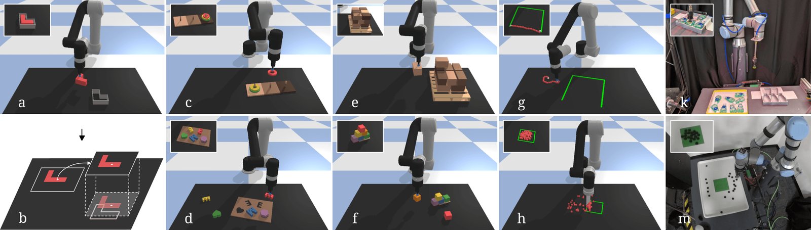
Figure 1: A Transporter Network is a simple model architecture that attends to a local region and predicts its spatial displacement (b) from visual input – which can parameterize robot actions. It is sample efficient in learning complex vision-based manipulation tasks: inserting blocks into fixtures (a), sequential pick-and-place in Towers of Hanoi (c), assembling kits with unseen objects (d), palletizing boxes (e), stacking a pyramid of blocks (f), manipulating rope (g), and pushing piles of small objects with closed-loop feedback (h) – and is practical to deploy on real production robots (k, m).

图 1：Transporter Network 是一种简洁的模型结构，从视觉输入关注局部区域并预测其空间位移（b）——可据此参数化机器人动作。它在学习复杂的基于视觉的操作任务上样本效率高：把积木插入夹具（a）、河内塔中的序列抓取放置（c）、用未见物体组装套件（d）、码垛纸箱（e）、堆叠积木金字塔（f）、操作绳索（g），以及用闭环反馈推动小物体堆（h）——并适合部署在真实产线机器人上（k, m）。

2 Related Work

2 相关工作

Object-centric Representations. Considerable research in vision for manipulation has been devoted to object detectors and pose estimators [17, 18, 19, 20, 21]. These methods often require object-specific training data, making them difficult to scale to applications with unseen objects. Alternative representations including keypoints [3, 4, 5, 6] and dense descriptors [9, 10, 11] have shown to be capable of category-level generalization and representing deformable objects, but still struggle to represent scenes with an unknown number of objects (e.g., piles of small objects) or occluded objects. End-to-end models for vision-based manipulation learn faster when integrated with such object-centric representations [10], providing sample-efficiency benefits but retaining the data-collection and representational constraints of object-centricness. In this work, we show that it is possible to achieve sample efficient end-to-end learning without object-centric representations – enabling the same model architecture to generalize to tasks with unseen objects, variable numbers of objects, deformable objects, and piles of small objects.

以物体为中心的表示。 面向操作的视觉研究大量投入物体检测与位姿估计 [17, 18, 19, 20, 21]。这些方法常需要物体特定训练数据，难以扩展到未见物体的应用。替代表示包括关键点 [3, 4, 5, 6] 与稠密描述子 [9, 10, 11]，已能做类别级泛化并表示可变形物体，但在物体数量未知（例如小物体堆）或存在遮挡时仍吃力。集成这类以物体为中心表示时，基于视觉操作的端到端模型学得更快 [10]，带来样本效率收益，却仍保留以物体为中心的数据采集与表示约束。本文表明，无需以物体为中心的表示也能实现样本高效的端到端学习——从而使同一模型结构泛化到未见物体、可变物体数量、可变形物体以及小物体堆等任务。

Pick-and-Place has had a long history in robotics, motivated by industrial needs. Classic systems use pose estimation of known objects [17, 18], as well as scripted planning and motion control [22]. While robust in structured settings (e.g., manufacturing), these systems are difficult to deploy in unstructured settings (e.g., logistics, agriculture, household) – leading to renewed interest in leveraging learned models to achieve general pick-and-place policies [23, 24, 25, 26, 27, 28, 29, 30] that can handle unseen objects. We benchmark against the more recent Form2Fit [24] on multiple tasks, and demonstrate that Transporter Networks are better able to handle tasks that require precise placing, multi-step sequencing, and closed-loop visual feedback.

抓取与放置 在机器人学中历史悠久，受工业需求驱动。经典系统对已知物体做位姿估计 [17, 18]，并配合脚本化规划与运动控制 [22]。在结构化场景（如制造）中稳健，但在非结构化场景（如物流、农业、家居）难部署——于是人们重新关注用学习模型获得能处理未见物体的通用抓取放置策略 [23, 24, 25, 26, 27, 28, 29, 30]。我们在多项任务上与较新的 Form2Fit [24] 对照，表明 Transporter Networks 更能处理需要精确放置、多步排序与闭环视觉反馈的任务。

3 Method

3 方法

Consider the problem of learning pick-and-place actions $\mathbf{a}_{t}$ with a robot from visual observations $\mathbf{o}_{t}$:

考虑从视觉观测 $\mathbf{o}_{t}$ 学习抓取放置动作 $\mathbf{a}_{t}$ 的问题：

$$f(\mathbf{o}_{t})\rightarrow\mathbf{a}_{t}=(\mathcal{T}_{\textrm{pick}},\mathcal{T}_{\textrm{place}})\in\mathcal{A}$$

where $\mathcal{T}_{\textrm{pick}}$ is the pose of the end effector used to pick an object, and $\mathcal{T}_{\textrm{place}}$ to place the object. Both poses can be defined in SE(2) or SE(3), depending on the task and degrees of freedom available to the end effector. We can generalize beyond pick-and-place by considering manipulation with other motion primitives [22] that are also parameterized by two end effector poses. For example, we can parameterize pushing, where $\mathcal{T}_{\textrm{pick}}$ is instead the pose of the end effector at the start of the push, and $\mathcal{T}_{\textrm{place}}$ is where it moves to complete the push. In this work, we consider tasks that can be completed by a sequence of two-pose motion primitives. In the following section, we begin by describing our approach in the context of planar pick-and-place. We then discuss extensions to 6DoF pick-and-place, sequential multi-step tasks, and motion-primitive-based manipulation of deformable objects and piles of objects.

其中 $\mathcal{T}_{\textrm{pick}}$ 是用于抓取物体的末端执行器位姿，$\mathcal{T}_{\textrm{place}}$ 用于放置。二者可定义在 SE(2) 或 SE(3) 上，取决于任务与末端可用自由度。我们还可把问题推广到由两个末端位姿参数化的其他运动基元 [22] 的操作。例如可参数化推动：此时 $\mathcal{T}_{\textrm{pick}}$ 是推动开始时末端位姿，$\mathcal{T}_{\textrm{place}}$ 是完成推动时末端到达的位姿。本文考虑可由一串双位姿运动基元完成的任务。下一节先在平面抓取放置语境下描述方法，再讨论扩展到六自由度抓取放置、序列多步任务，以及基于运动基元的可变形物体与物体堆操作。

3.1 Learning to Transport

3.1 学习搬运

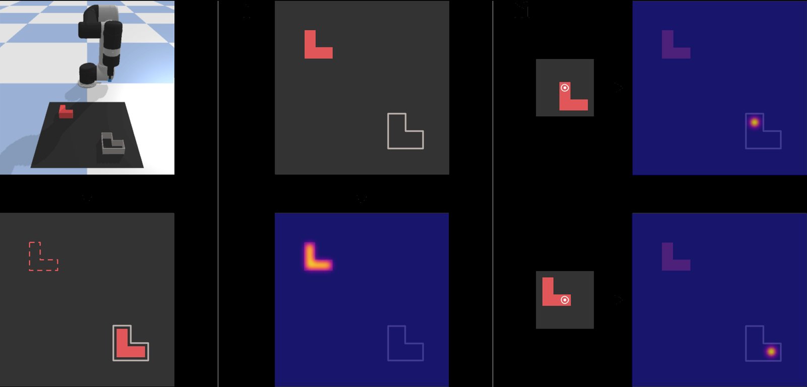
Figure 2: Simple planar pick-and-place task where (i) there is a distribution of successful pick poses, and (ii) for each successful pick pose, there is a corresponding distribution of successful place poses.

图 2：简单的平面抓取放置任务：(i) 存在成功抓取位姿的分布；(ii) 对每个成功抓取位姿，存在对应的成功放置位姿分布。

Consider the planar pick-and-place problem on the right, where $\mathcal{T}_{\textrm{pick}},\mathcal{T}_{\textrm{place}}\in\mathbb{R}^{2}$ are 2D coordinates. In this task, the goal is to pick up the red block with an immobilizing grasp (e.g., with a suction gripper), then place it into the fixture. This simple setting reveals two fundamental aspects of the pick-and-place problem: (i) there may be a distribution of successful pick poses (from which $\mathcal{T}_{\textrm{pick}}$ may be sampled e.g., on the surface of the block), and (ii) for each successful pick pose, there is a corresponding distribution of successful place poses (from which $\mathcal{T}_{\textrm{place}}$ may be sampled).

考虑右侧的平面抓取放置问题，其中 $\mathcal{T}_{\textrm{pick}},\mathcal{T}_{\textrm{place}}\in\mathbb{R}^{2}$ 为二维坐标。任务目标是用固定抓取（例如吸盘）拿起红色积木，再放入夹具。这一简单设定揭示了抓取放置问题的两个基本方面：(i) 可能存在成功抓取位姿的分布（可从中采样 $\mathcal{T}_{\textrm{pick}}$，例如在积木表面上），以及 (ii) 对每个成功抓取位姿，存在对应的成功放置位姿分布（可从中采样 $\mathcal{T}_{\textrm{place}}$）。

The goal of Transporter Networks is to recover these distributions from visual observations alone – without assumptions of objectness. While assigning canonical poses to the block and fixture might simplify the problem, there are many benefits to avoiding such object-centric representations – including the capacity to handle unseen objects, deformable objects, and uncountable piles of small objects. Hence we assume no prior information about the objects (e.g., no 3D models, poses, class categories, keypoints, etc.).

Transporter Networks 的目标是仅从视觉观测恢复这些分布——不做物体性假设。给积木与夹具分配规范位姿或许能简化问题，但避免此类以物体为中心的表示有诸多好处——包括处理未见物体、可变形物体以及不可数的小物体堆的能力。因此我们假设对物体没有先验信息（例如没有三维模型、位姿、类别、关键点等）。

Transporter Networks decompose the problem into (i) picking and (ii) pick-conditioned placing:

Transporter Networks 把问题分解为 (i) 抓取与 (ii) 以抓取为条件的放置：

$$f_{\textrm{pick}}(\mathbf{o}_{t})\rightarrow\mathcal{T}_{\textrm{pick}}\qquad\qquad\qquad\qquad f_{\textrm{place}}(\mathbf{o}_{t},\mathcal{T}_{\textrm{pick}})\rightarrow\mathcal{T}_{\textrm{place}}$$

We present a solution to both with Transporter Networks – but in this work, our primary contribution is on (ii), pick-conditioned placing via transporting. We first begin by briefly describing (i), picking.

我们用 Transporter Networks 对二者都给出解——但本文主要贡献在 (ii)，即通过搬运实现以抓取为条件的放置。先简要描述 (i) 抓取。

Learning Picking. Our visual observation $\mathbf{o}_{t}$ is a projection of the scene (e.g., reconstructed from RGB-D images), defined on a regular grid of pixels $\{(u,v)\}$ at timestep $t$ of a sequential rearrangement task. Through camera-to-robot calibration, we can correspond each pixel in $\mathbf{o}_{t}$ to a picking action at that location: $\mathcal{T}_{\textrm{pick}}\sim(u,v)\in\mathbf{o}_{t}$. The distribution of successful picks over pixels in $\mathbf{o}_{t}$ can be multi-modal in nature – particularly in cases when there are multiple instances of the same object in the scene, or when there are symmetries in the shapes of objects. As in prior works [31, 32, 33], Transporter Networks use fully convolutional networks (FCNs, commonly used in vision for image segmentation tasks [34]) to model an action-value function $\mathcal{Q}_{\textrm{pick}}((u,v)|\mathbf{o}_{t})$ that correlates with picking success (architecture in Sec. 3.2):

学习抓取。 视觉观测 $\mathbf{o}_{t}$ 是场景的投影（例如由 RGB-D 图像重建），定义在规则像素网格 $\{(u,v)\}$ 上，对应序列重排任务的时刻 $t$。经相机—机器人标定，可将 $\mathbf{o}_{t}$ 中每个像素对应到该位置的抓取动作：$\mathcal{T}_{\textrm{pick}}\sim(u,v)\in\mathbf{o}_{t}$。$\mathbf{o}_{t}$ 上成功抓取在像素上的分布可以是多峰的——尤其当场景中有多个同类物体实例，或物体形状具有对称性时。与先前工作 [31, 32, 33] 一样，Transporter Networks 用全卷积网络（FCN，常用于图像分割等视觉任务 [34]）建模与抓取成功相关的动作价值函数 $\mathcal{Q}_{\textrm{pick}}((u,v)|\mathbf{o}_{t})$（结构见第 3.2 节）：

$$\mathcal{T}_{\textrm{pick}}=\argmax_{(u,v)}\ \mathcal{Q}_{\textrm{pick}}((u,v)|\mathbf{o}_{t})$$

FCNs are translationally equivariant by nature, which synergizes with spatial action representations: if an object to be picked in the scene is translated, then the picking pose also translates. Formally, equivariance here can be characterized as $f_{\textrm{pick}}(g\circ\mathbf{o}_{t})=g\circ f_{\textrm{pick}}(\mathbf{o}_{t})$, where $g$ is a translation. Spatial equivariance has previously been shown to improve learning efficiency for vision-based picking [29, 31, 32, 33, 35]. To this end, FCNs excel in modeling complex multi-modal picking distributions anchored on visual features.

FCN 天生具有平移等变性，与空间动作表示相得益彰：若场景中待抓取物体平移，抓取位姿也平移。形式上，这里的等变性可写作 $f_{\textrm{pick}}(g\circ\mathbf{o}_{t})=g\circ f_{\textrm{pick}}(\mathbf{o}_{t})$，其中 $g$ 是平移。先前工作已表明空间等变性可提升基于视觉抓取的学习效率 [29, 31, 32, 33, 35]。因此，FCN 擅长建模锚定在视觉特征上的复杂多峰抓取分布。

Spatially Consistent Visual Representations. The benefits of spatial equivariance are most pronounced when observations $\mathbf{o}_{t}$ are spatially consistent, meaning that the appearance of an object remains constant across different camera views, as well as across spatial transforms of rigid objects. This is in contrast to perspective images, in which the appearance of an object could scale or distort depending on the camera view and lens properties. In practice, spatial consistency also simplifies data augmentation during training, since applying rigid transforms to $\mathbf{o}_{t}$ can yield data that appears as if objects in the scene were physically reconfigured. As with perspective images, however, spatially consistent representations still retain challenges from partial visibility and occlusion. As in [33], we convert RGB-D images into a spatially consistent form by unprojecting to a 3D point cloud, then rendering into an orthographic projection, in which each pixel $(u,v)$ represents a fixed window of 3D space (Fig. 3a). Unlike in prior work, we use this spatially consistent representation for the transport operation, which we describe next.

空间一致的视觉表示。 当观测 $\mathbf{o}_{t}$ 空间一致时，空间等变性的收益最明显：物体外观在不同相机视角下保持恒定，刚性物体在空间变换下外观也保持恒定。这与透视图像不同——透视下物体外观可能随视角与镜头特性缩放或畸变。实践中，空间一致性也简化训练时的数据增强，因为对 $\mathbf{o}_{t}$ 施加刚性变换可得到看起来像场景中物体被物理重配的数据。不过与透视图像一样，空间一致表示仍保留部分可见与遮挡带来的挑战。与 [33] 一样，我们将 RGB-D 图像反投影为三维点云，再渲染成正交投影，使每个像素 $(u,v)$ 对应工作空间中固定窗口的三维空间（图 3a）。与先前工作不同，我们把这种空间一致表示用于接下来的搬运操作。

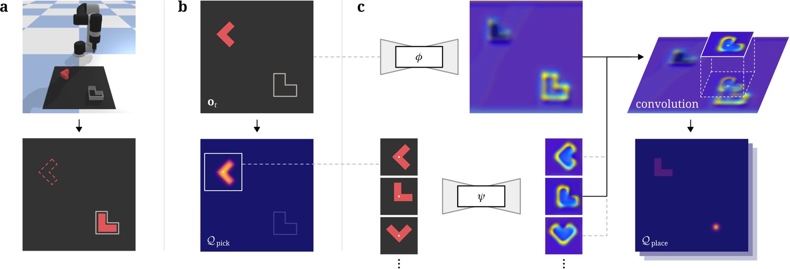
Figure 3: In this setting (a) where the task is to pick up the red block with an immobilizing grasp (e.g., suction) and place it into the fixture, the goal of Transporter Networks is to recover the distribution of successful picks (b), and distribution of successful placements (c) conditioned on a sampled pick. For pick-conditioned placing (c), deep feature template matching occurs with a local crop around the sampled pick as the exemplar. Rotations of the crop around the pick are used to decode the best placing rotation. Our method preserves rotation and translation equivariance for efficient learning.

图 3：在此设定 (a) 中，任务是用固定抓取（例如吸盘）拿起红色积木并放入夹具；Transporter Networks 的目标是恢复成功抓取分布 (b)，以及以采样抓取为条件的成功放置分布 (c)。对以抓取为条件的放置 (c)，以采样抓取周围的局部裁剪作为范例做深度特征模板匹配。围绕抓取旋转裁剪，用以解码最佳放置旋转。我们的方法保留旋转与平移等变性，以实现高效学习。

Learning Pick-Conditioned Placing via Transporting. Spatially consistent visual representations enable us to perform visuo-spatial transporting, in which dense pixel-wise features from a partial crop $\mathbf{o}_{t}[\mathcal{T}_{\textrm{pick}}]$ centered on $\mathcal{T}_{\textrm{pick}}$ are rigidly transformed then overlaid on top of another partial crop $\mathbf{o}_{t}[\tau]$ centered on a candidate place pose $\tau$, where $\mathbf{o}_{t}$ is the observation before the pick. Intuitively, if the crop encompasses an object, then this operation can be thought of as imagining the object at another location in the scene. Fig. 3c shows this in the context of overlaying the red block across the scene to find its placement in the fixture.

通过搬运学习以抓取为条件的放置。 空间一致的视觉表示使我们能做视觉—空间搬运：把以 $\mathcal{T}_{\textrm{pick}}$ 为中心的局部裁剪 $\mathbf{o}_{t}[\mathcal{T}_{\textrm{pick}}]$ 上的稠密像素特征刚性变换后，叠加到以候选放置位姿 $\tau$ 为中心的另一局部裁剪 $\mathbf{o}_{t}[\tau]$ 上，其中 $\mathbf{o}_{t}$ 是抓取前的观测。直观上，若裁剪涵盖一个物体，该操作可理解为想象该物体出现在场景另一位置。图 3c 展示了把红色积木在场景中叠加以寻找其在夹具中放置位置的情形。

In this work, the goal of Transporter Networks is to transport our partial crop $\mathbf{o}_{t}[\mathcal{T}_{\textrm{pick}}]$ densely across a set of poses $\{\tau_{i}\}$ to search for its best placement, i.e. the $\mathbf{o}_{t}[\tau_{i}]$ with the highest feature correlation. This operation is analogous to the search function in visual tracking literature [36, 37, 38] where $\mathbf{o}_{t}[\mathcal{T}_{\textrm{pick}}]$ is the exemplar and $\mathbf{o}_{t}$ is the search area, or in retrieval systems literature where $\mathbf{o}_{t}[\mathcal{T}_{\textrm{pick}}]$ is the query and $\mathbf{o}_{t}$ is the key. We formulate this as a template matching problem, using cross-correlation with dense feature embeddings $\psi(\cdot)$ and $\phi(\cdot)$ from two deep models:

在本文中，Transporter Networks 的目标是把局部裁剪 $\mathbf{o}_{t}[\mathcal{T}_{\textrm{pick}}]$ 稠密地搬运到一组位姿 $\{\tau_{i}\}$ 上，搜索其最佳放置，即特征相关最高的 $\mathbf{o}_{t}[\tau_{i}]$。该操作类似于视觉跟踪文献中的搜索函数 [36, 37, 38]——其中 $\mathbf{o}_{t}[\mathcal{T}_{\textrm{pick}}]$ 是范例、$\mathbf{o}_{t}$ 是搜索区域；或检索系统文献中 $\mathbf{o}_{t}[\mathcal{T}_{\textrm{pick}}]$ 是查询、$\mathbf{o}_{t}$ 是键。我们将其表述为模板匹配问题，用两个深度模型的稠密特征嵌入 $\psi(\cdot)$ 与 $\phi(\cdot)$ 做互相关：

$$\mathcal{Q}_{\textrm{place}}(\tau|\mathbf{o}_{t},\mathcal{T}_{\textrm{pick}})=\psi(\mathbf{o}_{t}[\mathcal{T}_{\textrm{pick}}])*\phi(\mathbf{o}_{t})[\tau],\qquad\mathcal{T}_{\textrm{place}}=\argmax_{\{\tau_{i}\}}\ \mathcal{Q}_{\textrm{place}}(\tau_{i}|\mathbf{o}_{t},\mathcal{T}_{\textrm{pick}}) \tag{1}$$

where $\mathcal{Q}_{\textrm{place}}(\tau|\mathbf{o}_{t},\mathcal{T}_{\textrm{pick}})$ is an action-value function that correlates with placing success, and $\tau$ covers the space of all possible placing poses – which is equivalent to the space of 2D translations across $\mathbf{o}_{t}$ in our first simple red block and fixture example. Since $\mathbf{o}_{t}$ is spatially consistent, the structure of dense features $\psi(\mathbf{o}_{t})$ and $\phi(\mathbf{o}_{t})$ are also spatially consistent. A key property is that Eq. 1 is invariant to $\mathcal{T}_{\textrm{pick}}$ as long as cross-correlation via transform $\mathcal{T}_{\textrm{place}}$ produces the desired imagined overlay. This enables learning pick-conditioned placing from few examples (Fig. 5), without having to train over all possible picks [27]. Note that it is the deep features, not the RGB-D pixels, which are overlaid, and that the influence of the overlay extends beyond the crop, since for each dense pixel in feature space, the receptive field is large.

其中 $\mathcal{Q}_{\textrm{place}}(\tau|\mathbf{o}_{t},\mathcal{T}_{\textrm{pick}})$ 是与放置成功相关的动作价值函数，$\tau$ 覆盖所有可能放置位姿的空间——在我们第一个简单红积木与夹具例子中，等价于 $\mathbf{o}_{t}$ 上的二维平移空间。由于 $\mathbf{o}_{t}$ 空间一致，稠密特征 $\psi(\mathbf{o}_{t})$ 与 $\phi(\mathbf{o}_{t})$ 的结构也空间一致。一个关键性质是：只要经由变换 $\mathcal{T}_{\textrm{place}}$ 的互相关能产生期望的想象叠加，式 1 对 $\mathcal{T}_{\textrm{pick}}$ 不变。这使得能从少量例子学习以抓取为条件的放置（图 5），而无需对所有可能抓取训练 [27]。注意被叠加的是深度特征而非 RGB-D 像素，且叠加的影响超出裁剪范围，因为特征空间中每个稠密像素的感受野都很大。

Learning with Planar Rotations in SE(2). Our first example uses only pick-and-place actions in the space of 2D translations – however, $\mathcal{T}_{\textrm{pick}}$ and $\mathcal{T}_{\textrm{place}}$ may also represent rotations as in Fig. 3. In the planar SE(2) case, we discretize the space of SO(2) rotations into $k$ bins, then rotate the input visual observation $\mathbf{o}_{t}$ for each bin. $\mathbf{o}_{t}$ is thereby defined on a grid of voxels $\{(u,v,w)_{i}\}$ where $w$ lies on the $k$-discretized axis of rotations, and $\mathcal{T}_{\textrm{pick}}$ and $\mathcal{T}_{\textrm{place}}$ are represented discretely on this grid in SE(2). In practice, this is achieved by running the FCN $k$ times in parallel, once for each rotated $\mathbf{o}_{t}$, sharing model weights across all rotations.

在 SE(2) 中学习平面旋转。 第一个例子只用二维平移空间中的抓取放置动作——但如图 3，$\mathcal{T}_{\textrm{pick}}$ 与 $\mathcal{T}_{\textrm{place}}$ 也可表示旋转。在平面 SE(2) 情形下，我们将 SO(2) 旋转空间离散为 $k$ 个箱，并对每个箱旋转输入视觉观测 $\mathbf{o}_{t}$。于是 $\mathbf{o}_{t}$ 定义在体素网格 $\{(u,v,w)_{i}\}$ 上，其中 $w$ 位于 $k$ 离散的旋转轴上，$\mathcal{T}_{\textrm{pick}}$ 与 $\mathcal{T}_{\textrm{place}}$ 在该 SE(2) 网格上离散表示。实践中，通过对每个旋转后的 $\mathbf{o}_{t}$ 并行运行 FCN $k$ 次、并在所有旋转间共享模型权重来实现。

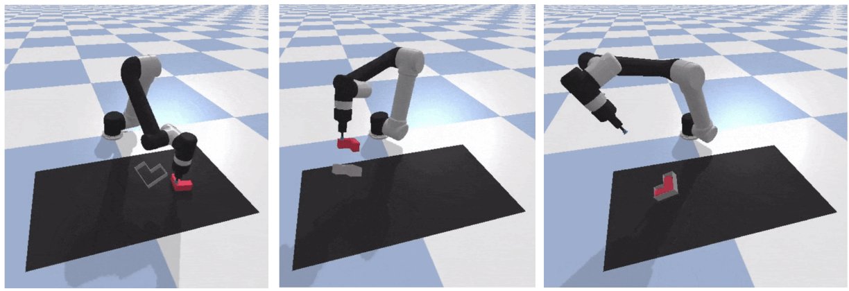
Figure 4: In this 6-DoF variant of the task presented in Fig. 3, the fixture location varies as well in the out-of-plane rotations ($r_{x}$, $r_{y}$), and height ($z$). Transporter Networks can address this task through multi-stage inference.

图 4：在图 3 任务的六自由度变体中，夹具位置在平面外旋转（$r_{x}$、$r_{y}$）与高度（$z$）上也变化。Transporter Networks 可通过多阶段推断应对该任务。

Learning with Full Rigid Body Transformations in SE(3). While the previous sections discussed learning a $\mathcal{Q}$ function over a discretized space, extending to the full SE(3) case to handle all six degrees of freedom of rigid objects becomes infeasible to sufficiently discretize the 6-dimensional space – due to the curse of dimensionality. However, interestingly we find the transport operation to be an enabling building block into higher dimensions, using a multi-stage approach to extend into tasks which require SE(3) placing. First, the three SE(2) degrees-of-freedom are addressed as in the previous section, producing an estimated $\hat{\mathcal{T}}^{\text{SE(2)}}_{\textrm{place}}$. Then, we extend the cross-correlation transport operation – rather than using one channel over SE(2) to classify the correct discretized action, we use three channels over SE(2) to regress the remaining rotational ($r_{x},r_{y}$) and translational ($z$-height) degrees of freedom. We use a $\psi^{\prime}$ and $\phi^{\prime}$ which are identical to the $\psi$ and $\phi$ used for SE(2) classification, but with three separate cross-correlations ($*_{3}$) from subsets of channels, and also add learnable nonlinearity after the cross-correlation via a three-headed MLP network, $f(\cdot)$: $r_{x},\ r_{y},\ z=f\big(\psi^{\prime}(\mathbf{o}_{t}[\mathcal{T}_{\textrm{pick}}])*_{3}\phi^{\prime}(\mathbf{o}_{t})[\hat{\mathcal{T}}^{\text{SE(2)}}_{\textrm{place}}]\big)$. This hybrid discrete/continuous approach affords a number of nice properties: the discrete SE(2) step is good at representing complex multi-modal distributions in those degrees of freedom, and once an approximate SE(2) alignment has been overlaid via the transport operation, this acts as an attention mechanism to aid the model in precise continuous regression. To handle multi-modality in the continuous degrees of freedom, we can regress mixture densities. In practice we have found that multiple approaches can work well once approximate SE(2) alignment has been applied, see the Appendix for more. Multi-stage SE(3) classification, using Eq. 1 iteratively, is also possible.

在 SE(3) 中学习完整刚体变换。 前几节讨论在离散空间上学习 $\mathcal{Q}$ 函数；扩展到完整 SE(3) 以处理刚体全部六个自由度时，充分离散六维空间因维度灾难而不可行。但有趣的是，我们发现搬运操作可作为进入更高维的积木块，用多阶段方法扩展到需要 SE(3) 放置的任务。首先，按上一节处理三个 SE(2) 自由度，得到估计 $\hat{\mathcal{T}}^{\text{SE(2)}}_{\textrm{place}}$。然后扩展互相关搬运操作——不再用 SE(2) 上的单通道对正确离散动作分类，而用 SE(2) 上的三通道回归剩余旋转（$r_{x},r_{y}$）与平移（$z$ 高度）自由度。我们使用与 SE(2) 分类中 $\psi$、$\phi$ 相同的 $\psi^{\prime}$、$\phi^{\prime}$，但从通道子集做三次独立互相关（$*_{3}$），并在互相关后经三头 MLP 网络 $f(\cdot)$ 加入可学习非线性：$r_{x},\ r_{y},\ z=f\big(\psi^{\prime}(\mathbf{o}_{t}[\mathcal{T}_{\textrm{pick}}])*_{3}\phi^{\prime}(\mathbf{o}_{t})[\hat{\mathcal{T}}^{\text{SE(2)}}_{\textrm{place}}]\big)$。这种离散/连续混合方法有若干优点：离散 SE(2) 步骤擅长表示这些自由度上的复杂多峰分布；一旦经搬运操作叠加近似 SE(2) 对齐，它又作为注意力机制，帮助模型做精确连续回归。对连续自由度上的多峰性，可回归混合密度。实践中我们发现，一旦施加近似 SE(2) 对齐，多种做法都能表现良好，详见附录。用式 1 迭代做多阶段 SE(3) 分类也是可行的。

Learning Sequential Pick-and-Place. Consider the challenging example with 3-disk Towers of Hanoi in Fig. 1c, where the task is to sequentially move 3 disks from the first tower to the third without placing a larger disk over a smaller disk. Completing this task requires correctly sequencing 7 pick-and-place actions. In this setup with a unique coloring of the base and disks, the task is Markovian. Hence actions can be directly conditioned on visual contextual cues, e.g., the next pick-and-place depends on the position (or absence due to occlusion) of observed objects in the scene. Our method is stateless, but experiments show that it can learn such sequencing behaviors through visual feedback. To enable this, it is important to increase the receptive field [39] of the FCNs to encompass most of the visual observation $\mathbf{o}_{t}$. Extending Transporter Networks with memory to handle non-Markovian tasks would be interesting future work.

学习序列抓取放置。 考虑图 1c 中三盘河内塔的挑战例子：任务是依次把三盘从第一塔移到第三塔，且不能把大盘放在小盘上。完成该任务需要正确排序 7 次抓取放置。在底座与圆盘着色唯一的设定下，任务是马尔可夫的。因此动作可直接以视觉上下文线索为条件，例如下一步抓取放置取决于场景中观测物体的位置（或因遮挡而缺失）。我们的方法是无状态的，但实验表明它能通过视觉反馈学习此类排序行为。为此，重要的是增大 FCN 的感受野 [39]，使其覆盖大部分视觉观测 $\mathbf{o}_{t}$。为 Transporter Networks 增加记忆以处理非马尔可夫任务，将是有趣的未来工作。

Manipulation Beyond Pick-and-Place: Deformables and Piles of Objects. Beyond pick-and-place of rigid objects, Transporter Networks can generalize to tasks that can be completed with two-pose primitives. For example, they can learn to sequentially rearrange a deformable rope such that it connects the two end points of an incomplete 3-sided square (Fig. 1e), or sequentially push piles of small objects into a desired target set (Fig. 1h) using a spatula-shaped end effector. In both cases, our experiments (Sec. 4) demonstrate that they can learn closed-loop behaviors using visual feedback to complete these tasks. Both tasks are characterized by dynamics that cannot be modeled with rigid displacements – however, our results suggest that rigid displacements can serve as a useful prior for non-rigid ones [40].

超越抓取放置的操作：可变形体与物体堆。 除刚性物体的抓取放置外，Transporter Networks 可泛化到可用双位姿基元完成的任务。例如，它们能学习依次重排可变形绳索，使其连接不完整三边正方形的两端点（图 1e）；或用铲形末端依次把小物体堆推入目标集合（图 1h）。两种情形下，实验（第 4 节）表明它们能用视觉反馈学习闭环行为以完成任务。两类任务的动力学都不能用刚性位移建模——但结果表明刚性位移可作为非刚性位移的有用先验 [40]。

3.2 Network Architecture

3.2 网络结构

Observation Space: For tabletop manipulation, our visual observation $\mathbf{o}_{t}$ is an orthographic top-down view of a $0.5{\times}1$m tabletop workspace, generated in simulation by fusing $480{\times}640$ RGB-D images captured with calibrated cameras using known intrinsics and extrinsics. The top-down image $\mathbf{o}_{t}$ has a pixel resolution of $160{\times}320$ – each pixel represents a $3.125{\times}3.125$mm vertical column of 3D space in the workspace. The image $\mathbf{o}_{t}$ contains both color (RGB) and scalar height-from-bottom (H) information, which enables the deep models to learn features that are rich in both visual texture and geometric shape.

观测空间： 对桌面操作，视觉观测 $\mathbf{o}_{t}$ 是 $0.5{\times}1$ m 桌面工作空间的正交俯视图，在仿真中由标定相机用已知内外参融合 $480{\times}640$ RGB-D 图像生成。俯视图 $\mathbf{o}_{t}$ 像素分辨率为 $160{\times}320$——每个像素表示工作空间中 $3.125{\times}3.125$ mm 的竖直三维柱。图像 $\mathbf{o}_{t}$ 同时含颜色（RGB）与自底部起的标量高度（H）信息，使深度模型能学习兼具视觉纹理与几何形状的丰富特征。

Picking: Our picking model is a single feed-forward FCN that takes as input the visual observation $\mathbf{o}_{t}\in\mathbb{R}^{H{\times}W{\times}4}$ and outputs dense pixel-wise values that correlate with picking success: $\mathcal{V}_{\textrm{pick}}\in\mathbb{R}^{H{\times}W}=\textrm{softmax}(\mathcal{Q}_{\textrm{pick}}((u,v)|\mathbf{o}_{t}))$. Our picking model is an hourglass encoder decoder architecture: a 43-layer residual network (ResNet) [41] with 12 residual blocks and 8-stride (3 2-stride convolutions in the encoder and 3 bilinear-upsampling layers in the decoder), followed by image-wide softmax. Each convolutional layer after the first is equipped with dilation [42], and interleaved with ReLU activations [43] before the last layer. 8-stride was chosen to balance between maximizing receptive field coverage per pixel prediction, while minimizing loss of resolution in the latent mid-level features of the network.

抓取： 抓取模型是单个前馈 FCN，输入视觉观测 $\mathbf{o}_{t}\in\mathbb{R}^{H{\times}W{\times}4}$，输出与抓取成功相关的稠密逐像素值：$\mathcal{V}_{\textrm{pick}}\in\mathbb{R}^{H{\times}W}=\textrm{softmax}(\mathcal{Q}_{\textrm{pick}}((u,v)|\mathbf{o}_{t}))$。抓取模型为沙漏编解码结构：43 层残差网络（ResNet）[41]，含 12 个残差块与 8 倍步幅（编码器中 3 个 2 倍步幅卷积，解码器中 3 个双线性上采样层），后接全图 softmax。第一层之后每个卷积层配备膨胀 [42]，并在最后一层前与 ReLU 激活 [43] 交错。选择 8 倍步幅是为了在最大化每个像素预测的感受野覆盖与最小化网络潜在中层特征分辨率损失之间取得平衡。

Placing: Our placing model is a two-stream feed-forward FCN that takes as input the visual observation $\mathbf{o}_{t}\in\mathbb{R}^{H{\times}W{\times}4}$ and outputs two dense feature maps: query features $\psi(\mathbf{o}_{t})\in\mathbb{R}^{H{\times}W{\times}d}$ and key features $\phi(\mathbf{o}_{t})\in\mathbb{R}^{H{\times}W{\times}d}$, where $d$ is the feature dimensionality. Our placing model shares a similar hourglass encoder decoder architecture as the picking model: each stream is an 8-stride 43-layer ResNet, but without non-linear activations in the last layer. A partial crop $\psi(\mathbf{o}_{t}[\mathcal{T}_{\textrm{pick}}])\in\mathbb{R}^{c{\times}c{\times}d}$ of query features with size $c$ centered around $\mathcal{T}_{\textrm{pick}}=\argmax{\mathcal{V}_{\textrm{pick}}}$ is transformed by $\tau$ (which covers the space of possible placement configurations), then cross-correlated (Eq. 1) with the key feature map $\phi(\mathbf{o}_{t})$ to output dense pixel-wise values that correlate with placing success: $\mathcal{V}_{\textrm{place}}\in\mathbb{R}^{H{\times}W{\times}k}=\textrm{softmax}(\mathcal{Q}_{\textrm{place}}(\tau|\mathbf{o}_{t},\mathcal{T}_{\textrm{pick}}))$ where $\tau$ is discretized into $k=36$ angles (multiples of 10*∘). The translation and rotation $\tau$ which gives the highest correlation with the partial crop, via $\psi(\mathbf{o}{t}[\mathcal{T}{\textrm{pick}}])\phi(\mathbf{o}{t})[\tau],$gives$\mathcal{T}{\textrm{place}}=\argmax{\mathcal{V}_{\textrm{place}}}$. Note that this operation can be made fast if implemented with highly optimized matrix multiplication (where the crop is flattened) or as a convolution (where the crop is the convolving kernel). Total inference time (with both picking and placing models) amounts to 200ms on an Nvidia GTX 2080 GPU.

放置： 放置模型是双流前馈 FCN，输入视觉观测 $\mathbf{o}_{t}\in\mathbb{R}^{H{\times}W{\times}4}$，输出两张稠密特征图：查询特征 $\psi(\mathbf{o}_{t})\in\mathbb{R}^{H{\times}W{\times}d}$ 与键特征 $\phi(\mathbf{o}_{t})\in\mathbb{R}^{H{\times}W{\times}d}$，其中 $d$ 为特征维数。放置模型与抓取模型共享类似的沙漏编解码结构：每流为 8 倍步幅的 43 层 ResNet，但最后一层无非线性激活。以 $\mathcal{T}_{\textrm{pick}}=\argmax{\mathcal{V}_{\textrm{pick}}}$ 为中心、尺寸为 $c$ 的查询特征局部裁剪 $\psi(\mathbf{o}_{t}[\mathcal{T}_{\textrm{pick}}])\in\mathbb{R}^{c{\times}c{\times}d}$，经 $\tau$（覆盖可能放置构型空间）变换后，与键特征图 $\phi(\mathbf{o}_{t})$ 做互相关（式 1），输出与放置成功相关的稠密逐像素值：$\mathcal{V}_{\textrm{place}}\in\mathbb{R}^{H{\times}W{\times}k}=\textrm{softmax}(\mathcal{Q}_{\textrm{place}}(\tau|\mathbf{o}_{t},\mathcal{T}_{\textrm{pick}}))$，其中 $\tau$ 离散为 $k=36$ 个角度（$10^{\circ}$ 的倍数）。与局部裁剪相关最高的平移与旋转 $\tau$，即经 $\psi(\mathbf{o}_{t}[\mathcal{T}_{\textrm{pick}}])*\phi(\mathbf{o}_{t})[\tau]$ 得到 $\mathcal{T}_{\textrm{place}}=\argmax{\mathcal{V}_{\textrm{place}}}$。注意若用高度优化的矩阵乘法（裁剪展平）或卷积（裁剪作为卷积核）实现，该操作可很快。抓取与放置模型合计推理时间在 Nvidia GTX 2080 GPU 上约 200 ms。

3.3 Training: Learning from Demonstrations

3.3 训练：从示范中学习

We assume access to a dataset $\mathcal{D}=\{\zeta_{1},\zeta_{2},...,\zeta_{n}\}$ of $n$ expert demonstrations, where each trajectory $\zeta_{i}=\{(\mathbf{o}_{0},\mathbf{a}_{0}),(\mathbf{o}_{1},\mathbf{a}_{1}),...\}$ is a sequence of one or more observation-action pairs $(\mathbf{o}_{t},\mathbf{a}_{t})$. In our experiments (Sec. 4), we evaluate Transporter Networks in their ability to learn from $n$ = 1, 10, 100, or 1,000 demonstrations per task. Our method does not take any task-specific information as input, and is trained on one task per model (future work may investigate multi-task). During training, we uniformly sample observation-action pairs from the dataset $\mathcal{D}$, from which each action $\mathbf{a}_{t}$ can be unpacked into two training labels: $\mathcal{T}_{\textrm{pick}}$ and $\mathcal{T}_{\textrm{place}}$, used to generate binary one-hot pixel maps $Y_{\textrm{pick}}\in\mathbb{R}^{H{\times}W}$ and $Y_{\textrm{place}}\in\mathbb{R}^{H{\times}W{\times}k}$ respectively. Our training loss is simply the cross-entropy between these one-hot pixel maps and the outputs of the picking and placing models: $\mathcal{L}=-\mathbb{E}_{Y_{\textrm{pick}}}[\textrm{log}\,\mathcal{V}_{\textrm{pick}}]-\mathbb{E}_{Y_{\textrm{place}}}[\textrm{log}\mathcal{V}_{\textrm{place}}]$. While we only have labels for a single pixel per dense probability map, gradients are passed to all other pixels via image-wide softmax. We find this loss to be capable of learning multi-modal non-isotropic spatial action distributions. For SE(3) models involving regression, we use a Huber loss on each regression channel. Validation performance generally converges after a few hours of training on a single commodity GPU.

我们假设可访问含 $n$ 条专家示范的数据集 $\mathcal{D}=\{\zeta_{1},\zeta_{2},...,\zeta_{n}\}$，其中每条轨迹 $\zeta_{i}=\{(\mathbf{o}_{0},\mathbf{a}_{0}),(\mathbf{o}_{1},\mathbf{a}_{1}),...\}$ 是一个或多个观测—动作对 $(\mathbf{o}_{t},\mathbf{a}_{t})$ 的序列。实验（第 4 节）中，我们评估 Transporter Networks 从每任务 $n$ = 1、10、100 或 1,000 条示范学习的能力。方法不以任何任务特定信息为输入，且每模型训练一个任务（多任务留待未来工作）。训练时从数据集 $\mathcal{D}$ 均匀采样观测—动作对，每个动作 $\mathbf{a}_{t}$ 可解包为两个训练标签：$\mathcal{T}_{\textrm{pick}}$ 与 $\mathcal{T}_{\textrm{place}}$，分别用于生成二值独热像素图 $Y_{\textrm{pick}}\in\mathbb{R}^{H{\times}W}$ 与 $Y_{\textrm{place}}\in\mathbb{R}^{H{\times}W{\times}k}$。训练损失即为这些独热像素图与抓取、放置模型输出之间的交叉熵：$\mathcal{L}=-\mathbb{E}_{Y_{\textrm{pick}}}[\textrm{log}\,\mathcal{V}_{\textrm{pick}}]-\mathbb{E}_{Y_{\textrm{place}}}[\textrm{log}\mathcal{V}_{\textrm{place}}]$。尽管每张稠密概率图只有单个像素标签，梯度仍经全图 softmax 传到所有其他像素。我们发现该损失能学习多峰非各向同性的空间动作分布。对涉及回归的 SE(3) 模型，在每个回归通道上使用 Huber 损失。验证性能通常在单块消费级 GPU 上训练数小时后收敛。

4 Results

4 结果

We execute experiments in both simulated and real settings to evaluate Transporter Networks across various tasks. Our goals are threefold: 1) investigate whether preserving visuo-spatial structure within Transporter Networks improves their sample efficiency and generalization, 2) compare them to common baselines for end-to-end vision-based manipulation, and 3) demonstrate that they are practical to deploy on real robots.

我们在仿真与真实设定下做实验，评估 Transporter Networks 在各类任务上的表现。目标有三：1）检验在 Transporter Networks 内保留视觉—空间结构是否提升样本效率与泛化；2）与基于视觉操作的常见端到端基线对照；3）表明它们适合部署在真实机器人上。

4.1 Simulation Experiments

4.1 仿真实验

	precise	multimodal	multi-step	unseen
Task	placing	placing	sequencing	objects
block-insertion (Fig. 3)	✓	✗	✗	✗
place-red-in-green	✗	✓	✗	✗
towers-of-hanoi (Fig. 7)	✓	✓	✓	✗
align-box-corner	✓	✓	✗	✓
stack-block-pyramid∗	✓	✓	✓	✗
palletizing-boxes*∗§*	✓	✓	✓	✗
assembling-kits*∗§* [24]	✓	✓	✗	✓
packing-boxes*∗§*	✓	✓	✓	✓
manipulating-rope*∗†*	✓	✓	✓	✗
sweeping-piles*∗†* [12]	✓	✓	✓	✗

Table 1: Each task in Ravens is characterized by a unique set of attributes.

	精确	多峰	多步	未见
任务	放置	放置	排序	物体
block-insertion（图 3）	✓	✗	✗	✗
place-red-in-green	✗	✓	✗	✗
towers-of-hanoi（图 7）	✓	✓	✓	✗
align-box-corner	✓	✓	✗	✓
stack-block-pyramid∗	✓	✓	✓	✗
palletizing-boxes*∗§*	✓	✓	✓	✗
assembling-kits*∗§* [24]	✓	✓	✗	✓
packing-boxes*∗§*	✓	✓	✓	✓
manipulating-rope*∗†*	✓	✓	✓	✗
sweeping-piles*∗†* [12]	✓	✓	✓	✗

表 1：Ravens 中每项任务由一组独特属性刻画。

We use behavior cloning simulation experiments to compare with baselines. In this work, we do not use simulation for sim-to-real transfer – rather only as a means to provide a consistent and controlled environment for fair comparisons and ablations. Ravens, our simulated benchmark learning environment built with PyBullet [44], consists of a Universal Robot UR5e with a suction gripper overlooking a $0.5{\times}1$m tabletop workspace, with 3 simulated 640x480 RGB-D cameras pointing towards the workspace: one stationed in front (facing the robot), one on the left shoulder of the robot arm, and one on the right shoulder. Our method does not require 3 cameras – having more cameras only improves visual coverage. For example, our real experiments only use 1 camera per robot.

我们用行为克隆仿真实验与基线对照。本文不用仿真做仿真到现实迁移——只把它当作提供一致、可控环境以便公平对照与消融的手段。我们用 PyBullet [44] 构建的仿真基准学习环境 Ravens，包含一台带吸盘的 Universal Robot UR5e，俯视 $0.5{\times}1$ m 桌面工作空间，另有 3 台仿真 640×480 RGB-D 相机朝向工作空间：一台在前方（朝向机器人），一台在机械臂左肩，一台在右肩。我们的方法不需要 3 台相机——相机更多只改善视觉覆盖。例如真实实验每台机器人只用 1 台相机。

Tasks and Metrics. In simulation, we benchmark on 10 discrete-time tabletop manipulation tasks, some which require closed-loop visual feedback for multi-step sequencing. We position-control the robot end effector (suction cup, or spatula for pushing) with two-pose motion primitives [22]. For each task, all objects (including target zones) are randomly positioned and oriented in the workspace during training and testing. Each task comes with a scripted oracle that provides expert demonstrations by randomly sampling the distribution of successful $\mathcal{T}_{\textrm{pick}}$ and $\mathcal{T}_{\textrm{place}}$ – samples of these are made available for the learner. Some tasks include multi-modality and permutations – for example, in stacking, a successful 6-block pyramid is invariant to the permutation of blocks within each row, but not between rows. Performance is evaluated with a metric from 0 (failure) to 100 (success). Partial credit is assigned during tasks that require sequencing multiple actions. We report results with the models that have achieved highest validation performance during training, averaged over 100 unseen test runs for each task. More details in the Appendix.

任务与指标。 仿真中我们在 10 项离散时间桌面操作任务上做基准，其中部分需要闭环视觉反馈做多步排序。我们用双位姿运动基元 [22] 对机器人末端（吸盘，或推动用的铲）做位置控制。每项任务在训练与测试时，所有物体（含目标区域）在工作空间中随机位姿。每项任务配有脚本 oracle，通过随机采样成功 $\mathcal{T}_{\textrm{pick}}$ 与 $\mathcal{T}_{\textrm{place}}$ 的分布提供专家示范——这些样本提供给学习者。部分任务含多峰性与置换——例如堆叠中，成功的六块金字塔对每行内积木置换不变，但对行间置换不变。性能用从 0（失败）到 100（成功）的指标评估。需要排序多动作的任务会给部分分。我们报告训练中验证性能最高的模型结果，每任务在 100 次未见测试运行上取平均。更多细节见附录。

Baseline Methods. Form2Fit [24], as mentioned in Related Work, is different from our method in that it does not perform visuo-spatial transporting, but instead uses a matching network. ConvMLP is a common model architecture in the end-to-end literature [1] that uses a series of convolutional layers, followed by spatial-softmax and a multi-layer perceptron (MLP) – here, we use this to regress the sequence of two SE(2) poses. Form2Fit and ConvMLP use the same input images as Transporter Networks, but to get a sense of the difficulty of our tasks, we also supply two baselines which consume ground truth state (object poses and 3D bounding boxes) as input – i.e., assuming perfect object poses. GT-State MLP is an MLP which consumes these and regresses two SE(2) poses, while 2-step GT-State MLP first regresses the first SE(2) pose, then adds this to the observation vector and regresses the second SE(2) pose . To represent multi-modality, ConvMLP, GT-State MLP, and 2-step GT-State MLP regress mixture densities [45]. All methods, including ours, use identical data augmentation, with random SE(2) world-frame transforms.

基线方法。 Form2Fit [24] 如相关工作所述，与我们不同之处在于它不做视觉—空间搬运，而使用匹配网络。ConvMLP 是端到端文献中常见的模型结构 [1]，由一系列卷积层后接 spatial-softmax 与多层感知机（MLP）组成——这里用它回归两个 SE(2) 位姿的序列。Form2Fit 与 ConvMLP 使用与 Transporter Networks 相同的输入图像；为感知任务难度，我们还提供两个以真实状态（物体位姿与三维包围盒）为输入的基线——即假设完美物体位姿。GT-State MLP 是消费这些信息并回归两个 SE(2) 位姿的 MLP，而 2-step GT-State MLP 先回归第一个 SE(2) 位姿，再将其加入观测向量后回归第二个 SE(2) 位姿。为表示多峰性，ConvMLP、GT-State MLP 与 2-step GT-State MLP 回归混合密度 [45]。包括我们在内的全部方法使用相同的数据增强，带随机 SE(2) 世界系变换。

Results: Sample Efficiency and Generalization on Benchmark Tasks

结果：基准任务上的样本效率与泛化

Tab. 2 shows sample efficiency of baselines trained from stochastic demonstrations for each task, and evaluated on unseen test settings, with random rotations and translations of objects (including target zones). The benchmark is difficult – most baselines, while capable of over-fitting to the demonstration training set, generalize poorly with only 1,000 demonstrations. In general, Transporter Networks achieve orders of magnitude more sample efficiency than the image-based alternatives, and also provides better sample efficiency than multi-layer perceptrons trained with ground truth state. More analysis in the Appendix.

表 2 展示各任务上从随机示范训练的基线样本效率，并在未见测试设定下评估，物体（含目标区域）带随机旋转与平移。该基准很难——多数基线虽能过拟合示范训练集，但仅用 1,000 条示范时泛化很差。总体而言，Transporter Networks 的样本效率比基于图像的替代方案高出数个数量级，也优于用真实状态训练的多层感知机。更多分析见附录。

	block-insertion	place-red-in-green	towers-of-hanoi	align-box-corner	stack-block-pyramid
Method	1	10	100	1000	1	10	100	1000	1	10	100	1000	1	10	100	1000	1	10	100	1000
Transporter Network	100	100	100	100	84.5	100	100	100	73.1	83.9	97.3	98.1	35.0	85.0	97.0	98.3	13.3	42.6	56.2	78.2
Form2Fit [24]	17.0	19.0	23.0	29.0	83.4	100	100	100	3.6	4.4	3.7	7.0	7.0	2.0	5.0	16.0	19.7	17.5	18.5	32.5
Conv. MLP	0.0	5.0	6.0	8.0	0.0	3.0	25.5	31.3	0.0	1.0	1.9	2.1	0.0	2.0	1.0	1.0	0.0	1.8	1.7	1.7
GT-State MLP	4.0	52.0	96.0	99.0	0.0	0.0	3.0	82.2	10.7	10.7	6.1	5.3	47.0	29.0	29.0	59.0	0.0	0.2	1.3	15.3
GT-State MLP 2-Step	6.0	38.0	95.0	100	0.0	0.0	19.0	92.8	22.0	6.4	5.6	3.1	49.0	12.0	43.0	55.0	0.0	0.8	12.2	17.5
	palletizing-boxes	assembling-kits	packing-boxes	manipulating-rope	sweeping-piles
	1	10	100	1000	1	10	100	1000	1	10	100	1000	1	10	100	1000	1	10	100	1000
Transporter Network	63.2	77.4	91.7	97.9	28.4	78.6	90.4	94.6	56.8	58.3	72.1	81.3	21.9	73.2	85.4	92.1	52.4	74.4	71.5	96.1
Form2Fit [24]	21.6	42.0	52.1	65.3	3.4	7.6	24.2	37.6	29.9	52.5	62.3	66.8	11.9	38.8	36.7	47.7	13.2	15.6	26.7	38.4
Conv. MLP	31.4	37.4	34.6	32.0	0.0	0.2	0.2	0.0	0.3	9.5	12.6	16.1	3.7	6.6	3.8	10.8	28.2	48.4	44.9	45.1
GT-State MLP	0.6	6.4	30.2	30.1	0.0	0.0	1.2	11.8	7.1	1.4	33.6	56.0	5.5	11.5	43.6	47.4	7.2	20.6	63.2	74.4
GT-State MLP 2-Step	0.6	9.6	32.8	37.5	0.0	0.0	1.6	4.4	4.0	3.5	43.4	57.1	6.0	8.2	41.5	58.7	9.7	21.4	66.2	73.9

Table 2: Baseline comparisons. Task success rate (mean %) vs. # of demonstration episodes (1, 10, 100, or 1000) used in training.

	block-insertion	place-red-in-green	towers-of-hanoi	align-box-corner	stack-block-pyramid
方法	1	10	100	1000	1	10	100	1000	1	10	100	1000	1	10	100	1000	1	10	100	1000
Transporter Network	100	100	100	100	84.5	100	100	100	73.1	83.9	97.3	98.1	35.0	85.0	97.0	98.3	13.3	42.6	56.2	78.2
Form2Fit [24]	17.0	19.0	23.0	29.0	83.4	100	100	100	3.6	4.4	3.7	7.0	7.0	2.0	5.0	16.0	19.7	17.5	18.5	32.5
Conv. MLP	0.0	5.0	6.0	8.0	0.0	3.0	25.5	31.3	0.0	1.0	1.9	2.1	0.0	2.0	1.0	1.0	0.0	1.8	1.7	1.7
GT-State MLP	4.0	52.0	96.0	99.0	0.0	0.0	3.0	82.2	10.7	10.7	6.1	5.3	47.0	29.0	29.0	59.0	0.0	0.2	1.3	15.3
GT-State MLP 2-Step	6.0	38.0	95.0	100	0.0	0.0	19.0	92.8	22.0	6.4	5.6	3.1	49.0	12.0	43.0	55.0	0.0	0.8	12.2	17.5
	palletizing-boxes	assembling-kits	packing-boxes	manipulating-rope	sweeping-piles
	1	10	100	1000	1	10	100	1000	1	10	100	1000	1	10	100	1000	1	10	100	1000
Transporter Network	63.2	77.4	91.7	97.9	28.4	78.6	90.4	94.6	56.8	58.3	72.1	81.3	21.9	73.2	85.4	92.1	52.4	74.4	71.5	96.1
Form2Fit [24]	21.6	42.0	52.1	65.3	3.4	7.6	24.2	37.6	29.9	52.5	62.3	66.8	11.9	38.8	36.7	47.7	13.2	15.6	26.7	38.4
Conv. MLP	31.4	37.4	34.6	32.0	0.0	0.2	0.2	0.0	0.3	9.5	12.6	16.1	3.7	6.6	3.8	10.8	28.2	48.4	44.9	45.1
GT-State MLP	0.6	6.4	30.2	30.1	0.0	0.0	1.2	11.8	7.1	1.4	33.6	56.0	5.5	11.5	43.6	47.4	7.2	20.6	63.2	74.4
GT-State MLP 2-Step	0.6	9.6	32.8	37.5	0.0	0.0	1.6	4.4	4.0	3.5	43.4	57.1	6.0	8.2	41.5	58.7	9.7	21.4	66.2	73.9

表 2：基线对照。 任务成功率（平均 %）相对训练所用示范回合数（1、10、100 或 1000）。

Generalizing to Unseen Objects. Three of our benchmark tasks involve generalizing to unseen objects (see Tab. 1). In our variant of the kit assembly task with unseen objects (shown in Fig. 8), the gap in performance between Form2Fit and Transporter Networks is rather large. On a simpler set of unseen objects that have more primitive geometries (e.g., circular disks, squares), which reflect the distribution of objects used in the original paper [24], Form2Fit achieves 96.3% task success. This suggests that Form2Fit descriptors have the capacity to express larger differences in geometry, but are less capable of matching higher resolution information than our deep template-matching based model, with the same amount of data.

泛化到未见物体。 三项基准任务涉及泛化到未见物体（见表 1）。在我们带未见物体的套件组装变体中（见图 8），Form2Fit 与 Transporter Networks 的性能差距相当大。在一组几何更简单的未见物体（例如圆盘、方块）上——反映原论文 [24] 所用物体分布——Form2Fit 达到 96.3% 任务成功。这表明 Form2Fit 描述子有能力表达较大几何差异，但在同等数据量下，匹配高分辨率信息的能力不如我们基于深度模板匹配的模型。

Learning Sequential Manipulation with Closed-Loop Visual Feedback. In this work, Transporter Networks are stateless models that react only to information presented as visual input during the current timestep. However, our experiments show that the models have the capacity to learn visual feedback: they make use of contextual visual cues to determine which step of the task they are in, and use that to condition action-value predictions. For example, when a stack of blocks falls over, they can re-build the stack of blocks as if they had just started the task. If they accidentally push granular media out of the target zone during sweeping, they then push it back in (Fig. 5). We hypothesize that equivariance to rotations and translations enable them to learn these recovery behaviors even with little data on multi-step tasks (see Tab. 1). We show examples of these emerging behaviors in our supplementary video.

用闭环视觉反馈学习序列操作。 本文中 Transporter Networks 是无状态模型，只对当前时刻以视觉输入呈现的信息作出反应。但实验表明模型有能力学习视觉反馈：它们利用上下文视觉线索判断处于任务的哪一步，并据此条件化动作价值预测。例如当一摞积木倒塌时，它们可以像刚开始任务一样重建积木堆。若在清扫时意外把颗粒推出目标区，它们会再推回去（图 5）。我们假设对旋转与平移的等变性使它们即便在多步任务数据很少时也能学习这些恢复行为（见表 1）。补充视频中展示了这些涌现行为的例子。

	deterministic	stochastic
Method	1	10	100	1000	1	10	100	1000
Transporter Network	100	100	100	100	100	100	100	100
Form2Fit [24]	100	100	100	100	100	30.0	45.0	45.0
Conv. MLP	7.0	73.0	81.0	69.0	11.0	31.0	52.0	68.0
GT-State MLP	100	100	100	100	21.0	77.0	100	100
GT-State MLP 2-Step	100	100	100	100	53.0	70.0	100	93.0

Table 3: Simplified 2DoF (no rotation) block-insertion is harder to learn with demonstrations from a stochastic oracle than a deterministic one.

	确定性	随机
方法	1	10	100	1000	1	10	100	1000
Transporter Network	100	100	100	100	100	100	100	100
Form2Fit [24]	100	100	100	100	100	30.0	45.0	45.0
Conv. MLP	7.0	73.0	81.0	69.0	11.0	31.0	52.0	68.0
GT-State MLP	100	100	100	100	21.0	77.0	100	100
GT-State MLP 2-Step	100	100	100	100	53.0	70.0	100	93.0

表 3：简化的二维自由度（无旋转）积木插入任务中，来自随机 oracle 的示范比确定性示范更难学。

Sample Complexity in Simplified Environments. Consider a simplified translation-only block-insertion task illustrated in Fig. 3, where no rotations are needed, and the block is initialized to the same location, with only the fixture location varying between environments. We investigate two variants of experts in this setting: (a) one that provides deterministic demonstrations where $\mathcal{T}_{\textrm{pick}}$, $\mathcal{T}_{\textrm{place}}$ are fixed relative to the block and fixture respectively, and (b) one that provides stochastic demonstrations where $\mathcal{T}_{\textrm{pick}}$, $\mathcal{T}_{\textrm{place}}$ are uniformly random sampled from the distribution of successful actions. Intuitively, the stochastic demonstrator reflects a more realistic setting in which the expert is inconsistent. Tab. 3 displays sample complexity results on these tasks. Most baselines perform well with deterministic demonstrations, but begin to struggle with stochastic ones. Transporter Networks, by construction, work well in both cases. We show additional extrapolation experiments in the Appendix.

简化环境中的样本复杂度。 考虑图 3 所示的简化仅平移积木插入任务：无需旋转，积木初始化在同一位置，仅夹具位置在环境间变化。我们考察该设定下两类专家：(a) 提供确定性示范，使 $\mathcal{T}_{\textrm{pick}}$、$\mathcal{T}_{\textrm{place}}$ 分别相对积木与夹具固定；(b) 提供随机示范，使 $\mathcal{T}_{\textrm{pick}}$、$\mathcal{T}_{\textrm{place}}$ 从成功动作分布中均匀随机采样。直观上，随机示范者反映专家不一致的更现实设定。表 3 给出这些任务上的样本复杂度结果。多数基线在确定性示范下表现良好，但在随机示范下开始吃力。Transporter Networks 在构造上对两种情形都表现良好。附录中给出额外外推实验。

	6DoF block-insertion
	1	10	100	1000
Transporter Net. SE(3)	38.0	76.0	84.0	91.0
GT-State MLP 3-Step SE(3)	0.0	1.0	1.0	5.0

Table 4: 6DoF block-insertion: our method generalizes with fewer demonstrations than GT-State MLPs.

	六自由度积木插入
	1	10	100	1000
Transporter Net. SE(3)	38.0	76.0	84.0	91.0
GT-State MLP 3-Step SE(3)	0.0	1.0	1.0	5.0

表 4：六自由度积木插入：我们的方法用比 GT-State MLP 更少的示范即可泛化。

Learning 6DoF Pick-and-Place. We also test the SE(3) formulation discussed in Sec. 3.1 in the 6DoF environment shown in Fig. 4 with unseen target fixture configurations and stochastic demonstrations. On this more challenging task, our model demonstrates considerably better sample efficiency than the image-based baselines achieved on the strictly-easier 3DoF-only block-insertion task (Tab. 2 and 4). Additionally, while the hybrid discrete and continuous SE(3) model is not able to 1-shot generalize as the discrete-only SE(2) model could, we still observe substantially better performance than GT-State MLP models (Tab. 4) which struggle in the larger observation and action spaces. For further analysis of this task and models, see the Appendix.

学习六自由度抓取放置。 我们还在图 4 所示六自由度环境中，用未见目标夹具构型与随机示范，测试第 3.1 节讨论的 SE(3) 表述。在这一更具挑战的任务上，我们的模型样本效率明显高于基于图像的基线在严格更易的仅三维自由度积木插入任务上达到的水平（表 2 与表 4）。此外，虽然混合离散与连续的 SE(3) 模型无法像仅离散的 SE(2) 模型那样做一次性泛化，我们仍观察到明显优于 GT-State MLP 模型的表现（表 4）——后者在更大的观测与动作空间中吃力。对该任务与模型的进一步分析见附录。

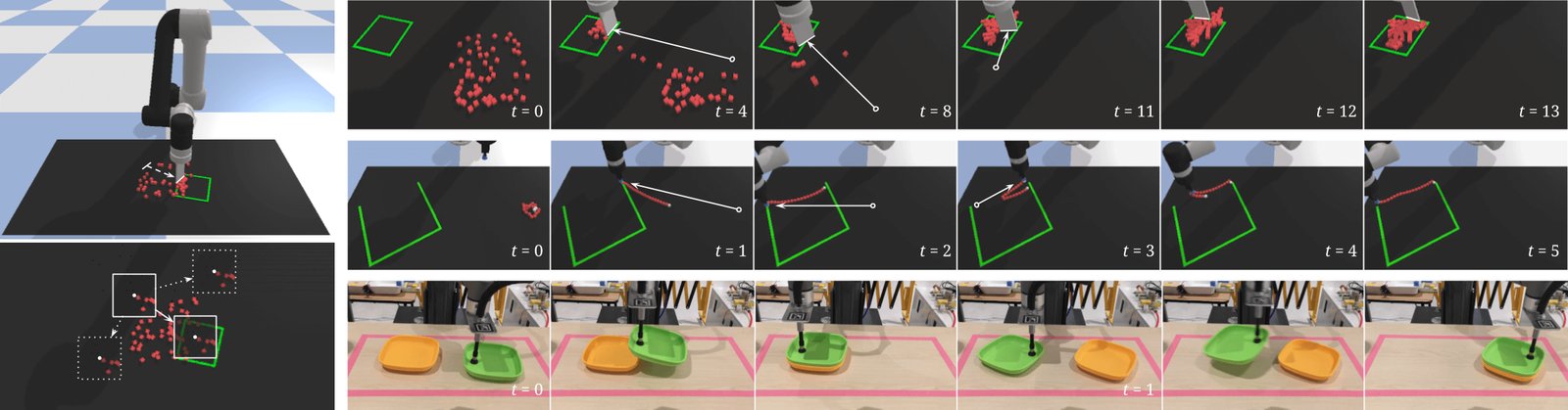
Figure 5: Transporter Networks can predict the desired spatial displacements of piles of small objects (left), which informs how to push them towards a target set. Our experiments show that it can learn visual feedback – enabling it to recover from mistakes (e.g., top row: pushing objects out of the target set at $t=11$), or sequentially rearrange a deformable rope (middle row). Since it learns pick-conditioned placing, it can also stack plates with varying initial predicted pick locations from only 10 demonstrations on a real robot (bottom row), without needing any object-specific representations.

图 5：Transporter Networks 可预测小物体堆的期望空间位移（左），从而指导如何把它们推向目标集合。实验表明它能学习视觉反馈——从而从错误中恢复（例如顶行：$t=11$ 时把物体推出目标集合），或依次重排可变形绳索（中行）。由于它学习以抓取为条件的放置，也能在真实机器人上仅用 10 条示范、在初始预测抓取位置变化的情况下叠放盘子（底行），而无需任何物体特定表示。

4.2 Real-World Experiments

4.2 真实世界实验

Task	Test %	# Samples
Mouthwash Kit Assembly	98.9	8141
Sweeping Piles of Go Pieces	98.3	6759

Table 5: Transporter Networks test performance on real robots with human demonstration data.

任务	测试 %	样本数
漱口水套件组装	98.9	8141
清扫围棋子堆	98.3	6759

表 5：Transporter Networks 在带人类示范数据的真实机器人上的测试表现。

We validate Transporter Networks on both the kit assembly and the sweeping tasks (shown in Fig. 1k and 1m) using real UR5e robots. For kit assembly, the robot uses a suction gripper and an industrial Photoneo PhoXi camera (for high resolution and accurate IR-depth). For sweeping, the robot uses a brush end effector and a low-cost consumer-grade Azure Kinect (for RGB-depth). Despite COVID-19 lockdowns preventing physical access, we were still able to perform real experiments using our Unity-based [46] UI that enables people to remotely teleoperate our robots to calibrate, collect training data, and run tests. For these experiments, teleoperators are tasked with i) repeatedly assembling and disassembling a kit of 5 bottled mouthwashes, or ii) sweeping piles of small Go pieces into a target goal zone marked with green tape, and autonomous resets using a scripted scrambling motion. Table 5 shows test performance of the models, and the amount of training data collected from 13 human operators in terms of transitions (i.e., pick and place actions for kit assembly, pushes for sweeping). We also show qualitative results of our robots in action for both tasks in our supplementary video. Further quantitative experiments were infeasible at time of submission due to COVID-19. Additional experiment details in the Appendix.

我们在真实 UR5e 机器人上验证 Transporter Networks 在套件组装与清扫任务上的表现（见图 1k 与 1m）。套件组装使用吸盘与工业级 Photoneo PhoXi 相机（高分辨率与精确 IR 深度）。清扫使用刷子末端与低成本消费级 Azure Kinect（RGB 深度）。尽管 COVID-19 封锁限制了现场接触，我们仍能用基于 Unity [46] 的界面远程遥操作机器人，完成标定、采集训练数据与跑测试。这些实验中，遥操作员的任务是 i）反复组装与拆卸装有 5 瓶漱口水的套件，或 ii）把小围棋子堆扫入用绿胶带标出的目标区，并用脚本化搅乱动作做自主复位。表 5 给出模型测试表现，以及 13 名人类操作员采集的训练数据量（以转移计，即套件组装的抓取放置动作、清扫的推动）。补充视频中还展示了两种任务上机器人动作的定性结果。因 COVID-19，投稿时进一步定量实验不可行。更多实验细节见附录。

5 Conclusion

5 结论

In this work, we presented the Transporter Network, a simple model architecture that infers spatial displacements, which can parameterize robot actions from visual input. It makes no assumptions of objectness, exploits spatial symmetries, and is orders of magnitude more sample efficient in learning vision-based manipulation tasks than end-to-end alternatives: from stacking a pyramid of blocks, to assembling kits with unseen objects, to pushing piles of small objects with closed-loop feedback. In terms of its current limitations: it is sensitive to camera-robot calibration, and it remains unclear how to integrate torque/force actions with spatial action spaces. Overall, we are excited about this direction and plan to extend it to real-time high-rate control, and as well as tasks involving tool use.

本文提出 Transporter Network，一种从视觉输入推断空间位移、并可据此参数化机器人动作的简洁模型结构。它不做物体性假设，利用空间对称性，在学习基于视觉的操作任务上样本效率比端到端替代方案高出数个数量级：从堆叠积木金字塔，到用未见物体组装套件，再到用闭环反馈推动小物体堆。就当前局限而言：它对相机—机器人标定敏感，且尚不清楚如何把力矩/力动作与空间动作空间结合。总体而言，我们对这一方向感到兴奋，并计划扩展到实时高速率控制，以及涉及工具使用的任务。

Acknowledgments

Special thanks to Ken Goldberg, Razvan Surdulescu, Daniel Seita, Ayzaan Wahid, Vincent Vanhoucke, Anelia Angelova, for helpful feedback on writing, Sean Snyder, Jonathan Vela, Larry Bisares, Michael Villanueva, Brandon Hurd for operations and hardware support, Robert Baruch for software infrastructure, Jared Braun for UI contributions, Erwin Coumans for PyBullet advice, Laura Graesser for video narration.

致谢

Special thanks to Ken Goldberg, Razvan Surdulescu, Daniel Seita, Ayzaan Wahid, Vincent Vanhoucke, Anelia Angelova, for helpful feedback on writing, Sean Snyder, Jonathan Vela, Larry Bisares, Michael Villanueva, Brandon Hurd for operations and hardware support, Robert Baruch for software infrastructure, Jared Braun for UI contributions, Erwin Coumans for PyBullet advice, Laura Graesser for video narration.

References

Levine et al. [2016] S. Levine, C. Finn, T. Darrell, and P. Abbeel. End-to-end training of deep visuomotor policies. The Journal of Machine Learning Research (JMLR) , 2016.

Kalashnikov et al. [2018] D. Kalashnikov, A. Irpan, P. Pastor, J. Ibarz, A. Herzog, E. Jang, D. Quillen, E. Holly, M. Kalakrishnan, V. Vanhoucke, et al. Qt-opt: Scalable deep reinforcement learning for vision-based robotic manipulation. Conference on Robot Learning (CoRL) , 2018.

Manuelli et al. [2019] L. Manuelli, W. Gao, P. Florence, and R. Tedrake. kpam: Keypoint affordances for category-level robotic manipulation. International Symposium on Robotics Research (ISRR) , 2019.

Kulkarni et al. [2019] T. D. Kulkarni, A. Gupta, C. Ionescu, S. Borgeaud, M. Reynolds, A. Zisserman, and V. Mnih. Unsupervised learning of object keypoints for perception and control. NeurIPS , 2019.

Nagabandi et al. [2020] A. Nagabandi, K. Konolige, S. Levine, and V. Kumar. Deep dynamics models for learning dexterous manipulation. Conference on Robot Learning (CoRL) , 2020.

Liu et al. [2020] X. Liu, R. Jonschkowski, A. Angelova, and K. Konolige. Keypose: Multi-view 3d labeling and keypoint estimation for transparent objects. IEEE Conference on Computer Vision and Pattern Recognition (CVPR) , 2020.

Mees et al. [2017] O. Mees, N. Abdo, M. Mazuran, and W. Burgard. Metric learning for generalizing spatial relations to new objects. IEEE/RSJ International Conference on Intelligent Robots and Systems (IROS) , 2017.

Jund et al. [2018] P. Jund, A. Eitel, N. Abdo, and W. Burgard. Optimization beyond the convolution: Generalizing spatial relations with end-to-end metric learning. IEEE International Conference on Robotics and Automation (ICRA) , 2018.

Florence et al. [2018] P. R. Florence, L. Manuelli, and R. Tedrake. Dense object nets: Learning dense visual object descriptors by and for robotic manipulation. Conference on Robot Learning (CoRL) , 2018.

Florence et al. [2019] P. Florence, L. Manuelli, and R. Tedrake. Self-supervised correspondence in visuomotor policy learning. IEEE Robotics and Automation Letters (RA-L) , 2019.

Sundaresan et al. [2020] P. Sundaresan, J. Grannen, B. Thananjeyan, A. Balakrishna, M. Laskey, K. Stone, J. E. Gonzalez, and K. Goldberg. Learning rope manipulation policies using dense object descriptors trained on synthetic depth data. IEEE International Conference on Robotics and Automation (ICRA) , 2020.

Suh and Tedrake [2020] H. Suh and R. Tedrake. The surprising effectiveness of linear models for visual foresight in object pile manipulation. Workshop on Algorithmic Foundations of Robotics (WAFR) , 2020.

Kondor and Trivedi [2018] R. Kondor and S. Trivedi. On the generalization of equivariance and convolution in neural networks to the action of compact groups. International Conference on Machine Learning (ICML) , 2018.

Cohen and Welling [2016] T. Cohen and M. Welling. Group equivariant convolutional networks. International Conference on Machine Learning (ICML) , 2016.

Platt et al. [2019] R. Platt, C. Kohler, and M. Gualtieri. Deictic image mapping: An abstraction for learning pose invariant manipulation policies. AAAI Conference on Artificial Intelligence , 2019.

Brockman et al. [2016] G. Brockman, V. Cheung, L. Pettersson, J. Schneider, J. Schulman, J. Tang, and W. Zaremba. Openai gym. arXiv preprint arXiv:1606.01540 , 2016.

Yoon et al. [2003] Y. Yoon, G. N. DeSouza, and A. C. Kak. Real-time tracking and pose estimation for industrial objects using geometric features. IEEE International Conference on Robotics and Automation (ICRA) , 2003.

Zhu et al. [2014] M. Zhu, K. G. Derpanis, Y. Yang, S. Brahmbhatt, M. Zhang, C. Phillips, M. Lecce, and K. Daniilidis. Single image 3d object detection and pose estimation for grasping. ICRA , 2014.

Zeng et al. [2017] A. Zeng, K.-T. Yu, S. Song, D. Suo, E. Walker, A. Rodriguez, and J. Xiao. Multi-view self-supervised deep learning for 6d pose estimation in the amazon picking challenge. IEEE International Conference on Robotics and Automation (ICRA) , 2017.

Deng et al. [2020] X. Deng, Y. Xiang, A. Mousavian, C. Eppner, T. Bretl, and D. Fox. Self-supervised 6d object pose estimation for robot manipulation. IEEE International Conference on Robotics and Automation (ICRA) , 2020.

Wang et al. [2019] H. Wang, S. Sridhar, J. Huang, J. Valentin, S. Song, and L. J. Guibas. Normalized object coordinate space for category-level 6d object pose and size estimation. Computer Vision and Pattern Recognition (CVPR) , 2019.

Frazzoli et al. [2005] E. Frazzoli, M. A. Dahleh, and E. Feron. Maneuver-based motion planning for nonlinear systems with symmetries. IEEE Transactions on Robotics (T-RO) , 2005.

Gualtieri et al. [2018] M. Gualtieri, A. ten Pas, and R. Platt. Pick and place without geometric object models. IEEE International Conference on Robotics and Automation (ICRA) , 2018.

Zakka et al. [2020] K. Zakka, A. Zeng, J. Lee, and S. Song. Form2fit: Learning shape priors for generalizable assembly from disassembly. IEEE International Conference on Robotics and Automation (ICRA) , 2020.

Hundt et al. [2020] A. Hundt, B. Killeen, N. Greene, H. Wu, H. Kwon, C. Paxton, and G. D. Hager. “good robot!”: Efficient reinforcement learning for multi-step visual tasks with sim to real transfer. IEEE Robotics and Automation Letters (RA-L) , 2020.

Berscheid et al. [2020] L. Berscheid, P. Meißner, and T. Kröger. Self-supervised learning for precise pick-and-place without object model. IEEE Robotics and Automation Letters (RA-L) , 2020.

Wu et al. [2020] Y. Wu, W. Yan, T. Kurutach, L. Pinto, and P. Abbeel. Learning to manipulate deformable objects without demonstrations. Robotics: Science and Systems (RSS) , 2020.

Devin et al. [2020] C. Devin, P. Rowghanian, C. Vigorito, W. Richards, and K. Rohanimanesh. Self-supervised goal-conditioned pick and place. arXiv preprint arXiv:2008.11466 , 2020.

Khansari et al. [2020] M. Khansari, D. Kappler, J. Luo, J. Bingham, and M. Kalakrishnan. Action image representation: Learning scalable deep grasping policies with zero real world data. IEEE International Conference on Robotics and Automation (ICRA) , 2020.

Song et al. [2020] S. Song, A. Zeng, J. Lee, and T. Funkhouser. Grasping in the wild: Learning 6dof closed-loop grasping from low-cost demonstrations. IEEE Robotics and Automation Letters (RA-L) , 2020.

Zeng et al. [2018] A. Zeng, S. Song, K.-T. Yu, E. Donlon, F. R. Hogan, M. Bauza, D. Ma, O. Taylor, M. Liu, E. Romo, et al. Robotic pick-and-place of novel objects in clutter with multi-affordance grasping and cross-domain image matching. International Conference on Robotics and Automation (ICRA) , 2018.

Morrison et al. [2018] D. Morrison, P. Corke, and J. Leitner. Closing the loop for robotic grasping: A real-time, generative grasp synthesis approach. Robotics: Science and Systems (RSS) , 2018.

Zeng et al. [2018] A. Zeng, S. Song, S. Welker, J. Lee, A. Rodriguez, and T. Funkhouser. Learning synergies between pushing and grasping with self-supervised deep reinforcement learning. IEEE/RSJ International Conference on Intelligent Robots and Systems (IROS) , 2018.

Long et al. [2015] J. Long, E. Shelhamer, and T. Darrell. Fully convolutional networks for semantic segmentation. IEEE Conference on Computer Vision and Pattern Recognition (CVPR) , 2015.

[35] A. Zeng. Learning Visual Affordances for Robotic Manipulation . PhD thesis, Princeton University.

Li et al. [2019] B. Li, W. Wu, Q. Wang, F. Zhang, J. Xing, and J. Yan. Siamrpn++: Evolution of siamese visual tracking with very deep networks. Conference on Computer Vision and Pattern Recognition , 2019.

Bertinetto et al. [2016] L. Bertinetto, J. Valmadre, J. F. Henriques, A. Vedaldi, and P. H. Torr. Fully-convolutional siamese networks for object tracking. European Conference on Computer Vision (ECCV) , 2016.

Tao et al. [2016] R. Tao, E. Gavves, and A. W. Smeulders. Siamese instance search for tracking. IEEE Conference on Computer Vision and Pattern Recognition (CVPR) , 2016.

Luo et al. [2016] W. Luo, Y. Li, R. Urtasun, and R. Zemel. Understanding the effective receptive field in deep convolutional neural networks. Advances in Neural Information Processing Systems (NeurIPS) , 2016.

Seita et al. [2020] D. Seita, P. Florence, J. Tompson, E. Coumans, V. Sindhwani, K. Goldberg, and A. Zeng. Learning to rearrange deformable cables, fabrics, and bags with goal-conditioned transporter networks. arXiv preprint arXiv:2012.03385 , 2020.

He et al. [2016] K. He, X. Zhang, S. Ren, and J. Sun. Deep residual learning for image recognition. IEEE Conference on Computer Vision and Pattern Recognition (CVPR) , 2016.

Yu and Koltun [2016] F. Yu and V. Koltun. Multi-scale context aggregation by dilated convolutions. International Conference on Learning Representations , 2016.

Nair and Hinton [2010] V. Nair and G. E. Hinton. Rectified linear units improve restricted boltzmann machines. International Conference on Machine Learning (ICML) , 2010.

Coumans and Bai [2016] E. Coumans and Y. Bai. Pybullet, a python module for physics simulation for games, robotics and machine learning. GitHub Repository , 2016.

Bishop [1994] C. M. Bishop. Mixture density networks. Aston University , 1994.

Unity Technologies [Version: 2018.4.0f1] Unity Technologies. Unity game engine. Version: 2018.4.0f1. URL https://unity.com .

Schmidt et al. [2016] T. Schmidt, R. Newcombe, and D. Fox. Self-supervised visual descriptor learning for dense correspondence. IEEE Robotics and Automation Letters (RA-L) , 2016.

Goroshin et al. [2015] R. Goroshin, M. F. Mathieu, and Y. LeCun. Learning to linearize under uncertainty. Advances in Neural Information Processing Systems (NeurIPS) , 2015.

Szegedy et al. [2015] C. Szegedy, W. Liu, Y. Jia, P. Sermanet, S. Reed, D. Anguelov, D. Erhan, V. Vanhoucke, and A. Rabinovich. Going deeper with convolutions. IEEE Conference on Computer Vision and Pattern Recognition (CVPR) , 2015.

Rahmatizadeh et al. [2018] R. Rahmatizadeh, P. Abolghasemi, L. Bölöni, and S. Levine. Vision-based multi-task manipulation for inexpensive robots using end-to-end learning from demonstration. ICRA , 2018.

Mildenhall et al. [2020] B. Mildenhall, P. P. Srinivasan, M. Tancik, J. T. Barron, R. Ramamoorthi, and R. Ng. Nerf: Representing scenes as neural radiance fields for view synthesis. European Conference on Computer Vision (ECCV) , 2020.

Sitzmann et al. [2020] V. Sitzmann, J. N. Martel, A. W. Bergman, D. B. Lindell, and G. Wetzstein. Implicit neural representations with periodic activation functions. Advances in Neural Information Processing Systems (NeurIPS) , 2020.

Kingma and Ba [2015] D. P. Kingma and J. Ba. Adam: A method for stochastic optimization. International Conference on Learning Representations (ICLR) , 2015.

6 Appendix

6 附录

The appendix consists of: descriptions of tasks and evaluation metrics in the Ravens simulation framework, additional experimental results, analysis, ablation studies, and real system details.

附录包括：Ravens 仿真框架中的任务与评估指标描述、额外实验结果、分析、消融研究，以及真实系统细节。

6.1 Simulation Experimentation, Real World Experimentation, and COVID-19

6.1 仿真实验、真实世界实验与 COVID-19

As introduced in the main paper, we execute experiments in simulation with Ravens as a means to provide a consistent environment for comparisons to baselines and ablations. Models evaluated in simulation are trained only on simulated data. Likewise models evaluated in the real-world are trained only on real data. In simulation, we avoid assumptions that cannot transfer to a real setup: observation data contains only 640x480 RGB-D images and camera parameters; actions are end effector poses (transposed into joint positions with inverse kinematics). The only exception to this is our GT-State baseline, which learns MLPs that take ground truth state information (e.g., object poses, bounding boxes, and color) as input – shown to be less sample efficient than Transporter Networks for many tasks. A limitation of Ravens is that the rendering software stack may not fully reflect the noise characteristics often found in real data: inaccuracies in camera calibration (e.g., intrinsics and extrinsics), noise in commodity depth sensors. Hence, we also test our method on a real system (details in Sec. 6.14) using teleoperated demonstration data, and present qualitative results in our supplementary video. Extensive quantitative experiments on real robots was difficult due to limited physical access during COVID-19.

如正文所述，我们用 Ravens 做仿真实验，以便为与基线及消融的对照提供一致环境。仿真中评估的模型只在仿真数据上训练；真实世界评估的模型只在真实数据上训练。仿真中我们避免无法迁移到真实设定的假设：观测数据仅含 640×480 RGB-D 图像与相机参数；动作为末端执行器位姿（经逆运动学转为关节位置）。唯一例外是 GT-State 基线，它学习以真实状态信息（例如物体位姿、包围盒与颜色）为输入的 MLP——在许多任务上显示样本效率低于 Transporter Networks。Ravens 的局限是渲染软件栈可能无法完全反映真实数据中常见的噪声特性：相机标定不准（例如内外参）、消费级深度传感器噪声。因此我们也在真实系统上测试方法（细节见第 6.14 节），使用遥操作示范数据，并在补充视频中给出定性结果。因 COVID-19 期间现场接触有限，真实机器人上的大规模定量实验较为困难。

6.2 Ravens Simulation Framework

6.2 Ravens 仿真框架

In our simulation framework, Ravens, each task comes with a scripted oracle that provides expert demonstrations by randomly sampling the distribution of successful picking and placing actions – samples of which are made available to the learner. Ravens also has several attributes that make it useful for studying different areas that are beyond the scope of this work, including: 1) active learning, since algorithms can query an oracle during specific moments of uncertainty to improve learning efficiency, 2) reinforcement learning, since we provide reward functions that provide partial credit for all tasks (used only for evaluation in this work), and 3) active perception, since camera parameters (e.g., extrinsics) are defined by an action (static in our experiments, but could be dynamic), which provides an opportunity to study algorithms that improve learning through active control of the camera position and orientation.

在仿真框架 Ravens 中，每项任务配有脚本 oracle，通过随机采样成功抓取与放置动作的分布提供专家示范——其中样本提供给学习者。Ravens 还有若干属性，使其适合研究超出本文范围的其他方向，包括：1）主动学习，因为算法可在不确定时刻查询 oracle 以提高学习效率；2）强化学习，因为我们为所有任务提供给出部分分的奖励函数（本文仅用于评估）；3）主动感知，因为相机参数（例如外参）由动作定义（我们实验中为静态，但可以是动态的），从而有机会研究通过主动控制相机位姿改善学习的算法。

During both training and testing, all objects (including target zones) are randomly positioned and oriented in the workspace. To succeed in the case where only a single demonstration is provided, the learner needs to be invariant to unseen configurations of objects. Information about the multi-modality of a task or its sequential permutations is only made available from the distribution of demonstrations. For example, moving disks in Towers of Hanoi may have only one correct sequence of states, but the distribution of how each disk can be picked or placed is learned from multiple demonstrations. Or, when palletizing homogeneous boxes, the arrangement of boxes across each layer on the pallet must be transposed, and boxes should be stacked stably on top other boxes already on the stack to avoid toppling. In our experiments, Transporter Networks are trained from scratch, without any pre-training from vision datasets. Exploring multi-task training for more efficient generalization to new tasks is interesting future work.

训练与测试时，所有物体（含目标区域）在工作空间中随机位姿。当只提供单条示范时，学习者需要对未见物体构型保持不变性。关于任务多峰性或其序列置换的信息，只从示范分布中获得。例如，河内塔中移动圆盘可能只有一条正确状态序列，但每个圆盘如何被抓取或放置的分布要从多条示范中学习。或者，在码垛同类纸箱时，托盘每层纸箱排列必须交错，且纸箱应稳定地叠在已有纸箱之上以免倒塌。实验中 Transporter Networks 从零训练，不使用视觉数据集预训练。探索多任务训练以更高效泛化到新任务，是有趣的未来工作。

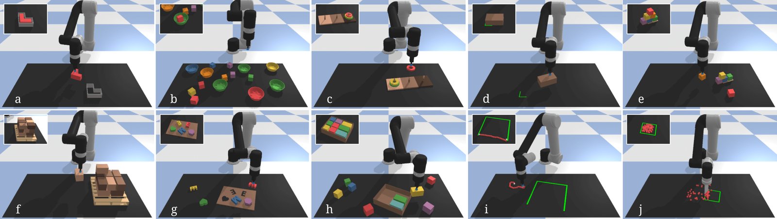
Figure 6: Tasks: (row-major order) block-insertion, place-red-in-green, towers-of-hanoi, align-box-corner, stack-block-pyramid, palletizing-boxes, assembling-kits, packing-boxes, manipulating-rope, sweeping-piles. Goal states (not provided to learners) are shown in top left corner of each image.

图 6：任务：（行优先）block-insertion、place-red-in-green、towers-of-hanoi、align-box-corner、stack-block-pyramid、palletizing-boxes、assembling-kits、packing-boxes、manipulating-rope、sweeping-piles。目标状态（不提供给学习者）显示在每张图像左上角。

6.3 Ravens-10 Benchmark Task Details

6.3 Ravens-10 基准任务细节

A set of 10 tasks (illustrated in Fig. 6) comprise our Ravens-10 benchmark. In each of these tasks, the agent acts with motion primitives parameterized by a sequence of two SE(2) end effector poses. Note that although the two motion-primitive-defining poses are in SE(2), manipulation behaviors that are in 3D can still be achieved (such as stacking blocks on top of each other) due to motion primitives that involve out-of-plane movement.

一组 10 项任务（见图 6）构成我们的 Ravens-10 基准。在每项任务中，智能体用由两个 SE(2) 末端位姿参数化的运动基元动作序列行动。注意尽管定义运动基元的两个位姿在 SE(2) 中，仍可实现三维中的操作行为（例如把积木叠在彼此之上），因为运动基元可包含平面外运动。

block-insertion: picking up an L-shaped red block and placing it into an L-shaped fixture with a corresponding hole. The block is 8cm in diameter while the hole is 9cm in diameter. The block and fixture configurations are randomly sampled in the workspace – rejected if in collision with each other, or if partially out of bounds in the workspace.

block-insertion： 拿起 L 形红色积木，放入带对应孔洞的 L 形夹具。积木直径 8 cm，孔洞直径 9 cm。积木与夹具构型在工作空间中随机采样——若彼此碰撞，或部分超出工作空间边界则拒绝。

place-red-in-green: picking up red blocks and placing them into green bowls amidst other visually distracting objects (e.g., randomly positioned blocks and bowls of different colors). There can be multiple red blocks and/or multiple green bowls, with a random chance for more bowls than blocks. This task requires handling multiple candidate picking and placing locations. Since bowls are twice as large as the blocks, this task does not require precision. Red blocks and green bowls are first added to the workspace, then 10 objects (blocks or bowls of other colors) are randomly spawned in collision-free configurations.

place-red-in-green： 在其他视觉干扰物体（例如不同颜色的随机位姿积木与碗）中间，拿起红色积木放入绿色碗。可有多个红色积木和/或多个绿色碗，并有随机概率使碗多于积木。该任务需要处理多个候选抓取与放置位置。由于碗大约是积木两倍大，该任务不要求高精度。先将红色积木与绿色碗加入工作空间，再随机无碰撞地生成 10 个物体（其他颜色的积木或碗）。

towers-of-hanoi: sequentially picking up disks and placing them into pegs such that all 3 disks initialized on one peg are moved to another, and that only smaller disks can be on top of larger ones. Completing this task requires sequencing 7 pick-and-places of the disks in a specific order. During evaluation, no information about which disk should be picked next is provided – the approach needs to infer this from contextual visual cues e.g., the positions or absence (due to occlusions) of other disks. This tests the capacity of the learner to infer the sequential semantics of Markovian vision-based manipulation tasks. Fig. 7 illustrates this task, its ground truth sequence, picking action distribution, and placing action distributions (unimodal for translation-only placing, or spiral shaped for the SE(2) placing). The base of the 3 pegs are randomly configured in the workspace, and disks are initialized on the peg on the lightest side of the base.

towers-of-hanoi： 依次拿起圆盘放入柱子，使初始化在一根柱上的 3 个圆盘移到另一根，且只有较小圆盘可叠在较大圆盘上。完成该任务需要按特定顺序对圆盘做 7 次抓取放置。评估时不提供下一步应抓哪个圆盘的信息——方法需从上下文视觉线索推断，例如其他圆盘的位置或因遮挡而缺失。这检验学习者推断马尔可夫视觉操作任务序列语义的能力。图 7 展示该任务、其真实序列、抓取动作分布，以及放置动作分布（仅平移放置为单峰，或 SE(2) 放置为螺旋形）。三根柱的底座在工作空间中随机配置，圆盘初始化在底座最浅色一侧的柱上。

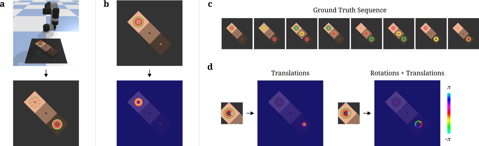
Figure 7: In Towers of Hanoi (a), the task is to sequentially pick-and-place 3 disks from the first peg to the third peg without placing a larger disk over a smaller disk (c). In each step, the distribution of successful picks is ring-shaped (b), and the distribution of successful pick-conditioned placements (d) is unimodal with translation-only placing, or spiral-shaped with SE(2) placing (projected onto a ring for visualization, where the ring traverses different rotations). The nature of this task evaluates the capacity of Transporter Networks to recover non-trivial spatial action distributions, and to sequence actions by leveraging contextual visual cues.

图 7：在河内塔 (a) 中，任务是依次把 3 个圆盘从第一柱抓取放置到第三柱，且不能把大盘放在小盘上 (c)。每一步，成功抓取分布呈环形 (b)，以抓取为条件的成功放置分布 (d) 在仅平移放置时为单峰，在 SE(2) 放置时为螺旋形（投影到环上以便可视化，环遍历不同旋转）。该任务性质评估 Transporter Networks 恢复非平凡空间动作分布、以及利用上下文视觉线索对动作排序的能力。

align-box-corner: picking up a randomly sized box and repositioning it on the tabletop to align one of its corners to a green L-shaped marker labeled on the tabletop. This task requires precision, and the ability to generalize to new box sizes. Aligning any of the box’s corners to the green marker yields task success. The marker and box are randomly configured in the workspace such that the box does not overlap the marker.

align-box-corner： 拿起随机尺寸的盒子，在桌面上重定位，使其一角与桌面上标记的绿色 L 形标记对齐。该任务要求精度，以及泛化到新盒子尺寸的能力。盒子任意一角对齐绿色标记即算任务成功。标记与盒子在工作空间中随机配置，使盒子不与标记重叠。

stack-block-pyramid: sequentially picking up 6 blocks (each with a different color) and stacking them into a pyramid of 3-2-1. The bottom 3 blocks can only be purple, green, or blue blocks. The middle 2 blocks can only be orange or yellow blocks. The top block can only be red. A successful pyramid is invariant to the permutation of blocks within each row, but not between rows. The blocks and base of the pyramid are randomly spawned in collision-free configurations.

stack-block-pyramid： 依次拿起 6 块不同颜色的积木，堆成 3-2-1 的金字塔。底部 3 块只能是紫、绿或蓝；中间 2 块只能是橙或黄；顶块只能是红。成功金字塔对每行内积木置换不变，但对行间置换不变。积木与金字塔底座以无碰撞构型随机生成。

palletizing-boxes: picking up fixed-sized boxes and stacking them on top of a pallet. To mimic real stability constraints, the arrangement of boxes should be transposed across each layer of the pallet. There are a fixed number of boxes – each one is spawned into the workspace prior to each pick-and-place action.

palletizing-boxes： 拿起固定尺寸纸箱并堆叠到托盘上。为模拟真实稳定性约束，托盘每层纸箱排列应交错。纸箱数量固定——每次抓取放置前向工作空间生成一个。

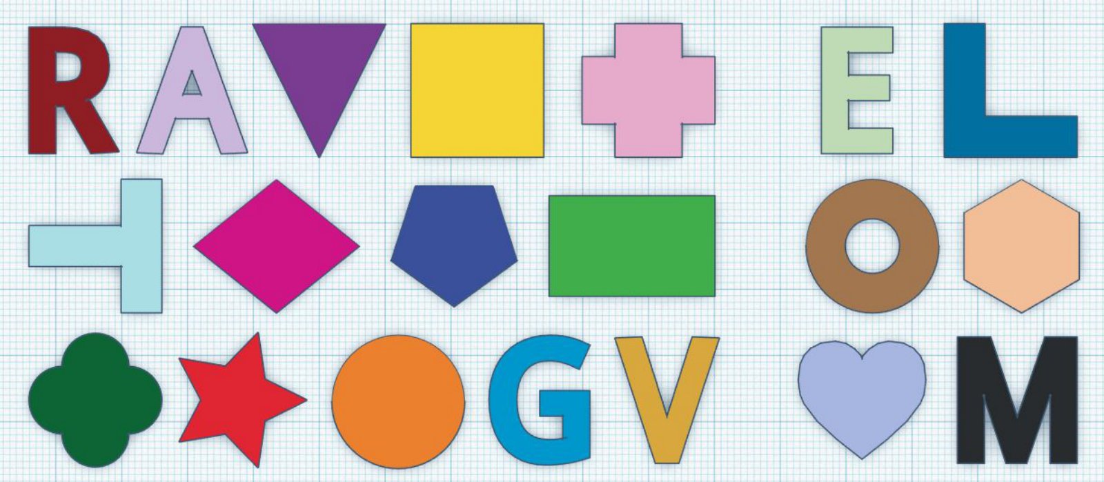
Figure 8: Kitting objects used in training (left 14) and testing (right 6).

图 8：训练使用的套件物体（左 14 个）与测试使用的物体（右 6 个）。

assembling-kits: picking and placing different shaped objects onto corresponding locations on a board (visually marked with corresponding silhouettes of the objects). For each episode, 5 objects are randomly selected with replacement from a set of 20: 14 used during training (left), and 6 held out for testing (right). This task requires precise placing and generalizing to new objects by learning the concept of ”how things fit together” [24]. The kit and 5 objects are randomly spawned in collision-free configurations.

assembling-kits： 把不同形状物体抓取放置到板上对应位置（用物体轮廓视觉标记）。每回合有放回地从 20 个物体集合中随机选 5 个：14 个用于训练（左），6 个留作测试（右）。该任务需要精确放置，并通过学习「物体如何拼合」的概念泛化到新物体 [24]。套件与 5 个物体以无碰撞构型随机生成。

packing-boxes: picking and placing randomly sized boxes tightly into a randomly sized container. This task is the hardest one in the benchmark, which requires not only relying on visual cues to tightly fit objects together, but also implicitly learning to order the objects in ways that maximize container coverage. During initialization, the container size is first randomly sampled, then randomly partitioned using a binary search tree (with minimum size of 5cm along each dimension). Each partition then parameterizes the size of each box, individually spawned into the workspace with a collision-free configuration.

packing-boxes： 把随机尺寸纸箱紧密放入随机尺寸容器。这是基准中最难的任务，不仅需要依赖视觉线索把物体紧密拼合，还要隐式学习以最大化容器覆盖的方式对物体排序。初始化时先随机采样容器尺寸，再用二叉搜索树随机划分（每维最小 5 cm）。每个划分再参数化每个纸箱尺寸，并各自以无碰撞构型生成到工作空间。

manipulating-rope: manipulating a deformable rope such that it connects the two endpoints of an incomplete 3-sided square (colored in green). The cable is initialized as a randomly formed pile in the workspace, which needs to be untangled then aligned with the square. This task requires sequencing actions with closed-loop visual feedback to incrementally adjust the rope. The rope is implemented as a set of 20 articulated spherical beads, randomly dropped onto the workspace. The 3-sided square is randomly configured in the workspace.

manipulating-rope： 操作可变形绳索，使其连接不完整三边正方形（绿色）的两端点。绳索初始化为工作空间中随机形成的一堆，需要先理顺再与正方形对齐。该任务需要用闭环视觉反馈对动作排序，以增量调整绳索。绳索实现为 20 个铰接球形珠，随机落到工作空间。三边正方形在工作空间中随机配置。

sweeping-piles: pushing piles of small objects (randomly initialized) into a desired target goal zone on the tabletop marked with green boundaries. This sequential task (inspired by [12]) requires sequencing pushes with closed-loop visual feedback and handling piles of small objects. In this task, the suction end effector is swapped with a spatula. The small objects and the target goal zone are randomly initialized in the workspace.

sweeping-piles： 把随机初始化的小物体堆推入桌面上用绿色边界标出的目标区。这一序列任务（受 [12] 启发）需要用闭环视觉反馈对推动排序，并处理小物体堆。该任务中吸盘末端换成铲子。小物体与目标区在工作空间中随机初始化。

6.4 Additional Tasks

6.4 额外任务

In addition to the Ravens-10 tasks, we used two other tasks in the paper for analysis. The first was to provide a simplified test environment for testing the difference between stochastic and deterministic demonstrations (Sec. 4), and interpolation/extrapolation experiments with a small enough amount of degrees of freedom such that they could be plotted (Sec. 6.10). The second task was to test the SE(3) variant of Transporter Networks.

除 Ravens-10 任务外，我们还在文中用了另外两项任务做分析。第一项提供简化测试环境，用于检验随机与确定性示范的差异（第 4 节），以及自由度足够少以便绘图的插值/外推实验（第 6.10 节）。第二项用于测试 Transporter Networks 的 SE(3) 变体。

2DoF simplified block-insertion: This task is identical to the block-insertion task, except: (i) the block is always in the same staring configuration, and (ii) the fixture varies only in translation. The environment initialization has 2 degrees of freedom total.

二维自由度简化积木插入： 该任务与 block-insertion 相同，除了：(i) 积木始终处于同一起始构型；(ii) 夹具仅在平移上变化。环境初始化共有 2 个自由度。

6DoF block insertion: This task is identical to the block-insertion task, except that the fixture varies in 6 degrees of freedom, requiring SE(3) placing. In addition to the table-plane degrees of freedom, the fixture also varies in height ($z$) as well as the two rotational degrees of freedom out of the plane, which may be represented by roll and pitch. The block varies only in SE(2). The environment initialization has 9 degrees of freedom total.

六自由度积木插入： 该任务与 block-insertion 相同，但夹具在 6 个自由度上变化，需要 SE(3) 放置。除桌面平面自由度外，夹具还在高度（$z$）以及平面外两个旋转自由度上变化，可用 roll 与 pitch 表示。积木仅在 SE(2) 上变化。环境初始化共有 9 个自由度。

6.5 Evaluation Metrics

6.5 评估指标

Performance on each task in simulation is evaluated in one of two ways:

仿真中每项任务的性能用以下两种方式之一评估：

Pose: object translation and rotation to target pose is less than a threshold $\tau=1$cm and $\omega=15^{\circ}$ respectively. If completing a task requires sequencing multiple actions, then each successful action (where an object is moved to its correct pose) returns a partial reward $r=\frac{1}{\textrm{\# of actions}}$. Total rewards for completing a task always sums to 1. Object symmetries are accounted for. Tasks: block-insertion, towers-of-hanoi, place-red-in-green, align-box-corner, stack-block-pyramid, assembling-kits.

位姿： 物体相对目标位姿的平移与旋转分别小于阈值 $\tau=1$ cm 与 $\omega=15^{\circ}$。若完成任务需要排序多个动作，则每次成功动作（物体被移到正确位姿）返回部分奖励 $r=\frac{1}{\textrm{\# of actions}}$。完成任务的总奖励始终和为 1。已考虑物体对称性。任务：block-insertion、towers-of-hanoi、place-red-in-green、align-box-corner、stack-block-pyramid、assembling-kits。

Zone: ratio of object(s) in the target zone. We discretize each object’s 3D bounding box into 2cm3 voxels. Total reward is the fraction of total voxels in the target zone $r=\frac{\textrm{\# of voxels in target zone}}{\textrm{total \# of voxels}}$. Tasks: palletizing-boxes, packing-boxes, manipulating-cables, sweeping-piles. Achieving total reward $r=1$ on palletizing-boxes and packing-boxes requires tightly fitting all objects into the target zone (i.e., it is exponentially more difficult to achieve $r=0.9$ than it is to achieve the first $r=0.5$).

区域： 物体在目标区内的比例。我们将每个物体的三维包围盒离散为 2 cm³ 体素。总奖励是目标区内体素占总体素数的比例 $r=\frac{\textrm{\# of voxels in target zone}}{\textrm{total \# of voxels}}$。任务：palletizing-boxes、packing-boxes、manipulating-cables、sweeping-piles。在 palletizing-boxes 与 packing-boxes 上达到总奖励 $r=1$ 需要把所有物体紧密放入目标区（即达到 $r=0.9$ 比达到最初的 $r=0.5$ 指数级更难）。

6.6 Data Augmentation

6.6 数据增强

As is common with deep learning methods, we find that data augmentation can substantially benefit generalization performance for Transporter Nets. To control the experimental comparisons with baselines in this paper, all methods used an identical data augmentation distribution. Specifically, a random SE(2) transform, $T^{aug}_{\mathcal{W}}$, relative to the world frame $\mathcal{W}$ was sampled, and all observations (whether the images, or the object poses for the GT-State methods) were adjusted as if the data was observed from the augmentation frame $aug$ rather than the world frame. This augmentation makes the assumption that the absolute position of objects on the table plane does not matter for the tasks – this was indeed the case for all tasks shown. Note that this distribution provides augmentation along the 3 degrees of freedom of SE(2), but we do not apply other augmentations such as imagining different relative configurations of objects – this would not be a feasible assumption for certain tasks that involve multiple objects.

与深度学习方法常见做法一样，我们发现数据增强能显著提升 Transporter Nets 的泛化表现。为控制本文与基线的实验对照，全部方法使用相同的数据增强分布。具体地，相对世界系 $\mathcal{W}$ 采样随机 SE(2) 变换 $T^{aug}_{\mathcal{W}}$，并将所有观测（无论是图像，还是 GT-State 方法的物体位姿）调整为仿佛从增强系 $aug$ 而非世界系观测到的数据。该增强假设桌面平面上物体的绝对位置对任务无关——所示全部任务确实如此。注意该分布沿 SE(2) 的 3 个自由度提供增强，但我们不施加其他增强，例如想象物体不同相对构型——对涉及多物体的某些任务，这不是可行假设。

6.7 Additional Baseline Details

6.7 额外基线细节

Form2Fit [24] is a recent method for pick-and-place (also similar to Devin et al. [28]), using a matching network that computes dense visual descriptors [9, 47] to associate picking actions to placing actions. We use an author-provided implementation of Form2Fit with 43-layer ResNet backbones of similar parameter count for a fair comparison.

Form2Fit [24] 是较新的抓取放置方法（也类似 Devin 等人 [28]），用匹配网络计算稠密视觉描述子 [9, 47] 以关联抓取动作与放置动作。我们使用作者提供的 Form2Fit 实现，采用参数量相近的 43 层 ResNet 骨干以便公平对照。

ConvMLP is a model architecture first proposed in [1] for learning control policies from pixel input – commonly used in end-to-end literature. While typically this architecture is used for real-time continuous control and was originally used with a joint torque action space, we tried it here for our motion-primitive-based setting with a spatial action space. The input images are the same as that of Transporter Networks and Form2Fit: top-down reconstructed views from RGB-D data. The architecture consists of a series of three convolutional layers, followed by spatial soft(arg)max [48] and a multi-layer perceptron to regress a 6-dimensional vector of the two SE(2) end-effector poses. The architecture used was almost exactly as in [1], but with the following changes: (i) we used channel depths of 64, 64, 64, rather than the 64, 32, 16 used in the original paper, (ii) we used MLP layer widths of 128, 128, (iii) we used the MLP to regress mixture densities [45] rather than direct regression in order to handle multi-modality, and (iv) we added depth image input to the network, by replicating depth along 3 channels, processing it with one separate 7x7 convolutional layer, and then fusing with RGB after the first layer via concatenation. The addition of depth image input into the model was to be more directly comparable with the other image-based options, which also used depth. As in [1], we use ImageNet-pretrained weights from GoogLeNet [49] for the first RGB convolutional layer, which we find to aid in stable training and generalization. While this network is 10x shallower (3 layers) than the network used for Form2Fit and Transporter Nets (43 layers), we tried to train the same 43-layer backbone network used in Transporter Networks with a spatial soft(arg)max and MLP, but found that the shallower 3-layer network achieved better generalization at least for our tested hyperparameters. Since many tasks involved multi-modal policies, it was necessary to train the network in a way that handles this multi-modality. Mixture Density Networks (MDN) [45] have previously been used for end-to-end manipulation control, for example in [50]. As in [45], we trained these with a negative log likelihood loss. We used a mixture of 26 Gaussians, with a training temperature of 2.5. To match translation and rotational units on a common scale, we equalized 1 $m$ translation with $0.1$ radians. We also found improved generalization by taking the features $\mathbf{z}$ extracted by the spatial soft(arg)max, and concatenating $\mathbf{z}\leftarrow[\mathbf{z},\ \sin(\mathbf{z}),\ \cos(\mathbf{z})]$ as input to the MLP – this was inspired by [51, 52]. We experimented with dropout in the MLP to add regularization, but found this to decrease generalization; the noise from the convolutional feature extraction was enough to regularize the MLP layers. The models were trained with the Adam optimizer for 20,000 steps, batch size 4, with a learning rate of $2e^{-4}$.

ConvMLP 是 [1] 中首先提出、用于从像素输入学习控制策略的模型结构——在端到端文献中常用。该结构通常用于实时连续控制，且最初配合关节力矩动作空间；我们在此将其用于基于运动基元、带空间动作空间的设定。输入图像与 Transporter Networks 及 Form2Fit 相同：由 RGB-D 数据重建的俯视图。结构由三层卷积、后接 spatial soft(arg)max [48] 与多层感知机组成，回归两个 SE(2) 末端位姿的六维向量。所用结构几乎与 [1] 完全相同，但有以下改动：(i) 通道深度用 64、64、64，而非原论文的 64、32、16；(ii) MLP 层宽用 128、128；(iii) 用 MLP 回归混合密度 [45] 而非直接回归，以处理多峰性；(iv) 向网络加入深度图像输入：将深度沿 3 通道复制，经单独 7×7 卷积层处理，再在第一层后与 RGB 拼接融合。加入深度是为了与同样使用深度的其他基于图像方案更直接可比。与 [1] 一样，第一层 RGB 卷积使用来自 GoogLeNet [49] 的 ImageNet 预训练权重，我们发现这有助于稳定训练与泛化。尽管该网络比 Form2Fit 与 Transporter Nets 所用网络（43 层）浅约 10 倍（3 层），我们也尝试用 Transporter Networks 同一 43 层骨干加 spatial soft(arg)max 与 MLP 训练，但至少在我们测试的超参下，更浅的 3 层网络泛化更好。由于许多任务涉及多峰策略，必须以能处理多峰性的方式训练网络。混合密度网络（MDN）[45] 先前已用于端到端操作控制，例如 [50]。与 [45] 一样，我们用负对数似然损失训练。我们使用 26 个高斯的混合，训练温度 2.5。为在同一尺度上匹配平移与旋转单位，我们将 1 m 平移与 $0.1$ 弧度等价。我们还发现，取 spatial soft(arg)max 提取的特征 $\mathbf{z}$，并拼接 $\mathbf{z}\leftarrow[\mathbf{z},\ \sin(\mathbf{z}),\ \cos(\mathbf{z})]$ 作为 MLP 输入，可改善泛化——这受 [51, 52] 启发。我们尝试在 MLP 中用 dropout 做正则，但发现这会降低泛化；卷积特征提取的噪声已足以正则 MLP 层。模型用 Adam 优化器训练 20,000 步，批大小 4，学习率 $2e^{-4}$。

GT-State MLP is a model architecture for learning control policies directly from ground truth state (i.e., object poses and 3D bounding boxes) as input, similar to the baseline used in [10]. In the real world, this would be analogous to assuming perfect object pose estimation was provided by an external vision system. The model shares an identical MLP to the ConvMLP model described above, except the input $\mathbf{z}$ to the model was all degrees of freedom of the environment (object poses, bounding boxes, and in the case of the place-red-in-green task we also added the RGB color of each object as input). The bounding boxes are used for the 3 tasks (palletizing-boxes, align-box-corner, and packing-boxes) that involve boxes that vary over their length, width, and height, so the bounding boxes exactly parameterize these shapes. Some environments have a variable number of objects, and to handle this we padded the input vector with zeros to match the largest cardinality seen in the environment sampling. We used dropout in the MLP layers with a dropout rate of $p=0.1$, which we found to improve generalization. The models were trained with the Adam optimizer for 40,000 steps, batch size 128, with a learning rate of $2e^{-4}$.

GT-State MLP 是直接以真实状态（即物体位姿与三维包围盒）为输入学习控制策略的模型结构，类似 [10] 中使用的基线。在真实世界中，这相当于假设外部视觉系统提供了完美物体位姿估计。模型与上述 ConvMLP 共用相同 MLP，只是输入 $\mathbf{z}$ 为环境全部自由度（物体位姿、包围盒；在 place-red-in-green 任务中还加入每个物体的 RGB 颜色）。包围盒用于涉及长宽高变化的盒子的 3 项任务（palletizing-boxes、align-box-corner、packing-boxes），因而包围盒精确参数化这些形状。部分环境物体数量可变，为此我们将输入向量用零填充到环境采样中见过的最大基数。我们在 MLP 层使用 dropout 率 $p=0.1$，发现可改善泛化。模型用 Adam 优化器训练 40,000 步，批大小 128，学习率 $2e^{-4}$。

GT-State MLP 2-step is composed of two MLP networks, each of which are almost identical to GT-State MLP. The first regresses only the first SE(2) pose, and the result of this is added to the observation vector of the second network, which regresses the second SE(2) pose. We used this model to experiment with whether the benefit of Transporter Networks was due to their sequential model cascade, where the second model is conditioned on the first (i.e., pick-conditioned placing). We experimented with training the second MLP model on noisy regressions from the first model – but perhaps because our models were sufficiently regularized with $p=0.1$ dropout, we found this to not provide measurable advantages over simpler teacher forcing, in which the second model was only trained on the conditioning from the training data.

GT-State MLP 2-step 由两个几乎与 GT-State MLP 相同的 MLP 网络组成。第一个只回归第一个 SE(2) 位姿，其结果加入第二个网络的观测向量，再回归第二个 SE(2) 位姿。我们用该模型检验 Transporter Networks 的收益是否来自其序列模型级联——第二个模型以第一个为条件（即以抓取为条件的放置）。我们尝试在第一个模型的含噪回归上训练第二个 MLP——但或许因为模型已用 $p=0.1$ dropout 充分正则，我们发现这相对更简单的教师强制（第二个模型只在训练数据的条件上训练）并无可测优势。

GT-State MLP 3-step SE(3) is almost identical to the 2-step model, except a third model is conditioned on the outputs of both the first and second model, and the additional out-of-plane degrees of freedom (height, roll, pitch) are regressed. We experimented with also using just one GT-State MLP for the SE(3) action space task, but found similar performance. Additionally, this model took in as input not only the SE(2) degrees of freedoms of objects, but their full SE(3) poses, represented with roll, pitch, yaw for the rotational degrees of freedom. We experimented with other forms of rotational observation, such as observing three 3D points on the object, which does not have 2$\pi$ wrapping issues, but for the 6DoF task tested we found similar performance to the roll, pitch, yaw observation.

GT-State MLP 3-step SE(3) 几乎与 2-step 模型相同，只是第三个模型以第一、第二个模型的输出为条件，并回归额外的平面外自由度（高度、roll、pitch）。我们也尝试对 SE(3) 动作空间任务只用一个 GT-State MLP，表现相近。此外，该模型输入不仅是物体的 SE(2) 自由度，还有用 roll、pitch、yaw 表示旋转自由度的完整 SE(3) 位姿。我们尝试了其他旋转观测形式，例如观测物体上三个三维点（没有 $2\pi$ 卷绕问题），但在测试的六自由度任务上表现与 roll、pitch、yaw 观测相近。

6.8 Additional Analysis of Sample Efficiency and Baseline Comparisons

6.8 样本效率与基线对照的额外分析

Here we add additional analysis of the results in Tab. 2 and Tab. 3, which show the sample efficiency of baselines trained from stochastic demonstrations for each task, and evaluated on unseen test settings.

这里对表 2 与表 3 的结果做额外分析：它们展示各任务上从随机示范训练的基线样本效率，并在未见测试设定下评估。

The results suggest that Transporter Networks accelerate end-to-end learning on the wide variety of tasks tested. We believe this is due to the inductive bias of the model, which i) incorporates a high-level prior (that manipulation involves rearranging 3D space), and ii) uses the spatial structure of the visual input to exploit symmetries in the data to better learn useful correlations.

结果表明 Transporter Networks 在所测广泛任务上加速了端到端学习。我们认为这源于模型的归纳偏置：i）纳入高层先验（操作涉及重排三维空间）；ii）利用视觉输入的空间结构挖掘数据中的对称性，以更好学习有用相关。

Among the two image-based baselines, Form2Fit performed better than ConvMLP on most tasks – all except the sweeping-piles task, which may be especially hard for the descriptor-based Form2Fit model to work well on the pile of small items, since no item in the pile is significantly different than the others, but rather the policy should be a function of their collective distribution. While for some tasks, like the place-red-in-green task, the Form2Fit model does comparably well to Transporter Networks, it struggles on tasks that require either more precision, or multi-step tasks. The Tab. 3 results for Form2Fit are also especially interesting – although the model can 1-shot generalize with 100% success on the simplified block insertion task, it starts to struggle fitting additional stochastic demonstrations. The ConvMLP model for the most part sees a monotonic increase in performance with additional demonstrations, but often does not generalize as precisely as other models in this small-data regime. In all scenarios tested, Transporter Networks outperformed both image-based baselines.

在两个基于图像的基线中，Form2Fit 在多数任务上优于 ConvMLP——唯独 sweeping-piles 例外，该任务对基于描述子的 Form2Fit 可能特别难，因为堆中没有哪个小物体显著不同于其他，策略应是其集体分布的函数。对某些任务如 place-red-in-green，Form2Fit 与 Transporter Networks 表现相当，但在需要更高精度或多步的任务上吃力。Form2Fit 在表 3 的结果也特别有趣——尽管模型能在简化积木插入任务上以 100% 成功做一次性泛化，但在拟合更多随机示范时开始吃力。ConvMLP 大多随示范增加而单调提升，但在此小数据体制下往往不如其他模型泛化精确。在全部测试场景中，Transporter Networks 均优于两个基于图像的基线。

For the state-based baselines, these experiments also show that Transporter Networks often require less data than MLP policies trained from ground truth state (e.g., list of object poses, bounding boxes, and color). Of course, it is possible to have a policy that consumes the ground truth state of the scene and performs perfectly on all tasks – indeed, the scripted expert policies do exactly this. For learning generalizable policies from demonstration, however, our experiments suggest that directly reasoning over the spatial configuration of visual cues may instead provide grounds for discovering more generalizable patterns for manipulation. The simplest example of this may be that it’s easier to learn, from few demonstrations, a policy that is ”pick a red pixel” and ”place in a green pixel”, rather than to regress these values in a continuous space, from a vector of continuous values. Other additional cues that may be easier to learn directly from images include: aligning edges and corners when packing boxes and assembling kits, or matching gripper shapes to object surfaces for grasping.

对基于状态的基线，这些实验也表明 Transporter Networks 往往比从真实状态（例如物体位姿、包围盒与颜色列表）训练的 MLP 策略需要更少数据。当然，可以有消费场景真实状态并在所有任务上表现完美的策略——脚本专家策略正是如此。但为从示范学习可泛化策略，实验表明直接对视觉线索的空间构型推理，反而可能为发现更可泛化的操作模式提供基础。最简单的例子或许是：从少量示范学习「抓取红色像素」与「放到绿色像素」的策略，比从连续值向量在连续空间中回归这些值更容易。其他可能更易直接从图像学习的线索包括：装箱与组装套件时对齐边与角，或为抓取把夹爪形状与物体表面匹配。

In addition to the difference of using either images or ground-truth state, it is also important to keep in mind that the GT-State MLP model fundamentally differs in a couple other ways as well, including that its action space is continuous rather than discrete, and it is trained with a multi-modal regression loss rather than a classification loss. It would be interesting to consider other model architectures that consume ground-truth state information and better model intra-object relationships and variable-dimensionality input, such as graph neural networks (GNNs), and also consider models that naturally include some translation equivariance, which MLPs do not. Given the ubiquitity of MLPs in continuous regression tasks, however, and its proximity to the ConvMLP baseline, we consider our chosen MLP model to be a highly relevant baseline.

除使用图像或真实状态的差异外，还需注意 GT-State MLP 模型在另外几方面也根本不同，包括其动作空间是连续而非离散，且用多峰回归损失而非分类损失训练。考虑消费真实状态信息、更好建模物体内关系与可变维输入的其他模型结构（如图神经网络 GNN），以及天然包含一定平移等变性（MLP 没有）的模型，会很有趣。不过鉴于 MLP 在连续回归任务中的普遍性，以及它与 ConvMLP 基线的接近性，我们认为所选 MLP 模型是高度相关的基线。

One additional note is that for the sweeping-piles task, we observe that a Transporter Network which is constrained to choose a sequence of two translation-only poses, where the rotation is determined as being orthogonal to the line between these two poses, works better than allowing the model to choose a rotation at each pose. This may be due to the specifics of the sweeping motion-primitive used for this task, but it also may indicate that the rigid-transformation bias in the model has its limits. The pile of objects does not get perfectly rigidly transformed, but rather has more complex dynamics. We plan to investigate this further in future work.

另需说明：对 sweeping-piles 任务，我们观察到若将 Transporter Network 约束为选择一串仅含平移的两位姿、并由这两点连线的正交方向确定旋转，效果优于允许模型在每位姿选择旋转。这可能源于该任务所用清扫运动基元的具体细节，也可能表明模型中的刚性变换偏置有其限度。物体堆并非被完美刚性变换，而有更复杂动力学。我们计划在未来工作中进一步研究。

6.9 SE(3) Transporter Networks: Architecture Discussion and 6DoF Task Analysis

6.9 SE(3) Transporter Networks：结构讨论与六自由度任务分析

Network Architecture Considerations. We experimented with multiple versions of extending Transporter Networks into 6-degree-of-freedom, SE(3) action spaces. The hybrid discrete/continuous model we have presented in the main paper provides a number of nice features, and demonstrates the flexibility of the transport operation. It would also be interesting to try pure-discrete classification models, but fully sampling over the entire action space becomes burdensome with higher degrees of freedom. In the first SE(2) step, convolution can be used to efficiently imagine all overlays for the image-width and image-height dimensions, requiring sampling only over the in-plane rotations. However, the remaining 3 degrees of freedom in SE(3) are all orthogonal to the in-plane image dimensions. While a discrete version could be done with rotating 3D voxel grids, this might present memory and sparsity challenges. Instead, our presented choice of using continuous regression to directly regress the remaining degrees of freedom is an attractive one – essentially building on the same architecture as the SE(2) version with little modification.

网络结构考虑。 我们尝试了多种把 Transporter Networks 扩展到六自由度 SE(3) 动作空间的版本。正文给出的混合离散/连续模型提供若干优点，并展示了搬运操作的灵活性。尝试纯离散分类模型也会很有趣，但在更高自由度下对整个动作空间充分采样变得沉重。在第一步 SE(2) 中，可用卷积高效想象图像宽与高维度上的全部叠加，只需对平面内旋转采样。但 SE(3) 剩余 3 个自由度都正交于平面内图像维度。离散版本可用旋转三维体素网格完成，但可能带来内存与稀疏性挑战。相反，我们选择用连续回归直接回归剩余自由度很有吸引力——本质上在几乎不改动的情况下建立在与 SE(2) 版本相同的结构上。

Here we provide additional details of our specific evaluated SE(3) approach with results shown in Tab. 4. As discussed in Section 3.1, all SE(2) degrees of freedom are resolved identically to the SE(2)-only models. An additional model then handles the remaining SE(3) degrees of freedom: roll, pitch, and $z$. The additional model is almost identical to the SE(2) pick-conditioned placing model, but is trained to do three independent regressions rather than one classification. In this way, it still benefits from the imagined overlay of the transport operation as an attention mechanism. To adjust the architecture for this purpose, we first increased the output dimensionality to give $d=24$ channels, rather than the $d=3$ channels used for cross-correlation in the the classification models. Additionally, rather than cross-correlating all 24 channels at once and reducing to an $\mathbb{R}^{H\times W\times k}$ tensor, for image height $H$, width $W$, and in-plane rotation discretizations $k$, we cross-correlate three distinct subsets of 8 channels to give an $\mathbb{R}^{H\times W\times k\times 3}$ tensor, which retains sufficient degrees of freedom to regress 3 independent values. These 3 values in this tensor can be directly trained to do regression, but we find precision improvements if we add a small amount of non-linearity. The small non-linearity mapping we use, $f(\cdot)$ in Sec. 3.1, is three independent MLP networks, which each take in one value and regress one value, and are each 3-layer, 32-width MLP networks with ReLu activations. This is similar to 1x1 convolutions on the spatial feature maps, but with non-linearity. We also find increased generalization if, rather than applying the regression loss only to the correct 1-hot label in $\mathbb{R}^{H\times W\times k}$, we also apply regression loss to a small window in that region. We used a window of 7x7 pixels, and +/- 1 discretization in $k$.

这里给出表 4 所示、我们具体评估的 SE(3) 方法的额外细节。如第 3.1 节所述，全部 SE(2) 自由度的处理与仅 SE(2) 模型相同。另有一个模型处理剩余 SE(3) 自由度：roll、pitch 与 $z$。该附加模型几乎与 SE(2) 以抓取为条件的放置模型相同，但训练做三次独立回归而非一次分类。这样它仍受益于搬运操作的想象叠加作为注意力机制。为此调整结构时，我们首先把输出维数增至 $d=24$ 通道，而非分类模型中用于互相关的 $d=3$ 通道。此外，不是一次互相关全部 24 通道并压成 $\mathbb{R}^{H\times W\times k}$ 张量（图像高 $H$、宽 $W$、平面内旋转离散数 $k$），而是对三个各含 8 通道的不同子集互相关，得到 $\mathbb{R}^{H\times W\times k\times 3}$ 张量，保留足够自由度以回归 3 个独立值。该张量中这 3 个值可直接训练做回归，但我们发现加入少量非线性可提升精度。我们使用的小非线性映射，即第 3.1 节中的 $f(\cdot)$，是三个独立 MLP 网络，各取一个值回归一个值，每个为带 ReLU 激活的 3 层、宽 32 的 MLP。这类似于空间特征图上的 1×1 卷积，但带非线性。我们还发现：若不只对 $\mathbb{R}^{H\times W\times k}$ 中正确的 1-hot 标签施加回归损失，也对那一区域的小窗口施加回归损失，可增强泛化。我们使用 7×7 像素窗口，以及 $k$ 上 ±1 的离散。

We tried variations to the above described approach, many of which worked reasonably well. One option, for example, is to use only one pick-conditioned placing network, which produces an $\mathbb{R}^{H\times W\times k\times 4}$ tensor, of which for the last tensor dimension, 1 channel is used for classification loss and the others are used for regression. We found, however, both the classification loss and the regression loss to benefit from using separate networks–this is potentially due to differences in the training dynamics of the classification and regression losses. We also tried various different methods of extracting the 3 regression channels from the spatial feature maps, including using spatial soft(arg)max from the overlaid crops followed by MLPs, and using concatenation rather than cross-correlation before the MLPs. Each of these worked reasonably well.

我们尝试了上述方法的多种变体，其中许多表现合理。例如一种选项是只用一个以抓取为条件的放置网络，产出 $\mathbb{R}^{H\times W\times k\times 4}$ 张量，最后一维中 1 个通道用于分类损失，其余用于回归。但我们发现分类损失与回归损失都受益于使用分离网络——这可能源于分类与回归损失训练动态的差异。我们还尝试了从空间特征图提取 3 个回归通道的多种方法，包括对叠加裁剪用 spatial soft(arg)max 后接 MLP，以及在 MLP 前用拼接而非互相关。这些做法各自表现合理。

Additional 6DoF Task Performance Analysis. Here we expand on analysis of the results presented in Tab. 4. One important observation is that it was not clear, prior to these experiments, that the model would be able to successfully generalize due to its multi-step approach. In particular, the SE(2) placing step occurs before control of the remaining degrees of freedom. While this might be more challenging for different objects such as long and thin ones, we find that for our tested environments, we are able to get above-90% generalization on this challenging task given 1,000 training examples. Introspection into the accuracy of the different degrees of freedom of this model provides interesting comparisons as well. Specifically, for $n=1,000$ training examples, the mean absolute errors (MAE) for roll/pitch regressions were each in the range of $3$ to $4$ degrees, whereas the MAE for in-image-plane rotation (yaw) were in the range of $10$ degrees, and most often contributed to unsuccessful deployments in test environments. This suggests that future work building on this model could investigate an iterative approach in which the initial degrees of freedom would once again be optimized, potentially iteratively $N$ times, and potentially with increasingly fine resolution discretization. Additionally, it should be noted that in our tested model the discrete step occurs before the regression step, and so in a sense has a more challenging task, since there may not be good alignment of the remaining degrees of freedom. Additionally, we only used SE(2) augmentation as discussed in Sec. 6.6, since the presence of gravity does not make all roll/pitch-augmented worlds equal, and so the remaining SE(3) degrees of freedom do not benefit from the same level of augmentation. We do find however that even in the $n=1$ demonstrations case, with 38 % success, the SE(3) model behaves as if it uses one azimuth angle, consistent with a single roll/pitch being rotated around the $z$ axis, but this is actually a manifold of different roll/pitch values. This shows the benefit of SE(2) augmentation even for the remaining SE(3) degrees of freedom.

额外六自由度任务性能分析。 这里扩展对表 4 结果的分析。一个重要观察是：在这些实验之前，并不清楚模型能否因其多步方法而成功泛化。尤其是，SE(2) 放置步骤发生在控制剩余自由度之前。这对细长等不同物体可能更具挑战，但我们发现在所测环境上，给定 1,000 条训练例子，该挑战任务可达到超过 90% 的泛化。检视该模型不同自由度的精度也提供有趣对照。具体地，对 $n=1,000$ 训练例子，roll/pitch 回归的平均绝对误差（MAE）各在 $3$ 到 $4$ 度范围，而图像平面内旋转（yaw）的 MAE 在 $10$ 度范围，且最常导致测试环境中的失败部署。这表明建立在该模型上的未来工作可研究迭代方法：再次优化初始自由度，可能迭代 $N$ 次，并可能用越来越细的离散分辨率。另外应注意，在我们测试的模型中离散步骤发生在回归步骤之前，因而在某种意义上任务更难，因为剩余自由度可能尚未良好对齐。此外，我们只使用第 6.6 节讨论的 SE(2) 增强，因为重力存在并不使所有经 roll/pitch 增强的世界等价，因而剩余 SE(3) 自由度未受益于同等水平的增强。不过我们发现即便在 $n=1$ 示范、成功率 38% 的情形下，SE(3) 模型表现得像使用一个方位角，与绕 $z$ 轴旋转的单个 roll/pitch 相一致。

Also as shown in Tab. 4, our tested GT-State MLP model significantly struggled with the 6DoF SE(3) task, much more so than it did with the 3DoF SE(2) task. Investigation into the cause of the challenge shows that this is primarily due to the additional degrees of freedom in the observation and action spaces. In particular we can see this in the tested 3-step model (described in Sec. 6.8), which often struggles to precisely regress the $x$ and $y$ translational degrees of freedom even with $n=1,000$ demonstrations, which was not a problem in the simpler task. Additionally, if we take this task’s data, but reduce the observation and action spaces to only be SE(2), then with $n=1,000$ demonstrations the model is once again able to precisely regress the $x$ and $y$ translations. We hypothesize that the mix of the stochastic demonstrations and the full 6-DoF placing is challenging for the model to learn a generalizable mapping with this amount of data.

如表 4 所示，我们测试的 GT-State MLP 模型在六自由度 SE(3) 任务上显著吃力，远甚于三维自由度 SE(2) 任务。对其挑战原因的调查显示，这主要源于观测与动作空间中额外的自由度。尤其在测试的 3-step 模型中（见第 6.8 节描述）可见：即便有 $n=1,000$ 条示范，它也常难以精确回归 $x$ 与 $y$ 平移自由度，而这在更简单任务中不是问题。此外，若取该任务数据但把观测与动作空间缩减为仅 SE(2)，则在 $n=1,000$ 条示范下模型再次能精确回归 $x$ 与 $y$ 平移。我们假设随机示范与完整六自由度放置的混合，使模型难以用这些数据量学到可泛化映射。

6.10 Interpolation and Extrapolation

6.10 插值与外推

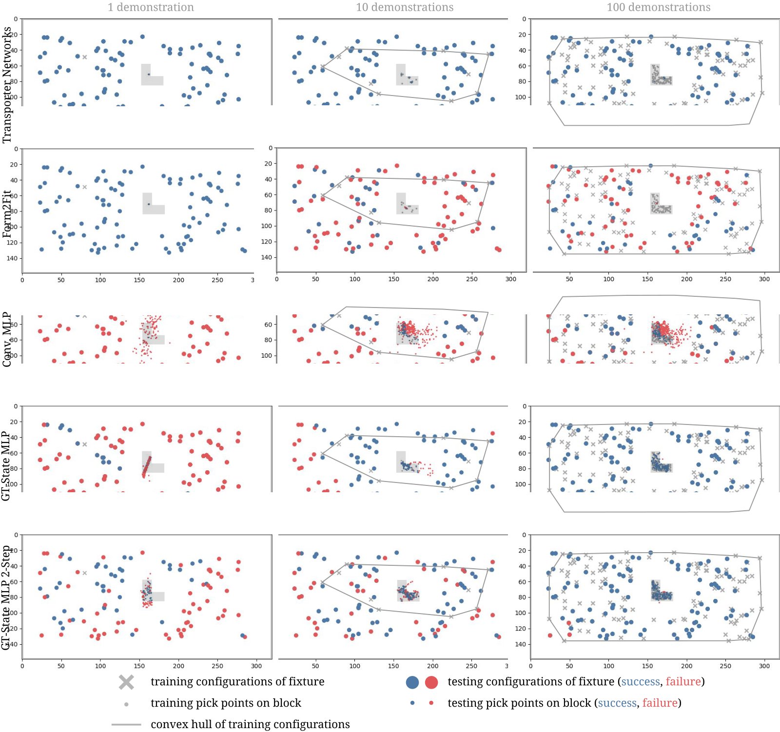
Figure 9: Depictions of the generalization ability of different models on the simplified translation-only block-insertion task. Each episode is visualized as a mark on the workspace (representing the pose of the fixture) – color-coded by task success (blue for success, red for failure). Environment configurations in the training set are shown in gray, and the convex hull of the training samples are drawn with a dotted line. Testing episodes inside the convex hell represent interpolation; those outside represent extrapolation. Plot inspired by [10].

图 9：不同模型在简化的仅平移积木插入任务上的泛化能力示意。每个回合在工作空间上可视化为一个标记（表示夹具位姿）——按任务成功着色（蓝为成功，红为失败）。训练集中的环境构型以灰色显示，训练样本的凸包用虚线画出。凸包内的测试回合代表插值；之外代表外推。绘图受 [10] 启发。

To gain a better qualitative understanding of the generalization abilities of Transporter Networks and the tested baseline models, we provide Fig. 9. Similar to the analysis in [10], this shows the spatial distribution of training configurations and successful/unsuccessful testing configurations–in this case, for translation-only block insertion with stochastic demonstrations. For each method we visualize its ability to interpolate and extrapolate from its training samples to handle new unseen poses of the target fixture.

为更好定性理解 Transporter Networks 与所测基线模型的泛化能力，我们给出图 9。与 [10] 中的分析类似，它展示训练构型以及成功/失败测试构型的空间分布——此处针对带随机示范的仅平移积木插入。对每种方法，我们可视化它从训练样本插值与外推、以处理目标夹具新未见位姿的能力。

As can be seen from these generalization plots, on this task Transporter Networks is capable of extrapolating to new testing episodes with just one demonstration. The dense deep feature transport operation enables the optimal placement of the block in the fixture to look similar under different picking and placing actions (exploiting translational equivariance of the task). This generalizes to new object configurations better than Conv MLP, which seems to only successfully interpolate around the majority of training episodes (often collapsing towards one mode of the training data).

从这些泛化图可见，在该任务上 Transporter Networks 仅用一条示范即可外推到新的测试回合。稠密深度特征搬运操作使积木在夹具中的最优放置，在不同抓取与放置动作下看起来相似（利用任务的平移等变性）。这比 Conv MLP 更好地泛化到新物体构型——后者似乎只在多数训练回合附近成功插值（常坍缩到训练数据的一个模式）。

Form2Fit is also capable of extrapolating from a single example, since both its picking and placing networks (also modeled by FCNs) are translationally equivariant – such that the block insertion task amounts to detecting the block and fixture under different translations. Once the number of demonstrations increase, however, the matching network is forced to learn pixel-wise descriptors that index multiple possible picking actions to multiple possible placing actions. In the setting with stochastic demonstrations, the positive-pair samples available for training the matching network are sparse and limited only to the pick-and-place action pairs from demonstrations – making it difficult to geometrically regularize the descriptors uniformly over the pixels on the surface of the block and the fixture. Minor mis-matches during testing can also lead to a slight misalignment of the block, which leads to poor placement and task failure. This suggests that Form2Fit’s matching network requires substantial training data to successful converge to a meaningful solution. The distribution of successful episodes with Form2Fit are also uniformly distributed over the workspace, which further confirms that its failures come largely from mismatching pick-and-place actions, rather than its inability to spatially interpolate or extrapolate.

Form2Fit 也能从单个例子外推，因为其抓取与放置网络（也由 FCN 建模）都具有平移等变性——使积木插入任务等同于在不同平移下检测积木与夹具。然而一旦示范数量增加，匹配网络被迫学习把多种可能抓取动作索引到多种可能放置动作的逐像素描述子。在随机示范设定下，可用于训练匹配网络的正对样本稀疏，且仅限于示范中的抓取—放置动作对——难以在积木与夹具表面像素上均匀地几何正则描述子。测试时轻微错配也会导致积木轻微不对齐，进而放置不佳、任务失败。这表明 Form2Fit 的匹配网络需要大量训练数据才能成功收敛到有意义的解。Form2Fit 成功回合的分布在工作空间上也均匀分布，进一步确认其失败主要来自抓取—放置动作错配，而非无法空间插值或外推。

In the low data regime (with 10 demonstrations), GT-State MLP seems to overtrain to correlations that do not necessarily enable task success, e.g., that picking locations are conditioned on the location of the target fixture (see distribution of failed pick locations and fixture locations). By dividing GT-State MLP into two steps – one for picking and one for placing, we see less issues with incorrect correlations. However, the inability to extrapolate too far beyond the distribution of training data still remains (e.g., see failure testing configurations of fixture for GT-State MLP 2-Step with 100 demonstrations, which also caused an incorrect pick point prediction).

在低数据体制（10 条示范）下，GT-State MLP 似乎过拟合到不一定能带来任务成功的相关，例如抓取位置以目标夹具位置为条件（见失败抓取位置与夹具位置的分布）。把 GT-State MLP 分成两步——一步抓取、一步放置后，错误相关问题变少。但无法外推到远超训练数据分布之外的问题仍然存在（例如见 GT-State MLP 2-Step 在 100 条示范下失败的夹具测试构型，它也导致了错误的抓取点预测）。

6.11 Ablation Studies

6.11 消融研究

Tab. 6 also reports the performance of various ablations of Transporter Networks:

表 6 还报告了 Transporter Networks 多种消融的表现：

No-Transport uses two FCNs: one to predict a picking heatmap, another to predict placing heatmaps (one per discretized rotation). The transport model is not used here, hence there is no pick-conditioned placing. For simpler tasks, such as place-red-in-green, this could suffice if the picking model predicts higher values on red pixels, and the placing model predicts higher values on green pixels. Or, for block-insertion, if the picking model detects the same location on the block, and the placing model detects the same corresponding location and orientation in the fixture. However, it is much more challenging to execute tasks that require additional visual reasoning, such as aligning unseen box corners. For palletizing and packing boxes, the learned policies are generally capable of placing a few of the boxes into the target zones, but fail to align them to each other tightly to achieve higher completion scores above 55%.

No-Transport 使用两个 FCN：一个预测抓取热图，另一个预测放置热图（每个离散旋转一张）。此处不使用搬运模型，因而没有以抓取为条件的放置。对更简单任务如 place-red-in-green，若抓取模型在红色像素上预测更高值、放置模型在绿色像素上预测更高值，这或许足够。或者对 block-insertion，若抓取模型检测到积木上同一位置，放置模型检测到夹具中对应同一位置与朝向。但对需要对齐未见盒子角等额外视觉推理的任务，挑战大得多。对码垛与装箱，学到的策略通常能把少数纸箱放入目标区，但无法把它们彼此紧密对齐以达到高于 55% 的完成分数。

Per-Pixel-CE-Loss is a variant of the Transporter Network, where the cross-entropy loss over the entire image (representing a single probability distribution) is replaced with per-pixel cross-entropy, where each pixel represents its own probability distribution. During training, for every demonstration pick-and-place: the picking and placing pixels unraveled from the data are chosen as positive samples for the models respectively, while a fixed number of 100 random negative pixels are sampled from everywhere else. In general, our experiments suggest that the model i) takes more training iterations to converge, and ii) requires more hyper-parameter tuning to balance the ratio of positives to negatives to regularize the loss over time.

Per-Pixel-CE-Loss 是 Transporter Network 的变体，把整幅图像上的交叉熵损失（表示单个概率分布）替换为逐像素交叉熵，每个像素表示自己的概率分布。训练时，对每次示范抓取放置：从数据展开的抓取与放置像素分别选为正样本，同时从其他所有地方采样固定数量 100 个随机负像素。总体而言，实验表明该模型 i）需要更多训练迭代才能收敛，ii）需要更多超参调优以平衡正负比例，从而随时间正则损失。

	block-insertion	place-red-in-green	towers-of-hanoi	align-box-corner	stack-block-pyramid
Method	1	10	100	1000	1	10	100	1000	1	10	100	1000	1	10	100	1000	1	10	100	1000
Per-Pixel-CE-Loss	89.0	88.0	91.0	90.0	87.5	100	100	100	29.6	57.0	57.9	64.6	46.0	65.0	73.0	77.0	23.0	28.0	33.7	36.0
No-Transport	5.0	8.0	6.0	8.0	81.5	95.7	100	100	2.1	3.6	4.7	3.3	9.0	7.0	11.0	15.0	8.0	13.2	16.0	25.8
	palletizing-boxes	assembling-kits	packing-boxes	manipulating-rope	sweeping-piles
	1	10	100	1000	1	10	100	1000	1	10	100	1000	1	10	100	1000	1	10	100	1000
Per-Pixel-CE-Loss	40.3	41.5	39.1	42.7	12.8	48.0	50.0	52.6	44.8	58.1	58.9	68.1	4.9	29.7	28.8	38.9	30.3	29.9	37.5	39.6
No-Transport	44.3	50.4	53.6	54.1	0.6	4.0	1.8	2.8	11.3	40.1	42.3	53.5	33.5	35.3	38.8	40.0	13.7	18.8	28.8	38.1

Table 6: Ablative comparisons. Task success rate (mean %) vs. # of demonstration episodes (1, 10, 100, or 1000) used in training.

	block-insertion	place-red-in-green	towers-of-hanoi	align-box-corner	stack-block-pyramid
方法	1	10	100	1000	1	10	100	1000	1	10	100	1000	1	10	100	1000	1	10	100	1000
Per-Pixel-CE-Loss	89.0	88.0	91.0	90.0	87.5	100	100	100	29.6	57.0	57.9	64.6	46.0	65.0	73.0	77.0	23.0	28.0	33.7	36.0
No-Transport	5.0	8.0	6.0	8.0	81.5	95.7	100	100	2.1	3.6	4.7	3.3	9.0	7.0	11.0	15.0	8.0	13.2	16.0	25.8
	palletizing-boxes	assembling-kits	packing-boxes	manipulating-rope	sweeping-piles
	1	10	100	1000	1	10	100	1000	1	10	100	1000	1	10	100	1000	1	10	100	1000
Per-Pixel-CE-Loss	40.3	41.5	39.1	42.7	12.8	48.0	50.0	52.6	44.8	58.1	58.9	68.1	4.9	29.7	28.8	38.9	30.3	29.9	37.5	39.6
No-Transport	44.3	50.4	53.6	54.1	0.6	4.0	1.8	2.8	11.3	40.1	42.3	53.5	33.5	35.3	38.8	40.0	13.7	18.8	28.8	38.1

表 6：消融对照。 任务成功率（平均 %）相对训练所用示范回合数（1、10、100 或 1000）。

6.12 Training Convergence

6.12 训练收敛

We train Transporter Networks with Adam [53], using fixed learning rates of $10^{-5}$. Our models are trained from scratch (i.e., random initialization) in Tensorflow. On the right, we show an example convergence plot over training from 100 demonstrations of manipulating rope. Compared with image-based baselines, Transporter Networks generally converge faster – within a few thousand training iterations, i.e., one or two hours of wall-clock time.

我们用 Adam [53] 训练 Transporter Networks，固定学习率 $10^{-5}$。模型在 Tensorflow 中从零（即随机初始化）训练。右侧展示从 100 条操纵绳索示范训练的收敛曲线例子。与基于图像的基线相比，Transporter Networks 通常收敛更快——在几千次训练迭代内，即一到两小时墙钟时间。

6.13 Visualizing Transporter Network Predictions

6.13 可视化 Transporter Network 预测

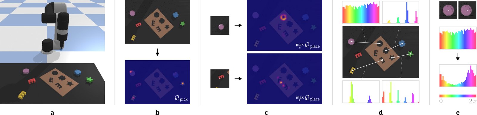
Figure 10: Visualizing Transporter Network Predictions. For the kit assembly task (a), Transporter Network picking predictions show 3 dominant modes on 3 different objects (b) which are not necessarily centered on the object (which may reflect biases learned from the distribution of training data). If a pick is off-center e.g., on the circle block, (c, top), the Transporter Network correctly makes placing predictions along the edges of the target placement location – which is visualized as a ring on $\mathcal{Q}_{\textrm{place}}$ maxed over rotations. If a pick is on the corner of the unseen E-shaped object (c, bottom), then two dominant modes lie on the correct corresponding locations of their target placements – but also with false positive modes from geometric symmetries in the letter E. We also show modes of predicted placing values over rotations for pick-and-place locations centered on the object and fixture, which appear uniform for circle, 4 modes for the cross shape, 5 modes for star shape, 2 modes for the unseen E-shaped block (dominant one being correct). We also visualize how the predicted placing values over rotations change from uniform, to unimodal, when shifting one pixel to the right from the center of the circle.

图 10：可视化 Transporter Network 预测。 对套件组装任务 (a)，Transporter Network 的抓取预测在 3 个不同物体上显示 3 个主导模式 (b)，不一定居中于物体（可能反映从训练数据分布学到的偏置）。若抓取偏离中心，例如在圆形积木上 (c，上)，Transporter Network 正确地沿目标放置位置边缘做放置预测——可视化为在旋转上取最大后的 $\mathcal{Q}_{\textrm{place}}$ 上的环。若抓取在未见 E 形物体的角上 (c，下)，则两个主导模式落在其目标放置的正确对应位置——但也有来自字母 E 几何对称性的假阳性模式。我们还展示以物体与夹具为中心的抓取放置位置上、放置值随旋转的预测模式：圆形近似均匀，十字形 4 个模式，星形 5 个模式，未见 E 形积木 2 个模式（主导者为正确）。我们还可视化：从圆形中心向右移一个像素时，放置值随旋转的预测如何从均匀变为单峰。

Fig. 10 visualizes Transporter Network dense pixel-wise predictions of $\mathcal{Q}_{\textrm{pick}}$ and $\mathcal{Q}_{\textrm{place}}$ for the kit assembly task (trained with 1,000 demonstrations), and how the predicted modes change with respect to the locations of objects, their shapes, and conditioned picks. These visualizations show that due to rotation and translation equivariance, our method can quickly learn modes that reflect symmetries in the data.

图 10 可视化 Transporter Network 对套件组装任务（用 1,000 条示范训练）的 $\mathcal{Q}_{\textrm{pick}}$ 与 $\mathcal{Q}_{\textrm{place}}$ 稠密逐像素预测，以及预测模式如何随物体位置、形状与条件抓取变化。这些可视化表明，由于旋转与平移等变性，我们的方法能快速学习反映数据对称性的模式。

These visualizations also show an interesting failure mode, in which predicted placements of the unseen E-shaped object returns several 180 degree flipped false positives (see Fig. 10c). This is because the learned features from this task rely strongly on local geometry. Since the E shape is a new unseen object, a flipped E looks similar enough to return a false positive signal there (though not enough to be the top mode).

这些可视化也显示一个有趣的失败模式：对未见 E 形物体的预测放置返回若干 180 度翻转的假阳性（见图 10c）。这是因为该任务学到的特征强烈依赖局部几何。由于 E 形是新的未见物体，翻转的 E 看起来足够相似以至在那里返回假阳性信号（尽管不足以成为最高模式）。

6.14 Real-World Experiments Details

6.14 真实世界实验细节

To demonstrate the real-world performance of Transporter Networks, we apply our approach to two challenging real-world tasks: assembling kits of mouthwash bottles with pick and place, and sweeping piles of small Go pieces with pushing. These tasks are shown in Fig. 11.

为展示 Transporter Networks 的真实世界表现，我们将方法应用于两项有挑战的真实任务：用抓取放置组装漱口水瓶套件，以及用推动清扫小围棋子堆。这些任务见图 11。

For kit assembly, we sequentially pick 5 small mouthwash bottles from a “bin” of identically shaped items and place each into a “kit” with 5 corresponding indentations for placement. This is a challenging task due to the multi-modality and ambiguity of the pick location (many identical items in the bin to pick from), as well as the tight millimeter tolerances of the destination kit. It is designed to mimic a production robotic task of placing items into a blister pack for consumer packaging. Kit assembly and disassembly are treated as separate tasks – both use the same Transporter Network architecture with autonomous switching between the two tasks at inference time. As shown in Table 5, our model achieves 98.9% on kit assembly, trained with 8,141 pick and place actions recorded from human demonstrations. Picking success and disassembly success are both above 99%.

对套件组装，我们依次从装有相同形状物品的「料箱」中抓取 5 个小漱口水瓶，并各自放入带 5 个对应凹槽的「套件」。该任务具有挑战性，因为抓取位置多峰且模糊（料箱中有许多相同物品可选），且目标套件公差紧到毫米级。它设计为模拟把物品放入泡罩包装的产线机器人任务。套件组装与拆卸视为独立任务——二者使用相同 Transporter Network 结构，推理时自主在两任务间切换。如表 5 所示，我们的模型在套件组装上达到 98.9%，用从人类示范记录的 8,141 次抓取放置动作训练。抓取成功与拆卸成功均高于 99%。

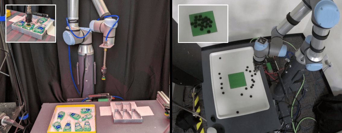
Figure 11: Real-world tasks. Left: assembling kits of mouthwash bottles, right: pushing piles of small Go pieces.

图 11：真实世界任务。 左： 组装漱口水瓶套件，右： 推动小围棋子堆。

For sweeping, we sequentially push piles of small Go pieces into a target goal zone, marked with green tape. Upon completion of the task, the robot autonomously resets with a scripted scrambling motion. This task is challenging as it tests the capacity of the model to sequence actions using closed-loop visual feedback, and to do it efficiently. As shown in Table 5, our model achieves 98.3% on this task, trained with 6,759 pushing actions recorded from human demonstrations. The average number of sweeps needed to complete the task is 20 $\pm$ 2.5 sweeps, with the fastest run being 16 sweeps and the slowest 25. For reference, the average for human teleoperation is 18.1 sweeps.

对清扫，我们依次把小围棋子堆推入用绿胶带标出的目标区。任务完成后，机器人用脚本化搅乱动作自主复位。该任务具有挑战性，因为它检验模型用闭环视觉反馈对动作排序、并高效完成的能力。如表 5 所示，我们的模型在该任务上达到 98.3%，用从人类示范记录的 6,759 次推动动作训练。完成任务所需平均清扫次数为 20 $\pm$ 2.5 次，最快 16 次、最慢 25 次。作为参考，人类遥操作平均为 18.1 次。

To train our system for both tasks, we use human demonstration data captured by a remote teleoperation interface. The sub-optimal, biased and noisy distribution of human demonstrations presents a further challenge for robotic policy learning. In addition, 13 teleoperators of varying skill and performance level provide training data, which further increases the variance of ground-truth actions that we train from and subsequently increases the difficulty of the learning task.

为训练两个任务的系统，我们使用远程遥操作界面采集的人类示范数据。人类示范次优、有偏且含噪的分布，给机器人策略学习带来进一步挑战。此外，13 名技能与表现水平各异的遥操作员提供训练数据，进一步提高我们训练所依据的真实动作方差，从而增加学习任务难度。

Hardware Setup

硬件设置

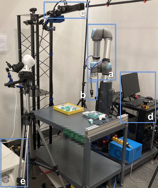
Figure 12: Hardware setup. a) UR5e Robot, b) Piab suction cup, c) Photoneo camera, d) Linux PC, and e) air compressor and vacuum generator.

图 12：硬件设置。 a) UR5e 机器人，b) Piab 吸盘，c) Photoneo 相机，d) Linux PC，以及 e) 空气压缩机与真空发生器。

The hardware setup for kit assembly is shown in Fig 12. Our experiments make use of 2 Universal Robots UR5 workstations (one for kit assembly and one for sweeping), each with an industrial Linux PC, vacuum system, Piab suction cup or brush end-effector, and depth camera (statically mounted above the workstation). To test the robustness of our method to diverse data sources, we use high quality depth camera observations from a Photoneo PhoXi Model M for kit assembly, and those from low cost consumer-grade Azure Kinect for sweeping. The Photoneo camera supplies depth (with 0.1mm rated depth precision) and a greyscale IR image, both at $1032\times 772$ resolution. The Kinect camera supplies depth as well as a color RGB image at $1280\times 720$ resolution.

套件组装的硬件设置见图 12。实验使用 2 台 Universal Robots UR5 工作站（一台用于套件组装，一台用于清扫），各配工业 Linux PC、真空系统、Piab 吸盘或刷子末端，以及深度相机（静态安装在工作站上方）。为测试方法对不同数据源的稳健性，套件组装使用 Photoneo PhoXi Model M 的高质量深度相机观测，清扫使用低成本消费级 Azure Kinect。Photoneo 相机提供深度（额定深度精度 0.1 mm）与灰度 IR 图像，分辨率均为 $1032\times 772$。Kinect 相机提供深度以及 $1280\times 720$ 分辨率的彩色 RGB 图像。

To calibrate the camera within the robot coordinate frame we use a two step procedure. Firstly, the intrinsics of the camera are calibrated by capturing multiple images of a large flat QR-Code panel in varying orientations, and we use OpenCV to calculate the camera intrinsics. Secondly, to calibrate extrinsics we attach QR code tags to the UR5 wrist joint and we capture multiple images of the robot in random end-effector poses. These images are then used to solve for the position of the robot base as well as the offset of the QR Tag to its respective joint with a stochastic optimization procedure.

为在机器人坐标系中标定相机，我们采用两步流程。首先，通过在不同朝向下拍摄大块平面二维码面板的多张图像标定相机内参，并用 OpenCV 计算内参。其次，为标定外参，我们在 UR5 腕关节贴上二维码标签，并在随机末端位姿下拍摄机器人多张图像。随后用这些图像，经随机优化流程求解机器人基座位姿以及二维码标签相对其关节的偏移。

A Linux system embedded with the robot gathers robot and camera data and forwards it to the teleoperator over the internet. Any commands passed to the robots are queued up to be processed one-by one. All data is logged in real-time via network to a cloud storage database for model training and evaluation.

嵌入机器人的 Linux 系统采集机器人与相机数据，并经互联网转发给遥操作员。传给机器人的任何命令排队逐一处理。所有数据经网络实时记入云存储数据库，用于模型训练与评估。

Data Collection

数据采集

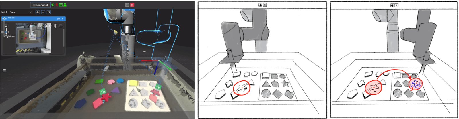
Figure 13: Data Collection UI. Left: Unity-based UI. Middle: The operator selects the area where the object is to be picked up. Right: The operator can adjust the placement of the object and rotate it. The depth image around the pick-up point is overlaid and helps the operator align the placement.

图 13：数据采集界面。 左： 基于 Unity 的界面。中： 操作员选择物体被抓取的区域。右： 操作员可调整物体放置并旋转。抓取点周围的深度图像叠加显示，帮助操作员对齐放置。

We designed a 2D User-Interface (UI) scripted in Unity [46] in order to control the robot workstations remotely. An overview of this UI is shown in Fig 13. Features of this UI include: configuration of the robot workcell, movement and actuation of the suction end-effector, configuration of parameterized action trajectories, calibration of the robot and control of the robot using the same action parameterization used to train our model.

我们设计了用 Unity [46] 脚本编写的二维用户界面（UI），以便远程控制机器人工作站。该界面概览见图 13。功能包括：配置机器人工作单元、吸盘末端的运动与驱动、配置参数化动作轨迹、标定机器人，以及用与训练模型相同的动作参数化控制机器人。

A standard teleoperation session is as follows. The operator views a 3D rendering of the workstation depth data. The synthetic camera view can be rotated and translated using mouse movements as desired by the operator. The operator determines with mouse clicks which object to pick by selecting the intended pick-up point on the rendered depth geometry. A region of the point cloud around the pick location is then “attached” to the mouse cursor, where it is rendered transparent and overlaid on the existing depth (illustrated in Fig 13). The operator is able to translate this geometry with movements of the mouse and the single rotational degree of freedom is controlled by the mouse wheel. Once the operator moves the object into the desired location, an additional mouse click will select the 3DOF place location. This interface allows the operator to visualize the intended 3D configuration of the pick-and-place operation before the action is executed. The discrete teleoperator pick-and-place locations are then translated into dense robot trajectories using a Cartesian controller, checked for collisions and other safety constraints, and subsequently executed on-robot. The user then repeats this process until the task is complete.

标准遥操作会话如下。操作员查看工作站深度数据的三维渲染。可用鼠标按需旋转与平移合成相机视角。操作员用鼠标点击在渲染深度几何上选择预期抓取点，以决定抓哪个物体。随后抓取位置周围的点云区域「附着」到鼠标光标，以透明方式渲染并叠加在现有深度上（见图 13）。操作员可用鼠标移动平移该几何，单一旋转自由度由鼠标滚轮控制。一旦操作员把物体移到期望位置，再点一次鼠标即选定三维自由度放置位置。该界面使操作员能在动作执行前可视化抓取放置操作的预期三维构型。离散的遥操作抓取放置位置随后经笛卡尔控制器转为稠密机器人轨迹，检查碰撞与其他安全约束，再在机器人上执行。用户重复该过程直至任务完成。

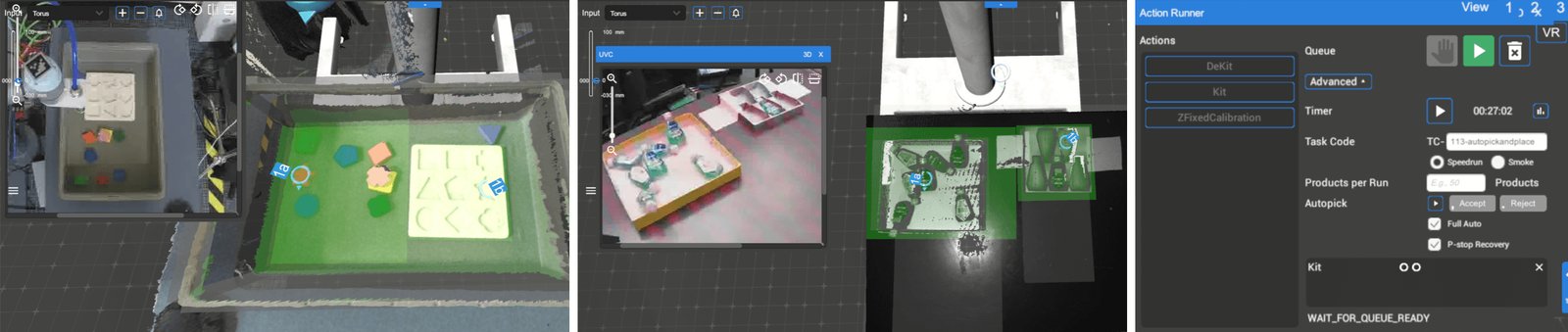
Figure 14: Autonomous Mode UI. User inputs the task to execute (by unique task code), and presses the play button to begin autonomous execution.

图 14：自主模式界面。 用户输入要执行的任务（用唯一任务代码），并按播放按钮开始自主执行。

Note that we use the same data pipeline and motion primitives when executing our Transporter Networks model as is used during human teleoperation; the human UI interaction is replaced with our inference results, and additional logic is added to switch between assembly and disassembly tasks. Autonomous mode is executing within the standard UI by first inputting the task to execute (by unique task code identifier), and pressing start. The UI for this (and visualization of inference results) is shown in Fig 14.

注意：执行 Transporter Networks 模型时，我们使用与人类遥操作相同的数据管线与运动基元；人类界面交互被我们的推理结果取代，并加入在组装与拆卸任务间切换的额外逻辑。自主模式在标准界面内执行：先输入要执行的任务（用唯一任务代码标识），再按开始。该界面（以及推理结果可视化）见图 14。

Using the above system we collected approximately 8,141 pick-and-place actions from 13 human operators in order to train the kit assembly model, an additional 2,300 actions for validation of model performance and hyper parameter tuning, and 6,759 pushing actions to train the sweeping model.

用上述系统，我们从 13 名人类操作员采集约 8,141 次抓取放置动作以训练套件组装模型，另有 2,300 次动作用于验证模型表现与超参调优，以及 6,759 次推动动作以训练清扫模型。

Success Detection

成功检测

For the on-robot evaluation in Section 4.2, we manually label robot actions for success or failure. However this process is time consuming and expensive. Additionally, our Transformer Network does not estimate when a multi-action kitting episode terminates (either successfully or unsuccessfully). So in order to perform fully-autonomous pick-and-place without manual success labelling, an automatic task-level success signal was implemented. We trained a ResNet50 classification model - pretrained on imagenet classification - to perform 3-way classification in order to detect full, empty or partial kits. We trained the classifier on 4848 training samples and evaluated on 128 validation set samples from a unique camera angle. Mean classification accuracy on the validation set was 96.9%. Upon completion of a pick-and-place attempt, classifier inference on the RGB image produces a success metric, which marks the successful completion of a Kitting (or emptying the kit) episode. This allows the fully autonomous mode of the system to alternate between tasks (kitting and emptying) upon completion.

对第 4.2 节的机上评估，我们人工标注机器人动作成功或失败。但该过程耗时且昂贵。此外，我们的 Transporter Network 并不估计多动作套件回合何时终止（无论成功或失败）。因此，为在不做人工成功标注的情况下实现完全自主抓取放置，实现了自动任务级成功信号。我们训练了一个在 ImageNet 分类上预训练的 ResNet50 分类模型，做三路分类以检测满、空或部分套件。分类器在 4848 个训练样本上训练，并在来自独特相机角度的 128 个验证集样本上评估。验证集平均分类准确率为 96.9%。抓取放置尝试完成后，对 RGB 图像做分类器推理产生成功度量，标记套件装填（或清空套件）回合成功完成。这使系统的完全自主模式能在完成后在任务（装填与清空）间交替。