Taskonomy: Disentangling Task Transfer Learning

Taskonomy：解耦任务迁移学习（Taskonomy: Disentangling Task Transfer Learning）

Amir R. Zamir Affiliation: Stanford University    Affiliation: University of California, Berkeley http://taskonomy.vision/    Alexander Sax † † thanks: Equal. Affiliation: Stanford University       William Shen    Leonidas Guibas Affiliation: Stanford University       Jitendra Malik Affiliation: University of California, Berkeley http://taskonomy.vision/    Silvio Savarese Affiliation: Stanford University

Amir R. Zamir（斯坦福大学；加州大学伯克利分校）　Alexander Sax*（斯坦福大学）　William Shen　Leonidas Guibas（斯坦福大学）　Jitendra Malik（加州大学伯克利分校）　Silvio Savarese（斯坦福大学）
*同等贡献。项目主页：http://taskonomy.vision/

Abstract

摘要

Do visual tasks have a relationship, or are they unrelated? For instance, could having surface normals simplify estimating the depth of an image? Intuition answers these questions positively, implying existence of a structure among visual tasks. Knowing this structure has notable values; it is the concept underlying transfer learning and provides a principled way for identifying redundancies across tasks, e.g., to seamlessly reuse supervision among related tasks or solve many tasks in one system without piling up the complexity.

视觉任务之间是否存在关系，还是彼此无关？例如，拥有表面法线（surface normals）是否会简化图像深度估计？直觉给出肯定答案，这意味着视觉任务之间存在一种结构。弄清这一结构很有价值：它是迁移学习的概念基础，能提供用于更高效学习的原则性方式，还能对尚未充分研究的任务空间进行显式建模。

We proposes a fully computational approach for modeling the structure of space of visual tasks. This is done via finding (first and higher-order) transfer learning dependencies across a dictionary of twenty six 2D, 2.5D, 3D, and semantic tasks in a latent space. The product is a computational taxonomic map for task transfer learning. We study the consequences of this structure, e.g. nontrivial emerged relationships, and exploit them to reduce the demand for labeled data. For example, we show that the total number of labeled datapoints needed for solving a set of 10 tasks can be reduced by roughly $\frac{2}{3}$ (compared to training independently) while keeping the performance nearly the same. We provide a set of tools for computing and probing this taxonomical structure including a solver that users can employ to devise efficient supervision policies for their use cases.

我们提出一种完全基于计算的方法，对视觉任务空间的结构建模。做法是：在潜空间中，对由二十六个 2D、2.5D、3D 与语义任务组成的词典，找出（一阶与高阶）迁移学习依赖。产物是一张用于任务迁移学习的计算分类图谱。我们研究这张图谱的涌现结构，并用它给出数据高效的学习课程：在有限监督预算下，决定应优先学习哪些任务、应向哪些任务迁移，从而最大化对全部任务集合的表现。实验表明，该方法能显著降低对标注数据的需求。

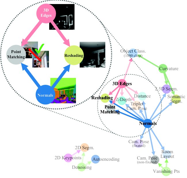
Figure 1: A sample task structure discovered by the computational task taxonomy (taskonomy). It found that, for instance, by combining the learned features of a surface normal estimator and occlusion edge detector, good networks for reshading and point matching can be rapidly trained with little labeled data.

图 1：由计算任务分类学（taskonomy）发现的任务结构示例。例如，它发现：把表面法线估计器与遮挡边缘检测器学到的特征组合起来，只需很少标注数据，就能快速训练出效果良好的重着色（reshading）与点匹配网络。

1 Introduction

1 引言

Object recognition, depth estimation, edge detection, pose estimation, etc are examples of common vision tasks deemed useful and tackled by the research community. Some of them have rather clear relationships: we understand that surface normals and depth are related (one is a derivate of the other), or vanishing points in a room are useful for orientation. Other relationships are less clear: how keypoint detection and the shading in a room can, together, perform pose estimation.

对象识别、深度估计、边缘检测、姿态估计等是研究界认为有用并解决的常见视觉任务的例子。 其中一些具有相当清晰的关系：我们知道表面法线和深度是相关的（一个是另一个的导数），或者房间中的消失点对于定向很有用。 其他关系不太清楚：关键点检测和房间中的阴影如何一起执行姿势估计。

The field of computer vision has indeed gone far without explicitly using these relationships. We have made remarkable progress by developing advanced learning machinery (e.g. ConvNets) capable of finding complex mappings from $X$ to $Y$ when many pairs of $(x,y)$ s.t. $x\in X,y\in Y$ are given as training data. This is usually referred to as fully supervised learning and often leads to problems being solved in isolation. Siloing tasks makes training a new task or a comprehensive perception system a Sisyphean challenge, whereby each task needs to be learned individually from scratch. Doing so ignores their quantifiably useful relationships leading to a massive labeled data requirement.

在没有明确使用这些关系的情况下，计算机视觉领域确实已经走了很长一段路。 通过开发先进的学习机器（例如 ConvNet），我们取得了显着的进展，当许多对$(x,y)$s.t. 存在时，能够找到从$X$到$Y$的复杂映射。$x\in X,y\in Y$作为训练数据给出。 这通常被称为完全监督学习，并且通常会导致问题被孤立地解决。 孤立任务使得训练新任务或综合感知系统成为西西弗斯式的挑战，每个任务都需要从头开始单独学习。 这样做会忽略它们可量化的有用关系，从而导致大量标记数据的需求。

Alternatively, a model aware of the relationships among tasks demands less supervision, uses less computation, and behaves in more predictable ways. Incorporating such a structure is the first stepping stone towards developing provably efficient comprehensive/universal perception models [34, 4], i.e. ones that can solve a large set of tasks before becoming intractable in supervision or computation demands. However, this task space structure and its effects are still largely unknown. The relationships are non-trivial, and finding them is complicated by the fact that we have imperfect learning models and optimizers. In this paper, we attempt to shed light on this underlying structure and present a framework for mapping the space of visual tasks. Here what we mean by “structure” is a collection of computationally found relations specifying which tasks supply useful information to another, and by how much (see Fig. 1).

或者，了解任务之间关系的模型需要更少的监督，使用更少的计算，并且以更可预测的方式运行。 结合这样的结构是开发可证明有效的综合/通用感知模型的第一个垫脚石 [34, 4]，即可以在变得难以处理监督或计算需求之前解决大量任务的模型。 然而，这种任务空间结构及其影响仍然很大程度上未知。 这些关系并不简单，而且由于我们的学习模型和优化器不完善，找到它们也很复杂。 在本文中，我们试图阐明这一底层结构，并提出一个用于映射视觉任务空间的框架。 这里我们所说的“结构”是指通过计算发现的关系的集合，指定哪些任务向另一个任务提供有用信息以及提供多少信息（见图 1）。

We employ a fully computational approach for this purpose, with neural networks as the adopted computational function class. In a feedforward network, each layer successively forms more abstract representations of the input containing the information needed for mapping the input to the output. These representations, however, can transmit statistics useful for solving other outputs (tasks), presumably if the tasks are related in some form [83, 19, 58, 46]. This is the basis of our approach: we computes an affinity matrix among tasks based on whether the solution for one task can be sufficiently easily read out of the representation trained for another task. Such transfers are exhaustively sampled, and a Binary Integer Programming formulation extracts a globally efficient transfer policy from them. We show this model leads to solving tasks with far less data than learning them independently and the resulting structure holds on common datasets (ImageNet [78] and Places [104]).

为此，我们采用完全计算的方法，以神经网络作为采用的计算函数类。 在前馈网络中，每一层相继形成输入的更抽象表示，其中包含将输入映射到输出所需的信息。 然而，这些表示可以传输对解决其他输出（任务）有用的统计数据，假设这些任务以某种形式相关[83,19,58,46]。 这是我们方法的基础：我们根据一个任务的解决方案是否可以足够容易地从为另一任务训练的表示中读出来计算任务之间的亲和力矩阵。 此类传输经过详尽的采样，并且二进制整数规划公式从中提取了全局有效的传输策略。 我们证明，该模型可以用比独立学习少得多的数据来解决任务，并且所得结构适用于常见数据集（ImageNet [78] 和 Places [104]）。

Being fully computational and representation-based, the proposed approach avoids imposing prior (possibly incorrect) assumptions on the task space. This is crucial because the priors about task relations are often derived from either human intuition or analytical knowledge, while neural networks need not operate on the same principles [63, 33, 40, 45, 102, 88]. For instance, although we might expect depth to transfer to surface normals better (derivatives are easy), the opposite is found to be the better direction in a computational framework (i.e. suited neural networks better).

所提出的方法是完全计算和基于表示的，避免了对任务空间强加先前的（可能不正确的）假设。 这一点至关重要，因为任务关系的先验通常来自人类直觉或分析知识，而神经网络不需要按照相同的原理运行[63,33,40,45,102,88]。 例如，虽然我们可能期望深度更好地转移到表面法线（导数很容易），但发现相反的方向是计算框架中更好的方向（即更适合神经网络）。

An interactive taxonomy solver which uses our model to suggest data-efficient curricula, a live demo, dataset, and code are available at http://taskonomy.vision/.

交互式分类求解器使用我们的模型来建议数据高效的课程、现场演示、数据集和代码，请访问 http://taskonomy.vision/。

2 Related Work

2 相关工作

Assertions of existence of a structure among tasks date back to the early years of modern computer science, e.g. with Turing arguing for using learning elements [95, 98] rather than the final outcome or Jean Piaget’s works on developmental stages using previously learned stages as sources [74, 39, 38], and have extended to recent works [76, 73, 50, 18, 97, 61, 11, 66]. Here we make an attempt to actually find this structure. We acknowledge that this is related to a breadth of topics, e.g. compositional modeling [35, 10, 13, 23, 55, 92, 90], homomorphic cryptography [42], lifelong learning [93, 15, 85, 84], functional maps [71], certain aspects of Bayesian inference and Dirichlet processes [54, 91, 90, 89, 37, 39], few-shot learning [81, 25, 24, 70, 86], transfer learning [75, 84, 29, 64, 67, 59], un/semi/self-supervised learning [22, 8, 17, 103, 19, 83], which are studied across various fields [73, 94, 12]. We review the topics most pertinent to vision within the constraints of space:

任务之间存在结构的断言可以追溯到现代计算机科学的早期，例如 图灵主张使用学习元素[95, 98]，而不是最终结果，或者Jean Piaget关于发展阶段的著作使用先前学习的阶段作为来源[74,39,38]，并扩展到最近的著作[76,73,50,18,97,61,11,66]。 在这里我们尝试实际找到这个结构。 我们承认这涉及广泛的主题，例如 组合建模[35,10,13,23,55,92,90]，同态密码学[42]，终身学习[93,15,85,84]，功能图[71]，贝叶斯推理和狄利克雷过程的某些方面[54,91,90,89,37,39]，小样本学习[81， 25,24,70,86]，迁移学习[75,84,29,64,67,59]，非/半/自监督学习[22,8,17,103,19,83]，这些在各个领域都有研究[73,94,12]。 我们在空间限制内回顾与视觉最相关的主题：

Self-supervised learning methods leverage the inherent relationships between tasks to learn a desired expensive one (e.g. object detection) via a cheap surrogate (e.g. colorization) [68, 72, 17, 103, 100, 69]. Specifically, they use a manually-entered local part of the structure in the task space (as the surrogate task is manually defined). In contrast, our approach models this large space of tasks in a computational manner and can discover obscure relationships.

自监督学习方法利用任务之间的固有关系，通过廉价的替代项（例如着色）来学习所需的昂贵任务（例如对象检测）[68,72,17,103,100,69]。 具体来说，他们使用任务空间中手动输入的结构的本地部分（因为代理任务是手动定义的）。 相比之下，我们的方法以计算方式对如此大的任务空间进行建模，并且可以发现模糊的关系。

Unsupervised learning is concerned with the redundancies in the input domain and leveraging them for forming compact representations, which are usually agnostic to the downstream task [8, 49, 20, 9, 32, 77]. Our approach is not unsupervised by definition as it is not agnostic to the tasks. Instead, it models the space tasks belong to and in a way utilizes the functional redundancies among tasks.

无监督学习关注输入域中的冗余并利用它们形成紧凑的表示，这通常与下游任务无关[8,49,20,9,32,77]。 我们的方法并不是不受定义的监督，因为它对任务不是不可知的。 相反，它对任务所属的空间进行建模，并以某种方式利用任务之间的“功能”冗余。

Meta-learning generally seeks performing the learning at a level higher than where conventional learning occurs, e.g. as employed in reinforcement learning [21, 31, 28], optimization [2, 82, 48], or certain architectural mechanisms [27, 30, 87, 65]. The motivation behind meta learning has similarities to ours and our outcome can be seen as a computational meta-structure of the space of tasks.

元学习通常寻求比传统学习更高的水平进行学习，例如 如强化学习 [21,31,28]、优化 [2,82,48] 或某些架构机制 [27,30,87,65] 中所采用的。 元学习背后的动机与我们的相似，我们的结果可以被视为任务空间的计算元结构。

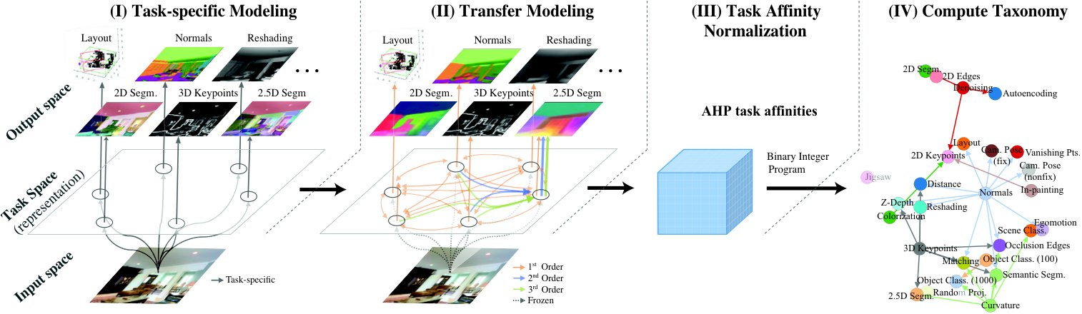
Figure 2: Computational modeling of task relations and creating the taxonomy. From left to right: I. Train task-specific networks. II. Train (first order and higher) transfer functions among tasks in a latent space. III. Get normalized transfer affinities using AHP (Analytic Hierarchy Process). IV. Find global transfer taxonomy using BIP (Binary Integer Program).

图 2：任务关系的计算建模和创建分类法。 从左到右：I. 训练特定任务网络。 二. 在潜在空间中的任务之间训练（一阶及更高阶）传递函数。 三． 使用 AHP（层次分析法）获得标准化的转移亲和力。 四． 使用 BIP（二进制整数程序）查找全局传输分类。

Multi-task learning targets developing systems that can provide multiple outputs for an input in one run [50, 18]. Multi-task learning has experienced recent progress and the reported advantages are another support for existence of a useful structure among tasks [93, 100, 50, 76, 73, 50, 18, 97, 61, 11, 66]. Unlike multi-task learning, we explicitly model the relations among tasks and extract a meta-structure. The large number of tasks we consider also makes developing one multi-task network for all infeasible.

多任务学习的目标是开发可以在一次运行中为输入提供多个输出的系统 [50, 18]。 多任务学习最近取得了进展，所报告的优点是任务之间存在有用结构的另一个支持[93,100,50,76,73,50,18,97,61,11,66]。 与多任务学习不同，我们明确地对任务之间的关系进行建模并提取元结构。 我们考虑的大量任务也使得为所有人开发一个多任务网络变得不可行。

Domain adaption seeks to render a function that is developed on a certain domain applicable to another [44, 99, 5, 80, 52, 26, 36]. It often addresses a shift in the input domain, e.g. webcam images to D-SLR [47], while the task is kept the same. In contrast, our framework is concerned with output (task) space, hence can be viewed as task/output adaptation. We also perform the adaptation in a larger space among many elements, rather than two or a few.

领域适应旨在呈现在某个领域开发的功能适用于另一个领域[44,99,5,80,52,26,36]。 它通常解决输入域中的转变，例如 网络摄像头图像传输到 D-SLR [47]，同时任务保持不变。 相比之下，我们的框架关注的是输出（任务）空间，因此可以被视为任务/输出适应。 我们还在更大的空间中对许多元素进行适应，而不是两个或几个元素。

In the context of our approach to modeling transfer learning across tasks:

在我们跨任务的迁移学习建模方法的背景下：

Learning Theoretic approaches may overlap with any of the above topics and usually focus on providing generalization guarantees. They vary in their approach: e.g. by modeling transferability with the transfer family required to map a hypothesis for one task onto a hypothesis for another [7], through information-based approaches [60], or through modeling inductive bias [6]. For these guarantees, learning theoretic approaches usually rely on intractable computations, or avoid such computations by restricting the model or task. Our method draws inspiration from theoretical approaches but eschews (for now) theoretical guarantees in order to use modern neural machinery.

学习理论方法可能与上述任何主题重叠，并且通常侧重于提供泛化保证。 他们的方法各不相同：例如 通过使用将一项任务的假设映射到另一项任务的假设所需的转移族来建模可转移性[7]，通过基于信息的方法[60]，或通过建模归纳偏差[6]。 为了这些保证，学习理论方法通常依赖于棘手的计算，或者通过限制模型或任务来避免此类计算。 我们的方法从理论方法中汲取灵感，但（目前）避开理论保证，以便使用现代神经机制。

3 Method

3 方法

We define the problem as follows: we want to maximize the collective performance on a set of tasks $\mathcal{T}=\{t_{1},...,t_{n}\}$, subject to the constraint that we have a limited supervision budget $\gamma$ (due to financial, computational, or time constraints). We define our supervision budget $\gamma$ to be the maximum allowable number of tasks that we are willing to train from scratch (i.e. source tasks). The task dictionary is defined as $\mathcal{V}$=$\mathcal{T}\cup\mathcal{S}$ where $\mathcal{T}$ is the set of tasks which we want solved (target), and $\mathcal{S}$ is the set of tasks that can be trained (source). Therefore, $\mathcal{T}-\mathcal{T}\cap\mathcal{S}$ are the tasks that we want solved but cannot train (“target-only”), $\mathcal{T}\cap\mathcal{S}$ are the tasks that we want solved but could play as source too, and $\mathcal{S}-\mathcal{T}\cap\mathcal{S}$ are the “source-only” tasks which we may not directly care about to solve (e.g. jigsaw puzzle) but can be optionally used if they increase the performance on $\mathcal{T}$.

问题定义如下：我们希望在任务集合 $\mathcal{T}=\{t_{1},...,t_{n}\}$ 上最大化整体表现，同时监督预算 $\gamma$ 有限（受资金、算力或时间约束）。我们将 $\gamma$ 定义为允许用完整标注训练的任务数上限。

The task taxonomy (taskonomy) is a computationally found directed hypergraph that captures the notion of task transferability over any given task dictionary. An edge between a group of source tasks and a target task represents a feasible transfer case and its weight is the prediction of its performance. We use these edges to estimate the globally optimal transfer policy to solve $\mathcal{T}$. Taxonomy produces a family of such graphs, parameterized by the available supervision budget, chosen tasks, transfer orders, and transfer functions’ expressiveness.

任务分类学（taskonomy）是一张用计算方式得到的有向超图，刻画给定任务词典上的任务可迁移性。从一组源任务指向目标任务的边表示可行的迁移情形，边权是对其表现的预测。我们用这些边估计最优迁移策略，从而在预算内最大化集体表现。

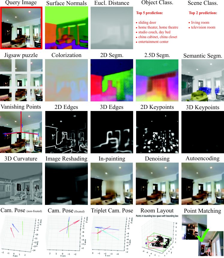
Figure 3: Task Dictionary. Outputs of 24 (of 26) task-specific networks for a query (top left). See results of applying frame-wise on a video here.

图 3：任务词典。 查询的 24 个（共 26 个）任务特定网络的输出（左上）。 请在此处查看在视频上应用逐帧的结果。

Taxonomy is built using a four step process depicted in Fig. 2. In stage I, a task-specific network for each task in $\mathcal{S}$ is trained. In stage II, all feasible transfers between sources and targets are trained. We include higher-order transfers which use multiple inputs task to transfer to one target. In stage III, the task affinities acquired from transfer function performances are normalized, and in stage IV, we synthesize a hypergraph which can predict the performance of any transfer policy and optimize for the optimal one.

分类学按图 2 所示四步构建。阶段 I：为 $\mathcal{S}$ 中每个任务训练任务专用网络。阶段 II：训练源与目标之间所有可行迁移（含使用多个输入任务的高阶迁移）。阶段 III：用 AHP 把迁移得到的亲和度归一化。阶段 IV：用 BIP 在预算约束下求解全局迁移策略。

A vision task is an abstraction read from a raw image. We denote a task $t$ more formally as a function $f_{t}$ which maps image $I$ to $f_{t}(I)$. Our dataset, $\mathcal{D}$, contains for each task $t$ a set of training pairs $(I,f_{t}(I))$, e.g. $(image,depth)$.

视觉任务是从原始图像中读取的抽象。 我们将任务$t$更正式地表示为函数$f_{t}$，它将图像$I$映射到$f_{t}(I)$。 我们的数据集$\mathcal{D}$包含每个任务$t$的一组训练对$(I,f_{t}(I))$，例如 XX数学7XX。

Task Dictionary: Our mapping of task space is done via (26) tasks included in the dictionary, so we ensure they cover common themes in computer vision (2D, 3D, semantics, etc) to the elucidate fine-grained structures of task space. See Fig. 3 for some of the tasks with detailed definition of each task provided in the supplementary material. We include tasks with various levels of abstraction, ranging from solvable by a simple kernel convolved over the image (e.g. edge detection) to tasks requiring basic understanding of scene geometry (e.g. vanishing points) and more abstract ones involving semantics (e.g. scene classification).

任务字典： 我们对任务空间的映射是通过字典中包含的 (26) 个任务完成的，因此我们确保它们涵盖计算机视觉中的常见主题（2D、3D、语义等），以阐明任务空间的细粒度结构。 有关一些任务，请参见图 3，补充材料中提供了每个任务的详细定义。 我们包括具有不同抽象级别的任务，从可通过图像上卷积的简单内核（例如边缘检测）来解决的任务，到需要对场景几何形状有基本了解的任务（例如消失点）以及涉及语义的更抽象的任务（例如场景分类）。

It is critical to note the task dictionary is meant to be a sampled set, not an exhaustive list, from a denser space of all conceivable visual tasks. Sampling gives us a tractable way to sparsely model a dense space, and the hypothesis is that (subject to a proper sampling) the derived model should generalize to out-of-dictionary tasks. The more regular / better sampled the space, the better the generalization. We evaluate this in Sec. 4.2 with supportive results. For evaluation of the robustness of results w.r.t the choice of dictionary, see the supplementary material.

值得注意的是，任务字典是一个“采样集，而不是详尽的列表”，来自所有可想象的视觉任务的密集空间。 采样为我们提供了一种对密集空间进行稀疏建模的易处理方法，并且假设（根据适当的采样）导出的模型应该推广到字典外的任务。 空间越规则/采样得越好，泛化效果就越好。 我们在第二节对此进行评估。 4.2 具有支持性结果。 要评估结果与词典选择的稳健性，请参阅补充材料。

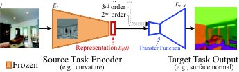
Figure 4: Transfer Function. A small readout function is trained to map representations of source task’s frozen encoder to target task’s labels. If order$>1$, transfer function receives representations from multiple sources.

图 4：传递函数。 训练一个小型读出函数，将源任务的冻结编码器的表示映射到目标任务的标签。 如果订购$>1$，传递函数会接收来自多个来源的表示。

Dataset: We need a dataset that has annotations for every task on every image. Training all of our tasks on exactly the same pixels eliminates the possibility that the observed transferabilities are affected by different input data peculiarities rather than only task intrinsics. There has not been such a dataset of scale made of real images, so we created a dataset of 4 million images of indoor scenes from about 600 buildings; every image has an annotation for every task. The images are registered on and aligned with building-wide meshes similar to [3, 101, 14] enabling us to programmatically compute the ground truth for many tasks without human labeling. For the tasks that still require labels (e.g. scene classes), we generate them using Knowledge Distillation [43] from known methods [104, 57, 56, 78]. See the supplementary material for full details of the process and a user study on the final quality of labels generated using Knowledge Distillation (showing $<7\%$ error).

数据集：我们需要一个包含每个图像上的每个任务的注释的数据集。 在完全相同的像素上训练我们的所有任务，消除了观察到的可传递性受到不同输入数据特性影响的可能性，而不仅仅是任务内在因素的影响。 目前还没有这样由真实图像组成的规模数据集，因此我们创建了约 600 座建筑物的 400 万张室内场景图像的数据集； 每个图像都有每个任务的注释。 这些图像在类似于 [3, 101, 14] 的建筑物范围内的网格上注册并对齐，使我们能够以编程方式计算许多任务的基本事实，而无需人工标记。 对于仍然需要标签的任务（例如场景类），我们使用知识蒸馏[43]从已知方法[104、57、56、78]生成它们。 有关该过程的完整详细信息以及有关使用知识蒸馏生成的标签的最终质量的用户研究（显示$<7\%$错误），请参阅补充材料。

3.1 Step I: Task-Specific Modeling

3.1 步骤 I：任务专用建模

We train a fully supervised task-specific network for each task in $\mathcal{S}$. Task-specific networks have an encoder-decoder architecture homogeneous across all tasks, where the encoder is large enough to extract powerful representations, and the decoder is large enough to achieve a good performance but is much smaller than the encoder.

我们为 $\mathcal{S}$ 中每个任务训练全监督的任务专用网络。各网络采用同构的编码器–解码器结构：编码器足够大以提取强表示，解码器足以达到良好表现，但远小于编码器。

3.2 Step II: Transfer Modeling

3.2 步骤 II：迁移建模

Given a source task $s$ and a target task $t$, where $s\in\mathcal{S}$ and $t\in\mathcal{T}$, a transfer network learns a small readout function for $t$ given a statistic computed for $s$ (see Fig 4). The statistic is the representation for image $I$ from the encoder of $s$: $E_{s}(I)$. The readout function ($D_{s\rightarrow t}$) is parameterized by $\theta_{s\rightarrow t}$ minimizing the loss $L_{t}$:

给定源任务 $s$ 与目标任务 $t$（$s\in\mathcal{S}$，$t\in\mathcal{T}$），迁移网络学习一个从小统计量到 $t$ 的读出函数（见图 4）。该统计量是源任务编码器对图像 $I$ 的表示：$E_{s}(I)$。读出函数 $D_{s\rightarrow t}$ 由浅层网络参数化。

$$D_{s\rightarrow t}\vcentcolon=\arg\min_{\theta}\mathbb{E}_{I\in\mathcal{D}}\Big[L_{t}\Big(D_{\theta}\big(E_{s}(I)\big),f_{t}(I)\Big)\Big], \tag{1}$$

where $f_{t}(I)$ is ground truth of $t$ for image $I$. $E_{s}(I)$ may or may not be sufficient for solving $t$ depending on the relation between $t$ and $s$ (examples in Fig. 5). Thus, the performance of $D_{s\rightarrow t}$ is a useful metric as task affinity. We train transfer functions for all feasible source-target combinations.

其中$f_{t}(I)$是图像$I$的$t$的基本事实。$E_{s}(I)$可能足以也可能不足以求解 $t$，具体取决于$t$和$s$之间的关系（图 5 中的示例）。 因此，$D_{s\rightarrow t}$ 的性能作为任务关联性是一个有用的指标。 我们为所有可行的源-目标组合训练传递函数。

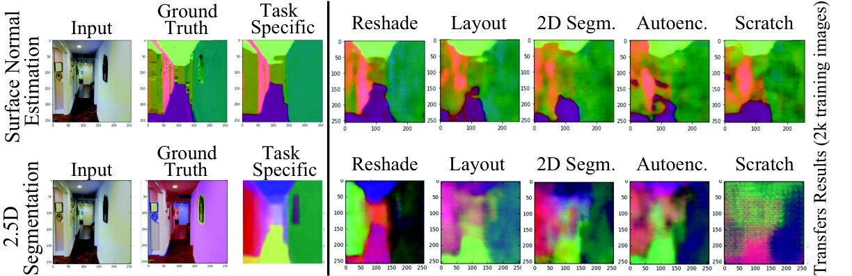
Figure 5: Transfer results to normals (upper) and 2.5D Segmentation (lower) from 5 different source tasks. The spread in transferability among different sources is apparent, with reshading among top-performing ones in this case. Task-specific networks were trained on 60x more data. “Scratch” was trained from scratch without transfer learning.

图 5：将结果从 5 个不同的源任务传输到法线（上）和 2.5D 分割（下）。 不同来源之间的可转移性分布很明显，在这种情况下，表现最好的来源会重新着色。 特定任务网络接受了 60 倍以上的数据训练。 “Scratch”是从头开始训练的，没有迁移学习。

Accessibility: For a transfer to be successful, the latent representation of the source should both be inclusive of sufficient information for solving the target and have the information accessible, i.e. easily extractable (otherwise, the raw image or its compression based representations would be optimal). Thus, it is crucial for us to adopt a low-capacity (small) architecture as transfer function trained with a small amount of data, in order to measure transferability conditioned on being highly accessible. We use a shallow fully convolutional network and train it with little data (8x to 120x less than task-specific networks).

可访问性：为了成功传输，源的潜在表示应该“包含”足够的信息来解决目标，并且具有“可访问”的信息，即易于提取（否则，原始图像或其基于压缩的表示将是最佳的）。 因此，对于我们来说，采用低容量（小）架构作为用少量数据训练的传递函数至关重要，以便测量以高度可访问为条件的可传递性。 我们使用浅层全卷积网络并用很少的数据对其进行训练（比特定任务网络少 8 倍到 120 倍）。

Higher-Order Transfers: Multiple source tasks can contain complementary information for solving a target task (see examples in Fig 6). We include higher-order transfers which are the same as first order but receive multiple representations in the input. Thus, our transfers are functions $D:\wp(\mathcal{S})\rightarrow\mathcal{T}$, where $\wp$ is the powerset operator.

高阶传输： 多个源任务可以包含用于解决目标任务的补充信息（参见图 6 中的示例）。 我们包括与一阶相同的高阶传输，但在输入中接收多个表示。 因此，我们的传输是函数$D:\wp(\mathcal{S})\rightarrow\mathcal{T}$，其中$\wp$是幂集运算符。

As there is a combinatorial explosion in the number of feasible higher-order transfers ($|\mathcal{T}|\times{|\mathcal{S}|\choose k}$ for $k^{th}$ order), we employ a sampling procedure with the goal of filtering out higher-order transfers that are less likely to yield good results, without training them. We use a beam search: for transfers of order $k\leq 5$ to a target, we select its 5 best sources (according to $1^{st}$ order performances) and include all of their order-$k$ combination. For $k\geq 5$, we use a beam of size 1 and compute the transfer from the top $k$ sources.

由于可行的高阶传输数量出现组合爆炸（$|\mathcal{T}|\times{|\mathcal{S}|\choose k}$ 代表$k^{th}$阶），我们采用采样程序，其目标是过滤掉不太可能产生良好结果的高阶传输，而不对其进行训练。 我们使用波束搜索：为了将$k\leq 5$阶转移到目标，我们选择其 5 个最佳源（根据$1^{st}$阶性能）并包括它们的所有阶 -$k$组合。 对于$k\geq 5$，我们使用大小为 1 的光束并计算来自顶部$k$源的传输。

Transitive Transfers: We examined if transitive task transfers ($s\rightarrow t_{1}\rightarrow t_{2}$) could improve the performance over their direct counterpart ($a\rightarrow t_{2}$), but found that the two had equal performance in almost all cases in both high-data and low-data scenarios. The experiment is provided in the supplementary material. Therefore, we need not consider the cases where branching would be more than one level deep when searching for the optimal transfer path.

传递性传输：我们检查了传递性任务传输 ($s\rightarrow t_{1}\rightarrow t_{2}$) 是否可以比直接对应的任务传输 ($a\rightarrow t_{2}$) 提高性能，但发现两者在高数据和低数据场景中几乎所有情况下都具有相同的性能。 该实验在补充材料中提供。 因此，在搜索最佳传输路径时，我们不需要考虑分支深度超过一级的情况。

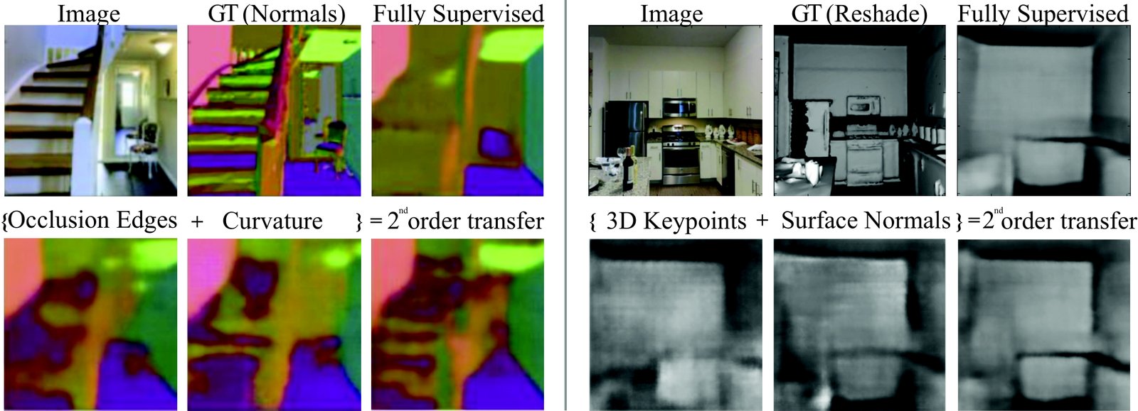
Figure 6: Higher-Order Transfers. Representations can contain complementary information. E.g. by transferring simultaneously from 3D Edges and Curvature individual stairs were brought out. See our publicly available interactive transfer visualization page for more examples.

图 6：高阶传输。 表示可以包含补充信息。 例如。 通过同时从 3D Edges 和 Curvature 传输，单独的楼梯被带出来。 请参阅我们公开的交互式传输可视化页面以获取更多示例。

3.3 Step III: Ordinal Normalization using Analytic Hierarchy Process (AHP)

3.3 步骤 III：用层次分析法（AHP）做序数归一化

We want to have an affinity matrix of transferabilities across tasks. Aggregating the raw losses/evaluations $L_{s\rightarrow t}$ from transfer functions into a matrix is obviously problematic as they have vastly different scales and live in different spaces (see Fig. 7-left). Hence, a proper normalization is needed. A naive solution would be to linearly rescale each row of the matrix to the range $[0,1]$. This approach fails when the actual output quality increases at different speeds w.r.t. the loss. As the loss-quality curve is generally unknown, such approaches to normalization are ineffective.

我们希望有一个跨任务可转移性的亲和力矩阵。 将传递函数中的原始损失/评估$L_{s\rightarrow t}$聚合到矩阵中显然是有问题的，因为它们具有截然不同的尺度并且存在于不同的空间中（见图 7-左）。 因此，需要适当的标准化。 一个简单的解决方案是将矩阵的每一行线性重新缩放到范围$[0,1]$。 当实际输出质量以不同的速度增加时，这种方法就会失败。 损失。 由于损失质量曲线通常是未知的，因此这种标准化方法是无效的。

Instead, we use an ordinal approach in which the output quality and loss are only assumed to change monotonically. For each $t$, we construct $W_{t}$ a pairwise tournament matrix between all feasible sources for transferring to $t$. The element at $(i,j)$ is the percentage of images in a held-out test set, $\mathcal{D}_{test}$, on which $s_{i}$ transfered to $t$ better than $s_{j}$ did (i.e. $D_{s_{i}\rightarrow t}(I)>D_{s_{j}\rightarrow t}(I)$).

相反，我们使用“序数”方法，其中仅假设输出质量和损失单调变化。 对于每个$t$，我们在所有可行源之间构造$W_{t}$成对的锦标赛矩阵，以便转移到$t$。$(i,j)$中的元素是保留测试集$\mathcal{D}_{test}$中图像的百分比，其中$s_{i}$比$s_{j}$更好地转移到 $t$（即$D_{s_{i}\rightarrow t}(I)>D_{s_{j}\rightarrow t}(I)$）。

We clip this intermediate pairwise matrix $W_{t}$ to be in $[0.001,0.999]$ as a form of Laplace smoothing. Then we divide $W^{\prime}_{t}=W_{t}/W_{t}^{T}$ so that the matrix shows how many times better $s_{i}$ is compared to $s_{j}$. The final tournament ratio matrix is positive reciprocal with each element $w^{\prime}_{i,j}$ of $W^{\prime}_{t}$:

我们将这个中间成对矩阵$W_{t}$剪裁为$[0.001,0.999]$作为拉普拉斯平滑的一种形式。 然后我们除以$W^{\prime}_{t}=W_{t}/W_{t}^{T}$，以便矩阵显示$s_{i}$比$s_{j}$好多少倍。 最终的锦标赛比率矩阵与$W^{\prime}_{t}$的每个元素$w^{\prime}_{i,j}$呈正倒数：

$$w^{\prime}_{i,j}=\frac{\mathop{\mathbb{E}}_{I\in\mathcal{D_{\textit{test}}}}[D_{s_{i}\rightarrow t}(I)>D_{s_{j}\rightarrow t}(I)]}{\mathop{\mathbb{E}}_{I\in\mathcal{D_{\textit{test}}}}[D_{s_{i}\rightarrow t}(I)<D_{s_{j}\rightarrow t}(I)]}. \tag{2}$$

We quantify the final transferability of $s_{i}$ to $t$ as the corresponding ($i^{th}$) component of the principal eigenvector of $W^{\prime}_{t}$ (normalized to sum to 1). The elements of the principal eigenvector are a measure of centrality, and are proportional to the amount of time that an infinite-length random walk on $W^{\prime}_{t}$ will spend at any given source [62]. We stack the principal eigenvectors of $W^{\prime}_{t}$ for all $t\in\mathcal{T}$, to get an affinity matrix $P$ (‘p’ for performance)—see Fig. 7, right.

我们将$s_{i}$到$t$的最终可转移性量化为$W^{\prime}_{t}$主特征向量的相应 ($i^{th}$) 分量（归一化为总和为 1）。 主特征向量的元素是中心性的度量，并且与$W^{\prime}_{t}$上的无限长度随机游走在任何给定源处花费的时间量成正比 [62]。 我们将所有$t\in\mathcal{T}$的$W^{\prime}_{t}$的主特征向量叠加，得到亲和力矩阵 $P$（‘p’代表性能）——见图 7，右图。

This approach is derived from Analytic Hierarchy Process [79], a method widely used in operations research to create a total order based on multiple pairwise comparisons.

这种方法源自层次分析法[79]，这是一种在运筹学中广泛使用的方法，用于基于多个成对比较创建总顺序。

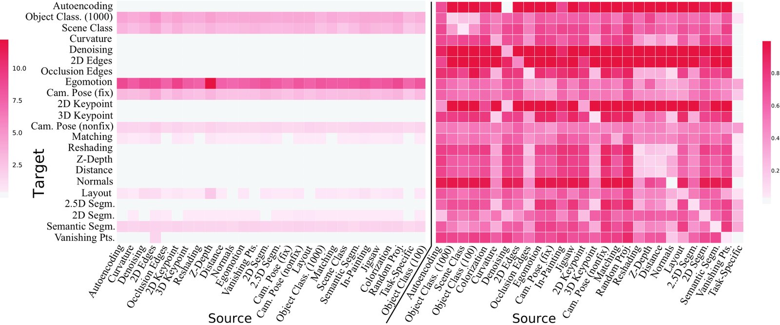
Figure 7: First-order task affinity matrix before (left) and after (right) Analytic Hierarchy Process (AHP) normalization. Lower means better transfered. For visualization, we use standard affinity-distance method $\textit{dist}=e^{-\beta\cdot P}$ (where $\beta=20$ and $e$ is element-wise matrix exponential). See supplementary material for the full matrix with higher-order transfers.

图 7：层次分析法 (AHP) 标准化之前（左）和之后（右）的一阶任务亲和力矩阵。 较低意味着更好的转移。 为了可视化，我们使用标准亲和距离方法 $\textit{dist}=e^{-\beta\cdot P}$（其中$\beta=20$和$e$是逐元素矩阵指数）。 请参阅补充材料，了解具有高阶传递的完整矩阵。

3.4 Step IV: Computing the Global Taxonomy

3.4 步骤 IV：计算全局迁移策略以创建分类学

Given the normalized task affinity matrix, we need to devise a global transfer policy which maximizes collective performance across all tasks, while minimizing the used supervision. This problem can be formulated as subgraph selection where tasks are nodes and transfers are edges. The optimal subgraph picks the ideal source nodes and the best edges from these sources to targets while satisfying that the number of source nodes does not exceed the supervision budget. We solve this subgraph selection problem using Boolean Integer Programming (BIP), described below, which can be solved optimally and efficiently [41, 16].

给定标准化的任务亲和力矩阵，我们需要设计一个全局转移策略，最大化所有任务的集体性能，同时最小化所使用的监督。 这个问题可以表述为子图选择，其中任务是节点，传输是边。 最优子图选择理想的源节点以及从这些源到目标的最佳边，同时满足源节点的数量不超过监督预算。 我们使用布尔整数规划（BIP）来解决这个子图选择问题，如下所述，它可以最优且有效地解决[41, 16]。

Our transfers (edges), $E$, are indexed by $i$ with the form $(\{s^{i}_{1},\dotso,s^{i}_{m_{i}}\},t^{i})$ where $\{s^{i}_{1},\dotso,s^{i}_{m_{i}}\}\subset\mathcal{S}$ and $t^{i}\in\mathcal{T}$. We define operators returning target and sources of an edge:

我们的传输（边）$E$由$i$索引，格式为 $(\{s^{i}_{1},\dotso,s^{i}_{m_{i}}\},t^{i})$，其中$\{s^{i}_{1},\dotso,s^{i}_{m_{i}}\}\subset\mathcal{S}$和$t^{i}\in\mathcal{T}$。 我们定义返回边的目标和源的运算符：

$$\displaystyle\big(\{s^{i}_{1},\dotso,s^{i}_{m_{i}}\},t^{i}\big)\hskip 5.69054pt \\ \displaystyle\xmapsto{sources}\hskip 2.84526pt\{s^{i}_{1},\dotso,s^{i}_{m_{i}}\} \\ \displaystyle\big(\{s^{i}_{1},\dotso,s^{i}_{m_{i}}\},t^{i}\big)\hskip 5.69054pt \\ \displaystyle\xmapsto{target}\hskip 11.38109ptt^{i}.$$

Solving a task $t$ by fully supervising it is denoted as $\big(\{t\},t\big)$. We also index the targets $\mathcal{T}$ with $j$ so that in this section, $i$ is an edge and $j$ is a target.

通过完全监督来解决任务$t$表示为$\big(\{t\},t\big)$。 我们还使用$j$对目标$\mathcal{T}$进行索引，因此在本节中，$i$ 是边缘，$j$ 是目标。

The parameters of the problem are: the supervision budget ($\gamma$) and a measure of performance on a target from each of its transfers ($p_{i}$), i.e. the affinities from $P$. We can also optionally include additional parameters of: $r_{j}$ specifying the relative importance of each target task and $\ell_{i}$ specifying the relative cost of acquiring labels for each task.

问题的参数是：监督预算 ($\gamma$) 和每次转移对目标的绩效衡量 ($p_{i}$)，即来自$P$的亲和力。 我们还可以选择包含以下附加参数：$r_{j}$ 指定每个目标任务的相对重要性，$\ell_{i}$ 指定为每个任务获取标签的相对成本。

The BIP is parameterized by a vector $x$ where each transfer and each task is represented by a binary variable; $x$ indicates which nodes are picked to be source and which transfers are selected. The canonical form for a BIP is:

BIP 由向量$x$参数化，其中每次传输和每个任务均由二进制变量表示；$x$指示选择哪些节点作为源以及选择哪些传输。 BIP 的规范形式是：

$$\displaystyle c^{T}x\,, \\ \displaystyle Ax\preceq b \\ \displaystyle x\in\{0,1\}^{|E|+|\mathcal{V}|}\,.$$

Each element $c_{i}$ for a transfer is the product of the importance of its target task and its transfer performance:

传输的每个元素$c_{i}$都是其目标任务的重要性及其传输性能的乘积：

$$c_{i}:=r_{\textit{target}(i)}\cdot p_{i}\,. \tag{3}$$

Hence, the collective performance on all targets is the summation of their individual AHP performance, $p_{i}$, weighted by the user specified importance, $r_{i}$.

因此，所有目标的“集体”性能是其单独 AHP 性能$p_{i}$的总和，并按用户指定的重要性$r_{i}$进行加权。

Now we add three types of constraints via matrix $A$ to enforce each feasible solution of the BIP instance corresponds to a valid subgraph for our transfer learning problem: Constraint I: if a transfer is included in the subgraph, all of its source nodes/tasks must be included too, Constraint II: each target task has exactly one transfer in, Constraint III: supervision budget is not exceeded.

现在，我们通过矩阵$A$添加三种类型的约束，以强制 BIP 实例的每个可行解决方案对应于我们的迁移学习问题的有效子图：*约束 I：*如果子图中包含传输，则也必须包含其所有源节点/任务，*约束 II：*每个目标任务只有一个传输，*约束 III：*不超过监督预算。

Constraint I: For each row $a_{i}$ in $A$ we require $a_{i}\cdot x\leq b_{i}$, where

约束 I：对于$A$中的每一行 $a_{i}$，我们需要$a_{i}\cdot x\leq b_{i}$，其中

$$\displaystyle a_{i,k} \ \displaystyle=\begin{cases}|\textit{sources}(i)|&\text{if }k=i\
-1&\text{if }(k-|E|)\in\textit{sources}(i)\
0&\text{otherwise}\
\end{cases} \ \displaystyle b_{i} \ \displaystyle=0. \tag{4}$$

Constraint II: Via the row $a_{|E|+j}$, we enforce that each target has exactly one transfer:

约束 II：通过$a_{|E|+j}$行，我们强制每个目标只有一次传输：

$$a_{|E|+j,i}\vcentcolon=2\cdot\mathbbm{1}_{\{\textit{target}(i)=j\}},\hskip 14.22636ptb_{|E|+j}\vcentcolon=-1. \tag{6}$$

Constraint III: the solution is enforced to not exceed the budget. Each transfer $i$ is assigned a label cost $\ell_{i}$, so

约束 III：解决方案强制不超出预算。 每次传输$i$都会分配一个标签成本$\ell_{i}$，因此

$$a_{|E|+|\mathcal{V}|+1,i}\vcentcolon=\ell_{i},\hskip 14.22636ptb_{|E|+|\mathcal{V}|+1}\vcentcolon=\gamma. \tag{7}$$

The elements of A not defined above are set to 0. The problem is now a valid BIP and can be optimally solved in a fraction of a second [41]. The BIP solution $\hat{x}$ corresponds to the optimal subgraph, which is our taxonomy.

上面未定义的 A 元素设置为 0。该问题现在是一个有效的 BIP，并且可以在几分之一秒内得到最佳解决[41]。 BIP 解决方案$\hat{x}$对应于最佳子图，这是我们的分类法。

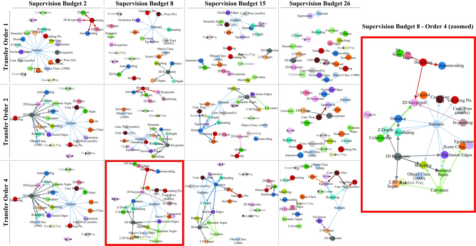
Figure 8: Computed taxonomies for solving 22 tasks given various supervision budgets (x-axes), and maximum allowed transfer orders (y-axes). One is magnified for better visibility. Nodes with incoming edges are target tasks, and the number of their incoming edges is the order of their chosen transfer function. Still transferring to some targets when tge budget is 26 (full budget) means certain transfers started performing better than their fully supervised task-specific counterpart. See the interactive solver website for color coding of the nodes by Gain and Quality metrics. Dimmed nodes are the source-only tasks, and thus, only participate in the taxonomy if found worthwhile by the BIP optimization to be one of the sources.

图 8：在给定各种监督预算（x 轴）和允许的最大转移指令（y 轴）的情况下，计算解决 22 项任务的分类法。 其中一个被放大以获得更好的可见性。 具有传入边的节点是目标任务，其传入边的数量是其选择的传递函数的阶数。 当 tge 预算为 26（全部预算）时，仍然转移到某些目标意味着某些转移开始比完全监督的特定任务对应对象表现得更好。 请参阅交互式求解器网站，了解按增益和质量指标对节点进行颜色编码。 变暗的节点是仅源任务，因此，仅当 BIP 优化发现值得作为源之一时才参与分类。

4 Experiments

4 实验

With 26 tasks in the dictionary (4 source-only tasks), our approach leads to training $26$ fully supervised task-specific networks, $22\times 25$ transfer networks in 1st order, and $22\times{25\choose k}$ for $k^{th}$ order, from which we sample according to the procedure in Sec. 3. The total number of transfer functions trained for the taxonomy was $\sim$3,000 which took 47,886 GPU hours on the cloud.

通过字典中的 26 个任务（4 个仅源任务），我们的方法导致训练$26$完全监督的特定于任务的网络、1st 顺序的$22\times 25$传输网络以及$k^{th}$顺序的 $22\times{25\choose k}$，我们根据第 2 节中的过程从中进行采样。 3. 为分类训练的传输函数总数为$\sim$3,000 个，在云上花费了 47,886 个 GPU 小时。

Out of 26 tasks, we usually use the following 4 as source-only tasks (described in Sec. 3) in the experiments: colorization, jigsaw puzzle, in-painting, random projection. However, the method is applicable to an arbitrary partitioning of the dictionary into $\mathcal{T}$ and $\mathcal{S}$. The interactive solver website allows the user to specify any desired partition.

在 26 个任务中，我们通常在实验中使用以下 4 个作为纯源任务（在第 3 节中描述）：着色、拼图、绘画、随机投影。 然而，该方法适用于将字典任意划分为$\mathcal{T}$和$\mathcal{S}$。 交互式求解器网站允许用户指定任何所需的分区。

Task	$avg$	$rand$	Task	$avg$	$rand$	Task	$avg$	$rand$
Denoising	100	99.9	Layout	99.6	89.1	Scene Class.	97.0	93.4
Autoenc.	100	99.8	2D Edges	100	99.9	Occ. Edges	100	95.4
Reshading	94.9	95.2	Pose (fix)	76.3	79.5	Pose (nonfix)	60.2	61.9
Inpainting	99.9	-	2D Segm.	97.7	95.7	2.5D Segm.	94.2	89.4
Curvature	78.7	93.4	Matching	86.8	84.6	Egomotion	67.5	72.3
Normals	99.4	99.5	Vanishing	99.5	96.4	2D Keypnt.	99.8	99.4
Z-Depth	92.3	91.1	Distance	92.4	92.1	3D Keypnt.	96.0	96.9
Mean	92.4	90.9

Table 1: Task-Specific Networks’ Sanity: Win rates vs. random (Gaussian) network representation readout and statistically informed guess $avg$.

任务	$avg$	$rand$	任务	$avg$	$rand$	任务	$avg$	$rand$
去噪	100	99.9	布局	99.6	89.1	场景类。	97.0	93.4
自动控制。	100	99.8	2D 边缘	100	99.9	奥克。 边缘	100	95.4
重新着色	94.9	95.2	姿势（固定）	76.3	79.5	姿势（非固定）	60.2	61.9
修复	99.9	-	2D 段。	97.7	95.7	2.5D 段。	94.2	89.4
曲率	78.7	93.4	匹配	86.8	84.6	自我运动	67.5	72.3
法线	99.4	99.5	消失	99.5	96.4	2D 按键。	99.8	99.4
Z 深度	92.3	91.1	距离	92.4	92.1	3D 关键点。	96.0	96.9
意思是	92.4	90.9

表 1：特定任务网络的健全性： 获胜率与随机（高斯）网络表示读出和统计信息猜测$avg$。

Network Architectures: We preserved the architectural and training details across tasks as homogeneously as possible to avoid injecting any bias. The encoder architecture is identical across all task-specific networks and is a fully convolutional ResNet-50 without pooling. All transfer functions include identical shallow networks with 2 conv layers (concatenated channel-wise if higher-order). The loss ($L_{t}$) and decoder’s architecture, though, have to depend on the task as the output structures of different tasks vary; for all pixel-to-pixel tasks, e.g. normal estimation, the decoder is a 15-layer fully convolutional network; for low dimensional tasks, e.g. vanishing points, it consists of 2-3 FC layers. All networks are trained using the same hyperparameters regardless of task and on exactly the same input images. Tasks with more than one input, e.g. relative camera pose, share weights between the encoder towers. Transfer networks are all trained using the same hyperparameters as the task-specific networks, except that we anneal the learning rate earlier since they train much faster. Detailed definitions of architectures, training process, and experiments with different encoders can be found in the supplementary material.

网络架构：我们尽可能均匀地保留跨任务的架构和训练细节，以避免注入任何偏差。 编码器架构在所有特定于任务的网络中都是相同的，并且是一个没有池化的完全卷积 ResNet-50。 所有 transfer 函数都包含具有 2 个卷积层的相同浅层网络（如果是高阶，则按通道连接）。 然而，损失（$L_{t}$）和解码器的架构必须取决于任务，因为不同任务的输出结构有所不同； 对于所有像素到像素的任务，例如 正常估计，解码器是15层全卷积网络； 对于低维任务，例如 消失点，由2-3个FC层组成。 无论任务如何，所有网络都使用相同的超参数并在完全相同的输入图像上进行训练。 具有多个输入的任务，例如 相对相机姿态，在编码器塔之间共享权重。 传输网络都是使用与特定任务网络相同的超参数进行训练的，只是我们更早地退火了学习率，因为它们训练得更快。 架构的详细定义、训练过程以及不同编码器的实验可以在补充材料中找到。

Data Splits: Our dataset includes 4 million images. We made publicly available the models trained on full dataset, but for the experiments reported in the main paper, we used a subset of the dataset as the extracted structure stabilized and did not change when using more data (explained in Sec. 5.2). The used subset is partitioned into training (120k), validation (16k), and test (17k) images, each from non-overlapping sets of buildings. Our task-specific networks are trained on the training set and the transfer networks are trained on a subset of validation set, ranging from 1k images to 16k, in order to model the transfer patterns under different data regimes. In the main paper, we report all results under the 16k transfer supervision regime ($\sim$10% of the split) and defer the additional sizes to the supplementary material and website (see Sec. 5.2). Transfer functions are evaluated on the test set.

数据分割： 我们的数据集包含 400 万张图像。 我们公开了在完整数据集上训练的模型，但对于主论文中报告的实验，我们使用了数据集的一个子集，因为提取的结构稳定并且在使用更多数据时没有改变（第 5.2 节中解释）。 使用的子集被划分为训练 (120k)、验证 (16k) 和测试 (17k) 图像，每个图像都来自非重叠的建筑物集。 我们的特定任务网络在训练集上进行训练，传输网络在验证集的子集上进行训练，范围从 1k 图像到 16k，以便对不同数据机制下的传输模式进行建模。 在主论文中，我们报告了 16k 传输监管制度下的所有结果（$\sim$ 分割的 10%），并将额外的大小推迟到补充材料和网站（参见第 5.2 节）。 传递函数在测试集上进行评估。

How good are the trained task-specific networks? Win rate (%) is the proportion of test set images for which a baseline is beaten. Table 1 provides win rates of the task-specifc networks vs. two baselines. Visual outputs for a random test sample are in Fig. 3. The high win rates in Table 1 and qualitative results show the networks are well trained and stable and can be relied upon for modeling the task space. See results of applying the networks on a YouTube video frame-by-frame here. A live demo for user uploaded queries is available here.

经过训练的特定任务网络有多好？ 获胜率 (%) 是测试集图像中基线被击败的比例。 表 1 提供了特定任务网络与两个基线的胜率。 随机测试样本的视觉输出如图 3 所示。表 1 中的高获胜率和定性结果表明网络训练有素且稳定，可以用来对任务空间进行建模。 在此查看在 YouTube 视频上逐帧应用网络的结果。 此处提供了用户上传查询的现场演示。

To get a sense of the quality of our networks vs. state-of-the-art task-specific methods, we compared our depth estimator vs. released models of [53] which led to outperforming [53] with a win rate of 88% and losses of 0.35 vs. 0.47 (further details in the supplementary material). In general, we found the task-specific networks to perform on par or better than state-of-the-art for many of the tasks, though we do not formally benchmark or claim this.

为了了解我们的网络的质量与最先进的特定任务方法的质量，我们将我们的深度估计器与[53]发布的模型进行了比较，该模型表现优于[53]，胜率为 88%，损失为 0.35 与 0.47（补充材料中的更多详细信息）。 总的来说，我们发现针对许多任务的特定任务网络的性能与最先进的网络相当或更好，尽管我们没有正式进行基准测试或声称这一点。

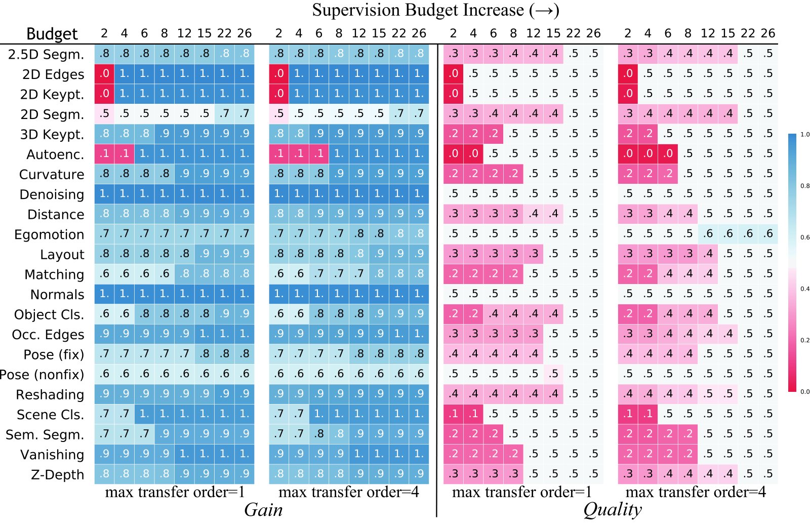
Figure 9: Evaluation of taxonomy computed for solving the full task dictionary. Gain (left) and Quality (right) values for each task using the policy suggested by the computed taxonomy, as the supervision budget increases($\rightarrow$). Shown for transfer orders 1 and 4.

图 9：为解决完整任务字典而计算的分类法评估。 随着监督预算的增加 ($\rightarrow$)，使用计算分类法建议的策略获得每项任务的增益（左）和质量（右）值。 显示的是转储订单 1 和 4。

4.1 Evaluation of Computed Taxonomies

4.1 对所计算分类学的评估

Fig. 8 shows the computed taxonomies optimized to solve the full dictionary, i.e. all tasks are placed in $\mathcal{T}$ and $\mathcal{S}$ (except for 4 source-only tasks that are in $\mathcal{S}$ only). This was done for various supervision budgets (columns) and maximum allowed order (rows) constraints. Still seeing transfers to some targets when the budget is 26 (full dictionary) means certain transfers became better than their fully supervised task-specific counterpart.

图 8 显示了为解决完整字典而优化的计算分类法，即所有任务都放置在$\mathcal{T}$和$\mathcal{S}$中（除了仅位于$\mathcal{S}$中的 4 个纯源任务）。 这是针对各种监督预算（列）和最大允许顺序（行）约束而完成的。 当预算为 26（完整字典）时，仍然看到某些目标的转移意味着某些转移变得比完全监督的特定任务对应物更好。

While Fig. 8 shows the structure and connectivity, Fig. 9 quantifies the results of taxonomy recommended transfer policies by two metrics of Gain and Quality, defined as:

图 8 显示了结构和连接性，而图 9 通过增益和质量两个指标量化了分类推荐的传输策略的结果，定义为：

Gain: win rate (%) against a network trained from scratch using the same training data as transfer networks’. That is, the best that could be done if transfer learning was not utilized. This quantifies the gained value by transferring. Quality: win rate (%) against a fully supervised network trained with 120k images (gold standard).

增益（Gain）：相对用与迁移网络相同训练数据、从零训练的网络的胜率（%）。即若不做迁移学习时的最好结果，用来量化迁移带来的收益。质量（Quality）：相对用 12 万张图全监督训练的网络（金标准）的胜率（%）。

Red (0) and Blue (1) represent outperforming the reference method on none and all of test set images, respectively (so the transition Red$\rightarrow$White$\rightarrow$Blue is desirable. White (.5) represents equal performance to reference).

红色 (0) 和蓝色 (1) 分别表示在没有或所有测试集图像上均优于参考方法（因此过渡红色$\rightarrow$白色$\rightarrow$蓝色是理想的。白色 (.5) 表示与参考具有相同的性能）。

Each column in Fig. 9 shows a supervision budget. As apparent, good results can be achieved even when the supervision budget is notably smaller than the number of solved tasks, and as the budget increases, results improve (expected). Results are shown for 2 maximum allowed orders.

图9中的每一列显示了监督预算。 显然，即使监督预算明显小于已解决的任务数量，也可以取得良好的结果，并且随着预算的增加，结果会改善（预期）。 显示 2 个最大允许订单的结果。

Task	scratch	ImageNet[51]	Wang.[96]	Agrawal.[1]	Zamir.[100]	Zhang.[103]	Noroozi.[68]	full sup.	Taxonomy
Depth	88	88	93	89	88	84	86	43	-
.03	.04	.04	.03	.04	.03	.03	.02	.02
Scene Cls.	80	52	83	74	74	71	75	15	-
3.30	2.76	3.56	3.15	3.17	3.09	3.19	2.23	2.63
Sem. Segm.	78	79	82	85	76	78	84	21	-
1.74	1.88	1.92	1.80	1.85	1.74	1.71	1.42	1.53
Object Cls.	79	54	82	76	75	76	76	34	-
4.08	3.57	4.27	3.99	3.98	4.00	3.97	3.26	3.46
Normals	97	98	98	98	98	97	97	6	-
.22	.30	.34	.28	.28	.23	.24	.12	.15
2.5D Segm.	80	93	92	89	90	84	87	40	-
.21	.34	.34	.26	.29	.22	.24	.16	.17
Occ. Edges	93	96	95	93	94	93	94	42	-
.16	.19	.18	.17	.18	.16	.17	.12	.13
Curvature	88	94	89	85	88	92	88	29	-
.25	.28	.26	.25	.26	.26	.25	.21	.22
Egomotion	79	78	83	77	76	74	71	59	-
8.60	8.58	9.26	8.41	8.34	8.15	7.94	7.32	6.85
Layout	80	76	85	79	77	78	70	36	-
.66	.66	.85	.65	.65	.62	.54	.37	.41

Figure 10: Generalization to Novel Tasks. Each row shows a novel test task. Left: Gain and Quality values using the devised “all-for-one” transfer policies for novel tasks for orders 1-4. Right: Win rates (%) of the transfer policy over various self-supervised methods, ImageNet features, and scratch are shown in the colored rows. Note the large margin of win by taxonomy. The uncolored rows show corresponding loss values.

任务	划痕	图像网[51]	王。[96]	阿格拉瓦尔。[1]	扎米尔。[100]	张。[103]	诺鲁兹。[68]	完全支持。	分类学
深度	88	88	93	89	88	84	86	43	-
.03	.04	.04	.03	.04	.03	.03	**.02 **	.02
场景分类。	80	52	83	74	74	71	75	15	-
3.30	2.76	3.56	3.15	3.17	3.09	3.19	** 2.23 **	2.63
Sem. Segm.	78	79	82	85	76	78	84	21	-
1.74	1.88	1.92	1.80	1.85	1.74	1.71	** 1.42 **	1.53
对象类别。	79	54	82	76	75	76	76	34	-
4.08	3.57	4.27	3.99	3.98	4.00	3.97	** 3.26 **	3.46
法线	97	98	98	98	98	97	97	6	-
.22	.30	.34	.28	.28	.23	.24	**.12 **	.15
2.5D 段。	80	93	92	89	90	84	87	40	-
.21	.34	.34	.26	.29	.22	.24	**.16 **	.17
奥克。 边缘	93	96	95	93	94	93	94	42	-
.16	.19	.18	.17	.18	.16	.17	.12	.13
曲率	88	94	89	85	88	92	88	29	-
.25	.28	.26	.25	.26	.26	.25	**.21 **	.22
自我运动	79	78	83	77	76	74	71	59	-
8.60	8.58	9.26	8.41	8.34	8.15	7.94	7.32	ypm6gvpyrxqa2sb2i1n3
布局	80	76	85	79	77	78	70	36	-
.66	.66	.85	.65	.65	.62	.54	wkhezu69d1yq05z93mem	.41

图 10：新任务的概括。 每行显示一个新颖的测试任务。 左：使用针对订单 1-4 的新任务设计的“一体式”转移策略的增益和质量值。 右图：传输策略相对于各种自监督方法、ImageNet 特征和暂存的胜率 (%) 显示在彩色行中。 请注意分类法的巨大优势。 未着色的行显示相应的损失值。

4.2 Generalization to Novel Tasks

4.2 泛化到新任务

The taxonomies in Sec. 4.1 were optimized for solving all tasks in the dictionary. In many situations, a practitioner is interested in a single task which even may not be in the dictionary. Here we evaluate how taxonomy transfers to a novel out-of-dictionary task with little data.

Sec 中的分类法。 4.1 针对解决字典中的所有任务进行了优化。 在许多情况下，从业者对单个任务感兴趣，而该任务甚至可能不在字典中。 在这里，我们评估分类学如何转移到数据很少的新颖的字典外任务。

This is done in an all-for-one scenario where we put one task in $\mathcal{T}$ and all others in $\mathcal{S}$. The task in $\mathcal{T}$ is target-only and has no task-specific network. Its limited data (16k) is used to train small transfer networks to sources. This basically localizes where the target would be in the taxonomy.

这是在全对一场景中完成的，我们将一项任务放入$\mathcal{T}$中，将所有其他任务放入$\mathcal{S}$中。$\mathcal{T}$中的任务仅是目标，没有特定于任务的网络。 其有限的数据（16k）用于训练小型传输网络到源。 这基本上“本地化”了目标在分类中的位置。

Fig. 10 (left) shows the Gain and Quality of the transfer policy found by the BIP for each task. Fig. 10 (right) compares the taxonomy suggested policy against some of the best existing self-supervised methods [96, 103, 68, 100, 1], ImageNet FC7 features [51], training from scratch, and a fully supervised network (gold standard).

图 10（左）显示了 BIP 为每个任务找到的传输策略的增益和质量。 图 10（右）将分类建议的策略与一些现有的最佳自监督方法 [96,103,68,100,1]、ImageNet FC7 特征 [51]、从头开始训练和完全监督网络（黄金标准）进行了比较。

The results in Fig. 10 (right) are noteworthy. The large win margin for taxonomy shows that carefully selecting transfer policies depending on the target is superior to fixed transfers, such as the ones employed by self-supervised methods. ImageNet features which are the most popular off-the-shelf features in vision are also outperformed by those policies. Additionally, though the taxonomy transfer policies lose to fully supervised networks (gold standard) in most cases, the results often get close with win rates in 40% range. These observations suggests the space has a rather predicable and strong structure. For graph visualization of the all-for-one taxonomy policies please see the supplementary material. The solver website allows generating the taxonomy for arbitrary sets of target-only tasks.

图 10（右）中的结果值得注意。 分类学的巨大赢利表明，根据目标仔细选择转移策略优于固定转移，例如自我监督方法所采用的转移策略。 ImageNet 特征是视觉领域最流行的现成特征，这些策略的性能也优于这些特征。 此外，尽管在大多数情况下分类转移策略输给了完全监督的网络（黄金标准），但结果通常接近于 40% 范围内的获胜率。 这些观察结果表明该空间具有相当可预测且坚固的结构。 有关全合一分类政策的图形可视化，请参阅补充材料。 求解器网站允许为任意一组仅目标任务生成分类法。

5 Significance Test of the Structure

5 结构的显著性检验

The previous evaluations showed good transfer results in terms of Quality and Gain, but how crucial is it to use our taxonomy to choose smart transfers over just choosing any transfer? In other words, how significant/strong is the discovered structure of task space? Fig. 11 quantifies this by showing the performance of our taxonomy versus a large set of taxonomies with random connectivities. Our taxonomy outperformed all other connectivities by a large margin signifying both existence of a strong structure in the space as well as a good modeling of it by our approach. Complete experimental details is available in supplementary material.

之前的评估在质量和增益方面显示了良好的转移结果，但是使用我们的分类法选择智能转移而不是仅选择任何转移有多重要？ 换句话说，所发现的任务空间结构有多“显着/强”？ 图 11 通过显示我们的分类法与大量具有随机连接的分类法的性能来量化这一点。 我们的分类法大大优于所有其他连接性，这表明该空间中存在强大的结构，并且通过我们的方法对其进行了良好的建模。 完整的实验细节可在补充材料中找到。

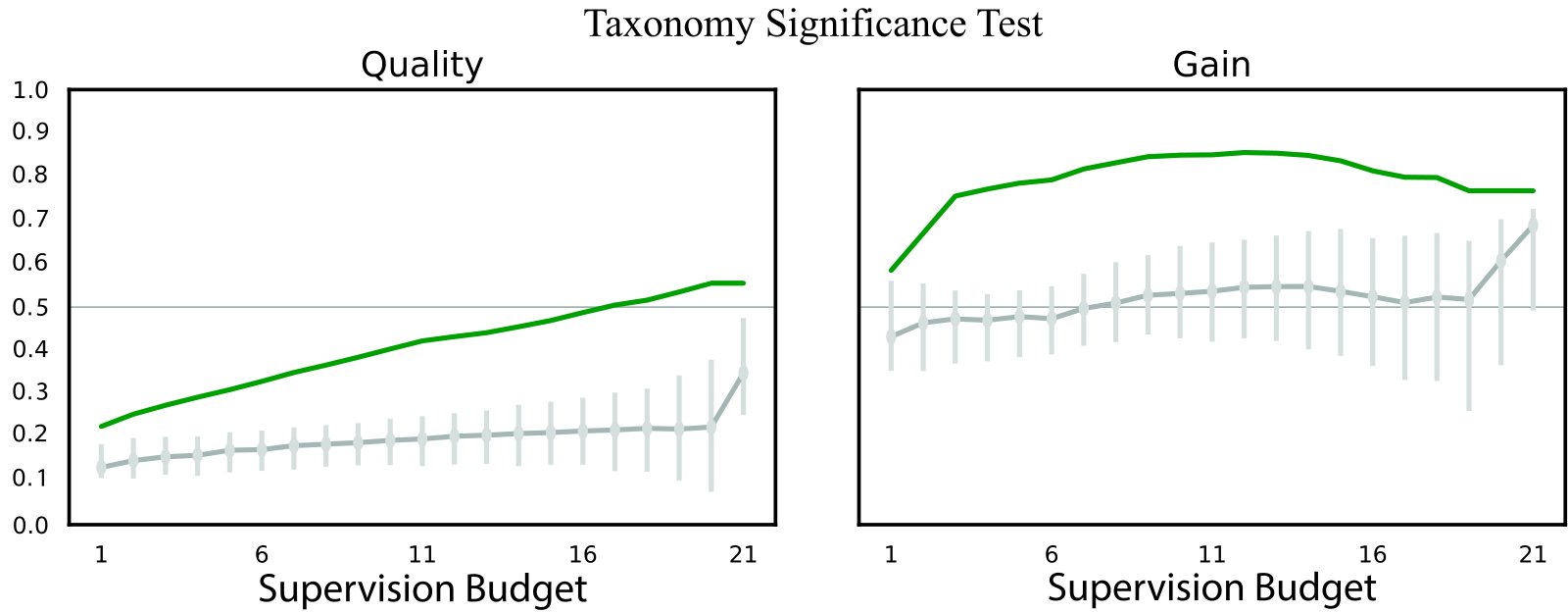
Figure 11: Structure Significance. Our taxonomy compared with random transfer policies (random feasible taxonomies that use the maximum allowable supervision budget). Y-axis shows Quality or Gain, and X-axis is the supervision budget. Green and gray represent our taxonomy and random connectivities, respectively. Error bars denote 5th*–95*th percentiles.**

图 11：结构意义。 我们的分类法与随机转移政策（使用最大允许监督预算的随机可行分类法）进行了比较。 Y 轴显示质量或增益*，X 轴是监督预算。 绿色和灰色分别代表我们的分类和随机连接。 误差线表示第 5*th–95th 个百分位数**。

5.1 Evaluation on MIT Places & ImageNet

5.1 在 MIT Places 与 ImageNet 上的评估

To what extent are our findings dataset dependent, and would the taxonomy change if done on another dataset? We examined this by finding the ranking of all tasks for transferring to two target tasks of object classification and scene classification on our dataset. We then fine tuned our task-specific networks on other datasets (MIT Places [104] for scene classification, ImageNet [78] for object classification) and evaluated them on their respective test sets and metrics. Fig. 12 shows how the results correlate with taxonomy’s ranking from our dataset. The Spearman’s rho between the taxonomy ranking and the Top-1 ranking is 0.857 on Places and 0.823 on ImageNet showing a notable correlation. See supplementary material for complete experimental details.

我们的研究结果在多大程度上依赖于数据集？如果在另一个数据集上进行分类，分类法会改变吗？ 我们通过查找所有任务的排名来检查这一点，以转移到数据集上的对象分类和场景分类这两个目标任务。 然后，我们在其他数据集（用于场景分类的 MIT Places [104]，用于对象分类的 ImageNet [78]）上微调我们的特定任务网络，并根据各自的测试集和指标对其进行评估。 图 12 显示了结果如何与我们数据集中的分类排名相关。 分类排名与 Top-1 排名之间的 Spearman rho 在 Places 上为 0.857，在 ImageNet 上为 0.823，显示出显着的相关性。 有关完整的实验细节，请参阅补充材料。

5.2 Universality of the Structure

5.2 结构的普适性

We employed a computational approach with various design choices. It is important to investigate how specific to those the discovered structure is. We did stability tests by computing the variance in our output when making changes in one of the following system choices: I. architecture of task-specific networks, II. architecture of transfer function networks, III. amount of data available for training transfer networks, IV. datasets, V. data splits, VI. choice of dictionary. Overall, despite injecting large changes (e.g. varying the size of training data of transfer functions by 16x, size and architecture of task-specific networks and transfer networks by 4x), we found the outputs to be remarkably stable leading to almost no change in the output taxonomy computed on top. Detailed results and experimental setup of each tests are reported in the supplementary material.

我们采用了具有各种设计选择的计算方法。 研究所发现的结构的特异性非常重要。 我们通过计算在更改以下系统选择之一时输出的方差来进行稳定性测试：I。 特定任务网络的体系结构，II。 传递函数网络的体系结构，III。 可用于训练传输网络的数据量，IV。 数据集，V. 数据分割，VI。 字典的选择。 总体而言，尽管注入了巨大的变化（例如，将传递函数的训练数据大小改变 16 倍，将特定于任务的网络和传递网络的大小和架构改变 4 倍），但我们发现输出非常稳定，导致顶部计算的输出分类几乎没有变化。 补充材料中报告了每个测试的详细结果和实验设置。

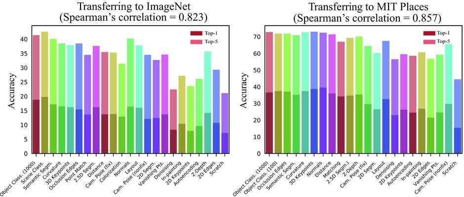
Figure 12: Evaluating the discovered structure on other datasets: ImageNet [78] (left) for object classification and MIT Places [104] (right) for scene classification. Y-axis shows accuracy on the external benchmark while bars on x-axis are ordered by taxonomy’s predicted performance based on our dataset. A monotonically decreasing plot corresponds to preserving identical orders and perfect generalization.

图 12：评估其他数据集上发现的结构：用于对象分类的 ImageNet [78]（左）和用于场景分类的 MIT Places [104]（右）。 Y 轴显示外部基准的准确性，而 x 轴上的条形则根据基于我们的数据集的分类法预测性能进行排序。 单调递减图对应于保留相同的阶数和完美的泛化。

5.3 Task Similarity Tree

5.3 任务相似树

Thus far we showed the task space has a structure, measured this structure, and presented its utility for transfer learning via devising transfer policies. This structure can be presented in other manners as well, e.g. via a metric of similarity across tasks. Figure 13 shows a similarity tree for the tasks in our dictionary. This is acquired from agglomerative clustering of the tasks based on their transferring-out behavior, i.e. using columns of normalized affinity matrix $P$ as feature vectors for tasks. The tree shows how tasks would be hierarchically positioned w.r.t. to each other when measured based on providing information for solving other tasks; the closer two tasks, the more similar their role in transferring to other tasks. Notice that the 3D, 2D, low dimensional geometric, and semantic tasks are found to cluster together using a fully computational approach, which matches the intuitive expectations from the structure of task space. The transfer taxonomies devised by BIP are consistent with this tree as BIP picks the sources in a way that all of these modes are quantitatively best covered, subject to the given budget and desired target set.

到目前为止，我们展示了任务空间有一个结构，测量了这个结构，并通过设计迁移策略展示了它对于迁移学习的效用。 该结构也可以以其他方式呈现，例如 通过任务之间的相似性度量。 图 13 显示了字典中任务的相似性树。 这是根据任务的转出行为从任务的凝聚聚类中获得的，即使用归一化亲和力矩阵$P$的列作为任务的特征向量。 该树显示了任务如何分层定位。 基于提供解决其他任务的信息进行衡量； 两个任务越接近，它们在转移到其他任务时的角色就越相似。 请注意，3D、2D、低维几何和语义任务被发现使用完全计算方法聚集在一起，这符合任务空间结构的直观期望。 BIP 设计的转移分类法与该树一致，因为 BIP 根据给定的预算和期望的目标集，以定量最佳覆盖所有这些模式的方式选择来源。

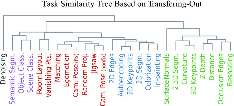
Figure 13: Task Similarity Tree. Agglomerative clustering of tasks based on their transferring-out patterns (i.e. using columns of normalized affinity matrix as task features). 3D, 2D, low dimensional geometric, and semantic tasks clustered together using a fully computational approach.

图 13：任务相似性树。 基于任务的转出模式对任务进行凝聚聚类（即使用归一化亲和力矩阵的列作为任务特征）。 使用完全计算方法将 3D、2D、低维几何和语义任务聚集在一起。

6 Limitations and Discussion

6 局限与讨论

We presented a method for modeling the space of visual tasks by way of transfer learning and showed its utility in reducing the need for supervision. The space of tasks is an interesting object of study in its own right and we have only scratched the surface in this regard. We also made a number of assumptions in the framework which should be noted.

我们提出了一种通过迁移学习对视觉任务空间进行建模的方法，并展示了其在减少监督需求方面的实用性。 任务空间本身就是一个有趣的研究对象，我们在这方面只触及了表面。 我们还在框架中做出了一些值得注意的假设。

Model Dependence: We used a computational approach and adopted neural networks as our function class. Though we validated the stability of the findings w.r.t various architectures and datasets, it should be noted that the findings are in principle model and data specific.

*模型依赖性：*我们使用计算方法并采用神经网络作为我们的函数类。 尽管我们验证了研究结果在各种架构和数据集上的稳定性，但应该注意的是，这些研究结果原则上是模型和数据特定的。

Compositionality: We performed the modeling via a set of common human-defined visual tasks. It is natural to consider a further compositional approach in which such common tasks are viewed as observed samples which are composed of computationally found latent subtasks.

*组合性：*我们通过一组常见的人类定义的视觉任务来执行建模。 很自然地考虑一种进一步的组合方法，其中这些常见任务被视为“观察到的样本”，它们由计算发现的潜在子任务组成。

Space Regularity: We performed modeling of a dense space via a sampled dictionary. Though we showed a good tolerance w.r.t. to the choice of dictionary and transferring to out-of-dictionary tasks, this outcome holds upon a proper sampling of the space as a function of its regularity. More formal studies on properties of the computed space is required for this to be provably guaranteed for a general case.

*空间规律性：*我们通过采样字典对密集空间进行建模。 尽管我们表现出了良好的容忍度。 对于字典的选择和转移到字典外的任务，这个结果取决于对空间的适当采样作为其规律性的函数。 需要对计算空间的属性进行更正式的研究，才能在一般情况下证明这一点。

Transferring to Non-visual and Robotic Tasks: Given the structure of the space of visual tasks and demonstrated transferabilities to novel tasks, it is worthwhile to question how this can be employed to develop a perception module for solving downstream tasks which are not entirely visual, e.g. robotic manipulation, but entail solving a set of (a priori unknown) visual tasks.

*转移到非视觉和机器人任务：*考虑到视觉任务空间的结构以及对新任务的可转移性，值得质疑的是如何利用它来开发感知模块来解决不完全视觉的下游任务，例如 机器人操作，但需要解决一组（先验未知的）视觉任务。

Lifelong Learning: We performed the modeling in one go. In many cases, e.g. lifelong learning, the system is evolving and the number of mastered tasks constantly increase. Such scenarios require augmentation of the structure with expansion mechanisms based on new beliefs. Acknowledgement: We acknowledge the support of NSF (DMS-1521608), MURI (1186514-1-TBCJE), ONR MURI (N00014-14-1-0671), Toyota(1191689-1-UDAWF), ONR MURI (N00014-13-1-0341), Nvidia, Tencent, a gift by Amazon Web Services, a Google Focused Research Award.

终身学习：我们一次性完成了建模。 在许多情况下，例如 终身学习，系统不断发展，掌握的任务数量不断增加。 这种情况需要使用基于新信念的扩展机制来增强结构。 致谢： 我们感谢 NSF (DMS-1521608)、MURI (1186514-1-TBCJE)、ONR MURI (N00014-14-1-0671)、Toyota (1191689-1-UDAWF)、ONR MURI (N00014-13-1-0341)、Nvidia、腾讯的支持， 亚马逊网络服务，谷歌重点研究奖。

References

参考文献

[1] P. Agrawal, J. Carreira, and J. Malik. Learning to see by moving. In Proceedings of the IEEE International Conference on Computer Vision , pages 37–45, 2015.

[2] M. Andrychowicz, M. Denil, S. Gomez, M. W. Hoffman, D. Pfau, T. Schaul, and N. de Freitas. Learning to learn by gradient descent by gradient descent. In Advances in Neural Information Processing Systems , pages 3981–3989, 2016.

[3] I. Armeni, S. Sax, A. R. Zamir, and S. Savarese. Joint 2d-3d-semantic data for indoor scene understanding. arXiv preprint arXiv:1702.01105 , 2017.

[4] S. Arora, A. Bhaskara, R. Ge, and T. Ma. Provable bounds for learning some deep representations. In International Conference on Machine Learning , pages 584–592, 2014.

[5] Y. Aytar and A. Zisserman. Tabula rasa: Model transfer for object category detection. In Computer Vision (ICCV), 2011 IEEE International Conference on , pages 2252–2259. IEEE, 2011.

[6] J. Baxter. A bayesian/information theoretic model of learning to learn viamultiple task sampling. Mach. Learn. , 28(1):7–39, July 1997.

[7] S. Ben-David and R. S. Borbely. A notion of task relatedness yielding provable multiple-task learning guarantees. Machine Learning , 73(3):273–287, Dec 2008.

[8] Y. Bengio, A. Courville, and P. Vincent. Representation learning: A review and new perspectives. IEEE transactions on pattern analysis and machine intelligence , 35(8):1798–1828, 2013.

[9] P. Berkhin et al. A survey of clustering data mining techniques. Grouping multidimensional data , 25:71, 2006.

[10] E. Bienenstock, S. Geman, and D. Potter. Compositionality, mdl priors, and object recognition. In Advances in neural information processing systems , pages 838–844, 1997.

[11] H. Bilen and A. Vedaldi. Integrated perception with recurrent multi-task neural networks. In Advances in neural information processing systems , pages 235–243, 2016.

[12] J. Bingel and A. Søgaard. Identifying beneficial task relations for multi-task learning in deep neural networks. arXiv preprint arXiv:1702.08303 , 2017.

[13] O. Boiman and M. Irani. Similarity by composition. In Advances in neural information processing systems , pages 177–184, 2007.

[14] A. Chang, A. Dai, T. Funkhouser, M. Halber, M. Nießner, M. Savva, S. Song, A. Zeng, and Y. Zhang. Matterport3d: Learning from rgb-d data in indoor environments. arXiv preprint arXiv:1709.06158 , 2017.

[15] Z. Chen and B. Liu. Lifelong Machine Learning . Morgan & Claypool Publishers, 2016.

[16] I. I. CPLEX. V12. 1: User’s manual for cplex. International Business Machines Corporation , 46(53):157, 2009.

[17] C. Doersch, A. Gupta, and A. A. Efros. Unsupervised visual representation learning by context prediction. In Proceedings of the IEEE International Conference on Computer Vision , pages 1422–1430, 2015.

[18] C. Doersch and A. Zisserman. Multi-task self-supervised visual learning. arXiv preprint arXiv:1708.07860 , 2017.

[19] J. Donahue, Y. Jia, O. Vinyals, J. Hoffman, N. Zhang, E. Tzeng, and T. Darrell. Decaf: A deep convolutional activation feature for generic visual recognition. In International conference on machine learning , pages 647–655, 2014.

[20] J. Donahue, P. Krähenbühl, and T. Darrell. Adversarial feature learning. arXiv preprint arXiv:1605.09782 , 2016.

[21] Y. Duan, J. Schulman, X. Chen, P. L. Bartlett, I. Sutskever, and P. Abbeel. Rl2: Fast reinforcement learning via slow reinforcement learning. arXiv preprint arXiv:1611.02779 , 2016.

[22] D. Erhan, Y. Bengio, A. Courville, P.-A. Manzagol, P. Vincent, and S. Bengio. Why does unsupervised pre-training help deep learning? Journal of Machine Learning Research , 11(Feb):625–660, 2010.

[23] A. Faktor and M. Irani. “clustering by composition”–unsupervised discovery of image categories. In European Conference on Computer Vision , pages 474–487. Springer, 2012.

[24] L. Fe-Fei et al. A bayesian approach to unsupervised one-shot learning of object categories. In Computer Vision, 2003. Proceedings. Ninth IEEE International Conference on , pages 1134–1141. IEEE, 2003.

[25] L. Fei-Fei, R. Fergus, and P. Perona. One-shot learning of object categories. IEEE transactions on pattern analysis and machine intelligence , 28(4):594–611, 2006.

[26] B. Fernando, A. Habrard, M. Sebban, and T. Tuytelaars. Unsupervised visual domain adaptation using subspace alignment. In Proceedings of the IEEE international conference on computer vision , pages 2960–2967, 2013.

[27] C. Finn, P. Abbeel, and S. Levine. Model-agnostic meta-learning for fast adaptation of deep networks. arXiv preprint arXiv:1703.03400 , 2017.

[28] C. Finn, S. Levine, and P. Abbeel. Guided cost learning: Deep inverse optimal control via policy optimization. CoRR , abs/1603.00448, 2016.

[29] C. Finn, X. Y. Tan, Y. Duan, T. Darrell, S. Levine, and P. Abbeel. Deep spatial autoencoders for visuomotor learning. In Robotics and Automation (ICRA), 2016 IEEE International Conference on , pages 512–519. IEEE, 2016.

[30] C. Finn, T. Yu, J. Fu, P. Abbeel, and S. Levine. Generalizing skills with semi-supervised reinforcement learning. CoRR , abs/1612.00429, 2016.

[31] C. Finn, T. Yu, T. Zhang, P. Abbeel, and S. Levine. One-shot visual imitation learning via meta-learning. CoRR , abs/1709.04905, 2017.

[32] I. K. Fodor. A survey of dimension reduction techniques. Technical report, Lawrence Livermore National Lab., CA (US), 2002.

[33] R. M. French. Catastrophic forgetting in connectionist networks: Causes, consequences and solutions. Trends in Cognitive Sciences , 3(4):128–135, 1999.

[34] R. Ge. Provable algorithms for machine learning problems . PhD thesis, Princeton University, 2013.

[35] S. Geman, D. F. Potter, and Z. Chi. Composition systems. Quarterly of Applied Mathematics , 60(4):707–736, 2002.

[36] R. Gopalan, R. Li, and R. Chellappa. Domain adaptation for object recognition: An unsupervised approach. In Computer Vision (ICCV), 2011 IEEE International Conference on , pages 999–1006. IEEE, 2011.

[37] A. Gopnik, C. Glymour, D. Sobel, L. Schulz, T. Kushnir, and D. Danks. A theory of causal learning in children: Causal maps and bayes nets. 111:3–32, 02 2004.

[38] A. Gopnik, C. Glymour, D. M. Sobel, L. E. Schulz, T. Kushnir, and D. Danks. A theory of causal learning in children: causal maps and bayes nets. Psychological review , 111(1):3, 2004.

[39] A. Gopnik, A. N. Meltzoff, and P. K. Kuhl. The scientist in the crib: Minds, brains, and how children learn. William Morrow & Co, 1999.

[40] A. Graves, G. Wayne, and I. Danihelka. Neural turing machines. CoRR , abs/1410.5401, 2014.

[41] I. Gurobi Optimization. Gurobi optimizer reference manual, 2016.

[42] K. Henry. The theory and applications of homomorphic cryptography. Master’s thesis, University of Waterloo, 2008.

[43] G. Hinton, O. Vinyals, and J. Dean. Distilling the knowledge in a neural network. arXiv preprint arXiv:1503.02531 , 2015.

[44] J. Hoffman, T. Darrell, and K. Saenko. Continuous manifold based adaptation for evolving visual domains. In Proceedings of the IEEE Conference on Computer Vision and Pattern Recognition , pages 867–874, 2014.

[45] Y. Hoshen and S. Peleg. Visual learning of arithmetic operations. CoRR , abs/1506.02264, 2015.

[46] F. Hu, G.-S. Xia, J. Hu, and L. Zhang. Transferring deep convolutional neural networks for the scene classification of high-resolution remote sensing imagery. Remote Sensing , 7(11):14680–14707, 2015.

[47] I.-H. Jhuo, D. Liu, D. Lee, and S.-F. Chang. Robust visual domain adaptation with low-rank reconstruction. In Computer Vision and Pattern Recognition (CVPR), 2012 IEEE Conference on , pages 2168–2175. IEEE, 2012.

[48] D. P. Kingma and J. Ba. Adam: A method for stochastic optimization. CoRR , abs/1412.6980, 2014.

[49] D. P. Kingma and M. Welling. Auto-encoding variational bayes. arXiv preprint arXiv:1312.6114 , 2013.

[50] I. Kokkinos. Ubernet: Training auniversal’convolutional neural network for low-, mid-, and high-level vision using diverse datasets and limited memory. arXiv preprint arXiv:1609.02132 , 2016.

[51] A. Krizhevsky, I. Sutskever, and G. E. Hinton. Imagenet classification with deep convolutional neural networks. In NIPS , pages 1097–1105, 2012.

[52] B. Kulis, K. Saenko, and T. Darrell. What you saw is not what you get: Domain adaptation using asymmetric kernel transforms. In Computer Vision and Pattern Recognition (CVPR), 2011 IEEE Conference on , pages 1785–1792. IEEE, 2011.

[53] I. Laina, C. Rupprecht, V. Belagiannis, F. Tombari, and N. Navab. Deeper depth prediction with fully convolutional residual networks. In 3D Vision (3DV), 2016 Fourth International Conference on , pages 239–248. IEEE, 2016.

[54] B. M. Lake, R. Salakhutdinov, and J. B. Tenenbaum. Human-level concept learning through probabilistic program induction. Science , 350(6266):1332–1338, 2015.

[55] B. M. Lake, T. D. Ullman, J. B. Tenenbaum, and S. J. Gershman. Building machines that learn and think like people. Behavioral and Brain Sciences , pages 1–101, 2016.

[56] Y. Li, H. Qi, J. Dai, X. Ji, and Y. Wei. Fully convolutional instance-aware semantic segmentation. arXiv preprint arXiv:1611.07709 , 2016.

[57] T.-Y. Lin, M. Maire, S. Belongie, J. Hays, P. Perona, D. Ramanan, P. Dollár, and C. L. Zitnick. Microsoft coco: Common objects in context. In European conference on computer vision , pages 740–755. Springer, 2014.

[58] F. Liu, G. Lin, and C. Shen. CRF learning with CNN features for image segmentation. CoRR , abs/1503.08263, 2015.

[59] Z. Luo, Y. Zou, J. Hoffman, and L. F. Fei-Fei. Label efficient learning of transferable representations acrosss domains and tasks. In Advances in Neural Information Processing Systems , pages 164–176, 2017.

[60] M. M. H. Mahmud. On Universal Transfer Learning , pages 135–149. Springer Berlin Heidelberg, Berlin, Heidelberg, 2007.

[61] J. Malik, P. Arbeláez, J. Carreira, K. Fragkiadaki, R. Girshick, G. Gkioxari, S. Gupta, B. Hariharan, A. Kar, and S. Tulsiani. The three r’s of computer vision: Recognition, reconstruction and reorganization. Pattern Recognition Letters , 72:4–14, 2016.

[62] N. Masuda, M. A. Porter, and R. Lambiotte. Random walks and diffusion on networks. Physics Reports , 716-717:1 – 58, 2017. Random walks and diffusion on networks.

[63] M. Mccloskey and N. J. Cohen. Catastrophic interference in connectionist networks: The sequential learning problem. The Psychology of Learning and Motivation , 24, 1989.

[64] L. Mihalkova, T. Huynh, and R. J. Mooney. Mapping and revising markov logic networks for transfer learning. In AAAI , volume 7, pages 608–614, 2007.

[65] T. Mikolov, Q. V. Le, and I. Sutskever. Exploiting similarities among languages for machine translation. CoRR , abs/1309.4168, 2013.

[66] I. Misra, A. Shrivastava, A. Gupta, and M. Hebert. Cross-stitch networks for multi-task learning. In Proceedings of the IEEE Conference on Computer Vision and Pattern Recognition , pages 3994–4003, 2016.

[67] A. Niculescu-Mizil and R. Caruana. Inductive transfer for bayesian network structure learning. In Artificial Intelligence and Statistics , pages 339–346, 2007.

[68] M. Noroozi and P. Favaro. Unsupervised learning of visual representations by solving jigsaw puzzles. In European Conference on Computer Vision , pages 69–84. Springer, 2016.

[69] M. Noroozi, H. Pirsiavash, and P. Favaro. Representation learning by learning to count. arXiv preprint arXiv:1708.06734 , 2017.

[70] M. Norouzi, T. Mikolov, S. Bengio, Y. Singer, J. Shlens, A. Frome, G. S. Corrado, and J. Dean. Zero-shot learning by convex combination of semantic embeddings. arXiv preprint arXiv:1312.5650 , 2013.

[71] M. Ovsjanikov, M. Ben-Chen, J. Solomon, A. Butscher, and L. Guibas. Functional maps: a flexible representation of maps between shapes. ACM Transactions on Graphics (TOG) , 31(4):30, 2012.

[72] D. Pathak, P. Krahenbuhl, J. Donahue, T. Darrell, and A. A. Efros. Context encoders: Feature learning by inpainting. In Proceedings of the IEEE Conference on Computer Vision and Pattern Recognition , pages 2536–2544, 2016.

[73] A. Pentina and C. H. Lampert. Multi-task learning with labeled and unlabeled tasks. stat , 1050:1, 2017.

[74] J. Piaget and M. Cook. The origins of intelligence in children , volume 8. International Universities Press New York, 1952.

[75] L. Y. Pratt. Discriminability-based transfer between neural networks. In Advances in neural information processing systems , pages 204–211, 1993.

[76] S. R. Richter, Z. Hayder, and V. Koltun. Playing for benchmarks. In International Conference on Computer Vision (ICCV) , 2017.

[77] S. T. Roweis and L. K. Saul. Nonlinear dimensionality reduction by locally linear embedding. science , 290(5500):2323–2326, 2000.

[78] O. Russakovsky, J. Deng, H. Su, J. Krause, S. Satheesh, S. Ma, Z. Huang, A. Karpathy, A. Khosla, M. Bernstein, et al. Imagenet large scale visual recognition challenge. International Journal of Computer Vision , 115(3):211–252, 2015.

[79] R. W. Saaty. The analytic hierarchy process – what it is and how it is used. Mathematical Modeling , 9(3-5):161–176, 1987.

[80] K. Saenko, B. Kulis, M. Fritz, and T. Darrell. Adapting visual category models to new domains. Computer Vision–ECCV 2010 , pages 213–226, 2010.

[81] R. Salakhutdinov, J. Tenenbaum, and A. Torralba. One-shot learning with a hierarchical nonparametric bayesian model. In Proceedings of ICML Workshop on Unsupervised and Transfer Learning , pages 195–206, 2012.

[82] J. Schulman, S. Levine, P. Moritz, M. I. Jordan, and P. Abbeel. Trust region policy optimization. CoRR , abs/1502.05477, 2015.

[83] A. Sharif Razavian, H. Azizpour, J. Sullivan, and S. Carlsson. Cnn features off-the-shelf: an astounding baseline for recognition. In Proceedings of the IEEE conference on computer vision and pattern recognition workshops , pages 806–813, 2014.

[84] D. L. Silver and K. P. Bennett. Guest editor’s introduction: special issue on inductive transfer learning. Machine Learning , 73(3):215–220, 2008.

[85] D. L. Silver, Q. Yang, and L. Li. Lifelong machine learning systems: Beyond learning algorithms. In in AAAI Spring Symposium Series , 2013.

[86] R. Socher, M. Ganjoo, C. D. Manning, and A. Ng. Zero-shot learning through cross-modal transfer. In NIPS , pages 935–943, 2013.

[87] N. Srivastava, G. Hinton, A. Krizhevsky, I. Sutskever, and R. Salakhutdinov. Dropout: A simple way to prevent neural networks from overfitting. Journal of Machine Learning Research , 15:1929–1958, 2014.

[88] C. Szegedy, W. Zaremba, I. Sutskever, J. Bruna, D. Erhan, I. J. Goodfellow, and R. Fergus. Intriguing properties of neural networks. CoRR , abs/1312.6199, 2013.

[89] J. B. Tenenbaum and T. L. Griffiths. Generalization, similarity, and bayesian inference. Behavioral and Brain Sciences , 24(4):629–640, 2001.

[90] J. B. Tenenbaum, C. Kemp, T. L. Griffiths, and N. D. Goodman. How to grow a mind: Statistics, structure, and abstraction. science , 331(6022):1279–1285, 2011.

[91] J. B. Tenenbaum, C. Kemp, and P. Shafto. Theory-based bayesian models of inductive learning and reasoning. In Trends in Cognitive Sciences , pages 309–318, 2006.

[92] D. G. R. Tervo, J. B. Tenenbaum, and S. J. Gershman. Toward the neural implementation of structure learning. Current opinion in neurobiology , 37:99–105, 2016.

[93] C. Tessler, S. Givony, T. Zahavy, D. J. Mankowitz, and S. Mannor. A deep hierarchical approach to lifelong learning in minecraft. In AAAI , pages 1553–1561, 2017.

[94] S. Thrun and L. Pratt. Learning to learn . Springer Science & Business Media, 2012.

[95] A. M. Turing. Computing machinery and intelligence. Mind , 59(236):433–460, 1950.

[96] X. Wang and A. Gupta. Unsupervised learning of visual representations using videos. In Proceedings of the IEEE International Conference on Computer Vision , pages 2794–2802, 2015.

[97] X. Wang, K. He, and A. Gupta. Transitive invariance for self-supervised visual representation learning. arXiv preprint arXiv:1708.02901 , 2017.

[98] T. Winograd. Thinking machines: Can there be? Are we , volume 200. University of California Press, Berkeley, 1991.

[99] J. Yang, R. Yan, and A. G. Hauptmann. Adapting svm classifiers to data with shifted distributions. In Data Mining Workshops, 2007. ICDM Workshops 2007. Seventh IEEE International Conference on , pages 69–76. IEEE, 2007.

[100] A. R. Zamir, T. Wekel, P. Agrawal, C. Wei, J. Malik, and S. Savarese. Generic 3d representation via pose estimation and matching. In European Conference on Computer Vision , pages 535–553. Springer, 2016.

[101] A. R. Zamir, F. Xia, J. He, A. Sax, J. Malik, and S. Savarese. Gibson Env: Real-world perception for embodied agents. In 2018 IEEE Conference on Computer Vision and Pattern Recognition (CVPR) . IEEE, 2018.

[102] C. Zhang, S. Bengio, M. Hardt, B. Recht, and O. Vinyals. Understanding deep learning requires rethinking generalization. CoRR , abs/1611.03530, 2016.

[103] R. Zhang, P. Isola, and A. A. Efros. Colorful image colorization. In European Conference on Computer Vision , pages 649–666. Springer, 2016.

[104] B. Zhou, A. Lapedriza, J. Xiao, A. Torralba, and A. Oliva. Learning deep features for scene recognition using places database. In Advances in neural information processing systems , pages 487–495, 2014.