Tacotron: Towards End-to-End Speech Synthesis

Tacotron：迈向端到端语音合成

Yuxuan Wang Thanks:  These authors really like tacos.    RJ Skerry-Ryan    Daisy Stanton    Yonghui Wu    Ron J. Weiss Thanks:  These authors would prefer sushi.    Navdeep Jaitly    Zongheng Yang    Ying Xiao    Zhifeng Chen    Samy Bengio    Quoc Le    Yannis Agiomyrgiannakis    Rob Clark    Rif A. SaurousGoogle, Inc. {yxwang,rjryan,rif}@google.com

Abstract

摘要

A text-to-speech synthesis system typically consists of multiple stages, such as a text analysis frontend, an acoustic model and an audio synthesis module. Building these components often requires extensive domain expertise and may contain brittle design choices. In this paper, we present Tacotron, an end-to-end generative text-to-speech model that synthesizes speech directly from characters. Given $<$text, audio$>$ pairs, the model can be trained completely from scratch with random initialization. We present several key techniques to make the sequence-to-sequence framework perform well for this challenging task. Tacotron achieves a 3.82 subjective 5-scale mean opinion score on US English, outperforming a production parametric system in terms of naturalness. In addition, since Tacotron generates speech at the frame level, it’s substantially faster than sample-level autoregressive methods.

文本转语音（TTS）系统通常由文本分析前端、声学模型与音频合成模块等多级流水线构成。搭建这些部件往往依赖大量领域经验，设计选择也容易发脆。本文提出 Tacotron：端到端生成式 TTS 模型，可直接从字符合成语音。给定 $<$文本, 音频$>$ 对，模型可从随机初始化完全从头训练。我们给出若干关键技巧，使序列到序列框架胜任这一困难任务。在美式英语上，Tacotron 的 5 分制主观平均意见分为 3.82，自然度超过量产参数系统。此外，Tacotron 按帧生成语音，速度明显快于按采样点自回归的方法。

1 Introduction

1 引言

Modern text-to-speech (TTS) pipelines are complex (Taylor 2009). For example, it is common for statistical parametric TTS to have a text frontend extracting various linguistic features, a duration model, an acoustic feature prediction model and a complex signal-processing-based vocoder (Zen et al. 2009; Agiomyrgiannakis 2015). These components are based on extensive domain expertise and are laborious to design. They are also trained independently, so errors from each component may compound. The complexity of modern TTS designs thus leads to substantial engineering efforts when building a new system.

现代文本转语音（TTS）流水线相当复杂（Taylor 2009）。例如，统计参数 TTS 常见做法是：文本前端抽取各类语言学特征，再接时长模型、声学特征预测模型，以及基于复杂信号处理的声码器（Zen et al. 2009；Agiomyrgiannakis 2015）。这些部件依赖深厚领域知识，设计费力；又因彼此独立训练，各级误差会叠加。现代 TTS 的复杂度因而在新建系统时带来大量工程开销。

There are thus many advantages of an integrated end-to-end TTS system that can be trained on $<$text, audio$>$ pairs with minimal human annotation. First, such a system alleviates the need for laborious feature engineering, which may involve heuristics and brittle design choices. Second, it more easily allows for rich conditioning on various attributes, such as speaker or language, or high-level features like sentiment. This is because conditioning can occur at the very beginning of the model rather than only on certain components. Similarly, adaptation to new data might also be easier. Finally, a single model is likely to be more robust than a multi-stage model where each component’s errors can compound. These advantages imply that an end-to-end model could allow us to train on huge amounts of rich, expressive yet often noisy data found in the real world.

因此，能在 $<$文本, 音频$>$ 对上、以最少人工标注训练的一体化端到端 TTS，有诸多好处。其一，减轻费力的特征工程，少靠启发式与易碎设计。其二，更易对说话人、语言，乃至情感等高层属性做丰富条件化——条件可从模型最前端注入，而不只作用在个别部件；对新数据的适配也往往更简单。其三，单一模型通常比多级流水线更稳健，因为不会把各级误差层层放大。这些优势意味着：端到端模型有望吃下现实世界中大量丰富、富有表现力却往往嘈杂的数据。

TTS is a large-scale inverse problem: a highly compressed source (text) is “decompressed” into audio. Since the same text can correspond to different pronunciations or speaking styles, this is a particularly difficult learning task for an end-to-end model: it must cope with large variations at the signal level for a given input. Moreover, unlike end-to-end speech recognition (Chan et al. 2016) or machine translation (Wu et al. 2016), TTS outputs are continuous, and output sequences are usually much longer than those of the input. These attributes cause prediction errors to accumulate quickly. In this paper, we propose Tacotron, an end-to-end generative TTS model based on the sequence-to-sequence (seq2seq) (Sutskever et al. 2014) with attention paradigm (Bahdanau et al. 2014). Our model takes characters as input and outputs raw spectrogram, using several techniques to improve the capability of a vanilla seq2seq model. Given $<$text, audio$>$ pairs, Tacotron can be trained completely from scratch with random initialization. It does not require phoneme-level alignment, so it can easily scale to using large amounts of acoustic data with transcripts. With a simple waveform synthesis technique, Tacotron produces a 3.82 mean opinion score (MOS) on an US English eval set, outperforming a production parametric system in terms of naturalness[^1].

TTS 是大规模逆问题：高度压缩的源（文本）被「解压」成音频。同一文本可对应不同发音或说话风格，端到端模型必须在给定输入下消化信号层面的巨大变化，因而特别难学。与端到端语音识别（Chan et al. 2016）或机器翻译（Wu et al. 2016）不同，TTS 输出是连续的，且输出序列通常远长于输入；这些属性会让预测误差迅速累积。本文提出 Tacotron：基于带注意力的序列到序列（seq2seq）（Sutskever et al. 2014；Bahdanau et al. 2014）的端到端生成式 TTS。模型以字符为输入、输出原始频谱图，并用若干技巧增强朴素 seq2seq。给定 $<$文本, 音频$>$ 对，Tacotron 可从随机初始化完全从头训练，无需音素级对齐，因而容易扩展到带转写的大规模声学数据。配合简单的波形合成，Tacotron 在美式英语评测集上得到 3.82 平均意见分（MOS），自然度超过量产参数系统[^1]。

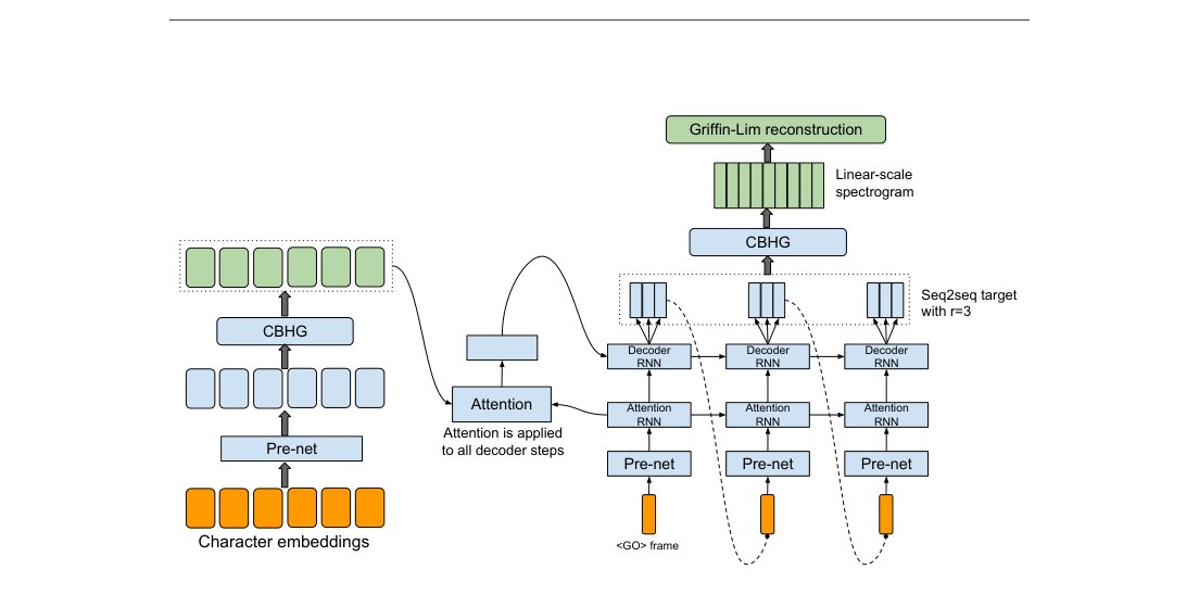
Figure 1: Model architecture. The model takes characters as input and outputs the corresponding raw spectrogram, which is then fed to the Griffin-Lim reconstruction algorithm to synthesize speech.

图 1：模型结构。模型以字符为输入，输出对应的原始频谱图，再经 Griffin-Lim 重建算法合成语音。

2 Related Work

2 相关工作

WaveNet (van den Oord et al. 2016) is a powerful generative model of audio. It works well for TTS, but is slow due to its sample-level autoregressive nature. It also requires conditioning on linguistic features from an existing TTS frontend, and thus is not end-to-end: it only replaces the vocoder and acoustic model. Another recently-developed neural model is DeepVoice (Arik et al. 2017), which replaces every component in a typical TTS pipeline by a corresponding neural network. However, each component is independently trained, and it’s nontrivial to change the system to train in an end-to-end fashion.

WaveNet（van den Oord et al. 2016）是强大的音频生成模型，用于 TTS 效果好，但按采样点自回归，速度慢；且需条件于已有 TTS 前端给出的语言学特征，因此并非端到端——它只替换了声码器与声学模型。另一较新的神经模型 DeepVoice（Arik et al. 2017）把典型 TTS 流水线中每个部件换成对应神经网络，但各部件仍独立训练，改造成端到端并不平凡。

To our knowledge, Wang et al. 2016 is the earliest work touching end-to-end TTS using seq2seq with attention. However, it requires a pre-trained hidden Markov model (HMM) aligner to help the seq2seq model learn the alignment. It’s hard to tell how much alignment is learned by the seq2seq per se. Second, a few tricks are used to get the model trained, which the authors note hurts prosody. Third, it predicts vocoder parameters hence needs a vocoder. Furthermore, the model is trained on phoneme inputs and the experimental results seem to be somewhat limited.

据我们所知，Wang et al. 2016 最早用带注意力的 seq2seq 触及端到端 TTS。但它需要预训练的隐马尔可夫模型（HMM）对齐器帮助 seq2seq 学对齐，很难说有多少对齐是 seq2seq 自己学到的。其次，为训起来用了若干技巧，作者也承认这会伤韵律。其三，预测的是声码器参数，因而仍需声码器。此外模型以音素为输入，实验规模似乎也有限。

Char2Wav (Sotelo et al. 2017) is an independently-developed end-to-end model that can be trained on characters. However, Char2Wav still predicts vocoder parameters before using a SampleRNN neural vocoder (Mehri et al. 2016), whereas Tacotron directly predicts raw spectrogram. Also, their seq2seq and SampleRNN models need to be separately pre-trained, but our model can be trained from scratch. Finally, we made several key modifications to the vanilla seq2seq paradigm. As shown later, a vanilla seq2seq model does not work well for character-level inputs.

Char2Wav（Sotelo et al. 2017）是另一独立发展的端到端模型，也可在字符上训练。但它仍先预测声码器参数，再接 SampleRNN 神经声码器（Mehri et al. 2016），而 Tacotron 直接预测原始频谱图。他们的 seq2seq 与 SampleRNN 还需分别预训练，我们的模型则可从头训练。最后，我们对朴素 seq2seq 范式做了若干关键改动；后文会看到，朴素 seq2seq 对字符级输入并不好用。

3 Model Architecture

3 模型结构

The backbone of Tacotron is a seq2seq model with attention (Bahdanau et al. 2014; Vinyals et al. 2015). Figure 1 depicts the model, which includes an encoder, an attention-based decoder, and a post-processing net. At a high-level, our model takes characters as input and produces spectrogram frames, which are then converted to waveforms. We describe these components below.

Tacotron 的主干是带注意力的 seq2seq（Bahdanau et al. 2014；Vinyals et al. 2015）。图 1 给出模型，含编码器、基于注意力的解码器与后处理网络。整体上，模型以字符为输入，产出频谱图帧，再转成波形。下面分述各部件。

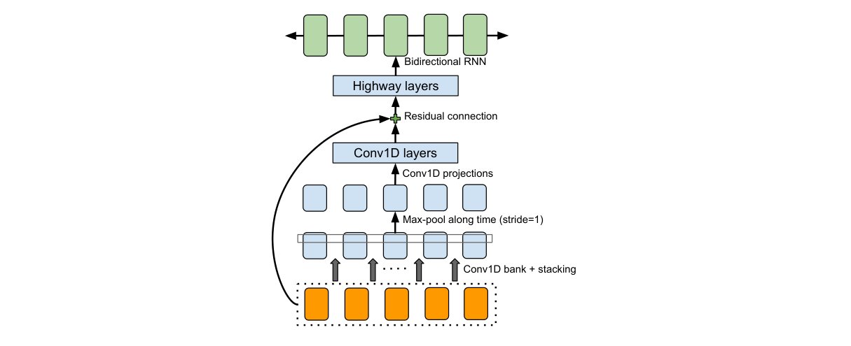
Figure 2: The CBHG (1-D convolution bank + highway network + bidirectional GRU) module adapted from Lee et al. 2016.

图 2：改编自 Lee et al. 2016 的 CBHG（一维卷积组 + 高速网络 + 双向 GRU）模块。

3.1 CBHG module

3.1 CBHG 模块

We first describe a building block dubbed CBHG, illustrated in Figure 2. CBHG consists of a bank of 1-D convolutional filters, followed by highway networks (Srivastava et al. 2015) and a bidirectional gated recurrent unit (GRU) (Chung et al. 2014) recurrent neural net (RNN). CBHG is a powerful module for extracting representations from sequences. The input sequence is first convolved with $K$ sets of 1-D convolutional filters, where the $k$-th set contains $C_{k}$ filters of width $k$ (i.e. $k=1,2,\ldots,K$). These filters explicitly model local and contextual information (akin to modeling unigrams, bigrams, up to $K$-grams). The convolution outputs are stacked together and further max pooled along time to increase local invariances. Note that we use a stride of 1 to preserve the original time resolution. We further pass the processed sequence to a few fixed-width 1-D convolutions, whose outputs are added with the original input sequence via residual connections (He et al. 2016). Batch normalization (Ioffe & Szegedy 2015) is used for all convolutional layers. The convolution outputs are fed into a multi-layer highway network to extract high-level features. Finally, we stack a bidirectional GRU RNN on top to extract sequential features from both forward and backward context. CBHG is inspired from work in machine translation (Lee et al. 2016), where the main differences from Lee et al. 2016 include using non-causal convolutions, batch normalization, residual connections, and stride=1 max pooling. We found that these modifications improved generalization.

先介绍名为 CBHG 的积木块，见图 2。CBHG 由一组一维卷积滤波器、其后的高速网络（Srivastava et al. 2015）以及双向门控循环单元（GRU）（Chung et al. 2014）RNN 组成，擅长从序列抽取表示。输入序列先与 $K$ 组一维卷积滤波器卷积，第 $k$ 组含宽度为 $k$ 的 $C_{k}$ 个滤波器（即 $k=1,2,\ldots,K$）。这些滤波器显式建模局部与上下文信息（类似一元、二元直至 $K$ 元）。卷积输出堆叠后沿时间做最大池化，以增强局部不变性；步长取 1，以保留原始时间分辨率。再经若干固定宽度一维卷积，输出通过残差连接（He et al. 2016）与原输入相加。所有卷积层使用批归一化（Ioffe & Szegedy 2015）。卷积输出送入多层高速网络抽取高层特征，顶端再叠双向 GRU，以融合前向与后向上下文。CBHG 启发自机器翻译工作（Lee et al. 2016）；与 Lee et al. 2016 的主要差别包括：非因果卷积、批归一化、残差连接，以及 stride=1 的最大池化。我们发现这些改动提升了泛化。

3.2 Encoder

3.2 编码器

The goal of the encoder is to extract robust sequential representations of text. The input to the encoder is a character sequence, where each character is represented as a one-hot vector and embedded into a continuous vector. We then apply a set of non-linear transformations, collectively called a “pre-net”, to each embedding. We use a bottleneck layer with dropout as the pre-net in this work, which helps convergence and improves generalization. A CBHG module transforms the pre-net outputs into the final encoder representation used by the attention module. We found that this CBHG-based encoder not only reduces overfitting, but also makes fewer mispronunciations than a standard multi-layer RNN encoder (see our linked page of audio samples).

编码器的目标是抽取稳健的文本序列表示。输入为字符序列：每字符表示为 one-hot，再嵌入连续向量。随后对每个嵌入施加一组非线性变换，统称「pre-net」。本文用带 dropout 的瓶颈层作 pre-net，有助于收敛与泛化。CBHG 模块把 pre-net 输出变成注意力模块所用的最终编码器表示。我们发现基于 CBHG 的编码器不仅减轻过拟合，误读也少于标准多层 RNN 编码器（见链接页上的音频样例）。

3.3 Decoder

3.3 解码器

We use a content-based tanh attention decoder (see e.g. Vinyals et al. 2015), where a stateful recurrent layer produces the attention query at each decoder time step. We concatenate the context vector and the attention RNN cell output to form the input to the decoder RNNs. We use a stack of GRUs with vertical residual connections (Wu et al. 2016) for the decoder. We found the residual connections speed up convergence. The decoder target is an important design choice. While we could directly predict raw spectrogram, it’s a highly redundant representation for the purpose of learning alignment between speech signal and text (which is really the motivation of using seq2seq for this task). Because of this redundancy, we use a different target for seq2seq decoding and waveform synthesis. The seq2seq target can be highly compressed as long as it provides sufficient intelligibility and prosody information for an inversion process, which could be fixed or trained. We use 80-band mel-scale spectrogram as the target, though fewer bands or more concise targets such as cepstrum could be used. We use a post-processing network (discussed below) to convert from the seq2seq target to waveform.

我们采用基于内容的 tanh 注意力解码器（参见 Vinyals et al. 2015）：有状态循环层在每个解码时间步产生注意力查询。将上下文向量与注意力 RNN 单元输出拼接，作为解码器 RNN 的输入。解码器用带纵向残差连接的 GRU 堆叠（Wu et al. 2016）；残差加快收敛。解码目标是重要设计选择。虽可直接预测原始频谱图，但对学习语音与文本对齐（这正是用 seq2seq 做本任务的动机）而言，该表示高度冗余。因此我们为 seq2seq 解码与波形合成使用不同目标：只要能为（固定或可训的）反演提供足够可懂度与韵律信息，seq2seq 目标就可高度压缩。我们采用 80 带梅尔频谱作为目标，也可用更少频带或倒谱等更紧凑目标。再用后处理网络（见下）把 seq2seq 目标转成波形所需表示。

Spectral analysis	pre-emphasis: 0.97; frame length: 50 ms;
	frame shift: 12.5 ms; window type: Hann
Character embedding	256-D
Encoder CBHG	Conv1D bank: $K$=16, conv-$k$-128-ReLU
	Max pooling: stride=1, width=2
	Conv1D projections: conv-3-128-ReLU
	$\rightarrow$ conv-3-128-Linear
	Highway net: 4 layers of FC-128-ReLU
	Bidirectional GRU: 128 cells
Encoder pre-net	FC-256-ReLU $\rightarrow$ Dropout(0.5) $\rightarrow$
	FC-128-ReLU $\rightarrow$ Dropout(0.5)
Decoder pre-net	FC-256-ReLU $\rightarrow$ Dropout(0.5)$\rightarrow$
	FC-128-ReLU $\rightarrow$ Dropout(0.5)
Decoder RNN	2-layer residual GRU (256 cells)
Attention RNN	1-layer GRU (256 cells)
Post-processing net	Conv1D bank: $K$=8, conv-k-128-ReLU
CBHG	Max pooling: stride=1, width=2
	Conv1D projections: conv-3-256-ReLU
	$\rightarrow$ conv-3-80-Linear
	Highway net: 4 layers of FC-128-ReLU
	Bidirectional GRU: 128 cells
Reduction factor ($r$)	2

Table 1: Hyper-parameters and network architectures. “conv-$k$-$c$-ReLU” denotes 1-D convolution with width $k$ and $c$ output channels with ReLU activation. FC stands for fully-connected.

频谱分析	预加重：0.97；帧长：50 ms；
	帧移：12.5 ms；窗型：Hann
字符嵌入	256 维
编码器 CBHG	Conv1D 组：$K$=16，conv-$k$-128-ReLU
	最大池化：stride=1，width=2
	Conv1D 投影：conv-3-128-ReLU
	$\rightarrow$ conv-3-128-Linear
	高速网络：4 层 FC-128-ReLU
	双向 GRU：128 单元
编码器 pre-net	FC-256-ReLU $\rightarrow$ Dropout(0.5) $\rightarrow$
	FC-128-ReLU $\rightarrow$ Dropout(0.5)
解码器 pre-net	FC-256-ReLU $\rightarrow$ Dropout(0.5)$\rightarrow$
	FC-128-ReLU $\rightarrow$ Dropout(0.5)
解码器 RNN	2 层残差 GRU（256 单元）
注意力 RNN	1 层 GRU（256 单元）
后处理网络	Conv1D 组：$K$=8，conv-k-128-ReLU
CBHG	最大池化：stride=1，width=2
	Conv1D 投影：conv-3-256-ReLU
	$\rightarrow$ conv-3-80-Linear
	高速网络：4 层 FC-128-ReLU
	双向 GRU：128 单元
缩减因子（$r$）	2

表 1：超参数与网络结构。「conv-$k$-$c$-ReLU」表示宽度 $k$、输出通道 $c$、ReLU 激活的一维卷积。FC 为全连接。

We use a simple fully-connected output layer to predict the decoder targets. An important trick we discovered was predicting multiple, non-overlapping output frames at each decoder step. Predicting $r$ frames at once divides the total number of decoder steps by $r$, which reduces model size, training time, and inference time. More importantly, we found this trick to substantially increase convergence speed, as measured by a much faster (and more stable) alignment learned from attention. This is likely because neighboring speech frames are correlated and each character usually corresponds to multiple frames. Emitting one frame at a time forces the model to attend to the same input token for multiple timesteps; emitting multiple frames allows the attention to move forward early in training. A similar trick is also used in Zen et al. 2016 but mainly to speed up inference.

我们用简单的全连接输出层预测解码目标。一个重要技巧是：每步预测多个互不重叠的输出帧。一次预测 $r$ 帧，把总解码步数除以 $r$，从而减小模型、缩短训练与推理时间。更重要的是，按注意力所学对齐的速度与稳定性衡量，该技巧显著加快收敛。原因可能是邻近语音帧相关，且每个字符通常对应多帧：一次只发一帧会迫使模型对同一输入 token 保持多步注意力；一次发多帧则让注意力在训练早期就能前移。Zen et al. 2016 也用过类似技巧，但主要是为加速推理。

The first decoder step is conditioned on an all-zero frame, which represents a $<$GO$>$ frame. In inference, at decoder step $t$, the last frame of the $r$ predictions is fed as input to the decoder at step $t+1$. Note that feeding the last prediction is an ad-hoc choice here – we could use all $r$ predictions. During training, we always feed every $r$-th ground truth frame to the decoder. The input frame is passed to a pre-net as is done in the encoder. Since we do not use techniques such as scheduled sampling (Bengio et al. 2015) (we found it to hurt audio quality), the dropout in the pre-net is critical for the model to generalize, as it provides a noise source to resolve the multiple modalities in the output distribution.

解码第一步条件于全零帧，表示 $<$GO$>$ 帧。推理时，第 $t$ 步的 $r$ 个预测中取最后一帧，作为第 $t+1$ 步解码器输入——这是特设选择，也可用全部 $r$ 个预测。训练时始终把每第 $r$ 个真值帧喂给解码器。输入帧同样经 pre-net。我们未用 scheduled sampling（Bengio et al. 2015）（发现会伤音质），因此 pre-net 中的 dropout 对泛化至关重要：它提供噪声源，以化解输出分布的多模态。

3.4 Post-processing net and waveform synthesis

3.4 后处理网络与波形合成

As mentioned above, the post-processing net’s task is to convert the seq2seq target to a target that can be synthesized into waveforms. Since we use Griffin-Lim as the synthesizer, the post-processing net learns to predict spectral magnitude sampled on a linear-frequency scale. Another motivation of the post-processing net is that it can see the full decoded sequence. In contrast to seq2seq, which always runs from left to right, it has both forward and backward information to correct the prediction error for each individual frame. In this work, we use a CBHG module for the post-processing net, though a simpler architecture likely works as well. The concept of a post-processing network is highly general. It could be used to predict alternative targets such as vocoder parameters, or as a WaveNet-like neural vocoder (van den Oord et al. 2016; Mehri et al. 2016; Arik et al. 2017) that synthesizes waveform samples directly.

如上所述，后处理网络把 seq2seq 目标转成可合成波形的目标。因声码器选用 Griffin-Lim，后处理网络学习预测线性频率尺度上的频谱幅度。另一动机是：后处理网络能看到完整解码序列；相对总是从左到右的 seq2seq，它同时有前向与后向信息，可纠正各帧预测误差。本文用 CBHG 作后处理网络，更简单结构多半也行。后处理网络概念很泛：既可预测声码器参数等替代目标，也可做成类似 WaveNet 的神经声码器（van den Oord et al. 2016；Mehri et al. 2016；Arik et al. 2017）直接合成波形采样点。

We use the Griffin-Lim algorithm (Griffin & Lim 1984) to synthesize waveform from the predicted spectrogram. We found that raising the predicted magnitudes by a power of 1.2 before feeding to Griffin-Lim reduces artifacts, likely due to its harmonic enhancement effect. We observed that Griffin-Lim converges after 50 iterations (in fact, about 30 iterations seems to be enough), which is reasonably fast. We implemented Griffin-Lim in TensorFlow (Abadi et al. 2016) hence it’s also part of the model. While Griffin-Lim is differentiable (it does not have trainable weights), we do not impose any loss on it in this work. We emphasize that our choice of Griffin-Lim is for simplicity; while it already yields strong results, developing a fast and high-quality trainable spectrogram to waveform inverter is ongoing work.

我们用 Griffin-Lim 算法（Griffin & Lim 1984）从预测频谱合成波形。发现把预测幅度升到 1.2 次幂再送入 Griffin-Lim 可减少伪影，可能因其谐波增强效应。Griffin-Lim 约 50 次迭代即收敛（约 30 次似乎也够），速度尚可。我们在 TensorFlow（Abadi et al. 2016）中实现 Griffin-Lim，因而也是模型一部分。虽可微分（无可训权重），本文未对其施加损失。强调选用 Griffin-Lim 是为简单；它已能给出强结果，但快速高质量、可训练的频谱到波形反演仍在推进。

4 Model Details

4 模型细节

Table 1 lists the hyper-parameters and network architectures. We use log magnitude spectrogram with Hann windowing, 50 ms frame length, 12.5 ms frame shift, and 2048-point Fourier transform. We also found pre-emphasis (0.97) to be helpful. We use 24 kHz sampling rate for all experiments.

表 1 列出超参数与网络结构。我们用对数幅度频谱，Hann 窗，帧长 50 ms，帧移 12.5 ms，2048 点傅里叶变换；并发现预加重（0.97）有帮助。全部实验采样率 24 kHz。

We use $r$ = 2 (output layer reduction factor) for the MOS results in this paper, though larger $r$ values (e.g. $r$ = 5) also work well. We use the Adam optimizer (Kingma & Ba 2015) with learning rate decay, which starts from 0.001 and is reduced to 0.0005, 0.0003, and 0.0001 after 500K, 1M and 2M global steps, respectively. We use a simple $\ell$1 loss for both seq2seq decoder (mel-scale spectrogram) and post-processing net (linear-scale spectrogram). The two losses have equal weights.

本文 MOS 结果用 $r$ = 2（输出层缩减因子），更大的 $r$（如 $r$ = 5）也工作良好。优化器用 Adam（Kingma & Ba 2015）并衰减学习率：从 0.001 起，在全局步 500K、1M、2M 后分别降到 0.0005、0.0003、0.0001。seq2seq 解码器（梅尔频谱）与后处理网络（线性频谱）均用简单 $\ell$1 损失，两损失等权。

We train using a batch size of 32, where all sequences are padded to a max length. It’s a common practice to train sequence models with a loss mask, which masks loss on zero-padded frames. However, we found that models trained this way don’t know when to stop emitting outputs, causing repeated sounds towards the end. One simple trick to get around this problem is to also reconstruct the zero-padded frames.

训练 batch size 为 32，序列均填充到最大长度。序列模型常见做法是用损失掩码忽略零填充帧上的损失。但我们发现如此训练的模型不知道何时停止输出，末尾会反复出声。一个简单对策是：同样重建零填充帧。

5 Experiments

5 实验

We train Tacotron on an internal North American English dataset, which contains about 24.6 hours of speech data spoken by a professional female speaker. The phrases are text normalized, e.g. “16” is converted to “sixteen”.

我们在内部北美英语数据集上训练 Tacotron，约 24.6 小时，由一名专业女声录制。短语做过文本规范化，例如「16」转为「sixteen」。

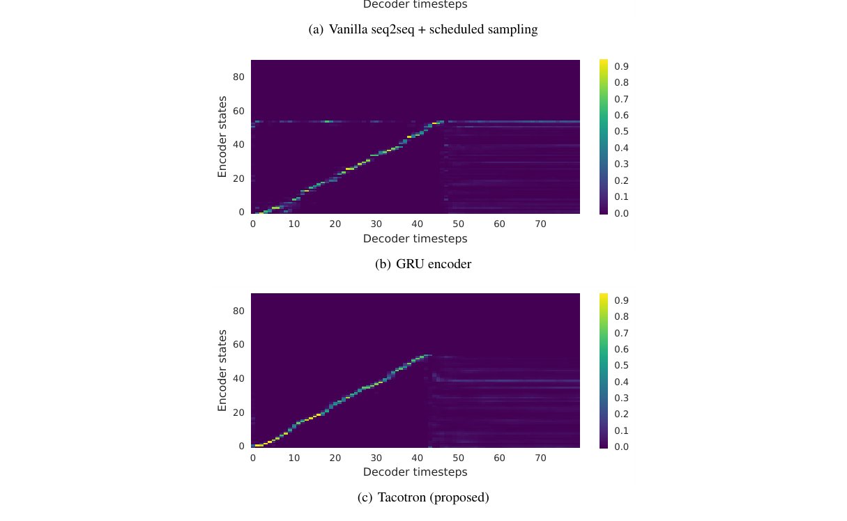
(a) Vanilla seq2seq + scheduled sampling

（a）朴素 seq2seq + scheduled sampling

5.1 Ablation analysis

5.1 消融分析

We conduct a few ablation studies to understand the key components in our model. As is common for generative models, it’s hard to compare models based on objective metrics, which often do not correlate well with perception (Theis et al. 2015). We mainly rely on visual comparisons instead. We strongly encourage readers to listen to the provided samples.

我们做若干消融，以理解模型关键部件。生成模型常见情况是：客观指标往往与感知相关不强，难以据此比较（Theis et al. 2015）。我们主要依赖可视化对比，并强烈建议读者听提供的样例。

First, we compare with a vanilla seq2seq model. Both the encoder and decoder use 2 layers of residual RNNs, where each layer has 256 GRU cells (we tried LSTM and got similar results). No pre-net or post-processing net is used, and the decoder directly predicts linear-scale log magnitude spectrogram. We found that scheduled sampling (sampling rate 0.5) is required for this model to learn alignments and generalize. We show the learned attention alignment in Figure 3. Figure 3(a) reveals that the vanilla seq2seq learns a poor alignment. One problem is that attention tends to get stuck for many frames before moving forward, which causes bad speech intelligibility in the synthesized signal. The naturalness and overall duration are destroyed as a result. In contrast, our model learns a clean and smooth alignment, as shown in Figure 3(c).

首先与朴素 seq2seq 比较。编码器与解码器均为 2 层残差 RNN，每层 256 个 GRU 单元（试过 LSTM，结果类似）。不用 pre-net 与后处理网络，解码器直接预测线性尺度对数幅度频谱。发现该模型需要 scheduled sampling（采样率 0.5）才能学对齐并泛化。学到的注意力对齐见图 3。图 3(a) 显示朴素 seq2seq 对齐很差：注意力常卡住许多帧才前移，合成信号可懂度差，自然度与总体时长也被破坏。相比之下，我们的模型学到干净平滑的对齐，见图 3(c)。

Second, we compare with a model with the CBHG encoder replaced by a 2-layer residual GRU encoder. The rest of the model, including the encoder pre-net, remain exactly the same. Comparing Figure 3(b) and 3(c), we can see that the alignment from the GRU encoder is noisier. Listening to synthesized signals, we found that noisy alignment often leads to mispronunciations. The CBHG encoder reduces overfitting and generalizes well to long and complex phrases.

其次，把 CBHG 编码器换成 2 层残差 GRU 编码器，其余（含编码器 pre-net）不变。对比图 3(b) 与 3(c)，GRU 编码器的对齐更嘈杂。听合成信号可见，嘈杂对齐常导致误读。CBHG 编码器减轻过拟合，对长而复杂的短语泛化更好。

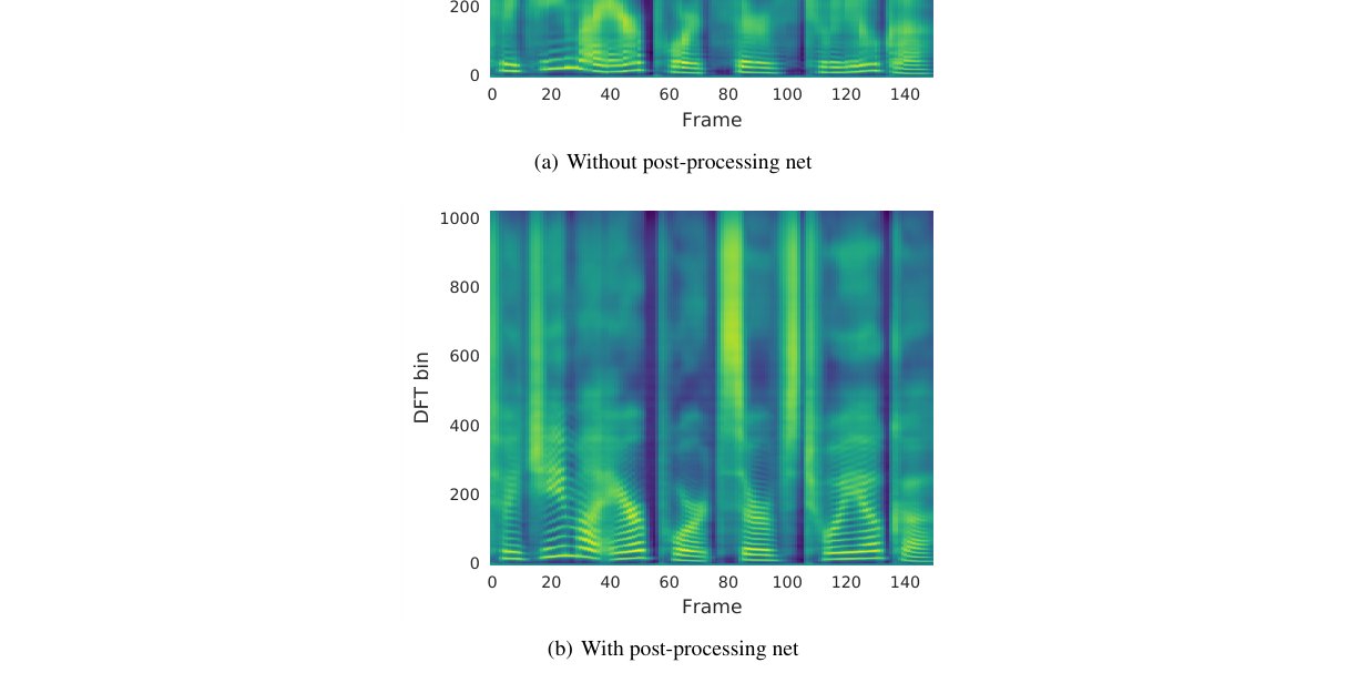
(a) Without post-processing net

（a）无后处理网络

Figures 4(a) and 4(b) demonstrate the benefit of using the post-processing net. We trained a model without the post-processing net while keeping all the other components untouched (except that the decoder RNN predicts linear-scale spectrogram). With more contextual information, the prediction from the post-processing net contains better resolved harmonics (e.g. higher harmonics between bins 100 and 400) and high frequency formant structure, which reduces synthesis artifacts.

图 4(a) 与 4(b) 展示使用后处理网络的收益。我们去掉后处理网络、其余不变（解码器 RNN 改为预测线性频谱）训练对照。有了更多上下文，后处理网络的预测谐波分辨更好（例如 bin 100–400 之间更高次谐波），高频共振峰结构也更清晰，从而减少合成伪影。

5.2 Mean opinion score tests

5.2 平均意见分测试

We conduct mean opinion score tests, where the subjects were asked to rate the naturalness of the stimuli in a 5-point Likert scale score. The MOS tests were crowdsourced from native speakers. 100 unseen phrases were used for the tests and each phrase received 8 ratings. When computing MOS, we only include ratings where headphones were used. We compare our model with a parametric (based on LSTM (Zen et al. 2016)) and a concatenative system (Gonzalvo et al. 2016), both of which are in production. As shown in Table 2, Tacotron achieves an MOS of 3.82, which outperforms the parametric system. Given the strong baselines and the artifacts introduced by the Griffin-Lim synthesis, this represents a very promising result.

我们做平均意见分测试：受试者按 5 点李克特量表给刺激的自然度打分。MOS 由母语者众包；用 100 条未见短语，每条 8 次评分。计算 MOS 时只保留使用耳机的评分。对照为量产中的参数系统（基于 LSTM，Zen et al. 2016）与拼接系统（Gonzalvo et al. 2016）。如表 2，Tacotron 取得 MOS 3.82，超过参数系统。基线很强，且 Griffin-Lim 会引入伪影，这一结果仍很有前景。

	mean opinion score
Tacotron	3.82 $\pm$ 0.085
Parametric	3.69 $\pm$ 0.109
Concatenative	4.09 $\pm$ 0.119

Table 2: 5-scale mean opinion score evaluation.

	平均意见分
Tacotron	3.82 $\pm$ 0.085
参数系统	3.69 $\pm$ 0.109
拼接系统	4.09 $\pm$ 0.119

表 2：5 分制平均意见分评测。

6 Discussions

6 讨论

We have proposed Tacotron, an integrated end-to-end generative TTS model that takes a character sequence as input and outputs the corresponding spectrogram. With a very simple waveform synthesis module, it achieves a 3.82 MOS score on US English, outperforming a production parametric system in terms of naturalness. Tacotron is frame-based, so the inference is substantially faster than sample-level autoregressive methods. Unlike previous work, Tacotron does not need hand-engineered linguistic features or complex components such as an HMM aligner. It can be trained from scratch with random initialization. We perform simple text normalization, though recent advancements in learned text normalization (Sproat & Jaitly 2016) may render this unnecessary in the future.

我们提出 Tacotron：一体化端到端生成式 TTS，以字符序列为输入、输出对应频谱图。配合极简波形合成模块，在美式英语上 MOS 达 3.82，自然度超过量产参数系统。Tacotron 按帧生成，推理明显快于按采样点自回归的方法。与先前工作不同，Tacotron 不需手工语言学特征或 HMM 对齐器等复杂部件，可从随机初始化从头训练。我们做了简单文本规范化；近年可学习文本规范化（Sproat & Jaitly 2016）的进展，未来或许能使这一步也不再必要。

We have yet to investigate many aspects of our model; many early design decisions have gone unchanged. Our output layer, attention module, loss function, and Griffin-Lim-based waveform synthesizer are all ripe for improvement. For example, it’s well known that Griffin-Lim outputs may have audible artifacts. We are currently working on fast and high-quality neural-network-based spectrogram inversion.

模型许多方面尚未细究，早期设计选择也多未改动。输出层、注意力、损失函数，以及基于 Griffin-Lim 的波形合成都有改进空间。例如 Griffin-Lim 输出常有可闻伪影。我们正推进快速高质量的神经网络频谱反演。

Acknowledgments

The authors would like to thank Heiga Zen and Ziang Xie for constructive discussions and feedback.

致谢

作者感谢 Heiga Zen 与 Ziang Xie 的建设性讨论与反馈。

References

参考文献

Abadi et al. (2016) Martín Abadi, Ashish Agarwal, Paul Barham, Eugene Brevdo, Zhifeng Chen, Craig Citro, Greg S Corrado, Andy Davis, Jeffrey Dean, Matthieu Devin, et al. TensorFlow: Large-scale machine learning on heterogeneous distributed systems. arXiv preprint arXiv:1603.04467 , 2016.

Agiomyrgiannakis (2015) Yannis Agiomyrgiannakis. Vocaine the vocoder and applications in speech synthesis. In Acoustics, Speech and Signal Processing (ICASSP), 2015 IEEE International Conference on , pp. 4230–4234. IEEE, 2015.

Arik et al. (2017) Sercan Arik, Mike Chrzanowski, Adam Coates, Gregory Diamos, Andrew Gibiansky, Yongguo Kang, Xian Li, John Miller, Jonathan Raiman, Shubho Sengupta, and Mohammad Shoeybi. Deep voice: Real-time neural text-to-speech. arXiv preprint arXiv:1702.07825 , 2017.

Bahdanau et al. (2014) Dzmitry Bahdanau, Kyunghyun Cho, and Yoshua Bengio. Neural machine translation by jointly learning to align and translate. arXiv preprint arXiv:1409.0473 , 2014.

Bengio et al. (2015) Samy Bengio, Oriol Vinyals, Navdeep Jaitly, and Noam Shazeer. Scheduled sampling for sequence prediction with recurrent neural networks. In Advances in Neural Information Processing Systems , pp. 1171–1179, 2015.

Chan et al. (2016) William Chan, Navdeep Jaitly, Quoc Le, and Oriol Vinyals. Listen, attend and spell: A neural network for large vocabulary conversational speech recognition. In Acoustics, Speech and Signal Processing (ICASSP), 2016 IEEE International Conference on , pp. 4960–4964. IEEE, 2016.

Chung et al. (2014) Junyoung Chung, Caglar Gulcehre, KyungHyun Cho, and Yoshua Bengio. Empirical evaluation of gated recurrent neural networks on sequence modeling. arXiv preprint arXiv:1412.3555 , 2014.

Gonzalvo et al. (2016) Xavi Gonzalvo, Siamak Tazari, Chun-an Chan, Markus Becker, Alexander Gutkin, and Hanna Silen. Recent advances in Google real-time HMM-driven unit selection synthesizer. In Proc. Interspeech , pp. 2238–2242, 2016.

Griffin & Lim (1984) Daniel Griffin and Jae Lim. Signal estimation from modified short-time fourier transform. IEEE Transactions on Acoustics, Speech, and Signal Processing , 32(2):236–243, 1984.

He et al. (2016) Kaiming He, Xiangyu Zhang, Shaoqing Ren, and Jian Sun. Deep residual learning for image recognition. In Proceedings of the IEEE Conference on Computer Vision and Pattern Recognition , pp. 770–778, 2016.

Ioffe & Szegedy (2015) Sergey Ioffe and Christian Szegedy. Batch normalization: Accelerating deep network training by reducing internal covariate shift. arXiv preprint arXiv:1502.03167 , 2015.

Kingma & Ba (2015) Diederik Kingma and Jimmy Ba. Adam: A method for stochastic optimization. Proceedings of the 3rd International Conference on Learning Representations (ICLR) , 2015.

Lee et al. (2016) Jason Lee, Kyunghyun Cho, and Thomas Hofmann. Fully character-level neural machine translation without explicit segmentation. arXiv preprint arXiv:1610.03017 , 2016.

Mehri et al. (2016) Soroush Mehri, Kundan Kumar, Ishaan Gulrajani, Rithesh Kumar, Shubham Jain, Jose Sotelo, Aaron Courville, and Yoshua Bengio. SampleRNN: An unconditional end-to-end neural audio generation model. arXiv preprint arXiv:1612.07837 , 2016.

Sotelo et al. (2017) Jose Sotelo, Soroush Mehri, Kundan Kumar, João Felipe Santos, Kyle Kastner, Aaron Courville, and Yoshua Bengio. Char2Wav: End-to-end speech synthesis. In ICLR2017 workshop submission , 2017.

Sproat & Jaitly (2016) Richard Sproat and Navdeep Jaitly. RNN approaches to text normalization: A challenge. arXiv preprint arXiv:1611.00068 , 2016.

Srivastava et al. (2015) Rupesh Kumar Srivastava, Klaus Greff, and Jürgen Schmidhuber. Highway networks. arXiv preprint arXiv:1505.00387 , 2015.

Sutskever et al. (2014) Ilya Sutskever, Oriol Vinyals, and Quoc V Le. Sequence to sequence learning with neural networks. In Advances in neural information processing systems , pp. 3104–3112, 2014.

Taylor (2009) Paul Taylor. Text-to-speech synthesis . Cambridge university press, 2009.

Theis et al. (2015) Lucas Theis, Aäron van den Oord, and Matthias Bethge. A note on the evaluation of generative models. arXiv preprint arXiv:1511.01844 , 2015.

van den Oord et al. (2016) Aäron van den Oord, Sander Dieleman, Heiga Zen, Karen Simonyan, Oriol Vinyals, Alex Graves, Nal Kalchbrenner, Andrew Senior, and Koray Kavukcuoglu. WaveNet: A generative model for raw audio. arXiv preprint arXiv:1609.03499 , 2016.

Vinyals et al. (2015) Oriol Vinyals, Łukasz Kaiser, Terry Koo, Slav Petrov, Ilya Sutskever, and Geoffrey Hinton. Grammar as a foreign language. In Advances in Neural Information Processing Systems , pp. 2773–2781, 2015.

Wang et al. (2016) Wenfu Wang, Shuang Xu, and Bo Xu. First step towards end-to-end parametric TTS synthesis: Generating spectral parameters with neural attention. In Proceedings Interspeech , pp. 2243–2247, 2016.

Wu et al. (2016) Yonghui Wu, Mike Schuster, Zhifeng Chen, Quoc V Le, Mohammad Norouzi, Wolfgang Macherey, Maxim Krikun, Yuan Cao, Qin Gao, Klaus Macherey, et al. Google’s neural machine translation system: Bridging the gap between human and machine translation. arXiv preprint arXiv:1609.08144 , 2016.

Zen et al. (2009) Heiga Zen, Keiichi Tokuda, and Alan W Black. Statistical parametric speech synthesis. Speech Communication , 51(11):1039–1064, 2009.

Zen et al. (2016) Heiga Zen, Yannis Agiomyrgiannakis, Niels Egberts, Fergus Henderson, and Przemysław Szczepaniak. Fast, compact, and high quality LSTM-RNN based statistical parametric speech synthesizers for mobile devices. Proceedings Interspeech , 2016.