Exploring the Limits of Transfer Learning with a Unified Text-to-Text Transformer
Colin Raffel, Noam Shazeer, Adam Roberts, Katherine Lee, Sharan Narang, Michael Matena, Yanqi Zhou, Wei Li, and Peter J. Liu
Colin Raffel、Noam Shazeer、Adam Roberts、Katherine Lee、Sharan Narang、Michael Matena、Yanqi Zhou、Wei Li、Peter J. Liu
Exploring the Limits of Transfer Learning with a Unified Text-to-Text Transformer
用统一的文本到文本 Transformer 探索迁移学习的极限(Exploring the Limits of Transfer Learning with a Unified Text-to-Text Transformer)
Colin Raffel craffel@gmail.com Thanks: Equal contribution. A description of each author’s contribution is available in Appendix A . Correspondence to craffel@gmail.com . Noam Shazeer noam@google.com Adam Roberts adarob@google.com Katherine Lee katherinelee@google.comSharan Narang sharannarang@google.comMichael Matena mmatena@google.comYanqi Zhou yanqiz@google.comWei Li mweili@google.comPeter J. Liu peterjliu@google.comGoogle, Mountain View, CA 94043, USA
Colin Raffel craffel@gmail.com Noam Shazeer Adam Roberts Katherine Lee Sharan Narang Michael Matena Yanqi Zhou Wei Li Peter J. Liu
Google
作者贡献说明见附录 A;通信请致 craffel@gmail.com
Abstract
摘要
Transfer learning, where a model is first pre-trained on a data-rich task before being fine-tuned on a downstream task, has emerged as a powerful technique in natural language processing (NLP). The effectiveness of transfer learning has given rise to a diversity of approaches, methodology, and practice. In this paper, we explore the landscape of transfer learning techniques for NLP by introducing a unified framework that converts all text-based language problems into a text-to-text format. Our systematic study compares pre-training objectives, architectures, unlabeled data sets, transfer approaches, and other factors on dozens of language understanding tasks. By combining the insights from our exploration with scale and our new ‘‘Colossal Clean Crawled Corpus’’, we achieve state-of-the-art results on many benchmarks covering summarization, question answering, text classification, and more. To facilitate future work on transfer learning for NLP, we release our data set, pre-trained models, and code.[^1]
迁移学习——先在数据丰富的任务上预训练,再在下游任务上微调——已成为自然语言处理(NLP)中的有力技术。迁移学习的有效性催生了多样的方法与实践。本文引入统一框架,把所有基于文本的语言问题都转成文本到文本(text-to-text)格式,借此系统梳理 NLP 迁移学习的版图。我们在数十个语言理解任务上比较预训练目标、架构、无标注数据集、迁移方式及其他因素。把探索所得洞见与规模以及新的「超大规模清洁爬取语料」(Colossal Clean Crawled Corpus,C4)结合起来,我们在摘要、问答、文本分类等多项基准上达到当时最优。为方便后续工作,我们公开数据集、预训练模型与代码。
1 Introduction
1 引言
keywords
Training a machine learning model to perform natural language processing (NLP) tasks often requires that the model can process text in a way that is amenable to downstream learning. This can be loosely viewed as developing general-purpose knowledge that allows the model to “understand” text. This knowledge can range from low-level (e.g. the spelling or meaning of words) to high-level (e.g. that a tuba is too large to fit in most backpacks). In modern machine learning practice, providing this knowledge is rarely done explicitly; instead, it is often learned as part of an auxiliary task. For example, a historically common approach is to use word vectors (Mikolov et al. 2013b; Mikolov et al. 2013a; Pennington et al. 2014) to map word identities to a continuous representation where, ideally, similar words map to similar vectors. These vectors are often learned through an objective that, for example, encourages co-occurring words to be positioned nearby in the continuous space (Mikolov et al. 2013b).
关键词
训练机器学习模型来完成自然语言处理(NLP)任务往往要求模型能够以适合下游学习的方式处理文本. 这可被松散地视为发展通用知识,使模型能够“理解”案文。 这种知识可以从低层次(如词的拼写或意思)到高层次(如大管太大,无法融入大多数背包). 在现代机器学习实践中,提供这种知识很少被明确做到;相反,它常常被作为辅助任务的一部分来学习. 例如,一个历史上常见的方法是使用单词矢量(Mikolov等人,2013年b;Mikolov等人,2013年a;Pennington等人,2014年)将单词身份映射到一个连续的表示,理想的情况是将类似单词映射到类似矢量的地方. 这些矢量通常是通过一个目标来学习的,例如,这个目标鼓励在连续空间中共同使用词语的位置(Mikolov等人,2013年b)。
Recently, it has become increasingly common to pre-train the entire model on a data-rich task. Ideally, this pre-training causes the model to develop general-purpose abilities and knowledge that can then be transferred to downstream tasks. In applications of transfer learning to computer vision (Oquab et al. 2014; Jia et al. 2014; Huh et al. 2016; Yosinski et al. 2014), pre-training is typically done via supervised learning on a large labeled data set like ImageNet (Russakovsky et al. 2015; Deng et al. 2009). In contrast, modern techniques for transfer learning in NLP often pre-train using unsupervised learning on unlabeled data. This approach has recently been used to obtain state-of-the-art results in many of the most common NLP benchmarks (Devlin et al. 2018; Yang et al. 2019; Dong et al. 2019; Liu et al. 2019c; Lan et al. 2019). Beyond its empirical strength, unsupervised pre-training for NLP is particularly attractive because unlabeled text data is available en masse thanks to the Internet---for example, the Common Crawl project[^2] produces about 20TB of text data extracted from web pages each month. This is a natural fit for neural networks, which have been shown to exhibit remarkable scalability, i.e. it is often possible to achieve better performance simply by training a larger model on a larger data set (Hestness et al. 2017; Shazeer et al. 2017; Jozefowicz et al. 2016; Mahajan et al. 2018; Radford et al. 2019; Shazeer et al. 2018; Huang et al. 2018b; Keskar et al. 2019a).
最近,在数据丰富的任务上预先培训整个模型已变得越来越普遍。 理想的情况是,这种预训导致模式发展通用能力和知识,然后可以转移到下游任务. 在计算机视觉转移学习应用方面(Oquab等人,2014年;Jia等人,2014年;Huh等人,2016年;Yosinski等人,2014年),培训前通常通过在ImageNet(Russakovsky等人,2015年;Deng等人,2009年)等大型标注数据集的监督下学习进行。 相比之下,NLP中现代的转移学习技术往往使用无标签数据上的无监督学习进行预训. 这种方法最近被用于获得许多最常见的NLP基准的最新结果(Devlin等人,2018年;杨等人,2019年;董等人,2019年;刘等人,2019年c;兰等人,2019年). 除了经验力量之外,无监督的NLP预训特别有吸引力,因为由于互联网,无标签的文本数据可以大量获取——例如,共同爬行项目[^2]每月从网页中提取大约20TB的文本数据. 这自然适合神经网络,已经证明神经网络表现出显著的可伸缩性,即只要在更大的数据集上培训一个更大的模型,就往往有可能取得更好的性能(Hestness等人,2017年;Shazeer等人,2017年;Jozefowicz等人,2016年;Mahajan等人,2018年;Radford等人,2019年;Shazeer等人,2018年;Huang等人,2018年b;Keskar等人,2019年a).
This synergy has resulted in a great deal of recent work developing transfer learning methodology for NLP, which has produced a wide landscape of pre-training objectives (Howard and Ruder 2018; Devlin et al. 2018; Yang et al. 2019; Dong et al. 2019), unlabeled data sets (Yang et al. 2019; Liu et al. 2019c; Zellers et al. 2019), benchmarks (Wang et al. 2019b; Wang et al. 2018; Conneau and Kiela 2018), fine-tuning methods (Howard and Ruder 2018; Houlsby et al. 2019; Peters et al. 2019), and more. The rapid rate of progress and diversity of techniques in this burgeoning field can make it difficult to compare different algorithms, tease apart the effects of new contributions, and understand the space of existing methods for transfer learning. Motivated by a need for more rigorous understanding, we leverage a unified approach to transfer learning that allows us to systematically study different approaches and push the current limits of the field.
这一协同关系导致近期为NLP制定大量转移学习方法,产生了广泛的培训前目标(Howard和Ruder 2018;Devlin等人2018;Yang等人2019;Dong等人2019),未贴标签的数据集(Yang等人2019;Liu等人2019c;Zellers等人2019),基准(Wang等人2019b;Wang等人2018;Conneau和Kiela2018),微调方法(Howard和Ruder2018;Houlsby等人2019;Peters等人2019),等等. 在这个蓬勃发展的领域中技术的迅速进步和多样化,可能使得难以比较不同的算法,嘲笑新贡献的影响,并理解现有转学方法的空间. 由于需要更严格的理解,我们利用一种统一的方法来转移学习,使我们能够系统地研究不同的方法,并推进该领域目前的极限。
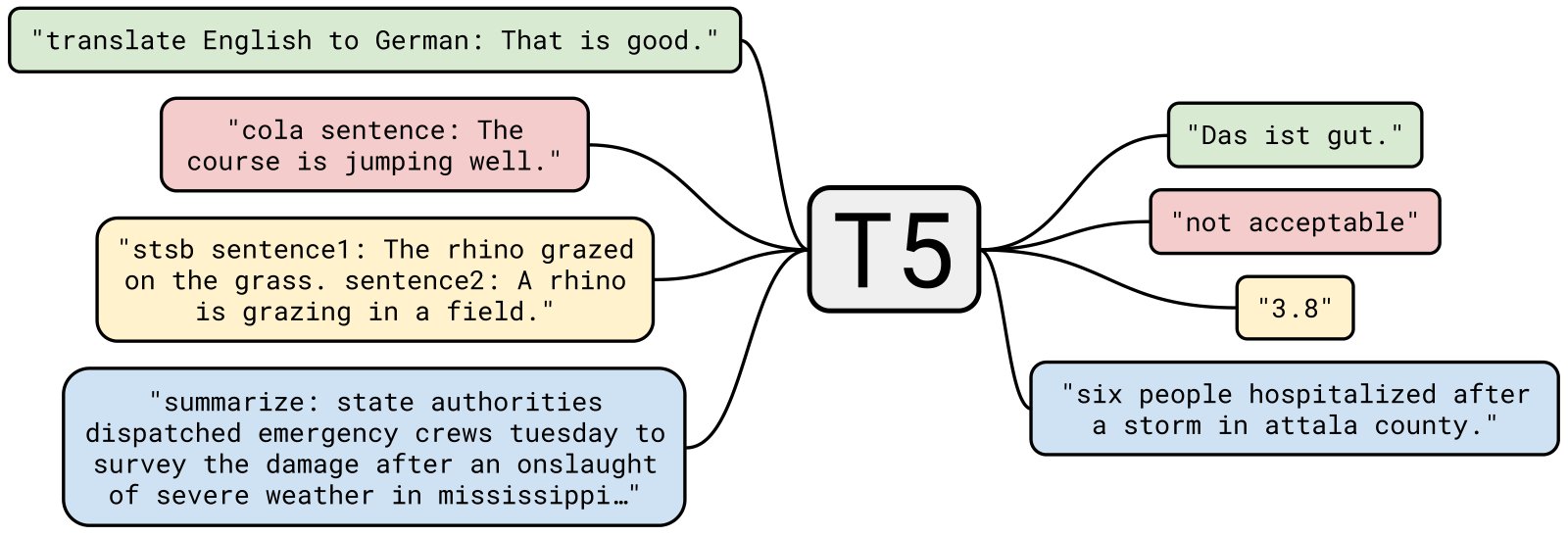
Figure 1: A diagram of our text-to-text framework. Every task we consider—including translation, question answering, and classification—is cast as feeding our model text as input and training it to generate some target text. This allows us to use the same model, loss function, hyperparameters, etc. across our diverse set of tasks. It also provides a standard testbed for the methods included in our empirical survey. “T5” refers to our model, which we dub the “Text-to-Text Transfer Transformer”.
图1:我们文本对文本框架图。 我们所考虑的每一项任务——包括翻译、问答和分类——都是为了提供我们的示范文本,作为投入和培训,以产生一些目标文本。 这使得我们能使用同样的模型,损失功能,超参数等,跨越我们不同的一组任务. 它还为我们的经验性调查所包含的方法提供了一个标准测试床。 “T5”是指我们的型号,我们把它称为证实了“Text-to-TextTransferTransformer”。
The basic idea underlying our work is to treat every text processing problem as a “text-to-text” problem, i.e. taking text as input and producing new text as output. This approach is inspired by previous unifying frameworks for NLP tasks, including casting all text problems as question answering (McCann et al. 2018), language modeling (Radford et al. 2019), or span extraction Keskar et al. 2019b tasks. Crucially, the text-to-text framework allows us to directly apply the same model, objective, training procedure, and decoding process to every task we consider. We leverage this flexibility by evaluating performance on a wide variety of English-based NLP problems, including question answering, document summarization, and sentiment classification, to name a few. With this unified approach, we can compare the effectiveness of different transfer learning objectives, unlabeled data sets, and other factors, while exploring the limits of transfer learning for NLP by scaling up models and data sets beyond what has previously been considered.
我们工作的基本思想是将每个文本处理问题视为一个“文本对文本”问题,即把文本当作投入和产生新的文本作为产出。 这种方法的灵感来自以往NLP任务的统一框架,包括将所有文本问题铸成问答(McCann等人,2018年),语言建模(Radford等人,2019年),或横跨提取Keskar等人,2019年b任务. 关键是,文本对文本的框架使我们能够直接将同样的模式、客观、培训程序和编解码程序应用于我们考虑的每一项任务。 我们利用这种灵活性,评估各种基于英语的NLP问题的业绩,包括回答问题、文件摘要和情绪分类等等。 通过这种统一的方法,我们可以比较不同的转移学习目标,无标签数据集和其他因素的有效性,同时通过扩大模型和数据集的范围,超越之前考虑的范围,探索NLP的转移学习的局限性.
We emphasize that our goal is not to propose new methods but instead to provide a comprehensive perspective on where the field stands. As such, our work primarily comprises a survey, exploration, and empirical comparison of existing techniques. We also explore the limits of current approaches by scaling up the insights from our systematic study (training models up to billion parameters) to obtain state-of-the-art results in many of the tasks we consider. In order to perform experiments at this scale, we introduce the “Colossal Clean Crawled Corpus” (C4), a data set consisting of hundreds of gigabytes of clean English text scraped from the web. Recognizing that the main utility of transfer learning is the possibility of leveraging pre-trained models in data-scarce settings, we release our code, data sets, and pre-trained models.1
我们强调,我们的目标不是提出新的方法,而是就实地状况提供全面的看法。 因此,我们的工作主要包括对现有技术的调查、探索和经验比较。 我们还通过扩大我们系统研究(培训模式高达XXMATH0.20亿参数)的洞察力,探索目前做法的局限性,以便在我们考虑的许多任务中获得最新成果。 为了进行这种规模的实验,我们引入了“Colossal Clean Crawled Corpus”(C4),这是一个由数百千兆字节从网络上刮掉的干净英文文本组成的数据集。 认识到转移学习的主要用途是在数据稀缺的设置中利用预先训练过的模型的可能性,我们释放了我们的代码,数据集和预先训练过的模型. 页:1
The remainder of the paper is structured as follows: In the following section, we discuss our base model and its implementation, our procedure for formulating every text processing problem as a text-to-text task, and the suite of tasks we consider. In Section 3, we present a large set of experiments that explore the field of transfer learning for NLP. At the end of the section (Section 3.7), we combine insights from our systematic study to obtain state-of-the-art results on a wide variety of benchmarks. Finally, we provide a summary of our results and wrap up with a look towards the future in Section 4.
本文件其余部分的结构如下: 在下一节中,我们讨论我们的基本模式及其执行情况,我们作为文本对文本任务拟定每个文本处理问题的程序,以及我们所考虑的一系列任务。 在第三节中,我们提出了一套大型的实验,探索NLP的转移学习领域. 在本节(第3.7节)末尾,我们综合了我们系统研究的见解,以便在各种基准方面取得最新成果。 最后,我们总结了我们的成果,最后在第4节中展望未来。
2 Setup
2 设置
Before presenting the results from our large-scale empirical study, we review the necessary background topics required to understand our results, including the Transformer model architecture and the downstream tasks we evaluate on. We also introduce our approach for treating every problem as a text-to-text task and describe our “Colossal Clean Crawled Corpus” (C4), the Common Crawl-based data set we created as a source of unlabeled text data. We refer to our model and framework as the “Text-to-Text Transfer Transformer” (T5).
在介绍我们大规模经验研究的结果之前,我们审查了解我们的结果所需的必要背景议题,包括Transformer模型架构和我们评价的下游任务。 我们还介绍了我们把每个问题作为文本对文本的任务处理的方法,并描述了我们作为未加标签的文本数据来源而创建的“Clossal Clean Crawled Corpus”(C4),即以Crawl为基础的共同数据集。 我们把我们的模型和框架称为“Text-to-TextTransfer” (T5)。
2.1 Model
2.1 模型
Early results on transfer learning for NLP leveraged recurrent neural networks (Peters et al. 2018; Howard and Ruder 2018), but it has recently become more common to use models based on the “Transformer” architecture (Vaswani et al. 2017). The Transformer was initially shown to be effective for machine translation, but it has subsequently been used in a wide variety of NLP settings (Radford et al. 2018; Devlin et al. 2018; McCann et al. 2018; Yu et al. 2018). Due to its increasing ubiquity, all of the models we study are based on the Transformer architecture. Apart from the details mentioned below and the variants we explore in Section 3.2, we do not deviate significantly from this architecture as originally proposed. Instead of providing a comprehensive definition of this model, we refer the interested reader to the original paper (Vaswani et al. 2017) or follow-up tutorials[^3],[^4] for a more detailed introduction.
NLP早期的转移学习结果利用了经常性神经网络(Peters等人,2018年;Howard和Ruder 2018年),但最近更常用的是使用基于"Transformer"架构的模型(Vaswani等人,2017年). "Transformer"最初被证明对机器翻译有效,但后来被用于多种NLP设置(拉德福德等人,2018年;德夫林等人,2018年;麦坎等人,2018年;尤等人,2018年). 由于它越来越普遍,我们研究的所有模型都基于Transformer架构. 除了下文提到的细节和我们在第3.2节中探讨的各种变体外,我们没有按照原先的建议,大大偏离这一结构。 我们没有为这一模式提供一个全面的定义,而是请感兴趣的读者参考原论文(Vaswani等人,2017年)或后续教程[^3],[^4],作为更详细的介绍.
The primary building block of the Transformer is self-attention (Cheng et al. 2016). Self-attention is a variant of attention (Graves 2013; Bahdanau et al. 2015) that processes a sequence by replacing each element by a weighted average of the rest of the sequence. The original Transformer consisted of an encoder-decoder architecture and was intended for sequence-to-sequence (Sutskever et al. 2014; Kalchbrenner et al. 2014) tasks. It has recently also become common to use models consisting of a single Transformer layer stack, with varying forms of self-attention used to produce architectures appropriate for language modeling (Radford et al. 2018; Al-Rfou et al. 2019) or classification and span prediction tasks (Devlin et al. 2018; Yang et al. 2019). We empirically explore these architectural variants in Section 3.2.
"变 你为什么要这样做"的主要构件是自觉的(Cheng等人,2016年)。 自觉是注意的一个变体(Graves 2013;Bahdanau等人,2015年),它通过将每个元素替换为其余序列的加权平均值来处理一个序列. 原Transformer由编码器-解码器架构组成,用于序列对序(Sutskever等人,2014年;Kalchbrenner等人,2014年)任务. 最近也常采用由单个Transformer层堆栈组成的模型,使用不同形式的自注意力来制作适合语言模型的架构(拉德福德等人,2018年;Al-Rfou等人,2019年)或分类和跨度预测任务(Devlin等人,2018年;杨等人,2019年). 我们在3.2节中以实证方式探索这些建筑变体.
Overall, our encoder-decoder Transformer implementation closely follows its originally-proposed form (Vaswani et al. 2017). First, an input sequence of tokens is mapped to a sequence of embeddings, which is then passed into the encoder. The encoder consists of a stack of “blocks”, each of which comprises two subcomponents: a self-attention layer followed by a small feed-forward network. Layer normalization (Ba et al. 2016) is applied to the input of each subcomponent. We use a simplified version of layer normalization where the activations are only rescaled and no additive bias is applied. After layer normalization, a residual skip connection (He et al. 2016) adds each subcomponent’s input to its output. Dropout (Srivastava et al. 2014) is applied within the feed-forward network, on the skip connection, on the attention weights, and at the input and output of the entire stack. The decoder is similar in structure to the encoder except that it includes a standard attention mechanism after each self-attention layer that attends to the output of the encoder. The self-attention mechanism in the decoder also uses a form of autoregressive or causal self-attention, which only allows the model to attend to past outputs. The output of the final decoder block is fed into a dense layer with a softmax output, whose weights are shared with the input embedding matrix. All attention mechanisms in the Transformer are split up into independent “heads” whose outputs are concatenated before being further processed.
总的来说,我们的编码器-解码器Transformer的采用与最初提议的形式(Vaswani等人,2017年)密切相仿。 首先,将一个输入序列的符号映射到一个嵌入序列,然后传入编码器. 编码器由一叠“块”组成,每个块由两个子部分组成:自留层,然后是小的向导网。 层态化(Ba等人,2016年)适用于每个子组件的输入. 我们使用简化版的层层正常化,其中的激活只进行重新标定,没有应用添加剂偏差. 在层态化后,一个剩余跳转连接(He等人,2016年)将每个子组件的输入加入到其输出中. 退学(Srivastava等人,2014年)在向导网络内应用,在跳过连接上应用,在注意力重量上应用,在整个堆栈的输入和输出上应用. 解码器在结构上与编码器相似,只是它包括一个标准注意机制,在每一个自注意力层后,都关注编码器的输出. 解码器中的自注意力机制也使用一种自注意力或因果自注意力的形式,只允许模型关注过去的输出. 最终解码器块的输出被装入一个具有软max输出的密集层,其重量与输入嵌入矩阵共享. " Transformer " 中的所有注意机制都分成独立的 " 头 " ,其产出在进一步处理之前就被压缩。
Since self-attention is order-independent (i.e. it is an operation on sets), it is common to provide an explicit position signal to the Transformer. While the original Transformer used a sinusoidal position signal or learned position embeddings, it has recently become more common to use relative position embeddings (Shaw et al. 2018; Huang et al. 2018a). Instead of using a fixed embedding for each position, relative position embeddings produce a different learned embedding according to the offset between the “key” and “query” being compared in the self-attention mechanism. We use a simplified form of position embeddings where each “embedding” is simply a scalar that is added to the corresponding logit used for computing the attention weights. For efficiency, we also share the position embedding parameters across all layers in our model, though within a given layer each attention head uses a different learned position embedding. Typically, a fixed number of embeddings are learned, each corresponding to a range of possible key-query offsets. In this work, we use embeddings for all of our models with ranges that increase in size logarithmically up to an offset of beyond which we assign all relative positions to the same embedding. Note that a given layer is insensitive to relative position beyond tokens, but subsequent layers can build a sensitivity to larger offsets by combining local information from previous layers. To summarize, our model is roughly equivalent to the original Transformer proposed by Vaswani et al. 2017 with the exception of removing the Layer Norm bias, placing the layer normalization outside the residual path, and using a different position embedding scheme. Since these architectural changes are orthogonal to the experimental factors we consider in our empirical survey of transfer learning, we leave the ablation of their impact for future work.
由于自我意向是命令独立的(即它是在sets上的操作),因此通常向Transformer提供明确的位置信号. 虽然最初的Transformer使用了鼻音位置信号或学习到的位置嵌入,但最近更常用的是相对位置嵌入(Shaw等人,2018年;Huang等人,2018年a). 相对位置嵌入法不是为每个位置使用固定嵌入法,而是根据自留置机制中比较的“钥匙”和“钥匙”之间的抵消,产生不同的已学习到的嵌入法。 我们使用一种简化的嵌入式位置形式,其中每个“嵌入”只是用于计算注意力权重的相应记录中添加的标尺。 为了提高效率,我们还分享我们模型中所有层的嵌入参数的位置,尽管在一个特定的层内,每个注意力头都使用不同的学习到的位置嵌入. 通常情况下,会学会固定的嵌入数,每个嵌入数对应一系列可能的密钥-query抵消. 在这项工作中,我们对所有模型使用嵌入法,其范围在大小对数上增加,最多可抵消,除此之外,我们将所有相对位置分配给同一嵌入法。 注意,一个给定的层对令牌以外的相对位置不敏感,但后续的层可以通过结合以前层的局部信息来建立对较大抵消的敏感性. 概括而言,我们的模型大致相当于瓦斯瓦尼等人2017年提出的原Transformer,除了去除层诺姆偏差,将层正常化置于剩余路径之外,以及使用不同位置嵌入方案. 由于这些建筑变化与我们在对转移学习的实证调查中考虑的实验因素是正统的,所以我们把其影响的减退留给今后的工作.
As part of our study, we experiment with the scalability of these models, i.e. how their performance changes as they are made to have more parameters or layers. Training large models can be non-trivial since they might not fit on a single machine and require a great deal of computation. As a result, we use a combination of model and data parallelism and train models on ‘‘slices’’ of Cloud TPU Pods.[^5] TPU pods are are multi-rack ML supercomputers that contain TPU v3 chips connected via a high-speed 2D mesh interconnect with supporting CPU host machines. We leverage the Mesh TensorFlow library (Shazeer et al. 2018) for ease of implementation of both model parallelism and data parallelism (Krizhevsky 2014).
作为我们研究的一部分,我们试验这些模型的可伸缩性,即它们的性能如何随着它们被制成更多的参数或层而改变. 训练大型模型可能是非三角型的,因为它们可能不适合单机,需要大量的计算. 因此,我们在Cloud TPU Pods的 QQslices 上采用了模型和数据并行论以及列车模型的组合. [^5] TPU pods是多轨ML超级计算机,包含 TPU v3芯片,通过高速2D网格连接与支持的CPU主机连接. 我们利用Mesh TensorFlow图书馆(Shazeer等人,2018年)方便实施模式并行主义和数据并行主义(Krizhevsky,2014年)。
2.2 The Colossal Clean Crawled Corpus
2.2 超大规模清洁爬取语料(C4)
Much of the previous work on transfer learning for NLP makes use of large unlabeled data sets for unsupervised learning. In this paper, we are interested in measuring the effect of the quality, characteristics, and size of this unlabeled data. To generate data sets that satisfy our needs, we leverage Common Crawl as a source of text scraped from the web. Common Crawl has previously been used as a source of text data for NLP, for example to train an n-gram language model (Buck et al. 2014), as training data for commonsense reasoning (Trinh and Le 2018), for mining parallel texts for machine translation (Smith et al. 2013), as a pre-training data set (Grave et al. 2018; Zellers et al. 2019; Liu et al. 2019c), and even simply as a giant text corpus for testing optimizers (Anil et al. 2019).
先前为NLP进行的转移学习工作,大多使用大型无标签数据集进行无监督学习. 在本文中,我们有兴趣测量这一无标签数据的质量、特点和大小的影响。 为了生成能满足我们需要的数据集,我们利用Common Crawl作为从网络中刮去的文本的来源. 常见的Crawl此前被用作NLP的文本数据源,例如用于培训n-gram语言模型(Buck等人,2014年),作为常识推理的培训数据(Trinh and Le 2018),用于为机器翻译挖掘平行文本(Smith等人,2013年),作为培训前数据集(Grave等人,2018年;Zellers等人,2019年;Liu等人,2019年c),甚至只是作为测试优化器的巨型文本体(Anil等人,2019年).
Common Crawl is a publicly-available web archive that provides “web extracted text” by removing markup and other non-text content from the scraped HTML files. This process produces around 20TB of scraped text data each month. Unfortunately, the majority of the resulting text is not natural language. Instead, it largely comprises gibberish or boiler-plate text like menus, error messages, or duplicate text. Furthermore, a good deal of the scraped text contains content that is unlikely to be helpful for any of the tasks we consider (offensive language, placeholder text, source code, etc.). To address these issues, we used the following heuristics for cleaning up Common Crawl’s web extracted text:
Crawl是一个可公开查阅的网页档案,它通过从已删除的 HTML 文件中删除标记和其他非文本内容来提供“web提取的文本”。 这个过程每月产生大约20TB的废文本数据. 遗憾的是,由此产生的案文大多数不是自然语言。 相反,它主要包括诸如菜单、错误信息或重复文本等粗略或锅炉板文本。 此外 当我们考虑任何任务时(攻击性语言、占位符文本、源代码等), 为了解决这些问题,我们用以下热度来清理共同爬行网摘录的文本:
- • We only retained lines that ended in a terminal punctuation mark (i.e. a period, exclamation mark, question mark, or end quotation mark).
- • We discarded any page with fewer than 3 sentences and only retained lines that contained at least 5 words.
- • We removed any page that contained any word on the ‘‘List of Dirty, Naughty, Obscene or Otherwise Bad Words’’.[^6]
- • Many of the scraped pages contained warnings stating that Javascript should be enabled so we removed any line with the word Javascript.
- • Some pages had placeholder “lorem ipsum” text; we removed any page where the phrase “lorem ipsum” appeared.
- • Some pages inadvertently contained code. Since the curly bracket “{” appears in many programming languages (such as Javascript, widely used on the web) but not in natural text, we removed any pages that contained a curly bracket.
- • Since some of the scraped pages were sourced from Wikipedia and had citation markers (e.g. [1], [citation needed], etc.), we removed any such markers.
- • Many pages had boilerplate policy notices, so we removed any lines containing the strings “terms of use”, “privacy policy”, “cookie policy”, “uses cookies”, “use of cookies”, or “use cookies”.
- • To deduplicate the data set, we discarded all but one of any three-sentence span occurring more than once in the data set.
- 我们只保留以终点标注结束的线路(即一段期、感叹号、问号或最后引号)。
- 我们删除了任何小于3句的页面,只保留至少5个字的行。
- 我们删除了任何含有“肮脏、猥亵、淫秽或其他坏话清单”任何词的页面。
- 许多被刮掉的页中含有警告,说明应该启用Javascript,所以我们删除了任何与Javascript一词的行.
- 有些页有“自然”的占位词;我们删除了出现“自然”一词的任何页。
- 一些网页无意中载有代码。 由于卷轴括号“{”出现在许多编程语言中(如在网络上广泛使用的Javascript),但不出现在自然文本中,因此我们删除了含有卷轴括号的任何页面。
- 由于一些被刮掉的页面来自维基百科,并有引用标记(如[1],[需要引用]等),我们删除了任何此类标记.
- 许多页都有锅炉板政策通知,因此,我们删除了包含“使用条件”、“隐私政策”、“饼干政策”、“使用饼干”、“使用饼干”或“使用饼干”的任何线条。
- 为了简化数据集,我们放弃了数据集中不止一次发生的除一个之外的所有三刑期。
Additionally, since most of our downstream tasks are focused on English-language text, we used langdetect[^7] to filter out any pages that were not classified as English with a probability of at least 0.99. Our heuristics are inspired by past work on using Common Crawl as a source of data for NLP: For example, Grave et al. 2018 also filter text using an automatic language detector and discard short lines and Smith et al. 2013; Grave et al. 2018 both perform line-level deduplication. However, we opted to create a new data set because prior data sets use a more limited set of filtering heuristics, are not publicly available, and/or are different in scope (e.g. are limited to News data (Zellers et al. 2019; Liu et al. 2019c), comprise only Creative Commons content (Habernal et al. 2016), or are focused on parallel training data for machine translation (Smith et al. 2013)).
此外,由于我们下游的任务大多集中在英语文本上,我们使用langdetect[^7]来过滤任何未归类为英语的页面,其概率至少为0.99. 我们的heuristic受到过去使用Common Crawl作为NLP数据来源的工作的启发: 例如,Grave等人2018也使用自动语言探测器过滤文本,并丢弃短线;Smith等人2013年;Grave等人2018都进行线级疏解. 然而,我们选择建立一套新的数据集,因为以前的数据集使用比较有限的一套过滤heuristics,不公开,和/或范围不同(例如仅限于News数据(Zellers等人,2019年;Liu等人,2019年c),只包含Creative Commons内容(Habernal等人,2016年),或侧重于机器翻译的平行培训数据(Smith等人,2013年))。
To assemble our base data set, we downloaded the web extracted text from April 2019 and applied the aforementioned filtering. This produces a collection of text that is not only orders of magnitude larger than most data sets used for pre-training (about 750 GB) but also comprises reasonably clean and natural English text. We dub this data set the “Colossal Clean Crawled Corpus’’ (or C4 for short) and release it as part of TensorFlow Datasets.[^8] We consider the impact of using various alternative versions of this data set in Section 3.4.
为了组装我们的基础数据集,我们下载了2019年4月的网络提取文本,并应用了上述过滤. 由此收集的文本不仅比大多数用于预训的数据集(约750 GB)的数量级要大,而且包含相当干净和自然的英文文本. 我们将这一数据集编为“COlossalCLear”CLearedCorpus’’(或简称C4),并作为TensorFlow数据集的一部分发布。 我们考虑使用第3.4节中这一数据集的各种替代版本的影响。
2.3 Downstream Tasks
2.3 下游任务
Our goal in this paper is to measure general language learning abilities. As such, we study downstream performance on a diverse set of benchmarks, including machine translation, question answering, abstractive summarization, and text classification. Specifically, we measure performance on the GLUE and SuperGLUE text classification meta-benchmarks; CNN/Daily Mail abstractive summarization; SQuAD question answering; and WMT English to German, French, and Romanian translation. All data was sourced from TensorFlow Datasets.[^9]
我们在本文中的目标是衡量一般语言学习能力. 因此,我们研究了下游的一套不同基准的业绩,包括机器翻译、问答、抽象总结和文本分类。 具体来说,我们测量GLUE和SuperGLUE文本分类元基准;CNN/Daily Mail抽象总结;SQuAD问题回答;WMT英语到德语、法语和罗马尼亚语翻译。 所有数据都来自 TensorFlow 数据集。 [^9]
GLUE (Wang et al. 2018) and SuperGLUE (Wang et al. 2019b) each comprise a collection of text classification tasks meant to test general language understanding abilities:
GLUE(Wang等人,2018年)和SuperGLUE(Wang等人,2019年b)各包含一批文字分类任务,旨在测试一般语言理解能力: 语言理解能力:
- • Sentence acceptability judgment (CoLA (Warstadt et al. 2018))
- • Sentiment analysis (SST-2 (Socher et al. 2013))
- • Paraphrasing/sentence similarity (MRPC (Dolan and Brockett 2005), STS-B (Cer et al. 2017), QQP (Iyer et al. 2017))
- • Natural language inference (MNLI (Williams et al. 2017), QNLI (Rajpurkar et al. 2016), RTE (Dagan et al. 2005), CB (De Marneff et al. 2019))
- • Coreference resolution (WNLI and WSC (Levesque et al. 2012))
- • Sentence completion (COPA (Roemmele et al. 2011))
- • Word sense disambiguation (WIC (Pilehvar and Camacho-Collados 2018))
- • Question answering (MultiRC (Khashabi et al. 2018), ReCoRD (Zhang et al. 2018), BoolQ (Clark et al. 2019))
- 判刑可接受性判决(CoLA(Warstadt等人,2018年))
• 感官分析(SST-2(Socher等人,2013年))
• 审案/判决相似性(MRPC(Dolan和Brockett,2005年)、STS-B(Cer等人,2017年)、QQP(Iyer等人,2017年)) - 自然语言推论(MNLI(Williams等人,2017年)、QNLI(Rajpurkar等人,2016年)、RTE(Dagan等人,2005年)、CB(De Marneff等人,2019年))
• 参照决议(WNLI和WSC(Levesque等人,2012年))
• 判决完成情况(COPA(Roemmele等人,2011年))
· 语言感知分裂(WIC(Pilehvar和Camacho-Collados 2018)) - 回答问题(多资源中心(Khashabi等人,2018年)、ReCORD(Zhang等人,2018年)、BoolQ(Clark等人,2019年))
We use the data sets as distributed by the GLUE and SuperGLUE benchmarks. For simplicity, when fine-tuning we treat all of the tasks in the GLUE benchmark (and similarly for SuperGLUE) as a single task by concatenating all of the constituent data sets. As suggested by Kocijan et al. 2019 we also include the Definite Pronoun Resolution (DPR) data set (Rahman and Ng 2012) in the combined SuperGLUE task.
我们使用由GLUE和SuperGLUE基准分配的数据集. 简而言之,微调时,我们将GLUE基准中的所有任务(对于SuperGLUE来说也是类似的)作为一个单一任务,通过调整所有组成数据集. 正如Kocijan等人2019年建议的那样,我们还把Definite Pronoun分辨率(DPR)数据集(Rahman和Ng 2012)纳入合并的SuperGLUE任务中.
The CNN/Daily Mail (Hermann et al. 2015) data set was introduced as a question-answering task but was adapted for text summarization by Nallapati et al. 2016; we use the non-anonymized version from See et al. 2017 as an abstractive summarization task. SQuAD (Rajpurkar et al. 2016) is a common question-answering benchmark. In our experiments, the model is fed the question and its context and asked to generate the answer token-by-token. For WMT English to German, we use the same training data as (Vaswani et al. 2017) (i.e. News Commentary v13, Common Crawl, Europarl v7) and newstest2013 as a validation set (Bojar et al. 2014). For English to French, we use the standard training data from 2015 and newstest2014 as a validation set (Bojar et al. 2015). For English to Romanian, which is a standard lower-resource machine translation benchmark, we use the train and validation sets from WMT 2016 (Bojar et al. 2016). Note that we only pre-train on English data, so in order to learn to translate a given model will need to learn to generate text in a new language.
CNN/Daily Mail(Hermann et al. 2015)数据集作为问答任务推出,但由Nallapati et al. 2016进行文字总结修改;我们使用来自See et al. 2017的非匿名版本作为抽象总结任务. SQuAD(Rajpurkar等人,2016年)是一个常见的问答基准. 在我们的实验中,模型被输入了问题及其背景,并被要求逐个生成答案符号. 对于WMT英语到德语,我们使用与(Vaswani等人,2017年)相同的训练数据(即新闻评论v13,Common Crawl,Europal v7)和新闻test2013作为验证集(Bojar等人,2014年). 对于英语到法语,我们使用2015年的标准培训数据以及Newstest2014作为验证集(Bojar等人,2015年). 对于英语到罗马尼亚语,这是一个标准的低资源机器翻译基准,我们使用来自WMT 2016(Bojar等人,2016年)的列车和验证集. 请注意,我们只进行英语数据的预训,所以为了学习翻译一个特定的模型,需要学习用新语言生成文本.
2.4 Input and Output Format
2.4 输入与输出格式
In order to train a single model on the diverse set of tasks described above, we cast all of the tasks we consider into a “text-to-text” format—that is, a task where the model is fed some text for context or conditioning and is then asked to produce some output text. This framework provides a consistent training objective both for pre-training and fine-tuning. Specifically, the model is trained with a maximum likelihood objective (using “teacher forcing” (Williams and Zipser 1989)) regardless of the task. To specify which task the model should perform, we add a task-specific (text) prefix to the original input sequence before feeding it to the model.
为了就上述各种任务培训一个单一的模型,我们将我们所考虑的所有任务投入到一种 " 文字对文字 " 的格式中,即一种任务,即向模型提供一些文字供上下文或条件,然后要求它产生一些产出文本。 这一框架为培训前和调整提供了一致的培训目标。 具体来说,无论任务如何,该模式都以最大可能性目标(使用“教师强迫”(Williams和Zipser,1989年))加以培训。 要指定模型应该执行哪项任务,我们先在原始输入序列中添加一个任务特定(文本)前缀,然后再将其输入模型.
As an example, to ask the model to translate the sentence “That is good.” from English to German, the model would be fed the sequence “translate English to German: That is good.” and would be trained to output “Das ist gut.” For text classification tasks, the model simply predicts a single word corresponding to the target label. For example, on the MNLI benchmark (Williams et al. 2017) the goal is to predict whether a premise implies (“entailment”), contradicts (“contradiction”), or neither (“neutral”) a hypothesis. With our preprocessing, the input sequence becomes “mnli premise: I hate pigeons. hypothesis: My feelings towards pigeons are filled with animosity.” with the corresponding target word “entailment”. Note that an issue arises if our model outputs text on a text classification task that does not correspond to any of the possible labels (for example if the model outputs “hamburger” when the only possible labels for a task were “entailment”, “neutral”, or “contradiction”). In this case, we always count the model’s output as wrong, though we never observed this behavior in any of our trained models. Note that the choice of text prefix used for a given task is essentially a hyperparameter; we found that changing the exact wording of the prefix had limited impact and so did not perform extensive experiments into different prefix choices. A diagram of our text-to-text framework with a few input/output examples is shown in Figure 1. We provide full examples of preprocessed inputs for every task we studied in Appendix D.
例如,请模型将“这是好的 ” 句子从英文翻译成德文,该模型将输入“把英文翻译成德文:这是好的 ” 的序列,并将接受培训以输出“Das ist gut ” 。 对于文本分类任务,模型只是预测一个对应目标标签的单词. 例如,在MNLI基准(Williams 等人,2017年)上,目标是预测一个前提是否意味着“尾声”),是否与一个假设相矛盾,或者两个假设都不相矛盾。 随着我们的预处理,输入序列成为“mnli前提:我讨厌鸽子。 假设:我对鸽子的感情充满敌意。” 请注意,如果我们的关于文本分类任务的示范产出文本与任何可能的标签不符,就会产生一个问题(例如,当一项任务的唯一可能标签是“贴近”、“中性”或“约束”时,示范产出“汉堡”)。 在这种情况下,我们总是将模型的输出算作错误,尽管我们从未在任何经过训练的模型中观察到过这种行为. 注意特定任务使用的文本前缀的选择本质上是一个超参数;我们发现修改前缀的准确措辞影响有限,因此没有进行广泛的实验,改为不同的前缀选择. 图1显示了我们文本对文本框架的图表,其中有一些投入/产出实例。 我们为附录D中研究的每一项任务提供了经过预先处理的投入的全部例子。
Our text-to-text framework follows previous work that casts multiple NLP tasks into a common format: McCann et al. 2018 propose the “Natural Language Decathlon”, a benchmark that uses a consistent question-answering format for a suite of ten NLP tasks. The Natural Language Decathlon also stipulates that all models must be multi-task, i.e. are able to simultaneously tackle all of the tasks at once. We instead allow for separately fine-tuning the model on each individual task and use short task prefixes instead of an explicit question-answer format. Radford et al. 2019 evaluate the zero-shot learning capabilities of language models by feeding some input to the model as a prefix and then autoregressively sampling an output. For example, automatic summarization is done by feeding in a document followed by the text “TL;DR:” (short for “too long, didn’t read”, a common abbreviation) and then the summary is predicted via autoregressive decoding. We mainly consider models that explicitly process an input with an encoder before generating an output with a separate decoder and we focus on transfer learning rather than zero-shot learning. Finally, Keskar et al. 2019b unify many NLP tasks as “span extraction”, where text corresponding to possible output choices are appended to the input and the model is trained to extract the input span corresponding to the correct choice. In contrast, our framework also allows for generative tasks like machine translation and abstractive summarization where it is not possible to enumerate all possible output choices.
我们的文本对文本框架沿用了之前将多个NLP任务置于一个共同格式的工作:McCann 等人 2018年提出"自然语言Decathlon",这个基准为一套NLP任务使用一致的问答格式. "自然语言"(Natural Language Decathlon)也规定,所有模型都必须是多任务,即能够同时处理所有任务. 相反,我们允许对每个单独任务的模型分别进行微调,并使用简短的任务前缀而不是明确的问答格式。 Radford等人2019评价了语言模型的零弹射学习能力,将一些投入作为前缀提供给模型,然后自动对一个输出进行采样. 例如,自动归纳是通过在“TL;DR:”之后的文档中输入(简写为“太长,没有读过”,一个常用缩写),然后通过自动递归解码来预测汇总。 我们主要考虑的是,在用单独的解码器生成一个输出之前,用编码器明确处理输入的模型,我们侧重于转移学习而不是零镜头学习. 最后,Keskar 等人 2019b 将许多 NLP 任务统一为 “ span 提取 ” , 其中与可能输出选择对应的文本附在输入后,并且该模型经过培训以提取与正确选择相对应的输入跨度。 相比之下,我们的框架也允许诸如机器翻译和抽象归纳等遗传性任务,因为不可能列举所有可能的输出选择。
We were able to straightforwardly cast all of the tasks we considered into a text-to-text format with the exception of STS-B, which is a regression task where the goal is to predict a similarity score between and . We found that most of these scores were annotated in increments of , so we simply rounded any score to the nearest increment of and converted the result to a literal string representation of the number (e.g. the floating-point value would be mapped to the string “2.6”). At test time, if the model outputs a string corresponding to a number between and , we convert it to a floating-point value; otherwise, we treat the model’s prediction as incorrect. This effectively recasts the STS-B regression problem as a 21-class classification problem.
我们能够直接将我们所审议的所有任务都转化为文本对文本格式,但STS-B除外,这是一个回归式任务,目标是预测和之间的相似性分数。 我们发现,这些分数大多以的增量注出,因此我们简单地将任何分数四舍五入到最近的增量,并将结果转换为数字的字串表示(例如,浮动点值将映射到字符串“2.26”). 在测试时,如果模型输出一个与和之间的数字相对应的字符串,我们把它转换成浮点值;否则,我们将模型的预测视为不正确. 这有效地将STS-B回归问题改写为21级分类问题.
Separately, we also convert the Winograd tasks (WNLI from GLUE, WSC from SuperGLUE, and the DPR data set we add to SuperGLUE) into a simpler format that is more amenable to the text-to-text framework. Examples from the Winograd tasks consist of a text passage containing an ambiguous pronoun that could refer to more than one of the noun phrases in the passage. For example, the passage might be “The city councilmen refused the demonstrators a permit because they feared violence.”, which contains the ambiguous pronoun “they” that could refer to “city councilmen” or “demonstrators”. We cast the WNLI, WSC, and DPR tasks as text-to-text problems by highlighting the ambiguous pronoun in the text passage and asking the model to predict the noun that it refers to. The example mentioned above would be transformed to the input “The city councilmen refused the demonstrators a permit because they feared violence.” and the model would be trained to predict the target text “The city councilmen”.
另外,我们还将W作了答复的Winograd任务(WNLI从GLUE,WSC从SuperGLUE,以及我们添加到SuperGLUE的DPR数据集)转换为更适合文本对文本框架的更简单格式. 维诺格勒任务的例子包括一个文本段落中包含一个模糊的代词,可以指该段落中不止一个名词短语. 例如,这段话可能是“市议员因害怕暴力而拒绝示威者的许可”,其中含有含糊的“他们”一词,可以指“市议员”或“示威者”。 我们把WNLI,WSC和DPR任务作为文本对文本的问题,在文本段落中强调模棱两可的代词,并要求模型预测它所提到的名词. 上面提到的例子将变为“市议员拒绝给示威者发放许可证,因为他们* 害怕暴力。” 模型将接受培训,以预测目标文字“市议员”。
For WSC, examples contain the passage, the ambiguous pronoun, a candidate noun, and a True/False label reflecting whether the candidate matches the pronoun (ignoring any articles). We only train on examples with a “True” label since we do not know the correct noun targets for examples with a “False” label. For evaluation, we assign a “True” label if the words in the model’s output are a subset of the words in the candidate noun phrase (or vice versa) and assign a “False” label otherwise. This removes roughly half of the WSC training set, but the DPR data set adds about pronoun resolution examples. Examples from DPR are annotated with the correct referent noun, making it easy to use this data set in the format listed above.
对于WSC来说,例子包括段落,模棱两可的代词,候选名词,以及反映候选名词是否与代词匹配的True/False标签(在任何文章上发声). 我们只是用“真”标签来培训例子,因为我们不知道有“假”标签的例子的正确名词目标。 对于评价,如果模型输出中的单词是候选名词短语(反之亦然)中单词的子集,我们就会指定一个 " True " 标签,并另指定一个 " False " 标签。 这移除了大约一半的WSC训练集,但DPR数据集增加了大约代名词解析实例. DPR中的实例以正确的参考名词注解,使得使用上述格式的本数据集变得容易.
The WNLI training and validation sets have a significant overlap with the WSC training set. To avoid leaking validation examples into our training data (a particular issue in the multi-task experiments of Section 3.5.2), we therefore never train on WNLI and never report results on the WNLI validation set. Omitting results on the WNLI validation set is standard practice (Devlin et al. 2018) due to the fact that it is “adversarial” with respect to the training set, i.e. validation examples are all slightly-perturbed versions of training examples with the opposite label. As such, we do not include WNLI in the average GLUE score whenever we report on the validation set (all sections except Section 3.7 where results are presented on the test sets). Converting examples from WNLI to the “referent noun prediction” variant described above is a little more involved; we describe this process in Appendix B.
WNLI的培训和验证装置与WSC的训练装置有很大的重叠. 因此,为了避免将验证实例泄露到我们的培训数据中(第3.5.2节的多任务实验中的一个具体问题),我们从未对WNLI进行培训,也从未报告WNLI验证集的结果。 WNLI验证集的观测结果是标准做法(Devlin等人,2018年),因为它对训练集是"对抗性"的,即验证实例都是带有相反标签的训练实例的轻微扰动版本. 因此,我们每次报告验证组(除第3.7节在测试组上提交结果)时,都不将WNLI列入平均GLUE分数。 将例子从WNLI转换为上文所述的“参考名词预测”变体,参与程度略高;我们在附录B中描述了这一过程。
3 Experiments
3 实验
Recent advances in transfer learning for NLP have come from a wide variety of developments, such as new pre-training objectives, model architectures, unlabeled data sets, and more. In this section, we carry out an empirical survey of these techniques in hopes of teasing apart their contribution and significance. We then combine the insights gained to attain state-of-the-art in many of the tasks we consider. Since transfer learning for NLP is a rapidly growing area of research, it is not feasible for us to cover every possible technique or idea in our empirical study. For a broader literature review, we recommend a recent survey by Ruder et al. 2019.
近期NLP的转移学习进展来自多种发展,如新的培训前目标,模型架构,无标签数据集等等. 在本节中,我们对这些技术进行了实证调查,希望它们能够发挥各自的贡献和意义。 然后,我们综合了我们所考虑的许多任务中为达到最新水平而取得的见解。 由于NLP的转学学习是一个迅速增长的研究领域,因此我们无法在经验研究中涵盖每一种可能的技术或想法. 为了进行更广泛的文献审查,我们推荐鲁德等人最近的一项调查. 2019.
We systematically study these contributions by taking a reasonable baseline (described in Section 3.1) and altering one aspect of the setup at a time. For example, in Section 3.3 we measure the performance of different unsupervised objectives while keeping the rest of our experimental pipeline fixed. This “coordinate ascent” approach might miss second-order effects (for example, some particular unsupervised objective may work best on a model larger than our baseline setting), but performing a combinatorial exploration of all of the factors in our study would be prohibitively expensive. In future work, we expect it could be fruitful to more thoroughly consider combinations of the approaches we study.
我们系统地研究这些贡献,采用合理的基线(在第3.1节中说明),并一次改变设置的一个方面。 例如,在第3.3节中,我们衡量不同无监督目标的绩效,同时维持我们试验管道的其余部分。 这种“协调上升”的办法可能忽略了二阶效应(例如,一些特定不受监督的目标在超出我们基准设定的模型上可能最有效),但对我们的研究中的所有因素进行组合性探讨将极为昂贵。 在今后的工作中,我们期望更彻底地考虑我们所研究的各种办法的结合,是能够取得成果的。
Our goal is to compare a variety of different approaches on a diverse set of tasks while keeping as many factors fixed as possible. In order to satisfy this aim, in some cases we do not exactly replicate existing approaches. For example, “encoder-only” models like BERT (Devlin et al. 2018) are designed to produce a single prediction per input token or a single prediction for an entire input sequence. This makes them applicable for classification or span prediction tasks but not for generative tasks like translation or abstractive summarization. As such, none of the model architectures we consider are identical to BERT or consist of an encoder-only structure. Instead, we test approaches that are similar in spirit—for example, we consider an analogous objective to BERT’s “masked language modeling” objective in Section 3.3 and we consider a model architecture that behaves similarly to BERT on text classification tasks in Section 3.2.
我们的目标是在尽可能多地确定因素的同时,就一套不同的任务比较各种不同的办法。 为了实现这一目标,在某些情况下,我们并不完全照搬现有的办法。 例如,BERT(Devlin等人,2018年)等“仅编码器”模型旨在为整个输入序列产生每个输入符的单一预测或单一预测。 这使得它们适用于分类或跨度预测任务,但不适用于翻译或抽象归纳等遗传性任务. 因此,我们认为的模型架构中没有一个与BERT完全相同,或者由一个只编码器的结构组成. 相反,我们检验了精神上相似的方法——例如,我们认为,与BERT在第3.3节中的 " 假冒语言模型 " 目标类似的目标,我们认为,在3.2节的案文分类任务上,示范结构的表现与BERT相似。
After outlining our baseline experimental setup in the following subsection, we undertake an empirical comparison of model architectures (Section 3.2), unsupervised objectives (Section 3.3), pre-training data sets (Section 3.4), transfer approaches (Section 3.5), and scaling (Section 3.6). At the culmination of this section, we combine insights from our study with scale to obtain state-of-the-art results in many tasks we consider (Section 3.7).
在以下小节中概述了我们的基线实验设置之后,我们对模型结构(第3.2节)、不受监督的目标(第3.3节)、培训前数据集(第3.4节)、转移方法(第3.5节)和规模(第3.6节)进行了实证比较。 在本节的高潮中,我们将我们研究的见解与规模结合起来,以便在我们考虑的许多任务中取得最新成果(第3.7节)。
3.1 Baseline
3.1 基线
Our goal for our baseline is to reflect typical, modern practice. We pre-train a standard Transformer (described in Section 2.1) using a simple denoising objective and then separately fine-tune on each of our downstream tasks. We describe the details of this experimental setup in the following subsections.
我们的基线目标是反映典型的现代做法。 我们预先训练一个标准Transformer(在第2.1节中描述),使用一个简单的去名目标,然后对我们的每一项下游任务分别进行微调. 我们在以下各小节中描述了这一实验设置的细节.
3.1.1 Model
For our model, we use a standard encoder-decoder Transformer as proposed by Vaswani et al. 2017. While many modern approaches to transfer learning for NLP use a Transformer architecture consisting of only a single “stack” (e.g. for language modeling (Radford et al. 2018; Dong et al. 2019) or classification and span prediction (Devlin et al. 2018; Yang et al. 2019)), we found that using a standard encoder-decoder structure achieved good results on both generative and classification tasks. We explore the performance of different model architectures in Section 3.2.
3.1.1 型号
对于我们的模型,我们使用由Vaswani等人2017年提出的标准编码器-解码器Transformer. 虽然许多用于NLP的现代转学方法使用只有单个"链条"(如语言建模(Radford等人,2018年;Dong等人,2019年))或分类和跨度预测(Devlin等人,2018年;Yang等人,2019年)组成的Transformer架构,但我们发现,使用标准编码器-解码器结构在基因和分类任务上都取得了良好的成果. 我们探索3.2节不同模型建筑的性能.
Our baseline model is designed so that the encoder and decoder are each similar in size and configuration to a “BERTBASE” (Devlin et al. 2018) stack. Specifically, both the encoder and decoder consist of blocks (each block comprising self-attention, optional encoder-decoder attention, and a feed-forward network). The feed-forward networks in each block consist of a dense layer with an output dimensionality of followed by a ReLU nonlinearity and another dense layer. The “key” and “value” matrices of all attention mechanisms have an inner dimensionality of and all attention mechanisms have heads. All other sub-layers and embeddings have a dimensionality of . In total, this results in a model with about million parameters. This is roughly twice the number of parameters of BERTBASE since our baseline model contains two layer stacks instead of one. For regularization, we use a dropout probability of everywhere dropout is applied in the model.
我们的基准模型的设计使得编码器和解码器在大小和配置上都与一个“BERTBASE”(Devlin等人,2018年)堆栈类似。 具体来说,编码器和解码器都由区块(每个区块包括自注意力,可选的编码器解码器注意,以及一个向导网络)组成. 每个区块的向导网络由一个输出维度为的密集层组成,然后是ReLU非线性层和另一个密集层。 所有关注机制的“关键”和“价值”矩阵具有的内在维度,所有关注机制都有的头。 所有其他子层和嵌入层的维度为. 总的来说,这形成了一个拥有大约百万参数的模型. 这大约是BERTBASE参数的两倍,因为我们的基准模型包含两个层叠而不是一个。 在正规化方面,模式中采用了每处辍学概率。
3.1.2 Training
As described in Section 2.4, all tasks are formulated as text-to-text tasks. This allows us to always train using standard maximum likelihood, i.e. using teacher forcing (Williams and Zipser 1989) and a cross-entropy loss. For optimization, we use AdaFactor (Shazeer and Stern 2018). At test time, we use greedy decoding (i.e. choosing the highest-probability logit at every timestep).
3.1.2 培训
如第2.4节所述,所有任务都作为文本对文本的任务拟订。 这使得我们总是可以使用标准的最大可能性来进行训练,即使用教师强迫(Williams和Zipser 1989)和交叉性的损失. 为了优化,我们使用AdaFactor(Shazeer和Stern 2018). 在测试时,我们使用贪婪的解码(即在每个时步选择最高概率的登录).
We pre-train each model for steps on C4 before fine-tuning. We use a maximum sequence length of and a batch size of sequences. Whenever possible, we ‘‘pack’’ multiple sequences into each entry of the batch[^10] so that our batches contain roughly tokens. In total, this batch size and number of steps corresponds to pre-training on tokens. This is considerably less than BERT (Devlin et al. 2018), which used roughly tokens, or RoBERTa (Liu et al. 2019c), which used roughly tokens. Using only tokens results in a reasonable computational budget while still providing a sufficient amount of pre-training for acceptable performance. We consider the effect of pre-training for more steps in Sections 3.6 and 3.7. Note that tokens only covers a fraction of the entire C4 data set, so we never repeat any data during pre-training.
我们在微调前先对每款型号进行XMATH0XX步骤在C4上的预训. 我们使用最大序列长度为,批量大小为序列. 只要有可能,我们就会在批[^10]的每个条目中装入多个序列,使我们的批次包含大约令牌。 总的来说,这种批量大小和步数对应令牌的预训. 这大大低于BERT(Devlin等人,2018年),后者大约使用令牌,或RoBERTa(Liu等人,2019年c),后者大约使用令牌. 仅使用令牌就产生了合理的计算预算,同时仍然为可接受的业绩提供足够数量的预训. 我们认为预训对第3.6节和第3.7节中更多步骤的影响。 请注意,令牌只涵盖整个C4数据集的一小部分,因此我们在预训期间从未重复过任何数据.
During pre-training, we use an “inverse square root” learning rate schedule: where is the current training iteration and is the number of warm-up steps (set to in all of our experiments). This sets a constant learning rate of for the first steps, then exponentially decays the learning rate until pre-training is over. We also experimented with using a triangular learning rate (Howard and Ruder 2018), which produced slightly better results but requires knowing the total number of training steps ahead of time. Since we will be varying the number of training steps in some of our experiments, we opt for the more generic inverse square root schedule.
在预训期间,我们使用“反方根”学习率表:,其中是目前的训练迭代,是热身步骤的数量(我们所有实验中设定为)。 这为第一个步骤设定了的恒定学习速率,然后指数化地衰减学习速率直至预训结束. 我们还试用了三角学习率(Howard和Ruder 2018),取得了略好的结果,但需要提前了解培训步骤的总数。 由于我们将在有些实验中改变训练步骤的数量,我们选择比较通用的反方根表.
Our models are fine-tuned for steps on all tasks. This value was chosen as a trade-off between the high-resource tasks (i.e. those with large data sets), which benefit from additional fine-tuning, and low-resource tasks (smaller data sets), which overfit quickly. During fine-tuning, we continue using batches with length- sequences (i.e. tokens per batch). We use a constant learning rate of when fine-tuning. We save a checkpoint every steps and report results on the model checkpoint corresponding to the highest validation performance. For models fine-tuned on multiple tasks, we choose the best checkpoint for each task independently. For all of the experiments except those in Section 3.7, we report results in the validation set to avoid performing model selection on the test set.
我们的模型被精细调整,用于所有任务的步骤. 这一数值被选作高资源任务(即那些拥有大数据集的任务)与低资源任务(更小的数据集)之间的权衡,后者得益于额外的微调,而后者很快的过于匹配. 在微调期间,我们继续使用带有长度-序列的批次(即每批令牌). 我们在微调时使用的恒定学习率. 我们每个步骤都省下一个检查站,并报告模型检查站对应于最高验证性能的结果. 对于对多个任务进行微调的模型,我们独立选择每个任务的最佳检查点. 除了3.7节的实验外,我们报告验证组的结果,以避免在测试组上进行模型选择。
3.1.3 Vocabulary
We use SentencePiece (Kudo and Richardson 2018) to encode text as WordPiece tokens (Sennrich et al. 2015; Kudo 2018). For all experiments, we use a vocabulary of wordpieces. Since we ultimately fine-tune our model on English to German, French, and Romanian translation, we also require that our vocabulary covers these non-English languages. To address this, we classified pages from the Common Crawl scrape used in C4 as German, French, and Romanian. Then, we trained our SentencePiece model on a mixture of parts of English C4 data with part each of data classified as German, French or Romanian. This vocabulary was shared across both the input and output of our model. Note that our vocabulary makes it so that our model can only process a predetermined, fixed set of languages.
3.1.3 词汇
我们使用PriedPiece(Kudo and Richardson 2018)将文本编码为WordPiece符(Sennrich et al. 2015;Kudo 2018). 对所有实验,我们使用词组的词汇. 由于我们最终微调了英语到德语、法语和罗马尼亚语的翻译模式,我们也要求我们的词汇涵盖这些非英语语言。 为了解决这个问题,我们把C4中使用的Crawl scrape中的网页归类为德语、法语和罗马尼亚语。 然后,我们训练了我们的PrisonPi spiderce模型, 将英国C4数据的部分与部分混合在一起, 每个数据被归类为德国,法国或罗马尼亚. 我们的模型投入和产出都分享了这一词汇。 请注意,我们的词汇使得我们的模型只能处理一套预定的,固定的语言.
3.1.4 Unsupervised Objective
Figure 2: Schematic of the objective we use in our baseline model. In this example, we process the sentence “Thank you for inviting me to your party last week.” The words “for”, “inviting” and “last” (marked with an ) are randomly chosen for corruption. Each consecutive span of corrupted tokens is replaced by a sentinel token (shown as and ) that is unique over the example. Since “for” and “inviting” occur consecutively, they are replaced by a single sentinel . The output sequence then consists of the dropped-out spans, delimited by the sentinel tokens used to replace them in the input plus a final sentinel token .
3.1.4 无监督的目标
图2:我们在基线模型中使用的目标的示意图。 在这个例子中,我们处理“感谢你上周邀请我参加你的聚会”这句话。 随意选用“用于”、“邀请”和“最后”(标注为)等词作为腐败罪。 每个连续的损坏的代币都被一个哨音代币(shown as QQ和)所取代,该代币在实例上是独一无二的. 由于“为”和“邀请”是连续发生的,它们被单一的哨兵所取代。 然后,输出序列由退出的跨度组成,由用于在输入中替换的哨点符号加上最后哨点符号所划分。
Leveraging unlabeled data to pre-train our model necessitates an objective that does not require labels but (loosely speaking) teaches the model generalizable knowledge that will be useful in downstream tasks. Preliminary work that applied the transfer learning paradigm of pre-training and fine-tuning all of the model’s parameters to NLP problems used a causal language modeling objective for pre-training (Dai and Le 2015; Peters et al. 2018; Radford et al. 2018; Howard and Ruder 2018). However, it has recently been shown that “denoising” objectives (Devlin et al. 2018; Taylor 1953) (also called “masked language modeling”) produce better performance and as a result they have quickly become standard. In a denoising objective, the model is trained to predict missing or otherwise corrupted tokens in the input. Inspired by BERT’s “masked language modeling” objective and the “word dropout” regularization technique (Bowman et al. 2015), we design an objective that randomly samples and then drops out of tokens in the input sequence. All consecutive spans of dropped-out tokens are replaced by a single sentinel token. Each sentinel token is assigned a token ID that is unique to the sequence. The sentinel IDs are special tokens which are added to our vocabulary and do not correspond to any wordpiece. The target then corresponds to all of the dropped-out spans of tokens, delimited by the same sentinel tokens used in the input sequence plus a final sentinel token to mark the end of the target sequence. Our choices to mask consecutive spans of tokens and only predict dropped-out tokens were made to reduce the computational cost of pre-training. We perform thorough investigation into pre-training objectives in Section 3.3. An example of the transformation resulting from applying this objective is shown in Figure 2. We empirically compare this objective to many other variants in Section 3.3.
利用未加标签的数据来预先训练我们的模型,需要有一个不需要标签的目标,但(轻而易举地)教导在下游任务中有用的模型一般知识。 对NLP问题应用了前期培训的转移学习范式,并对模型的所有参数进行了微调的初步工作使用了前期培训的因果语言模型化目标(Dai和Le 2015;Peters等人,2018;Radford等人,2018;Howard和Ruder 2018). 然而,最近有证据表明,“贬低”目标(Devlin等人,2018年;Taylor 1953年)(也称为“大规模语言建模”)能产生更好的性能,并因此迅速成为标准。 在打点目标中,该模型被训练来预测输入中缺失或以其他方式腐蚀的符号. 在BERT的“假冒语言模型”目标和“辞退”规范化技术(Bowman等人,2015年)的启发下,我们设计了一个随机抽样的目标,然后在输入序列中丢掉。 所有连续跨度的退学令牌被一个单一的哨兵令牌所取代. 每个哨音令牌被指定一个令牌ID,这是序列独有的. 哨兵的ID是特殊标志 加入我们的词汇 与任何文字都不符 目标然后对应所有丢弃的代号跨度,由输入序列中使用的同一代号外加最终的代号以标记目标序列的结束. 我们选择掩盖连续的象征,只预测退学的象征,以减少预训的计算费用。 我们对第3.3节的培训前目标进行彻底调查。 应用这一目标所产生的转变实例见图2。 我们从经验上将这一目标与第3.3节中许多其他变体进行比较。
3.1.5 Baseline Performance
In this section, we present results using the baseline experimental procedure described above to get a sense of what kind of performance to expect on our suite of downstream tasks. Ideally, we would repeat every experiment in our study multiple times to get a confidence interval on our results. Unfortunately, this would be prohibitively expensive due to the large number of experiments we run. As a cheaper alternative, we train our baseline model times from scratch (i.e. with different random initializations and data set shuffling) and assume that the variance over these runs of the base model also applies to each experimental variant. We don’t expect most of the changes we make to have a dramatic effect on the inter-run variance, so this should provide a reasonable indication of the significance of different changes. Separately, we also measure the performance of training our model for steps (the same number we use for fine-tuning) on all downstream tasks without pre-training. This gives us an idea of how much pre-training benefits our model in the baseline setting.
3.1.5 基线业绩
在本节中,我们利用上述基线实验程序介绍结果,以了解我们一套下游任务需要什么样的业绩。 理想的情况是,我们将在研究中重复多次每一个实验,以获得对结果的信任间隔。 不幸的是,由于我们进行的实验数量众多,这费用太高了。 作为更便宜的替代品,我们从零开始训练我们的基线模型倍(即采用不同的随机初始化和数据组散射),并假设基模型在这些运行上的差异也适用于每个实验变体. 我们并不期望我们所做的大多数改变会对运行间差异产生巨大影响, 另外,我们还测量了在不经过预先培训的情况下对所有下游任务进行步骤(与我们用于微调的数量相同)培训的绩效。 这让我们知道,在基线设定中,培训前的训练对我们的模式产生了多少好处。
When reporting results in the main text, we only report a subset of the scores across all the benchmarks to conserve space and ease interpretation. For GLUE and SuperGLUE, we report the average score across all subtasks (as stipulated by the official benchmarks) under the headings “GLUE” and “SGLUE”. For all translation tasks, we report the BLEU score (Papineni et al. 2002) as provided by SacreBLEU v1.3.0 (Post 2018) with “exp” smoothing and “intl” tokenization. We refer to scores for WMT English to German, English to French, and English to Romanian as EnDe, EnFr, and EnRo, respectively. For CNN/Daily Mail, we find the performance of models on the ROUGE-1-F, ROUGE-2-F, and ROUGE-L-F metrics (Lin 2004) to be highly correlated so we report the ROUGE-2-F score alone under the heading “CNNDM”. Similarly, for SQuAD we find the performance of the “exact match” and “F1” scores to be highly correlated so we report the “exact match” score alone. We provide every score achieved on every task for all experiments in Table 16, Appendix E.
在报告正文结果时,我们只报告所有基准的分数,以节省空间和方便解释。 就GLUE和SuperGLUE而言,我们在“GLUE”和“SGLUE”的标题下报告所有子任务的平均得分(按照官方基准的规定)。 对所有翻译任务,我们报告SacreBLEU v1.3.0(2018年后)提供的BLEU分数(Papineni等人,2002年),并用“exp”平滑和“intl”表示。 我们分别将WMT英语对德语,英语对法语,英语对罗马尼亚语的分数称为EnDe,EnFr和EnRo. 就CNN/Daily Mail而言,我们发现ROUGE-1-F、ROUGE-2-F和ROUGE-L-F(Lin 2004)的模型性能密切相关,因此我们在“CNNDM”标题下仅报告ROUGE-2-F的得分。 同样,对于SQuAD来说,我们发现“精确匹配”和“F1”的分数表现高度相关,因此我们仅报告“精确匹配”分数。 我们为附录E表16中的所有实验提供每项任务所取得的每一分数。
Our results tables are all formatted so that each row corresponds to a particular experimental configuration with columns giving the scores for each benchmark. We will include the mean performance of the baseline configuration in most tables. Wherever a baseline configuration appears, we will mark it with a (as in the first row of Table 1). We also will boldface any score that is within two standard deviations of the maximum (best) in a given experiment.
我们的成果表都是格式化的,以便每一行都对应一个特定的实验配置,各栏给出每个基准的分数。 我们将把基线配置的平均业绩列入大多数表格。 在出现基线配置的地方,我们将用(如表1第一行)标记。 我们还将在某一试验中,在最大(最大)的两个标准偏差内的任何分数。
| GLUE | CNNDM | SQuAD | SGLUE | EnDe | EnFr | EnRo | |
|---|---|---|---|---|---|---|---|
| Baseline average | |||||||
| Baseline standard deviation | |||||||
| No pre-training |
Table 1: Average and standard deviation of scores achieved by our baseline model and training procedure. For comparison, we also report performance when training on each task from scratch (i.e. without any pre-training) for the same number of steps used to fine-tune the baseline model. All scores in this table (and every table in our paper except Table 14) are reported on the validation sets of each data set.
| 格吕 | CNNDM( CNNDM ) : 美国主题 美国主题 美国主题 美国主题 美国主题 美国主题 美国主题 | SQAD 状态 | 英格兰 | 定义 | 定义Fr | 恩罗 | |
|---|---|---|---|---|---|---|---|
| 基线平均数 | |||||||
| 基线标准差 | |||||||
| 没有 不用了 |
表1:我国基准模式和培训程序实现的分数平均和标准差。 为了进行比较,我们还报告从头到尾(即没有任何培训前)就用于微调基准模式的相同步骤进行培训的情况。 本表(除表14外,我们文件中的每个表格)的所有分数都报告在每个数据集的验证组上.
Our baseline results are shown in Table 1. Overall, our results are comparable to existing models of similar size. For example, BERTBASE achieved an exact match score of on SQuAD and an accuracy of on MNLI-matched, whereas we achieve and , respectively (see Table 16). Note that we cannot directly compare our baseline to BERTBASE because ours is an encoder-decoder model and was pre-trained for roughly as many steps. Unsurprisingly, we find that pre-training provides significant gains across almost all benchmarks. The only exception is WMT English to French, which is a large enough data set that gains from pre-training tend to be marginal. We include this task in our experiments to test the behavior of transfer learning in the high-resource regime. Since we perform early stopping by selecting the best-performing checkpoint, the large disparity between our baseline and “no pre-training” emphasize how much pre-training improves performance on tasks with limited data. While we do not explicitly measure improvements in data efficiency in this paper, we emphasize that this is one of the primary benefits of the transfer learning paradigm.
我们的基线结果见表1。 总体而言,我们的结果与规模类似的现有模型相当。 例如,BERTBASE在SQuAD上实现了的精确比分,在MNLI上实现了的精确比分,而我们分别实现了和(见表16). 请注意,我们无法直接将基线与BERTBASE进行比较,因为我们的编码器-解码器模型,并且经过了大约的预先训练,可以达到许多步骤. 不足为奇的是,我们发现,在几乎所有基准中,预先培训都取得了显著进展。 唯一的例外是WMT英语到法语,这是一套足够大的数据集,从预训中获得的收益往往微不足道. 我们将此任务纳入实验中,以测试高资源体系中的转移学习行为. 由于我们通过选择表现最好的检查站来进行早期检查,我们的基线与“无培训前”之间的巨大差距突出表明,培训前工作能用有限的数据改善各项任务的业绩。 虽然我们没有在本文中明确衡量数据效率的提高,但我们强调这是转移学习模式的主要好处之一。
As for inter-run variance, we find that for most tasks the standard deviation across runs is smaller than of the task’s baseline score. Exceptions to this rule include CoLA, CB, and COPA, which are all low-resource tasks from the GLUE and SuperGLUE benchmarks. For example, on CB our baseline model had an average F1 score of with a standard deviation of (see Table 16), which may be partly due to the fact that CB’s validation set contains only examples. Note that the GLUE and SuperGLUE scores are computed as the average of scores across the tasks comprising each benchmark. As a result, we caution that the high inter-run variance of CoLA, CB, and COPA can make it harder to compare models using the GLUE and SuperGLUE scores alone.
至于运行间的差异,我们发现对于大多数任务来说,跨运行的标准差小于任务基准分数的。 这一规则的例外包括CoLA,CB,和COPA,它们都是GLUE和SuperGLUE基准中的低资源任务. 例如,在CB中,我们的基线模型的平均F1分为,标准差为(见表16),部分原因可能是CB的验证集只包含的例子。 请注意,GLUE和SuperGLUE的分数是按构成每个基准的任务的平均分数计算的。 因此,我们告诫说,CoLA,CB和COPA的高运行间差异可能使得单用GLUE和SuperGLUE的得分比较模型变得更加困难.
3.2 Architectures
3.2 架构
While the Transformer was originally introduced with an encoder-decoder architecture, much modern work on transfer learning for NLP uses alternative architectures. In this section, we review and compare these architectural variants.
虽然"Transformer"最初 小心采用编码器-解码器架构,但许多用于NLP的转移学习的现代工作都采用了替代架构. 在本节中,我们续审查和比较这些建筑变体.
3.2.1 Model Structures
Figure 3: Matrices representing different attention mask patterns. The input and output of the self-attention mechanism are denoted and respectively. A dark cell at row and column indicates that the self-attention mechanism is allowed to attend to input element at output timestep . A light cell indicates that the self-attention mechanism is not allowed to attend to the corresponding and combination. Left: A fully-visible mask allows the self-attention mechanism to attend to the full input at every output timestep. Middle: A causal mask prevents the th output element from depending on any input elements from “the future”. Right: Causal masking with a prefix allows the self-attention mechanism to use fully-visible masking on a portion of the input sequence.
3.2.1 模型结构
图3:代表不同关注面罩图案的图案. 自觉机制的输入和输出分别表示和. 第栏和第栏的暗单元格表示,允许自觉机制在输出时间步. 一个轻细胞表示,自觉机制是不允许处理相应的和组合. 左侧:一个全可见的面具可以让自觉机制在每一个输出时段都注意全输入. 中间:一个因果面具使第2个输出元素无法依赖来自"未来"的任何输入元素. 右侧:带有前缀的causal masking允许自觉机制在部分输入序列上使用完全可见的面具.
A major distinguishing factor for different architectures is the “mask” used by different attention mechanisms in the model. Recall that the self-attention operation in a Transformer takes a sequence as input and outputs a new sequence of the same length. Each entry of the output sequence is produced by computing a weighted average of entries of the input sequence. Specifically, let refer to the th element of the output sequence and refer to the th entry of the input sequence. is computed as , where is the scalar weight produced by the self-attention mechanism as a function of and . The attention mask is then used to zero out certain weights in order to constrain which entries of the input can be attended to at a given output timestep. Diagrams of the masks we will consider are shown in Figure 3. For example, the causal mask (Figure 3, middle) sets any to zero if .
不同结构的一个主要区别因素是模型中不同关注机制使用的“任务”。 回顾Transformer中的自注意力操作以一个序列作为输入,输出一个相同长度的新序列. 输出序列的每个条目都是通过计算输入序列条目的加权平均值生成的. 具体来说,让指输出序列的第十一元素,让指输入序列的第十一条目. 被计算为,其中是自觉机制作为和的一种函数产生的卡片重量. 然后使用注意面罩去除一定的重量,以限制在特定输出时段可以处理哪些输入的条目. 我们将考虑的口罩图见图3。 例如,因果面罩(图3,中间)将任何设定为零,如果是.
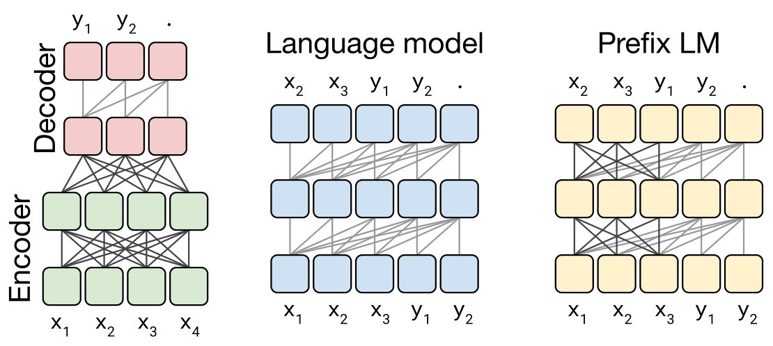
Figure 4: Schematics of the Transformer architecture variants we consider. In this diagram, blocks represent elements of a sequence and lines represent attention visibility. Different colored groups of blocks indicate different Transformer layer stacks. Dark grey lines correspond to fully-visible masking and light grey lines correspond to causal masking. We use “.” to denote a special end-of-sequence token that represents the end of a prediction. The input and output sequences are represented as and respectively. Left: A standard encoder-decoder architecture uses fully-visible masking in the encoder and the encoder-decoder attention, with causal masking in the decoder. Middle: A language model consists of a single Transformer layer stack and is fed the concatenation of the input and target, using a causal mask throughout. Right: Adding a prefix to a language model corresponds to allowing fully-visible masking over the input.
图4:我们考虑的Transformer结构变体的示意图. 在这个图中,块代表一个序列的元素,线代表注意的能见度. 不同颜色的块组表示不同的Transformer层堆栈. 暗灰色线对应全可见的遮盖,浅灰色线对应因果遮盖. 我们使用“.”来表示一种特殊的序列结束信号,它代表着预测的结束。 输入和输出序列分别以和表示. 左:一个标准的编码器-解码器架构在编码器和编码器-解码器的注意力中采用完全可见的遮罩,在解码器中带有因果遮罩. 中间:一种语言模型由单个Transformer层堆栈组成,并被输入和目标的调和,在整个过程中使用因果面具. 右:在语言模型中添加前缀对应允许在输入上完全可见的遮盖.
The first model structure we consider is an an encoder-decoder Transformer, which consists of two layer stacks: The encoder, which is fed an input sequence, and the decoder, which produces a new output sequence. A schematic of this architectural variant is shown in the left panel of Figure 4.
我们考虑的第一个模型结构是编码器-解码器Transformer,它由两层堆叠组成: 被输入序列的编码器和生成新输出序列的解码器. 该建筑变体的示意图见图4的左面板.
The encoder uses a “fully-visible” attention mask. Fully-visible masking allows a self-attention mechanism to attend to any entry of the input when producing each entry of its output. We visualize this masking pattern in Figure 3, left. This form of masking is appropriate when attending over a “prefix”, i.e. some context provided to the model that is later used when making predictions. BERT (Devlin et al. 2018) also uses a fully-visible masking pattern and appends a special “classification” token to the input. BERT’s output at the timestep corresponding to the classification token is then used to make a prediction for classifying the input sequence.
编码器使用“完全可见”的注意罩。 完全可见的遮罩可以使一个自觉机制在生产其输出的每个条目时能够处理输入的任何条目. 我们在图3中将这个蒙面图案描绘为左侧. 这种蒙面形式在“前缀”上,即向后来在预测时使用的模型提供某些上下文时是适当的。 BERT(Devlin等人,2018年)也使用全可见的遮盖图案,并在输入中附加一个特殊的"分类"符号. BERT在与分类符对应的时序输出,然后用于预测输入序列的分类.
The self-attention operations in the Transformer’s decoder use a “causal” masking pattern. When producing the th entry of the output sequence, causal masking prevents the model from attending to the th entry of the input sequence for . This is used during training so that the model can’t “see into the future” as it produces its output. An attention matrix for this masking pattern is shown in Figure 3, middle.
Transformer解码器中的自觉操作使用一种"因果"遮掩模式. 在生成输出序列的及其它输入序列的第2个条目时,因果遮罩使模型无法关注第2个输入序列的. 这在培训期间使用,以便模型在产生其产出时不能 " 看到未来 " 。 这种蒙面图案的注意矩阵如图3中所示.
The decoder in an encoder-decoder Transformer is used to autoregressively produce an output sequence. That is, at each output timestep, a token is sampled from the model’s predicted distribution and the sample is fed back into the model to produce a prediction for the next output timestep, and so on. As such, a Transformer decoder (without an encoder) can be used as a language model (LM), i.e. a model trained solely for next-step prediction (Liu et al. 2018; Radford et al. 2018; Al-Rfou et al. 2019). This constitutes the second model structure we consider. A schematic of this architecture is shown in Figure 4, middle. In fact, early work on transfer learning for NLP used this architecture with a language modeling objective as a pre-training method (Radford et al. 2018).
编码器-解码器Transformer中的解码器用于自动递归生成输出序列. 也就是说,在每个输出时间步上,从模型的预测分布中抽取一个符号,并将样本反馈到模型中,为下一个输出时间步作出预测等等. 因此,Transformer解码器(没有编码器)可以用作语言模型(LM),即完全为下一步预测而训练的模型(Liu等人,2018年;Radford等人,2018年;Al-Rfou等人,2019年). 这是我们认为的第二个模式结构。 这种建筑的图示如图4,中间部分所示. 事实上,NLP早期的转学学习工作将这个带有语言建模目标的架构作为预训方法(拉德福德等人,2018年).
Language models are typically used for compression or sequence generation (Graves 2013). However, they can also be used in the text-to-text framework simply by concatenating the inputs and targets. As an example, consider the case of English to German translation: If we have a training datapoint with input sentence “That is good.” and target “Das ist gut.”, we would simply train the model on next-step prediction over the concatenated input sequence “translate English to German: That is good. target: Das ist gut.” If we wanted to obtain the model’s prediction for this example, the model would be fed the prefix “translate English to German: That is good. target:” and would be asked to generate the remainder of the sequence autoregressively. In this way, the model can predict an output sequence given an input, which satisfies the needs of text-to-text tasks. This approach was recently used to show that language models can learn to perform some text-to-text tasks without supervision (Radford et al. 2019).
语言模型通常用于压缩或序列生成(Graves 2013). 然而,它们也可以仅仅通过压缩投入和目标在文本对文本框架中使用。 例如,将英文译为德文的情况: 如果我们有一个带有“很好”和“Das 这是很好的。 目标: " Das ist gut " 。 如果我们想获得模型的预测,这个模型会被输入前缀 " 将英语翻译成德语: 这是很好的。 目标:“并将要求自动生成序列的其余部分。 这样,模型可以预测给定输入的输出序列,这满足了文本到文本任务的需要. 这种方法最近被用来表明语言模型可以学会在没有监督的情况下执行一些文本对文本的任务(Radford等人,2019年).
A fundamental and frequently cited drawback of using a language model in the text-to-text setting is that causal masking forces the model’s representation of the th entry of the input sequence to only depend on the entries up until . To see why this is potentially disadvantageous, consider the text-to-text framework where the model is provided with a prefix/context before being asked to make predictions (e.g., the prefix is an English sentence and the model is asked to predict the German translation). With fully causal masking, the model’s representation of a prefix state can only depend on prior entries of the prefix. So, when predicting an entry of the output, the model will attend to a representation of the prefix that is unnecessarily limited. Similar arguments have been made against using a unidirectional recurrent neural network encoder in sequence-to-sequence models (Bahdanau et al. 2015).
在文本对文本设置中使用一种语言模型的一个基本和经常提到的缺点是,因果遮掩迫使该模型代表输入序列的第2个条目,只取决于直到为止的条目。 为了了解这有潜在劣势的原因,在被要求作出预测(例如前缀是英文句子,要求模型预测德文翻译)之前,先考虑给模型提供前缀/语句的文本对文本框架. 在完全因果遮盖的情况下,模型对前缀状态的表示只能取决于前缀的先前条目. 因此,在预测输出的条目时,模型将处理一个不必要限制的前缀的表示. 也有人提出类似的论点,反对在序列到序列模型中使用单向反复神经网络编码器(Bahdanau等人,2015年)。
This issue can be avoided in a Transformer-based language model simply by changing the masking pattern. Instead of using a causal mask, we use fully-visible masking during the prefix portion of the sequence. This masking pattern and a schematic of the resulting “prefix LM” (the third model structure we consider) are illustrated in the rightmost panels of Figures 3 and 4, respectively. In the English to German translation example mentioned above, fully-visible masking would be applied to the prefix “translate English to German: That is good. target:” and causal masking would be used during training for predicting the target “Das ist gut.” Using a prefix LM in the text-to-text framework was originally proposed by Liu et al. 2018. More recently, Dong et al. 2019 showed that this architecture is effective on a wide variety of text-to-text tasks. This architecture is similar to an encoder-decoder model with parameters shared across the encoder and decoder and with the encoder-decoder attention replaced with full attention across the input and target sequence.
这个问题可以在基于Transformer的语言模型中简单地通过改变遮掩模式来避免. 与其使用因果口罩,不如在序列的前缀部分使用全可见口罩. 图3和图4最右侧的板块分别说明了这种掩盖模式和由此产生的“前缀LM”(我们认为是第三个模型结构)。 在上文提到的英文到德文翻译例子中,完全可见的面具将适用于前缀“将英文译为德文: 这是很好的。 目标:“和因果遮罩将用于训练,以预测目标“Das ist gut”。 在文本对文本框架中使用前缀LM最初是由刘等人在2018年提出的. 最近,董等人的2019年显示,这种架构在各种各样的文本对文本任务上是有效的. 这种架构类似于一个编码器-解码器模型,其参数在编码器和解码器之间共享,而编码器-解码器的注意力则在输入和目标序列之间被完全的注意所取代.
We note that when following our text-to-text framework, the prefix LM architecture closely resembles BERT (Devlin et al. 2018) for classification tasks. To see why, consider an example from the MNLI benchmark where the premise is “I hate pigeons.”, the hypothesis is “My feelings towards pigeons are filled with animosity.” and the correct label is “entailment”. To feed this example into a language model, we would transform it into the sequence “mnli premise: I hate pigeons. hypothesis: My feelings towards pigeons are filled with animosity. target: entailment”. In this case, the fully-visible prefix would correspond to the entire input sequence up to the word “target:”, which can be seen as being analogous to the “classification” token used in BERT. So, our model would have full visibility over the entire input, and then would be tasked with making a classification by outputting the word “entailment”. It is easy for the model to learn to output one of the valid class labels given the task prefix (“mnli” in this case). As such, the main difference between a prefix LM and the BERT architecture is that the classifier is simply integrated into the output layer of the Transformer decoder in the prefix LM.
我们注意到,在遵循我们的文本对文本框架时,前缀LM架构与分类任务的BERT(Devlin等人,2018年)非常相似. 为了了解原因,请从MNLI基准中以“我讨厌鸽子”为前提,假设是“我对鸽子的感情充满敌意”。 为了将这个例子输入语言模型,我们将把它变成“mnli前提:我讨厌鸽子”。 假设:我对鸽子的感情充满敌意. 目标:产生”。 在这种情况下,完全可见的前缀将对应整个输入序列,直至“目标:”一词,这可被视为类似于BERT中使用的“分类”符号。 因此,我们的模型将对整个投入具有充分的可见度,然后负责通过输出“尾注”一词来进行分类。 模型很容易在任务前缀(在此情况下为“mnli”)中学习输出一个有效的类标签。 因此,前缀LM和BERT架构的主要区别在于,分类器只是被整合到前缀LM中的Transformer解码器的输出层中.
3.2.2 Comparing Different Model Structures
In the interest of experimentally comparing these architectural variants, we would like each model we consider to be equivalent in some meaningful way. We might say that two models are equivalent if they either have the same number of parameters or they require roughly the same amount of computation to process a given (input-sequence, target-sequence) pair. Unfortunately, it is not possible to compare an encoder-decoder model to a language model architecture (comprising a single Transformer stack) according to both of these criteria at the same time. To see why, first note an encoder-decoder model with layers in the encoder and layers in the decoder has approximately the same number of parameters as a language model with layers. However, the same encoder-decoder model will have approximately the same computational cost as a language model with only layers. This is a consequence of the fact that the layers in the language model must be applied to both the input and output sequence, while the encoder is only applied to the input sequence and the decoder is only applied to the output sequence. Note that these equivalences are approximate—there are some extra parameters in the decoder due to the encoder-decoder attention and there are also some computational costs in the attention layers that are quadratic in the sequence lengths. In practice, however, we observed nearly identical step times for -layer language models versus -layer encoder-decoder models, suggesting a roughly equivalent computational cost. Further, for the model sizes we consider, the number of parameters in the encoder-decoder attention layers is about 10% of the total parameter count, so we make the simplifying assumption that an -layer encoder-decoder model has the same number of parameters as an -layer language model.
3.2.2 比较不同的模型结构
为了实验性地比较这些建筑变体,我们希望我们所认为的每一个模型都以某种有意义的方式等同起来. 我们可以说,如果两个模型的参数数目相同,或者它们需要大致相同的计算量来处理一个给定的对(输入-序列,目标-序列),这两个模型是等效的. 不幸的是,无法同时根据这两个标准将编码器-解码器模型与语言模型架构(包含一个单Transformer堆栈)进行比较. 要了解为什么,首先注意一个编码器-解码器模型,其编码器中的层和解码器中的层的参数数量与具有层的语言模型大致相同. 然而,同样的编码器-解码器模型的计算成本与语言模型大致相同,只有**层. 这是由于语言模型中的层必须应用于*双 *输入和输出序列,而编码器仅适用于输入序列,解码器仅适用于输出序列. 注意这些等效物是近似的——由于编码器-解码器的注意,解码器中有一些额外的参数,在注意层中也有一些计算成本,在序列长度上是四极的. 然而,在实践中,我们看到-层语言模型与-层编码器-解码器模型的步数几乎相同,表明计算成本大致相当。 此外,对于我们考虑的模型大小,编码器-解码器关注层中的参数数大约是总参数数的10%,所以我们做了简化的假设,即-层编码器-解码器模型的参数数与-层语言模型相同.
To provide a reasonable means of comparison, we consider multiple configurations for our encoder-decoder model. We will refer to the number of layers and parameters in a BERTBASE-sized layer stack as and , respectively. We will use to refer to the number of FLOPs required for an -layer encoder-decoder model or -layer decoder-only model to process a given input-target pair. In total, we will compare:
为了提供合理的比较手段,我们考虑我们的编码器-解码器模型的多种配置. 我们将分别以和来指代BERTBASE大小的层堆栈中的层数和参数. 我们将使用来指代一个 - 层编码器-解码器模型或 - 层解码器-只处理一个给定输入目标对所需的FLOP数量. 总的来说,我们将比较:
- • An encoder-decoder model with layers in the encoder and layers in the decoder. This model has parameters and a computation cost of FLOPs.
- • An equivalent model, but with parameters shared across the encoder and decoder, resulting in parameters and an -FLOP computational cost.
- • An encoder-decoder model with layers each in the encoder and decoder, giving parameters and an -FLOP cost.
- • A decoder-only language model with layers and parameters and a resulting computational cost of FLOPs.
- • A decoder-only prefix LM with the same architecture (and thus the same number of parameters and computational cost), but with fully-visible self-attention over the input.
- 编码器-解码器模型,其中编码器为层,解码器为层。 该模型有参数和 FLOP的计算成本.
- 等效模型,但参数在编码器和解码器之间共享,导致参数和-FLOP计算成本。
- 一个编码器-解码器模型,在编码器和解码器中各有层,给出参数和-FLOP成本.
- 一个只有解码器的语言模型,有层和参数,并由此产生 FLOP的计算成本.
- 只有一个解码器的前缀LM,其结构相同(因此参数和计算成本相同),但在输入上完全可见。
3.2.3 Objectives
As an unsupervised objective, we will consider both a basic language modeling objective as well as our baseline denoising objective described in Section 3.1.4. We include the language modeling objective due to its historic use as a pre-training objective (Dai and Le 2015; Ramachandran et al. 2016; Howard and Ruder 2018; Radford et al. 2018; Peters et al. 2018) as well as its natural fit for the language model architectures we consider. For models that ingest a prefix before making predictions (the encoder-decoder model and prefix LM), we sample a span of text from our unlabeled data set and choose a random point to split it into prefix and target portions. For the standard language model, we train the model to predict the entire span from beginning to end. Our unsupervised denoising objective is designed for text-to-text models; to adapt it for use with a language model we concatenate the inputs and targets as described in Section 3.2.1.
3.2.3 目标
作为一项不受监督的目标,我们将既考虑基本的语文建模目标,也考虑第3.1.4节所述的基线去名目标。 我们包括了语言建模目标,因为其作为培训前目标的历史用途(Dai和Le 2015;Ramachandran等人,2016年;Howard和Ruder 2018;Radford等人,2018年;Peters等人,2018年)及其与我们认为的语言建模架构的自然适合性. 对于在作出预测前摄入前缀的模型(编码器-解码器模型和前缀LM),我们从我们无标签的数据集中抽取了一段文字,并选择随机点将其分为前缀和目标部分. 对于标准语言模型,我们训练模型来预测从开始到结束的整个跨度. 我们不受监督的去名目标是为文本对文本模式设计的;为了使其与语言模式相适应,我们将第3.2.1节所述的投入和目标结合起来。
3.2.4 Results
| Architecture | Objective | Params | Cost | GLUE | CNNDM | SQuAD | SGLUE | EnDe | EnFr | EnRo |
|---|---|---|---|---|---|---|---|---|---|---|
| Encoder-decoder | Denoising | |||||||||
| Enc-dec, shared | Denoising | |||||||||
| Enc-dec, 6 layers | Denoising | |||||||||
| Language model | Denoising | |||||||||
| Prefix LM | Denoising | |||||||||
| Encoder-decoder | LM | |||||||||
| Enc-dec, shared | LM | |||||||||
| Enc-dec, 6 layers | LM | |||||||||
| Language model | LM | |||||||||
| Prefix LM | LM |
Table 2: Performance of the different architectural variants described in Section 3.2.2. We use to refer to the number of parameters in a 12-layer base Transformer layer stack and to refer to the FLOPs required to process a sequence using the encoder-decoder model. We evaluate each architectural variant using a denoising objective (described in Section 3.1.4) and an autoregressive objective (as is commonly used to train language models).
3.2.4 结果煞费苦心
EnFr = EnRo ===
唵(引)|日啰(二合引)贺(引)贺.
Encoder-decoder
XXMAT的三个月
语言模型
LM
LM 前缀 LM
表2:第3.2.2节所述不同建筑变体的性能。 我们使用来指代一个12层基底Transformer层堆栈中的参数数,而来指代使用编码器-解码器模型处理一个序列所需的FLOP. 我们使用一个去名目标(在第3.1.4节中描述)和一个自动递归目标(通常用于培训语言模型)来评价每个建筑变体。
The scores achieved by each of the architectures we compare are shown in Table 2. For all tasks, the encoder-decoder architecture with the denoising objective performed best. This variant has the highest parameter count () but the same computational cost as the -parameter decoder-only models. Surprisingly, we found that sharing parameters across the encoder and decoder performed nearly as well. In contrast, halving the number of layers in the encoder and decoder stacks significantly hurt performance. Concurrent work (Lan et al. 2019) also found that sharing parameters across Transformer blocks can be an effective means of lowering the total parameter count without sacrificing much performance. XLNet also bears some resemblance to the shared encoder-decoder approach with a denoising objective (Yang et al. 2019). We also note that the shared parameter encoder-decoder outperforms the decoder-only prefix LM, suggesting that the addition of an explicit encoder-decoder attention is beneficial. Finally, we confirm the widely-held conception that using a denoising objective always results in better downstream task performance compared to a language modeling objective. This observation has been previously made by Devlin et al. 2018, Voita et al. 2019, and Lample and Conneau 2019 among others. We undertake a more detailed exploration of unsupervised objectives in the following section.
我们所比较的每个架构所获得的分数见表2。 对所有任务来说,带有解密目标的编码器-解码器架构表现最好. 此变体拥有最高参数计数(),但与-参数解码器唯一模式的计算成本相同. 令人惊讶的是,我们发现共享参数 跨编码器和解码器几乎也完成了。 相比之下,将编码器和解码器堆栈的层数减半,对性能有很大的伤害. 同时期工作(Lan et al. 2019)也发现跨变形星块共享参数可以成为降低总参数计数而不牺牲很多性能的有效手段. XLNet也与具有去诺目标的共同编码器-解码器方法有些相似(Yang等人,2019年). 我们还注意到,共享参数编码器-解码器超越了解码器唯一的前缀LM,建议添加一个明确的编码器-解码器的注意是有好处的. 最后,我们确认一个普遍持有的概念,即使用去名目标总是比语言建模目标更能完成下游任务。 此观测此前由Devlin等人2018年,Voita等人2019年,Lample和Conneau2019等人提出. 我们将在下一节更详细地探讨不受监督的目标。
3.3 Unsupervised Objectives
3.3 无监督目标
The choice of unsupervised objective is of central importance as it provides the mechanism through which the model gains general-purpose knowledge to apply to downstream tasks. This has led to the development of a wide variety of pre-training objectives (Dai and Le 2015; Ramachandran et al. 2016; Radford et al. 2018; Devlin et al. 2018; Yang et al. 2019; Liu et al. 2019b; Wang et al. 2019a; Song et al. 2019; Dong et al. 2019; Joshi et al. 2019). In this section, we perform a procedural exploration of the space of unsupervised objectives. In many cases, we will not replicate an existing objective exactly—some will be modified to fit our text-to-text encoder-decoder framework and, in other cases, we will use objectives that combine concepts from multiple common approaches.
选择不受监督的目标至关重要,因为它提供了一种机制,通过这一机制,该模式获得普通用途知识,用于下游任务。 这导致了各种培训前目标的发展(Dai和Le 2015;Ramachandran等人,2016年;Radford等人,2018年;Devlin等人,2018年;Yang等人,2019年;Liu等人,2019年b;Wang等人,2019年a;Song等人,2019年;Dong等人,2019年;Dong等人,2019年9月20日;Dong等人,2019年9月20日;Devford等人,2018年;Devlin等人,2018年;Yang等人,2019年9月20日;Liu等人,2019年b;Wang等人,2019年a;Song等人,2019年19年;Dong等人,2019年9月2019日;Dong等人,2019年1月2019日)。 在本节中,我们从程序上探讨不受监督的目标的空间。 在许多情况下,我们不会完全照搬一个现有目标——有些目标将加以修改,以适应我们从文本到文本的编码器-解码器框架,而在另一些情况下,我们将使用从多种共同办法中综合概念的目标。
Overall, all of our objectives ingest a sequence of token IDs corresponding to a tokenized span of text from our unlabeled text data set. The token sequence is processed to produce a (corrupted) input sequence and a corresponding target. Then, the model is trained as usual with maximum likelihood to predict the target sequence. We provide illustrative examples of many of the objectives we consider in Table 3.
总的来说,我们所有的目标 都摄取了一系列的代号标识 与我们未加标签的文本数据集的代号长度相对应 符号序列经过处理,生成一个(被腐蚀)输入序列和相应的目标. 之后,该模型被照常训练,最有可能预测目标序列. 我们举例说明了我们在表3中考虑的许多目标。
| Objective | Inputs | Targets |
|---|---|---|
| Prefix language modeling | Thank you for inviting | me to your party last week . |
| BERT-style Devlin et al. 2018 | Thank you me to your party apple week . | (original text) |
| Deshuffling | party me for your to . last fun you inviting week Thank | (original text) |
| MASS-style Song et al. 2019 | Thank you me to your party week . | (original text) |
| I.i.d. noise, replace spans | Thank you me to your party week . | for inviting last |
| I.i.d. noise, drop tokens | Thank you me to your party week . | for inviting last |
| Random spans | Thank you to week . | for inviting me your party last |
Table 3: Examples of inputs and targets produced by some of the unsupervised objectives we consider applied to the input text “Thank you for inviting me to your party last week .” Note that all of our objectives process tokenized text. For this particular sentence, all words were mapped to a single token by our vocabulary. We write (original text) as a target to denote that the model is tasked with reconstructing the entire input text. denotes a shared mask token and , , and denote sentinel tokens that are assigned unique token IDs. The BERT-style objective (second row) includes a corruption where some tokens are replaced by a random token ID; we show this via the greyed-out word apple.
| 目标 | 输入 | 目标 |
|---|---|---|
| 前缀语言建模 | 谢谢你的邀请 | 我上周参加你的派对 |
| BERT风格Devlin等人 2018年 | 感谢您"M" "M" 我为您的派对苹果周。 | (原文) |
| 脱衣舞 | 请你为我狂欢吧,最后的乐趣 | 践行(原文) |
| MASS风格的宋等 2019 | 感谢你的"M" "M" 我对你的"M"周。 | (原文) |
| I.i.d. 噪声,替换跨度 | 谢谢你的派对 "Y"周。 | QQ 用于邀请 最后一个 |
| I.i.d. 噪声, 投币 | 谢谢你的派对周。 | 用于最后一次邀请 |
| 随机跨度 | 感谢您 我不想在"Y"周。 | QQ 因邀请我 "Y " 您的晚会最后一次"Z" |
表3:一些未经监督的目标所产生的投入和目标的例子,我们认为这些投入适用于“感谢你上周邀请我参加你的聚会”。 请注意,我们的所有目标都经过了kenized文本。 对于这个特别的句子,所有词都用我们的词汇图成一个符号. 我们写 * (原始文本) * 作为目标,以表示该模型的任务是重建整个输入文本。 表示一个共享的掩码, +, , 表示被指定为唯一代号的哨点标识。 BERT风格的目标(第二行)包括一种腐败,即一些令牌被随机令牌ID所取代;我们通过灰外字苹果来显示这一点.
3.3.1 Disparate High-Level Approaches
To begin with, we compare three techniques that are inspired by commonly-used objectives but differ significantly in their approach. First, we include a basic “prefix language modeling” objective as was used in Section 3.2.3. This technique splits a span of text into two components, one to use as inputs to the encoder and the other to use as a target sequence to be predicted by the decoder. Second, we consider an objective inspired by the “masked language modeling” (MLM) objective used in BERT (Devlin et al. 2018). MLM takes a span of text and corrupts of the tokens. of the corrupted tokens are replaced with a special mask token and are replaced with a random token. Since BERT is an encoder-only model, its goal during pre-training is to reconstruct masked tokens at the output of the encoder. In the encoder-decoder case, we simply use the entire uncorrupted sequence as the target. Note that this differs from our baseline objective, which uses only the corrupted tokens as targets; we compare these two approaches in Section 3.3.2. Finally, we also consider a basic deshuffling objective as used e.g. in (Liu et al. 2019a) where it was applied to a denoising sequential autoencoder. This approach takes a sequence of tokens, shuffles it, and then uses the original deshuffled sequence as a target. We provide examples of the inputs and targets for these three methods in the first three rows of Table 3.
3.3.1 不同高级别办法
首先,我们比较了三种技术,它们受常用目标的启发,但其方法差别很大。 首先,我们列入了第3.2.3节中使用的基本“前缀语文模式”目标。 这一技术将一段文字分成两个部分,一个是用作编码器的输入,另一个是用作解码器预测的目标序列. 其次,我们认为一个目标受到BERT(Devlin等人,2018年)中使用的“假冒语言建模”(MLM)目标的启发。 MLM需要一段文字,并损坏了符号的. 被腐蚀的代币的被替换为特殊的面具代币,被替换为随机代币. 由于BERT是一个只编码器的模型,它在预训期间的目标是在编码器输出时重建蒙面符号. 在编码器-解码器的情况下,我们只是使用整个未腐蚀的序列作为目标. 请注意,这与我们的基线目标不同,因为基线目标只使用腐败的标志作为目标;我们在第3.3.2节中比较了这两种方法。 最后,我们也考虑在制定一个基本解析目标,例如(Liu等人,2019年a)中,它被应用到自动编码器中。 这种方法采用一系列的符号,洗牌,然后使用原来的解牌序列作为目标. 我们举例说明表3前三行对这三种方法的投入和目标。
| Objective | GLUE | CNNDM | SQuAD | SGLUE | EnDe | EnFr | EnRo |
|---|---|---|---|---|---|---|---|
| Prefix language modeling | |||||||
| BERT-style (Devlin et al. 2018) | |||||||
| Deshuffling |
Table 4: Performance of the three disparate pre-training objectives described in Section 3.3.1.
| 目标 | 格吕 | CNNDM( CNNDM ) : 美国主题 美国主题 美国主题 美国主题 美国主题 美国主题 美国主题 | SQAD 状态 | 英格兰 | 定义 | 定义Fr | 安围绕着 |
|---|---|---|---|---|---|---|---|
| 前缀语言建模 | |||||||
| BERT风格(Devlin等人,2018年). | |||||||
| 脱衣舞 |
表 Rainbow4:第3.3.1节所述三个不同的培训前目标的执行情况。
The performance of these three objectives is shown in Table 4. Overall, we find that the BERT-style objective performs best, though the prefix language modeling objective attains similar performance on the translation tasks. Indeed, the motivation for the BERT objective was to outperform language model-based pre-training. The deshuffling objective performs considerably worse than both prefix language modeling and the BERT-style objective.
这三个目标的执行情况见表4。 总的来说,我们发现BERT式的目标表现最好,尽管前缀语言模型的目标在翻译任务上也取得了类似的表现. 事实上,BERT目标的动机是超越基于语言模式的预训。 拆解目标的表现比前缀语言模型和BERT风格的目标都差得多.
3.3.2 Simplifying the BERT Objective
Based on the results in the prior section, we will now focus on exploring modifications to the BERT-style denoising objective. This objective was originally proposed as a pre-training technique for an encoder-only model trained for classification and span prediction. As such, it may be possible to modify it so that it performs better or is more efficient in our encoder-decoder text-to-text setup.
3.3.2 简化BERT目标
根据上一节中的结果,我们现在将集中探讨修改BERT式的去名目标。 这一目标最初是作为培训前技术提出的,用于一种只经过分类和跨度预测培训的编码器模型。 因此,也许可以修改它,以便在我们的编码器-解码器文本到文本设置中更好地或更有效地执行它.
First, we consider a simple variant of the BERT-style objective where we don’t include the random token swapping step. The resulting objective simply replaces of the tokens in the input with a mask token and the model is trained to reconstruct the original uncorrupted sequence. A similar masking objective was used by Song et al. 2019 where it was referred to as “MASS”, so we call this variant the “MASS-style” objective. Second, we were interested to see if it was possible to avoid predicting the entire uncorrupted text span since this requires self-attention over long sequences in the decoder. We consider two strategies to achieve this: First, instead of replacing each corrupted token with a mask token, we replace the entirety of each consecutive span of corrupted tokens with a unique mask token. Then, the target sequence becomes the concatenation of the “corrupted” spans, each prefixed by the mask token used to replace it in the input. This is the pre-training objective we use in our baseline, described in Section 3.1.4. Second, we also consider a variant where we simply drop the corrupted tokens from the input sequence completely and task the model with reconstructing the dropped tokens in order. Examples of these approaches are shown in the fifth and sixth rows of Table 3.
首先,我们考虑BERT式目标的一个简单变体,我们并不包括随机代币互换步骤。 由此产生的目标只是将输入中的符号的替换成一个面具符号,模型被训练来重建原始的未腐蚀序列. Song et al. 2019使用了类似的遮掩目标,它被称为“MASS”,因此,我们称这个变体为“MASS风格”目标。 第二,我们想了解是否能够避免预测整个未腐蚀文本的跨度,因为这需要自己注意解码器中的长序列。 我们考虑两种策略来达到这个目的:第一,我们不是用面具标志取代每一个腐烂的标志,而是用一个独特的面具标志来取代每一个连续的腐烂标志的全部. 然后,目标序列成为“腐蚀”跨度的调和,每个跨度的前缀都是用于替换输入中的面具符号。 这是我们在第3.1.4节所述基线中采用的训练前目标。 其次,我们也考虑一种变体,我们简单地从输入序列中完全放下腐烂的符号,并让模型按照顺序重建掉的符号. 这些方法的例子见表3第五和第六行。
| Objective | GLUE | CNNDM | SQuAD | SGLUE | EnDe | EnFr | EnRo |
|---|---|---|---|---|---|---|---|
| BERT-style (Devlin et al. 2018) | |||||||
| MASS-style (Song et al. 2019) | |||||||
| Replace corrupted spans | |||||||
| Drop corrupted tokens |
Table 5: Comparison of variants of the BERT-style pre-training objective. In the first two variants, the model is trained to reconstruct the original uncorrupted text segment. In the latter two, the model only predicts the sequence of corrupted tokens.
| 目标 | 格 当我们是... | CNNDM( CNNDM ) : 美国主题 美国主题 美国主题 美国主题 美国主题 美国主题 美国主题 | SQAD 状态 | 英格兰 | 定义 | 定义Fr | 恩罗 |
|---|---|---|---|---|---|---|---|
| BERT风格(Devlin等人,2018年). | |||||||
| MASS型(宋等人,2019年) | |||||||
| 第二十届 替换已损坏的跨度 | |||||||
| 丢弃已损坏的令牌 |
表5:BERT式预训目标的变种比较. 在前两个变体中,该模型被训练来重建原始的未腐蚀文本段. 在后两者中,模型只预测腐烂的符的序列.
An empirical comparison of the original BERT-style objective to these three alternatives is shown in Table 5. We find that in our setting, all of these variants perform similarly. The only exception was that dropping corrupted tokens completely produced a small improvement in the GLUE score thanks to a significantly higher score on CoLA (, compared to our baseline average of , see Table 16). This may be due to the fact that CoLA involves classifying whether a given sentence is grammatically and syntactically acceptable, and being able to determine when tokens are missing is closely related to detecting acceptability. However, dropping tokens completely performed worse than replacing them with sentinel tokens on SuperGLUE. The two variants that do not require predicting the full original sequence (“replace corrupted spans” and “drop corrupted spans”) are both potentially attractive since they make the target sequences shorter and consequently make training faster. Going forward, we will explore variants where we replace corrupted spans with sentinel tokens and only predict the corrupted tokens (as in our baseline objective).
表5对最初的BERT式目标与这三种选择进行了实证比较。 我们发现,在我们所处的环境里,所有这些变体都表现得相似。 唯一的例外是,由于COLA的得分明显较高,降下腐烂的代币完全导致GLUE分数略有改善(,与我们的基线平均值相比,见表16)。 这可能是因为CoLA涉及对某一句子在语法上和在战术上是否可接受进行分类,并且能够确定是否缺少符号与检测可接受性密切相关. 然而,投放令牌的表现完全不如SuperGLUE上的哨兵令牌取代. 不需要预测全部原始序列的两个变体(“替换腐败的跨度”和“下降腐败的跨度”)都具有潜在吸引力,因为这些变体使目标序列缩短,从而使培训更快。 展望未来,我们将探索各种变体,在其中我们用监控符代替腐败的跨度,并且只预测腐败的标志(如我们的基线目标).
3.3.3 Varying the Corruption Rate
So far, we have been corrupting 15% of the tokens, the value used in BERT (Devlin et al. 2018). Again, since our text-to-text framework differs from BERT’s, we are interested to see if a different corruption rate works better for us. We compare corruption rates of , , , and in Table 6. Overall, we find that the corruption rate had a limited effect on the model’s performance. The only exception is that the largest corruption rate we consider () results in a significant degradation of performance on GLUE and SQuAD. Using a larger corruption rate also results in longer targets, which can potentially slow down training. Based on these results and the historical precedent set by BERT, we will use a corruption rate of going forward.
3.3.3 腐败率的变化
目前为止,我们一直在腐蚀15%的代币,BERT中使用的值(Devlin等人,2018年). 我们想知道不同的腐败率对我们是否更好。 我们比较表6中的、、和的腐败率。 总体来说,我们发现腐败率对模型的性能影响有限。 唯一的例外是,我们认为最大的腐败率()导致GLUE和SQuAD的业绩严重下降。 使用较高的腐败率也会导致目标更长,这有可能减缓培训。 根据这些结果和BERT开创的历史先例,我们将使用的腐败率向前迈进。
| Corruption rate | GLUE | CNNDM | SQuAD | SGLUE | EnDe | EnFr | EnRo |
|---|---|---|---|---|---|---|---|
Table 6: Performance of the i.i.d. corruption objective with different corruption rates.
| 腐败率 | 格吕 | CNNDM( CNNDM ) : 美国主题 美国主题 美国主题 美国主题 美国主题 美国主题 美国主题 | SQAD 状态 | 英格兰 | 定义 | 定义Fr | 恩罗 |
|---|---|---|---|---|---|---|---|
表6:不同腐败率的腐败目标的业绩。
3.3.4 Corrupting Spans
We now turn towards the goal of speeding up training by predicting shorter targets. The approach we have used so far makes an i.i.d. decision for each input token as to whether to corrupt it or not. When multiple consecutive tokens have been corrupted, they are treated as a “span” and a single unique mask token is used to replace the entire span. Replacing entire spans with a single token results in unlabeled text data being processed into shorter sequences. Since we are using an i.i.d. corruption strategy, it is not always the case that a significant number of corrupted tokens appear consecutively. As a result, we might obtain additional speedup by specifically corrupting spans of tokens rather than corrupting individual tokens in an i.i.d. manner. Corrupting spans was also previously considered as a pre-training objective for BERT, where it was found to improve performance (Joshi et al. 2019).
3.3.4 腐蚀西班牙人
我们现在通过预测更短的目标来实现加快培训的目标。 我们迄今采用的方法使每个输入符号都能够就是否腐败问题作出决定。 当多个连续的符号被损坏时,它们被当作一个“span”处理,并使用一个单一的独特面具符号来取代整个长度。 以单个符号取代整个跨度,导致未加标签的文本数据被处理成较短的序列。 因为我们正在采用 " i.d. " 的腐败策略,并非总能连续出现大量腐败的标志。 因此,我们可能会通过具体腐蚀象征物的跨度而获得额外的加速,而不是以某种方式腐蚀个别象征物。 腐败期以前也被认为是BERT的培训前目标,在那里发现它可以提高性能(Joshi等人,2019年).
To test this idea, we consider an objective that specifically corrupts contiguous, randomly-spaced spans of tokens. This objective can be parametrized by the proportion of tokens to be corrupted and the total number of corrupted spans. The span lengths are then chosen randomly to satisfy these specified parameters. For example, if we are processing a sequence of tokens and we have specified that of tokens should be corrupted and that there should be total spans, then the total number of corrupted tokens would be and the average span length would be . Note that given the original sequence length and corruption rate, we can equivalently parametrize this objective either by the average span length or the total number of spans.
为了检验这个想法,我们考虑一个目标,它具体地腐蚀了毗连的,随机间隔的代币. 这一目标可以被破坏的代币比例和腐败的跨度总数所压倒. 然后随机选择长度来满足这些指定的参数. 例如,如果我们正在处理一个令牌的序列,而且我们已经规定令牌应当被损坏,并且应该有总跨度,那么被损坏令牌的总数将是 ,平均跨度将是。 请注意,鉴于最初的序列长度和腐败率,我们可以以平均长度或总长度等同地使这一目标瘫痪。
| Span length | GLUE | CNNDM | SQuAD | SGLUE | EnDe | EnFr | EnRo |
|---|---|---|---|---|---|---|---|
| Baseline (i.i.d.) | |||||||
Table 7: Performance of the span-corruption objective (inspired by Joshi et al. 2019) for different average span lengths. In all cases, we corrupt 15% of the original text sequence.
| 宽度 | 格吕 | CNNDM( CNNDM ) : 美国主题 美国主题 美国主题 美国主题 美国主题 美国主题 美国主题 | SQAD 状态 | 英格兰 | 定义 | 定义Fr | 恩罗 |
|---|---|---|---|---|---|---|---|
| 基线(一.d.) | |||||||
表7:跨度腐败目标(Joshi等人,2019年)不同平均跨度的绩效。 在所有情况下,我们腐败了15%的原始文本序列.
We compare the span-corruption objective to the i.i.d-corruption objective in Table 7. We use a corruption rate of in all cases and compare using average span lengths of , , and . Again, we find a limited difference between these objectives, though the version with an average span length of slightly underperforms the other values in some cases. We also find in particular that using an average span length of slightly (but significantly) outperforms the i.i.d. objective on most non-translation benchmarks. Fortunately, the span-corruption objective also provides some speedup during training compared to the i.i.d. noise approach because span corruption produces shorter sequences on average.
我们比较了表7中的跨腐败目标与即腐败目标。 我们在所有案件中都采用的腐败率,并使用XX墅道1XX、、和的平均长度进行比较。 我们再次发现,这些目标之间的差别有限,尽管平均跨度为的版本在某些情况下略低于其他数值。 我们还特别发现,使用的平均跨度略微(但显著)超过大多数非翻译基准的目标。 所幸的是,在培训期间,跨度腐败目标也比 " 噪音 " 方法提供了一些速度,因为跨度腐败平均产生较短的序列。
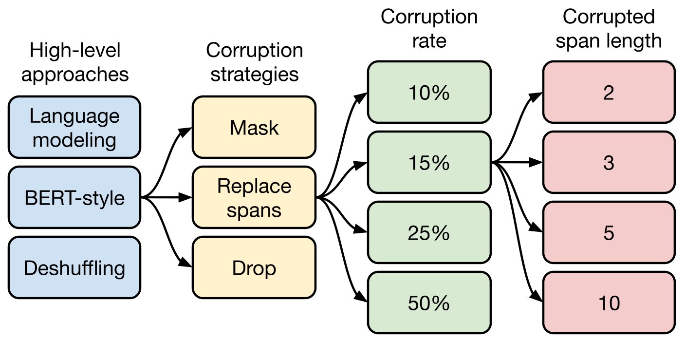
Figure 5: A flow chart of our exploration of unsupervised objectives. We first consider a few disparate approaches in Section 3.3.1 and find that a BERT-style denoising objective performs best. Then, we consider various methods for simplifying the BERT objective so that it produces shorter target sequences in Section 3.3.2. Given that replacing dropped-out spans with sentinel tokens performs well and results in short target sequences, in Section 3.3.3 we experiment with different corruption rates. Finally, we evaluate an objective that intentionally corrupts contiguous spans of tokens in Section 3.3.4.
图5:我们探索无监督目标的流程图. 我们首先在第3.3.1节中考虑了几种不同的做法,认为BERT式的去名化目标最能发挥效用。 然后,我们考虑简化BERT目标的各种方法,以便它在第3.3.2节产生较短的目标序列。 鉴于以哨兵代号取代退学的期间表现良好,结果目标序列短,在第3.3节中,我们试验了不同的腐败率。 最后,我们评价第3.3.4节中故意破坏毗连的标志范围的目标。
3.3.5 Discussion
Figure 5 shows a flow chart of the choices made during our exploration of unsupervised objectives. Overall, the most significant difference in performance we observed was that denoising objectives outperformed language modeling and deshuffling for pre-training. We did not observe a remarkable difference across the many variants of the denoising objectives we explored. However, different objectives (or parameterizations of objectives) can lead to different sequence lengths and thus different training speeds. This implies that choosing among the denoising objectives we considered here should mainly be done according to their computational cost. Our results also suggest that additional exploration of objectives similar to the ones we consider here may not lead to significant gains for the tasks and model we consider. Instead, it may be fortuitous to explore entirely different ways of leveraging unlabeled data.
3.3.5 讨论
图5显示了我们探索无监督目标期间所作的选择流程图。 人所共知, 人所共知。 我们没有看到我们所探讨的诽谤目标的许多变体之间有显著的差异。 然而,不同的目标(或目标参数化)可能导致不同的序列长度,从而导致不同的训练速度. 这意味着,在本文所考虑的取消提名目标中作出选择应主要根据其计算成本进行。 我们的结果还表明,进一步探讨与我们在这里审议的目标相似的目标,可能不会使我们审议的任务和模式取得重大进展。 相反,探索利用无标签数据的完全不同的方法可能是偶然的。
3.4 Pre-training Data set
3.4 预训练数据集
Like the unsupervised objective, the pre-training data set itself is a crucial component of the transfer learning pipeline. However, unlike objectives and benchmarks, new pre-training data sets are usually not treated as significant contributions on their own and are often not released alongside pre-trained models and code. Instead, they are typically introduced in the course of presenting a new method or model. As a result, there has been relatively little comparison of different pre-training data sets as well as a lack of a “standard” data set used for pre-training. Some recent notable exceptions (Baevski et al. 2019; Liu et al. 2019c; Yang et al. 2019) have compared pre-training on a new large (often Common Crawl-sourced) data set to using a smaller preexisting data set (often Wikipedia). To probe more deeply into the impact of the pre-training data set on performance, in this section we compare variants of our C4 data set and other potential sources of pre-training data. We release all of the C4 data set variants we consider as part of TensorFlow Datasets.[^11]
与未受监督的目标一样,培训前数据集本身也是转移学习程序的重要组成部分。 然而,与目标和基准不同的是,新的培训前数据集通常不单独作为重大贡献对待,而且往往不与培训前的模型和代码一起发布。 相反,它们通常是在提出新方法或模式的过程中提出的。 因此,不同的培训前数据集比较较少,而且缺乏用于培训前的“标准”数据集。 最近一些显著的例外(Baevski等人,2019年;Liu等人,2019年c;Yang等人,2019年)将新大型(常为常见的爬行源)数据集的预训比作使用更小的原有数据集(常为维基百科). 为了更深入地探索培训前数据集对性能的影响,我们在本节中比较了我们的C4数据集的变体和其他潜在的培训前数据来源. 我们发布了我们视为TensorFlow数据集的一部分的所有C4数据集变体. [^11]
3.4.1 Unlabeled Data Sets
In creating C4, we developed various heuristics to filter the web-extracted text from Common Crawl (see Section 2.2 for a description). We are interested in measuring whether this filtering results in improved performance on downstream tasks, in addition to comparing it to other filtering approaches and common pre-training data sets. Towards this end, we compare the performance of our baseline model after pre-training on the following data sets:
3.4.1 无标签数据集
在创建C4时,我们开发了各种heuristics来过滤从Common Crawl中提取的网络文本(描述见第2.2节). 我们有兴趣衡量这种过滤是否有助于提高 43. 下游任务的业绩,以及将其与其他过滤方法和共同的培训前数据集进行比较。 为此,我们在对下列数据集进行预先培训后,比较了基线模型的性能:
As a baseline, we first consider pre-training on our proposed unlabeled data set as described in Section 2.2.
作为基线,我们 未如第2.2节所述,首先考虑就拟议的无标签数据集进行预先培训。
To measure the effect of the heuristic filtering we used in creating C4 (deduplication, removing bad words, only retaining sentences, etc.), we also generate an alternate version of C4 that forgoes this filtering. Note that we still use langdetect to extract English text. As a result, our “unfiltered” variant still includes some filtering because langdetect sometimes assigns a low probability to non-natural English text.
为了衡量我们在创建C4(引出,删除坏字,只保留句子等)时使用的热度过滤的效果,我们还生成了C4的替代版本,以放弃这种过滤. 请注意,我们仍然使用langdetect来提取英文文本. 因此,我们的“未过滤”变体仍然包括一些过滤,因为langdetect有时将低概率分配给非自然英文文本。
Recent work has used text data extracted from news websites (Zellers et al. 2019; Baevski et al. 2019). To compare to this approach, we generate another unlabeled data set by additionally filtering C4 to only include content from one of the domains used in the “RealNews” data set (Zellers et al. 2019). Note that for ease of comparison, we retain the heuristic filtering methods used in C4; the only difference is that we have ostensibly omitted any non-news content.
最近的工作使用了从新闻网站提取的文本数据(Zellers等人,2019年;Baevski等人,2019年). 为了与这种方法进行比较,我们通过另外过滤C4生成另一个无标签数据集,只包括“RealNews”数据集中使用的一个域的内容(Zellers等人,2019年)。 请注意,为了便于比较,我们保留了C4中使用的热度过滤方法;唯一的区别是,我们表面上省略了任何非新闻内容.
Similarly, the WebText data set (Radford et al. 2019) only uses content from webpages that were submitted to the content aggregation website Reddit and received a ‘‘score’’ of at least 3. The score for a webpage submitted to Reddit is computed based on the proportion of users who endorse (upvote) or oppose (downvote) the webpage. The idea behind using the Reddit score as a quality signal is that users of the site would only upvote high-quality text content. To generate a comparable data set, we first tried removing all content from C4 that did not originate from a URL that appeared in the list prepared by the OpenWebText effort.[^12] However, this resulted in comparatively little content—only about 2 GB—because most pages never appear on Reddit. Recall that C4 was created based on a single month of Common Crawl data. To avoid using a prohibitively small data set, we therefore downloaded 12 months of data from Common Crawl from August 2018 to July 2019, applied our heuristic filtering for C4, then applied the Reddit filter. This produced a 17 GB WebText-like data set, which is of comparable size to the original 40GB WebText data set (Radford et al. 2019).
同样,WebText数据集(Radford等人,2019年)只使用提交给内容汇总网站Reddit的网页内容,并收到至少3页的QQ分数. 提交给Reddit的网页的分数是根据赞同(上)或反对(下)网页的用户比例计算的。 将Reddit分数作为质量信号背后的想法是网站的用户只会提升高质量的文本内容. 为了生成一个可比较的数据集,我们首先尝试从C4中删除所有并非来自OpenWebText努力编写的列表中出现的URL的内容. [^12] 然而,这导致内容相对较少,只有大约2GB,因为大多数页面从未出现在Reddit上. 回顾C4是根据一个月的普通爬行数据创建的. 为了避免使用令人望而却步的小数据集,我们因此从2018年8月至2019年7月从Common Crawl下载了12个月的数据,对C4应用了我们的heuristic滤波器,然后应用了Reddit滤波器. 这产生了17GB的类似WebText的数据集,其大小与原40GB的WebText数据集(拉德福德等人,2019年)相当.
The website Wikipedia consists of millions of encyclopedia articles written collaboratively. The content on the site is subject to strict quality guidelines and therefore has been used as a reliable source of clean and natural text. We use the English Wikipedia text data from TensorFlow Datasets,[^13] which omits any markup or reference sections from the articles.
网站维基百科由数百万篇合作撰写的百科全书文章组成. 网站内容遵循严格的质量准则,因此被用作清洁和自然文本的可靠来源。 我们使用来自TensorFlow Datas集的英文维基百科文本数据,[^13] 其中省略了文章中的任何标注或参考部分.
A drawback of using pre-training data from Wikipedia is that it represents only one possible domain of natural text (encyclopedia articles). To mitigate this, BERT (Devlin et al. 2018) combined data from Wikipedia with the Toronto Books Corpus (TBC) (Zhu et al. 2015). TBC contains text extracted from eBooks, which represents a different domain of natural language. BERT’s popularity has led to the Wikipedia + TBC combination being used in many subsequent works.
使用维基百科的预训数据的一个缺点是,它只代表自然文本的一个可能领域(百科全书文章). 为缓解这种情况,BERT(Devlin等人,2018年)将维基百科中的相关数据与多伦多图书公司(TBC)合并(Zhu等人,2015年). TBC包含从eBooks中提取的文本,这代表着自然语言的不同领域. BERT的流行导致维基百科+TBC组合在之后的许多作品中使用.
| Data set | Size | GLUE | CNNDM | SQuAD | SGLUE | EnDe | EnFr | EnRo |
|---|---|---|---|---|---|---|---|---|
| C4 | 745GB | |||||||
| C4, unfiltered | 6.1TB | |||||||
| RealNews-like | 35GB | |||||||
| WebText-like | 17GB | |||||||
| Wikipedia | 16GB | |||||||
| Wikipedia + TBC | 20GB |
Table 8: Performance resulting from pre-training on different data sets. The first four variants are based on our new C4 data set.
| 数据集 | 大小 | 格吕 | CNNDM( CNNDM ) : 美国主题 美国主题 美国主题 美国主题 美国主题 美国主题 美国主题 | SQAD 状态 | 英格兰 | 定义 | 定义Fr | 恩罗 |
|---|---|---|---|---|---|---|---|---|
| C4 | 745GB (英语). | |||||||
| C4,未过滤 | 6.1TB (中文(简体) ). | |||||||
| 真新闻类 | 35GB (英语). | |||||||
| 类似 WebText 的 | 17GB (英语). | |||||||
| 维基百科 | 16GB (英语). | |||||||
| 维基百科+TBC | 20GB (英语). |
表8:不同数据集培训前的绩效。 前四个变体是基于我们新的C4数据集.
The results achieved after pre-training on each of these data sets is shown in Table 8. A first obvious takeaway is that removing the heuristic filtering from C4 uniformly degrades performance and makes the unfiltered variant perform the worst in every task. Beyond this, we found that in some cases a pre-training data set with a more constrained domain outperformed the diverse C4 data set. For example, using the Wikipedia + TBC corpus produced a SuperGLUE score of , beating our baseline’s score (using C4) of . This is almost entirely attributable to a boost in performance from (baseline, C4) to (Wikipedia + TBC) on the Exact Match score for MultiRC (see Table 16). MultiRC is a reading comprehension data set whose largest source of data comes from fiction books, which is exactly the domain covered by TBC. Similarly, using the RealNews-like data set for pre-training conferred an increase from to on the Exact Match score for ReCoRD, a data set that measures reading comprehension on news articles. As a final example, using data from Wikipedia produced significant (but less dramatic) gains on SQuAD, which is a question-answering data set with passages sourced from Wikipedia. Similar observations have been made in prior work, e.g. Beltagy et al. 2019 found that pre-training BERT on text from research papers improved its performance on scientific tasks. The main lesson behind these findings is that pre-training on in-domain unlabeled data can improve performance on downstream tasks. This is unsurprising but also unsatisfying if our goal is to pre-train a model that can rapidly adapt to language tasks from arbitrary domains. Liu et al. 2019c also observed that pre-training on a more diverse data set yielded improvements on downstream tasks. This observation also motivates the parallel line of research on domain adaptation for natural language processing; for surveys of this field see e.g. Ruder 2019; Li 2012.
表8显示每套数据在培训前取得的成果。 第一种明显的外卖是,从C4中去除高压过滤会统一降解性能,使未过滤的变体在每项任务中表现最差. 除此之外,我们发现,在某些情况下,具有更受限制域的训练前数据集的绩效超过了不同的C4数据集. 例如,使用Wikipedia + TBCecurity 生成了的 SuperGLUE 分数,击败了的基准分数(使用 C4). 这几乎完全归功于从(基线,C4)到(Wikipedia + TBC)在MultiRC的精确匹配分数上的表现提升(见表16). MultiRC是一个读取理解数据集,其最大的数据来源来自虚构书籍,这恰恰是TBC覆盖的域. 同样,使用Re所掌握的类似RealNews的数据集进行预训,使得在ReCORD的精确匹配分数上从增加到。 作为最后的例子,使用维基百科的数据在SQuAD上产生了显著的(但不太戏剧性的)收益,这是一个问答数据集,其段落来源于维基百科. 在之前的作品中也曾提出过类似的观察,例如Beltagy等人2019年发现,研究论文中文本的预训BERT改善了其在科学任务方面的表现. 这些结论背后的主要教训是,关于域内无标签数据的预先培训可以改善下游任务的执行情况。 如果我们的目标是预先训练一种能够迅速适应任意域的语言任务的模型,这虽然并不令人惊讶,但也令人不满意. 刘等人2019c也观察到,关于更多样化数据集的预训使得下游任务有所改进. 这一观察还激发了自然语言处理领域适应研究的平行线;关于这一领域的调查,参见Ruder 2019;Li 2012.
A drawback to only pre-training on a single domain is that the resulting data sets are often substantially smaller. Similarly, while the WebText-like variant performed as well or better than the C4 data set in our baseline setting, the Reddit-based filtering produced a data set that was about smaller than C4 despite being based on more data from Common Crawl. Note, however, that in our baseline setup we only pre-train on tokens, which is only about times larger than the smallest pre-training data set we consider. We investigate at what point using a smaller pre-training data sets poses an issue in the following section.
仅就一个领域进行预训的一个缺点是,由此产生的数据集往往要小得多。 同样,虽然WebText相似的变体在我们的基线设定中表现良好或优于C4数据集,但基于Reddit的过滤生成的数据集比C4小约,尽管它基于来自Common Crawl的更多的数据. 然而,请注意,在我们的基准设置中,我们仅对令牌进行预训,这只比我们考虑的最小的预训数据集大约倍. 我们调查一下使用较小的训练前数据集在什么时候会产生下一节的问题。
3.4.2 Pre-training Data set Size
The pipeline we use to create C4 was designed to be able to create extremely large pre-training data sets. The access to so much data allows us to pre-train our models without repeating examples. It is not clear whether repeating examples during pre-training would be helpful or harmful to downstream performance because our pre-training objective is itself stochastic and can help prevent the model from seeing the same exact data multiple times.
3.4.2 培训前数据集
我们用来创建C4的输油管的设计是为了能够创建极其庞大的训练前数据集. 如此多的数据的获取,使我们能够预先训练我们的模型,而不重复实例。 尚不清楚在预训期间重复实例是否有助于下游的表现,还是有害于下游的表现,因为我们的预训目标本身很诡异,可以帮助防止模型多次看到相同的准确数据.
To test the effect of limited unlabeled data set sizes, we pre-trained our baseline model on artificially truncated versions of C4. Recall that we pre-train our baseline model on tokens (a small fraction of the total size of C4). We consider training on truncated variants of C4 consisting of , , and tokens. These sizes correspond to repeating the data set , , , and times respectively over the course of pre-training.
为了测试有限无标签数据集大小的效果,我们预先对C4的人工截断版进行了基线模型的训练. 回顾我们在令牌(占C4总尺寸的一小部分)上预先训练了我们的基线模型. 我们考虑对由、、和符号组成的C4的短变体进行培训。 这些尺寸在培训前阶段分别重复数据集,,和。
| Number of tokens | Repeats | GLUE | CNNDM | SQuAD | SGLUE | EnDe | EnFr | EnRo |
|---|---|---|---|---|---|---|---|---|
| Full data set | ||||||||
Table 9: Measuring the effect of repeating data during pre-training. In these experiments, we only use the first tokens from C4 (with varying values of shown in the first column) but still pre-train over tokens. This results in the data set being repeated over the course of pre-training (with the number of repeats for each experiment shown in the second column), which may result in memorization (see Figure 6).
| 令牌数量 | 重复次数 | 格吕 | CNNDM( CNNDM ) : 美国主题 美国主题 美国主题 美国主题 美国主题 美国主题 美国主题 | SQAD 状态 | 英格兰 | 定义 | 定义Fr | 恩罗 |
|---|---|---|---|---|---|---|---|---|
| 第二十届 完整数据集 | ||||||||
表9:衡量培训前重复数据的影响。 在这些璞实验中,我们只使用来自C4的第一个令牌(首列显示的的不同值),但仍在令牌之上预排. 这导致数据集在预训过程中被重复(第二栏显示每个实验的重复次数),这可能导致记忆(见图6)。
The resulting downstream performance is shown in Table 9. As expected, performance degrades as the data set size shrinks. We suspect this may be due to the fact that the model begins to memorize the pre-training data set. To measure if this is true, we plot the training loss for each of these data set sizes in Figure 6. Indeed, the model attains significantly smaller training losses as the size of the pre-training data set shrinks, suggesting possible memorization. Baevski et al. 2019 similarly observed that truncating the pre-training data set size can degrade downstream task performance.
由此产生的下游业绩见表9。 如预期,随着数据集大小的缩小,性能会退化. 我们怀疑这可能是因为模型开始记住训练前的数据集. 为了衡量是否属实,我们在图6中绘制了每组数据集大小的训练损失图。 事实上,由于培训前数据集的规模缩小,该模型的训练损失要小得多,这表明了可能的记忆。 Baevski等人2019同样观察到,截断训练前数据集大小可以降低下游任务性能.
We note that these effects are limited when the pre-training data set is repeated only times. This suggests that some amount of repetition of pre-training data might not be harmful. However, given that additional pre-training can be beneficial (as we will show in Section 3.6) and that obtaining additional unlabeled data is cheap and easy, we suggest using large pre-training data sets whenever possible. We also note that this effect may be more pronounced for larger model sizes, i.e. a bigger model may be more prone to overfitting to a smaller pre-training data set.
我们注意到,当培训前数据集只重复次时,这些效果是有限的. 这表明,重复一些培训前数据可能不会有害。 然而,鉴于增加培训前培训可能是有益的(我们将在第3.6节中表明),获得更多无标签数据既便宜又容易,我们建议尽可能使用大型培训前数据集。 我们还注意到,这种效果对于更大的模型尺寸可能更为明显,即更大的模型可能更容易与较小的训练前数据集过于吻合.
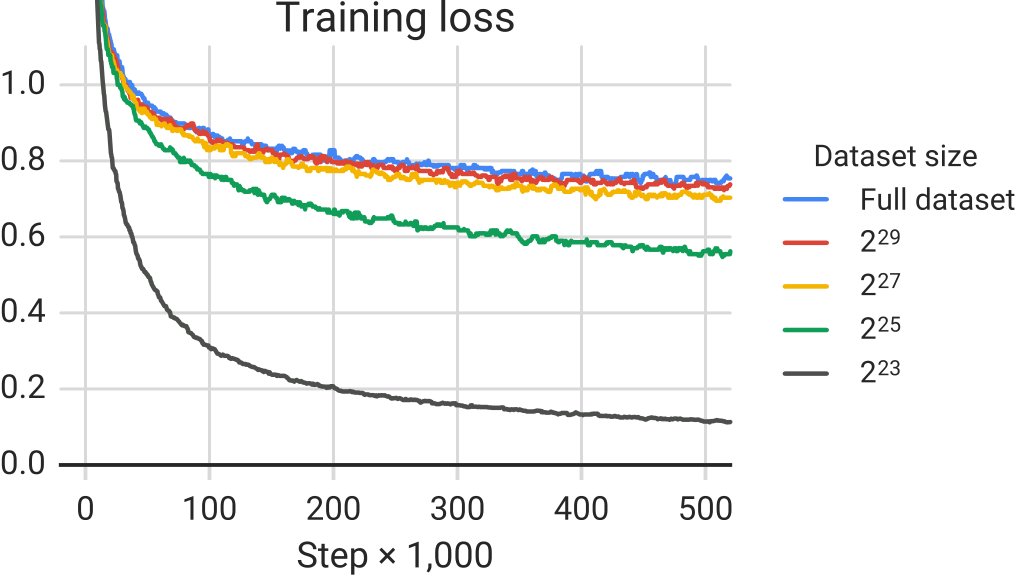
Figure 6: Pre-training loss for our original C4 data set as well as artificially truncated versions. The sizes listed refer to the number of tokens in each data set. The four sizes considered correspond to repeating the data set between and times over the course of pre-training. Using a smaller data set size results in smaller training loss values, which may suggest some memorization of the unlabeled data set.
图6:我们原先的C4数据集以及人工截断版本的培训前损失。 列出的大小是指每个数据集中的符数. 所考虑的四种尺寸对应于在训练前期间重复至之间的数据集. 使用较小的数据集大小导致培训损失值较小,这可能意味着对未贴标签的数据集进行一定的记忆.
3.5 Training Strategy
3.5 训练策略
So far we have considered the setting where all parameters of a model are pre-trained on an unsupervised task before being fine-tuned on individual supervised tasks. While this approach is straightforward, various alternative methods for training the model on downstream/supervised tasks have been proposed. In this section, we compare different schemes for fine-tuning the model in addition to the approach of training the model simultaneously on multiple tasks.
迄今为止,我们考虑了一种模式的所有参数在对个别受监督的任务进行微调之前预先就一项不受监督的任务进行培训的情况。 虽然这种做法是直截了当的,但已经提出了各种替代方法,用于培训下游/监督任务的模式。 在本节中,我们比较了对模型进行微调的不同方案,以及同时对模型进行多重任务培训的方法。
3.5.1 Fine-tuning Methods
It has been argued that fine-tuning all of the model’s parameters can lead to suboptimal results, particularly on low-resource tasks (Peters et al. 2019). Early results on transfer learning for text classification tasks advocated fine-tuning only the parameters of a small classifier that was fed sentence embeddings produced by a fixed pre-trained model (Subramanian et al. 2018; Kiros et al. 2015; Logeswaran and Lee 2018; Hill et al. 2016; Conneau et al. 2017). This approach is less applicable to our encoder-decoder model because the entire decoder must be trained to output the target sequences for a given task. Instead, we focus on two alternative fine-tuning approaches that update only a subset of the parameters of our encoder-decoder model.
3.5.1 微调方法
有人认为,对模型的所有参数进行微调可导致不理想的结果,特别是在低资源任务方面(Peters等人,2019年)。 文本分类任务转移学习的早期结果主张绷紧一个小分类器的参数,该分类器是由固定的预训模型所生成的输入句子嵌入(Subramanian等人,2018年;Kiros等人,2015年;Logeswaran和Lee 2018年;Hill等人,2016年;Conneau等人,2017年). 这种方法不太适用于我们的编码器-解码器模型,因为整个解码器必须经过训练才能输出特定任务的目标序列. 相反,我们侧重于两种备选的微调方法,它们只更新我们编码器-解码器模型的一个参数子集。
The first, “adapter layers” (Houlsby et al. 2019; Bapna et al. 2019), is motivated by the goal of keeping most of the original model fixed while fine-tuning. Adapter layers are additional dense-ReLU-dense blocks that are added after each of the preexisting feed-forward networks in each block of the Transformer. These new feed-forward networks are designed so that their output dimensionality matches their input. This allows them to be inserted into the network with no additional changes to the structure or parameters. When fine-tuning, only the adapter layer and layer normalization parameters are updated. The main hyperparameter of this approach is the inner dimensionality of the feed-forward network, which changes the number of new parameters added to the model. We experiment with various values for .
第一层是“适应层”(Houlsby等人,2019年;Bapna等人,2019年),其动机是保持大多数原始模型的固定和微调。 适配器层是额外的稠密-ReLU-dense区块,这些区块是在Transformer每个区块中每个原有的向导网络之后添加的. 这些新的信息传输网络的设计是为了使其输出维度与其输入值相匹配。 这使得它们可以被插入到网络中,而不对结构或参数进行额外的修改. 在微调时,只更新适配器层和层常态参数. 这种方法的主要超参数是向导网络的内维度,它改变了模型中新增参数的数量. 我们对的各种数值进行了试验。
The second alternative fine-tuning method we consider is “gradual unfreezing” (Howard and Ruder 2018). In gradual unfreezing, more and more of the model’s parameters are fine-tuned over time. Gradual unfreezing was originally applied to a language model architecture consisting of a single stack of layers. In this setting, at the start of fine-tuning only the parameters of the final layer are updated, then after training for a certain number of updates the parameters of the second-to-last layer are also included, and so on until the entire network’s parameters are being fine-tuned. To adapt this approach to our encoder-decoder model, we gradually unfreeze layers in the encoder and decoder in parallel, starting from the top in both cases. Since the parameters of our input embedding matrix and output classification matrix are shared, we update them throughout fine-tuning. Recall that our baseline model consists of layers each in the encoder and decoder and is fine-tuned for steps. As such, we subdivide the fine-tuning process into episodes of steps each and train from layers to in the th episode. We note that Howard and Ruder 2018 suggested fine-tuning an additional layer after each epoch of training. However, since our supervised data sets vary so much in size and since some of our downstream tasks are actually mixtures of many tasks (GLUE and SuperGLUE), we instead adopt the simpler strategy of fine-tuning an additional layer after every steps.
我们认为,第二个备选微调方法是“逐步解冻”(Howard和Ruder 2018)。 在逐渐解冻的过程中,越来越多的模型参数随着时间推移进行了微调. 渐渐解冻最初应用于由单叠层组成的语言模型架构. 在此设定中,在微调开始时,只更新最后一层的参数,然后在经过一定数量的更新培训后,将第二层至最后一层 319的汪精卫的参数也包括在内,直至整个网络的参数被微调. 为了使这种方法适应我们的编码器-解码器模型,我们逐渐解冻编码器中的层层,并平行解码器,两种情况下从顶部开始. 由于我们输入嵌入矩阵和产出分类矩阵的参数是共享的,我们在整个微调过程中对其进行更新。 回顾我们的基线模型由编码器和解码器中的层各组成,并对步骤进行了微调. 因此,我们将微调过程细分为集,每集为步,并在集中从第至层列车. 我们注意到,Howard和Ruder 2018建议在每个培训时期之后再调整一层。 然而,由于我们所监管的数据集在大小上差异很大,并且由于我们的一些下游任务实际上是许多任务的混合体(GLUE和SuperGLUE),因此我们采取了在每步骤后细化一层的简单战略.
A comparison of the performance of these fine-tuning approaches is shown in Table 10. For adapter layers, we report the performance using an inner dimensionality of , , , . Pursuant with past results (Houlsby et al. 2019; Bapna et al. 2019) we find that lower-resource tasks like SQuAD work well with a small value of whereas higher resource tasks require a large dimensionality to achieve reasonable performance. This suggests that adapter layers could be a promising technique for fine-tuning on fewer parameters as long as the dimensionality is scaled appropriately to the task size. Note that in our case we treat GLUE and SuperGLUE each as a single “task” by concatenating their constituent data sets, so although they comprise some low-resource data sets the combined data set is large enough that it necessitates a large value of . We found that gradual unfreezing caused a minor degradation in performance across all tasks, though it did provide some speedup during fine-tuning. Better results may be attainable by more carefully tuning the unfreezing schedule.
表10比较了这些微调方法的业绩。 对于适配层,我们使用的内维度,,,的内维度报告性能. 根据以往的结果(Houlsby等人,2019年;Bapna等人,2019年),我们发现,像SQuAD这样的低资源任务效果良好,价值小于,而更高的资源任务则需要很大的维度才能实现合理的性能. 这表明,只要能适当按照任务规模调整维度,适配器层就可能成为在较少参数上微调的一种有希望的技术。 请注意,就我们的情况而言,我们把GLUE和SuperGLUE各自作为一个单一的“任务”来对待,办法是将其组成数据集压缩,因此,尽管它们包括一些低资源数据集,但综合数据集足够大,因此需要大量的值。 我们发现,逐渐解冻导致所有任务的业绩略有下降,尽管在微调时确实提供了一些速度。 通过更仔细地调整解冻时间表,可以取得更好的结果。
| Fine-tuning method | GLUE | CNNDM | SQuAD | SGLUE | EnDe | EnFr | EnRo |
|---|---|---|---|---|---|---|---|
| All parameters | |||||||
| Adapter layers, | |||||||
| Adapter layers, | |||||||
| Adapter layers, | |||||||
| Adapter layers, | |||||||
| Gradual unfreezing |
Table 10: Comparison of different alternative fine-tuning methods that only update a subset of the model’s parameters. For adapter layers, refers to the inner dimensionality of the adapters.
| 微调方法 | 格吕 | CNNDM( CNNDM ) : 美国主题 美国主题 美国主题 美国主题 美国主题 美国主题 美国主题 | SQAD 状态 | 英格兰 | 定义 | 定义Fr | 恩罗 |
|---|---|---|---|---|---|---|---|
| 第二十届 所有参数 | |||||||
| 适配层, | |||||||
| 适配层, | |||||||
| 适配层, | |||||||
| 适配层, | |||||||
| 逐渐解冻 |
表10 别担心,对不同的备选微调方法进行比较,这些方法只更新模型参数的一个子集。 对于适配器层,指的是适配器的内在维度.
3.5.2 Multi-task Learning
So far, we have been pre-training our model on a single unsupervised learning task before fine-tuning it individually on each downstream task. An alternative approach, called “multi-task learning” (Ruder 2017; Caruana 1997), is to train the model on multiple tasks at a time. This approach typically has the goal of training a single model that can simultaneously perform many tasks at once, i.e. the model and most of its parameters are shared across all tasks. We relax this goal somewhat and instead investigate methods for training on multiple tasks at once in order to eventually produce separate parameter settings that perform well on each individual task. For example, we might train a single model on many tasks, but when reporting performance we are allowed to select a different checkpoint for each task. This loosens the multi-task learning framework and puts it on more even footing compared to the pre-train-then-fine-tune approach we have considered so far. We also note that in our unified text-to-text framework, “multi-task learning” simply corresponds to mixing data sets together. It follows that we can still train on unlabeled data when using multi-task learning by treating the unsupervised task as one of the tasks being mixed together. In contrast, most applications of multi-task learning to NLP add task-specific classification networks or use different loss functions for each task (Liu et al. 2019b).
3.5.2 多任务学习
迄今为止,我们一直在就一项单一的无监督的学习任务对我们的模式进行预先培训,然后对每项下游任务进行个别的调整。 另一种称为“多任务学习”的办法(Ruder 2017;Caruana 1997)是一次对模式进行多任务培训。 这种方法通常的目标是培训一个能够同时完成许多任务的单一模式,即该模式及其大多数参数在所有任务中共享。 我们稍稍放松这一目标,而是立即调查多种任务的培训方法,以便最终产生单独的参数设置,很好地完成每项任务。 例如,我们可以对许多任务进行单一模式的培训,但在报告业绩时,我们可以为每项任务选择不同的检查站。 这缇松了多任务学习框架,使之比迄今为止我们考虑的训练前和精准 28. 更平衡。 我们还注意到,在我们统一的文本对文本框架中,“多任务学习”仅仅相当于将数据集混合在一起。 因此,在使用多任务学习时,我们仍可以对未加标签的数据进行培训,将未受监督的任务作为混合的任务之一。 对比之下 你的多任务学习在NLP中的大多数应用都加入了任务特定分类网络,或者对每项任务使用不同的损失功能(Liu等人,2019年b).
As pointed out by Arivazhagan et al. 2019, an extremely important factor in multi-task learning is how much data from each task the model should be trained on. Our goal is to not under- or over-train the model—that is, we want the model to see enough data from a given task that it can perform the task well, but not to see so much data that it memorizes the training set. How exactly to set the proportion of data coming from each task can depend on various factors including data set sizes, the “difficulty” of learning the task (i.e. how much data the model must see before being able to perform the task effectively), regularization, etc. An additional issue is the potential for “task interference” or “negative transfer”, where achieving good performance on one task can hinder performance on another. Given these concerns, we begin by exploring various strategies for setting the proportion of data coming from each task. A similar exploration was performed by Wang et al. 2019a.
正如Arivazhagan等人2019年所指出的,多任务学习中一个极为重要的因素,就是每个任务中应培训多少数据。 我们的目标是不低估或过度训练这一模式——即我们希望该模式能够从特定的任务中看到足够的数据,以便它能够很好地完成任务,但不能看到如此多的数据,以至于它能记住训练集。 如何准确确定每项任务体现了的数据比例取决于各种因素,包括数据集大小、学习任务的“困难”(即模型在能够有效完成任务之前必须看到多少数据)、正规化等。 另一个问题是“任务干预”或“负转移”的可能性,因为一项任务取得良好业绩会妨碍另一项任务的执行。 鉴于这些关切,我们首先探讨各种战略,以确定每项任务的数据比例。 王等2019a进行了类似的探索.
A major factor in how quickly a model will overfit to a given task is the task’s data set size. As such, a natural way to set the mixing proportions is to sample in proportion to the size of each task’s data set. This is equivalent to concatenating the data sets for all tasks and randomly sampling examples from the combined data set. Note, however, that we are including our unsupervised denoising task, which uses a data set that is orders of magnitude larger than every other task’s. It follows that if we simply sample in proportion to each data set’s size, the vast majority of the data the model sees will be unlabeled, and it will undertrain on all of the supervised tasks. Even without the unsupervised task, some tasks (e.g. WMT English to French) are so large that they would similarly crowd out most of the batches. To get around this issue, we set an artificial “limit” on the data set sizes before computing the proportions. Specifically, if the number of examples in each of our task’s data sets is then we set probability of sampling an example from the th task during training to where is the artificial data set size limit.
一个模型对某项任务的过度适应速度的一个主要因素是任务的数据集大小。 因此,确定混合比例的自然方法是按照每个任务数据集的规模进行抽样。 这相当于整理所有任务的数据集和从合并数据集中随机取样的例子. 然而,请注意,我们正在列入我们未经监督的取消提名的任务,它使用一个比其他每一项任务都大的数量级的数据集。 因此,如果我们简单地按照每个数据集的大小进行抽样,模型所看到的绝大多数数据将得不到标签,它将对所有监督任务进行不足。 即使没有不受监督的任务,一些任务(例如WMT英语到法语)也很大,同样会挤出大部分批次. 为了绕过这一问题,我们在计算比例之前对数据集大小设定了人为的“限制”。 具体地说,如果我们的任务数据集中的每一组例数是,那么我们就设定了在训练期间从第2次任务中取样一个例的概率到,其中是人工数据集大小限制.
An alternative way of mitigating the huge disparity between data set sizes is to adjust the ‘‘temperature’’ of the mixing rates. This approach was used by multilingual BERT to ensure that the model was sufficiently trained on low-resource languages.[^14] To implement temperature scaling with temperature , we raise each task’s mixing rate to the power of \nicefrac{{1}}{{T}} and renormalize the rates so that they sum to 1. When , this approach is equivalent to examples-proportional mixing and as increases the proportions become closer to equal mixing. We retain the data set size limit (applied to obtain before temperature scaling) but set it to a large value of . We use a large value of because increasing the temperature will decrease the mixing rate of the largest data sets.
减轻数据集大小之间巨大差距的另一种办法是调整混合率的温度。 多种语文的BERT采用了这种方法,以确保该模式得到充分的低资源语言培训。 为了与温度进行温度缩放,我们将每个任务的混合速率提高到\nicefrac{{1}}{{T}}的功率,并重新规范速率,使其合为 1. 当时,这个方法相当于例-比例混合,随着的提高比例越来越接近于等位混合. 我们保留了数据集的尺寸限制(在温度缩放前用于获得),但将其设定为大值为. 我们使用大量的值,因为提高温度会降低最大数据集的混合率.
In this case, we sample examples from each task with equal probability. Specifically, each example in each batch is sampled uniformly at random from one of the data sets we train on. This is most likely a suboptimal strategy, as the model will overfit quickly on low-resource tasks and underfit on high-resource tasks. We mainly include it as a point of reference of what might go wrong when the proportions are set suboptimally.
在这种情况下,我们以同样的可能性对每项任务的实例进行抽样。 具体来说,每个批次中的每一例都从我们训练的数据集中随机抽取统一样本. 这很可能是一个不尽人意的战略,因为模型将很快适应于低资源任务和高资源任务。 我们主要把它作为衡量在比例不理想的情况下可能出现错误的参照点。
To compare these mixing strategies on equal footing with our baseline pre-train-then-fine-tune results, we train multi-task models for the same total number of steps: . The results are shown in Table 11.
为了在平等的基础上将这些混合战略与我们的基线培训前结果进行比较,我们为相同的步骤总数培训多种任务模式:。 结果见表11。
In general, we find that multi-task training underperforms pre-training followed by fine-tuning on most tasks. The “equal” mixing strategy in particular results in dramatically degraded performance, which may be because the low-resource tasks have overfit, the high-resource tasks have not seen enough data, or the model has not seen enough unlabeled data to learn general-purpose language capabilities. For examples-proportional mixing, we find that for most tasks there is a “sweet spot” for where the model obtains the best performance, and larger or smaller values of tend to result in worse performance. The exception (for the range of values we considered) was WMT English to French translation, which is such a high-resource task that it always benefits from a higher mixing proportion. Finally, we note that temperature-scaled mixing also provides a means of obtaining reasonable performance from most tasks, with performing the best in most cases. The finding that a multi-task model is outperformed by separate models trained on each individual task has previously been observed e.g. by Arivazhagan et al. 2019 and McCann et al. 2018, though it has been shown that the multi-task setup can confer benefits across very similar tasks Liu et al. 2019b; Ratner et al. 2018. In the following section, we explore ways to close the gap between multi-task training and the pre-train-then-fine-tune approach.
总的来说,我们发现,多任务培训在培训前表现不佳,然后对大多数任务进行微调。 “平等”混合战略尤其导致业绩急剧下降,这可能是因为低资源任务过于适应,高资源任务没有看到足够的数据,或者模型没有看到足够的无标签数据来学习通用语言能力。 关于实例-比例混合,我们发现,对于大多数任务来说,在中有一个“甜点”,模型在其中获得最佳性能,而的较大或较小值往往导致性能差。 特例(我们所考虑的值范围)是WMT英文译为法文译文,这是一项高资源任务,总能从较高的混合比例中受益. 最后,我们注意到,温度尺度的混合还提供了从大多数任务中获得合理性能的手段,在多数情况下,表现最好。 Arivazhagan等人(2019年)和McCann等人(2018年)曾观察到过这样一个结论,即一项多任务模式的绩效超过了就每项单独任务培训的单独模式,尽管已经表明,多任务设置可以给刘等人(2019年的条款);Ratner等人(2018年条款)。 在下一节中,我们探索如何弥合多任务培训与前期培训法之间的空白。
| Mixing strategy | GLUE | CNNDM | SQuAD | SGLUE | EnDe | EnFr | EnRo |
|---|---|---|---|---|---|---|---|
| Baseline (pre-train/fine-tune) | |||||||
| Equal | |||||||
| Examples-proportional, | |||||||
| Examples-proportional, | |||||||
| Examples-proportional, | |||||||
| Examples-proportional, | |||||||
| Examples-proportional, | |||||||
| Examples-proportional, | |||||||
| Temperature-scaled, | |||||||
| Temperature-scaled, | |||||||
| Temperature-scaled, |
Table 11: Comparison of multi-task training using different mixing strategies. Examples-proportional mixing refers to sampling examples from each data set according to the total size of each data set, with an artificial limit () on the maximum data set size. Temperature-scaled mixing re-scales the sampling rates by a temperature . For temperature-scaled mixing, we use an artificial data set size limit of .
| 混合战略 | 格吕 | CNNDM( CNNDM ) : 美国主题 美国主题 美国主题 美国主题 美国主题 美国主题 美国主题 | SQAD 状态 | 英格兰 | 定义 | 定义Fr | 恩罗 |
|---|---|---|---|---|---|---|---|
| 基准(培训前/调整) | |||||||
| 平等 | |||||||
| 实例比例, | |||||||
| 实例比例, | |||||||
| 实例比例, | |||||||
| 实例比例, | |||||||
| 实例比例, | |||||||
| 实例比例, | |||||||
| 温度尺度, | |||||||
| 温度尺度, | |||||||
| 温度尺度, |
表11:采用不同混合策略的多任务培训比较. 示例-比例混合是指根据每个数据集的总大小从每个数据集中采集的样本实例,在最大数据集大小上有一个人为的极限(). 温度尺度混合以温度重新测定采样率。 对于温度尺度的混合,我们使用的人工数据集尺寸限制.
3.5.3 Combining Multi-Task Learning with Fine-Tuning
Recall that we are studying a relaxed version of multi-task learning where we train a single model on a mixture of tasks but are allowed to evaluate performance using different parameter settings (checkpoints) for the model. We can extend this approach by considering the case where the model is pre-trained on all tasks at once but is then fine-tuned on the individual supervised tasks. This is the method used by the “MT-DNN” (Liu et al. 2015; Liu et al. 2019b), which achieved state-of-the-art performance on GLUE and other benchmarks when it was introduced. We consider three variants of this approach: In the first, we simply pre-train the model on an examples-proportional mixture with an artificial data set size limit of before fine-tuning it on each individual downstream task. This helps us measure whether including the supervised tasks alongside the unsupervised objective during pre-training gives the model some beneficial early exposure to the downstream tasks. We might also hope that mixing in many sources of supervision could help the pre-trained model obtain a more general set of “skills” (loosely speaking) before it is adapted to an individual task. To measure this directly, we consider a second variant where we pre-train the model on the same examples-proportional mixture (with ) except that we omit one of the downstream tasks from this pre-training mixture. Then, we fine-tune the model on the task that was left out during pre-training. We repeat this for each of the downstream tasks we consider. We call this approach “leave-one-out” multi-task training. This simulates the real-world setting where a pre-trained model is fine-tuned on a task it had not seen during pre-training. Note that multi-task pre-training provides a diverse mixture of supervised tasks. Since other fields (e.g. computer vision (Oquab et al. 2014; Jia et al. 2014; Huh et al. 2016; Yosinski et al. 2014)) use a supervised data set for pre-training, we were interested to see whether omitting the unsupervised task from the multi-task pre-training mixture still produced good results. For our third variant we therefore pre-train on an examples-proportional mixture of all of the supervised tasks we consider with . In all of these variants, we follow our standard procedure of pre-training for steps before fine-tuning for steps.
3.5.3 将多任务学习与精细学习相结合
记得我们正在研究一个放松的多任务学习版本,在这个版本中,我们在任务组合上训练一个单一的模型,但允许使用不同的参数设置(检查点)来评价模型的性能. 我们可以通过考虑以下情况来扩大这一方法:该模式立即对所有任务进行预先培训,然后对个别监督任务进行微调。 这是“MT-DNN”(Liu等人,2015年;Liu等人,2019年b)采用的方法,在采用GLUE和其他基准时取得了最新业绩。 我们认为这种办法有三个变式: 在第一部分中,我们只是先对模型进行关于实例-比例混合物的预演,人工数据集尺寸限制为,然后对每个下游任务进行微调。 这有助于我们衡量在培训前将受监督的任务与未受监督的目标一起纳入,是否使该模式在早期就对下游任务有所帮助。 我们还希望,在许多监督来源的混合有助于预先培训的模式在适应个别任务之前获得一套更普遍的“技能”(略微地说)。 为了直接衡量这一点,我们考虑了第二个变体,即我们用同样的实例-比例混合物(与)对模型进行预先培训,只是我们从这种预培训混合物中省略了一个下游任务。 然后,我们微调了模式 在训练前被忽略的任务。 我们在考虑的每一项下游任务中都重复这一点。 我们称这种做法为“一劳永逸”的多任务培训。 这模拟了现实世界的设置,即预先训练的模型在训练前所未见的任务上得到微调。 请注意,多任务前培训提供了多种监督任务的组合。 由于其他领域(如计算机视觉(Oquab等人,2014年;Jia等人,2014年;Huh等人,2016年;Yosinski等人,2014年)使用受监督的数据集进行预训,我们很想知道在多任务预训混合物中省略未监督的任务是否仍然产生良好效果. 因此,对于我们的第三个变式,我们先就我们与一起审议的所有受监督任务的样例和比例混合进行预训。 在所有这些变式中,我们遵循我们的步骤预训标准程序,然后对步骤进行微调。
| Training strategy | GLUE | CNNDM | SQuAD | SGLUE | EnDe | EnFr | EnRo |
|---|---|---|---|---|---|---|---|
| Unsupervised pre-training + fine-tuning | |||||||
| Multi-task training | |||||||
| Multi-task pre-training + fine-tuning | |||||||
| Leave-one-out multi-task training | |||||||
| Supervised multi-task pre-training |
Table 12: Comparison of unsupervised pre-training, multi-task learning, and various forms of multi-task pre-training.
| 培训战略 | 格卢 | CNNDM( CNNDM ) : 美国主题 美国主题 美国主题 美国主题 美国主题 美国主题 美国主题 | SQAD 状态 | 英格兰 | 定义 | 定义Fr | 恩罗 |
|---|---|---|---|---|---|---|---|
| 未经监督的预训+微调 | |||||||
| 多任务培训 | |||||||
| 多任务前培训+微调 | |||||||
| 多任务培训 | |||||||
| 监督的多任务前培训 |
表12:无监督的预训,多任务学习以及多种形式多任务预训的比较.
We compare the results of these approaches in Table 12. For comparison, we also include results for our baseline (pre-train then fine-tune) and for standard multi-task learning (without fine-tuning) on an examples-proportional mixture with . We find that fine-tuning after multi-task pre-training results in comparable performance to our baseline. This suggests that using fine-tuning after multi-task learning can help mitigate some of the trade-offs between different mixing rates described in Section 3.5.2. Interestingly, the performance of “leave-one-out” training was only slightly worse, suggesting that a model that was trained on a variety of tasks can still adapt to new tasks (i.e. multi-task pre-training might not result in a dramatic task interference). Finally, supervised multi-task pre-training performed significantly worse in every case except for the translation tasks. This could suggest that the translation tasks benefit less from (English) pre-training, whereas unsupervised pre-training is an important factor in the other tasks.
我们在表12中比较了这些方法的结果。 为了进行比较,我们还列入了基线(培训前再作微调)以及标准多任务学习(不作微调)与进行实例-比例混合的结果。 我们认为,经过多任务前培训后的微调,结果与我们的基线具有可比性。 这表明,在多任务学习后进行微调有助于减轻第3.5.2节所述不同混合率之间的一些权衡。 有趣的是,“一劳永逸”培训的成绩只是略微差一些,这表明接受各种任务培训的模式仍然能够适应新的任务(即多任务前培训可能不会造成戏剧性的任务干扰)。 最后,除翻译工作外,在监督下进行的多任务前培训在所有情况下都表现得更差。 这可能表明翻译任务从(英语)预训中受益较少,而无监督的预训则是其他任务的一个重要因素.
3.6 Scaling
3.6 规模扩展
The “bitter lesson” of machine learning research argues that general methods that can leverage additional computation ultimately win out against methods that rely on human expertise (Sutton 2019; Hestness et al. 2017; Shazeer et al. 2017; Jozefowicz et al. 2016; Mahajan et al. 2018; Shazeer et al. 2018; Shazeer et al. 2017; Huang et al. 2018b; Keskar et al. 2019a). Recent results suggest that this may hold true for transfer learning in NLP (Liu et al. 2019c; Radford et al. 2019; Yang et al. 2019; Lan et al. 2019), i.e. it has repeatedly been shown that scaling up produces improved performance compared to more carefully-engineered methods. However, there are a variety of possible ways to scale, including using a bigger model, training the model for more steps, and ensembling. In this section, we compare these different approaches by addressing the following premise: “You were just given more compute. How should you use it?”
机器学习研究的"痛苦教训"认为,能够利用额外计算最终战胜依赖人类专业知识的方法的一般方法(Sutton 2019;Hestness等人 2017;Shazeer等人 2017;Jozefowicz等人 2016;Mahajan等人 2018;Shazeer等人 2018;Shazeer等人 2017;Huang等人 2018b;Keskar等人 2019a). 近期的结果表明,在NLP中(Liu等人,2019年c;Radford等人,2019年;Yang等人,2019年;Lan等人,2019年),转学学习中可能存在这种情况,也就是说,已经反复表明,与更仔细地设计的方法相比,扩大规模可以提高绩效。 然而,有多种可能的尺度化方法,包括使用更大的模型,对模型进行更多步骤的培训,以及综艺. 在本节中,我们比较了这些不同的做法,其前提如下:“刚刚给了你更多的计算。 应如何使用?”
We start with our baseline model, which has parameters and is pre-trained and fine-tuned for and steps respectively. The encoder and decoder are both sized similarly to “BERTBASE”. To experiment with increased model size, we follow the guidelines of “BERTLARGE” Devlin et al. 2018 and use , , and -head attention mechanisms. We then generate two variants with and layers each in the encoder and decoder, producing models with and as many parameters as our original model. These two variants also have a roughly and the computational cost. Using our baseline and these two larger models, we consider three ways of using as much computation: Training for as many steps, training for as many steps with the bigger model, and training the bigger model for the “baseline” number of training steps. When we increase the training steps, we scale both the pre-train and fine-tune steps for simplicity. Note that when increasing the number of pre-training steps, we are effectively including more pre-training data as C4 is so large that we do not complete one pass over the data even when training for steps.
我们从基线模型开始,该模型有参数,并对和步骤分别进行了预先培训和微调。 编码器和解码器的尺寸都类似于“BERTBASE”。 为了试验扩大模型规模,我们遵循“BERTLARGE”Devlin等人2018年准则,并使用、、和-头部注意机制。 然后,我们在编码器和解码器中分别生成两个带有和层的变体,生成具有和的参数与我们最初的模型一样多的模型. 这两个变体还有大约和的计算成本. 利用我们的基线和这两个更大的模型,我们考虑了使用的三种方法,如计算: 对的培训是许多步骤,对的培训是许多步骤,采用大模式,对大模式的培训是“基线”培训步骤的数目。 当我们增加训练步骤时,我们既扩大训练前步骤,也扩大精细调整步骤,以便做到简单。 请注意,在增加培训前步骤的数量时,我们有效地纳入了更多的培训前数据,因为C4如此之大,即使为步骤进行培训,我们也无法完成一个数据传递。
An alternative way for the model to see as much data is to increase the batch size by a factor of . This can potentially result in faster training due to more efficient parallelization. However, training with a larger batch size can yield a different outcome than training for as many steps (Shallue et al. 2018). We include an additional experiment where we train our baseline model with a larger batch size to compare these two cases.
模型将看成大量数据的另一种方法是将批量大小增加的系数. 由于更有效率的平行化,这有可能加快培训。 然而,使用大批量规模的培训可以产生与培训不同的结果,因为有许多步骤(Shallue等人,2018年)。 我们增加了一个试验,即我们用更大的批量规模来培训我们的基线模型,以比较这两个案例。
It is common practice on many of the benchmarks we consider to eke out additional performance by training and evaluating using an ensemble of models. This provides an orthogonal way of using additional computation. To compare other scaling methods to ensembling, we also measure the performance of an ensemble of separately pre-trained and fine-tuned models. We average the logits across the ensemble before feeding them into the output nonlinearity to obtain an aggregate prediction. Instead of pre-training separate models, a cheaper alternative is to take a single pre-trained model and produce separate fine-tuned versions. While this does not use our entire computational budget, we also include this method to see if it produces competitive performance to the other scaling methods.
在我们考虑的许多基准中,通常的做法是通过培训和使用一套模型来评估额外的业绩。 这提供了使用额外计算的一种正统方法。 为了将其他的缩放方法与综艺比较,我们还测量了一套由分开的预训和微调模型的性能. 在输入输出的非线性之前,我们平均对数值。 与预训分离型号不同,更便宜的替代品是采用单一预训型号,生产分离的微调版本. 虽然这并没有使用我们的整个计算预算,但我们也包含了这一方法,以查看它是否产生与其他缩放方法的竞争性性能.
| Scaling strategy | GLUE | CNNDM | SQuAD | SGLUE | EnDe | EnFr | EnRo |
|---|---|---|---|---|---|---|---|
| Baseline | |||||||
| size, training steps | |||||||
| size, batch size | |||||||
| size, training steps | |||||||
| size, training steps | |||||||
| ensembled | |||||||
| ensembled, fine-tune only |
Table 13: Comparison of different methods of scaling up our baseline model. All methods except ensembling fine-tuned models use the computation as the baseline. “Size” refers to the number of parameters in the model and “training time” refers to the number of steps used for both pre-training and fine-tuning.
| 扩大战略 | 格吕 | CNNDM( CNNDM ) : 美国主题 美国主题 美国主题 美国主题 美国主题 美国主题 美国主题 | SQAD 状态 | 英格兰 | 定义 | 定义Fr | 恩罗 |
|---|---|---|---|---|---|---|---|
| 基线 | |||||||
| 规模,培训步骤 | |||||||
| 大小,批量大小 | |||||||
| 规模,培训步骤 | |||||||
| 规模,培训步骤 | |||||||
| 组合 | |||||||
| 组合,仅微调 |
表13:扩大基线模型的不同方法比较。 除综艺微调模型外,所有方法都使用作为基准。 “规模”是指模型中的参数数,“培训时间”是指用于培训前和微调的步骤数。
The performance achieved after applying these various scaling methods is shown in Table 13. Unsurprisingly, increasing the training time and/or model size consistently improves the baseline. There was no clear winner between training for as many steps or using a larger batch size, though both were beneficial. In general, increasing the model size resulted in an additional bump in performance compared to solely increasing the training time or batch size. We did not observe a large difference between training a bigger model for as long and training a bigger model on any of the tasks we studied. This suggests that increasing the training time and increasing the model size can be complementary means of improving performance. Our results also suggest that ensembling provides an orthogonal and effective means of improving performance through scale. In some tasks (CNN/DM, WMT English to German, and WMT English to Romanian), ensembling completely separately trained models significantly outperformed every other scaling approach. Ensembling models that were pre-trained together but fine-tuned separately also gave a substantial performance increase over the baseline, which suggests a cheaper means of improving performance. The only exception was SuperGLUE, where neither ensembling approach significantly improved over the baseline.
采用这些各种缩放方法后取得的业绩见表13。 不足为奇的是,增加培训时间和(或)模型规模不断改善基线。 在的训练与许多步骤之间,或者使用更大的批量规模之间,并没有明确的获胜者,尽管两者都是有益的. 一般说来,由于模型规模的扩大,与仅仅增加培训时间或批量规模相比,性能也出现了新的颠峰。 我们没有观察到在为培训一个更大的模型与就我们所研究的任何任务培训一个更大的模型之间有很大的区别。 这表明,增加培训时间和增加模式规模可以成为改进业绩的补充手段。 我们的成果还表明,综艺为通过规模提高业绩提供了一种正统和有效的手段。 在一些任务中(CNN/DM,WMT英语对德语,WMT英语对罗马尼亚语),综艺完全单独训练的模型显著超过所有其他的缩放方法. 结合预先一起训练但分别加以微调的模型,也使业绩大大高于基线,这表明改进业绩的较廉价手段。 唯一的例外是SuperGLUE,其中综艺方法都比基线大有改进。
We note that different scaling methods have different trade-offs that are separate from their performance. For example, using a larger model can make downstream fine-tuning and inference more expensive. In contrast, the cost of pre-training a small model for longer is effectively amortized if it is applied to many downstream tasks. Separately, we note that ensembling separate models has a similar cost to using a model that has an higher computational cost. As a result, some consideration for the eventual use of the model is important when choosing between scaling methods.
我们注意到,不同的衡量方法有不同的取舍,这些取舍与其业绩不同。 例如,使用更大的模型可以使下游的微调和推论更加昂贵. 与此相反,如果将小型模型应用于许多下游任务,则该模型较长时间的预训费用将有效摊销。 另外,我们注意到,综艺独立模型的成本与使用计算成本较高的模型的成本类似。 因此,在选择衡量方法时,考虑最终使用该模型很重要。
3.7 Putting It All Together
3.7 综合起来
We now leverage the insights from our systematic study to determine how far we can push performance on popular NLP benchmarks. We are also interested in exploring the current limits of transfer learning for NLP by training larger models on large amounts of data. We start with our baseline training approach and make the following changes:
我们现在利用我们系统研究的洞察力,确定我们能够在多大程度上推动在受欢迎的NLP基准方面的业绩。 我们还有兴趣探索目前为NLP进行转移学习的限度,办法是在大量数据方面培训更大的模型。 我们首先采取基线培训办法,并作出以下修改:
We swap out the i.i.d. denoising objective in our baseline for the span-corruption objective described in Section 3.3.4, which was loosely inspired by SpanBERT (Joshi et al. 2019). Specifically, we use a mean span length of and corrupt of the original sequence. We found that this objective produced marginally better performance (Table 7) while being slightly more computationally efficient due to shorter target sequence lengths.
我们将第3.3.4节所述跨度腐败目标的基线中代言目标交换出去,后者受到SpanBERT(Joshi等人,2019年)松散的启发。 具体来说,我们使用的是的中间跨度,以及原序列中腐败的. 我们发现,由于目标序列长度较短,这一目标的性能略好一些(表7)。
Our baseline model uses a relatively small amount of pre-training ( as much as BERT (Devlin et al. 2018), as much as XLNet (Yang et al. 2019), as much as RoBERTa (Liu et al. 2019c), etc.). Fortunately, C4 is big enough that we can train for substantially longer without repeating data (which can be detrimental, as shown in Section 3.4.2). We found in Section 3.6 that additional pre-training can indeed be helpful, and that both increasing the batch size and increasing the number of training steps can confer this benefit. We therefore pre-train our models for million steps on a batch size of sequences of length , corresponding to a total of about trillion pre-training tokens (about as many as our baseline). In Section 3.4.1, we showed that pre-training on the RealNews-like, WebText-like, and Wikipedia + TBC data sets outperformed pre-training on C4 on a few downstream tasks. However, these data set variants are sufficiently small that they would be repeated hundreds of times over the course of pre-training on trillion tokens. Since we showed in Section 3.4.2 that this repetition could be harmful, we opted instead to continue using the C4 data set.
我国基准模式使用量相对较小的预训(与BERT(Devlin等人,2018年),与XLNet(Yang等人,2019年),与RoBERTa(Liu等人,2019年c)等相当). 幸运的是,C4足够大,我们可以在不重复数据的情况下训练更长的时间(如第3.4.2节所示,这可能有害)。 我们在第3.6节中发现,额外预训确实会有所帮助,增加批量规模和增加培训步骤的数量都能够带来这种好处。 因此,我们按长的批量大小对百万步的模型进行预训,相当于大约万亿兆的预训符号(大约与我们的基线一样多)。 在3.4.1节中,我们显示关于RealNews类,WebText类,以及维基百科+TBC数据的预训,在几个下游任务上,C4的预训都完成了. 然而,这些数据集变体足够小,在万亿令牌的预训过程中会重复数百次. 由于我们在第3.4.2节中表明这种重复可能有害,我们选择继续使用C4数据集。
In Section 3.6 we also showed how scaling up the baseline model size improved performance. However, using smaller models can be helpful in settings where limited computational resources are available for fine-tuning or inference. Based on these factors, we train models with a wide range of sizes:
在第3.6节中,我们还说明了扩大基线模型规模如何提高绩效。 然而,在有限的计算资源可用于微调或推论的情况下,使用较小的模型可以有所帮助。 基于这些因素,我们培训了各种尺寸的模型:
- • Base. This is our baseline model, whose hyperparameters are described in Section 3.1.1. It has roughly million parameters.
- • Small. We consider a smaller model, which scales the baseline down by using , , -headed attention, and only layers each in the encoder and decoder. This variant has about million parameters.
- • Large. Since our baseline uses a BERTBASE-sized encoder and decoder, we also consider a variant where the encoder and decoder are both similar in size and structure to BERTLARGE. Specifically, this variant uses , , , -headed attention, and layers each in the encoder and decoder, resulting in around million parameters.
- • 3B and 11B. To further explore what kind of performance is possible when using larger models, we consider two additional variants. In both cases, we use , a layer encoder and decoder, and . For the “3B” variant, we use with -headed attention, which results in around billion parameters; for “11B” we use with -headed attention producing a model with about billion parameters. We chose to scale up specifically because modern accelerators (such as the TPUs we train our models on) are most efficient for large dense matrix multiplications like those in the Transformer’s feed-forward networks.
- 贝斯。 这是我们的基准模型,其超参数在第3.1.1节中作了说明。 它有大约百万参数.
- 额 额 额 额 我们认为是一个较小的模型,它使用、、 -- -- 头部注意,在编码器和解码器中各只有层,来缩小基线。 这个变体有大约百万参数.
- • ** rge 由于我们的基线使用一种BERTBASE大小的编码器和解码器,我们还考虑一种变体,其中编码器和解码器在尺寸和结构上都与BERTLARGE相似. 具体来说,这个变体在编码器和解码器中分别使用,,,-头部注意,以及各层,形成大约的参数.
- **3B和11B 为了进一步探索在使用更大的模型时什么样的性能是可能的,我们考虑另外两个变体. 在这两种情况下,我们使用,一个层编码器和解码器,以及. 对于“3B”变体,我们使用和 -头号注意,这导致大约 XXMATH170XX参数;对于 “11B”我们使用和 -头号注意,产生一个大约 参数的模型。 我们选择扩大, 特别是因为现代加速器(例如我们训练我们的模型的TPU)对于像Transformer的向导网络那样的大型密集矩阵乘法来说是最有效的。
In Section 3.5.3, we showed that pre-training on a multi-task mixture of unsupervised and supervised tasks before fine-tuning worked as well as pre-training on the unsupervised task alone. This is the approach advocated by the “MT-DNN” (Liu et al. 2015; Liu et al. 2019b). It also has the practical benefit of being able to monitor “downstream” performance for the entire duration of training, rather than just during fine-tuning. We therefore used multi-task pre-training in our final set of experiments. We hypothesize that larger models trained for longer might benefit from a larger proportion of unlabeled data because they are more likely to overfit to smaller training data sets. However, we also note that the results of Section 3.5.3 suggest that fine-tuning after multi-task pre-training can mitigate some of the issues that might arise from choosing a suboptimal proportion of unlabeled data. Based on these ideas, we substitute the following artificial data set sizes for our unlabeled data before using standard example-proportional mixing (described in Section 3.5.2): for Small, for Base, for Large, for 3B, and for 11B. For all model variants, we also capped the effective data set size of the WMT English to French and WMT English to German data sets to examples during pre-training.
在第3.5.3节中,我们表明,在微调前就由不受监督和监督的任务组成的多任务组合进行预先培训,以及仅就不受监督的任务进行预先培训。 这就是“MT-DNN”所倡导的方法(Liu等人,2015年;Liu等人,2019年b)。 它还具有实际好处,能够监测整个培训期间的“下游”业绩,而不仅仅是在微调期间。 因此,我们在最后一批实验中使用了多任务前培训。 我们假设,经过长期培训的较大模型可能受益于更大比例的无标签数据,因为这些模型更可能过于适合较小的培训数据集。 然而,我们还注意到,第3.5.3节的结果表明,在多任务前培训后进行微调可以减轻选择未加标签的数据比例低于最佳可能产生的一些问题。 基于这些想法,我们先用以下人工数据集大小代替我们未加标签的数据(第3.5.2节叙述):用于Small,用于Base,用于Great,用于3B,用于11B. 对于所有模型变体,我们还将WMT英语的有效数据集大小限制为法语,将WMT英语限制为德语数据集上限为培训前的实例.
So far, when fine-tuning on GLUE and SuperGLUE, we have concatenated all of the data sets in each benchmark so that we only fine-tune models once for GLUE and once for SuperGLUE. This approach makes our study logistically simpler, but we found that this sacrifices a small amount of performance on some tasks compared to fine-tuning on the task separately. A potential issue with fine-tuning on individual tasks, which would otherwise be mitigated by training on all tasks at once, is that we might overfit quickly to low-resource tasks. For example, our large batch size of length- sequences would result in the entire data set appearing multiple times in each batch for many of the low-resource GLUE and SuperGLUE tasks. We therefore use a smaller batch size of length- sequences during fine-tuning for each GLUE and SuperGLUE task. We also save checkpoints every steps rather than every steps to ensure we have access to the model’s parameters before it overfits.
到目前为止,在对GLUE和SuperGLUE进行微调时,我们已经对每个基准中的所有数据集进行了调制,这样我们只能对GLUE和SuperGLUE进行一次微调模型. 这种方法使我们的研究在后勤上更加简单,但我们发现,这与对任务进行单独微调相比,在一些任务上牺牲了少量业绩. 对个别任务进行微调的一个潜在问题是,我们可能很快过度适应于资源不足的任务,否则将立即对所有任务进行培训,从而减轻这种影响。 例如,我们大批量大小的长度-序列将使整个数据集在每批中多次出现,用于许多低资源GLUE和SuperGLUE任务. 因此,在每一次GLUE和SuperGLUE任务微调时,我们使用较小的批量大小的长度-序列. 我们还省下了每个步骤而不是每个步骤的检查站,以确保我们能够在模式过量使用之前获得模式的参数。
All of our previous results were reported using greedy decoding. For tasks with long output sequences, we found improved performance from using beam search (Sutskever et al. 2014). Specifically, we use a beam width of and a length penalty of (Wu et al. 2016) for the WMT translation and CNN/DM summarization tasks.
所有我们以前的结果都报告 使用了贪婪的解码。 对于输出序列较长的任务,我们发现使用光束搜索的性能有所改善(Sutskever等人,2014年)。 具体来说,WMT翻译和CNN/DM汇总任务使用的波束宽为,长度罚为(Wu等人,2016年).
Since this is our final set of experiments, we report results on the test set rather than the validation set. For CNN/Daily Mail, we use the standard test set distributed with the data set. For the WMT tasks, this corresponds to using newstest2014 for English-German, newstest2015 for English-French, and newstest2016 for English-Romanian. For GLUE and SuperGLUE, we used the benchmark evaluation servers to compute official test set scores.[^15],[^16] For SQuAD, evaluating on the test set requires running inference on a benchmark server. Unfortunately, the computational resources on this server are insufficient for obtaining predictions from our largest models. As a result, we instead continue to report performance on the SQuAD validation set. Fortunately, the model with the highest performance on the SQuAD test set also reported results on the validation set, so we can still compare to what is ostensibly the state-of-the-art.
由于这是我们最后的一组实验,我们报告测试集的结果而不是验证集. 对于CNN/Daily Mail,我们使用与数据集一起分布的标准测试集. 对WMT任务来说,这对应英语-德语使用新闻test2014,英语-法语使用新闻test2015,英语-罗马尼亚语使用新闻test2016. 对于GLUE和SuperGLUE,我们使用基准评价服务器来计算官方测试集的分数. [^15],[^16] 对于SQuAD来说,在测试集上进行评价需要运行基准服务器上的推论. 不幸的是,这个服务器上的计算资源不足以从我们最大的模型中获取预测. 因此,我们继续报告SQAD验证集的绩效。 幸运的是,在S 这不是SQAD测试集中性能最高的模型也报告了验证集的结果,所以我们仍然可以和表面上最先进的比较.
Apart from those changes mentioned above, we use the same training procedure and hyperparameters as our baseline (AdaFactor optimizer, inverse square root learning rate schedule for pre-training, constant learning rate for fine-tuning, dropout regularization, vocabulary, etc.). For reference, these details are described in Section 2.
除了上述变化外,我们使用与基线相同的培训程序和超参数(AdaFactor优化器、预培训的反方根学习率表、微调的不断学习率、辍学正规化、词汇等)。 详情见第2节。
| GLUE | CoLA | SST-2 | MRPC | MRPC | STS-B | STS-B | |
|---|---|---|---|---|---|---|---|
| Model | Average | Matthew’s | Accuracy | F1 | Accuracy | Pearson | Spearman |
| Previous best | a | b | a | b | b | b | b |
| T5-Small | |||||||
| T5-Base | |||||||
| T5-Large | |||||||
| T5-3B | |||||||
| T5-11B |
| QQP | QQP | MNLI-m | MNLI-mm | QNLI | RTE | WNLI | |
|---|---|---|---|---|---|---|---|
| Model | F1 | Accuracy | Accuracy | Accuracy | Accuracy | Accuracy | Accuracy |
| Previous best | c | b | a | a | a | a | a |
| T5-Small | |||||||
| T5-Base | |||||||
| T5-Large | |||||||
| T5-3B | |||||||
| T5-11B |
| SQuAD | SQuAD | SuperGLUE | BoolQ | CB | CB | COPA | |
|---|---|---|---|---|---|---|---|
| Model | EM | F1 | Average | Accuracy | F1 | Accuracy | Accuracy |
| Previous best | a | a | d | d | d | d | d |
| T5-Small | |||||||
| T5-Base | |||||||
| T5-Large | |||||||
| T5-3B | |||||||
| T5-11B |
| MultiRC | MultiRC | ReCoRD | ReCoRD | RTE | WiC | WSC | |
|---|---|---|---|---|---|---|---|
| Model | F1a | EM | F1 | Accuracy | Accuracy | Accuracy | Accuracy |
| Previous best | d | d | d | d | d | d | d |
| T5-Small | |||||||
| T5-Base | |||||||
| T5-Large | |||||||
| T5-3B | |||||||
| T5-11B |
| WMT EnDe | WMT EnFr | WMT EnRo | CNN/DM | CNN/DM | CNN/DM | |
|---|---|---|---|---|---|---|
| Model | BLEU | BLEU | BLEU | ROUGE-1 | ROUGE-2 | ROUGE-L |
| Previous best | e | e | f | g | g | g |
| T5-Small | ||||||
| T5-Base | ||||||
| T5-Large | ||||||
| T5-3B | ||||||
| T5-11B |
Table 14: Performance of our T5 variants on every task we study. Small, Base, Large, 3B, and 11B refer to model configurations with million, million, million, billion, and billion parameters, respectively. In the first row of each table, we report the state-of-the-art for the task (as of October 24th, 2019), with the superscript denoting its source with references listed at the end of this caption. All results are reported on the test set except for SQuAD where we use the validation set. a(Lan et al. 2019) b(Wang et al. 2019c) c(Zhu et al. 2019) d(Liu et al. 2019c) e(Edunov et al. 2018) f(Lample and Conneau 2019) g(Dong et al. 2019)
| 格吕 | 合作协会 | ST-2号卫星 | 毛里求斯 | 毛里求斯 | STS-B号卫星 | STS-B号卫星 | |
|---|---|---|---|---|---|---|---|
| 型号 | 平均数 | 马修斯 | 准确性 | F1 | 准确性 | 皮尔逊 | 卫矛 |
| 上届最好 | a | b | a | b | b | b | b |
| T5小号 | |||||||
| T5- 贝斯 | |||||||
| T5 宽度 | |||||||
| T5-3B 电话 | |||||||
| T5-11B 电话 |
| 腾讯QQP | 腾讯QQP | 马里语 | 酩酊 | 卡塔尔利 | 资源 | 妇 协商一致意见 | |
|---|---|---|---|---|---|---|---|
| 型号 | F1 | 准确性 | 准确性 | 准确性 | 准确性 | 准确性 | 准确性 |
| 上届最好 | c | b | a | a | a | a | a |
| T5小号 | |||||||
| T5- 贝斯 | |||||||
| T5 宽度 | |||||||
| T5-3B 电话 | |||||||
| T5-11B 电话 |
| SQAD 状态 | SQAD 状态 | 超级格卢 | 布尔Q | 美国中央银行 | 美国中央银行 | 中部非洲和安会 | |
|---|---|---|---|---|---|---|---|
| 型号 | 电子邮件 | F1 | 平均数 | 准确性 | F1 | 准确性 | 准确性 |
| 上届最好 | a | a | d | d | d | d | d |
| T5小号 | |||||||
| T5- 贝斯 | |||||||
| T仍处于全长 | |||||||
| T5-3B 电话 | |||||||
| T5-11B 电话 |
| 多个RC | 多个RC | 重新编辑 | 重新编辑 | 资源 | 无线电 | 世界儿童问题首脑会议 | |
|---|---|---|---|---|---|---|---|
| 型号 | F1a | 电子邮件 | F1 | 准确性 | 准确性 | 准确性 | 准确性 |
| 上届最好 | d | d | d | d | d | d | d |
| T5的范围 | |||||||
| T另外一些区域 | |||||||
| T5 宽度 | |||||||
| T5-3B 电话 | |||||||
| T5-11B 电话 |
| WMT 环境 | WMT 环境论坛 | WPT 恩罗 | CNN/DM 电视新闻网 | CNN/DM 电视新闻网 | CNN/DM 电视新闻网 | |
|---|---|---|---|---|---|---|
| 型号 | 溴化铀 | 溴化铀 | 溴化铀 | 罗马尼亚-1 | 罗马尼亚-2 | 鲁格 L级 |
| 上届最好 | e | e | f | g | g | g |
| T5小号 | ||||||
| T5- 贝斯 | ||||||
| T5 宽度 | ||||||
| T5-3B 电话 | ||||||
| T5-11B 电话 |
表14:我们研究的每一项任务的T5变体的性能. 小,Base,Lige,3B,和11B 分别指具有百万,百万,百万,亿和亿参数的模型配置. 在每张表格的第一行中,我们报告任务的最高水平(截至2019年10月24日),上面标注其来源,并在本标题末尾列出参考文献. 所有结果都报告在测试集上,除了SQuAD我们使用验证集. a(Lan等人,2019年) b(Wang等人,2019年c) c(Zhu等人,2019年) d(Liu等人,2019年c) e(Edunov等人,2018年) f(Lample和Conneau,2019年) g(Dong等人,2019年)
The results of this final set of experiments are shown in Table 14. Overall, we achieved state-of-the-art performance on out of the tasks we consider. As expected, our largest ( billion parameter) model performed best among our model size variants across all tasks. Our T5-3B model variant did beat the previous state of the art in a few tasks, but scaling the model size to billion parameters was the most important ingredient for achieving our best performance. We now analyze the results for each individual benchmark.
最后一组实验的结果见表14。 总的来说,我们在我们所考虑的任务中取得了最新业绩。 如所料,我们最大的(XXMATH22亿参数)模型在所有任务的模型大小变体中表现最好。 我们的T5-3B模型变体在几个任务中确实击败了之前的艺术状态,但将模型大小缩放到亿参数是达到我们最佳性能的最重要成分. 我们现在分析每个基准的结果。
We achieved a state-of-the-art average GLUE score of . Notably, our performance was substantially better than the previous state-of-the-art for the natural language inference tasks MNLI, RTE, and WNLI. RTE and WNLI are two of the tasks where machine performance has historically lagged behind human performance, which is and respectively (Wang et al. 2018). In terms of parameter count, our 11B model variant is the largest model that has been submitted to the GLUE benchmark. However, most of the best-scoring submissions use a large amount of ensembling and computation to produce predictions. For example, the best-performing variant of ALBERT (Lan et al. 2019) uses a model similar in size and architecture to our 3B variant (though it has dramatically fewer parameters due to clever parameter sharing). To produce its impressive performance on GLUE, the ALBERT authors ensembled “from 6 to 17” models depending on the task. This likely results in it being more computationally expensive to produce predictions with the ALBERT ensemble than it is with T5-11B.
我们取得了最高水平的GLUE平均分. 值得注意的是,我们的表现大大优于以往最先进的自然语言推论任务MNLI、RTE和WNLI。 RTE和WNLI是机器性能历史上落后于人类性能的两项任务,分别是和(Wang等人,2018年). 在参数计算方面,我们的11B模型变体是提交给GLUE基准的最大模型. 然而,大多数得分最高的划界案都使用大量的综艺和计算来产生预测. 例如,ALBERT(Lan et al. 2019)的性能最好的变体使用一个与我们的3B变体在大小和结构上相似的模型(尽管由于智能参数共享,它的参数明显减少). 为了在GLUE上产生令人印象深刻的性能,ALBERT作者们根据任务将“从6到17”模型合唱。 这可能导致它与ALBERT组合产生预测比与T5-11B相比,计算成本更高.
For SQuAD, we outperformed the previous state-of-the-art (ALBERT (Lan et al. 2019)) by over one point on the Exact Match score. SQuAD is a long-standing benchmark that was created over three years ago, and most recent improvements have only increased the state-of-the-art by a fraction of a percentage point. We note that when results are reported on the test set, they are typically based on an ensemble of models and/or leverage external data sets (e.g. TriviaQA (Joshi et al. 2017) or NewsQA (Trischler et al. 2016)) to augment the small SQuAD training set. Human performance on SQuAD is estimated at and for the Exact Match and F1 metric respectively (Rajpurkar et al. 2016), so it is not clear if further improvements on this benchmark are meaningful.
对于SQuAD,在Exact Match分数上,我们的表现超过了之前的先进水平(ALBERT (Lan et al. 2019))1分以上. SQuAD是三年前建立的一个长期基准,最近的一些改进只使最新水平提高了一小部分。 我们注意到,在测试集上报告结果时,通常基于一系列模型和/或利用外部数据集(如TriviaQA(Joshi等人,2017年)或NewsQA(Trischler等人,2016年)),以扩充小型的SQuAD培训集. SQuAD上的人类性能估计分别为和,分别为Exact Match和F1 rim(Rajpurkar等人,2016年),因此不清楚对这一基准的进一步改进是否有意义.
For SuperGLUE, we improved upon the state-of-the-art by a large margin (from an average score of (Liu et al. 2019c) to ). SuperGLUE was designed to include tasks that were “beyond the scope of current state-of-the-art systems, but solvable by most college-educated English speakers” (Wang et al. 2019b). We nearly match the human performance of (Wang et al. 2019b). Interestingly, on the reading comprehension tasks (MultiRC and ReCoRD) we exceed human performance by a large margin, suggesting the evaluation metrics used for these tasks may be biased towards machine-made predictions. On the other hand, humans achieve accuracy on both COPA and WSC, which is significantly better than our model’s performance. This suggests that there remain linguistic tasks that are hard for our model to perfect, particularly in the low-resource setting.
对于SuperGLUE,烁指在最高水平上提升了很大幅度(从平均得分(Liu等人,2019年c)到). SuperGLUE旨在包括“超越目前最先进的系统范围,但能为大多数受过大学教育的英语使用者所溶解”的任务(Wang等人,2019年b)。 我们几乎与的人类表现相匹配(Wang等人,2019年b). 有趣的是,关于阅读理解任务(MultiRC和ReCORD),我们大大超过了人类的性能,这表明用于这些任务的评价指标可能偏向于机器制造的预测. 另一方面,人类在COPA和WSC上都取得了的精确度,这大大优于我们模型的性能. 这表明,在语言方面,我们的模式仍然难以完善,特别是在资源匮乏的情况下。
We did not achieve state-of-the-art performance on any of the WMT translation tasks. This may be in part due to our use of an English-only unlabeled data set. We also note that most of the best results on these tasks use backtranslation (Edunov et al. 2018; Lample and Conneau 2019), which is a sophisticated data augmentation scheme. The state of the art on the low-resource English to Romanian benchmark also uses additional forms of cross-lingual unsupervised training (Lample and Conneau 2019). Our results suggest that scale and English-language pre-training may be insufficient to match the performance of these more sophisticated methods. On a more specific note, the best results on English to German newstest2014 set use the much larger training set from WMT 2018 (Edunov et al. 2018), making direct comparison to our results difficult.
我们没有在WMT的任何翻译任务上取得最先进的业绩. 部分原因可能是我们使用了一个仅使用英文的无标签数据集。 我们还注意到,这些任务的大部分最好结果都采用回译(Edunov等人,2018年;Lample和Conneau,2019年),这是一种复杂的数据增强计划. 低资源英语至罗马尼亚基准的艺术水平也采用了额外的跨语言无监督培训形式(Lample和Conneau 2019). 我们的结果显示,规模和英语预训可能不足以配合这些更复杂的方法的绩效。 更具体地说,英语至德语新闻测试2014集的最佳成绩使用WMT 2018(Edunov等人,2018年)的更大培训集,使得直接比较我们的成果变得困难.
Finally, on CNN/Daily Mail we attain state-of-the-art performance, though only by a significant amount on the ROUGE-2-F score. It has been shown that improvements to the ROUGE score do not necessarily correspond to more coherent summaries (Paulus et al. 2017). Furthermore, while CNN/Daily Mail is posed as an abstractive summarization benchmark, purely extractive approaches have been shown to work well (Liu 2019). It has also been argued that generative models trained with maximum likelihood are prone to producing repetitive summaries (See et al. 2017). Despite these potential issues, we find that our models do generate coherent and largely correct summaries. We provide some non-cherry-picked validation set examples in Appendix C.
最后,在CNN/Daily Mail上,我们取得了最先进的表演,虽然在ROUGE-2-F的分数上只有相当大一笔. 事实证明,ROUGE分数的改进并不一定与更加一致的总结相对应(Paulus等人,2017年). 此外,虽然CNN/Daily Mail是抽象的总结基准,但纯粹的采掘方法已证明行之有效(Liu 2019)。 还有人认为,经过培训的基因模型尽可能容易产生重复性摘要(见2017年等人)。 尽管存在这些潜在的问题,但我们发现,我们的模式确实产生了连贯和基本正确的总结。 我们提供了附录C中的一些非樱桃类的验证实例。
To achieve its strong results, T5 combines insights from our experimental study with unprecedented scale. Note that in Section 3.6 we found that scaling up the pre-training amount or size of our baseline model produced substantial gains. Given this, we were interested to measure how much the “non-scaling” changes we introduced into T5 contributed to its strong performance. We therefore carried out a final experiment where we compared the following three configurations: First, the standard baseline model, which was pre-trained on tokens; second, the baseline trained instead for about 1 trillion tokens (i.e. the same amount of pre-training used for T5), which we refer to as “baseline-1T”; and third, T5-Base. Note that the differences between baseline-1T and T5-Base comprise the “non-scaling” changes we made when designing T5. As such, comparing the performance of these two models gives us a concrete measurement of the impact of the insights from our systematic study.
为了取得强有力的成果,T5将我们实验研究的洞察力与前所未有的规模结合起来. 请注意,在第3.6节中,我们发现,扩大我们基线模型的培训前数量或规模产生了很大收益。 有鉴于此,我们有兴趣衡量我们向五常提出的“非规模化”变化在多大程度上促进了它的强劲表现。 因此,我们进行了最后试验,比较了以下三种配置: 第一,标准基线模型,在令牌上经过预先培训;第二,基线培训大约为1万亿令牌(即用于T5的同样数量的培训前培训),我们称之为“基线-1T”;第三,T5-Base。 请注意,基准-1T和T5-Base之间的差异包括我们在设计T5时所作的“非缩放”变化。 因此,比较这两个模型的绩效,可以具体衡量我们系统研究的见解的影响。
The performance of these three model configurations is shown in Table 15. Consistent with the findings in Section 3.6, we find that additional pre-training improves performance over the baseline. Nevertheless, T5-Base substantially outperforms baseline-1T on all downstream tasks. This suggests that scale is not the only factor that contributes to T5’s success. We hypothesize that the larger models benefit not only from their increased size but also from these non-scaling factors.
这三种模型配置的性能见表15. 按照第3.6节的调查结果,我们认为,额外培训前工作比基线提高了业绩。 尽管如此,T5-Base在所有下游任务上都大大超过基线-1T。 这表明,比额表不是促成T5成功的唯一因素。 我们假设,更大的模型不仅得益于其规模的扩大,而且还受益于这些非规模因素。
| Model | GLUE | CNNDM | SQuAD | SGLUE | EnDe | EnFr | EnRo |
|---|---|---|---|---|---|---|---|
| Baseline | |||||||
| Baseline-1T | |||||||
| T5-Base |
Table 15: Performance comparison of T5-Base to our baseline experimental setup used in the rest of the paper. Results are reported on the validation set. “Baseline-1T” refers to the performance achieved by pre-training the baseline model on 1 trillion tokens (the same number used for the T5 model variants) instead of tokens (as was used for the baseline).
| 型号 | 我说过列有: | CNNDM( CNNDM ) : 美国主题 美国主题 美国主题 美国主题 美国主题 美国主题 美国主题 | SQAD 状态 | 英格兰 | 定义 | 定义Fr | 恩罗 |
|---|---|---|---|---|---|---|---|
| 基线 | |||||||
| 基线-1T | |||||||
| 9. T5- 贝斯 |
表15:T5-Base与本文其余部分所使用的基线实验设置的性能比较。 有关审定结果的报告。 “Baseline-1T”是指通过在1兆个符号(与T5模型变体所用的数字相同)上对基准模型进行预先培训而实现的性能,而不是符号(与基准相同)。
4 Reflection
4 反思
Having completed our systematic study, we wrap up by first recapping some of our most significant findings. Our results provide some high-level perspective on which avenues of research might be more or less promising. To conclude, we outline some topics we think might provide effective approaches for further progressing the field.
在完成了我们的系统研究之后,我们首先总结了我们的一些最重要的调查结果。 我们的成果提供了一些高级别的视角,研究途径可能多少有希望。 最后,我们概述一些我们认为可能为这一领域取得进一步进展提供有效办法的议题。
4.1 Takeaways
4.1 要点
Our text-to-text framework provides a simple way to train a single model on a wide variety of text tasks using the same loss function and decoding procedure. We showed how this approach can be successfully applied to generative tasks like abstractive summarization, classification tasks like natural language inference, and even regression tasks like STS-B. In spite of its simplicity, we found the text-to-text framework obtained comparable performance to task-specific architectures and ultimately produced state-of-the-art results when combined with scale.
我们的文本对文本框架提供了一个简单的方法,利用同样的丢失功能和解码程序,在各种各样的文本任务上训练一个单一的模型. 我们展示了这个方法如何成功地应用于抽象的概括性,自然语言推论等分类任务,甚至STS-B等回归性任务. 尽管文本对文本框架十分简单,但我们发现,其性能与特定任务的结构相当,在与规模相结合时,最终产生了最先进的成果。
While some work on transfer learning for NLP has considered architectural variants of the Transformer, we found the original encoder-decoder form worked best in our text-to-text framework. Though an encoder-decoder model uses twice as many parameters as “encoder-only” (e.g. BERT) or “decoder-only” (language model) architectures, it has a similar computational cost. We also showed that sharing the parameters in the encoder and decoder did not result in a substantial performance drop while halving the total parameter count.
虽然NLP的一些转移学习工作考虑了Transformer的建筑变体,但我们发现原始的编码器-解码器形式在我们的文本对文本框架中效果最好. 虽然一个编码器-解码器模型使用的参数是“只编码器”(例如BERT)或“只编码器”(语言模型)架构的两倍,但它具有类似的计算成本。 我们还表明,共享编码器和解码器中的参数不会在将参数总数减半的同时导致性能大幅下降.
Overall, we found that most “denoising” objectives, which train the model to reconstruct randomly corrupted text, performed similarly in the text-to-text setup. As a result, we suggest using objectives that produce short target sequences so that unsupervised pre-training is more computationally efficient.
总的来说,我们发现,大多数“贬损”目标,即训练模型以重建随机腐烂的文本,在文本对文本的设置中也发挥了类似的作用。 因此,我们建议使用产生短目标序列的目标,以使未经监督的预训在计算上更有效率.
We introduced the “Colossal Clean Crawled Corpus” (C4), which comprises heuristically-cleaned text from the Common Crawl web dump. When comparing C4 to data sets that use additional filtering, we found that training on in-domain unlabeled data could boost performance in a few downstream tasks. However, constraining to a single domain typically results in a smaller data set. We separately showed that performance can degrade when an unlabeled data set is small enough that it is repeated many times over the course of pre-training. This motivates the use of a large and diverse data set like C4 for generic language understanding tasks.
我们引入了“Callsal Clean Crawled Corpus”(C4),其中包含来自Common Crawl网络垃圾场的精密清理文本。 在比较C4与使用额外过滤的数据集时,我们发现关于域内无标签数据的培训可以提升几个下游任务的性能. 然而,限制在单一领域通常导致数据集较小。 我们分别表明,当一个没有标签的数据集足够小,以致在训练前过程中重复多次时,性能可以降解. 这激励了像C4这样的庞大而多样的数据集用于通用语言理解任务.
We found that the basic approach of updating all of a pre-trained model’s parameters during fine-tuning outperformed methods that are designed to update fewer parameters, although updating all parameters is most expensive. We also experimented with various approaches for training the model on multiple tasks at once, which in our text-to-text setting simply corresponds to mixing examples from different data sets when constructing batches. The primary concern in multi-task learning is setting the proportion of each task to train on. We ultimately did not find a strategy for setting mixing proportions that matched the performance of the basic approach of unsupervised pre-training followed by supervised fine-tuning. However, we found that fine-tuning after pre-training on a mixture of tasks produced comparable performance to unsupervised pre-training.
我们发现,在精细调整期间更新所有预先训练过的模型参数的基本方法超出了旨在更新较少参数的方法,尽管更新所有参数的费用最高。 我们还试验了各种同时对模型进行多重任务培训的方法,在我们从文本到文本的设置中,这只相当于在构建批次时将不同数据集的示例混合在一起。 多任务学习的主要关切是确定每项任务的培训比例。 我们最终没有找到一种战略来确定混合比例,这种比例与无监督的预先培训以及随后有监督的微调这一基本方法的绩效相匹配。 然而,我们发现,在对混合任务进行预训后进行微调,产生了与无监督的预训相似的性能.
We compared various strategies for taking advantage of additional compute, including training the model on more data, training a larger model, and using an ensemble of models. We found each approach conferred a significant boost in performance, though training a smaller model on more data was often outperformed by training a larger model for fewer steps. We also showed an ensemble of models can provide substantially better results than a single model, which provides an orthogonal means of leveraging additional computation. Ensembling models that were fine-tuned from the same base pre-trained model performed worse than pre-training and fine-tuning all models completely separately, though fine-tune-only ensembling still substantially outperformed a single model.
我们比较了利用额外计算的各种战略,包括就更多数据培训模型,培训更大的模型,以及使用一组模型。 我们认为,每一种方法都大大促进了业绩,尽管培训一个较小的关于更多数据的模型往往因培训一个较小步骤的更大的模型而表现得更好。 我们还显示,各种模型可以提供比单一模型更好的结果,而单一模型提供了利用额外计算的一种正统手段。 从同一基底预训模型中微调出来的组合模型表现比预训和微调所有模型完全分开,尽管微调唯一的综艺仍然大大超过单一模型.
We combined our above insights and trained substantially larger models (up to billion parameters) to achieve state-of-the-art results across many of the benchmarks we considered. For unsupervised training, we extracted text from our C4 data set and applied a denoising objective that corrupts contiguous spans of tokens. We pre-trained on a multi-task mixture before fine-tuning on individual tasks. Overall, our models were trained on over trillion tokens. In the interest of facilitating the replication, extension, and application of our results, we release our code, the C4 data set, and pre-trained model weights for each T5 variant.1
循序渐进,我们综合了上述见解,并培训了更大的模型(多达XXMATH02亿美元参数),以便在我们所审议的许多基准中取得最新成果。 对于无监督的训练,我们从我们的C4数据集中提取了文本,并应用了一个破坏毗连的符号跨度的去名目标. 我们先接受多任务混合培训,然后再调整各项任务。 总体而言,我们的模型接受了超过万亿令牌的培训。 为了方便复制,扩展,应用我们的结果,我们发布了我们的代码,C4数据集,以及每个T5变体的预训练模型权重. 页:1
4.2 Outlook
4.2 展望
An unsurprising but important result from our study is that larger models tend to perform better. The fact that the hardware used for running these models is continually getting cheaper and more powerful suggests that scaling up may continue to be a promising way to achieve better performance (Sutton 2019). However, it will always be the case that there are applications and scenarios where using a smaller or less expensive model is helpful, for example when performing client-side inference or federated learning (Konečnỳ et al. 2015; Konečnỳ et al. 2016). Relatedly, one beneficial use of transfer learning is the possibility of attaining good performance on low-resource tasks. Low-resource tasks often occur (by definition) in settings where one lacks the assets to label more data. It follows that low-resource applications often also have limited access to computational resources which can incur additional costs. As a result, we advocate for research on methods that achieve stronger performance with cheaper models so that transfer learning can be applied where it will have the most impact. Some current work along these lines include distillation (Hinton et al. 2015; Sanh et al. 2019; Jiao et al. 2019), parameter sharing (Lan et al. 2019), and conditional computation (Shazeer et al. 2017).
我们的研究得出的一个不奇怪但重要的结果是,较大的模型往往表现得更好。 用于运行这些模型的硬件不断变得越来越便宜和强大,这表明扩大规模可能继续是取得更好性能的有希望的方法(Sutton 2019). 然而,总是会出现一些应用和假想,如果使用费用较小或较低的模型有帮助,例如在进行客户方推论或联合学习时(Konečnỳ等人,2015年;Konečnỳ等人,2016年)。 与此相关,转让学习的一个有益用途是有可能在低资源任务中取得良好的业绩。 低资源任务常常(根据定义)发生在缺乏资产来标记更多数据的环境下. 由此可见,低资源应用程序也往往难以获得计算资源,从而可能增加成本。 因此,我们主张研究用更便宜的模型来提高性能的方法,以便能将转移学习应用到能产生最大影响的地方. 目前沿着这些思路进行的一些工作包括蒸馏(Hinton等人,2015年;Sanh等人,2019年;Jiao等人,2019年),参数共享(Lan等人,2019年),以及有条件的计算(Shazeer等人,2017年).
Recall that one of the goals of pre-training is (loosely speaking) to provide the model with general-purpose “knowledge” that improves its performance on downstream tasks. The method we use in this work, which is currently common practice, is to train the model to denoise corrupted spans of text. We suspect that this simplistic technique may not be a very efficient way to teach the model general-purpose knowledge. More concretely, it would be useful to be able to attain good fine-tuning performance without needing to train our models on trillion tokens of text first. Some concurrent work along these lines improves efficiency by pre-training a model to distinguish between real and machine-generated text (Clark et al. 2020).
回顾前期培训的目标之一是(轻而易举地)向模式提供通用的“知识”,以改善其下游任务的业绩。 我们在这项工作中使用的方法,目前是常用的做法,是训练模范去揭发腐烂的文本。 我们怀疑,这种简单化技术可能不是教授通用知识模型的有效方法。 更具体地说,如果能够取得良好的微调性能,而不需要首先对我们的模型进行关于万亿字节文字的培训,那将是有益的。 沿着这些思路开展的一些并行工作通过预先培训一种区分真实文本和机器生成文本的模式提高了效率(Clark等人,2020年)。
We observed that pre-training on unlabeled in-domain data can improve performance on downstream tasks (Section 3.4). This finding mostly relies on basic observations like the fact that SQuAD was created using data from Wikipedia. It would be useful to formulate a more rigorous notion of the “similarity” between the pre-training and downstream tasks, so that we could make more principled choices about what source of unlabeled data to use. There is some early empirical work along these lines in the field of computer vision (Huh et al. 2016; Kornblith et al. 2018; He et al. 2018). A better notion of the relatedness of tasks could also help choose supervised pre-training tasks, which has been shown to be helpful for the GLUE benchmark (Phang et al. 2018).
我们注意到,未加标签的域内数据预先培训可以改善下游任务的业绩(第3.4节)。 这个发现大多依赖于基础观测,比如SQuAD是使用维基百科的数据创建的. 最好对培训前和下游任务之间的“相似性”提出更严格的概念,以便我们能够就使用何种未加标签的数据来源作出更原则性的选择。 计算机视觉领域有一些早期的经验性工作。 (Huh等人,2016年;Kornblith等人,2018年;He等人,2018年)。 更好的任务关联性概念也可以帮助选择受监督的培训前任务,这已被证明有助于GLUE基准(Phang等人,2018年).
We were disappointed to find that English-only pre-training did not achieve state-of-the-art results on the translation tasks we studied. We also are interested in avoiding the logistical difficulty of needing to specify which languages a vocabulary can encode ahead of time. To address these issues, we are interested in further investigating language-agnostic models, i.e. models that can perform a given NLP task with good performance regardless of the text’s language. This is an especially pertinent issue given that English is not the native language for the majority of the world’s population.
我们失望地发现,只有英语的预训并没有在我们研究的翻译任务上取得最先进的成绩. 我们还有兴趣避免在后勤方面困难,即需要规定哪些语言可以提前编码词汇。 为了解决这些问题,我们有兴趣进一步调查语言不可知模式,即无论文本语言如何,能够以良好的性能完成特定NLP任务的模式。 这是一个特别相关的问题,因为英语不是世界上大多数人口的母语。
The motivation for this paper was the flurry of recent work on transfer learning for NLP. Before we began this work, these advances had already enabled breakthroughs in settings where learning-based methods had not yet been shown to be effective. We are happy to be able to continue this trend, for example by nearly matching human-level performance on the SuperGLUE benchmark, a task specifically designed to be difficult for modern transfer-learning pipelines. Our results stem from the combination of a straightforward and unified text-to-text framework, our new C4 data set, and insights from our systematic study. Additionally, we provided an empirical overview of the field and a perspective on where it stands. We are excited to see continued work using transfer learning towards the goal of general language understanding.
这份文件的动机是最近为NLP进行的转学工作。 在我们开始这项工作之前,这些进展已经使得在尚未证明以学习为基础的方法有效的情况下能够取得突破。 我们很高兴能够继续这一趋势,例如,在SuperGLUE基准上几乎与人的绩效相匹配,这是专门为现代转移学习管道设计的任务。 我们的成果来自一个直截了当和统一的文本对文本框架、我们新的C4数据集和我们系统研究的见解。 此外,我们提供了实地经验性概况和实地现状的看法。 我们激动地看到,我们继续利用转移学习来实现普遍语言理解的目标。
Appendix A Contributions
附录 A 贡献说明
acknowledgments-disclosure-of-funding.
Colin designed the scope of this project and wrote this paper, ran all the experiments in Sections 3.1, 3.2, 3.3, 3.4, 3.5 and 3.6, and contributed a large portion of our codebase. Noam contributed many of the ideas, including the text-to-text framework, unsupervised objectives, and data set mixing strategies; implemented our base Transformer model and its architectural variants; and ran the experiments in Section 3.7. Adam oversaw all engineering aspects for this project, created the C4 data set, implemented our data set pipeline, and added various benchmark data sets. Katherine coordinated experiments, wrote and updated documentation, ran experiments to help design our baseline, and contributed to many parts of our codebase. Sharan contributed some of the required data sets and preprocessors, and ran assorted preliminary experiments, in addition to co-leading the open-sourcing of our codebase. Michael owned all aspects of the Winograd data sets, ingested many of the data sets we used, contributed various improvements and fixes to our infrastructure, and ran some preliminary experiments. Yanqi ran experiments and implemented methods to help settle on a reasonable baseline and helped with the final fine-tuning of the models in Section 3.7. Wei also helped with final fine-tuning and improved some of our preprocessors. Peter prototyped an early version of the pre-training data set and resolved issues pertaining to the SQuAD and CNN/DM tasks. All authors helped set the scope and research direction we followed in this work.
承认 - 披露资金。
科林设计了这个项目的范围并撰写了本文,运行了第3.1,3.2,3.3,3.4,3.5和3.6节中的所有实验,贡献了我们代码库的一大部分. 诺姆提出了许多想法,包括文本对文本的框架、不受监督的目标以及数据集混合战略;实施了我们的基础Transformer模型及其建筑变体;在第3.7节中进行了实验。 亚当监督了这个项目的所有工程方面,创建了C4数据集,实施了我们的数据集管道,并增加了各种基准数据集. 凯瑟琳协调了实验,撰写和更新了文献,运行了实验以帮助设计我们的基线,并为我们代码库的许多部分做出了贡献. 沙兰提供了一些所需的数据集和预处理器,并运行了各种初步实验,此外还共同领导了我们代码库的开源. 迈克尔拥有了维诺格勒数据集的方方面面,摄入了我们使用的许多数据集,为我们的基础设施提供了各种改进和修复,并进行了一些初步的实验. 颜奇进行了实验并实施了方法,帮助在合理的基线上安顿下来,并帮助对3.7节中的模型进行了最后的微调. 魏还帮助最终微调,改进了部分预处理器. 彼得原型了培训前数据集的早期版本,并解决了与SQuAD和CNN/DM任务有关的问题. 所有作者都帮助确定了我们在这项工作中遵循的范围和研究方向。
Appendix B Converting WNLI to Our Text-to-Text Format
附录 B 将 WNLI 转为文本到文本格式
Note that as discussed in Section 2.4, we do not train on any of the data from WNLI. Instead, when evaluating on the WNLI test set (for the results in Section 3.7), we convert the WNLI test set to the “referent noun prediction” text-to-text format so that we can evaluate using a model trained on WSC and DPR. Our WNLI preprocessor is inspired by the one proposed by He et al. 2019. Recall that examples from WNLI consist of a premise, a hypothesis, and a label that indicates whether the hypothesis is True or False. Using the example from Section 2.4, the hypothesis would be “The city councilmen refused the demonstrators a permit because they feared violence.” with the premise “The demonstrators feared violence.” and the label False. We first find the location of all pronouns in the premise (“they” in our example). Then, we find the maximum number of words that precede or follow each pronoun that are a substring in the hypothesis (“feared violence” in our example), ignoring case and punctuation. When the premise contains multiple candidate pronouns, we choose the pronoun that is preceded or followed by the largest substring of the hypothesis. We then highlight the pronoun in the premise by surrounding it with asterisks. For the candidate noun (which is compared to our model’s prediction to obtain a True or False label), we remove the matching substring from the hypothesis and optionally make it non-possessive (resulting in “the demonstrators”).
请注意,如第2.4节所述,我们不培训来自WNLI的任何数据。 相反,在对WNLI测试集(关于3.7节中的结果)进行评价时,我们将WNLI测试集转换为“参考名词预测”的文本对文本格式,以便我们能够使用一个受过WSC和DPR培训的模型进行评价。 我们的WNLI预处理器灵感来自He等人提出的2019. 回顾来自WNLI的例子包括一个前提,一个假说,以及表明该假说是真还是假的标签. 以第2.4节的例子为例,假设是“市议员拒绝向示威者发放许可证,因为他们害怕暴力。” 假设是“示威者害怕暴力”。 我们首先在前提中找到所有代名词的位置(“以我们为例”)。 然后,我们发现,在假设中,每个代词之前或后面的词数最多(“在我们的例子中恐惧的暴力”)是次弦,忽略了案件和标点。 当前提包含多个候选代词时,我们选择在假说之前或之后有最大下弦的代词. 然后我们用星号来突出这个前提中的代词。 对于候选名词(与我们模型的预测相比较以获得真假标签),我们从假说中去掉匹配的子字符串,并可以选择使其不具有(导致"示威者").
Appendix C Example Predictions on CNN/Daily Mail
附录 C CNN/Daily Mail 预测示例
To show that our model is generating fluent summaries, we include a few example decodes from our best model (T5-11B) on the validation set along with the ground-truth summaries. These examples selected at random and were not cherry-picked.
为了表明我们的模型正在生成流利的总结,我们列入了几个例子,它们与我们的最佳模型(T5-11B)一起解码,与地面真实总结一起进行验证。 这些例子是随机选择的,没有选择樱桃。
- Ground-truth: leopard gave up after spiky creature refused to back down in fight in kruger national park, south africa . wildlife enthusiast lisl moolman, 41, caught the bizarre battle while out on the road and armed with her camera . the leopard and porcupine tumbled out of the bushes and began to fight by roadside - watched by ms moolman . Prediction: leopard tried to make lunch out of a plucky porcupine in kruger national park, south africa . but the predator was put firmly in its place after the spiky creature refused to back down during a fight . wildlife enthusiast lisl moolman, 41, caught the bizarre battle while out on the road and armed with her camera .
- Ground-truth: researchers say homes are a hotbed of undiscovered species . study of 40 north carolina homes found 8,000 bacterial and archaeal taxa . 11 houses in california revealed a great variety of fungus among us . Prediction: researchers estimate that the indoor biome makes up about 0.5 percent of ice-free land, or about 247,000 square miles, almost the size of texas . a study of 40 houses in north carolina used genomic technologies to document more than 8,000 bacterial and archaeal taxa . another study of 50 houses in the same state described more than 750 types of arthropods, including insects and spiders . an examination of 11 houses in california found a great variety of fungus among us .
- Ground-truth: executions have been temporarily halted in the state after the drug used for lethal injections appeared faulty on monday night . kelly gissendaner had her death delayed for a second time when it was found that the lethal pentobarbital dose appeared cloudy . state officials dithered over the decision , changing their mind three times before deciding not to take the risk that it wouldn’t work . it is ’essential that executions are carried out in a constitutional manner,’ said georgia attorney general sam olens . Prediction: the execution of kelly gissendaner, the only woman on georgia’s death row, was delayed for a second time on monday . the execution team found that the lethal pentobarbital dose appeared cloudy . the cloudy drug bolstered death penalty opponents, who have been vocal in their opposition after three botched executions in other parts of the country .
- Ground-truth: dani alves was not selected for the brazil squad to face france and chile . barcelona defender was filmed serving up hot dogs to people on saturday . this week alves released a charity single with former team-mat jose pinto . alves looks set to leave barcelona on a free transfer this summer . reports in spanish press claim he will sign for paris saint-germain . Prediction: dani alves was not selected for brazil’s friendlies against france and chile . the barcelona right back has released a charity single with jose pinto . alves was filmed serving up snacks from behind the counter of a hot dog bar on saturday . alves is yet to be offered a new deal at the nou camp . click here for all the latest barcelona news .
野生生物爱好者Lisl Moolman41岁, 在路上遭遇奇异的战斗, 并拿着相机武装, @预测:豹试图用非洲南部克鲁格国家公园的一只果敢的小猪做午餐,
2. Ground-Treal:研究者说,家是未发现物种的温床. 对40座北卡罗林纳住宅的研究发现,8000种细菌和考古分类动物. 加利福尼亚州的11座房屋揭示了我们当中的多种真菌. ** 预测: 研究者估计,室内生物群占无冰土地的0.5%,或约24.7万平方英里,几乎相当于特克萨斯的大小. 对北卡罗林纳州40座房屋的研究使用基因组技术记录了8000种以上的细菌和考古分类动物. 对同一州的50座房屋的另一项研究描述了750多种节肢动物,包括昆虫和蜘蛛. 对加利福尼亚州的11座房屋的检查发现,我们当中有各种各样的真菌.
3. ** 周一晚上注射致命药物出现问题后,该州的处决暂时停止。 Kelly Gissendaner的死被第二次推迟, 发现致命的倒巴比妥剂量似乎模糊不清, Georgia总检察长Sam olens说, 处决必须以宪法的方式进行。 处决小组发现致命的倒巴比妥剂量似乎呈云雾状, 云雾药强化了死刑反对者,
@Ground-Treal:**dani alves没有被选入Brazil的队伍面对法国人和辣椒.
Appendix D Preprocessed Examples
附录 D 预处理示例
In this section, we provide examples of our preprocessing for each of the data sets we consider.
在本节中,我们举例说明了我们所考虑的每一组数据集的预处理情况。
D.1 CoLA
John made Bill master of himself.
约翰让比尔掌握了自己
cola sentence: John made Bill master of himself.
科拉语句:约翰使比尔掌握了自己.
1
页:1
acceptable
可接受的
D.2 RTE
A smaller proportion of Yugoslavia’s Italians were settled in Slovenia (at the 1991 national census, some 3000 inhabitants of Slovenia declared themselves as ethnic Italians).
南斯拉夫的意大利人中定居在斯洛文尼亚的比例较小(1991年全国人口普查时,斯洛文尼亚约有3000居民宣布自己为意大利人).
Slovenia has 3,000 inhabitants.
斯洛文尼亚有3 000名居民。
rte sentence1: A smaller proportion of Yugoslavia’s Italians were settled in Slovenia (at the 1991 national census, some 3000 inhabitants of Slovenia declared themselves as ethnic Italians). sentence2: Slovenia has 3,000 inhabitants.
rte 句子1:南斯拉夫的意大利人中定居在斯洛文尼亚的比例较小(1991年全国人口普查时,斯洛文尼亚约有3000居民宣布自己为意大利人). 第2句:斯洛文尼亚有3,000名居民。
1
页:1
not_entailment
非尾声
D.3 MNLI
The St. Louis Cardinals have always won.
下次圣路易斯红衣主教队总能赢
yeah well losing is i mean i’m i’m originally from Saint Louis and Saint Louis Cardinals when they were there were uh a mostly a losing team but
我原本来自圣路易斯和圣路易斯红衣主教 那时他们多半是一队败队
mnli hypothesis: The St. Louis Cardinals have always won. premise: yeah well losing is i mean i’m i’m originally from Saint Louis and Saint Louis Cardinals when they were there were uh a mostly a losing team but
mnli假说:圣路易斯红衣主教队总是获胜. 我原本才可以来自圣路易斯和圣路易斯主教,
2
2个
contradiction
图标
D.4 MRPC
We acted because we saw the existing evidence in a new light , through the prism of our experience on 11 September , " Rumsfeld said .
我们之所以采取行动,是因为我们从9月11日的经验的角度从新的角度看到了现有证据, " 拉姆斯菲尔德说。
Rather , the US acted because the administration saw " existing evidence in a new light , through the prism of our experience on September 11 " .
相反,美国之所以采取行动,是因为政府 " 从9月11日的经验角度从新的角度看待现有证据 " 。
mrpc sentence1: We acted because we saw the existing evidence in a new light , through the prism of our experience on 11 September , " Rumsfeld said . sentence2: Rather , the US acted because the administration saw " existing evidence in a new light , through the prism of our experience on September 11 " .
Mrpc第1句:我们之所以采取行动,是因为我们从9月11日的经验的角度来看待现有证据, " 拉姆斯菲尔德说:.第2句:美国之所以采取行动,是因为行政当局从9月11日的经验的角度来看待 " 现有证据 " 。
1
页:1
equivalent
等值单位
D.5 QNLI
Where did Jebe die?
杰贝死在哪里?
Genghis Khan recalled Subutai back to Mongolia soon afterwards, and Jebe died on the road back to Samarkand.
成吉思汗很快召回苏布泰回蒙古,杰贝在回撒马尔罕的路上去世.
qnli question: Where did Jebe die? sentence: Genghis Khan recalled Subutai back to Mongolia soon afterwards, and Jebe died on the road back to Samarkand.
qnli问题:杰贝死在哪里?. 判:成吉思汗不久召回苏布详尽回蒙古,杰贝在回撒马尔罕的路上去世.
0
0 个
entailment
产生
D.6 QQP
What attributes would have made you highly desirable in ancient Rome?
古罗马是什么属性让你非常需要的?
How I GET OPPERTINUTY TO JOIN IT COMPANY AS A FRESHER?
我如何得到 OPPETINUTY 加入它的公司作为一个fresher?
qqp question1: What attributes would have made you highly desirable in ancient Rome? question2: How I GET OPPERTINUTY TO JOIN IT COMPANY AS A FRESHER?
qpp问题1:什么属性会让你在古罗马非常受欢迎?. 问题2:我怎样才能成为公司的一员?
0
0 个
not_duplicate
不重复
D.7 SST2
D.7 SST-2
it confirms fincher ’s status as a film maker who artfully bends technical know-how to the service of psychological insight .
这证实了Fincher作为电影制作人的地位,
sst2 sentence: it confirms fincher ’s status as a film maker who artfully bends technical know-how to the service of psychological insight .
Sst2句子:这证实了Fincher作为电影制作人的地位,
1
页:1
positive
正数
D.8 STSB
D.8 STS-B
Representatives for Puretunes could not immediately be reached for comment Wednesday.
纯粹问题的代表无法在星期三立即发表意见。
Puretunes representatives could not be located Thursday to comment on the suit.
纯绸缪代表周四无法就这项诉讼发表意见。
stsb sentence1: Representatives for Puretunes could not immediately be reached for comment Wednesday. sentence2: Puretunes representatives could not be located Thursday to comment on the suit.
stsb 句实际上是 我们现在无法在星期三找到纯度代表来发表意见。 第2句:纯调代表周四无法就诉讼发表意见。
3.25
3.25 联合国
3.2
3.2 军事担当
D.9 CB
Valence was helping
瓦伦斯在帮忙
Valence the void-brain, Valence the virtuous valet. Why couldn’t the figger choose his own portion of titanic anatomy to shaft? Did he think he was helping?
安定虚弱的头脑 安定的仆人 为何跳跳虎不能选择自己的巨型解剖学部分? 他以为他在帮忙吗?
cb hypothesis: Valence was helping premise: Valence the void-brain, Valence the virtuous valet. Why couldn’t the figger choose his own portion of titanic anatomy to shaft? Did he think he was helping?
cb假说: 瓦伦斯在帮助前提: 瓦伦斯是虚弱的大脑, 瓦伦斯是良性侍从。 为何跳跳虎不能选择自己的巨型解剖学部分? 他以为他在帮忙吗?
1
页:1
contradiction
图标
D.10 COPA
effect
效果
Political violence broke out in the nation.
全国爆发政治暴力.
Many citizens relocated to the capitol.
许多市民搬迁到卡皮托尔.
Many citizens took refuge in other territories.
许多公民在其他领土上避难。
copa choice1: Many citizens relocated to the capitol. choice2: Many citizens took refuge in other territories. premise: Political violence broke out in the nation. question: effect
copa choice 1: 许多市民搬迁到capitol. 选择2:许多公民在其他领土上避难。 前提:全国爆发政治暴力。 问题:效果
1
页:1
True
没错
D.11 MultiRC
There was only pie to eat, rather than traditional breakfast foods
只有派可以吃 而不是传统的早餐
Sent 1: Once upon a time, there was a squirrel named Joey.Sent 2: Joey loved to go outside and play with his cousin Jimmy.Sent 3: Joey and Jimmy played silly games together, and were always laughing.Sent 4: One day, Joey and Jimmy went swimming together at their Aunt Julie’s pond.Sent 5: Joey woke up early in the morning to eat some food before they left.Sent 6: He couldn’t find anything to eat except for pie!Sent 7: Usually, Joey would eat cereal, fruit (a pear), or oatmeal for breakfast.Sent 8: After he ate, he and Jimmy went to the pond.Sent 9: On their way there they saw their friend Jack Rabbit.Sent 10: They dove into the water and swam for several hours.Sent 11: The sun was out, but the breeze was cold.Sent 12: Joey and Jimmy got out of the water and started walking home.Sent 13: Their fur was wet, and the breeze chilled them.Sent 14: When they got home, they dried off, and Jimmy put on his favorite purple shirt.Sent 15: Joey put on a blue shirt with red and green dots.Sent 16: The two squirrels ate some food that Joey’s mom, Jasmine, made and went off to bed.
第1层: 很久以前,有一个叫Joey的松鼠。 发文2:乔伊喜欢到外面去和表弟吉米玩。 Sentt 3: Joey和Jimmy一起玩愚蠢的游戏,总是在笑。 发文4: 一天,乔伊和吉米一起在Julie阿姨的池塘游泳。 发送5: Joey凌晨醒来,在离开前吃一些食物。 发送 6 : 他除了派外找不到任何吃的! < br> 第 7 : 第 7 : ,乔伊会吃谷类,水果(梨),或者早餐吃燕麦。 < br> 第 8 : 他和Jimmy吃完后,去池塘。 < br> 发音: 在路上看到所含朋友所承担的小兔杰克. 发音: 发音: 发音:他们跳入水里游了几个小时. 发音: 发音:太阳出道了,但微风很冷. 发音: b>发音:jeyj Jimmyj Jimmyj Jimmyj Jimmyj Jimmyj Jimmyj Jimmyj Jimmyj homej homej homej homej homej homejsjeyjeyjeyjeyjeyjeyjeyjeyj Joeyjeyj Joeyj Joeyj Joeyj Joeyj Joeyj Joeyj momj Joeyj Joeyj momj momj momj momj momj momj momj momj momj momj momj momj momj momj momj momj momj momj momj momj momj momj momj momj momj momj momj momj momj momj momj momj momj momj momj momj momj momj momj momj momj momj momj momj mom
Why was Joey surprised the morning he woke up for breakfast?
为什么乔伊早上醒来吃早餐时感到惊讶?
multirc question: Why was Joey surprised the morning he woke up for breakfast? answer: There was only pie to eat, rather than traditional breakfast foods paragraph: Sent 1: Once upon a time, there was a squirrel named Joey.Sent 2: Joey loved to go outside and play with his cousin Jimmy.Sent 3: Joey and Jimmy played silly games together, and were always laughing.Sent 4: One day, Joey and Jimmy went swimming together at their Aunt Julie’s pond.Sent 5: Joey woke up early in the morning to eat some food before they left.Sent 6: He couldn’t find anything to eat except for pie!Sent 7: Usually, Joey would eat cereal, fruit (a pear), or oatmeal for breakfast.Sent 8: After he ate, he and Jimmy went to the pond.Sent 9: On their way there they saw their friend Jack Rabbit.Sent 10: They dove into the water and swam for several hours.Sent 11: The sun was out, but the breeze was cold.Sent 12: Joey and Jimmy got out of the water and started walking home.Sent 13: Their fur was wet, and the breeze chilled them.Sent 14: When they got home, they dried off, and Jimmy put on his favorite purple shirt.Sent 15: Joey put on a blue shirt with red and green dots.Sent 16: The two squirrels ate some food that Joey’s mom, Jasmine, made and went off to bed.
Multirc问题:为什么乔伊早上醒来吃早餐时感到惊讶? 答复: 只有馅饼可以吃,而不是传统的早餐食品段落:Sent 1: 很久以前,有一个叫Joey的松鼠。 发文2:乔伊喜欢到外面去和表弟吉米玩。 Sentt 3: Joey和Jimmy一起玩愚蠢的游戏,总是在笑。 发文4: 一天,乔伊和吉米一起在Julie阿姨的池塘游泳。 发送5: Joey凌晨醒来,在离开前吃一些食物。 发送 6 : 他除了派外找不到任何吃的! < br> 第 7 : 第 7 : ,乔伊会吃谷类,水果(梨),或者早餐吃燕麦。 < br> 第 8 : 他和Jimmy吃完后,去池塘。 < br> 发帖9:在路上看到朋友杰克兔. 发帖10:发帖10:发帖进入水中游数小时. 发帖11:发帖日出,但微风冷. 第12号:乔伊和吉米走出水面开始步行回家. 第13号:他们的皮毛是湿的,微风令他们寒冷. 第14号:回家后,他们干涸了,吉米穿上他最喜欢的紫色衬衫. 第15号:乔伊穿上一件蓝色衬衫,上面有红绿点。 第16号:两只松鼠吃了乔伊的妈妈茉莉做的和去睡觉的食物。
1
页:1
True
没错
D.12 WiC
N
无
It was the deliberation of his act that was insulting .
他的行为是侮辱性的。
The deliberations of the jury .
方面的活动
deliberation
审议 我国
wic pos: N sentence1: It was the deliberation of his act that was insulting . sentence2: The deliberations of the jury . word: deliberation
wic pos: N 句子:是对他的行为的考虑在侮辱. 句子2:陪审团的审议. word: control
0
0 个
False
虚假
D.13 WSC and DPR
D.13 WSC 与 DPR
it
这个
stable
稳定
20
20 (简体中文).
1
页:1
The stable was very roomy, with four good stalls; a large swinging window opened into the yard , which made it pleasant and airy.
马厩非常舒适,有四个好摊位;一个大摇摆的窗户打开进入院子里,这让马厩非常舒适和空气充沛。
wsc: The stable was very roomy, with four good stalls; a large swinging window opened into the yard , which made it pleasant and airy.
缩写: 马厩非常舒适,有四个好摊位;一个大摇摆的窗户打开进入院子里,使*它令人愉快和气息。
1
页:1
stable
稳定
D.14 CNN/Daily Mail
marouane fellaini and adnan januzaj continue to show the world they are not just teammates but also best mates. the manchester united and belgium duo both posted pictures of themselves out at a restaurant on monday night ahead of their game against newcastle on wednesday . januzaj poses in the middle of fellaini and a friend looking like somebody who failed to receive the memo about it being a jackson 5 themed night. premier league duo adnan januzaj and marouane fellaini pose with a friend on the dance floor . manchester united and belgium duo fellaini and januzaj are good friends both on and off the pitch . manchester united ace fellaini runs over to the bench to celebrate his goal against qpr with friend januzaj . the disco effect in the background adds to the theory, but januzaj doesn’t seem to mind as they later pose on the dance floor with other friends. united haven’t had too many reasons to have a song and dance this season so it seems they may be hitting the discotheques as another form of release. however, victory against newcastle on wednesday would leave manager louis van gaal at least tapping his toes as they continue to fight for a champions league spot this season. januzaj and robin van persie join fellaini in celebrating in front of the manchester united fans at west brom . januzaj receives some words of wisdom from manchester united’s dutch manager louis van gaal . januzaj and fellaini are joined by some friends as they take to the dance floor ahead of the newcastle game .
马鲁瓦内·菲利尼和阿德南·贾努扎伊继续向世界展示他们不仅是队友,也是最佳的队友. Manchester和Belgium duo在周日晚上在一家餐厅张贴了自己的照片, 曼彻斯特 70. 225)}曼彻斯特 – 曼彻斯特 – 曼彻斯特 – 曼彻斯特 – 曼彻斯特 – 曼彻斯特 – 曼彻斯特 – 曼彻斯特 – 曼彻斯特 – 曼彻斯特 – 曼彻斯特 – 曼彻斯特 – 曼彻斯特 – 曼彻斯特 – 曼彻斯特 – 曼彻斯特 – 曼彻斯特 – 曼彻斯特 – 曼彻斯特 – 曼彻斯特 – 曼彻斯特 – 曼彻斯特 – 曼彻斯特 – 曼彻斯特 – 曼彻斯特 – 曼彻斯特 – 曼彻斯特 – 曼彻斯特 – – 曼彻斯特 – – 和 曼彻斯特 – – 曼彻斯特 – 曼彻斯特 – – 曼彻斯特 – – 和 曼彻斯特 – 亚鲁扎伊 – – 亚鲁扎伊 – 和 马鲁扎伊 – 。 这个赛季没有太多理由歌舞, 然而,在周日对阵新卡斯尔的胜利会让经理Louis van gaal至少在他们继续争夺本赛季冠军联赛的点球时敲脚趾. Januzaj和Robin van Persie在西布罗姆的曼彻斯特联合球迷面前一起庆祝。
summarize: marouane fellaini and adnan januzaj continue to show the world they are not just teammates but also best mates. the manchester united and belgium duo both posted pictures of themselves out at a restaurant on monday night ahead of their game against newcastle on wednesday . januzaj poses in the middle of fellaini and a friend looking like somebody who failed to receive the memo about it being a jackson 5 themed night. premier league duo adnan januzaj and marouane fellaini pose with a friend on the dance floor . manchester united and belgium duo fellaini and januzaj are good friends both on and off the pitch . manchester united ace fellaini runs over to the bench to celebrate his goal against qpr with friend januzaj . the disco effect in the background adds to the theory, but januzaj doesn’t seem to mind as they later pose on the dance floor with other friends. united haven’t had too many reasons to have a song and dance this season so it seems they may be hitting the discotheques as another form of release. however, victory against newcastle on wednesday would leave manager louis van gaal at least tapping his toes as they continue to fight for a champions league spot this season. januzaj and robin van persie join fellaini in celebrating in front of the manchester united fans at west brom . januzaj receives some words of wisdom from manchester united’s dutch manager louis van gaal . januzaj and fellaini are joined by some friends as they take to the dance floor ahead of the newcastle game .
简言之:Marouane fellaini和adnan januzaj继续向全世界展示他们不仅是队友,也是最佳队友。 Manchester和Belgium duo在周日晚上在一家餐厅张贴了自己的照片, 曼彻斯特联合起来, 和贝尔吉姆·杜奥·费洛迪尼(Belgium duo Fiemini)和贾努扎伊(Januzaj)是好友。曼彻斯特联合起来, 这个赛季没有太多理由歌舞, 然而,在周日对阵新卡斯尔的胜利会让经理Louis van gaal至少在他们继续争夺本赛季冠军联赛的点球时敲脚趾. Januzaj和Robin van Persie在西布罗姆的曼彻斯特联合球迷面前一起庆祝。
the belgian duo took to the dance floor on monday night with some friends . manchester united face newcastle in the premier league on wednesday . red devils will be looking for just their second league away win in seven . louis van gaal’s side currently sit two points clear of liverpool in fourth .
周日晚上, 比利时人和一些朋友一起登上舞池。 曼彻斯特在周日的首届联赛中,
the belgian duo took to the dance floor on monday night with some friends . manchester united face newcastle in the premier league on wednesday . red devils will be looking for just their second league away win in seven . louis van gaal’s side currently sit two points clear of liverpool in fourth .
周日晚上, 比利时人和一些朋友一起登上舞池。 曼彻斯特在周日的首届联赛中,
D.15 SQuAD
What does increased oxygen concentrations in the patient’s lungs displace?
患者肺部氧气浓度增加的原因是什么?
Hyperbaric (high-pressure) medicine uses special oxygen chambers to increase the partial pressure of O 2 around the patient and, when needed, the medical staff. Carbon monoxide poisoning, gas gangrene, and decompression sickness (the ’bends’) are sometimes treated using these devices. Increased O 2 concentration in the lungs helps to displace carbon monoxide from the heme group of hemoglobin. Oxygen gas is poisonous to the anaerobic bacteria that cause gas gangrene, so increasing its partial pressure helps kill them. Decompression sickness occurs in divers who decompress too quickly after a dive, resulting in bubbles of inert gas, mostly nitrogen and helium, forming in their blood. Increasing the pressure of O 2 as soon as possible is part of the treatment.
高压(Hyperbaric)(高压)药用特殊的氧室来增加O 2在患者周围的部分压力,必要时增加医务人员. 一氧化碳中毒、毒气坏疽和减压疾病( 'bends ' )有时使用这些装置进行治疗。 肺部O2浓度的增加有助于将一氧化碳从血红蛋白的血红蛋白组中取代。 氧气对引起气体坏疽的厌氧细菌有毒,因此增加其部分压力有助于杀死它们. 沉降症发生在潜水者在潜水后过快解压,导致惰性气体的气泡,多为氮气和氦气,在血液中形成. 尽快增加O2的压力是治疗的一部分.
question: What does increased oxygen concentrations in the patient’s lungs displace? context: Hyperbaric (high-pressure) medicine uses special oxygen chambers to increase the partial pressure of O 2 around the patient and, when needed, the medical staff. Carbon monoxide poisoning, gas gangrene, and decompression sickness (the ’bends’) are sometimes treated using these devices. Increased O 2 concentration in the lungs helps to displace carbon monoxide from the heme group of hemoglobin. Oxygen gas is poisonous to the anaerobic bacteria that cause gas gangrene, so increasing its partial pressure helps kill them. Decompression sickness occurs in divers who decompress too quickly after a dive, resulting in bubbles of inert gas, mostly nitrogen and helium, forming in their blood. Increasing the pressure of O 2 as soon as possible is part of the treatment.
问题:什么是增加病人肺中的氧气浓度? 上下文:Hyperbaric(高压)药用特殊的氧室来增加O 2在患者周围的部分压力,必要时增加医务人员的压力. 一氧化碳中毒、毒气坏疽和减压疾病( 'bends ' )有时使用这些装置进行治疗。 肺部O2浓度的增加有助于将一氧化碳从血红蛋白的血红蛋白组中取代。 氧气对引起气体坏疽的厌氧细菌有毒,因此增加其部分压力有助于杀死它们. 沉降症发生在潜水者在潜水后过快解压,导致惰性气体的气泡,多为氮气和氦气,在血液中形成. 尽快增加O2的压力是治疗的一部分.
carbon monoxide
一氧化碳
carbon monoxide
一氧化碳
D.16 WMT English to German
D.16 WMT 英译德
"Luigi often said to me that he never wanted the brothers to end up in court," she wrote.
"路易吉经常对我说,他从来不希望兄弟俩最终会上法庭,"她写道.
translate English to German: "Luigi often said to me that he never wanted the brothers to end up in court," she wrote.
将英语翻译成德语:"路易吉经常对我说,他从来不希望兄弟俩最终会上法庭",她写道.
"Luigi sagte oft zu mir, dass er nie wollte, dass die Brüder vor Gericht landen", schrieb sie.
"Luigi sagte oft zu mir, dass er nie wollte, dass die Brüder vor Gericht landen,"(英语:Schrieb sie)"("Luigi sagte oft zu mir, dass er nie wollte, dass dies die Brüder vor Gericht landen"),"Schrieb sie.
"Luigi sagte oft zu mir, dass er nie wollte, dass die Brüder vor Gericht landen", schrieb sie.
"Luigi sagte oft zu mir, dass er nie wollte, dass die Brüder vor Gericht landen,"(英语:Schrieb sie)"("Luigi sagte oft zu mir, dass er nie wollte, dass dies die Brüder vor Gericht landen"),"Schrieb sie.
D.17 WMT English to French
D.17 WMT 英译法
This image section from an infrared recording by the Spitzer telescope shows a "family portrait" of countless generations of stars: the oldest stars are seen as blue dots, while more difficult to identify are the pink-coloured "new-borns" in the star delivery room.
斯皮策望远镜的红外线记录中的这个图像部分显示了无数代恒星的"家族肖像":最古老的恒星被视为蓝点,而更难识别的是恒星送货室中的粉红色"新生".
translate English to French: This image section from an infrared recording by the Spitzer telescope shows a "family portrait" of countless generations of stars: the oldest stars are seen as blue dots, while more difficult to identify are the pink-coloured "new-borns" in the star delivery room.
将英文译为法文:这个图像部分来自斯皮策望远镜的红外线记录,展示了无数代恒星的"家族肖像":最古老的恒星被视为蓝点,而更难识别的是恒星送货室中的粉红色"新生的".
Ce détail d’une photographie infrarouge prise par le télescope Spitzer montre un "portrait de famille" des innombrables générations d’étoiles: les plus vieilles étoiles sont en bleu et les points roses, plus difficiles à identifier, sont les "nouveau-nés" dans la salle d’accouchement de l’univers.
照片上写着“ 这方面”的缩写,
Ce détail d’une photographie infrarouge prise par le télescope Spitzer montre un "portrait de famille" des innombrables générations d’étoiles: les plus vieilles étoiles sont en bleu et les points roses, plus difficiles à identifier, sont les "nouveau-nés" dans la salle d’accouchement de l’univers.
照片上写着“ 这方面”的缩写,
D.18 WMT English to Romanian
D.18 WMT 英译罗
Taco Bell said it plans to add 2,000 locations in the US by 2022.
Taco Bell表示计划到2022年在美国增加2000个地点.
translate English to Romanian: Taco Bell said it plans to add 2,000 locations in the US by 2022.
将英文译为罗马尼亚语:Taco Bell表示计划到2022年在美国增加2000个地点.
Taco Bell a afirmat că, p^ană ^in 2022, inten t , ionează să deschidă 2000 de restaurante ^in SUA.
(原始内容存档于2022-09-29) (英语). Taco Bell a firdat că, p^ană ^ in 2022, inten t, ionează să deschidă 2000 de coursee ^ ^ in SUA.
Taco Bell a afirmat că, p^ană ^in 2022, inten t , ionează să deschidă 2000 de restaurante ^in SUA.
(原始内容存档于2022-09-29) (英语). Taco Bell a firdat că, p^ană ^ in 2022, inten t, ionează să deschidă 2000 de coursee ^ ^ in SUA.
Appendix E Scores on Every Task for All Experiments
附录 E 全部实验的各任务分数
The following table lists the scores achieved on every task in the experiments described in Sections 3.2, 3.3, 3.4, 3.5 and 3.6.
下表列出第3.2,3.3,3.4,3.5和3.6节所述实验中每项任务的成绩.
| GLUE | SuperGLUE | WMT | ||||||||||||||||||||||||||||||||
|---|---|---|---|---|---|---|---|---|---|---|---|---|---|---|---|---|---|---|---|---|---|---|---|---|---|---|---|---|---|---|---|---|---|---|
| Score | CoLA | SST-2 | MRPC | MRPC | STSB | STSB | QQP | QQP | MNLIm | MNLImm | QNLI | RTE | CNN/DM | SQuAD | Score | BoolQ | CB | CB | COPA | MultiRC | MultiRC | ReCoRD | ReCoRD | RTE | WiC | WSC | EnDe | EnFr | EnRo | |||||
| Table | Experiment | Average | MCC | Acc | F1 | Acc | PCC | SCC | F1 | Acc | Acc | Acc | Acc | Acc | R-1-F | R-2-F | R-L-F | EM | F1 | Average | Acc | F1 | Acc | Acc | F1 | EM | F1 | EM | Acc | Acc | Acc | BLEU | BLEU | BLEU |
| 1 | Baseline average | |||||||||||||||||||||||||||||||||
| 1 | Baseline standard deviation | |||||||||||||||||||||||||||||||||
| 1 | No pre-training | |||||||||||||||||||||||||||||||||
| 2 | Enc/dec, denoising | |||||||||||||||||||||||||||||||||
| 2 | Enc/dec, shared, denoising | |||||||||||||||||||||||||||||||||
| 2 | Enc/dec, 6 layers, denoising | |||||||||||||||||||||||||||||||||
| 2 | Language model, denoising | |||||||||||||||||||||||||||||||||
| 2 | Prefix LM, denoising | |||||||||||||||||||||||||||||||||
| 2 | Enc/dec, LM | |||||||||||||||||||||||||||||||||
| 2 | Enc/dec, shared, LM | |||||||||||||||||||||||||||||||||
| 2 | Enc/dec, 6 layers, LM | |||||||||||||||||||||||||||||||||
| 2 | Language model, LM | |||||||||||||||||||||||||||||||||
| 2 | Prefix LM, LM | |||||||||||||||||||||||||||||||||
| 4 | Language modeling with prefix | |||||||||||||||||||||||||||||||||
| 4 | BERT-style (Devlin et al. 2018) | |||||||||||||||||||||||||||||||||
| 4 | Deshuffling | |||||||||||||||||||||||||||||||||
| 5 | BERT-style (Devlin et al. 2018) | |||||||||||||||||||||||||||||||||
| 5 | MASS-style (Song et al. 2019) | |||||||||||||||||||||||||||||||||
| 5 | Replace corrupted spans | |||||||||||||||||||||||||||||||||
| 5 | Drop corrupted tokens | |||||||||||||||||||||||||||||||||
| 6 | Corruption rate = | |||||||||||||||||||||||||||||||||
| 6 | Corruption rate = | |||||||||||||||||||||||||||||||||
| 6 | Corruption rate = | |||||||||||||||||||||||||||||||||
| 6 | Corruption rate = | |||||||||||||||||||||||||||||||||
| 7 | Baseline (i.i.d.) | |||||||||||||||||||||||||||||||||
| 7 | Average span length = | |||||||||||||||||||||||||||||||||
| 7 | Average span length = | |||||||||||||||||||||||||||||||||
| 7 | Average span length = | |||||||||||||||||||||||||||||||||
| 7 | Average span length = | |||||||||||||||||||||||||||||||||
| 8 | C4 | |||||||||||||||||||||||||||||||||
| 8 | C4, unfiltered | |||||||||||||||||||||||||||||||||
| 8 | RealNews-like | |||||||||||||||||||||||||||||||||
| 8 | WebText-like | |||||||||||||||||||||||||||||||||
| 8 | Wikipedia | |||||||||||||||||||||||||||||||||
| 8 | Wikipedia + TBC | |||||||||||||||||||||||||||||||||
| 9 | Full data set | |||||||||||||||||||||||||||||||||
| 9 | ( repeats) | |||||||||||||||||||||||||||||||||
| 9 | ( repeats) | |||||||||||||||||||||||||||||||||
| 9 | ( repeats) | |||||||||||||||||||||||||||||||||
| 9 | ( repeats) | |||||||||||||||||||||||||||||||||
| 10 | All parameters | |||||||||||||||||||||||||||||||||
| 10 | Adapter layers, | |||||||||||||||||||||||||||||||||
| 10 | Adapter layers, | |||||||||||||||||||||||||||||||||
| 10 | Adapter layers, | |||||||||||||||||||||||||||||||||
| 10 | Adapter layers, | |||||||||||||||||||||||||||||||||
| 10 | Gradual Unfreezing | |||||||||||||||||||||||||||||||||
| 11 | Baseline (pre-train/fine-tune) | |||||||||||||||||||||||||||||||||
| 11 | Equal | |||||||||||||||||||||||||||||||||
| 11 | Examples-proportional, | |||||||||||||||||||||||||||||||||
| 11 | Examples-proportional, | |||||||||||||||||||||||||||||||||
| 11 | Examples-proportional, | |||||||||||||||||||||||||||||||||
| 11 | Examples-proportional, | |||||||||||||||||||||||||||||||||
| 11 | Examples-proportional, | |||||||||||||||||||||||||||||||||
| 11 | Examples-proportional, | |||||||||||||||||||||||||||||||||
| 11 | Temperature-scaled, | |||||||||||||||||||||||||||||||||
| 11 | Temperature-scaled, | |||||||||||||||||||||||||||||||||
| 11 | Temperature-scaled, | |||||||||||||||||||||||||||||||||
| 12 | Unsupervised pre-training + fine-tuning | |||||||||||||||||||||||||||||||||
| 12 | Multi-task training | |||||||||||||||||||||||||||||||||
| 12 | Multi-task pre-training + fine-tuning | |||||||||||||||||||||||||||||||||
| 12 | Leave-one-out multi-task training | |||||||||||||||||||||||||||||||||
| 12 | Supervised multi-task pre-training | |||||||||||||||||||||||||||||||||
| 13 | Baseline | |||||||||||||||||||||||||||||||||
| 13 | size, training steps | |||||||||||||||||||||||||||||||||
| 13 | size, batch size | |||||||||||||||||||||||||||||||||
| 13 | size, training steps | |||||||||||||||||||||||||||||||||
| 13 | size, training steps | |||||||||||||||||||||||||||||||||
| 13 | ensembled | |||||||||||||||||||||||||||||||||
| 13 | ensembled, fine-tune only |
Table 16: Score achieved on every task we consider for all of the experiments in this paper. In the first column, we list the table where the condensed results were presented for a given experiment. As in the main text, a row marked with denotes our baseline model (described in Section 3.1).
| ** 格卢** | ** 高级** | ** 世界母亲运动** | ||||||||||||||||||||||||||||||||
|---|---|---|---|---|---|---|---|---|---|---|---|---|---|---|---|---|---|---|---|---|---|---|---|---|---|---|---|---|---|---|---|---|---|---|
| 分数 | 还参加了 | ST-2号卫星 | 毛里求斯 | 毛里求斯 | 统计标准委员会 | 统计标准委员会 | 腾讯QQP | 腾讯QQP | 货币 | 闪光灯 | 卡塔尔利 | 资源 | ** CNN/DM**缔造和平 | ** 《圣保罗共识》**和平建设 | 分数 | 布尔Q | 美国中央银行 | 美国中央银行 | 中非和会 | 多个RC | 多个RC | 重新编辑 | 重新编辑 | 资源 | 无线电 | 世界儿童问题首脑会议 | 定义 | 定义Fr | 恩罗 | |||||
| 图表 | 实验 | 平均数 | 管理协委会 | Acc | F1 | Acc | PCC 密码 | 最高协调委员会 | F1 | Acc | Acc | Acc | Acc | Acc | R-1-F级 | R-2-F级 | R -L -F (英语). | 电子邮件 | F1 | 平均数 | Acc | F1 | Acc | Acc | F1 | 电子邮件 | F1 | 电子邮件 | Acc | Acc | Acc | 溴化铀 | 溴化铀 | 溴化铀 |
| 1 | 基线平均数 | |||||||||||||||||||||||||||||||||
| 1 | 基线标准差 | |||||||||||||||||||||||||||||||||
| 1 | 没有知名度 | |||||||||||||||||||||||||||||||||
| 2 | 声明/决定,去名 | |||||||||||||||||||||||||||||||||
| 2 | 说明/决定、分享、取消提名 | |||||||||||||||||||||||||||||||||
| 2 | 端/度,6层,点名 | |||||||||||||||||||||||||||||||||
| 2 | 语言模型,发号施令 | |||||||||||||||||||||||||||||||||
| 2 | 前缀 LM, 调 100 | |||||||||||||||||||||||||||||||||
| 2 | 数据/数据、LM | |||||||||||||||||||||||||||||||||
| 2 | 由双方共同承担,由双方共同承担。 | |||||||||||||||||||||||||||||||||
| 2 | 深/深,6层,LM | |||||||||||||||||||||||||||||||||
| 2 | 语言模型, LM | |||||||||||||||||||||||||||||||||
| 2 | 前缀 LM, LM | |||||||||||||||||||||||||||||||||
| 4 | 有前缀的语言模型 | |||||||||||||||||||||||||||||||||
| 4 | BERT风格(Devlin等人,2018年). | |||||||||||||||||||||||||||||||||
| 4 | 脱衣舞 | |||||||||||||||||||||||||||||||||
| 5 | BERT风格(Devlin等人,2018年). | |||||||||||||||||||||||||||||||||
| 5 | MASS风格(宋等2019年). | |||||||||||||||||||||||||||||||||
| 5 | 第二十届 替换已损坏的跨度 | |||||||||||||||||||||||||||||||||
| 5 | 丢弃损坏的令牌 | |||||||||||||||||||||||||||||||||
| 6 | 腐败率= | |||||||||||||||||||||||||||||||||
| 6 | 腐败率= | |||||||||||||||||||||||||||||||||
| 6 | 腐败率= | |||||||||||||||||||||||||||||||||
| 6 | 腐败率= | |||||||||||||||||||||||||||||||||
| 7 | 基线(一.d.) | |||||||||||||||||||||||||||||||||
| 7 | 平均跨度= | |||||||||||||||||||||||||||||||||
| 7 | 平均跨度= | |||||||||||||||||||||||||||||||||
| 7 | 平均跨度= | |||||||||||||||||||||||||||||||||
| 7 | 平均跨度= | |||||||||||||||||||||||||||||||||
| 8 | C4 | |||||||||||||||||||||||||||||||||
| 8 | C4,未过滤 | |||||||||||||||||||||||||||||||||
| 8 | 像沧桑新闻 | |||||||||||||||||||||||||||||||||
| 8 | 类似 WebText 的 | |||||||||||||||||||||||||||||||||
| 8 | 维基百科 | |||||||||||||||||||||||||||||||||
| 8 | 维基百科+TBC | |||||||||||||||||||||||||||||||||
| 9 | 第二十届 完整数据集 | |||||||||||||||||||||||||||||||||
| 9 | ( repeats) | |||||||||||||||||||||||||||||||||
| 9 | ( repeats) | |||||||||||||||||||||||||||||||||
| 9 | ( repeats) | |||||||||||||||||||||||||||||||||
| 9 | ( repeats) | |||||||||||||||||||||||||||||||||
| 10 | 第二十届 所有参数 | |||||||||||||||||||||||||||||||||
| 10 | 适配层, | |||||||||||||||||||||||||||||||||
| 10 | 适配层, | |||||||||||||||||||||||||||||||||
| 10 | 适配层, | |||||||||||||||||||||||||||||||||
| 10 | 适配层, | |||||||||||||||||||||||||||||||||
| 10 | 逐渐解冻 | |||||||||||||||||||||||||||||||||
| 11 | 基准(培训前/调整) | |||||||||||||||||||||||||||||||||
| 11 | 平等 | |||||||||||||||||||||||||||||||||
| 11 | 实例比例, | |||||||||||||||||||||||||||||||||
| 11 | 实例比例, | |||||||||||||||||||||||||||||||||
| 11 | 实例比例, | |||||||||||||||||||||||||||||||||
| 11 | 实例比例, | |||||||||||||||||||||||||||||||||
| 11 | 实例比例, | |||||||||||||||||||||||||||||||||
| 11 | 实例比例, | |||||||||||||||||||||||||||||||||
| 11 | 温度尺度, | |||||||||||||||||||||||||||||||||
| 11 | 温度尺度, | |||||||||||||||||||||||||||||||||
| 11 | 温度尺度, | |||||||||||||||||||||||||||||||||
| 12 | 未经监督的预训+微调 | |||||||||||||||||||||||||||||||||
| 12 | 多任务培训 | |||||||||||||||||||||||||||||||||
| 12 | 多任务前培训+微调 | |||||||||||||||||||||||||||||||||
| 12 | 多任务培训 | |||||||||||||||||||||||||||||||||
| 12 | 监督的多任务前培训 | |||||||||||||||||||||||||||||||||
| 13 | 基线 听着 | |||||||||||||||||||||||||||||||||
| 13 | 规模,培训步骤 | |||||||||||||||||||||||||||||||||
| 13 | 大小,批量大小 | |||||||||||||||||||||||||||||||||
| 13 | 规模,培训步骤 | |||||||||||||||||||||||||||||||||
| 13 | 规模,培训步骤 | |||||||||||||||||||||||||||||||||
| 13 | 一系列活动 | |||||||||||||||||||||||||||||||||
| 13 | 组合,仅微调 |
表16:我们为本文中所有实验考虑的每一项任务取得的分数。 在第一栏中,我们列出某一试验的浓缩结果的列报表格。 但这与正文一样,用标示的一行表示我们的基线模型(见第3.1节)。
References
参考文献
Al-Rfou et al. (2019) Rami Al-Rfou, Dokook Choe, Noah Constant, Mandy Guo, and Llion Jones. Character-level language modeling with deeper self-attention. In Proceedings of the AAAI Conference on Artificial Intelligence , 2019.
Anil et al. (2019) Rohan Anil, Vineet Gupta, Tomer Koren, and Yoram Singer. Memory-efficient adaptive optimization for large-scale learning. arXiv preprint arXiv:1901.11150 , 2019.
Arivazhagan et al. (2019) Naveen Arivazhagan, Ankur Bapna, Orhan Firat, Dmitry Lepikhin, Melvin Johnson, Maxim Krikun, Mia Xu Chen, Yuan Cao, George Foster, Colin Cherry, et al. Massively multilingual neural machine translation in the wild: Findings and challenges. arXiv preprint arXiv:1907.05019 , 2019.
Ba et al. (2016) Jimmy Lei Ba, Jamie Ryan Kiros, and Geoffrey E. Hinton. Layer normalization. arXiv preprint arXiv:1607.06450 , 2016.
Baevski et al. (2019) Alexei Baevski, Sergey Edunov, Yinhan Liu, Luke Zettlemoyer, and Michael Auli. Cloze-driven pretraining of self-attention networks. arXiv preprint arXiv:1903.07785 , 2019.
Bahdanau et al. (2015) Dzmitry Bahdanau, Kyunghyun Cho, and Yoshua Bengio. Neural machine translation by jointly learning to align and translate. In Third International Conference on Learning Representations , 2015.
Bapna et al. (2019) Ankur Bapna, Naveen Arivazhagan, and Orhan Firat. Simple, scalable adaptation for neural machine translation. arXiv preprint arXiv:1909.08478 , 2019.
Beltagy et al. (2019) Iz Beltagy, Kyle Lo, and Arman Cohan. SciBERT: A pretrained language model for scientific text. In Proceedings of the 2019 Conference on Empirical Methods in Natural Language Processing and the 9th International Joint Conference on Natural Language Processing (EMNLP-IJCNLP) , 2019.
Bojar et al. (2014) Ondřej Bojar, Christian Buck, Christian Federmann, Barry Haddow, Philipp Koehn, Johannes Leveling, Christof Monz, Pavel Pecina, Matt Post, Herve Saint-Amand, et al. Findings of the 2014 workshop on statistical machine translation. In Proceedings of the Ninth Workshop on Statistical Machine Translation , 2014.
Bojar et al. (2015) Ondřej Bojar, Rajen Chatterjee, Christian Federmann, Barry Haddow, Matthias Huck, Chris Hokamp, Philipp Koehn, Varvara Logacheva, Christof Monz, Matteo Negri, et al. Findings of the 2015 workshop on statistical machine translation. In Proceedings of the Tenth Workshop on Statistical Machine Translation , 2015.
Bojar et al. (2016) Ondřej Bojar, Rajen Chatterjee, Christian Federmann, Yvette Graham, Barry Haddow, Matthias Huck, Antonio Jimeno Yepes, Philipp Koehn, Varvara Logacheva, Christof Monz, et al. Findings of the 2016 conference on machine translation. In Proceedings of the First Conference on Machine Translation , 2016.
Bowman et al. (2015) Samuel R. Bowman, Luke Vilnis, Oriol Vinyals, Andrew M. Dai, Rafal Jozefowicz, and Samy Bengio. Generating sentences from a continuous space. arXiv preprint arXiv:1511.06349 , 2015.
Buck et al. (2014) Christian Buck, Kenneth Heafield, and Bas Van Ooyen. N-gram counts and language models from the common crawl. In LREC , 2014.
Caruana (1997) Rich Caruana. Multitask learning. Machine learning , 28(1), 1997.
Cer et al. (2017) Daniel Cer, Mona Diab, Eneko Agirre, Inigo Lopez-Gazpio, and Lucia Specia. Semeval-2017 task 1: Semantic textual similarity-multilingual and cross-lingual focused evaluation. arXiv preprint arXiv:1708.00055 , 2017.
Cheng et al. (2016) Jianpeng Cheng, Li Dong, and Mirella Lapata. Long short-term memory-networks for machine reading. arXiv preprint arXiv:1601.06733 , 2016.
Clark et al. (2019) Christopher Clark, Kenton Lee, Ming-Wei Chang, Tom Kwiatkowski, Michael Collins, and Kristina Toutanova. BoolQ: Exploring the surprising difficulty of natural yes/no questions. arXiv preprint arXiv:1905.10044 , 2019.
Clark et al. (2020) Kevin Clark, Minh-Thang Luong, Quoc V Le, and Christopher D Manning. Electra: Pre-training text encoders as discriminators rather than generators. arXiv preprint arXiv:2003.10555 , 2020.
Conneau and Kiela (2018) Alexis Conneau and Douwe Kiela. SentEval: An evaluation toolkit for universal sentence representations. arXiv preprint arXiv:1803.05449 , 2018.
Conneau et al. (2017) Alexis Conneau, Douwe Kiela, Holger Schwenk, Loic Barrault, and Antoine Bordes. Supervised learning of universal sentence representations from natural language inference data. arXiv preprint arXiv:1705.02364 , 2017.
Dagan et al. (2005) Ido Dagan, Oren Glickman, and Bernardo Magnini. The PASCAL recognising textual entailment challenge. In Machine Learning Challenges Workshop , 2005.
Dai and Le (2015) Andrew M. Dai and Quoc V. Le. Semi-supervised sequence learning. In Advances in neural information processing systems , 2015.
De Marneff et al. (2019) Marie-Catherine De Marneff, Mandy Simons, and Judith Tonhauser. The CommitmentBank: Investigating projection in naturally occurring discourse. In Sinn und Bedeutung 23 , 2019.
Deng et al. (2009) Jia Deng, Wei Dong, Richard Socher, Li-Jia Li, Kai Li, and Li Fei-Fei. ImageNet: A large-scale hierarchical image database. In 2009 IEEE conference on computer vision and pattern recognition , 2009.
Devlin et al. (2018) Jacob Devlin, Ming-Wei Chang, Kenton Lee, and Kristina Toutanova. BERT: Pre-training of deep bidirectional transformers for language understanding. arXiv preprint arXiv:1810.04805 , 2018.
Dolan and Brockett (2005) William B. Dolan and Chris Brockett. Automatically constructing a corpus of sentential paraphrases. In Proceedings of the Third International Workshop on Paraphrasing (IWP2005) , 2005.
Dong et al. (2019) Li Dong, Nan Yang, Wenhui Wang, Furu Wei, Xiaodong Liu, Yu Wang, Jianfeng Gao, Ming Zhou, and Hsiao-Wuen Hon. Unified language model pre-training for natural language understanding and generation. arXiv preprint arXiv:1905.03197 , 2019.
Edunov et al. (2018) Sergey Edunov, Myle Ott, Michael Auli, and David Grangier. Understanding back-translation at scale. arXiv preprint arXiv:1808.09381 , 2018.
Grave et al. (2018) Edouard Grave, Piotr Bojanowski, Prakhar Gupta, Armand Joulin, and Tomas Mikolov. Learning word vectors for 157 languages. arXiv preprint arXiv:1802.06893 , 2018.
Graves (2013) Alex Graves. Generating sequences with recurrent neural networks. arXiv preprint arXiv:1308.0850 , 2013.
Habernal et al. (2016) Ivan Habernal, Omnia Zayed, and Iryna Gurevych. C4Corpus: Multilingual web-size corpus with free license. In Proceedings of the Tenth International Conference on Language Resources and Evaluation (LREC’16) , pages 914–922, 2016.
He et al. (2016) Kaiming He, Xiangyu Zhang, Shaoqing Ren, and Jian Sun. Deep residual learning for image recognition. In Proceedings of the IEEE conference on computer vision and pattern recognition , 2016.
He et al. (2018) Kaiming He, Ross Girshick, and Piotr Dollár. Rethinking ImageNet pre-training. arXiv preprint arXiv:1811.08883 , 2018.
He et al. (2019) Pengcheng He, Xiaodong Liu, Weizhu Chen, and Jianfeng Gao. A hybrid neural network model for commonsense reasoning. arXiv preprint arXiv:1907.11983 , 2019.
Hermann et al. (2015) Karl Moritz Hermann, Tomas Kocisky, Edward Grefenstette, Lasse Espeholt, Will Kay, Mustafa Suleyman, and Phil Blunsom. Teaching machines to read and comprehend. In Advances in neural information processing systems , 2015.
Hestness et al. (2017) Joel Hestness, Sharan Narang, Newsha Ardalani, Gregory Diamos, Heewoo Jun, Hassan Kianinejad, Md. Mostofa Ali Patwary, Yang Yang, and Yanqi Zhou. Deep learning scaling is predictable, empirically. arXiv preprint arXiv:1712.00409 , 2017.
Hill et al. (2016) Felix Hill, Kyunghyun Cho, and Anna Korhonen. Learning distributed representations of sentences from unlabelled data. arXiv preprint arXiv:1602.03483 , 2016.
Hinton et al. (2015) Geoffrey Hinton, Oriol Vinyals, and Jeff Dean. Distilling the knowledge in a neural network. arXiv preprint arXiv:1503.02531 , 2015.
Houlsby et al. (2019) Neil Houlsby, Andrei Giurgiu, Stanislaw Jastrzebski, Bruna Morrone, Quentin De Laroussilhe, Andrea Gesmundo, Mona Attariyan, and Sylvain Gelly. Parameter-efficient transfer learning for NLP. arXiv preprint arXiv:1902.00751 , 2019.
Howard and Ruder (2018) Jeremy Howard and Sebastian Ruder. Universal language model fine-tuning for text classification. arXiv preprint arXiv:1801.06146 , 2018.
Huang et al. (2018a) Cheng-Zhi Anna Huang, Ashish Vaswani, Jakob Uszkoreit, Ian Simon, Curtis Hawthorne, Noam Shazeer, Andrew M. Dai, Matthew D. Hoffman, Monica Dinculescu, and Douglas Eck. Music transformer: Generating music with long-term structure. In Seventh International Conference on Learning Representations , 2018a.
Huang et al. (2018b) Yanping Huang, Yonglong Cheng, Dehao Chen, HyoukJoong Lee, Jiquan Ngiam, Quoc V Le, and Zhifeng Chen. GPipe: Efficient training of giant neural networks using pipeline parallelism. arXiv preprint arXiv:1811.06965 , 2018b.
Huh et al. (2016) Minyoung Huh, Pulkit Agrawal, and Alexei A. Efros. What makes ImageNet good for transfer learning? arXiv preprint arXiv:1608.08614 , 2016.
Iyer et al. (2017) Shankar Iyer, Nikhil Dandekar, and Kornel Csernai. First Quora dataset release: Question pairs. https://data.quora.com/First-Quora-Dataset-Release-Question-Pairs , 2017.
Jia et al. (2014) Yangqing Jia, Evan Shelhamer, Jeff Donahue, Sergey Karayev, Jonathan Long, Ross Girshick, Sergio Guadarrama, and Trevor Darrell. Caffe: Convolutional architecture for fast feature embedding. In Proceedings of the 22nd ACM international conference on Multimedia , 2014.
Jiao et al. (2019) Xiaoqi Jiao, Yichun Yin, Lifeng Shang, Xin Jiang, Xiao Chen, Linlin Li, Fang Wang, and Qun Liu. TinyBERT: Distilling BERT for natural language understanding. arXiv preprint arXiv:1909.10351 , 2019.
Joshi et al. (2017) Mandar Joshi, Eunsol Choi, Daniel S. Weld, and Luke Zettlemoyer. TriviaQA: A large scale distantly supervised challenge dataset for reading comprehension. arXiv preprint arXiv:1705.03551 , 2017.
Joshi et al. (2019) Mandar Joshi, Danqi Chen, Yinhan Liu, Daniel S. Weld, Luke Zettlemoyer, and Omer Levy. SpanBERT: Improving pre-training by representing and predicting spans. arXiv preprint arXiv:1907.10529 , 2019.
Jozefowicz et al. (2016) Rafal Jozefowicz, Oriol Vinyals, Mike Schuster, Noam Shazeer, and Yonghui Wu. Exploring the limits of language modeling. arXiv preprint arXiv:1602.02410 , 2016.
Kalchbrenner et al. (2014) Nal Kalchbrenner, Edward Grefenstette, and Phil Blunsom. A convolutional neural network for modelling sentences. In Proceedings of the 52nd Annual Meeting of the Association for Computational Linguistics , 2014.
Keskar et al. (2019a) Nitish Shirish Keskar, Bryan McCann, Lav R. Varshney, Caiming Xiong, and Richard Socher. CTRL: A conditional transformer language model for controllable generation. arXiv preprint arXiv:1909.05858 , 2019a.
Keskar et al. (2019b) Nitish Shirish Keskar, Bryan McCann, Caiming Xiong, and Richard Socher. Unifying question answering and text classification via span extraction. arXiv preprint arXiv:1904.09286 , 2019b.
Khashabi et al. (2018) Daniel Khashabi, Snigdha Chaturvedi, Michael Roth, Shyam Upadhyay, and Dan Roth. Looking beyond the surface: A challenge set for reading comprehension over multiple sentences. In Proceedings of North American Chapter of the Association for Computational Linguistics (NAACL) , 2018.
Kiros et al. (2015) Ryan Kiros, Yukun Zhu, Ruslan R. Salakhutdinov, Richard Zemel, Raquel Urtasun, Antonio Torralba, and Sanja Fidler. Skip-thought vectors. In Advances in neural information processing systems , 2015.
Kocijan et al. (2019) Vid Kocijan, Ana-Maria Cretu, Oana-Maria Camburu, Yordan Yordanov, and Thomas Lukasiewicz. A surprisingly robust trick for Winograd schema challenge. arXiv preprint arXiv:1905.06290 , 2019.
Konečnỳ et al. (2015) Jakub Konečnỳ, Brendan McMahan, and Daniel Ramage. Federated optimization: Distributed optimization beyond the datacenter. arXiv preprint arXiv:1511.03575 , 2015.
Konečnỳ et al. (2016) Jakub Konečnỳ, H. Brendan McMahan, Felix X. Yu, Peter Richtárik, Ananda Theertha Suresh, and Dave Bacon. Federated learning: Strategies for improving communication efficiency. arXiv preprint arXiv:1610.05492 , 2016.
Kornblith et al. (2018) Simon Kornblith, Jonathon Shlens, and Quoc V. Le. Do better ImageNet models transfer better? arXiv preprint arXiv:1805.08974 , 2018.
Krizhevsky (2014) Alex Krizhevsky. One weird trick for parallelizing convolutional neural networks. arXiv preprint arXiv:1404.5997 , 2014.
Kudo (2018) Taku Kudo. Subword regularization: Improving neural network translation models with multiple subword candidates. arXiv preprint arXiv:1804.10959 , 2018.
Kudo and Richardson (2018) Taku Kudo and John Richardson. SentencePiece: A simple and language independent subword tokenizer and detokenizer for neural text processing. arXiv preprint arXiv:1808.06226 , 2018.
Lample and Conneau (2019) Guillaume Lample and Alexis Conneau. Cross-lingual language model pretraining. arXiv preprint arXiv:1901.07291 , 2019.
Lan et al. (2019) Zhenzhong Lan, Mingda Chen, Sebastian Goodman, Kevin Gimpel, Piyush Sharma, and Radu Soricut. ALBERT: A lite BERT for self-supervised learning of language representations. arXiv preprint arXiv:1909.11942 , 2019.
Levesque et al. (2012) Hector Levesque, Ernest Davis, and Leora Morgenstern. The Winograd schema challenge. In Thirteenth International Conference on the Principles of Knowledge Representation and Reasoning , 2012.
Li (2012) Qi Li. Literature survey: domain adaptation algorithms for natural language processing. 2012.
Lin (2004) Chin-Yew Lin. ROUGE: A package for automatic evaluation of summaries. In Text summarization branches out , 2004.
Liu et al. (2018) Peter J. Liu, Mohammad Saleh, Etienne Pot, Ben Goodrich, Ryan Sepassi, Lukasz Kaiser, and Noam Shazeer. Generating Wikipedia by summarizing long sequences. arXiv preprint arXiv:1801.10198 , 2018.
Liu et al. (2019a) Peter J. Liu, Yu-An Chung, and Jie Ren. SummAE: Zero-shot abstractive text summarization using length-agnostic auto-encoders. arXiv preprint arXiv:1910.00998 , 2019a.
Liu et al. (2015) Xiaodong Liu, Jianfeng Gao, Xiaodong He, Li Deng, Kevin Duh, and Ye-Yi Wang. Representation learning using multi-task deep neural networks for semantic classification and information retrieval. In Proceedings of the 2015 Conference of the North American Chapter of the Association for Computational Linguistics: Human Language Technologies , 2015.
Liu et al. (2019b) Xiaodong Liu, Pengcheng He, Weizhu Chen, and Jianfeng Gao. Multi-task deep neural networks for natural language understanding. arXiv preprint arXiv:1901.11504 , 2019b.
Liu (2019) Yang Liu. Fine-tune BERT for extractive summarization. arXiv preprint arXiv:1903.10318 , 2019.
Liu et al. (2019c) Yinhan Liu, Myle Ott, Naman Goyal, Jingfei Du, Mandar Joshi, Danqi Chen, Omer Levy, Mike Lewis, Luke Zettlemoyer, and Veselin Stoyanov. RoBERTa: A robustly optimized BERT pretraining approach. arXiv preprint arXiv:1907.11692 , 2019c.
Logeswaran and Lee (2018) Lajanugen Logeswaran and Honglak Lee. An efficient framework for learning sentence representations. arXiv preprint arXiv:1803.02893 , 2018.
Mahajan et al. (2018) Dhruv Mahajan, Ross Girshick, Vignesh Ramanathan, Kaiming He, Manohar Paluri, Yixuan Li, Ashwin Bharambe, and Laurens van der Maaten. Exploring the limits of weakly supervised pretraining. In Proceedings of the European Conference on Computer Vision (ECCV) , 2018.
McCann et al. (2018) Bryan McCann, Nitish Shirish Keskar, Caiming Xiong, and Richard Socher. The natural language decathlon: Multitask learning as question answering. arXiv preprint arXiv:1806.08730 , 2018.
Mikolov et al. (2013a) Tomas Mikolov, Kai Chen, Greg Corrado, and Jeffrey Dean. Efficient estimation of word representations in vector space. arXiv preprint arXiv:1301.3781 , 2013a.
Mikolov et al. (2013b) Tomas Mikolov, Ilya Sutskever, Kai Chen, Greg S. Corrado, and Jeff Dean. Distributed representations of words and phrases and their compositionality. In Advances in neural information processing systems , 2013b.
Nallapati et al. (2016) Ramesh Nallapati, Bowen Zhou, Cicero Nogueira dos santos, Caglar Gulcehre, and Bing Xiang. Abstractive text summarization using sequence-to-sequence RNNs and beyond. arXiv preprint arXiv:1602.06023 , 2016.
Oquab et al. (2014) Maxime Oquab, Leon Bottou, Ivan Laptev, and Josef Sivic. Learning and transferring mid-level image representations using convolutional neural networks. In Proceedings of the IEEE conference on computer vision and pattern recognition , 2014.
Papineni et al. (2002) Kishore Papineni, Salim Roukos, Todd Ward, and Wei-Jing Zhu. BLEU: a method for automatic evaluation of machine translation. In Proceedings of the 40th annual meeting on association for computational linguistics . Association for Computational Linguistics, 2002.
Paulus et al. (2017) Romain Paulus, Caiming Xiong, and Richard Socher. A deep reinforced model for abstractive summarization. arXiv preprint arXiv:1705.04304 , 2017.
Pennington et al. (2014) Jeffrey Pennington, Richard Socher, and Christopher Manning. GloVe: Global vectors for word representation. In Proceedings of the 2014 conference on empirical methods in natural language processing (EMNLP) , 2014.
Peters et al. (2019) Matthew Peters, Sebastian Ruder, and Noah A. Smith. To tune or not to tune? adapting pretrained representations to diverse tasks. arXiv preprint arXiv:1903.05987 , 2019.
Peters et al. (2018) Matthew E. Peters, Mark Neumann, Mohit Iyyer, Matt Gardner, Christopher Clark, Kenton Lee, and Luke Zettlemoyer. Deep contextualized word representations. arXiv preprint arXiv:1802.05365 , 2018.
Phang et al. (2018) Jason Phang, Thibault Févry, and Samuel R. Bowman. Sentence encoders on STILTs: Supplementary training on intermediate labeled-data tasks. arXiv preprint arXiv:1811.01088 , 2018.
Pilehvar and Camacho-Collados (2018) Mohammad Taher Pilehvar and Jose Camacho-Collados. WIC: 10,000 example pairs for evaluating context-sensitive representations. arXiv preprint arXiv:1808.09121 , 2018.
Post (2018) Matt Post. A call for clarity in reporting BLEU scores. arXiv preprint arXiv:1804.08771 , 2018.
Radford et al. (2018) Alec Radford, Karthik Narasimhan, Tim Salimans, and Ilya Sutskever. Improving language understanding by generative pre-training, 2018.
Radford et al. (2019) Alec Radford, Jeffrey Wu, Rewon Child, David Luan, Dario Amodei, and Ilya Sutskever. Language models are unsupervised multitask learners, 2019.
Rahman and Ng (2012) Altaf Rahman and Vincent Ng. Resolving complex cases of definite pronouns: the Winograd schema challenge. In Proceedings of the 2012 Joint Conference on Empirical Methods in Natural Language Processing and Computational Natural Language Learning . Association for Computational Linguistics, 2012.
Rajpurkar et al. (2016) Pranav Rajpurkar, Jian Zhang, Konstantin Lopyrev, and Percy Liang. Squad: 100,000+ questions for machine comprehension of text. arXiv preprint arXiv:1606.05250 , 2016.
Ramachandran et al. (2016) Prajit Ramachandran, Peter J. Liu, and Quoc V. Le. Unsupervised pretraining for sequence to sequence learning. arXiv preprint arXiv:1611.02683 , 2016.
Ratner et al. (2018) Alex Ratner, Braden Hancock, Jared Dunnmon, Roger Goldman, and Christopher Ré. Snorkel MeTaL: Weak supervision for multi-task learning. In Proceedings of the Second Workshop on Data Management for End-To-End Machine Learning , 2018.
Roemmele et al. (2011) Melissa Roemmele, Cosmin Adrian Bejan, and Andrew S Gordon. Choice of plausible alternatives: An evaluation of commonsense causal reasoning. In 2011 AAAI Spring Symposium Series , 2011.
Ruder (2017) Sebastian Ruder. An overview of multi-task learning in deep neural networks. arXiv preprint arXiv:1706.05098 , 2017.
Ruder (2019) Sebastian Ruder. Neural transfer learning for natural language processing . PhD thesis, NUI Galway, 2019.
Ruder et al. (2019) Sebastian Ruder, Matthew E. Peters, Swabha Swayamdipta, and Thomas Wolf. Transfer learning in natural language processing. In Proceedings of the 2019 Conference of the North American Chapter of the Association for Computational Linguistics: Tutorials , pages 15–18, 2019.
Russakovsky et al. (2015) Olga Russakovsky, Jia Deng, Hao Su, Jonathan Krause, Sanjeev Satheesh, Sean Ma, Zhiheng Huang, Andrej Karpathy, Aditya Khosla, Michael Bernstein, et al. ImageNet large scale visual recognition challenge. International journal of computer vision , 2015.
Sanh et al. (2019) Victor Sanh, Lysandre Debut, Julien Chaumond, and Thomas Wolf. DistilBERT, a distilled version of BERT: smaller, faster, cheaper and lighter. arXiv preprint arXiv:1910.01108 , 2019.
See et al. (2017) Abigail See, Peter J. Liu, and Christopher D. Manning. Get to the point: Summarization with pointer-generator networks. arXiv preprint arXiv:1704.04368 , 2017.
Sennrich et al. (2015) Rico Sennrich, Barry Haddow, and Alexandra Birch. Neural machine translation of rare words with subword units. arXiv preprint arXiv:1508.07909 , 2015.
Shallue et al. (2018) Christopher J Shallue, Jaehoon Lee, Joe Antognini, Jascha Sohl-Dickstein, Roy Frostig, and George E. Dahl. Measuring the effects of data parallelism on neural network training. arXiv preprint arXiv:1811.03600 , 2018.
Shaw et al. (2018) Peter Shaw, Jakob Uszkoreit, and Ashish Vaswani. Self-attention with relative position representations. arXiv preprint arXiv:1803.02155 , 2018.
Shazeer and Stern (2018) Noam Shazeer and Mitchell Stern. Adafactor: Adaptive learning rates with sublinear memory cost. arXiv preprint arXiv:1804.04235 , 2018.
Shazeer et al. (2017) Noam Shazeer, Azalia Mirhoseini, Krzysztof Maziarz, Andy Davis, Quoc Le, Geoffrey Hinton, and Jeff Dean. Outrageously large neural networks: The sparsely-gated mixture-of-experts layer. arXiv preprint arXiv:1701.06538 , 2017.
Shazeer et al. (2018) Noam Shazeer, Youlong Cheng, Niki Parmar, Dustin Tran, Ashish Vaswani, Penporn Koanantakool, Peter Hawkins, HyoukJoong Lee, Mingsheng Hong, Cliff Young, Ryan Sepassi, and Blake Hechtman. Mesh-tensorflow: Deep learning for supercomputers. In Advances in Neural Information Processing Systems , 2018.
Smith et al. (2013) Jason R. Smith, Herve Saint-Amand, Magdalena Plamada, Philipp Koehn, Chris Callison-Burch, and Adam Lopez. Dirt cheap web-scale parallel text from the common crawl. In Proceedings of the 51st Annual Meeting of the Association for Computational Linguistics , 2013.
Socher et al. (2013) Richard Socher, Alex Perelygin, Jean Wu, Jason Chuang, Christopher D. Manning, Andrew Ng, and Christopher Potts. Recursive deep models for semantic compositionality over a sentiment treebank. In Proceedings of the 2013 conference on empirical methods in natural language processing , 2013.
Song et al. (2019) Kaitao Song, Xu Tan, Tao Qin, Jianfeng Lu, and Tie-Yan Liu. MASS: Masked sequence to sequence pre-training for language generation. arXiv preprint arXiv:1905.02450 , 2019.
Srivastava et al. (2014) Nitish Srivastava, Geoffrey Hinton, Alex Krizhevsky, Ilya Sutskever, and Ruslan Salakhutdinov. Dropout: a simple way to prevent neural networks from overfitting. The Journal of Machine Learning Research , 2014.
Subramanian et al. (2018) Sandeep Subramanian, Adam Trischler, Yoshua Bengio, and Christopher J. Pal. Learning general purpose distributed sentence representations via large scale multi-task learning. arXiv preprint arXiv:1804.00079 , 2018.
Sutskever et al. (2014) Ilya Sutskever, Oriol Vinyals, and Quoc V. Le. Sequence to sequence learning with neural networks. In Advances in neural information processing systems , 2014.
Sutton (2019) Richard S. Sutton. The bitter lesson. http://www.incompleteideas.net/IncIdeas/BitterLesson.html , 2019.
Taylor (1953) Wilson L. Taylor. “Cloze procedure”: A new tool for measuring readability. Journalism Bulletin , 1953.
Trinh and Le (2018) Trieu H. Trinh and Quoc V. Le. A simple method for commonsense reasoning. arXiv preprint arXiv:1806.02847 , 2018.
Trischler et al. (2016) Adam Trischler, Tong Wang, Xingdi Yuan, Justin Harris, Alessandro Sordoni, Philip Bachman, and Kaheer Suleman. NewsQA: A machine comprehension dataset. arXiv preprint arXiv:1611.09830 , 2016.
Vaswani et al. (2017) Ashish Vaswani, Noam Shazeer, Niki Parmar, Jakob Uszkoreit, Llion Jones, Aidan N. Gomez, Łukasz Kaiser, and Illia Polosukhin. Attention is all you need. In Advances in neural information processing systems , 2017.
Voita et al. (2019) Elena Voita, Rico Sennrich, and Ivan Titov. The bottom-up evolution of representations in the transformer: A study with machine translation and language modeling objectives. arXiv preprint arXiv:1909.01380 , 2019.
Wang et al. (2018) Alex Wang, Amapreet Singh, Julian Michael, Felix Hill, Omer Levy, and Samuel R. Bowman. GLUE: A multi-task benchmark and analysis platform for natural language understanding. arXiv preprint arXiv:1804.07461 , 2018.
Wang et al. (2019a) Alex Wang, Jan Hula, Patrick Xia, Raghavendra Pappagari, R. Thomas McCoy, Roma Patel, Najoung Kim, Ian Tenney, Yinghui Huang, Katherin Yu, et al. Can you tell me how to get past Sesame Street? Sentence-level pretraining beyond language modeling. In Proceedings of the 57th Annual Meeting of the Association for Computational Linguistics , 2019a.
Wang et al. (2019b) Alex Wang, Yada Pruksachatkun, Nikita Nangia, Amanpreet Singh, Julian Michael, Felix Hill, Omer Levy, and Samuel R. Bowman. SuperGLUE: A stickier benchmark for general-purpose language understanding systems. arXiv preprint arXiv:1905.00537 , 2019b.
Wang et al. (2019c) Wei Wang, Bin Bi, Ming Yan, Chen Wu, Zuyi Bao, Liwei Peng, and Luo Si. StructBERT: Incorporating language structures into pre-training for deep language understanding. arXiv preprint arXiv:1908.04577 , 2019c.
Warstadt et al. (2018) Alex Warstadt, Amanpreet Singh, and Samuel R. Bowman. Neural network acceptability judgments. arXiv preprint arXiv:1805.12471 , 2018.
Williams et al. (2017) Adina Williams, Nikita Nangia, and Samuel R. Bowman. A broad-coverage challenge corpus for sentence understanding through inference. arXiv preprint arXiv:1704.05426 , 2017.
Williams and Zipser (1989) Ronald J. Williams and David Zipser. A learning algorithm for continually running fully recurrent neural networks. Neural computation , 1989.
Wu et al. (2016) Yonghui Wu, Mike Schuster, Zhifeng Chen, Quoc V. Le, Mohammad Norouzi, Wolfgang Macherey, Maxim Krikun, Yuan Cao, Qin Gao, Klaus Macherey, et al. Google’s neural machine translation system: Bridging the gap between human and machine translation. arXiv preprint arXiv:1609.08144 , 2016.
Yang et al. (2019) Zhilin Yang, Zihang Dai, Yiming Yang, Jaime Carbonell, Ruslan Salakhutdinov, and Quoc V. Le. XLNet: Generalized autoregressive pretraining for language understanding. arXiv preprint arXiv:1906.08237 , 2019.
Yosinski et al. (2014) Jason Yosinski, Jeff Clune, Yoshua Bengio, and Hod Lipson. How transferable are features in deep neural networks? In Advances in neural information processing systems , 2014.
Yu et al. (2018) Adams Wei Yu, David Dohan, Minh-Thang Luong, Rui Zhao, Kai Chen, Mohammad Norouzi, and Quoc V. Le. QAnet: Combining local convolution with global self-attention for reading comprehension. arXiv preprint arXiv:1804.09541 , 2018.
Zellers et al. (2019) Rowan Zellers, Ari Holtzman, Hannah Rashkin, Yonatan Bisk, Ali Farhadi, Franziska Roesner, and Yejin Choi. Defending against neural fake news. arXiv preprint arXiv:1905.12616 , 2019.
Zhang et al. (2018) Sheng Zhang, Xiaodong Liu, Jingjing Liu, Jianfeng Gao, Kevin Duh, and Benjamin Van Durme. ReCoRD: Bridging the gap between human and machine commonsense reading comprehension. arXiv preprint arXiv:1810.12885 , 2018.
Zhu et al. (2019) Chen Zhu, Yu Cheng, Zhe Gan, Siqi Sun, Thomas Goldstein, and Jingjing Liu. Freelb: Enhanced adversarial training for language understanding. arXiv preprint arXiv:1909.11764 , 2019.
Zhu et al. (2015) Yukun Zhu, Ryan Kiros, Rich Zemel, Ruslan Salakhutdinov, Raquel Urtasun, Antonio Torralba, and Sanja Fidler. Aligning books and movies: Towards story-like visual explanations by watching movies and reading books. In Proceedings of the IEEE international conference on computer vision , 2015.