Swin Transformer: Hierarchical Vision Transformer using Shifted Windows
Swin Transformer: Hierarchical Vision Transformer using Shifted Windows
Swin Transformer:基于平移窗口的层次化视觉 Transformer(Swin Transformer: Hierarchical Vision Transformer using Shifted Windows)
Ze Liu, Yutong Lin, Yue Cao, Han Hu, Yixuan Wei, Zheng Zhang, Stephen Lin, Baining Guo
Microsoft Research Asia
{v-zeliu1,v-yutlin,yuecao,hanhu,v-yixwe,zhez,stevelin,bainguo}@microsoft.com
泽·刘(Ze Liu)、裕同·林(Yutong Lin)、越·曹(Yue Cao)、韩·胡(Han Hu)、宜萱·魏(Yixuan Wei)、哲·张(Zheng Zhang)、斯蒂芬·林(Stephen Lin)、白宁·郭(Baining Guo)
微软亚洲研究院(Microsoft Research Asia)
{v-zeliu1,v-yutlin,yuecao,hanhu,v-yixwe,zhez,stevelin,bainguo}@microsoft.com
Abstract
摘要
This paper presents a new vision Transformer, called Swin Transformer, that capably serves as a general-purpose backbone for computer vision. Challenges in adapting Transformer from language to vision arise from differences between the two domains, such as large variations in the scale of visual entities and the high resolution of pixels in images compared to words in text. To address these differences, we propose a hierarchical Transformer whose representation is computed with Shifted windows. The shifted windowing scheme brings greater efficiency by limiting self-attention computation to non-overlapping local windows while also allowing for cross-window connection. This hierarchical architecture has the flexibility to model at various scales and has linear computational complexity with respect to image size. These qualities of Swin Transformer make it compatible with a broad range of vision tasks, including image classification (87.3 top-1 accuracy on ImageNet-1K) and dense prediction tasks such as object detection (58.7 box AP and 51.1 mask AP on COCO test-dev) and semantic segmentation (53.5 mIoU on ADE20K val). Its performance surpasses the previous state-of-the-art by a large margin of +2.7 box AP and +2.6 mask AP on COCO, and +3.2 mIoU on ADE20K, demonstrating the potential of Transformer-based models as vision backbones. The hierarchical design and the shifted window approach also prove beneficial for all-MLP architectures. The code and models are publicly available at https://github.com/microsoft/Swin-Transformer.
本文提出一种新的视觉 Transformer,称为 Swin Transformer,能够作为计算机视觉的通用骨干网络。把 Transformer 从语言迁移到视觉时,挑战来自两个领域的差异,例如视觉实体尺度变化大,以及图像像素分辨率远高于文本中的词。为应对这些差异,我们提出一种层次化 Transformer,其表示通过**平移窗口(Shifted Windows)**计算。平移窗口方案把自注意力限制在互不重叠的局部窗口内,从而提升效率,同时又允许跨窗口连接。该层次化架构能灵活地在多种尺度上建模,并且对图像尺寸具有线性计算复杂度。这些性质使 Swin Transformer 适用于广泛的视觉任务,包括图像分类(ImageNet-1K 上 87.3% top-1 准确率)以及目标检测(COCO test-dev 上 58.7 box AP 与 51.1 mask AP)和语义分割(ADE20K val 上 53.5 mIoU)等密集预测任务。其性能大幅超过此前的最优结果:在 COCO 上分别提升 +2.7 box AP 与 +2.6 mask AP,在 ADE20K 上提升 +3.2 mIoU,表明基于 Transformer 的模型作为视觉骨干的潜力。层次化设计与平移窗口方法对全 MLP 架构同样有益。代码与模型公开于 https://github.com/microsoft/Swin-Transformer。
1 Introduction
1 引言
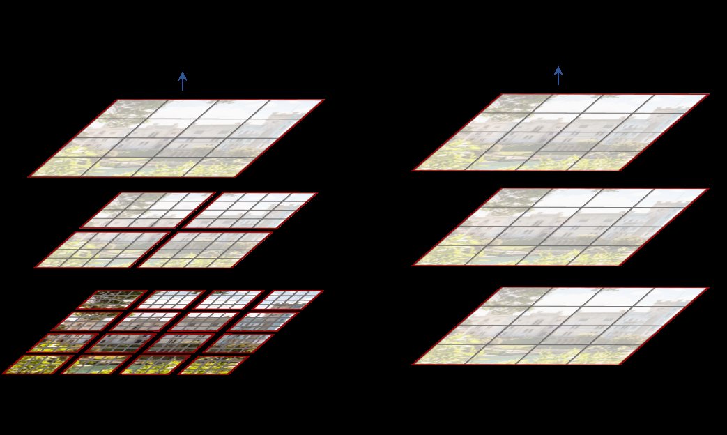
Figure 1: (a) The proposed Swin Transformer builds hierarchical feature maps by merging image patches (shown in gray) in deeper layers and has linear computation complexity to input image size due to computation of self-attention only within each local window (shown in red). It can thus serve as a general-purpose backbone for both image classification and dense recognition tasks. (b) In contrast, previous vision Transformers [20] produce feature maps of a single low resolution and have quadratic computation complexity to input image size due to computation of self-attention globally.
图 1:(a) 所提出的 Swin Transformer 通过在更深的层中合并图像 patch(灰色所示)构建层次化特征图,并且由于自注意力只在每个局部窗口(红色所示)内计算,对输入图像尺寸具有线性计算复杂度。因此它可作为图像分类与密集识别任务的通用骨干。(b) 相比之下,此前的视觉 Transformer [20] 产生单一低分辨率特征图,并且由于全局计算自注意力,对输入图像尺寸具有二次计算复杂度。
Modeling in computer vision has long been dominated by convolutional neural networks (CNNs). Beginning with AlexNet [39] and its revolutionary performance on the ImageNet image classification challenge, CNN architectures have evolved to become increasingly powerful through greater scale [30, 76], more extensive connections [34], and more sophisticated forms of convolution [70, 18, 84]. With CNNs serving as backbone networks for a variety of vision tasks, these architectural advances have led to performance improvements that have broadly lifted the entire field.
计算机视觉中的建模长期由卷积神经网络(CNN)主导。自 AlexNet [39] 及其在 ImageNet 图像分类挑战上的革命性表现开始,CNN 架构通过更大的规模 [30, 76]、更广泛的连接 [34] 以及更精巧的卷积形式 [70, 18, 84] 变得日益强大。随着 CNN 成为各类视觉任务的骨干网络,这些架构进展带来的性能提升广泛推动了整个领域。
On the other hand, the evolution of network architectures in natural language processing (NLP) has taken a different path, where the prevalent architecture today is instead the Transformer [64]. Designed for sequence modeling and transduction tasks, the Transformer is notable for its use of attention to model long-range dependencies in the data. Its tremendous success in the language domain has led researchers to investigate its adaptation to computer vision, where it has recently demonstrated promising results on certain tasks, specifically image classification [20] and joint vision-language modeling [47].
另一方面,自然语言处理(NLP)中网络架构的演进走了一条不同的道路,今天的主流架构反而是 Transformer [64]。Transformer 面向序列建模与转导任务,其显著特点是用注意力对数据中的长程依赖建模。它在语言领域的巨大成功促使研究者探索将其迁移到计算机视觉,并已在某些任务上展现出有希望的结果,特别是图像分类 [20] 以及联合视觉—语言建模 [47]。
In this paper, we seek to expand the applicability of Transformer such that it can serve as a general-purpose backbone for computer vision, as it does for NLP and as CNNs do in vision. We observe that significant challenges in transferring its high performance in the language domain to the visual domain can be explained by differences between the two modalities. One of these differences involves scale. Unlike the word tokens that serve as the basic elements of processing in language Transformers, visual elements can vary substantially in scale, a problem that receives attention in tasks such as object detection [42, 53, 54]. In existing Transformer-based models [64, 20], tokens are all of a fixed scale, a property unsuitable for these vision applications. Another difference is the much higher resolution of pixels in images compared to words in passages of text. There exist many vision tasks such as semantic segmentation that require dense prediction at the pixel level, and this would be intractable for Transformer on high-resolution images, as the computational complexity of its self-attention is quadratic to image size. To overcome these issues, we propose a general-purpose Transformer backbone, called Swin Transformer, which constructs hierarchical feature maps and has linear computational complexity to image size. As illustrated in Figure 1(a), Swin Transformer constructs a hierarchical representation by starting from small-sized patches (outlined in gray) and gradually merging neighboring patches in deeper Transformer layers. With these hierarchical feature maps, the Swin Transformer model can conveniently leverage advanced techniques for dense prediction such as feature pyramid networks (FPN) [42] or U-Net [51]. The linear computational complexity is achieved by computing self-attention locally within non-overlapping windows that partition an image (outlined in red). The number of patches in each window is fixed, and thus the complexity becomes linear to image size. These merits make Swin Transformer suitable as a general-purpose backbone for various vision tasks, in contrast to previous Transformer based architectures [20] which produce feature maps of a single resolution and have quadratic complexity.
在本文中,我们试图扩展 Transformer 的适用性,使其能像在 NLP 中那样、也像 CNN 在视觉中那样,成为计算机视觉的通用骨干。我们观察到,将其在语言领域的高性能迁移到视觉领域的主要挑战,可以由两种模态之间的差异来解释。差异之一涉及尺度。与语言 Transformer 中作为基本处理单元的词 token 不同,视觉元素的尺度可以有很大变化,这一问题在目标检测等任务中受到关注 [42, 53, 54]。在现有基于 Transformer 的模型 [64, 20] 中,token 都是固定尺度,这一属性不适合这些视觉应用。另一差异是图像中像素的分辨率远高于文本段落中的词。存在许多需要像素级密集预测的视觉任务,例如语义分割;这对高分辨率图像上的 Transformer 将难以承受,因为其自注意力的计算复杂度对图像尺寸是二次的。为克服这些问题,我们提出一种通用 Transformer 骨干,称为 Swin Transformer,它构建层次化特征图,并且对图像尺寸具有线性计算复杂度。如图 1(a) 所示,Swin Transformer 从较小尺寸的 patch(灰色轮廓)出发,并在更深的 Transformer 层中逐渐合并相邻 patch,从而构建层次化表示。借助这些层次化特征图,Swin Transformer 模型可以方便地利用特征金字塔网络(FPN)[42] 或 U-Net [51] 等用于密集预测的先进技术。线性计算复杂度通过对划分图像的互不重叠窗口(红色轮廓)在局部计算自注意力来实现。每个窗口内的 patch 数固定,因此复杂度对图像尺寸变为线性。这些优点使 Swin Transformer 适合作为多种视觉任务的通用骨干,这与此前基于 Transformer 的架构 [20] 形成对比——后者产生单一分辨率的特征图,并具有二次复杂度。
A key design element of Swin Transformer is its shift of the window partition between consecutive self-attention layers, as illustrated in Figure 2. The shifted windows bridge the windows of the preceding layer, providing connections among them that significantly enhance modeling power (see Table 4). This strategy is also efficient in regards to real-world latency: all query patches within a window share the same key set[^1], which facilitates memory access in hardware. In contrast, earlier sliding window based self-attention approaches [33, 50] suffer from low latency on general hardware due to different key sets for different query pixels[^2]. Our experiments show that the proposed shifted window approach has much lower latency than the sliding window method, yet is similar in modeling power (see Tables 5 and 6). The shifted window approach also proves beneficial for all-MLP architectures [61].
Swin Transformer 的一个关键设计要素是在连续自注意力层之间对窗口划分做平移,如图 2 所示。平移后的窗口桥接了前一层的各个窗口,在它们之间提供连接,从而显著增强建模能力(见表 4)。这一策略在真实延迟方面也很高效:一个窗口内的所有查询 patch 共享同一套键集[^1],这有利于硬件中的内存访问。相比之下,早期基于滑动窗口的自注意力方法 [33, 50] 由于不同查询像素使用不同的键集,在通用硬件上延迟较高[^2]。我们的实验表明,所提出的平移窗口方法比滑动窗口方法延迟低得多,而建模能力相近(见表 5 与表 6)。平移窗口方法对全 MLP 架构 [61] 同样有益。
The proposed Swin Transformer achieves strong performance on the recognition tasks of image classification, object detection and semantic segmentation. It outperforms the ViT / DeiT [20, 63] and ResNe(X)t models [30, 70] significantly with similar latency on the three tasks. Its 58.7 box AP and 51.1 mask AP on the COCO test-dev set surpass the previous state-of-the-art results by +2.7 box AP (Copy-paste [26] without external data) and +2.6 mask AP (DetectoRS [46]). On ADE20K semantic segmentation, it obtains 53.5 mIoU on the val set, an improvement of +3.2 mIoU over the previous state-of-the-art (SETR [81]). It also achieves a top-1 accuracy of 87.3% on ImageNet-1K image classification.
所提出的 Swin Transformer 在图像分类、目标检测与语义分割等识别任务上取得了强劲性能。在相近延迟下,它在三项任务上显著优于 ViT / DeiT [20, 63] 以及 ResNe(X)t 模型 [30, 70]。它在 COCO test-dev 集上取得 58.7 box AP 与 51.1 mask AP,分别比此前最优结果高出 +2.7 box AP(Copy-paste [26],无外部数据)与 +2.6 mask AP(DetectoRS [46])。在 ADE20K 语义分割上,它在 val 集上取得 53.5 mIoU,比此前最优(SETR [81])提升 +3.2 mIoU。它在 ImageNet-1K 图像分类上还达到 87.3% 的 top-1 准确率。
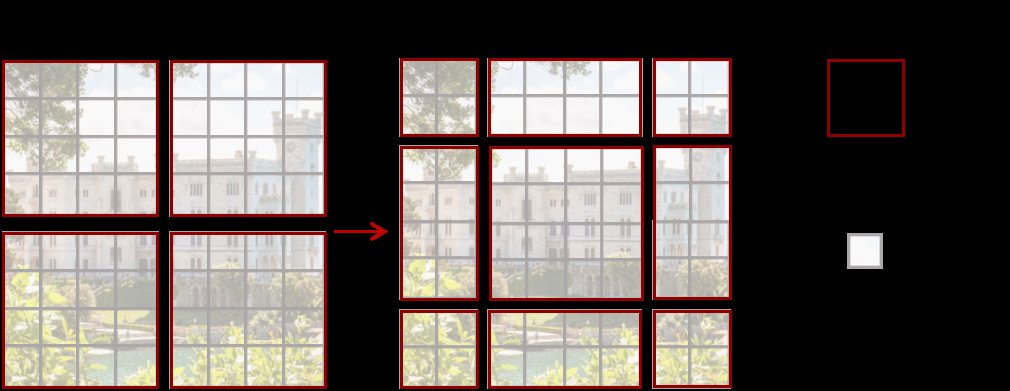
Figure 2: An illustration of the shifted window approach for computing self-attention in the proposed Swin Transformer architecture. In layer (left), a regular window partitioning scheme is adopted, and self-attention is computed within each window. In the next layer (right), the window partitioning is shifted, resulting in new windows. The self-attention computation in the new windows crosses the boundaries of the previous windows in layer , providing connections among them.
图 2:所提出的 Swin Transformer 架构中用于计算自注意力的平移窗口方法示意。在第 层(左),采用常规窗口划分方案,并在每个窗口内计算自注意力。在下一层 (右),窗口划分发生平移,形成新窗口。新窗口中的自注意力计算跨越了第 层先前窗口的边界,从而在它们之间提供连接。
It is our belief that a unified architecture across computer vision and natural language processing could benefit both fields, since it would facilitate joint modeling of visual and textual signals and the modeling knowledge from both domains can be more deeply shared. We hope that Swin Transformer’s strong performance on various vision problems can drive this belief deeper in the community and encourage unified modeling of vision and language signals.
我们相信,打通计算机视觉与自然语言处理的统一架构将使两个领域都受益,因为它便于对视觉与文本信号做联合建模,并且两个领域的建模知识可以更深入地共享。我们希望 Swin Transformer 在各类视觉问题上的强劲表现能推动这一信念在社区中更深扎根,并鼓励对视觉与语言信号的统一建模。
2 Related Work
2 相关工作
CNN and variants
CNN 及其变体
CNNs serve as the standard network model throughout computer vision. While the CNN has existed for several decades [40], it was not until the introduction of AlexNet [39] that the CNN took off and became mainstream. Since then, deeper and more effective convolutional neural architectures have been proposed to further propel the deep learning wave in computer vision, e.g., VGG [52], GoogleNet [57], ResNet [30], DenseNet [34], HRNet [65], and EfficientNet [58]. In addition to these architectural advances, there has also been much work on improving individual convolution layers, such as depth-wise convolution [70] and deformable convolution [18, 84]. While the CNN and its variants are still the primary backbone architectures for computer vision applications, we highlight the strong potential of Transformer-like architectures for unified modeling between vision and language. Our work achieves strong performance on several basic visual recognition tasks, and we hope it will contribute to a modeling shift.
CNN 是整个计算机视觉中的标准网络模型。尽管 CNN 已存在数十年 [40],但直到 AlexNet [39] 出现,CNN 才起飞并成为主流。此后,更深、更有效的卷积神经架构被提出,进一步推动了计算机视觉中的深度学习浪潮,例如 VGG [52]、GoogleNet [57]、ResNet [30]、DenseNet [34]、HRNet [65] 以及 EfficientNet [58]。除了这些架构进展,还有大量工作改进单个卷积层,例如深度可分离卷积 [70] 与可变形卷积 [18, 84]。虽然 CNN 及其变体仍是计算机视觉应用的主要骨干架构,我们强调类 Transformer 架构在视觉与语言统一建模方面的强大潜力。我们的工作在若干基本视觉识别任务上取得了强劲性能,希望能为建模范式的转变做出贡献。
Self-attention based backbone architectures
基于自注意力的骨干架构
Also inspired by the success of self-attention layers and Transformer architectures in the NLP field, some works employ self-attention layers to replace some or all of the spatial convolution layers in the popular ResNet [33, 50, 80]. In these works, the self-attention is computed within a local window of each pixel to expedite optimization [33], and they achieve slightly better accuracy/FLOPs trade-offs than the counterpart ResNet architecture. However, their costly memory access causes their actual latency to be significantly larger than that of the convolutional networks [33]. Instead of using sliding windows, we propose to shift windows between consecutive layers, which allows for a more efficient implementation in general hardware.
同样受自注意力层与 Transformer 架构在 NLP 领域成功的启发,一些工作用自注意力层替换流行 ResNet 中的部分或全部空间卷积层 [33, 50, 80]。在这些工作中,自注意力在每个像素的局部窗口内计算以加速优化 [33],它们相对对应的 ResNet 架构取得了略好的精度/FLOPs 权衡。然而,其高昂的内存访问导致实际延迟显著高于卷积网络 [33]。我们不使用滑动窗口,而是提出在连续层之间平移窗口,从而在通用硬件上实现更高效的实现。
Self-attention/Transformers to complement CNNs
用自注意力/Transformer 补充 CNN
Another line of work is to augment a standard CNN architecture with self-attention layers or Transformers. The self-attention layers can complement backbones [67, 7, 3, 71, 23, 74, 55] or head networks [32, 27] by providing the capability to encode distant dependencies or heterogeneous interactions. More recently, the encoder-decoder design in Transformer has been applied for the object detection and instance segmentation tasks [8, 13, 85, 56]. Our work explores the adaptation of Transformers for basic visual feature extraction and is complementary to these works.
另一条路线是用自注意力层或 Transformer 增强标准 CNN 架构。自注意力层可通过编码远距离依赖或异构交互来补充骨干 [67, 7, 3, 71, 23, 74, 55] 或头部网络 [32, 27]。最近,Transformer 中的编码器—解码器设计也被用于目标检测与实例分割任务 [8, 13, 85, 56]。我们的工作探索将 Transformer 适配于基本视觉特征提取,与这些工作互补。
Transformer based vision backbones
基于 Transformer 的视觉骨干
Most related to our work is the Vision Transformer (ViT) [20] and its follow-ups [63, 72, 15, 28, 66]. The pioneering work of ViT directly applies a Transformer architecture on non-overlapping medium-sized image patches for image classification. It achieves an impressive speed-accuracy trade-off on image classification compared to convolutional networks. While ViT requires large-scale training datasets (i.e., JFT-300M) to perform well, DeiT [63] introduces several training strategies that allow ViT to also be effective using the smaller ImageNet-1K dataset. The results of ViT on image classification are encouraging, but its architecture is unsuitable for use as a general-purpose backbone network on dense vision tasks or when the input image resolution is high, due to its low-resolution feature maps and the quadratic increase in complexity with image size. There are a few works applying ViT models to the dense vision tasks of object detection and semantic segmentation by direct upsampling or deconvolution but with relatively lower performance [2, 81]. Concurrent to our work are some that modify the ViT architecture [72, 15, 28] for better image classification. Empirically, we find our Swin Transformer architecture to achieve the best speed-accuracy trade-off among these methods on image classification, even though our work focuses on general-purpose performance rather than specifically on classification. Another concurrent work [66] explores a similar line of thinking to build multi-resolution feature maps on Transformers. Its complexity is still quadratic to image size, while ours is linear and also operates locally which has proven beneficial in modeling the high correlation in visual signals [36, 25, 41]. Our approach is both efficient and effective, achieving state-of-the-art accuracy on both COCO object detection and ADE20K semantic segmentation.
与我们工作最相关的是 Vision Transformer(ViT)[20] 及其后续工作 [63, 72, 15, 28, 66]。ViT 的开创性工作直接把 Transformer 架构应用到互不重叠的中等尺寸图像 patch 上做图像分类。相对卷积网络,它在图像分类上取得了令人印象深刻的速度—精度权衡。虽然 ViT 需要大规模训练数据集(即 JFT-300M)才能表现良好,DeiT [63] 引入了若干训练策略,使 ViT 在较小的 ImageNet-1K 数据集上也能有效。ViT 在图像分类上的结果令人鼓舞,但其架构不适合作为密集视觉任务或输入图像分辨率很高时的通用骨干网络,原因在于其特征图分辨率低,以及复杂度随图像尺寸二次增长。有少数工作通过对 ViT 模型直接上采样或反卷积来做目标检测与语义分割等密集视觉任务,但性能相对较低 [2, 81]。与我们同期的一些工作修改了 ViT 架构 [72, 15, 28] 以更好地做图像分类。经验上,我们发现我们的 Swin Transformer 架构在这些方法中取得了图像分类上最好的速度—精度权衡,尽管我们的工作关注通用性能而非专门面向分类。另一项同期工作 [66] 探索了类似思路,在 Transformer 上构建多分辨率特征图。其复杂度对图像尺寸仍是二次的,而我们的是线性的,并且在局部操作,这已被证明有利于对视觉信号中的高相关性建模 [36, 25, 41]。我们的方法既高效又有效,在 COCO 目标检测与 ADE20K 语义分割上都达到了当时最优精度。
3 Method
3 方法
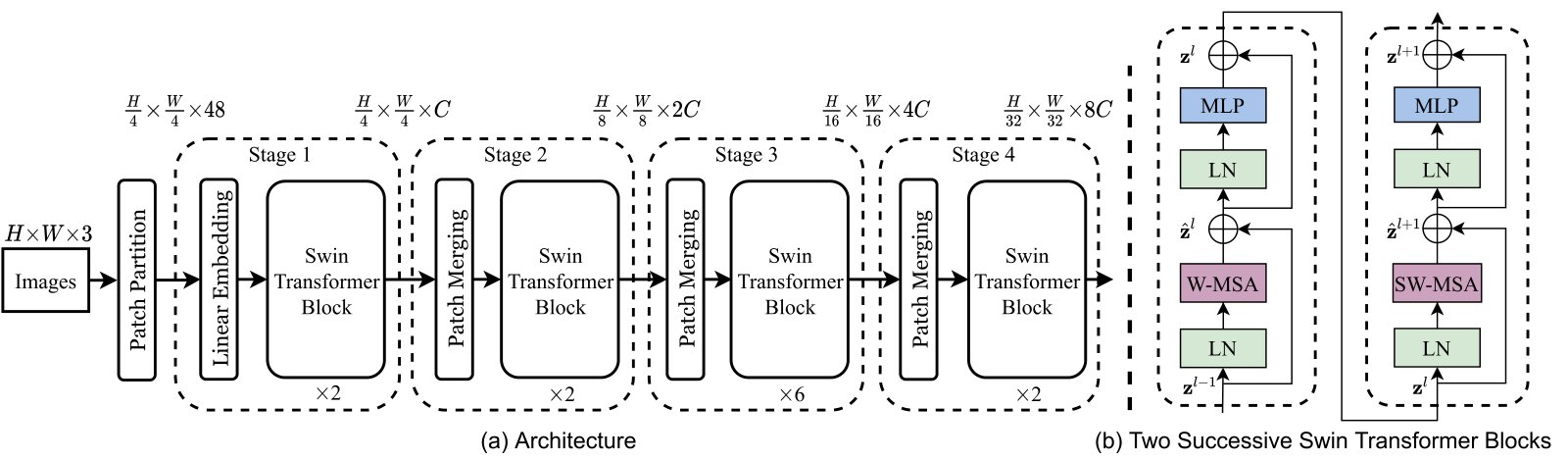
Figure 3: (a) The architecture of a Swin Transformer (Swin-T); (b) two successive Swin Transformer Blocks (notation presented with Eq. (3)). W-MSA and SW-MSA are multi-head self attention modules with regular and shifted windowing configurations, respectively.
图 3:(a) Swin Transformer(Swin-T)的架构;(b) 两个连续的 Swin Transformer Block(记号见式 (3))。W-MSA 与 SW-MSA 分别是采用常规与平移窗口配置的多头自注意力模块。
3.1 Overall Architecture
3.1 总体架构
An overview of the Swin Transformer architecture is presented in Figure 3, which illustrates the tiny version (Swin-T). It first splits an input RGB image into non-overlapping patches by a patch splitting module, like ViT. Each patch is treated as a “token” and its feature is set as a concatenation of the raw pixel RGB values. In our implementation, we use a patch size of and thus the feature dimension of each patch is . A linear embedding layer is applied on this raw-valued feature to project it to an arbitrary dimension (denoted as ).
图 3 给出了 Swin Transformer 架构总览,图示为微型版本(Swin-T)。它首先像 ViT 一样,由 patch 切分模块把输入 RGB 图像切成互不重叠的 patch。每个 patch 被当作一个 “token”,其特征设为原始像素 RGB 值的拼接。我们的实现使用 的 patch 大小,因此每个 patch 的特征维度为 。在该原始值特征上施加线性嵌入层,将其投影到任意维度(记为 )。
Several Transformer blocks with modified self-attention computation (Swin Transformer blocks) are applied on these patch tokens. The Transformer blocks maintain the number of tokens (), and together with the linear embedding are referred to as “Stage 1”.
随后在这些 patch token 上施加若干带有修改后自注意力计算的 Transformer 块(Swin Transformer 块)。Transformer 块保持 token 数量(),它们与线性嵌入一起称为 “Stage 1”。
To produce a hierarchical representation, the number of tokens is reduced by patch merging layers as the network gets deeper. The first patch merging layer concatenates the features of each group of neighboring patches, and applies a linear layer on the -dimensional concatenated features. This reduces the number of tokens by a multiple of ( downsampling of resolution), and the output dimension is set to . Swin Transformer blocks are applied afterwards for feature transformation, with the resolution kept at . This first block of patch merging and feature transformation is denoted as “Stage 2”. The procedure is repeated twice, as “Stage 3” and “Stage 4”, with output resolutions of and , respectively. These stages jointly produce a hierarchical representation, with the same feature map resolutions as those of typical convolutional networks, e.g., VGG [52] and ResNet [30]. As a result, the proposed architecture can conveniently replace the backbone networks in existing methods for various vision tasks.
为产生层次化表示,随着网络加深,token 数量由 patch 合并层减少。第一个 patch 合并层把每组 相邻 patch 的特征拼接起来,再对 维的拼接特征施加线性层。这将 token 数量减少 倍(分辨率 下采样),输出维度设为 。之后再施加 Swin Transformer 块做特征变换,分辨率保持为 。这第一段 patch 合并与特征变换记为 “Stage 2”。该过程再重复两次,称为 “Stage 3” 与 “Stage 4”,输出分辨率分别为 与 。这些 stage 共同产生层次化表示,其特征图分辨率与典型卷积网络相同,例如 VGG [52] 与 ResNet [30]。因此,所提出的架构可以方便地替换现有方法中的骨干网络,以用于各种视觉任务。
Swin Transformer block
Swin Transformer 块
Swin Transformer is built by replacing the standard multi-head self attention (MSA) module in a Transformer block by a module based on shifted windows (described in Section 3.2), with other layers kept the same. As illustrated in Figure 3(b), a Swin Transformer block consists of a shifted window based MSA module, followed by a 2-layer MLP with GELU non-linearity in between. A LayerNorm (LN) layer is applied before each MSA module and each MLP, and a residual connection is applied after each module.
Swin Transformer 通过把 Transformer 块中的标准多头自注意力(MSA)模块替换为基于平移窗口的模块(见第 3.2 节)来构建,其余层保持不变。如图 3(b) 所示,一个 Swin Transformer 块由一个基于平移窗口的 MSA 模块,后接一个中间带 GELU 非线性的 2 层 MLP 组成。在每个 MSA 模块与每个 MLP 之前施加 LayerNorm(LN),并在每个模块之后施加残差连接。
3.2 Shifted Window based Self-Attention
3.2 基于平移窗口的自注意力
The standard Transformer architecture [64] and its adaptation for image classification [20] both conduct global self-attention, where the relationships between a token and all other tokens are computed. The global computation leads to quadratic complexity with respect to the number of tokens, making it unsuitable for many vision problems requiring an immense set of tokens for dense prediction or to represent a high-resolution image.
标准 Transformer 架构 [64] 及其面向图像分类的适配 [20] 都进行全局自注意力,即计算一个 token 与所有其他 token 之间的关系。全局计算导致复杂度对 token 数量呈二次,使其不适合许多需要海量 token 做密集预测或表示高分辨率图像的视觉问题。
Self-attention in non-overlapped windows
互不重叠窗口中的自注意力
For efficient modeling, we propose to compute self-attention within local windows. The windows are arranged to evenly partition the image in a non-overlapping manner. Supposing each window contains patches, the computational complexity of a global MSA module and a window based one on an image of patches are[^3]:
为高效建模,我们提出在局部窗口内计算自注意力。窗口以互不重叠的方式均匀划分图像。假设每个窗口包含 个 patch,则在一幅 个 patch 的图像上,全局 MSA 模块与基于窗口的模块的计算复杂度分别为[^3]:
where the former is quadratic to patch number , and the latter is linear when is fixed (set to by default). Global self-attention computation is generally unaffordable for a large , while the window based self-attention is scalable.
其中前者对 patch 数 呈二次,后者在 固定时(默认设为 )呈线性。对很大的 ,全局自注意力计算通常难以承受,而基于窗口的自注意力则可扩展。
Shifted window partitioning in successive blocks
连续块中的平移窗口划分
The window-based self-attention module lacks connections across windows, which limits its modeling power. To introduce cross-window connections while maintaining the efficient computation of non-overlapping windows, we propose a shifted window partitioning approach which alternates between two partitioning configurations in consecutive Swin Transformer blocks.
基于窗口的自注意力模块缺乏跨窗口连接,限制了其建模能力。为在保持互不重叠窗口高效计算的同时引入跨窗口连接,我们提出一种平移窗口划分方法,在连续的 Swin Transformer 块中交替使用两种划分配置。
As illustrated in Figure 2, the first module uses a regular window partitioning strategy which starts from the top-left pixel, and the feature map is evenly partitioned into windows of size (). Then, the next module adopts a windowing configuration that is shifted from that of the preceding layer, by displacing the windows by pixels from the regularly partitioned windows.
如图 2 所示,第一个模块使用从左上角像素开始的常规窗口划分策略, 特征图被均匀划分为 个大小为 的窗口()。然后,下一个模块采用相对前一层平移后的窗口配置,把窗口从常规划分位置位移 个像素。
With the shifted window partitioning approach, consecutive Swin Transformer blocks are computed as
采用平移窗口划分方法后,连续的 Swin Transformer 块计算为
where and denote the output features of the (S)W-MSA module and the MLP module for block , respectively; W-MSA and SW-MSA denote window based multi-head self-attention using regular and shifted window partitioning configurations, respectively.
其中 与 分别表示第 个块中 (S)W-MSA 模块与 MLP 模块的输出特征;W-MSA 与 SW-MSA 分别表示使用常规与平移窗口划分配置的基于窗口的多头自注意力。
The shifted window partitioning approach introduces connections between neighboring non-overlapping windows in the previous layer and is found to be effective in image classification, object detection, and semantic segmentation, as shown in Table 4.
平移窗口划分方法在前一层的相邻互不重叠窗口之间引入了连接,并在图像分类、目标检测与语义分割上被证明有效,如表 4 所示。
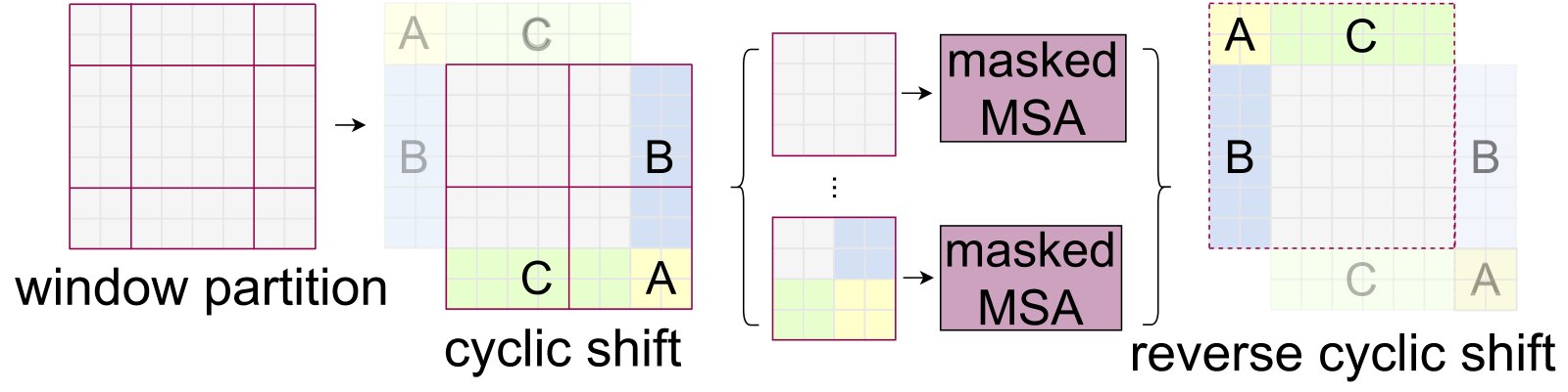
Figure 4: Illustration of an efficient batch computation approach for self-attention in shifted window partitioning.
图 4:平移窗口划分下自注意力的高效批次计算示意。
Efficient batch computation for shifted configuration
平移配置的高效批次计算
An issue with shifted window partitioning is that it will result in more windows, from to in the shifted configuration, and some of the windows will be smaller than [^4]. A naive solution is to pad the smaller windows to a size of and mask out the padded values when computing attention. When the number of windows in regular partitioning is small, e.g. , the increased computation with this naive solution is considerable (, which is 2.25 times greater). Here, we propose a more efficient batch computation approach by cyclic-shifting toward the top-left direction, as illustrated in Figure 4. After this shift, a batched window may be composed of several sub-windows that are not adjacent in the feature map, so a masking mechanism is employed to limit self-attention computation to within each sub-window. With the cyclic-shift, the number of batched windows remains the same as that of regular window partitioning, and thus is also efficient. The low latency of this approach is shown in Table 5.
平移窗口划分的一个问题是窗口数会从 增加到平移配置中的 ,并且有些窗口会小于 [^4]。一种朴素做法是把较小窗口填充到 ,并在计算注意力时把填充值 mask 掉。当常规划分中的窗口数较少时,例如 ,这种朴素做法带来的计算增加相当可观(,即增大 2.25 倍)。这里我们提出一种更高效的批次计算方法:向左上方向做循环移位,如图 4 所示。该移位之后,一个批次窗口可能由特征图上并不相邻的若干子窗口组成,因此采用 mask 机制把自注意力计算限制在每个子窗口内。借助循环移位,批次窗口数与常规划分保持相同,因而同样高效。表 5 展示了该方法的低延迟。
Relative position bias
相对位置偏置
In computing self-attention, we follow [49, 1, 32, 33] by including a relative position bias to each head in computing similarity:
在计算自注意力时,我们沿用 [49, 1, 32, 33],在每个头计算相似度时加入相对位置偏置 :
where are the query, key and value matrices; is the query/key dimension, and is the number of patches in a window. Since the relative position along each axis lies in the range , we parameterize a smaller-sized bias matrix , and values in are taken from .
其中 为 query、key 与 value 矩阵; 为 query/key 维度, 为窗口内的 patch 数。由于沿每个轴的相对位置落在 范围内,我们参数化一个更小尺寸的偏置矩阵 , 中的值取自 。
We observe significant improvements over counterparts without this bias term or that use absolute position embedding, as shown in Table 4. Further adding absolute position embedding to the input as in [20] drops performance slightly, thus it is not adopted in our implementation.
我们观察到,相对无该偏置项或使用绝对位置嵌入的对照,性能有显著提升,如表 4 所示。进一步像 [20] 那样在输入上再加绝对位置嵌入会略微下降性能,因此我们的实现未采用。
The learnt relative position bias in pre-training can be also used to initialize a model for fine-tuning with a different window size through bi-cubic interpolation [20, 63].
预训练中学到的相对位置偏置也可通过双三次插值 [20, 63] 初始化用于不同窗口大小的微调模型。
3.3 Architecture Variants
3.3 架构变体
We build our base model, called Swin-B, to have of model size and computation complexity similar to ViT-B/DeiT-B. We also introduce Swin-T, Swin-S and Swin-L, which are versions of about , and the model size and computational complexity, respectively. Note that the complexity of Swin-T and Swin-S are similar to those of ResNet-50 (DeiT-S) and ResNet-101, respectively. The window size is set to by default. The query dimension of each head is , and the expansion layer of each MLP is , for all experiments. The architecture hyper-parameters of these model variants are:
我们构建基础模型,称为 Swin-B,使其模型规模与计算复杂度与 ViT-B/DeiT-B 相近。我们还引入 Swin-T、Swin-S 与 Swin-L,其模型规模与计算复杂度大约分别为基础模型的 、 与 。注意 Swin-T 与 Swin-S 的复杂度分别与 ResNet-50(DeiT-S)和 ResNet-101 相近。窗口大小默认设为 。所有实验中,每个头的 query 维度为 ,每个 MLP 的扩展层为 。这些模型变体的架构超参数为:
- • Swin-T: , layer numbers =
- • Swin-S: , layer numbers =
- • Swin-B: , layer numbers =
- • Swin-L: , layer numbers =
- • Swin-T:,层数 =
- • Swin-S:,层数 =
- • Swin-B:,层数 =
- • Swin-L:,层数 =
where is the channel number of the hidden layers in the first stage. The model size, theoretical computational complexity (FLOPs), and throughput of the model variants for ImageNet image classification are listed in Table 1.
其中 是第一阶段隐层的通道数。各模型变体用于 ImageNet 图像分类的模型规模、理论计算复杂度(FLOPs)与吞吐量列于表 1。
4 Experiments
4 实验
We conduct experiments on ImageNet-1K image classification [19], COCO object detection [43], and ADE20K semantic segmentation [83]. In the following, we first compare the proposed Swin Transformer architecture with the previous state-of-the-arts on the three tasks. Then, we ablate the important design elements of Swin Transformer.
我们在 ImageNet-1K 图像分类 [19]、COCO 目标检测 [43] 与 ADE20K 语义分割 [83] 上进行实验。下文先在三项任务上把所提出的 Swin Transformer 架构与此前的最优方法比较,再消融 Swin Transformer 的重要设计要素。
4.1 Image Classification on ImageNet-1K
4.1 ImageNet-1K 图像分类
Settings
设置
For image classification, we benchmark the proposed Swin Transformer on ImageNet-1K [19], which contains 1.28M training images and 50K validation images from 1,000 classes. The top-1 accuracy on a single crop is reported. We consider two training settings:
对于图像分类,我们在 ImageNet-1K [19] 上评测所提出的 Swin Transformer,该数据集包含来自 1000 类的 128 万训练图像与 5 万验证图像。报告单裁剪的 top-1 准确率。我们考虑两种训练设置:
- • Regular ImageNet-1K training. This setting mostly follows [63]. We employ an AdamW [37] optimizer for 300 epochs using a cosine decay learning rate scheduler and 20 epochs of linear warm-up. A batch size of 1024, an initial learning rate of 0.001, and a weight decay of 0.05 are used. We include most of the augmentation and regularization strategies of [63] in training, except for repeated augmentation [31] and EMA [45], which do not enhance performance. Note that this is contrary to [63] where repeated augmentation is crucial to stabilize the training of ViT.
- • Pre-training on ImageNet-22K and fine-tuning on ImageNet-1K. We also pre-train on the larger ImageNet-22K dataset, which contains 14.2 million images and 22K classes. We employ an AdamW optimizer for 90 epochs using a linear decay learning rate scheduler with a 5-epoch linear warm-up. A batch size of 4096, an initial learning rate of 0.001, and a weight decay of 0.01 are used. In ImageNet-1K fine-tuning, we train the models for 30 epochs with a batch size of 1024, a constant learning rate of , and a weight decay of .
- • 常规 ImageNet-1K 训练。该设置大体遵循 [63]。我们使用 AdamW [37] 优化器训练 300 个 epoch,采用余弦衰减学习率调度与 20 个 epoch 的线性预热。批大小为 1024,初始学习率 0.001,权重衰减 0.05。训练中纳入 [63] 的大多数增强与正则策略,但不包括重复增强 [31] 与 EMA [45],因为它们并未提升性能。注意这与 [63] 相反——在那里重复增强对稳定 ViT 训练至关重要。
- • 在 ImageNet-22K 上预训练并在 ImageNet-1K 上微调。我们还在更大的 ImageNet-22K 数据集上预训练,该数据集包含 1420 万图像与 22K 类。使用 AdamW 优化器训练 90 个 epoch,采用带 5 个 epoch 线性预热的线性衰减学习率调度。批大小 4096,初始学习率 0.001,权重衰减 0.01。在 ImageNet-1K 微调中,训练 30 个 epoch,批大小 1024,恒定学习率 ,权重衰减 。
Results with regular ImageNet-1K training
常规 ImageNet-1K 训练的结果
Table 1(a) presents comparisons to other backbones, including both Transformer-based and ConvNet-based, using regular ImageNet-1K training.
表 1(a) 给出了与其他骨干的比较,包括基于 Transformer 与基于 ConvNet 的骨干,均使用常规 ImageNet-1K 训练。
Compared to the previous state-of-the-art Transformer-based architecture, i.e. DeiT [63], Swin Transformers noticeably surpass the counterpart DeiT architectures with similar complexities: +1.5% for Swin-T (81.3%) over DeiT-S (79.8%) using 2242 input, and +1.5%/1.4% for Swin-B (83.3%/84.5%) over DeiT-B (81.8%/83.1%) using 2242/3842 input, respectively.
相对此前最优的基于 Transformer 的架构,即 DeiT [63],Swin Transformer 在相近复杂度下明显超过对应的 DeiT:224² 输入下 Swin-T(81.3%)相对 DeiT-S(79.8%)高 +1.5%;224²/384² 输入下 Swin-B(83.3%/84.5%)相对 DeiT-B(81.8%/83.1%)分别高 +1.5%/1.4%。
Compared with the state-of-the-art ConvNets, i.e. RegNet [48] and EfficientNet [58], the Swin Transformer achieves a slightly better speed-accuracy trade-off. Noting that while RegNet [48] and EfficientNet [58] are obtained via a thorough architecture search, the proposed Swin Transformer is adapted from the standard Transformer and has strong potential for further improvement.
相对最优的 ConvNet,即 RegNet [48] 与 EfficientNet [58],Swin Transformer 取得略好的速度—精度权衡。需要指出的是,RegNet [48] 与 EfficientNet [58] 是通过充分的架构搜索得到的,而所提出的 Swin Transformer 由标准 Transformer 适配而来,仍有很大进一步改进空间。
Results with ImageNet-22K pre-training
ImageNet-22K 预训练的结果
We also pre-train the larger-capacity Swin-B and Swin-L on ImageNet-22K. Results fine-tuned on ImageNet-1K image classification are shown in Table 1(b). For Swin-B, the ImageNet-22K pre-training brings 1.8%1.9% gains over training on ImageNet-1K from scratch. Compared with the previous best results for ImageNet-22K pre-training, our models achieve significantly better speed-accuracy trade-offs: Swin-B obtains 86.4% top-1 accuracy, which is 2.4% higher than that of ViT with similar inference throughput (84.7 vs. 85.9 images/sec) and slightly lower FLOPs (47.0G vs. 55.4G). The larger Swin-L model achieves 87.3% top-1 accuracy, +0.9% better than that of the Swin-B model.
我们还在 ImageNet-22K 上预训练更大容量的 Swin-B 与 Swin-L。在 ImageNet-1K 上微调的图像分类结果见表 1(b)。对 Swin-B,ImageNet-22K 预训练相对从 ImageNet-1K 从头训练带来 1.8%~1.9% 的收益。相对此前 ImageNet-22K 预训练的最佳结果,我们的模型取得显著更好的速度—精度权衡:Swin-B 取得 86.4% top-1 准确率,比相近推理吞吐量的 ViT 高 2.4%(84.7 vs. 85.9 图像/秒),FLOPs 略低(47.0G vs. 55.4G)。更大的 Swin-L 模型达到 87.3% top-1 准确率,比 Swin-B 高 +0.9%。
| (a) Regular ImageNet-1K trained models | |||||||||||
|---|---|---|---|---|---|---|---|---|---|---|---|
| method | image size | image | size | #param. | FLOPs | throughput (image / s) | throughput | (image / s) | ImageNet top-1 acc. | ImageNet | top-1 acc. |
| image | |||||||||||
| size | |||||||||||
| throughput | |||||||||||
| (image / s) | |||||||||||
| ImageNet | |||||||||||
| top-1 acc. | |||||||||||
| RegNetY-4G [48] | 2242 | 21M | 4.0G | 1156.7 | 80.0 | ||||||
| RegNetY-8G [48] | 2242 | 39M | 8.0G | 591.6 | 81.7 | ||||||
| RegNetY-16G [48] | 2242 | 84M | 16.0G | 334.7 | 82.9 | ||||||
| EffNet-B3 [58] | 3002 | 12M | 1.8G | 732.1 | 81.6 | ||||||
| EffNet-B4 [58] | 3802 | 19M | 4.2G | 349.4 | 82.9 | ||||||
| EffNet-B5 [58] | 4562 | 30M | 9.9G | 169.1 | 83.6 | ||||||
| EffNet-B6 [58] | 5282 | 43M | 19.0G | 96.9 | 84.0 | ||||||
| EffNet-B7 [58] | 6002 | 66M | 37.0G | 55.1 | 84.3 | ||||||
| ViT-B/16 [20] | 3842 | 86M | 55.4G | 85.9 | 77.9 | ||||||
| ViT-L/16 [20] | 3842 | 307M | 190.7G | 27.3 | 76.5 | ||||||
| DeiT-S [63] | 2242 | 22M | 4.6G | 940.4 | 79.8 | ||||||
| DeiT-B [63] | 2242 | 86M | 17.5G | 292.3 | 81.8 | ||||||
| DeiT-B [63] | 3842 | 86M | 55.4G | 85.9 | 83.1 | ||||||
| Swin-T | 2242 | 29M | 4.5G | 755.2 | 81.3 | ||||||
| Swin-S | 2242 | 50M | 8.7G | 436.9 | 83.0 | ||||||
| Swin-B | 2242 | 88M | 15.4G | 278.1 | 83.5 | ||||||
| Swin-B | 3842 | 88M | 47.0G | 84.7 | 84.5 | ||||||
| (b) ImageNet-22K pre-trained models | |||||||||||
| method | image size | image | size | #param. | FLOPs | throughput (image / s) | throughput | (image / s) | ImageNet top-1 acc. | ImageNet | top-1 acc. |
| image | |||||||||||
| size | |||||||||||
| throughput | |||||||||||
| (image / s) | |||||||||||
| ImageNet | |||||||||||
| top-1 acc. | |||||||||||
| R-101x3 [38] | 3842 | 388M | 204.6G | - | 84.4 | ||||||
| R-152x4 [38] | 4802 | 937M | 840.5G | - | 85.4 | ||||||
| ViT-B/16 [20] | 3842 | 86M | 55.4G | 85.9 | 84.0 | ||||||
| ViT-L/16 [20] | 3842 | 307M | 190.7G | 27.3 | 85.2 | ||||||
| Swin-B | 2242 | 88M | 15.4G | 278.1 | 85.2 | ||||||
| Swin-B | 3842 | 88M | 47.0G | 84.7 | 86.4 | ||||||
| Swin-L | 3842 | 197M | 103.9G | 42.1 | 87.3 |
| image |
|---|
| size |
| throughput |
|---|
| (image / s) |
| ImageNet |
|---|
| top-1 acc. |
| image |
|---|
| size |
| throughput |
|---|
| (image / s) |
| ImageNet |
|---|
| top-1 acc. |
Table 1: Comparison of different backbones on ImageNet-1K classification. Throughput is measured using the GitHub repository of [68] and a V100 GPU, following [63].
| (a) Regular ImageNet-1K trained models | |||||||||||
|---|---|---|---|---|---|---|---|---|---|---|---|
| method | image size | image | size | #param. | FLOPs | throughput (image / s) | throughput | (image / s) | ImageNet top-1 acc. | ImageNet | top-1 acc. |
| image | |||||||||||
| size | |||||||||||
| throughput | |||||||||||
| (image / s) | |||||||||||
| ImageNet | |||||||||||
| top-1 acc. | |||||||||||
| RegNetY-4G [48] | 2242 | 21M | 4.0G | 1156.7 | 80.0 | ||||||
| RegNetY-8G [48] | 2242 | 39M | 8.0G | 591.6 | 81.7 | ||||||
| RegNetY-16G [48] | 2242 | 84M | 16.0G | 334.7 | 82.9 | ||||||
| EffNet-B3 [58] | 3002 | 12M | 1.8G | 732.1 | 81.6 | ||||||
| EffNet-B4 [58] | 3802 | 19M | 4.2G | 349.4 | 82.9 | ||||||
| EffNet-B5 [58] | 4562 | 30M | 9.9G | 169.1 | 83.6 | ||||||
| EffNet-B6 [58] | 5282 | 43M | 19.0G | 96.9 | 84.0 | ||||||
| EffNet-B7 [58] | 6002 | 66M | 37.0G | 55.1 | 84.3 | ||||||
| ViT-B/16 [20] | 3842 | 86M | 55.4G | 85.9 | 77.9 | ||||||
| ViT-L/16 [20] | 3842 | 307M | 190.7G | 27.3 | 76.5 | ||||||
| DeiT-S [63] | 2242 | 22M | 4.6G | 940.4 | 79.8 | ||||||
| DeiT-B [63] | 2242 | 86M | 17.5G | 292.3 | 81.8 | ||||||
| DeiT-B [63] | 3842 | 86M | 55.4G | 85.9 | 83.1 | ||||||
| Swin-T | 2242 | 29M | 4.5G | 755.2 | 81.3 | ||||||
| Swin-S | 2242 | 50M | 8.7G | 436.9 | 83.0 | ||||||
| Swin-B | 2242 | 88M | 15.4G | 278.1 | 83.5 | ||||||
| Swin-B | 3842 | 88M | 47.0G | 84.7 | 84.5 | ||||||
| (b) ImageNet-22K pre-trained models | |||||||||||
| method | image size | image | size | #param. | FLOPs | throughput (image / s) | throughput | (image / s) | ImageNet top-1 acc. | ImageNet | top-1 acc. |
| image | |||||||||||
| size | |||||||||||
| throughput | |||||||||||
| (image / s) | |||||||||||
| ImageNet | |||||||||||
| top-1 acc. | |||||||||||
| R-101x3 [38] | 3842 | 388M | 204.6G | - | 84.4 | ||||||
| R-152x4 [38] | 4802 | 937M | 840.5G | - | 85.4 | ||||||
| ViT-B/16 [20] | 3842 | 86M | 55.4G | 85.9 | 84.0 | ||||||
| ViT-L/16 [20] | 3842 | 307M | 190.7G | 27.3 | 85.2 | ||||||
| Swin-B | 2242 | 88M | 15.4G | 278.1 | 85.2 | ||||||
| Swin-B | 3842 | 88M | 47.0G | 84.7 | 86.4 | ||||||
| Swin-L | 3842 | 197M | 103.9G | 42.1 | 87.3 |
| image |
|---|
| size |
| throughput |
|---|
| (image / s) |
| ImageNet |
|---|
| top-1 acc. |
| image |
|---|
| size |
| throughput |
|---|
| (image / s) |
| ImageNet |
|---|
| top-1 acc. |
表 1:不同骨干在 ImageNet-1K 分类上的比较。吞吐量用 [68] 的 GitHub 仓库与一块 V100 GPU 测量,遵循 [63]。
4.2 Object Detection on COCO
4.2 COCO 目标检测
Settings
设置
Object detection and instance segmentation experiments are conducted on COCO 2017, which contains 118K training, 5K validation and 20K test-dev images. An ablation study is performed using the validation set, and a system-level comparison is reported on test-dev. For the ablation study, we consider four typical object detection frameworks: Cascade Mask R-CNN [29, 6], ATSS [79], RepPoints v2 [12], and Sparse RCNN [56] in mmdetection [10]. For these four frameworks, we utilize the same settings: multi-scale training [8, 56] (resizing the input such that the shorter side is between 480 and 800 while the longer side is at most 1333), AdamW [44] optimizer (initial learning rate of 0.0001, weight decay of 0.05, and batch size of 16), and 3x schedule (36 epochs). For system-level comparison, we adopt an improved HTC [9] (denoted as HTC++) with instaboost [22], stronger multi-scale training [7], 6x schedule (72 epochs), soft-NMS [5], and ImageNet-22K pre-trained model as initialization.
目标检测与实例分割实验在 COCO 2017 上进行,包含 118K 训练、5K 验证与 20K test-dev 图像。消融研究在验证集上进行,系统级比较在 test-dev 上报告。对消融研究,我们在 mmdetection [10] 中考虑四种典型目标检测框架:Cascade Mask R-CNN [29, 6]、ATSS [79]、RepPoints v2 [12] 与 Sparse RCNN [56]。对这四个框架,我们使用相同设置:多尺度训练 [8, 56](调整输入使较短边在 480 与 800 之间,较长边至多 1333)、AdamW [44] 优化器(初始学习率 0.0001,权重衰减 0.05,批大小 16)以及 3x 日程(36 个 epoch)。对系统级比较,我们采用改进的 HTC [9](记为 HTC++),配合 instaboost [22]、更强的多尺度训练 [7]、6x 日程(72 个 epoch)、soft-NMS [5],并以 ImageNet-22K 预训练模型作为初始化。
We compare our Swin Transformer to standard ConvNets, i.e. ResNe(X)t, and previous Transformer networks, e.g. DeiT. The comparisons are conducted by changing only the backbones with other settings unchanged. Note that while Swin Transformer and ResNe(X)t are directly applicable to all the above frameworks because of their hierarchical feature maps, DeiT only produces a single resolution of feature maps and cannot be directly applied. For fair comparison, we follow [81] to construct hierarchical feature maps for DeiT using deconvolution layers.
我们将 Swin Transformer 与标准 ConvNet(即 ResNe(X)t)以及此前的 Transformer 网络(例如 DeiT)进行比较。比较时只更换骨干,其余设置不变。注意由于具有层次化特征图,Swin Transformer 与 ResNe(X)t 可直接用于上述所有框架,而 DeiT 只产生单一分辨率特征图,不能直接应用。为公平比较,我们遵循 [81],用反卷积层为 DeiT 构造层次化特征图。
| (a) Various frameworks | |||||||
|---|---|---|---|---|---|---|---|
| Method | Backbone | AP | AP | AP | #param. | FLOPs | FPS |
| Cascade Mask R-CNN | R-50 | 46.3 | 64.3 | 50.5 | 82M | 739G | 18.0 |
| Swin-T | 50.5 | 69.3 | 54.9 | 86M | 745G | 15.3 | |
| ATSS | R-50 | 43.5 | 61.9 | 47.0 | 32M | 205G | 28.3 |
| Swin-T | 47.2 | 66.5 | 51.3 | 36M | 215G | 22.3 | |
| RepPointsV2 | R-50 | 46.5 | 64.6 | 50.3 | 42M | 274G | 13.6 |
| Swin-T | 50.0 | 68.5 | 54.2 | 45M | 283G | 12.0 | |
| Sparse R-CNN | R-50 | 44.5 | 63.4 | 48.2 | 106M | 166G | 21.0 |
| Swin-T | 47.9 | 67.3 | 52.3 | 110M | 172G | 18.4 |
| (b) Various backbones w. Cascade Mask R-CNN | |||||||||
|---|---|---|---|---|---|---|---|---|---|
| AP | AP | AP | AP | AP | AP | param | FLOPs | FPS | |
| DeiT-S*†* | 48.0 | 67.2 | 51.7 | 41.4 | 64.2 | 44.3 | 80M | 889G | 10.4 |
| R50 | 46.3 | 64.3 | 50.5 | 40.1 | 61.7 | 43.4 | 82M | 739G | 18.0 |
| Swin-T | 50.5 | 69.3 | 54.9 | 43.7 | 66.6 | 47.1 | 86M | 745G | 15.3 |
| X101-32 | 48.1 | 66.5 | 52.4 | 41.6 | 63.9 | 45.2 | 101M | 819G | 12.8 |
| Swin-S | 51.8 | 70.4 | 56.3 | 44.7 | 67.9 | 48.5 | 107M | 838G | 12.0 |
| X101-64 | 48.3 | 66.4 | 52.3 | 41.7 | 64.0 | 45.1 | 140M | 972G | 10.4 |
| Swin-B | 51.9 | 70.9 | 56.5 | 45.0 | 68.4 | 48.7 | 145M | 982G | 11.6 |
| (c) System-level Comparison | ||||||
|---|---|---|---|---|---|---|
| Method | mini-val | test-dev | #param. | FLOPs | ||
| AP | AP | AP | AP | |||
| RepPointsV2* [12] | - | - | 52.1 | - | - | - |
| GCNet* [7] | 51.8 | 44.7 | 52.3 | 45.4 | - | 1041G |
| RelationNet++* [13] | - | - | 52.7 | - | - | - |
| SpineNet-190 [21] | 52.6 | - | 52.8 | - | 164M | 1885G |
| ResNeSt-200* [78] | 52.5 | - | 53.3 | 47.1 | - | - |
| EfficientDet-D7 [59] | 54.4 | - | 55.1 | - | 77M | 410G |
| DetectoRS* [46] | - | - | 55.7 | 48.5 | - | - |
| YOLOv4 P7* [4] | - | - | 55.8 | - | - | - |
| Copy-paste [26] | 55.9 | 47.2 | 56.0 | 47.4 | 185M | 1440G |
| X101-64 (HTC++) | 52.3 | 46.0 | - | - | 155M | 1033G |
| Swin-B (HTC++) | 56.4 | 49.1 | - | - | 160M | 1043G |
| Swin-L (HTC++) | 57.1 | 49.5 | 57.7 | 50.2 | 284M | 1470G |
| Swin-L (HTC++)* | 58.0 | 50.4 | 58.7 | 51.1 | 284M | - |
Table 2: Results on COCO object detection and instance segmentation. *†*denotes that additional decovolution layers are used to produce hierarchical feature maps. * indicates multi-scale testing.
| (a) Various frameworks | |||||||
|---|---|---|---|---|---|---|---|
| Method | Backbone | AP | AP | AP | #param. | FLOPs | FPS |
| Cascade Mask R-CNN | R-50 | 46.3 | 64.3 | 50.5 | 82M | 739G | 18.0 |
| Swin-T | 50.5 | 69.3 | 54.9 | 86M | 745G | 15.3 | |
| ATSS | R-50 | 43.5 | 61.9 | 47.0 | 32M | 205G | 28.3 |
| Swin-T | 47.2 | 66.5 | 51.3 | 36M | 215G | 22.3 | |
| RepPointsV2 | R-50 | 46.5 | 64.6 | 50.3 | 42M | 274G | 13.6 |
| Swin-T | 50.0 | 68.5 | 54.2 | 45M | 283G | 12.0 | |
| Sparse R-CNN | R-50 | 44.5 | 63.4 | 48.2 | 106M | 166G | 21.0 |
| Swin-T | 47.9 | 67.3 | 52.3 | 110M | 172G | 18.4 |
| (b) Various backbones w. Cascade Mask R-CNN | |||||||||
|---|---|---|---|---|---|---|---|---|---|
| AP | AP | AP | AP | AP | AP | param | FLOPs | FPS | |
| DeiT-S*†* | 48.0 | 67.2 | 51.7 | 41.4 | 64.2 | 44.3 | 80M | 889G | 10.4 |
| R50 | 46.3 | 64.3 | 50.5 | 40.1 | 61.7 | 43.4 | 82M | 739G | 18.0 |
| Swin-T | 50.5 | 69.3 | 54.9 | 43.7 | 66.6 | 47.1 | 86M | 745G | 15.3 |
| X101-32 | 48.1 | 66.5 | 52.4 | 41.6 | 63.9 | 45.2 | 101M | 819G | 12.8 |
| Swin-S | 51.8 | 70.4 | 56.3 | 44.7 | 67.9 | 48.5 | 107M | 838G | 12.0 |
| X101-64 | 48.3 | 66.4 | 52.3 | 41.7 | 64.0 | 45.1 | 140M | 972G | 10.4 |
| Swin-B | 51.9 | 70.9 | 56.5 | 45.0 | 68.4 | 48.7 | 145M | 982G | 11.6 |
| (c) System-level Comparison | ||||||
|---|---|---|---|---|---|---|
| Method | mini-val | test-dev | #param. | FLOPs | ||
| AP | AP | AP | AP | |||
| RepPointsV2* [12] | - | - | 52.1 | - | - | - |
| GCNet* [7] | 51.8 | 44.7 | 52.3 | 45.4 | - | 1041G |
| RelationNet++* [13] | - | - | 52.7 | - | - | - |
| SpineNet-190 [21] | 52.6 | - | 52.8 | - | 164M | 1885G |
| ResNeSt-200* [78] | 52.5 | - | 53.3 | 47.1 | - | - |
| EfficientDet-D7 [59] | 54.4 | - | 55.1 | - | 77M | 410G |
| DetectoRS* [46] | - | - | 55.7 | 48.5 | - | - |
| YOLOv4 P7* [4] | - | - | 55.8 | - | - | - |
| Copy-paste [26] | 55.9 | 47.2 | 56.0 | 47.4 | 185M | 1440G |
| X101-64 (HTC++) | 52.3 | 46.0 | - | - | 155M | 1033G |
| Swin-B (HTC++) | 56.4 | 49.1 | - | - | 160M | 1043G |
| Swin-L (HTC++) | 57.1 | 49.5 | 57.7 | 50.2 | 284M | 1470G |
| Swin-L (HTC++)* | 58.0 | 50.4 | 58.7 | 51.1 | 284M | - |
表 2:COCO 目标检测与实例分割结果。† 表示使用额外反卷积层产生层次化特征图。* 表示多尺度测试。
Comparison to ResNe(X)t
与 ResNe(X)t 的比较
Table 2(a) lists the results of Swin-T and ResNet-50 on the four object detection frameworks. Our Swin-T architecture brings consistent +3.44.2 box AP gains over ResNet-50, with slightly larger model size, FLOPs and latency.
表 2(a) 列出了 Swin-T 与 ResNet-50 在四种目标检测框架上的结果。我们的 Swin-T 架构相对 ResNet-50 稳定带来约 +3.4~4.2 box AP 的提升,模型规模、FLOPs 与延迟略大。
Table 2(b) compares Swin Transformer and ResNe(X)t under different model capacity using Cascade Mask R-CNN. Swin Transformer achieves a high detection accuracy of 51.9 box AP and 45.0 mask AP, which are significant gains of +3.6 box AP and +3.3 mask AP over ResNeXt101-64x4d, which has similar model size, FLOPs and latency. On a higher baseline of 52.3 box AP and 46.0 mask AP using an improved HTC framework, the gains by Swin Transformer are also high, at +4.1 box AP and +3.1 mask AP (see Table 2(c)). Regarding inference speed, while ResNe(X)t is built by highly optimized Cudnn functions, our architecture is implemented with built-in PyTorch functions that are not all well-optimized. A thorough kernel optimization is beyond the scope of this paper.
表 2(b) 在不同模型容量下,用 Cascade Mask R-CNN 比较 Swin Transformer 与 ResNe(X)t。Swin Transformer 达到 51.9 box AP 与 45.0 mask AP 的高检测精度,相对具有相近模型规模、FLOPs 与延迟的 ResNeXt101-64x4d,分别显著提升 +3.6 box AP 与 +3.3 mask AP。在使用改进 HTC 框架、基线为 52.3 box AP 与 46.0 mask AP 时,Swin Transformer 的收益同样很高,为 +4.1 box AP 与 +3.1 mask AP(见表 2(c))。关于推理速度,ResNe(X)t 由高度优化的 cuDNN 函数构建,而我们的架构用并非全部充分优化的 PyTorch 内置函数实现。彻底的算子优化超出本文范围。
Comparison to DeiT
与 DeiT 的比较
The performance of DeiT-S using the Cascade Mask R-CNN framework is shown in Table 2(b). The results of Swin-T are +2.5 box AP and +2.3 mask AP higher than DeiT-S with similar model size (86M vs. 80M) and significantly higher inference speed (15.3 FPS vs. 10.4 FPS). The lower inference speed of DeiT is mainly due to its quadratic complexity to input image size.
表 2(b) 给出了 DeiT-S 使用 Cascade Mask R-CNN 框架的性能。Swin-T 的结果比 DeiT-S 高 +2.5 box AP 与 +2.3 mask AP,模型规模相近(86M vs. 80M),推理速度显著更高(15.3 FPS vs. 10.4 FPS)。DeiT 推理较慢主要由于其复杂度对输入图像尺寸呈二次。
Comparison to previous state-of-the-art
与此前最优方法的比较
Table 2(c) compares our best results with those of previous state-of-the-art models. Our best model achieves 58.7 box AP and 51.1 mask AP on COCO test-dev, surpassing the previous best results by +2.7 box AP (Copy-paste [26] without external data) and +2.6 mask AP (DetectoRS [46]).
表 2(c) 把我们的最佳结果与此前最优模型比较。我们的最佳模型在 COCO test-dev 上达到 58.7 box AP 与 51.1 mask AP,分别比此前最佳结果高出 +2.7 box AP(Copy-paste [26],无外部数据)与 +2.6 mask AP(DetectoRS [46])。
| ADE20K | val | test | #param. | FLOPs | FPS | |
|---|---|---|---|---|---|---|
| Method | Backbone | mIoU | score | |||
| DANet [23] | ResNet-101 | 45.2 | - | 69M | 1119G | 15.2 |
| DLab.v3+ [11] | ResNet-101 | 44.1 | - | 63M | 1021G | 16.0 |
| ACNet [24] | ResNet-101 | 45.9 | 38.5 | - | ||
| DNL [71] | ResNet-101 | 46.0 | 56.2 | 69M | 1249G | 14.8 |
| OCRNet [73] | ResNet-101 | 45.3 | 56.0 | 56M | 923G | 19.3 |
| UperNet [69] | ResNet-101 | 44.9 | - | 86M | 1029G | 20.1 |
| OCRNet [73] | HRNet-w48 | 45.7 | - | 71M | 664G | 12.5 |
| DLab.v3+ [11] | ResNeSt-101 | 46.9 | 55.1 | 66M | 1051G | 11.9 |
| DLab.v3+ [11] | ResNeSt-200 | 48.4 | - | 88M | 1381G | 8.1 |
| SETR [81] | T-Large*‡* | 50.3 | 61.7 | 308M | - | - |
| UperNet | DeiT-S*†* | 44.0 | - | 52M | 1099G | 16.2 |
| UperNet | Swin-T | 46.1 | - | 60M | 945G | 18.5 |
| UperNet | Swin-S | 49.3 | - | 81M | 1038G | 15.2 |
| UperNet | Swin-B*‡* | 51.6 | - | 121M | 1841G | 8.7 |
| UperNet | Swin-L*‡* | 53.5 | 62.8 | 234M | 3230G | 6.2 |
Table 3: Results of semantic segmentation on the ADE20K val and test set. † indicates additional deconvolution layers are used to produce hierarchical feature maps. indicates that the model is pre-trained on ImageNet-22K.
| ADE20K | val | test | #param. | FLOPs | FPS | |
|---|---|---|---|---|---|---|
| Method | Backbone | mIoU | score | |||
| DANet [23] | ResNet-101 | 45.2 | - | 69M | 1119G | 15.2 |
| DLab.v3+ [11] | ResNet-101 | 44.1 | - | 63M | 1021G | 16.0 |
| ACNet [24] | ResNet-101 | 45.9 | 38.5 | - | ||
| DNL [71] | ResNet-101 | 46.0 | 56.2 | 69M | 1249G | 14.8 |
| OCRNet [73] | ResNet-101 | 45.3 | 56.0 | 56M | 923G | 19.3 |
| UperNet [69] | ResNet-101 | 44.9 | - | 86M | 1029G | 20.1 |
| OCRNet [73] | HRNet-w48 | 45.7 | - | 71M | 664G | 12.5 |
| DLab.v3+ [11] | ResNeSt-101 | 46.9 | 55.1 | 66M | 1051G | 11.9 |
| DLab.v3+ [11] | ResNeSt-200 | 48.4 | - | 88M | 1381G | 8.1 |
| SETR [81] | T-Large*‡* | 50.3 | 61.7 | 308M | - | - |
| UperNet | DeiT-S*†* | 44.0 | - | 52M | 1099G | 16.2 |
| UperNet | Swin-T | 46.1 | - | 60M | 945G | 18.5 |
| UperNet | Swin-S | 49.3 | - | 81M | 1038G | 15.2 |
| UperNet | Swin-B*‡* | 51.6 | - | 121M | 1841G | 8.7 |
| UperNet | Swin-L*‡* | 53.5 | 62.8 | 234M | 3230G | 6.2 |
表 3:ADE20K val 与 test 集上的语义分割结果。† 表示使用额外反卷积层产生层次化特征图。‡ 表示模型在 ImageNet-22K 上预训练。
4.3 Semantic Segmentation on ADE20K
4.3 ADE20K 语义分割
Settings
设置
ADE20K [83] is a widely-used semantic segmentation dataset, covering a broad range of 150 semantic categories. It has 25K images in total, with 20K for training, 2K for validation, and another 3K for testing. We utilize UperNet [69] in mmseg [16] as our base framework for its high efficiency. More details are presented in the Appendix.
ADE20K [83] 是广泛使用的语义分割数据集,覆盖 150 个语义类别。共有 25K 图像,其中 20K 训练、2K 验证、另有 3K 测试。我们在 mmseg [16] 中采用 UperNet [69] 作为基础框架,因其高效。更多细节见附录。
Results
结果
Table 3 lists the mIoU, model size (#param), FLOPs and FPS for different method/backbone pairs. From these results, it can be seen that Swin-S is +5.3 mIoU higher (49.3 vs. 44.0) than DeiT-S with similar computation cost. It is also +4.4 mIoU higher than ResNet-101, and +2.4 mIoU higher than ResNeSt-101 [78]. Our Swin-L model with ImageNet-22K pre-training achieves 53.5 mIoU on the val set, surpassing the previous best model by +3.2 mIoU (50.3 mIoU by SETR [81] which has a larger model size).
表 3 列出了不同方法/骨干对的 mIoU、模型规模(#param)、FLOPs 与 FPS。从这些结果可见,Swin-S 在相近计算代价下比 DeiT-S 高 +5.3 mIoU(49.3 vs. 44.0)。它也比 ResNet-101 高 +4.4 mIoU,比 ResNeSt-101 [78] 高 +2.4 mIoU。我们带 ImageNet-22K 预训练的 Swin-L 模型在 val 集上达到 53.5 mIoU,比此前最佳模型高出 +3.2 mIoU(SETR [81] 为 50.3 mIoU,且模型更大)。
| ImageNet | COCO | ADE20k | |||
|---|---|---|---|---|---|
| top-1 | top-5 | AP | AP | mIoU | |
| w/o shifting | 80.2 | 95.1 | 47.7 | 41.5 | 43.3 |
| shifted windows | 81.3 | 95.6 | 50.5 | 43.7 | 46.1 |
| no pos. | 80.1 | 94.9 | 49.2 | 42.6 | 43.8 |
| abs. pos. | 80.5 | 95.2 | 49.0 | 42.4 | 43.2 |
| abs.+rel. pos. | 81.3 | 95.6 | 50.2 | 43.4 | 44.0 |
| rel. pos. w/o app. | 79.3 | 94.7 | 48.2 | 41.9 | 44.1 |
| rel. pos. | 81.3 | 95.6 | 50.5 | 43.7 | 46.1 |
Table 4: Ablation study on the shifted windows approach and different position embedding methods on three benchmarks, using the Swin-T architecture. w/o shifting: all self-attention modules adopt regular window partitioning, without shifting; abs. pos.: absolute position embedding term of ViT; rel. pos.: the default settings with an additional relative position bias term (see Eq. (4)); app.: the first scaled dot-product term in Eq. (4).
| ImageNet | COCO | ADE20k | |||
|---|---|---|---|---|---|
| top-1 | top-5 | AP | AP | mIoU | |
| w/o shifting | 80.2 | 95.1 | 47.7 | 41.5 | 43.3 |
| shifted windows | 81.3 | 95.6 | 50.5 | 43.7 | 46.1 |
| no pos. | 80.1 | 94.9 | 49.2 | 42.6 | 43.8 |
| abs. pos. | 80.5 | 95.2 | 49.0 | 42.4 | 43.2 |
| abs.+rel. pos. | 81.3 | 95.6 | 50.2 | 43.4 | 44.0 |
| rel. pos. w/o app. | 79.3 | 94.7 | 48.2 | 41.9 | 44.1 |
| rel. pos. | 81.3 | 95.6 | 50.5 | 43.7 | 46.1 |
表 4:在三项基准上,用 Swin-T 架构对平移窗口方法与不同位置嵌入方法的消融。w/o shifting:所有自注意力模块采用常规划分、不平移;abs. pos.:ViT 的绝对位置嵌入项;rel. pos.:默认设置,额外加相对位置偏置项(见式 (4));app.:式 (4) 中第一个缩放点积项。
4.4 Ablation Study
4.4 消融实验
In this section, we ablate important design elements in the proposed Swin Transformer, using ImageNet-1K image classification, Cascade Mask R-CNN on COCO object detection, and UperNet on ADE20K semantic segmentation.
本节消融所提出的 Swin Transformer 中的重要设计要素,评测包括 ImageNet-1K 图像分类、COCO 上的 Cascade Mask R-CNN 目标检测,以及 ADE20K 上的 UperNet 语义分割。
Shifted windows
平移窗口
Ablations of the shifted window approach on the three tasks are reported in Table 4. Swin-T with the shifted window partitioning outperforms the counterpart built on a single window partitioning at each stage by +1.1% top-1 accuracy on ImageNet-1K, +2.8 box AP/+2.2 mask AP on COCO, and +2.8 mIoU on ADE20K. The results indicate the effectiveness of using shifted windows to build connections among windows in the preceding layers. The latency overhead by shifted window is also small, as shown in Table 5.
三项任务上对平移窗口方法的消融见表 4。带平移窗口划分的 Swin-T 相对每层只使用单一窗口划分的对照,在 ImageNet-1K 上高出 +1.1% top-1 准确率,在 COCO 上高出 +2.8 box AP/+2.2 mask AP,在 ADE20K 上高出 +2.8 mIoU。结果表明,用平移窗口在前一层各窗口之间建立连接是有效的。如表 5 所示,平移窗口带来的延迟开销也很小。
Relative position bias
相对位置偏置
Table 4 shows comparisons of different position embedding approaches. Swin-T with relative position bias yields +1.2%/+0.8% top-1 accuracy on ImageNet-1K, +1.3/+1.5 box AP and +1.1/+1.3 mask AP on COCO, and +2.3/+2.9 mIoU on ADE20K in relation to those without position encoding and with absolute position embedding, respectively, indicating the effectiveness of the relative position bias. Also note that while the inclusion of absolute position embedding improves image classification accuracy (+0.4%), it harms object detection and semantic segmentation (-0.2 box/mask AP on COCO and -0.6 mIoU on ADE20K).
表 4 比较了不同位置嵌入方法。带相对位置偏置的 Swin-T,相对无位置编码以及带绝对位置嵌入的对照,在 ImageNet-1K 上分别高出 +1.2%/+0.8% top-1 准确率,在 COCO 上分别高出 +1.3/+1.5 box AP 与 +1.1/+1.3 mask AP,在 ADE20K 上分别高出 +2.3/+2.9 mIoU,表明相对位置偏置有效。还需注意,加入绝对位置嵌入虽提升图像分类准确率(+0.4%),却损害目标检测与语义分割(COCO 上 −0.2 box/mask AP,ADE20K 上 −0.6 mIoU)。
While the recent ViT/DeiT models abandon translation invariance in image classification even though it has long been shown to be crucial for visual modeling, we find that inductive bias that encourages certain translation invariance is still preferable for general-purpose visual modeling, particularly for the dense prediction tasks of object detection and semantic segmentation.
尽管近期的 ViT/DeiT 模型在图像分类中放弃了平移不变性——即便它长期被证明对视觉建模至关重要——我们发现,鼓励一定平移不变性的归纳偏置对通用视觉建模仍然更可取,尤其对目标检测与语义分割等密集预测任务。
Different self-attention methods
不同的自注意力方法
The real speed of different self-attention computation methods and implementations are compared in Table 5. Our cyclic implementation is more hardware efficient than naive padding, particularly for deeper stages. Overall, it brings a 13%, 18% and 18% speed-up on Swin-T, Swin-S and Swin-B, respectively.
表 5 比较了不同自注意力计算方法与实现的真实速度。我们的循环实现比朴素填充更硬件高效,尤其在更深的阶段。总体而言,它分别给 Swin-T、Swin-S 与 Swin-B 带来 13%、18% 与 18% 的加速。
The self-attention modules built on the proposed shifted window approach are 40.8/2.5, 20.2/2.5, 9.3/2.1, and 7.6/1.8 more efficient than those of sliding windows in naive/kernel implementations on four network stages, respectively. Overall, the Swin Transformer architectures built on shifted windows are 4.1/1.5, 4.0/1.5, 3.6/1.5 times faster than variants built on sliding windows for Swin-T, Swin-S, and Swin-B, respectively. Table 6 compares their accuracy on the three tasks, showing that they are similarly accurate in visual modeling.
基于所提出平移窗口方法构建的自注意力模块,在四个网络阶段上分别比朴素/核实现的滑动窗口高效 40.8/2.5、20.2/2.5、9.3/2.1 与 7.6/1.8。总体而言,基于平移窗口构建的 Swin Transformer 架构,对 Swin-T、Swin-S 与 Swin-B 分别比基于滑动窗口的变体快 4.1/1.5、4.0/1.5、3.6/1.5 倍。表 6 比较了它们在三项任务上的精度,表明它们在视觉建模上精度相近。
Compared to Performer [14], which is one of the fastest Transformer architectures (see [60]), the proposed shifted window based self-attention computation and the overall Swin Transformer architectures are slightly faster (see Table 5), while achieving +2.3% top-1 accuracy compared to Performer on ImageNet-1K using Swin-T (see Table 6).
相对 Performer [14]——最快的 Transformer 架构之一(见 [60])——所提出的基于平移窗口的自注意力计算以及整体 Swin Transformer 架构略快(见表 5),同时在使用 Swin-T 时相对 Performer 在 ImageNet-1K 上高出 +2.3% top-1 准确率(见表 6)。
| method | MSA in a stage (ms) | Arch. (FPS) | |||||
|---|---|---|---|---|---|---|---|
| S1 | S2 | S3 | S4 | T | S | B | |
| sliding window (naive) | 122.5 | 38.3 | 12.1 | 7.6 | 183 | 109 | 77 |
| sliding window (kernel) | 7.6 | 4.7 | 2.7 | 1.8 | 488 | 283 | 187 |
| Performer [14] | 4.8 | 2.8 | 1.8 | 1.5 | 638 | 370 | 241 |
| window (w/o shifting) | 2.8 | 1.7 | 1.2 | 0.9 | 770 | 444 | 280 |
| shifted window (padding) | 3.3 | 2.3 | 1.9 | 2.2 | 670 | 371 | 236 |
| shifted window (cyclic) | 3.0 | 1.9 | 1.3 | 1.0 | 755 | 437 | 278 |
Table 5: Real speed of different self-attention computation methods and implementations on a V100 GPU.
| method | MSA in a stage (ms) | Arch. (FPS) | |||||
|---|---|---|---|---|---|---|---|
| S1 | S2 | S3 | S4 | T | S | B | |
| sliding window (naive) | 122.5 | 38.3 | 12.1 | 7.6 | 183 | 109 | 77 |
| sliding window (kernel) | 7.6 | 4.7 | 2.7 | 1.8 | 488 | 283 | 187 |
| Performer [14] | 4.8 | 2.8 | 1.8 | 1.5 | 638 | 370 | 241 |
| window (w/o shifting) | 2.8 | 1.7 | 1.2 | 0.9 | 770 | 444 | 280 |
| shifted window (padding) | 3.3 | 2.3 | 1.9 | 2.2 | 670 | 371 | 236 |
| shifted window (cyclic) | 3.0 | 1.9 | 1.3 | 1.0 | 755 | 437 | 278 |
表 5:不同自注意力计算方法与实现在一块 V100 GPU 上的真实速度。
| ImageNet | COCO | ADE20k | ||||
|---|---|---|---|---|---|---|
| Backbone | top-1 | top-5 | AP | AP | mIoU | |
| sliding window | Swin-T | 81.4 | 95.6 | 50.2 | 43.5 | 45.8 |
| Performer [14] | Swin-T | 79.0 | 94.2 | - | - | - |
| shifted window | Swin-T | 81.3 | 95.6 | 50.5 | 43.7 | 46.1 |
Table 6: Accuracy of Swin Transformer using different methods for self-attention computation on three benchmarks.
| ImageNet | COCO | ADE20k | ||||
|---|---|---|---|---|---|---|
| Backbone | top-1 | top-5 | AP | AP | mIoU | |
| sliding window | Swin-T | 81.4 | 95.6 | 50.2 | 43.5 | 45.8 |
| Performer [14] | Swin-T | 79.0 | 94.2 | - | - | - |
| shifted window | Swin-T | 81.3 | 95.6 | 50.5 | 43.7 | 46.1 |
表 6:使用不同自注意力计算方法的 Swin Transformer 在三项基准上的精度。
5 Conclusion
5 结论
This paper presents Swin Transformer, a new vision Transformer which produces a hierarchical feature representation and has linear computational complexity with respect to input image size. Swin Transformer achieves the state-of-the-art performance on COCO object detection and ADE20K semantic segmentation, significantly surpassing previous best methods. We hope that Swin Transformer’s strong performance on various vision problems will encourage unified modeling of vision and language signals.
本文提出 Swin Transformer,一种新的视觉 Transformer,它产生层次化特征表示,并且对输入图像尺寸具有线性计算复杂度。Swin Transformer 在 COCO 目标检测与 ADE20K 语义分割上达到当时最优性能,显著超过此前最佳方法。我们希望 Swin Transformer 在各类视觉问题上的强劲表现能鼓励对视觉与语言信号的统一建模。
As a key element of Swin Transformer, the shifted window based self-attention is shown to be effective and efficient on vision problems, and we look forward to investigating its use in natural language processing as well.
作为 Swin Transformer 的关键要素,基于平移窗口的自注意力在视觉问题上被证明既有效又高效,我们也期待研究它在自然语言处理中的应用。
Acknowledgement
致谢
We thank many colleagues at Microsoft for their help, in particular, Li Dong and Furu Wei for useful discussions; Bin Xiao, Lu Yuan and Lei Zhang for help on datasets.
感谢微软许多同事的帮助,尤其是董力(Li Dong)与魏福如(Furu Wei)的有益讨论;肖斌(Bin Xiao)、袁路(Lu Yuan)与张磊(Lei Zhang)在数据集上的帮助。
| downsp. rate (output size) | downsp. rate | (output size) | Swin-T | Swin-S | Swin-B | Swin-L | |
|---|---|---|---|---|---|---|---|
| downsp. rate | |||||||
| (output size) | |||||||
| stage 1 | 4 (5656) | concat 44, 96-d, LN | concat 44, 96-d, LN | concat 44, 128-d, LN | concat 44, 192-d, LN | ||
| \begin{bmatrix}\text{win. sz. 7\times7,}\\ \text{dim 96, head 3}\end{bmatrix} 2 | \begin{bmatrix}\text{win. sz. 7\times7,}\\ \text{dim 96, head 3}\end{bmatrix} 2 | \begin{bmatrix}\text{win. sz. 7\times7,}\\ \text{dim 128, head 4}\end{bmatrix} 2 | \begin{bmatrix}\text{win. sz. 7\times7,}\\ \text{dim 192, head 6}\end{bmatrix} 2 | ||||
| stage 2 | 8 (2828) | concat 22, 192-d , LN | concat 22, 192-d , LN | concat 22, 256-d , LN | concat 22, 384-d , LN | ||
| \begin{bmatrix}\text{win. sz. 7\times7,}\\ \text{dim 192, head 6}\end{bmatrix} 2 | \begin{bmatrix}\text{win. sz. 7\times7,}\\ \text{dim 192, head 6}\end{bmatrix} 2 | \begin{bmatrix}\text{win. sz. 7\times7,}\\ \text{dim 256, head 8}\end{bmatrix} 2 | \begin{bmatrix}\text{win. sz. 7\times7,}\\ \text{dim 384, head 12}\end{bmatrix} 2 | ||||
| stage 3 | 16 (1414) | concat 22, 384-d , LN | concat 22, 384-d , LN | concat 22, 512-d , LN | concat 22, 768-d , LN | ||
| \begin{bmatrix}\text{win. sz. 7\times7,}\\ \text{dim 384, head 12}\end{bmatrix} 6 | \begin{bmatrix}\text{win. sz. 7\times7,}\\ \text{dim 384, head 12}\end{bmatrix} 18 | \begin{bmatrix}\text{win. sz. 7\times7,}\\ \text{dim 512, head 16}\end{bmatrix} 18 | \begin{bmatrix}\text{win. sz. 7\times7,}\\ \text{dim 768, head 24}\end{bmatrix} 18 | ||||
| stage 4 | 32 (77) | concat 22, 768-d , LN | concat 22, 768-d , LN | concat 22, 1024-d , LN | concat 22, 1536-d , LN | ||
| \begin{bmatrix}\text{win. sz. 7\times7,}\\ \text{dim 768, head 24}\end{bmatrix} 2 | \begin{bmatrix}\text{win. sz. 7\times7,}\\ \text{dim 768, head 24}\end{bmatrix} 2 | \begin{bmatrix}\text{win. sz. 7\times7,}\\ \text{dim 1024, head 32}\end{bmatrix} 2 | \begin{bmatrix}\text{win. sz. 7\times7,}\\ \text{dim 1536, head 48}\end{bmatrix} 2 |
| downsp. rate |
|---|
| (output size) |
Table 7: Detailed architecture specifications.
| downsp. rate (output size) | downsp. rate | (output size) | Swin-T | Swin-S | Swin-B | Swin-L | |
|---|---|---|---|---|---|---|---|
| downsp. rate | |||||||
| (output size) | |||||||
| stage 1 | 4 (5656) | concat 44, 96-d, LN | concat 44, 96-d, LN | concat 44, 128-d, LN | concat 44, 192-d, LN | ||
| \begin{bmatrix}\text{win. sz. 7\times7,}\\ \text{dim 96, head 3}\end{bmatrix} 2 | \begin{bmatrix}\text{win. sz. 7\times7,}\\ \text{dim 96, head 3}\end{bmatrix} 2 | \begin{bmatrix}\text{win. sz. 7\times7,}\\ \text{dim 128, head 4}\end{bmatrix} 2 | \begin{bmatrix}\text{win. sz. 7\times7,}\\ \text{dim 192, head 6}\end{bmatrix} 2 | ||||
| stage 2 | 8 (2828) | concat 22, 192-d , LN | concat 22, 192-d , LN | concat 22, 256-d , LN | concat 22, 384-d , LN | ||
| \begin{bmatrix}\text{win. sz. 7\times7,}\\ \text{dim 192, head 6}\end{bmatrix} 2 | \begin{bmatrix}\text{win. sz. 7\times7,}\\ \text{dim 192, head 6}\end{bmatrix} 2 | \begin{bmatrix}\text{win. sz. 7\times7,}\\ \text{dim 256, head 8}\end{bmatrix} 2 | \begin{bmatrix}\text{win. sz. 7\times7,}\\ \text{dim 384, head 12}\end{bmatrix} 2 | ||||
| stage 3 | 16 (1414) | concat 22, 384-d , LN | concat 22, 384-d , LN | concat 22, 512-d , LN | concat 22, 768-d , LN | ||
| \begin{bmatrix}\text{win. sz. 7\times7,}\\ \text{dim 384, head 12}\end{bmatrix} 6 | \begin{bmatrix}\text{win. sz. 7\times7,}\\ \text{dim 384, head 12}\end{bmatrix} 18 | \begin{bmatrix}\text{win. sz. 7\times7,}\\ \text{dim 512, head 16}\end{bmatrix} 18 | \begin{bmatrix}\text{win. sz. 7\times7,}\\ \text{dim 768, head 24}\end{bmatrix} 18 | ||||
| stage 4 | 32 (77) | concat 22, 768-d , LN | concat 22, 768-d , LN | concat 22, 1024-d , LN | concat 22, 1536-d , LN | ||
| \begin{bmatrix}\text{win. sz. 7\times7,}\\ \text{dim 768, head 24}\end{bmatrix} 2 | \begin{bmatrix}\text{win. sz. 7\times7,}\\ \text{dim 768, head 24}\end{bmatrix} 2 | \begin{bmatrix}\text{win. sz. 7\times7,}\\ \text{dim 1024, head 32}\end{bmatrix} 2 | \begin{bmatrix}\text{win. sz. 7\times7,}\\ \text{dim 1536, head 48}\end{bmatrix} 2 |
| downsp. rate |
|---|
| (output size) |
表 7:详细架构规格。
Appendix A1 Detailed Architectures
附录 A1 详细架构
The detailed architecture specifications are shown in Table 7, where an input image size of 224224 is assumed for all architectures. “Concat ” indicates a concatenation of neighboring features in a patch. This operation results in a downsampling of the feature map by a rate of . “96-d” denotes a linear layer with an output dimension of 96. “win. sz. ” indicates a multi-head self-attention module with window size of .
详细架构规格见表 7,其中所有架构均假设输入图像大小为 224224。“Concat ” 表示把邻域 个特征拼接。该操作使特征图按速率 下采样。“96-d” 表示输出维度为 96 的线性层。“win. sz. ” 表示窗口大小为 的多头自注意力模块。
Appendix A2 Detailed Experimental Settings
附录 A2 详细实验设置
A2.1 Image classification on ImageNet-1K
A2.1 ImageNet-1K 图像分类
The image classification is performed by applying a global average pooling layer on the output feature map of the last stage, followed by a linear classifier. We find this strategy to be as accurate as using an additional class token as in ViT [20] and DeiT [63]. In evaluation, the top-1 accuracy using a single crop is reported.
图像分类通过对最后一阶段输出特征图施加全局平均池化层,再接线性分类器完成。我们发现这一策略与 ViT [20] 和 DeiT [63] 中使用额外 class token 一样准确。评估时报告单裁剪的 top-1 准确率。
Regular ImageNet-1K training
常规 ImageNet-1K 训练
The training settings mostly follow [63]. For all model variants, we adopt a default input image resolution of 2242. For other resolutions such as 3842, we fine-tune the models trained at 2242 resolution, instead of training from scratch, to reduce GPU consumption.
训练设置大体遵循 [63]。对所有模型变体,默认输入图像分辨率为 224²。对其余分辨率如 384²,我们对在 224² 分辨率上训练的模型做微调,而不是从头训练,以减少 GPU 消耗。
When training from scratch with a 2242 input, we employ an AdamW [37] optimizer for 300 epochs using a cosine decay learning rate scheduler with 20 epochs of linear warm-up. A batch size of 1024, an initial learning rate of 0.001, a weight decay of 0.05, and gradient clipping with a max norm of 1 are used. We include most of the augmentation and regularization strategies of [63] in training, including RandAugment [17], Mixup [77], Cutmix [75], random erasing [82] and stochastic depth [35], but not repeated augmentation [31] and Exponential Moving Average (EMA) [45] which do not enhance performance. Note that this is contrary to [63] where repeated augmentation is crucial to stabilize the training of ViT. An increasing degree of stochastic depth augmentation is employed for larger models, i.e. for Swin-T, Swin-S, and Swin-B, respectively.
当以 224² 输入从头训练时,我们使用 AdamW [37] 优化器训练 300 个 epoch,采用带 20 个 epoch 线性预热的余弦衰减学习率调度。批大小 1024,初始学习率 0.001,权重衰减 0.05,以及最大范数为 1 的梯度裁剪。训练中纳入 [63] 的大多数增强与正则策略,包括 RandAugment [17]、Mixup [77]、Cutmix [75]、随机擦除 [82] 与随机深度 [35],但不包括重复增强 [31] 与指数滑动平均(EMA)[45],因为它们并未提升性能。注意这与 [63] 相反——在那里重复增强对稳定 ViT 训练至关重要。对更大模型采用递增的随机深度增强程度,即 Swin-T、Swin-S 与 Swin-B 分别为 。
For fine-tuning on input with larger resolution, we employ an adamW [37] optimizer for 30 epochs with a constant learning rate of , weight decay of , and the same data augmentation and regularizations as the first stage except for setting the stochastic depth ratio to 0.1.
对更大分辨率输入的微调,我们使用 AdamW [37] 优化器训练 30 个 epoch,恒定学习率 ,权重衰减 ,数据增强与正则与第一阶段相同,只是把随机深度比率设为 0.1。
ImageNet-22K pre-training
ImageNet-22K 预训练
We also pre-train on the larger ImageNet-22K dataset, which contains 14.2 million images and 22K classes. The training is done in two stages. For the first stage with 2242 input, we employ an AdamW optimizer for 90 epochs using a linear decay learning rate scheduler with a 5-epoch linear warm-up. A batch size of 4096, an initial learning rate of 0.001, and a weight decay of 0.01 are used. In the second stage of ImageNet-1K fine-tuning with 2242/3842 input, we train the models for 30 epochs with a batch size of 1024, a constant learning rate of , and a weight decay of .
我们还在更大的 ImageNet-22K 数据集上预训练,该数据集包含 1420 万图像与 22K 类。训练分两阶段。第一阶段使用 224² 输入,采用 AdamW 优化器训练 90 个 epoch,带 5 个 epoch 线性预热的线性衰减学习率调度。批大小 4096,初始学习率 0.001,权重衰减 0.01。第二阶段在 ImageNet-1K 上以 224²/384² 输入微调,训练 30 个 epoch,批大小 1024,恒定学习率 ,权重衰减 。
A2.2 Object detection on COCO
A2.2 COCO 目标检测
For an ablation study, we consider four typical object detection frameworks: Cascade Mask R-CNN [29, 6], ATSS [79], RepPoints v2 [12], and Sparse RCNN [56] in mmdetection [10]. For these four frameworks, we utilize the same settings: multi-scale training [8, 56] (resizing the input such that the shorter side is between 480 and 800 while the longer side is at most 1333), AdamW [44] optimizer (initial learning rate of 0.0001, weight decay of 0.05, and batch size of 16), and 3x schedule (36 epochs with the learning rate decayed by at epochs 27 and 33).
对消融研究,我们在 mmdetection [10] 中考虑四种典型目标检测框架:Cascade Mask R-CNN [29, 6]、ATSS [79]、RepPoints v2 [12] 与 Sparse RCNN [56]。对这四个框架,我们使用相同设置:多尺度训练 [8, 56](调整输入使较短边在 480 与 800 之间,较长边至多 1333)、AdamW [44] 优化器(初始学习率 0.0001,权重衰减 0.05,批大小 16)以及 3x 日程(36 个 epoch,学习率在第 27 与 33 个 epoch 衰减 )。
For system-level comparison, we adopt an improved HTC [9] (denoted as HTC++) with instaboost [22], stronger multi-scale training [7] (resizing the input such that the shorter side is between 400 and 1400 while the longer side is at most 1600), 6x schedule (72 epochs with the learning rate decayed at epochs 63 and 69 by a factor of 0.1), soft-NMS [5], and an extra global self-attention layer appended at the output of last stage and ImageNet-22K pre-trained model as initialization. We adopt stochastic depth with ratio of for all Swin Transformer models.
对系统级比较,我们采用改进的 HTC [9](记为 HTC++),配合 instaboost [22]、更强的多尺度训练 [7](调整输入使较短边在 400 与 1400 之间,较长边至多 1600)、6x 日程(72 个 epoch,学习率在第 63 与 69 个 epoch 按因子 0.1 衰减)、soft-NMS [5],以及在最后一阶段输出后附加的额外全局自注意力层,并以 ImageNet-22K 预训练模型作为初始化。对所有 Swin Transformer 模型采用比率为 的随机深度。
A2.3 Semantic segmentation on ADE20K
A2.3 ADE20K 语义分割
ADE20K [83] is a widely-used semantic segmentation dataset, covering a broad range of 150 semantic categories. It has 25K images in total, with 20K for training, 2K for validation, and another 3K for testing. We utilize UperNet [69] in mmsegmentation [16] as our base framework for its high efficiency.
ADE20K [83] 是广泛使用的语义分割数据集,覆盖 150 个语义类别。共有 25K 图像,其中 20K 训练、2K 验证、另有 3K 测试。我们在 mmsegmentation [16] 中采用 UperNet [69] 作为基础框架,因其高效。
In training, we employ the AdamW [44] optimizer with an initial learning rate of , a weight decay of 0.01, a scheduler that uses linear learning rate decay, and a linear warmup of 1,500 iterations. Models are trained on 8 GPUs with 2 images per GPU for 160K iterations. For augmentations, we adopt the default setting in mmsegmentation of random horizontal flipping, random re-scaling within ratio range [0.5, 2.0] and random photometric distortion. Stochastic depth with ratio of is applied for all Swin Transformer models. Swin-T, Swin-S are trained on the standard setting as the previous approaches with an input of 512512. Swin-B and Swin-L with indicate that these two models are pre-trained on ImageNet-22K, and trained with the input of 640640.
训练中,我们使用 AdamW [44] 优化器,初始学习率 ,权重衰减 0.01,线性学习率衰减调度,以及 1500 次迭代的线性预热。模型在 8 块 GPU 上训练,每卡 2 张图,共 160K 次迭代。增强采用 mmsegmentation 的默认设置:随机水平翻转、比率范围 [0.5, 2.0] 内的随机重缩放以及随机光度畸变。对所有 Swin Transformer 模型施加比率为 的随机深度。Swin-T、Swin-S 按此前方法的标准设置以 512512 输入训练。带 的 Swin-B 与 Swin-L 表示这两模型在 ImageNet-22K 上预训练,并以 640640 输入训练。
In inference, a multi-scale test using resolutions that are [0.5, 0.75, 1.0, 1.25, 1.5, 1.75] of that in training is employed. When reporting test scores, both the training images and validation images are used for training, following common practice [71].
推理时采用多尺度测试,分辨率为训练分辨率的 [0.5, 0.75, 1.0, 1.25, 1.5, 1.75]。报告测试分数时,按常见做法 [71],训练图像与验证图像都用于训练。
| Swin-T | Swin-S | Swin-B | ||||||||||||||||||
|---|---|---|---|---|---|---|---|---|---|---|---|---|---|---|---|---|---|---|---|---|
| input size | input | size | top-1 acc | top-1 | acc | throughput (image / s) | throughput | (image / s) | top-1 acc | top-1 | acc | throughput (image / s) | throughput | (image / s) | top-1 acc | top-1 | acc | throughput (image / s) | throughput | (image / s) |
| input | ||||||||||||||||||||
| size | ||||||||||||||||||||
| top-1 | ||||||||||||||||||||
| acc | ||||||||||||||||||||
| throughput | ||||||||||||||||||||
| (image / s) | ||||||||||||||||||||
| top-1 | ||||||||||||||||||||
| acc | ||||||||||||||||||||
| throughput | ||||||||||||||||||||
| (image / s) | ||||||||||||||||||||
| top-1 | ||||||||||||||||||||
| acc | ||||||||||||||||||||
| throughput | ||||||||||||||||||||
| (image / s) | ||||||||||||||||||||
| 2242 | 81.3 | 755.2 | 83.0 | 436.9 | 83.3 | 278.1 | ||||||||||||||
| 2562 | 81.6 | 580.9 | 83.4 | 336.7 | 83.7 | 208.1 | ||||||||||||||
| 3202 | 82.1 | 342.0 | 83.7 | 198.2 | 84.0 | 132.0 | ||||||||||||||
| 3842 | 82.2 | 219.5 | 83.9 | 127.6 | 84.5 | 84.7 |
| input |
|---|
| size |
| top-1 |
|---|
| acc |
| throughput |
|---|
| (image / s) |
| top-1 |
|---|
| acc |
| throughput |
|---|
| (image / s) |
| top-1 |
|---|
| acc |
| throughput |
|---|
| (image / s) |
Table 8: Swin Transformers with different input image size on ImageNet-1K classification.
| Swin-T | Swin-S | Swin-B | ||||||||||||||||||
|---|---|---|---|---|---|---|---|---|---|---|---|---|---|---|---|---|---|---|---|---|
| input size | input | size | top-1 acc | top-1 | acc | throughput (image / s) | throughput | (image / s) | top-1 acc | top-1 | acc | throughput (image / s) | throughput | (image / s) | top-1 acc | top-1 | acc | throughput (image / s) | throughput | (image / s) |
| input | ||||||||||||||||||||
| size | ||||||||||||||||||||
| top-1 | ||||||||||||||||||||
| acc | ||||||||||||||||||||
| throughput | ||||||||||||||||||||
| (image / s) | ||||||||||||||||||||
| top-1 | ||||||||||||||||||||
| acc | ||||||||||||||||||||
| throughput | ||||||||||||||||||||
| (image / s) | ||||||||||||||||||||
| top-1 | ||||||||||||||||||||
| acc | ||||||||||||||||||||
| throughput | ||||||||||||||||||||
| (image / s) | ||||||||||||||||||||
| 2242 | 81.3 | 755.2 | 83.0 | 436.9 | 83.3 | 278.1 | ||||||||||||||
| 2562 | 81.6 | 580.9 | 83.4 | 336.7 | 83.7 | 208.1 | ||||||||||||||
| 3202 | 82.1 | 342.0 | 83.7 | 198.2 | 84.0 | 132.0 | ||||||||||||||
| 3842 | 82.2 | 219.5 | 83.9 | 127.6 | 84.5 | 84.7 |
| input |
|---|
| size |
| top-1 |
|---|
| acc |
| throughput |
|---|
| (image / s) |
| top-1 |
|---|
| acc |
| throughput |
|---|
| (image / s) |
| top-1 |
|---|
| acc |
| throughput |
|---|
| (image / s) |
表 8:不同输入图像大小下 Swin Transformer 在 ImageNet-1K 分类上的表现。
Appendix A3 More Experiments
附录 A3 更多实验
A3.1 Image classification with different input size
A3.1 不同输入尺寸的图像分类
Table 8 lists the performance of Swin Transformers with different input image sizes from to . In general, a larger input resolution leads to better top-1 accuracy but with slower inference speed.
表 8 列出了输入图像大小从 到 时 Swin Transformer 的性能。总体而言,更大的输入分辨率带来更好的 top-1 准确率,但推理更慢。
| Backbone | Optimizer | AP | AP | AP | AP | AP | AP |
|---|---|---|---|---|---|---|---|
| R50 | SGD | 45.0 | 62.9 | 48.8 | 38.5 | 59.9 | 41.4 |
| AdamW | 46.3 | 64.3 | 50.5 | 40.1 | 61.7 | 43.4 | |
| X101-32x4d | SGD | 47.8 | 65.9 | 51.9 | 40.4 | 62.9 | 43.5 |
| AdamW | 48.1 | 66.5 | 52.4 | 41.6 | 63.9 | 45.2 | |
| X101-64x4d | SGD | 48.8 | 66.9 | 53.0 | 41.4 | 63.9 | 44.7 |
| AdamW | 48.3 | 66.4 | 52.3 | 41.7 | 64.0 | 45.1 |
Table 9: Comparison of the SGD and AdamW optimizers for ResNe(X)t backbones on COCO object detection using the Cascade Mask R-CNN framework.
| Backbone | Optimizer | AP | AP | AP | AP | AP | AP |
|---|---|---|---|---|---|---|---|
| R50 | SGD | 45.0 | 62.9 | 48.8 | 38.5 | 59.9 | 41.4 |
| AdamW | 46.3 | 64.3 | 50.5 | 40.1 | 61.7 | 43.4 | |
| X101-32x4d | SGD | 47.8 | 65.9 | 51.9 | 40.4 | 62.9 | 43.5 |
| AdamW | 48.1 | 66.5 | 52.4 | 41.6 | 63.9 | 45.2 | |
| X101-64x4d | SGD | 48.8 | 66.9 | 53.0 | 41.4 | 63.9 | 44.7 |
| AdamW | 48.3 | 66.4 | 52.3 | 41.7 | 64.0 | 45.1 |
表 9:在 Cascade Mask R-CNN 框架下,ResNe(X)t 骨干在 COCO 目标检测上使用 SGD 与 AdamW 优化器的比较。
A3.2 Different Optimizers for ResNe(X)t on COCO
A3.2 COCO 上 ResNe(X)t 的不同优化器
Table 9 compares the AdamW and SGD optimizers of the ResNe(X)t backbones on COCO object detection. The Cascade Mask R-CNN framework is used in this comparison. While SGD is used as a default optimizer for Cascade Mask R-CNN framework, we generally observe improved accuracy by replacing it with an AdamW optimizer, particularly for smaller backbones. We thus use AdamW for ResNe(X)t backbones when compared to the proposed Swin Transformer architectures.
表 9 比较了 COCO 目标检测上 ResNe(X)t 骨干的 AdamW 与 SGD 优化器。该比较使用 Cascade Mask R-CNN 框架。虽然 Cascade Mask R-CNN 框架默认使用 SGD,我们总体观察到改用 AdamW 能提升精度,尤其对较小骨干。因此在与所提出的 Swin Transformer 架构比较时,我们对 ResNe(X)t 骨干使用 AdamW。
A3.3 Swin MLP-Mixer
We apply the proposed hierarchical design and the shifted window approach to the MLP-Mixer architectures [61], referred to as Swin-Mixer. Table 10 shows the performance of Swin-Mixer compared to the original MLP-Mixer architectures MLP-Mixer [61] and a follow-up approach, ResMLP [61]. Swin-Mixer performs significantly better than MLP-Mixer (81.3% vs. 76.4%) using slightly smaller computation budget (10.4G vs. 12.7G). It also has better speed accuracy trade-off compared to ResMLP [62]. These results indicate the proposed hierarchical design and the shifted window approach are generalizable.
我们把所提出的层次化设计与平移窗口方法应用到 MLP-Mixer 架构 [61],称为 Swin-Mixer。表 10 给出了 Swin-Mixer 相对原始 MLP-Mixer 架构 [61] 以及后续方法 ResMLP [62] 的性能。Swin-Mixer 在略小的计算预算下显著优于 MLP-Mixer(81.3% vs. 76.4%,10.4G vs. 12.7G)。相对 ResMLP [62],它也有更好的速度—精度权衡。这些结果表明,所提出的层次化设计与平移窗口方法具有可推广性。
| method | image size | image | size | #param. | FLOPs | throughput (image / s) | throughput | (image / s) | ImageNet top-1 acc. | ImageNet | top-1 acc. |
|---|---|---|---|---|---|---|---|---|---|---|---|
| image | |||||||||||
| size | |||||||||||
| throughput | |||||||||||
| (image / s) | |||||||||||
| ImageNet | |||||||||||
| top-1 acc. | |||||||||||
| MLP-Mixer-B/16 [61] | 2242 | 59M | 12.7G | - | 76.4 | ||||||
| ResMLP-S24 [62] | 2242 | 30M | 6.0G | 715 | 79.4 | ||||||
| ResMLP-B24 [62] | 2242 | 116M | 23.0G | 231 | 81.0 | ||||||
| Swin-T/D24 (Transformer) | 2562 | 28M | 5.9G | 563 | 81.6 | ||||||
| Swin-Mixer-T/D24 | 2562 | 20M | 4.0G | 807 | 79.4 | ||||||
| Swin-Mixer-T/D12 | 2562 | 21M | 4.0G | 792 | 79.6 | ||||||
| Swin-Mixer-T/D6 | 2562 | 23M | 4.0G | 766 | 79.7 | ||||||
| Swin-Mixer-B/D24 (no shift) | 2242 | 61M | 10.4G | 409 | 80.3 | ||||||
| Swin-Mixer-B/D24 | 2242 | 61M | 10.4G | 409 | 81.3 |
| image |
|---|
| size |
| throughput |
|---|
| (image / s) |
| ImageNet |
|---|
| top-1 acc. |
Table 10: Performance of Swin MLP-Mixer on ImageNet-1K classification. indictes the number of channels per head. Throughput is measured using the GitHub repository of [68] and a V100 GPU, following [63].
| method | image size | image | size | #param. | FLOPs | throughput (image / s) | throughput | (image / s) | ImageNet top-1 acc. | ImageNet | top-1 acc. |
|---|---|---|---|---|---|---|---|---|---|---|---|
| image | |||||||||||
| size | |||||||||||
| throughput | |||||||||||
| (image / s) | |||||||||||
| ImageNet | |||||||||||
| top-1 acc. | |||||||||||
| MLP-Mixer-B/16 [61] | 2242 | 59M | 12.7G | - | 76.4 | ||||||
| ResMLP-S24 [62] | 2242 | 30M | 6.0G | 715 | 79.4 | ||||||
| ResMLP-B24 [62] | 2242 | 116M | 23.0G | 231 | 81.0 | ||||||
| Swin-T/D24 (Transformer) | 2562 | 28M | 5.9G | 563 | 81.6 | ||||||
| Swin-Mixer-T/D24 | 2562 | 20M | 4.0G | 807 | 79.4 | ||||||
| Swin-Mixer-T/D12 | 2562 | 21M | 4.0G | 792 | 79.6 | ||||||
| Swin-Mixer-T/D6 | 2562 | 23M | 4.0G | 766 | 79.7 | ||||||
| Swin-Mixer-B/D24 (no shift) | 2242 | 61M | 10.4G | 409 | 80.3 | ||||||
| Swin-Mixer-B/D24 | 2242 | 61M | 10.4G | 409 | 81.3 |
| image |
|---|
| size |
| throughput |
|---|
| (image / s) |
| ImageNet |
|---|
| top-1 acc. |
表 10:Swin MLP-Mixer 在 ImageNet-1K 分类上的性能。 表示每个头的通道数。吞吐量用 [68] 的 GitHub 仓库与一块 V100 GPU 测量,遵循 [63]。
References
参考文献
[1] Hangbo Bao, Li Dong, Furu Wei, Wenhui Wang, Nan Yang, Xiaodong Liu, Yu Wang, Jianfeng Gao, Songhao Piao, Ming Zhou, et al. Unilmv2: Pseudo-masked language models for unified language model pre-training. In International Conference on Machine Learning , pages 642–652. PMLR, 2020.
[2] Josh Beal, Eric Kim, Eric Tzeng, Dong Huk Park, Andrew Zhai, and Dmitry Kislyuk. Toward transformer-based object detection. arXiv preprint arXiv:2012.09958 , 2020.
[3] Irwan Bello, Barret Zoph, Ashish Vaswani, Jonathon Shlens, and Quoc V. Le. Attention augmented convolutional networks, 2020.
[4] Alexey Bochkovskiy, Chien-Yao Wang, and Hong-Yuan Mark Liao. Yolov4: Optimal speed and accuracy of object detection. arXiv preprint arXiv:2004.10934 , 2020.
[5] Navaneeth Bodla, Bharat Singh, Rama Chellappa, and Larry S. Davis. Soft-nms – improving object detection with one line of code. In Proceedings of the IEEE International Conference on Computer Vision (ICCV) , Oct 2017.
[6] Zhaowei Cai and Nuno Vasconcelos. Cascade r-cnn: Delving into high quality object detection. In Proceedings of the IEEE Conference on Computer Vision and Pattern Recognition , pages 6154–6162, 2018.
[7] Yue Cao, Jiarui Xu, Stephen Lin, Fangyun Wei, and Han Hu. Gcnet: Non-local networks meet squeeze-excitation networks and beyond. In Proceedings of the IEEE/CVF International Conference on Computer Vision (ICCV) Workshops , Oct 2019.
[8] Nicolas Carion, Francisco Massa, Gabriel Synnaeve, Nicolas Usunier, Alexander Kirillov, and Sergey Zagoruyko. End-to-end object detection with transformers. In European Conference on Computer Vision , pages 213–229. Springer, 2020.
[9] Kai Chen, Jiangmiao Pang, Jiaqi Wang, Yu Xiong, Xiaoxiao Li, Shuyang Sun, Wansen Feng, Ziwei Liu, Jianping Shi, Wanli Ouyang, et al. Hybrid task cascade for instance segmentation. In Proceedings of the IEEE/CVF Conference on Computer Vision and Pattern Recognition , pages 4974–4983, 2019.
[10] Kai Chen, Jiaqi Wang, Jiangmiao Pang, Yuhang Cao, Yu Xiong, Xiaoxiao Li, Shuyang Sun, Wansen Feng, Ziwei Liu, Jiarui Xu, et al. Mmdetection: Open mmlab detection toolbox and benchmark. arXiv preprint arXiv:1906.07155 , 2019.
[11] Liang-Chieh Chen, Yukun Zhu, George Papandreou, Florian Schroff, and Hartwig Adam. Encoder-decoder with atrous separable convolution for semantic image segmentation. In Proceedings of the European conference on computer vision (ECCV) , pages 801–818, 2018.
[12] Yihong Chen, Zheng Zhang, Yue Cao, Liwei Wang, Stephen Lin, and Han Hu. Reppoints v2: Verification meets regression for object detection. In NeurIPS , 2020.
[13] Cheng Chi, Fangyun Wei, and Han Hu. Relationnet++: Bridging visual representations for object detection via transformer decoder. In NeurIPS , 2020.
[14] Krzysztof Marcin Choromanski, Valerii Likhosherstov, David Dohan, Xingyou Song, Andreea Gane, Tamas Sarlos, Peter Hawkins, Jared Quincy Davis, Afroz Mohiuddin, Lukasz Kaiser, David Benjamin Belanger, Lucy J Colwell, and Adrian Weller. Rethinking attention with performers. In International Conference on Learning Representations , 2021.
[15] Xiangxiang Chu, Bo Zhang, Zhi Tian, Xiaolin Wei, and Huaxia Xia. Do we really need explicit position encodings for vision transformers? arXiv preprint arXiv:2102.10882 , 2021.
[16] MMSegmentation Contributors. MMSegmentation: Openmmlab semantic segmentation toolbox and benchmark. https://github.com/open-mmlab/mmsegmentation , 2020.
[17] Ekin D Cubuk, Barret Zoph, Jonathon Shlens, and Quoc V Le. Randaugment: Practical automated data augmentation with a reduced search space. In Proceedings of the IEEE/CVF Conference on Computer Vision and Pattern Recognition Workshops , pages 702–703, 2020.
[18] Jifeng Dai, Haozhi Qi, Yuwen Xiong, Yi Li, Guodong Zhang, Han Hu, and Yichen Wei. Deformable convolutional networks. In Proceedings of the IEEE International Conference on Computer Vision , pages 764–773, 2017.
[19] Jia Deng, Wei Dong, Richard Socher, Li-Jia Li, Kai Li, and Li Fei-Fei. Imagenet: A large-scale hierarchical image database. In 2009 IEEE conference on computer vision and pattern recognition , pages 248–255. Ieee, 2009.
[20] Alexey Dosovitskiy, Lucas Beyer, Alexander Kolesnikov, Dirk Weissenborn, Xiaohua Zhai, Thomas Unterthiner, Mostafa Dehghani, Matthias Minderer, Georg Heigold, Sylvain Gelly, Jakob Uszkoreit, and Neil Houlsby. An image is worth 16x16 words: Transformers for image recognition at scale. In International Conference on Learning Representations , 2021.
[21] Xianzhi Du, Tsung-Yi Lin, Pengchong Jin, Golnaz Ghiasi, Mingxing Tan, Yin Cui, Quoc V Le, and Xiaodan Song. Spinenet: Learning scale-permuted backbone for recognition and localization. In Proceedings of the IEEE/CVF Conference on Computer Vision and Pattern Recognition , pages 11592–11601, 2020.
[22] Hao-Shu Fang, Jianhua Sun, Runzhong Wang, Minghao Gou, Yong-Lu Li, and Cewu Lu. Instaboost: Boosting instance segmentation via probability map guided copy-pasting. In Proceedings of the IEEE/CVF International Conference on Computer Vision , pages 682–691, 2019.
[23] Jun Fu, Jing Liu, Haijie Tian, Yong Li, Yongjun Bao, Zhiwei Fang, and Hanqing Lu. Dual attention network for scene segmentation. In Proceedings of the IEEE Conference on Computer Vision and Pattern Recognition , pages 3146–3154, 2019.
[24] Jun Fu, Jing Liu, Yuhang Wang, Yong Li, Yongjun Bao, Jinhui Tang, and Hanqing Lu. Adaptive context network for scene parsing. In Proceedings of the IEEE/CVF International Conference on Computer Vision , pages 6748–6757, 2019.
[25] Kunihiko Fukushima. Cognitron: A self-organizing multilayered neural network. Biological cybernetics , 20(3):121–136, 1975.
[26] Golnaz Ghiasi, Yin Cui, Aravind Srinivas, Rui Qian, Tsung-Yi Lin, Ekin D Cubuk, Quoc V Le, and Barret Zoph. Simple copy-paste is a strong data augmentation method for instance segmentation. arXiv preprint arXiv:2012.07177 , 2020.
[27] Jiayuan Gu, Han Hu, Liwei Wang, Yichen Wei, and Jifeng Dai. Learning region features for object detection. In Proceedings of the European Conference on Computer Vision (ECCV) , 2018.
[28] Kai Han, An Xiao, Enhua Wu, Jianyuan Guo, Chunjing Xu, and Yunhe Wang. Transformer in transformer. arXiv preprint arXiv:2103.00112 , 2021.
[29] Kaiming He, Georgia Gkioxari, Piotr Dollár, and Ross Girshick. Mask r-cnn. In Proceedings of the IEEE international conference on computer vision , pages 2961–2969, 2017.
[30] Kaiming He, Xiangyu Zhang, Shaoqing Ren, and Jian Sun. Deep residual learning for image recognition. In Proceedings of the IEEE conference on computer vision and pattern recognition , pages 770–778, 2016.
[31] Elad Hoffer, Tal Ben-Nun, Itay Hubara, Niv Giladi, Torsten Hoefler, and Daniel Soudry. Augment your batch: Improving generalization through instance repetition. In Proceedings of the IEEE/CVF Conference on Computer Vision and Pattern Recognition , pages 8129–8138, 2020.
[32] Han Hu, Jiayuan Gu, Zheng Zhang, Jifeng Dai, and Yichen Wei. Relation networks for object detection. In Proceedings of the IEEE Conference on Computer Vision and Pattern Recognition , pages 3588–3597, 2018.
[33] Han Hu, Zheng Zhang, Zhenda Xie, and Stephen Lin. Local relation networks for image recognition. In Proceedings of the IEEE/CVF International Conference on Computer Vision (ICCV) , pages 3464–3473, October 2019.
[34] Gao Huang, Zhuang Liu, Laurens Van Der Maaten, and Kilian Q Weinberger. Densely connected convolutional networks. In Proceedings of the IEEE conference on computer vision and pattern recognition , pages 4700–4708, 2017.
[35] Gao Huang, Yu Sun, Zhuang Liu, Daniel Sedra, and Kilian Q Weinberger. Deep networks with stochastic depth. In European conference on computer vision , pages 646–661. Springer, 2016.
[36] David H Hubel and Torsten N Wiesel. Receptive fields, binocular interaction and functional architecture in the cat’s visual cortex. The Journal of physiology , 160(1):106–154, 1962.
[37] Diederik P Kingma and Jimmy Ba. Adam: A method for stochastic optimization. arXiv preprint arXiv:1412.6980 , 2014.
[38] Alexander Kolesnikov, Lucas Beyer, Xiaohua Zhai, Joan Puigcerver, Jessica Yung, Sylvain Gelly, and Neil Houlsby. Big transfer (bit): General visual representation learning. arXiv preprint arXiv:1912.11370 , 6(2):8, 2019.
[39] Alex Krizhevsky, Ilya Sutskever, and Geoffrey E Hinton. Imagenet classification with deep convolutional neural networks. In Advances in neural information processing systems , pages 1097–1105, 2012.
[40] Yann LeCun, Léon Bottou, Yoshua Bengio, Patrick Haffner, et al. Gradient-based learning applied to document recognition. Proceedings of the IEEE , 86(11):2278–2324, 1998.
[41] Yann LeCun, Patrick Haffner, Léon Bottou, and Yoshua Bengio. Object recognition with gradient-based learning. In Shape, contour and grouping in computer vision , pages 319–345. Springer, 1999.
[42] Tsung-Yi Lin, Piotr Dollar, Ross Girshick, Kaiming He, Bharath Hariharan, and Serge Belongie. Feature pyramid networks for object detection. In The IEEE Conference on Computer Vision and Pattern Recognition (CVPR) , July 2017.
[43] Tsung-Yi Lin, Michael Maire, Serge Belongie, James Hays, Pietro Perona, Deva Ramanan, Piotr Dollár, and C Lawrence Zitnick. Microsoft coco: Common objects in context. In European conference on computer vision , pages 740–755. Springer, 2014.
[44] Ilya Loshchilov and Frank Hutter. Decoupled weight decay regularization. In International Conference on Learning Representations , 2019.
[45] Boris T Polyak and Anatoli B Juditsky. Acceleration of stochastic approximation by averaging. SIAM journal on control and optimization , 30(4):838–855, 1992.
[46] Siyuan Qiao, Liang-Chieh Chen, and Alan Yuille. Detectors: Detecting objects with recursive feature pyramid and switchable atrous convolution. arXiv preprint arXiv:2006.02334 , 2020.
[47] Alec Radford, Jong Wook Kim, Chris Hallacy, Aditya Ramesh, Gabriel Goh, Sandhini Agarwal, Girish Sastry, Amanda Askell, Pamela Mishkin, Jack Clark, Gretchen Krueger, and Ilya Sutskever. Learning transferable visual models from natural language supervision, 2021.
[48] Ilija Radosavovic, Raj Prateek Kosaraju, Ross Girshick, Kaiming He, and Piotr Dollár. Designing network design spaces. In Proceedings of the IEEE/CVF Conference on Computer Vision and Pattern Recognition , pages 10428–10436, 2020.
[49] Colin Raffel, Noam Shazeer, Adam Roberts, Katherine Lee, Sharan Narang, Michael Matena, Yanqi Zhou, Wei Li, and Peter J. Liu. Exploring the limits of transfer learning with a unified text-to-text transformer. Journal of Machine Learning Research , 21(140):1–67, 2020.
[50] Prajit Ramachandran, Niki Parmar, Ashish Vaswani, Irwan Bello, Anselm Levskaya, and Jon Shlens. Stand-alone self-attention in vision models. In Advances in Neural Information Processing Systems , volume 32. Curran Associates, Inc., 2019.
[51] Olaf Ronneberger, Philipp Fischer, and Thomas Brox. U-net: Convolutional networks for biomedical image segmentation. In International Conference on Medical image computing and computer-assisted intervention , pages 234–241. Springer, 2015.
[52] K. Simonyan and A. Zisserman. Very deep convolutional networks for large-scale image recognition. In International Conference on Learning Representations , May 2015.
[53] Bharat Singh and Larry S Davis. An analysis of scale invariance in object detection snip. In Proceedings of the IEEE conference on computer vision and pattern recognition , pages 3578–3587, 2018.
[54] Bharat Singh, Mahyar Najibi, and Larry S Davis. Sniper: Efficient multi-scale training. In Advances in Neural Information Processing Systems , volume 31. Curran Associates, Inc., 2018.
[55] Aravind Srinivas, Tsung-Yi Lin, Niki Parmar, Jonathon Shlens, Pieter Abbeel, and Ashish Vaswani. Bottleneck transformers for visual recognition. arXiv preprint arXiv:2101.11605 , 2021.
[56] Peize Sun, Rufeng Zhang, Yi Jiang, Tao Kong, Chenfeng Xu, Wei Zhan, Masayoshi Tomizuka, Lei Li, Zehuan Yuan, Changhu Wang, et al. Sparse r-cnn: End-to-end object detection with learnable proposals. arXiv preprint arXiv:2011.12450 , 2020.
[57] Christian Szegedy, Wei Liu, Yangqing Jia, Pierre Sermanet, Scott Reed, Dragomir Anguelov, Dumitru Erhan, Vincent Vanhoucke, and Andrew Rabinovich. Going deeper with convolutions. In Proceedings of the IEEE conference on computer vision and pattern recognition , pages 1–9, 2015.
[58] Mingxing Tan and Quoc Le. Efficientnet: Rethinking model scaling for convolutional neural networks. In International Conference on Machine Learning , pages 6105–6114. PMLR, 2019.
[59] Mingxing Tan, Ruoming Pang, and Quoc V Le. Efficientdet: Scalable and efficient object detection. In Proceedings of the IEEE/CVF conference on computer vision and pattern recognition , pages 10781–10790, 2020.
[60] Yi Tay, Mostafa Dehghani, Samira Abnar, Yikang Shen, Dara Bahri, Philip Pham, Jinfeng Rao, Liu Yang, Sebastian Ruder, and Donald Metzler. Long range arena : A benchmark for efficient transformers. In International Conference on Learning Representations , 2021.
[61] Ilya Tolstikhin, Neil Houlsby, Alexander Kolesnikov, Lucas Beyer, Xiaohua Zhai, Thomas Unterthiner, Jessica Yung, Andreas Steiner, Daniel Keysers, Jakob Uszkoreit, Mario Lucic, and Alexey Dosovitskiy. Mlp-mixer: An all-mlp architecture for vision, 2021.
[62] Hugo Touvron, Piotr Bojanowski, Mathilde Caron, Matthieu Cord, Alaaeldin El-Nouby, Edouard Grave, Gautier Izacard, Armand Joulin, Gabriel Synnaeve, Jakob Verbeek, and Hervé Jégou. Resmlp: Feedforward networks for image classification with data-efficient training, 2021.
[63] Hugo Touvron, Matthieu Cord, Matthijs Douze, Francisco Massa, Alexandre Sablayrolles, and Hervé Jégou. Training data-efficient image transformers & distillation through attention. arXiv preprint arXiv:2012.12877 , 2020.
[64] Ashish Vaswani, Noam Shazeer, Niki Parmar, Jakob Uszkoreit, Llion Jones, Aidan N Gomez, Łukasz Kaiser, and Illia Polosukhin. Attention is all you need. In Advances in Neural Information Processing Systems , pages 5998–6008, 2017.
[65] Jingdong Wang, Ke Sun, Tianheng Cheng, Borui Jiang, Chaorui Deng, Yang Zhao, Dong Liu, Yadong Mu, Mingkui Tan, Xinggang Wang, et al. Deep high-resolution representation learning for visual recognition. IEEE transactions on pattern analysis and machine intelligence , 2020.
[66] Wenhai Wang, Enze Xie, Xiang Li, Deng-Ping Fan, Kaitao Song, Ding Liang, Tong Lu, Ping Luo, and Ling Shao. Pyramid vision transformer: A versatile backbone for dense prediction without convolutions. arXiv preprint arXiv:2102.12122 , 2021.
[67] Xiaolong Wang, Ross Girshick, Abhinav Gupta, and Kaiming He. Non-local neural networks. In IEEE Conference on Computer Vision and Pattern Recognition, CVPR 2018 , 2018.
[68] Ross Wightman. Pytorch image models. https://github.com/rwightman/pytorch-image-models , 2019.
[69] Tete Xiao, Yingcheng Liu, Bolei Zhou, Yuning Jiang, and Jian Sun. Unified perceptual parsing for scene understanding. In Proceedings of the European Conference on Computer Vision (ECCV) , pages 418–434, 2018.
[70] Saining Xie, Ross Girshick, Piotr Dollár, Zhuowen Tu, and Kaiming He. Aggregated residual transformations for deep neural networks. In Proceedings of the IEEE Conference on Computer Vision and Pattern Recognition , pages 1492–1500, 2017.
[71] Minghao Yin, Zhuliang Yao, Yue Cao, Xiu Li, Zheng Zhang, Stephen Lin, and Han Hu. Disentangled non-local neural networks. In Proceedings of the European conference on computer vision (ECCV) , 2020.
[72] Li Yuan, Yunpeng Chen, Tao Wang, Weihao Yu, Yujun Shi, Francis EH Tay, Jiashi Feng, and Shuicheng Yan. Tokens-to-token vit: Training vision transformers from scratch on imagenet. arXiv preprint arXiv:2101.11986 , 2021.
[73] Yuhui Yuan, Xilin Chen, and Jingdong Wang. Object-contextual representations for semantic segmentation. In 16th European Conference Computer Vision (ECCV 2020) , August 2020.
[74] Yuhui Yuan and Jingdong Wang. Ocnet: Object context network for scene parsing. arXiv preprint arXiv:1809.00916 , 2018.
[75] Sangdoo Yun, Dongyoon Han, Seong Joon Oh, Sanghyuk Chun, Junsuk Choe, and Youngjoon Yoo. Cutmix: Regularization strategy to train strong classifiers with localizable features. In Proceedings of the IEEE/CVF International Conference on Computer Vision , pages 6023–6032, 2019.
[76] Sergey Zagoruyko and Nikos Komodakis. Wide residual networks. In BMVC , 2016.
[77] Hongyi Zhang, Moustapha Cisse, Yann N Dauphin, and David Lopez-Paz. mixup: Beyond empirical risk minimization. arXiv preprint arXiv:1710.09412 , 2017.
[78] Hang Zhang, Chongruo Wu, Zhongyue Zhang, Yi Zhu, Zhi Zhang, Haibin Lin, Yue Sun, Tong He, Jonas Mueller, R Manmatha, et al. Resnest: Split-attention networks. arXiv preprint arXiv:2004.08955 , 2020.
[79] Shifeng Zhang, Cheng Chi, Yongqiang Yao, Zhen Lei, and Stan Z Li. Bridging the gap between anchor-based and anchor-free detection via adaptive training sample selection. In Proceedings of the IEEE/CVF Conference on Computer Vision and Pattern Recognition , pages 9759–9768, 2020.
[80] Hengshuang Zhao, Jiaya Jia, and Vladlen Koltun. Exploring self-attention for image recognition. In Proceedings of the IEEE/CVF Conference on Computer Vision and Pattern Recognition , pages 10076–10085, 2020.
[81] Sixiao Zheng, Jiachen Lu, Hengshuang Zhao, Xiatian Zhu, Zekun Luo, Yabiao Wang, Yanwei Fu, Jianfeng Feng, Tao Xiang, Philip HS Torr, et al. Rethinking semantic segmentation from a sequence-to-sequence perspective with transformers. arXiv preprint arXiv:2012.15840 , 2020.
[82] Zhun Zhong, Liang Zheng, Guoliang Kang, Shaozi Li, and Yi Yang. Random erasing data augmentation. In Proceedings of the AAAI Conference on Artificial Intelligence , volume 34, pages 13001–13008, 2020.
[83] Bolei Zhou, Hang Zhao, Xavier Puig, Tete Xiao, Sanja Fidler, Adela Barriuso, and Antonio Torralba. Semantic understanding of scenes through the ade20k dataset. International Journal on Computer Vision , 2018.
[84] Xizhou Zhu, Han Hu, Stephen Lin, and Jifeng Dai. Deformable convnets v2: More deformable, better results. In Proceedings of the IEEE Conference on Computer Vision and Pattern Recognition , pages 9308–9316, 2019.
[85] Xizhou Zhu, Weijie Su, Lewei Lu, Bin Li, Xiaogang Wang, and Jifeng Dai. Deformable {detr}: Deformable transformers for end-to-end object detection. In International Conference on Learning Representations , 2021.