Unsupervised Learning of Visual Features by Contrasting Cluster Assignments
Unsupervised Learning of Visual Features by Contrasting Cluster Assignments
Mathilde Caron Affiliation: Facebook AI Research Ishan Misra Affiliation: Facebook AI Research Julien Mairal Priya Goyal Affiliation: Facebook AI Research Piotr Bojanowski Affiliation: Facebook AI Research Armand Joulin Affiliation: Facebook AI Research
Abstract
摘要
Unsupervised image representations have significantly reduced the gap with supervised pretraining, notably with the recent achievements of contrastive learning methods. These contrastive methods typically work online and rely on a large number of explicit pairwise feature comparisons, which is computationally challenging. In this paper, we propose an online algorithm, SwAV, that takes advantage of contrastive methods without requiring to compute pairwise comparisons. Specifically, our method simultaneously clusters the data while enforcing consistency between cluster assignments produced for different augmentations (or “views”) of the same image, instead of comparing features directly as in contrastive learning. Simply put, we use a “swapped” prediction mechanism where we predict the code of a view from the representation of another view. Our method can be trained with large and small batches and can scale to unlimited amounts of data. Compared to previous contrastive methods, our method is more memory efficient since it does not require a large memory bank or a special momentum network. In addition, we also propose a new data augmentation strategy, multi-crop, that uses a mix of views with different resolutions in place of two full-resolution views, without increasing the memory or compute requirements. We validate our findings by achieving top-1 accuracy on ImageNet with ResNet-50, as well as surpassing supervised pretraining on all the considered transfer tasks.
无监督图像表示已显著缩小与有监督预训练的差距,对比学习方法近来的成绩尤为突出。这类对比方法通常在线运行,并依赖大量显式的成对特征比较,计算上颇具挑战。本文提出在线算法 SwAV,既能利用对比方法的优点,又不必计算成对比较。具体地,我们的方法在聚类数据的同时,强制同一图像不同增强(或「视图」)产生的聚类分配保持一致,而不是像对比学习那样直接比较特征。简言之,我们使用「交换」预测机制:用一个视图的表示去预测另一视图的编码。方法可用大、小 batch 训练,并可扩展到无限量数据。相对先前对比方法,我们更省显存,因为不需要大型记忆库或特殊动量网络。此外,我们还提出新的数据增强策略 multi-crop:用不同分辨率视图的混合替代两个全分辨率视图,而不增加显存或算力需求。我们在 ImageNet 上用 ResNet-50 达到 top-1 准确率,并在全部考虑的迁移任务上超过有监督预训练,从而验证上述发现。
1 Introduction
1 引言
Unsupervised visual representation learning, or self-supervised learning, aims at obtaining features without using manual annotations and is rapidly closing the performance gap with supervised pretraining in computer vision [10, 24, 44]. Many recent state-of-the-art methods build upon the instance discrimination task that considers each image of the dataset (or “instance”) and its transformations as a separate class [16]. This task yields representations that are able to discriminate between different images, while achieving some invariance to image transformations. Recent self-supervised methods that use instance discrimination rely on a combination of two elements: (i) a contrastive loss [23] and (ii) a set of image transformations. The contrastive loss removes the notion of instance classes by directly comparing image features while the image transformations define the invariances encoded in the features. Both elements are essential to the quality of the resulting networks [44, 10] and our work improves upon both the objective function and the transformations.
无监督视觉表示学习,或称自监督学习,旨在不使用人工标注的情况下获得特征,并在计算机视觉中迅速缩小与有监督预训练的性能差距 [10, 24, 44]。许多近期最好方法建立在实例判别任务之上:把数据集中每张图像(或「实例」)及其变换视为单独一类 [16]。该任务产生的表示既能区分不同图像,又对图像变换具有一定不变性。使用实例判别的近期自监督方法依赖两个要素的组合:(i) 对比损失 [23];(ii) 一组图像变换。对比损失通过直接比较图像特征去掉实例类的概念,而图像变换定义特征所编码的不变性。二者对最终网络质量都至关重要 [44, 10],我们的工作同时改进目标函数与变换。
The contrastive loss explicitly compares pairs of image representations to push away representations from different images while pulling together those from transformations, or views, of the same image. Since computing all the pairwise comparisons on a large dataset is not practical, most implementations approximate the loss by reducing the number of comparisons to random subsets of images during training [10, 24, 58]. An alternative to approximate the loss is to approximate the task—that is to relax the instance discrimination problem. For example, clustering-based methods discriminate between groups of images with similar features instead of individual images [7]. The objective in clustering is tractable, but it does not scale well with the dataset as it requires a pass over the entire dataset to form image “codes” (i.e., cluster assignments) that are used as targets during training. In this work, we use a different paradigm and propose to compute the codes online while enforcing consistency between codes obtained from views of the same image. Comparing cluster assignments allows to contrast different image views while not relying on explicit pairwise feature comparisons. Specifically, we propose a simple “swapped” prediction problem where we predict the code of a view from the representation of another view. We learn features by Swapping Assignments between multiple Views of the same image (SwAV). The features and the codes are learned online, allowing our method to scale to potentially unlimited amounts of data. In addition, SwAV works with small and large batch sizes and does not need a large memory bank [58] or a momentum encoder [24].
对比损失显式比较成对的图像表示,以把同一图像不同变换得到的表示推近,并把不同图像的表示推远。实际上,该损失可用噪声对比估计(NCE)的变体计算 [22]。给定增强图像的特征,损失会检索该图像其他增强的特征。实现该损失的一个难点是:要对比的特征集合必须足够大,才能覆盖良好采样的负例分布。现有方法通过以下方式解决:要么存特征到称为记忆库的结构中 [57],要么用大批量 [10],要么同时用记忆库与动量网络保持特征一致性 [24]。这些解法的共同问题是可扩展性:维护大型特征库计算上昂贵,且往往需要在节点间传递特征,而这在专用硬件上并不总是可行。本文证明,不必显式比较大量图像特征也能学到可迁移的特征。
Besides our online clustering-based method, we also propose an improvement to the image transformations. Most contrastive methods compare one pair of transformations per image, even though there is evidence that comparing more views during training improves the resulting model [44]. In this work, we propose multi-crop that uses smaller-sized images to increase the number of views while not increasing the memory or computational requirements during training. We also observe that mapping small parts of a scene to more global views significantly boosts the performance. Directly working with downsized images introduces a bias in the features [53], which can be avoided by using a mix of different sizes. Our strategy is simple, yet effective, and can be applied to many self-supervised methods with consistent gain in performance.
除基于在线聚类的方法外,我们还提出 multi-crop 数据增强策略:用多个不同分辨率的视图替代通常的两个全分辨率视图。关键是:额外视图是低分辨率的小裁剪,因此总像素数——亦即算力与显存——大致不变。该策略提升多种自监督方法,也是 SwAV 取得强结果的重要因素。
We validate our contributions by evaluating our method on several standard self-supervised benchmarks. In particular, on the ImageNet linear evaluation protocol, we reach top- accuracy with a standard ResNet-50, and with a wider model. We also show that our multi-crop strategy is general, and improves the performance of different self-supervised methods, namely SimCLR [10], DeepCluster [7], and SeLa [2], between and top-1 accuracy on ImageNet. Overall, we make the following contributions:
我们在若干标准自监督基准上评估贡献,包括 ImageNet 线性分类、半监督分类,以及把无监督特征迁移到下游任务。主要贡献总结如下:
- • We propose a scalable online clustering loss that improves performance by on ImageNet and works in both large and small batch settings without a large memory bank or a momentum encoder.
- • 我们提出可扩展的在线聚类损失,改进对比实例学习,且不需要大型记忆库或动量编码器。
- • We introduce the multi-crop strategy to increase the number of views of an image with no computational or memory overhead. We observe a consistent improvement of between and on ImageNet with this strategy on several self-supervised methods.
- • 我们引入 multi-crop 策略,在不增加显存与算力的前提下增加每张图像的视图数,从而提升多种方法。
- • Combining both technical contributions into a single model, we improve the performance of self-supervised by on ImageNet with a standard ResNet and outperforms supervised ImageNet pretraining on multiple downstream tasks. This is the first method to do so without finetuning the features, i.e., only with a linear classifier on top of frozen features.
- • 把两项技术贡献合进单一模型 SwAV,在 ImageNet 上用标准 ResNet-50 达到 top-1 准确率,并在所考虑的迁移任务上超过有监督预训练。
2 Related Work
2 相关工作
Instance and contrastive learning.
Instance-level classification considers each image in a dataset as its own class [5, 16, 58]. Dosovitskiy et al. [16] assign a class explicitly to each image and learn a linear classifier with as many classes as images in the dataset. As this approach becomes quickly intractable, Wu et al. [58] mitigate this issue by replacing the classifier with a memory bank that stores previously-computed representations. They rely on noise contrastive estimation [22] to compare instances, which is a special form of contrastive learning [29, 47]. He et al. [24] improve the training of contrastive methods by storing representations from a momentum encoder instead of the trained network. More recently, Chen et al. [10] show that the memory bank can be entirely replaced with the elements from the same batch if the batch is large enough. In contrast to this line of works, we avoid comparing every pair of images by mapping the image features to a set of trainable prototype vectors.
实例与对比学习。
实例级分类把每张图像及其变换视为单独类,是强有力的预训练任务 [16]。Dosovitskiy 等人用带参数分类器实现该任务,但类数等于图像数,难以扩展。Wu 等人 [57] 用基于 NCE 的损失解决扩展问题,并用记忆库存特征。近期工作改进该框架:更好的数据增强、更宽更深的模型、以及动量编码器 [10, 24, 44]。其他研究探讨对比损失的变体或不同负例采样策略 [29, 45]。我们的工作与这些方法相关,但用聚类分配的一致性替代直接的特征比较,从而避免记忆库与动量网络。
Clustering for deep representation learning.
Our work is also related to clustering-based methods [2, 4, 7, 8, 30, 59, 63, 68, 19, 62]. Caron et al. [7] show that -means assignments can be used as pseudo-labels to learn visual representations. This method scales to large uncurated dataset and can be used for pre-training of supervised networks [8]. However, their formulation is not principled and recently, Asano et al. [2] show how to cast the pseudo-label assignment problem as an instance of the optimal transport problem. We consider a similar formulation to map representations to prototype vectors, but unlike [2] we keep the soft assignment produced by the Sinkhorn-Knopp algorithm [13] instead of approximating it into a hard assignment. Besides, unlike Caron et al. [7, 8] and Asano et al. [2], we obtain online assignments which allows our method to scale gracefully to any dataset size.
用于深度表示学习的聚类。
我们的工作也与用聚类获得伪标签来训练深度网络的方法相关 [6, 3, 1]。DeepCluster [6] 在整集上交替做 k-means 与用伪标签训练网络,难以在线扩展。SeLa [1] 用最优传输得到平衡分配。这些方法通常需要多轮过数据或存储特征,而我们的方法在小批量上在线分配编码,并可扩展到无限数据流。
Handcrafted pretext tasks.
Many self-supervised methods manipulate the input data to extract a supervised signal in the form of a pretext task [14, 1, 31, 34, 36, 42, 45, 48, 49, 55, 56, 66]. We refer the reader to Jing et al. [32] for an exhaustive and detailed review of this literature. Of particular interest, Misra and van der Maaten [44] propose to encode the jigsaw puzzle task [46] as an invariant for contrastive learning. Jigsaw tiles are non-overlapping crops with small resolution that cover only part () of the entire image area. In contrast, our multi-crop strategy consists in simply sampling multiple random crops with two different sizes: a standard size and a smaller one.
手工设计的前置任务。
许多自监督方法通过预测图像变换或补全缺失信息学习特征,例如预测旋转 [20]、解拼图 [40]、着色 [65] 或修复 [43]。这些前置任务依赖特定的手工设计,而对比与聚类方法更直接地作用于表示空间。我们的方法属于后者,但用交换预测的聚类分配作为目标。
3 Method
3 方法
Our goal is to learn visual features in an online fashion without supervision. To that effect, we propose an online clustering-based self-supervised method. Typical clustering-based methods [2, 7] are offline in the sense that they alternate between a cluster assignment step where image features of the entire dataset are clustered, and a training step where the cluster assignments, i.e., “codes” are predicted for different image views. Unfortunately, these methods are not suitable for online learning as they require multiple passes over the dataset to compute the image features necessary for clustering. In this section, we describe an alternative where we enforce consistency between codes from different augmentations of the same image. This solution is inspired by contrastive instance learning [58] as we do not consider the codes as a target, but only enforce consistent mapping between views of the same image. Our method can be interpreted as a way of contrasting between multiple image views by comparing their cluster assignments instead of their features.
我们的目标是在不使用任何形式监督的情况下,以在线方式学习视觉特征。为此,我们提出在聚类数据的同时,强制同一图像不同视图之间的聚类分配保持一致。给定图像 的两个视图,我们用一个视图的特征去预测另一视图的聚类编码,反之亦然。该「交换」预测问题鼓励网络学习对数据增强不变、却仍能区分不同图像的特征。与直接比较特征的对比学习不同,我们比较的是特征到一组可学习原型(或「码本」)的映射。
More precisely, we compute a code from an augmented version of the image and predict this code from other augmented versions of the same image. Given two image features and from two different augmentations of the same image, we compute their codes and by matching these features to a set of prototypes . We then setup a “swapped” prediction problem with the following loss function:
更精确地,我们从图像的一个增强版本计算编码,并用另一增强版本的特征去预测该编码。设 与 为同一图像两个视图的特征,对应编码为 与 。交换预测损失为:
where the function measures the fit between features and a code , as detailed later. Intuitively, our method compares the features and using the intermediate codes and . If these two features capture the same information, it should be possible to predict the code from the other feature. A similar comparison appears in contrastive learning where features are compared directly [58]. In fig. 1, we illustrate the relation between contrastive learning and our method.
其中函数 衡量特征 与编码 匹配得有多好。该损失在所有图像与成对数据增强上取平均。与对比损失不同,我们不需要显式负例对:可学习原型隐式扮演该角色。图 1 对比了对比实例学习与我们的交换分配机制。
| Contrastive instance learning | Swapping Assignments between Views (Ours) |
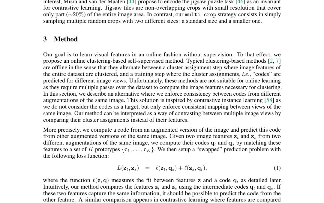
Figure 1: Contrastive instance learning (left) vs. SwAV (right). In contrastive learning methods applied to instance classification, the features from different transformations of the same images are compared directly to each other. In SwAV, we first obtain “codes” by assigning features to prototype vectors. We then solve a “swapped” prediction problem wherein the codes obtained from one data augmented view are predicted using the other view. Thus, SwAV does not directly compare image features. Prototype vectors are learned along with the ConvNet parameters by backpropragation.
| 对比实例学习 | 视图间交换分配(本文) |
图 1:对比实例学习(左)与 SwAV(右)。在应用于实例分类的对比学习方法中,来自同一图像不同变换的特征被直接相互比较。在 SwAV 中,我们先把特征分配到原型向量得到「码」,再求解「交换」预测问题:用一个数据增强视图预测从另一视图得到的码。因此 SwAV 不直接比较图像特征。原型向量与卷积网络参数一起通过反向传播学习。
3.1 Online clustering
3.1 在线聚类
Each image is transformed into an augmented view by applying a transformation sampled from the set of image transformations. The augmented view is mapped to a vector representation by applying a non-linear mapping to . The feature is then projected to the unit sphere, i.e., . We then compute a code from this feature by mapping to a set of trainable prototypes vectors, . We denote by the matrix whose columns are the . We now describe how to compute these codes and update the prototypes online.
每张图像 经从变换集合 采样的变换 得到增强视图 。增强视图经非线性映射 映到向量表示,再投影到单位球面,即 。随后把 映到一组 个可训练原型向量 得到编码 。记 为以 为列的矩阵。下面说明如何在线计算这些编码并更新原型。
Swapped prediction problem.
The loss function in Eq. (1) has two terms that setup the “swapped” prediction problem of predicting the code from the feature , and from . Each term represents the cross entropy loss between the code and the probability obtained by taking a softmax of the dot products of and all prototypes in , i.e.,
交换预测问题。
公式 (1) 的损失有两项,构成「交换」预测:从特征 预测编码 ,以及从 预测 。每项是编码与概率之间的交叉熵,概率由 与 中全部原型点积再 softmax 得到,即
where is a temperature parameter [58]. Taking this loss over all the images and pairs of data augmentations leads to the following loss function for the swapped prediction problem:
其中 为温度参数 [58]。在全部图像与成对数据增强上取该损失,得到交换预测问题的如下损失:
This loss function is jointly minimized with respect to the prototypes and the parameters of the image encoder used to produce the features .
该损失函数对原型 与用于产生特征 的图像编码器 的参数 联合最小化。
Computing codes online.
In order to make our method online, we compute the codes using only the image features within a batch. Intuitively, as the prototypes are used across different batches, SwAV clusters multiple instances to the prototypes. We compute codes using the prototypes such that all the examples in a batch are equally partitioned by the prototypes. This equipartition constraint ensures that the codes for different images in a batch are distinct, thus preventing the trivial solution where every image has the same code. Given feature vectors , we are interested in mapping them to the prototypes . We denote this mapping or codes by , and optimize to maximize the similarity between the features and the prototypes , i.e.,
在线计算编码。
为使方法在线,我们仅用 batch 内图像特征计算编码。直观上,由于原型 跨不同 batch 使用,SwAV 把多个实例聚类到原型上。我们用原型 计算编码,使 batch 中所有样本被原型均等划分。该等分约束确保 batch 内不同图像的编码彼此不同,从而防止每张图像得到同一编码的平凡解。给定 个特征向量 ,我们希望把它们映到原型 。记该映射或编码为 ,并优化 以最大化特征与原型的相似度,即
where is the entropy function, and is a parameter that controls the smoothness of the mapping. We observe that a strong entropy regularization (i.e. using a high ) generally leads to a trivial solution where all samples collapse into an unique representation and are all assigned uniformely to all prototypes. Hence, in practice we keep low. Asano et al. [2] enforce an equal partition by constraining the matrix to belong to the transportation polytope. They work on the full dataset, and we propose to adapt their solution to work on minibatches by restricting the transportation polytope to the minibatch:
其中 为熵函数,, 控制映射平滑度。我们观察到强熵正则(即高 )通常导致平凡解:所有样本塌缩到唯一表示,并被均匀分配到全部原型。因此实践中保持 较低。Asano 等人 [2] 通过约束矩阵 属于运输多面体来强制等分。他们在全数据集上工作;我们提议把解法改到小批量上,把运输多面体限制在小批量:
where denotes the vector of ones in dimension . These constraints enforce that on average each prototype is selected at least times in the batch.
其中 表示 维全 1 向量。这些约束强制平均每个原型在 batch 中至少被选 次。
Once a continuous solution to Prob. (3) is found, a discrete code can be obtained by using a rounding procedure [2]. Empirically, we found that discrete codes work well when computing codes in an offline manner on the full dataset as in Asano et al. [2]. However, in the online setting where we use only minibatches, using the discrete codes performs worse than using the continuous codes. An explanation is that the rounding needed to obtain discrete codes is a more aggressive optimization step than gradient updates. While it makes the model converge rapidly, it leads to a worse solution. We thus preserve the soft code instead of rounding it. These soft codes are the solution of Prob. (3) over the set and takes the form of a normalized exponential matrix [13]:
一旦找到问题 (3) 的连续解 ,可用舍入过程得到离散编码 [2]。经验上,像 Asano 等人 [2] 那样在全数据集上离线计算编码时,离散编码效果好。但在仅用小批量的在线设定中,离散编码不如连续编码。一种解释是:得到离散编码所需的舍入是比梯度更新更激进的优化步,虽使模型快速收敛,却通向更差解。因此我们保留软编码 而不舍入。这些软编码是问题 (3) 在集合 上的解,形式为归一化指数矩阵 [13]:
where and are renormalization vectors in and respectively. The renormalization vectors are computed using a small number of matrix multiplications using the iterative Sinkhorn-Knopp algorithm [13]. In practice, we observe that using only iterations is fast and sufficient to obtain good performance. Indeed, this algorithm can be efficiently implemented on GPU, and the alignment of K features to K codes takes ms in our experiments, see section 4.
其中 与 分别为 与 中的重归一化向量。重归一化向量用迭代 Sinkhorn-Knopp 算法 [13]、经少量矩阵乘法计算。实践中我们观察到仅用 次迭代就又快又够用。该算法可在 GPU 上高效实现;实验中把 K 特征对齐到 K 编码约需 ms,见第 4 节。
Working with small batches.
When the number of batch features is too small compared to the number of prototypes , it is impossible to equally partition the batch into the prototypes. Therefore, when working with small batches, we use features from the previous batches to augment the size of in Prob. (3). Then, we only use the codes of the batch features in our training loss. In practice, we store around K features, i.e., in the same range as the number of code vectors. This means that we only keep features from the last batches with a batch size of , while contrastive methods typically need to store the last K instances obtained from the last batches [24].
处理小 batch。
当 batch 特征数 相对原型数 过小时,无法把 batch 均等划分到 个原型。因此小 batch 时,我们用先前 batch 的特征扩充问题 (3) 中 的规模,训练损失中仍只用当前 batch 特征的编码。实践中约存 K 特征,即与编码向量数量同量级。这意味着 batch 为 时只需保留最近约 个 batch 的特征,而对比方法通常需存最近 个 batch 得到的约 K 实例 [24]。
| Method | Arch. | Param. | Top1 |
|---|---|---|---|
| Supervised | R50 | 24 | 76.5 |
| Colorization [65] | R50 | 24 | 39.6 |
| Jigsaw [46] | R50 | 24 | 45.7 |
| NPID [58] | R50 | 24 | 54.0 |
| BigBiGAN [15] | R50 | 24 | 56.6 |
| LA [68] | R50 | 24 | 58.8 |
| NPID++ [44] | R50 | 24 | 59.0 |
| MoCo [24] | R50 | 24 | 60.6 |
| SeLa [2] | R50 | 24 | 61.5 |
| PIRL [44] | R50 | 24 | 63.6 |
| CPC v2 [28] | R50 | 24 | 63.8 |
| PCL [37] | R50 | 24 | 65.9 |
| SimCLR [10] | R50 | 24 | 70.0 |
| MoCov2 [11] | R50 | 24 | 71.1 |
| SwAV | R50 | 24 | 75.3 |
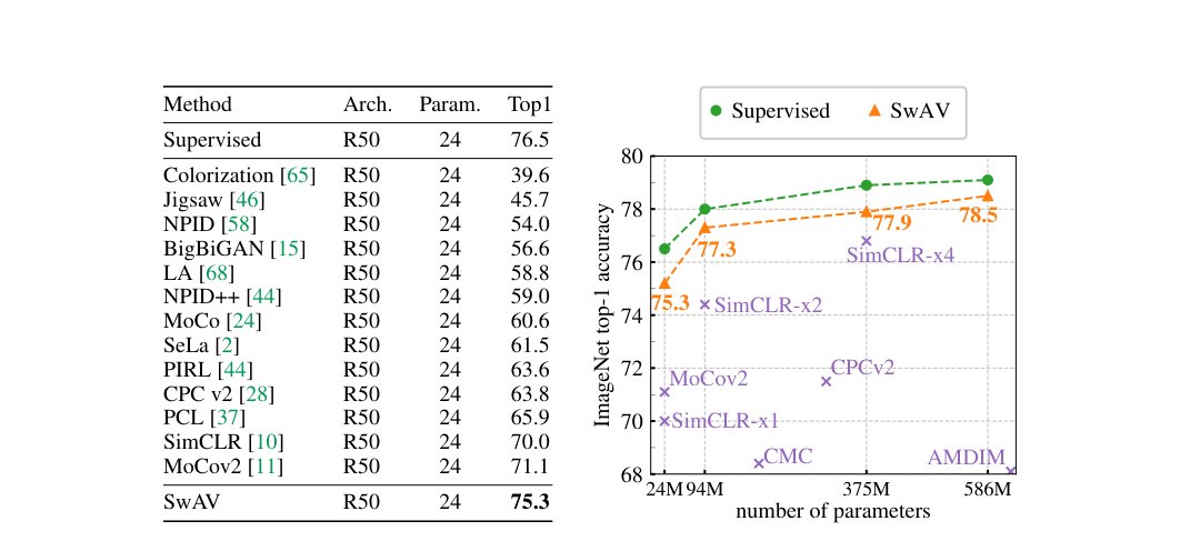
Figure 2: Linear classification on ImageNet. Top-1 accuracy for linear models trained on frozen features from different self-supervised methods. (left) Performance with a standard ResNet-50. (right) Performance as we multiply the width of a ResNet-50 by a factor , , and .
| 方法 | 架构 | 参数 | Top1 |
|---|---|---|---|
| Supervised | R50 | 24 | 76.5 |
| Colorization [65] | R50 | 24 | 39.6 |
| Jigsaw [46] | R50 | 24 | 45.7 |
| NPID [58] | R50 | 24 | 54.0 |
| BigBiGAN [15] | R50 | 24 | 56.6 |
| LA [68] | R50 | 24 | 58.8 |
| NPID++ [44] | R50 | 24 | 59.0 |
| MoCo [24] | R50 | 24 | 60.6 |
| SeLa [2] | R50 | 24 | 61.5 |
| PIRL [44] | R50 | 24 | 63.6 |
| CPC v2 [28] | R50 | 24 | 63.8 |
| PCL [37] | R50 | 24 | 65.9 |
| SimCLR [10] | R50 | 24 | 70.0 |
| MoCov2 [11] | R50 | 24 | 71.1 |
| SwAV | R50 | 24 | 75.3 |
图 2:ImageNet 上的线性分类。在不同自监督方法得到的冻结特征上训练线性模型的 top-1 准确率。(左) 标准 ResNet-50 上的表现。(右) 把 ResNet-50 宽度乘以 、、 时的表现。
3.2 Multi-crop: Augmenting views with smaller images
3.2 Multi-crop:用更小图像增强视图
As noted in prior works [10, 44], comparing random crops of an image plays a central role by capturing information in terms of relations between parts of a scene or an object. Unfortunately, increasing the number of crops or “views” quadratically increases the memory and compute requirements. We propose a multi-crop strategy where we use two standard resolution crops and sample additional low resolution crops that cover only small parts of the image. Using low resolution images ensures only a small increase in the compute cost. Specifically, we generalize the loss of Eq (1):
如先前工作 [10, 44] 所指出,比较图像的随机裁剪通过捕获场景或物体各部分之间的关系信息,扮演中心角色。不幸的是,增加裁剪或「视图」数量会使显存与算力需求二次增长。我们提出 multi-crop 策略:使用两个标准分辨率裁剪,再额外采样 个只覆盖图像小区域的低分辨率裁剪。使用低分辨率图像确保算力仅小幅增加。具体地,我们推广公式 (1) 的损失:
Note that we compute codes using only the full resolution crops. Indeed, computing codes for all crops increases the computational time and we observe in practice that it also alters the transfer performance of the resulting network. An explanation is that using only partial information (small crops cover only small area of images) degrades the assignment quality. Figure 3 shows that multi-crop improves the performance of several self-supervised methods and is a promising augmentation strategy.
注意我们只对全分辨率裁剪计算编码。确实,对所有裁剪算编码会增加计算时间,且实践中也观察到会损害所得网络的迁移表现。一种解释是:只用局部信息(小裁剪只覆盖小面积)会降低分配质量。图 3 显示 multi-crop 提升多种自监督方法的表现,是有前景的增强策略。
4 Main Results
4 主要结果
We analyze the features learned by SwAV by transfer learning on multiple datasets. We implement in SwAV the improvements used in SimCLR, i.e., LARS [64], cosine learning rate [40, 44] and the MLP projection head [10]. We provide the full details and hyperparameters for pretraining and transfer learning in the Appendix.
我们通过分析在多个数据集上的迁移学习来评估 SwAV 所学特征。SwAV 中实现了 SimCLR 所用改进,即 LARS [64]、余弦学习率 [40, 44] 与 MLP 投影头 [10]。预训练与迁移学习的完整细节与超参见附录。
4.1 Evaluating the unsupervised features on ImageNet
4.1 在 ImageNet 上评估无监督特征
We evaluate the features of a ResNet-50 [27] trained with SwAV on ImageNet by two experiments: linear classification on frozen features and semi-supervised learning by finetuning with few labels. When using frozen features (fig. 2 left), SwAV outperforms the state of the art by top-1 accuracy and is only below the performance of a fully supervised model. Note that we train SwAV during epochs with large batches (). We refer to fig. 3 for results with shorter trainings and to table 3 for experiments with small batches. On semi-supervised learning (table 1), SwAV outperforms other self-supervised methods and is on par with state-of-the-art semi-supervised models [51], despite the fact that SwAV is not specifically designed for semi-supervised learning.
我们用两个实验评估用 SwAV 在 ImageNet 上训练的 ResNet-50 [27] 特征:冻结特征上的线性分类,以及用少量标签微调的半监督学习。使用冻结特征时(图 2 左),SwAV 以 top-1 准确率超过此前最好结果,仅比全监督模型低 。注意我们用大批量()训练 SwAV 达 个 epoch。更短训练的结果见图 3,小 batch 实验见表 3。半监督学习上(表 1),SwAV 超过其他自监督方法,并与最好半监督模型 [51] 持平,尽管 SwAV 并非专为半监督设计。
| 1% labels | 10% labels | ||||||
|---|---|---|---|---|---|---|---|
| Method | Top-1 | Top-5 | Top-1 | Top-5 | |||
| Supervised | 25.4 | 48.4 | 56.4 | 80.4 | |||
| Methods using label-propagation | UDA [60] | - | - | 68.8 | 88.5 | ||
| FixMatch [51] | - | - | 71.5 | 89.1 | |||
| Methods using self-supervision only | PIRL [44] | 30.7 | 57.2 | 60.4 | 83.8 | ||
| PCL [37] | - | 75.6 | - | 86.2 | |||
| SimCLR [10] | 48.3 | 75.5 | 65.6 | 87.8 | |||
| SwAV | 53.9 | 78.5 | 70.2 | 89.9 |
Table 1: Semi-supervised learning on ImageNet with a ResNet-50. We finetune the model with and labels and report top-1 and top-5 accuracies. *:uses RandAugment [12].
| 1% labels | 10% labels | ||||||
|---|---|---|---|---|---|---|---|
| 方法 | Top-1 | Top-5 | Top-1 | Top-5 | |||
| Supervised | 25.4 | 48.4 | 56.4 | 80.4 | |||
| Methods using label-propagation | UDA [60] | - | - | 68.8 | 88.5 | ||
| FixMatch [51] | - | - | 71.5 | 89.1 | |||
| Methods using self-supervision only | PIRL [44] | 30.7 | 57.2 | 60.4 | 83.8 | ||
| PCL [37] | - | 75.6 | - | 86.2 | |||
| SimCLR [10] | 48.3 | 75.5 | 65.6 | 87.8 | |||
| SwAV | 53.9 | 78.5 | 70.2 | 89.9 |
表 1:用 ResNet-50 在 ImageNet 上半监督学习。用 与 标签微调模型,报告 top-1 与 top-5 准确率。:使用 RandAugment [12]。
Variants of ResNet-50. Figure 2 (right) shows the performance of multiple variants of ResNet-50 with different widths [35]. The performance of our model increases with the width of the model, and follows a similar trend to the one obtained with supervised learning. When compared with concurrent work like SimCLR, we see that SwAV reduces the difference with supervised models even further. Indeed, for large architectures, our method shrinks the gap with supervised training to .
ResNet-50 变体。图 2(右)展示不同宽度 ResNet-50 变体 [35] 的表现。我们的模型表现随宽度增加而提升,趋势与有监督学习相近。与 SimCLR 等同期工作相比,SwAV 进一步缩小与监督模型的差距。确实,对大架构,我们的方法把与监督训练的差距收至 。
| Linear Classification | Object Detection | ||||||
|---|---|---|---|---|---|---|---|
| Places205 | VOC07 | iNat18 | VOC07+12 | COCO | COCO | ||
| (Faster R-CNN R50-C4) | (Mask R-CNN R50-FPN) | (DETR) | |||||
| Supervised | 53.2 | 87.5 | 46.7 | 81.3 | 39.7 | 40.8 | |
| SwAV | 56.7 | 88.9 | 48.6 | 82.6 | 41.6 | 42.1 |
Table 2: Transfer learning on downstream tasks. Comparison between features from ResNet-50 trained on ImageNet with SwAV or supervised learning. We consider two settings. (1) Linear classification on top of frozen features. We report top-1 accuracy on all datasets except VOC07 where we report mAP. (2) Object detection with finetuned features on VOC07+12 trainval using Faster R-CNN [50] and on COCO [38] using Mask R-CNN [26] or DETR [6]. We report the most standard detection metrics for these datasets: on VOC07+12 and AP on COCO.
| Linear Classification | Object Detection | ||||||
|---|---|---|---|---|---|---|---|
| Places205 | VOC07 | iNat18 | VOC07+12 | COCO | COCO | ||
| (Faster R-CNN R50-C4) | (Mask R-CNN R50-FPN) | (DETR) | |||||
| Supervised | 53.2 | 87.5 | 46.7 | 81.3 | 39.7 | 40.8 | |
| SwAV | 56.7 | 88.9 | 48.6 | 82.6 | 41.6 | 42.1 |
表 2:下游任务上的迁移学习。比较用 SwAV 或有监督学习在 ImageNet 上训练的 ResNet-50 特征。考虑两种设定。(1) 冻结特征上的线性分类。除 VOC07 报 mAP 外,其余数据集报 top-1 准确率。(2) 在 VOC07+12 trainval 上用 Faster R-CNN [50]、在 COCO [38] 上用 Mask R-CNN [26] 或 DETR [6] 微调特征做目标检测。报告各数据集最常用检测指标:VOC07+12 上 ,COCO 上 AP。
4.2 Transferring unsupervised features to downstream tasks
4.2 把无监督特征迁移到下游任务
We test the generalization of ResNet-50 features trained with SwAV on ImageNet (without labels) by transferring to several downstream vision tasks. In table 2, we compare the performance of SwAV features with ImageNet supervised pretraining. First, we report the linear classification performance on the Places205 [67], VOC07 [17], and iNaturalist2018 [54] datasets. Our method outperforms supervised features on all three datasets. Note that SwAV is the first self-supervised method to surpass ImageNet supervised features on these datasets. Second, we report network finetuning on object detection on VOC07+12 using Faster R-CNN [50] with a R50-C4 backbone and on COCO [38] using Mask R-CNN [26] with a R50-FPN backbone and finally using DETR detector [6]. DETR is a recent object detection framework that reaches competitive performance with Faster R-CNN while being conceptually simpler and trainable end-to-end. Interestingly, unlike Faster R-CNN [50], using a pretrained backbone for DETR is crucial to obtain good results compared to training from scratch [6]. In table 2, we show that SwAV outperforms the supervised pretrained model on both VOC07+12 and COCO datasets. Note that this is line with previous works that also show that self-supervision can outperform supervised pretraining on object detection [44, 24, 19]. We report more detection evaluation metrics and results from other self-supervised methods in the Appendix. Overall, our SwAV ResNet-50 model surpasses supervised ImageNet pretraining on all the considered transfer tasks and datasets. We have released this model so other researchers might also benefit by replacing the ImageNet supervised network with our model.
我们通过迁移到若干下游视觉任务,检验用 SwAV 在 ImageNet(无标签)上训练的 ResNet-50 特征的泛化。表 2 比较 SwAV 特征与 ImageNet 有监督预训练。首先,我们报告 Places205 [67]、VOC07 [17] 与 iNaturalist2018 [54] 上的线性分类表现。我们的方法在三个数据集上都超过有监督特征。注意 SwAV 是首个在这些数据集上超过 ImageNet 有监督特征的自监督方法。其次,我们报告在 VOC07+12 上用 Faster R-CNN [50](R50-C4 骨干)微调做目标检测,以及在 COCO [38] 上用 Mask R-CNN [26](R50-FPN)与 DETR 检测器 [6] 的结果。DETR 是近期目标检测框架,在概念更简单、可端到端训练的同时达到与 Faster R-CNN 有竞争力的表现。有趣的是,与 Faster R-CNN [50] 不同,对 DETR 使用预训练骨干对取得相对从头训练的好结果至关重要 [6]。表 2 显示 SwAV 在 VOC07+12 与 COCO 上都超过有监督预训练模型。这与先前也显示自监督可在目标检测上超过有监督预训练的工作一致 [44, 24, 19]。更多检测评估指标及其他自监督方法结果见附录。总体而言,我们的 SwAV ResNet-50 模型在全部考虑的迁移任务与数据集上超过有监督 ImageNet 预训练。我们已发布该模型,其他研究者也可用它替换 ImageNet 监督网络。
4.3 Training with small batches
4.3 小 batch 训练
We train SwAV with small batches of images on GPUs and compare with MoCov2 and SimCLR trained in the same setup. In table 3, we see that SwAV maintains state-of-the-art performance even when trained in the small batch setting. Note that SwAV only stores a queue of features. In comparison, to obtain good performance, MoCov2 needs to store features while keeping an additional momentum encoder network. When SwAV is trained using crops, SwAV has a running time higher than SimCLR with crops and is around slower than MoCov2 due to the additional back-propagation [11]. Hence, one epoch of MoCov2 or SimCLR is faster in wall clock time than one of SwAV, but these methods need more epochs for good downstream performance. Indeed, as shown in table 3, SwAV learns much faster and reaches higher performance in fewer epochs: after epochs ( hours) while MoCov2 needs epochs to achieve . Increasing the resolution and the number of epochs, SwAV reaches with a small batch size, a small number of stored features and no momentum encoder. Finally, note that SwAV could be combined with a momentum mechanism and a large queue [24]; we leave these explorations to future work.
我们在 张 GPU 上用 图像的小 batch 训练 SwAV,并与同设定下的 MoCov2 与 SimCLR 比较。表 3 显示即便小 batch,SwAV 仍保持最好表现。注意 SwAV 只存约 个特征的队列。相比之下,MoCov2 为取得好表现需存 个特征,并额外保留动量编码器网络。当 SwAV 使用 裁剪时,运行时间比用 裁剪的 SimCLR 高 ,因额外反向传播约比 MoCov2 慢 [11]。因此 MoCov2 或 SimCLR 的单 epoch 墙钟时间更快,但这些方法需要更多 epoch 才能有好的下游表现。如表 3 所示,SwAV 学得快得多,用 更少 epoch 达到更高表现: 个 epoch( 小时)后 ,而 MoCov2 需 个 epoch 才到 。提高分辨率与 epoch 数后,SwAV 在小 batch、少量存特征且无动量编码器时达到 。最后注意 SwAV 可与动量机制及大队列结合 [24];这些探索留待未来工作。
| Method | Mom. Encoder | Stored Features | multi-crop | epoch | batch | Top-1 |
|---|---|---|---|---|---|---|
| SimCLR | ||||||
| MoCov2 | ✓ | |||||
| MoCov2 | ✓ | |||||
| SwAV | + | |||||
| SwAV | + | |||||
| SwAV | + |
Table 3: Training in small batch setting. Top-1 accuracy on ImageNet with a linear classifier trained on top of frozen features from a ResNet-50. All methods are trained with a batch size of . We also report the number of stored features, the type of cropping used and the number of epochs.
| 方法 | 动量编码器 | 存特征数 | multi-crop | epoch | batch | Top-1 |
|---|---|---|---|---|---|---|
| SimCLR | ||||||
| MoCov2 | ✓ | |||||
| MoCov2 | ✓ | |||||
| SwAV | + | |||||
| SwAV | + | |||||
| SwAV | + |
表 3:小 batch 设定下的训练。在 ResNet-50 冻结特征上训练线性分类器的 ImageNet top-1 准确率。全部方法 batch 为 。我们也报告存特征数、所用裁剪类型与 epoch 数。
5 Ablation Study
5 消融研究
5.1 Clustering-based self-supervised learning
5.1 基于聚类的自监督学习
Improving prior clustering-based approaches.
In this section, we re-implement and improve previously published clustering-based models in order to assess if they can compete with recent contrastive methods such as SimCLR. In particular, we consider two clustering-based models: DeepCluster-v2 and SeLa-v2, which are obtained by applying various training improvements introduced in other self-supervised learning papers to DeepCluster [7] and SeLa [2]. Among these improvements are the use of stronger data augmentation [10], MLP projection head [10], cosine learning rate schedule [44], temperature parameter [58], memory bank [58], multi-clustering [2], etc. Full implementation details can be found in the Appendix. Besides, we also improve DeepCluster model by introducing explicit comparisons to k-means centroids, which increase stability and performance. Indeed, a main issue in DeepCluster is that there is no correspondance between two consecutive cluster assignments. Hence, the final classification layer learned for an assignment becomes irrelevant for the following one and thus needs to be re-initialized from scratch at each epoch. This considerably disrupts the convnet training. In DeepCluster-v2, instead of learning a classification layer predicting the cluster assignments, we perform explicit comparison between features and centroids.
改进先前基于聚类的方法。
本节重实现并改进先前发表的基于聚类模型,以评估它们能否与 SimCLR 等近期对比方法竞争。我们特别考虑两个基于聚类的模型:DeepCluster-v2 与 SeLa-v2,它们是把其他自监督论文中的多种训练改进应用到 DeepCluster [7] 与 SeLa [2] 上得到的。这些改进包括更强数据增强 [10]、MLP 投影头 [10]、余弦学习率调度 [44]、温度参数 [58]、记忆库 [58]、多聚类 [2] 等。完整实现细节见附录。此外,我们还通过引入与 k-means 中心的显式比较来改进 DeepCluster 模型,以提升稳定性与表现。DeepCluster 的一个主要问题是连续两次聚类分配之间没有对应关系。因此,为某次分配学到的最终分类层对下一次分配变得无关,需要每个 epoch 从头重新初始化,这会严重干扰卷积网络训练。在 DeepCluster-v2 中,我们不再学习预测聚类分配的分类层,而是在特征与中心之间做显式比较。
| Top-1 | |||
|---|---|---|---|
| Method | 2x224 | 2x160+4x96 | |
| Supervised | |||
| Contrastive-instance approaches | |||
| SimCLR | |||
| Clustering-based approaches | |||
| SeLa-v2 | |||
| DeepCluster-v2 | |||
| SwAV |
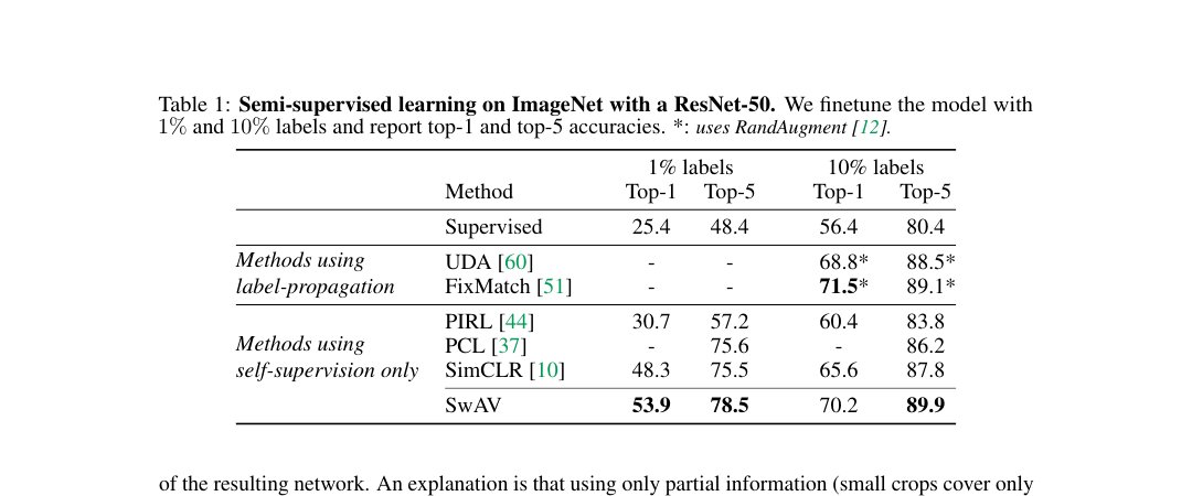
Figure 3: Top-1 accuracy on ImageNet with a linear classifier trained on top of frozen features from a ResNet-50. (left) Comparison between clustering-based and contrastive instance methods and impact of multi-crop. Self-supervised methods are trained for epochs and supervised models for epochs. (right) Performance as a function of epochs. We compare SwAV models trained with different number of epochs and report their running time based on our implementation.
| Top-1 | |||
|---|---|---|---|
| 方法 | 2x224 | 2x160+4x96 | |
| Supervised | |||
| Contrastive-instance approaches | |||
| SimCLR | |||
| Clustering-based approaches | |||
| SeLa-v2 | |||
| DeepCluster-v2 | |||
| SwAV |
图 3:在 ResNet-50 冻结特征上训练线性分类器的 ImageNet top-1 准确率。(左) 基于聚类与对比实例方法的比较以及 multi-crop 的影响。自监督方法训 个 epoch,有监督模型训 个 epoch。(右) 表现随 epoch 数变化。我们比较不同 epoch 数训练的 SwAV 模型,并按我们的实现报告运行时间。
Comparing clustering with contrastive instance learning.
In fig. 3 (left), we make a best effort fair comparison between clustering-based and contrastive instance (SimCLR) methods by implementating these methods with the same data augmentation, number of epochs, batch-sizes, etc. In this setting, we observe that SwAV and DeepCluster-v2 outperform SimCLR by without multi-crop and by with multi-crop. This suggests the learning potential of clustering-based methods over instance classification.
比较聚类与对比实例学习。
在图 3(左),我们尽量公平地比较基于聚类的方法与对比实例(SimCLR)方法:用相同数据增强、epoch 数、batch 大小等实现。该设定下,无 multi-crop 时 SwAV 与 DeepCluster-v2 比 SimCLR 高 ,有 multi-crop 时高 。这表明基于聚类的方法相对实例分类具有学习潜力。
Advantage of SwAV compared to DeepCluster-v2.
In fig. 3 (left), we observe that SwAV performs on par with DeepCluster-v2. In addition, we train DeepCluster-v2 in SwAV best setting (800 epochs - 8 crops) and obtain top-1 accuracy on ImageNet (versus for SwAV). However, unlike SwAV, DeepCluster-v2 is not online which makes it impractical for extremely large datasets (section 5.4). For billion scale trainings for example, a single pass on the dataset is usually performed [24]. DeepCluster-v2 cannot be trained for only one epoch since it works by performing several passes on the dataset to regularly update centroids and cluster assignments for each image.
相对 DeepCluster-v2,SwAV 的优势。
图 3(左)显示 SwAV 与 DeepCluster-v2 表现相当。此外,我们在 SwAV 最佳设定(800 epoch、8 裁剪)下训练 DeepCluster-v2,在 ImageNet 上得到 top-1(SwAV 为 )。但与 SwAV 不同,DeepCluster-v2 非在线,难以用于极大数据集(第 5.4 节)。例如十亿级训练通常只对数据集做单次遍历 [24]。DeepCluster-v2 无法只训一个 epoch,因为它靠对数据集多轮遍历来定期更新中心与每张图像的聚类分配。
As a matter of fact, DeepCluster-v2 can be interpreted as a special case of our proposed swapping mechanism: swapping is done across epochs rather than within a batch. Given a crop of an image DeepCluster-v2 predicts the assignment of another crop, which was obtained at the previous epoch. SwAV swaps assignments directly at the batch level and can thus work online.
事实上,DeepCluster-v2 可解读为我们所提交换机制的特例:交换跨 epoch 进行,而非在 batch 内。给定图像的一个裁剪,DeepCluster-v2 预测上一 epoch 得到的另一裁剪的分配。SwAV 直接在 batch 级交换分配,因而可在线工作。
5.2 Applying the multi-crop strategy to different methods
5.2 把 multi-crop 策略用于不同方法
In fig. 3 (left), we report the impact of applying our multi-crop strategy on the performance of a selection of other methods. Details of how we apply multi-crop to SimCLR loss can be found in the Appendix. We see that the multi-crop strategy consistently improves the performance for all the considered methods by a significant margin of top-1 accuracy. Interestingly, multi-crop seems to benefit more clustering-based methods than contrastive methods. We note that multi-crop does not improve the supervised model.
图 3(左)报告把我们的 multi-crop 策略用于若干其他方法时的影响。如何把 multi-crop 用于 SimCLR 损失的细节见附录。可见 multi-crop 策略对全部考虑的方法都有显著提升,约 top-1 准确率。有趣的是,multi-crop 对基于聚类的方法似乎比对对比方法更有益。我们注意到 multi-crop 并不提升有监督模型。
5.3 Impact of longer training
5.3 更长训练的影响
In fig. 3 (right), we show the impact of the number of training epochs on performance for SwAV with multi-crop. We train separate models for , , and epochs and report the top-1 accuracy on ImageNet using the linear classification evaluation. We train each ResNet-50 on V100 16GB GPUs and a batch size of . While SwAV benefits from longer training, it already achieves strong performance after epochs, i.e., in 6h15.
图 3(右)展示带 multi-crop 的 SwAV 上训练 epoch 数对表现的影响。我们分别训 、、 与 个 epoch 的独立模型,并用线性分类评估报告 ImageNet top-1。每个 ResNet-50 在 张 V100 16GB GPU 上、batch 训练。虽 SwAV 受益于更长训练,但 个 epoch 后已很强,即 6 小时 15 分内达到 。
5.4 Unsupervised pretraining on a large uncurated dataset
5.4 在大型未策展数据集上无监督预训练
We evaluate SwAV on random, uncurated images that have different properties from ImageNet which allows us to test if our online clustering scheme and multi-crop augmentation work out of the box. In particular, we pretrain SwAV on an uncurated dataset of 1 billion random public non-EU images from Instagram. We test if SwAV can serve as a pretraining method for supervised learning. In fig. 4 (left), we measure the performance of ResNet-50 models when transferring to ImageNet with frozen or finetuned features. We report the results from He et al. [24] but note that their setting is different. They use a curated set of Instagram images, filtered by hashtags similar to ImageNet labels [41]. We compare SwAV with a randomly initialized network and with a network pretrained on the same data using SimCLR. We observe that SwAV maintains a similar gain of over SimCLR as when pretrained on ImageNet (fig. 2), showing that our improvements do not depend on the data distribution. We also see that pretraining with SwAV on random images significantly improves over training from scratch on ImageNet () [8, 24]. This result is in line with Caron et al. [8] and He et al. [24]. In fig. 4 (right), we explore the limits of pretraining as we increase the model capacity. We consider the variants of the ResNeXt architecture [61] as in Mahajan et al. [41]. We compare SwAV with supervised models trained from scratch on ImageNet. For all models, SwAV outperforms training from scratch by a significant margin showing that it can take advantage of the increased model capacity. For reference, we also include the results from Mahajan et al. [41] obtained with a weakly-supervised model pretrained by predicting hashtags filtered to be similar to ImageNet classes. Interestingly, SwAV performance is strong when compared to this topline despite not using any form of supervision or filtering of the data.
我们在随机、未策展、与 ImageNet 性质不同的图像上评估 SwAV,以检验在线聚类方案与 multi-crop 增强能否开箱即用。具体地,我们在来自 Instagram 的 10 亿张随机公开非欧盟图像的未策展数据集上预训练 SwAV,并测试 SwAV 能否作为有监督学习的预训练方法。图 4(左)测量把 ResNet-50 以冻结或微调特征迁移到 ImageNet 时的表现。我们报告 He 等人 [24] 的结果,但注意其设定不同:他们使用按与 ImageNet 标签相似的话题标签过滤的策展 Instagram 图像集 [41]。我们把 SwAV 与随机初始化网络、以及用 SimCLR 在相同数据上预训练的网络比较。观察到 SwAV 相对 SimCLR 保持与在 ImageNet 上预训练时类似的约 收益(图 2),说明我们的改进不依赖数据分布。我们也看到在随机图像上用 SwAV 预训练显著优于在 ImageNet 上从头训练() [8, 24]。这与 Caron 等人 [8] 与 He 等人 [24] 一致。图 4(右)探索增大模型容量时预训练的上限。我们按 Mahajan 等人 [41] 考虑 ResNeXt 架构变体 [61],并把 SwAV 与在 ImageNet 上从头训练的有监督模型比较。对全部模型,SwAV 都以显著幅度超过从头训练,说明它能利用增大的模型容量。作为参考,我们也纳入 Mahajan 等人 [41] 用弱监督模型、通过预测过滤为与 ImageNet 类相似的话题标签得到的结果。有趣的是,尽管不使用任何形式的监督或数据过滤,SwAV 相对该上沿仍表现强劲。
| Method | Frozen | Finetuned |
|---|---|---|
| Random | 15.0 | 76.5 |
| MoCo | - | 77.3 |
| SimCLR | 60.4 | 77.2 |
| SwAV | 66.5 | 77.8 |
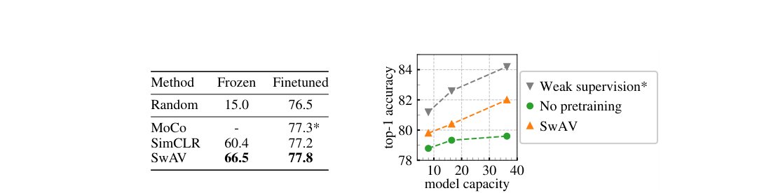
Figure 4: Pretraining on uncurated data. Top-1 accuracy on ImageNet for pretrained models on an uncurated set of 1B random Instagram images. (left) We compare ResNet-50 pretrained with either SimCLR or SwAV on two downstream tasks: linear classification on frozen features or finetuned features. (right) Performance of finetuned models as we increase the capacity of a ResNext following [41]. The capacity is provided in billions of Mult-Add operations. *: pretrained on a curated set of B Instagram images filtered with k hashtags similar to ImageNet classes.
| 方法 | 冻结 | 微调 |
|---|---|---|
| Random | 15.0 | 76.5 |
| MoCo | - | 77.3 |
| SimCLR | 60.4 | 77.2 |
| SwAV | 66.5 | 77.8 |
图 4:在未策展数据上预训练。在 10 亿张随机 Instagram 图像的未策展集上预训练模型后,ImageNet top-1 准确率。(左) 比较用 SimCLR 或 SwAV 预训练的 ResNet-50 在两个下游任务上:冻结特征线性分类或微调特征。(右) 按 [41] 增大 ResNeXt 容量时微调模型的表现。容量以十亿次乘加运算计。*:在用与 ImageNet 类相似的 k 话题标签过滤的 B 策展 Instagram 图像上预训练。
6 Discussion
6 讨论
Self-supervised learning is rapidly progressing compared to supervised learning, even surpassing it on transfer learning, even though the current experimental settings are designed for supervised learning. In particular, architectures have been designed for supervised tasks, and it is not clear if the same models would emerge from exploring architectures with no supervision. Several recent works have shown that exploring architectures with search [39] or pruning [9] is possible without supervision, and we plan to evaluate the ability of our method to guide model explorations.
自监督学习相对有监督学习进展迅速,甚至在迁移学习上超过后者,尽管当前实验设定是为有监督学习设计的。尤其是,架构为有监督任务而设计,尚不清楚在无监督下探索架构是否会涌现相同模型。若干近期工作表明,无需监督即可用搜索 [39] 或剪枝 [9] 探索架构;我们计划评估方法引导模型探索的能力。
Acknowledgement.
We thank Nicolas Carion, Kaiming He, Herve Jegou, Benjamin Lefaudeux, Thomas Lucas, Francisco Massa, Sergey Zagoruyko, and the rest of Thoth and FAIR teams for their help and fruitful discussions. Julien Mairal was funded by the ERC grant number 714381 (SOLARIS project) and by ANR 3IA MIAI@Grenoble Alpes (ANR-19-P3IA-0003).
致谢。
我们感谢 Nicolas Carion、Kaiming He、Herve Jegou、Benjamin Lefaudeux、Thomas Lucas、Francisco Massa、Sergey Zagoruyko 以及 Thoth 与 FAIR 其余团队的帮助与富有成果的讨论。Julien Mairal 由 ERC 资助号 714381(SOLARIS 项目)以及 ANR 3IA MIAI@Grenoble Alpes(ANR-19-P3IA-0003)资助。
References
参考文献
[1] Agrawal, P., Carreira, J., Malik, J.: Learning to see by moving. In: Proceedings of the International Conference on Computer Vision (ICCV) (2015)
[2] Asano, Y.M., Rupprecht, C., Vedaldi, A.: Self-labelling via simultaneous clustering and representation learning. International Conference on Learning Representations (ICLR) (2020)
[3] Bachman, P., Hjelm, R.D., Buchwalter, W.: Learning representations by maximizing mutual information across views. In: Advances in Neural Information Processing Systems (NeurIPS) (2019)
[4] Bautista, M.A., Sanakoyeu, A., Tikhoncheva, E., Ommer, B.: Cliquecnn: Deep unsupervised exemplar learning. In: Advances in Neural Information Processing Systems (NeurIPS) (2016)
[5] Bojanowski, P., Joulin, A.: Unsupervised learning by predicting noise. In: Proceedings of the International Conference on Machine Learning (ICML) (2017)
[6] Carion, N., Massa, F., Synnaeve, G., Usunier, N., Kirillov, A., Zagoruyko, S.: End-to-end object detection with transformers. arXiv preprint arXiv:2005.12872 (2020)
[7] Caron, M., Bojanowski, P., Joulin, A., Douze, M.: Deep clustering for unsupervised learning of visual features. In: Proceedings of the European Conference on Computer Vision (ECCV) (2018)
[8] Caron, M., Bojanowski, P., Mairal, J., Joulin, A.: Unsupervised pre-training of image features on non-curated data. In: Proceedings of the International Conference on Computer Vision (ICCV) (2019)
[9] Caron, M., Morcos, A., Bojanowski, P., Mairal, J., Joulin, A.: Pruning convolutional neural networks with self-supervision. arXiv preprint arXiv:2001.03554 (2020)
[10] Chen, T., Kornblith, S., Norouzi, M., Hinton, G.: A simple framework for contrastive learning of visual representations. arXiv preprint arXiv:2002.05709 (2020)
[11] Chen, X., Fan, H., Girshick, R., He, K.: Improved baselines with momentum contrastive learning. arXiv preprint arXiv:2003.04297 (2020)
[12] Cubuk, E.D., Zoph, B., Shlens, J., Le, Q.V.: Randaugment: Practical data augmentation with no separate search. arXiv preprint arXiv:1909.13719 (2019)
[13] Cuturi, M.: Sinkhorn distances: Lightspeed computation of optimal transport. In: Advances in Neural Information Processing Systems (NeurIPS) (2013)
[14] Doersch, C., Gupta, A., Efros, A.A.: Unsupervised visual representation learning by context prediction. In: Proceedings of the International Conference on Computer Vision (ICCV) (2015)
[15] Donahue, J., Simonyan, K.: Large scale adversarial representation learning. In: Advances in Neural Information Processing Systems (NeurIPS) (2019)
[16] Dosovitskiy, A., Fischer, P., Springenberg, J.T., Riedmiller, M., Brox, T.: Discriminative unsupervised feature learning with exemplar convolutional neural networks. IEEE transactions on pattern analysis and machine intelligence 38 (9), 1734–1747 (2016)
[17] Everingham, M., Van Gool, L., Williams, C.K., Winn, J., Zisserman, A.: The pascal visual object classes (voc) challenge. International journal of computer vision 88 (2), 303–338 (2010)
[18] Fan, R.E., Chang, K.W., Hsieh, C.J., Wang, X.R., Lin, C.J.: Liblinear: A library for large linear classification. Journal of machine learning research (2008)
[19] Gidaris, S., Bursuc, A., Komodakis, N., Pérez, P., Cord, M.: Learning representations by predicting bags of visual words. arXiv preprint arXiv:2002.12247 (2020)
[20] Gidaris, S., Singh, P., Komodakis, N.: Unsupervised representation learning by predicting image rotations. In: International Conference on Learning Representations (ICLR) (2018)
[21] Goyal, P., Dollár, P., Girshick, R., Noordhuis, P., Wesolowski, L., Kyrola, A., Tulloch, A., Jia, Y., He, K.: Accurate, large minibatch sgd: Training imagenet in 1 hour. arXiv preprint arXiv:1706.02677 (2017)
[22] Gutmann, M., Hyvärinen, A.: Noise-contrastive estimation: A new estimation principle for unnormalized statistical models. In: Proceedings of the Thirteenth International Conference on Artificial Intelligence and Statistics (2010)
[23] Hadsell, R., Chopra, S., LeCun, Y.: Dimensionality reduction by learning an invariant mapping. In: Proceedings of the Conference on Computer Vision and Pattern Recognition (CVPR) (2006)
[24] He, K., Fan, H., Wu, Y., Xie, S., Girshick, R.: Momentum contrast for unsupervised visual representation learning. arXiv preprint arXiv:1911.05722 (2019)
[25] He, K., Girshick, R., Dollár, P.: Rethinking imagenet pre-training. In: Proceedings of the International Conference on Computer Vision (ICCV) (2019)
[26] He, K., Gkioxari, G., Dollár, P., Girshick, R.: Mask r-cnn. In: Proceedings of the International Conference on Computer Vision (ICCV) (2017)
[27] He, K., Zhang, X., Ren, S., Sun, J.: Deep residual learning for image recognition. In: Proceedings of the Conference on Computer Vision and Pattern Recognition (CVPR) (2016)
[28] Hénaff, O.J., Razavi, A., Doersch, C., Eslami, S., Oord, A.v.d.: Data-efficient image recognition with contrastive predictive coding. arXiv preprint arXiv:1905.09272 (2019)
[29] Hjelm, R.D., Fedorov, A., Lavoie-Marchildon, S., Grewal, K., Bachman, P., Trischler, A., Bengio, Y.: Learning deep representations by mutual information estimation and maximization. International Conference on Learning Representations (ICLR) (2019)
[30] Huang, J., Dong, Q., Gong, S.: Unsupervised deep learning by neighbourhood discovery. In: Proceedings of the International Conference on Machine Learning (ICML) (2019)
[31] Jenni, S., Favaro, P.: Self-supervised feature learning by learning to spot artifacts. In: Proceedings of the Conference on Computer Vision and Pattern Recognition (CVPR) (2018)
[32] Jing, L., Tian, Y.: Self-supervised visual feature learning with deep neural networks: A survey. arXiv preprint arXiv:1902.06162 (2019)
[33] Khosla, P., Teterwak, P., Wang, C., Sarna, A., Tian, Y., Isola, P., Maschinot, A., Liu, C., Krishnan, D.: Supervised contrastive learning. arXiv preprint arXiv:2004.11362 (2020)
[34] Kim, D., Cho, D., Yoo, D., Kweon, I.S.: Learning image representations by completing damaged jigsaw puzzles. In: Winter Conference on Applications of Computer Vision (WACV) (2018)
[35] Kolesnikov, A., Zhai, X., Beyer, L.: Revisiting self-supervised visual representation learning. In: Proceedings of the Conference on Computer Vision and Pattern Recognition (CVPR) (2019)
[36] Larsson, G., Maire, M., Shakhnarovich, G.: Learning representations for automatic colorization. In: Proceedings of the European Conference on Computer Vision (ECCV) (2016)
[37] Li, J., Zhou, P., Xiong, C., Socher, R., Hoi, S.C.: Prototypical contrastive learning of unsupervised representations. arXiv preprint arXiv:2005.04966 (2020)
[38] Lin, T.Y., Maire, M., Belongie, S., Hays, J., Perona, P., Ramanan, D., Dollár, P., Zitnick, C.L.: Microsoft coco: Common objects in context. In: Proceedings of the European Conference on Computer Vision (ECCV) (2014)
[39] Liu, C., Dollár, P., He, K., Girshick, R., Yuille, A., Xie, S.: Are labels necessary for neural architecture search? arXiv preprint arXiv:2003.12056 (2020)
[40] Loshchilov, I., Hutter, F.: Sgdr: Stochastic gradient descent with warm restarts. arXiv preprint arXiv:1608.03983 (2016)
[41] Mahajan, D., Girshick, R., Ramanathan, V., He, K., Paluri, M., Li, Y., Bharambe, A., van der Maaten, L.: Exploring the limits of weakly supervised pretraining. In: Proceedings of the European Conference on Computer Vision (ECCV) (2018)
[42] Mahendran, A., Thewlis, J., Vedaldi, A.: Cross pixel optical flow similarity for self-supervised learning. arXiv preprint arXiv:1807.05636 (2018)
[43] Micikevicius, P., Narang, S., Alben, J., Diamos, G., Elsen, E., Garcia, D., Ginsburg, B., Houston, M., Kuchaiev, O., Venkatesh, G., et al.: Mixed precision training. arXiv preprint arXiv:1710.03740 (2017)
[44] Misra, I., van der Maaten, L.: Self-supervised learning of pretext-invariant representations. arXiv preprint arXiv:1912.01991 (2019)
[45] Misra, I., Zitnick, C.L., Hebert, M.: Shuffle and learn: unsupervised learning using temporal order verification. In: Proceedings of the European Conference on Computer Vision (ECCV) (2016)
[46] Noroozi, M., Favaro, P.: Unsupervised learning of visual representations by solving jigsaw puzzles. In: Proceedings of the European Conference on Computer Vision (ECCV) (2016)
[47] Oord, A.v.d., Li, Y., Vinyals, O.: Representation learning with contrastive predictive coding. arXiv preprint arXiv:1807.03748 (2018)
[48] Pathak, D., Girshick, R., Dollár, P., Darrell, T., Hariharan, B.: Learning features by watching objects move. In: Proceedings of the Conference on Computer Vision and Pattern Recognition (CVPR) (2017)
[49] Pathak, D., Krahenbuhl, P., Donahue, J., Darrell, T., Efros, A.A.: Context encoders: Feature learning by inpainting. In: Proceedings of the Conference on Computer Vision and Pattern Recognition (CVPR) (2016)
[50] Ren, S., He, K., Girshick, R., Sun, J.: Faster r-cnn: Towards real-time object detection with region proposal networks. In: Advances in Neural Information Processing Systems (NeurIPS) (2015)
[51] Sohn, K., Berthelot, D., Li, C.L., Zhang, Z., Carlini, N., Cubuk, E.D., Kurakin, A., Zhang, H., Raffel, C.: Fixmatch: Simplifying semi-supervised learning with consistency and confidence. arXiv preprint arXiv:2001.07685 (2020)
[52] Tian, Y., Krishnan, D., Isola, P.: Contrastive multiview coding. arXiv preprint arXiv:1906.05849 (2019)
[53] Touvron, H., Vedaldi, A., Douze, M., Jégou, H.: Fixing the train-test resolution discrepancy. In: Advances in Neural Information Processing Systems (NeurIPS) (2019)
[54] Van Horn, G., Mac Aodha, O., Song, Y., Cui, Y., Sun, C., Shepard, A., Adam, H., Perona, P., Belongie, S.: The inaturalist species classification and detection dataset. In: Proceedings of the Conference on Computer Vision and Pattern Recognition (CVPR) (2018)
[55] Wang, X., Gupta, A.: Unsupervised learning of visual representations using videos. In: Proceedings of the International Conference on Computer Vision (ICCV) (2015)
[56] Wang, X., He, K., Gupta, A.: Transitive invariance for self-supervised visual representation learning. In: Proceedings of the International Conference on Computer Vision (ICCV) (2017)
[57] Wu, Y., Kirillov, A., Massa, F., Lo, W.Y., Girshick, R.: Detectron2. https://github.com/facebookresearch/detectron2 (2019)
[58] Wu, Z., Xiong, Y., Yu, S.X., Lin, D.: Unsupervised feature learning via non-parametric instance discrimination. In: Proceedings of the Conference on Computer Vision and Pattern Recognition (CVPR) (2018)
[59] Xie, J., Girshick, R., Farhadi, A.: Unsupervised deep embedding for clustering analysis. In: Proceedings of the International Conference on Machine Learning (ICML) (2016)
[60] Xie, Q., Dai, Z.D., Hovy, E., Luong, M.T., Le, Q.V.: Unsupervised data augmentation for consistency training. arXiv preprint arXiv:1904.12848 (2020)
[61] Xie, S., Girshick, R., Dollár, P., Tu, Z., He, K.: Aggregated residual transformations for deep neural networks. In: Proceedings of the Conference on Computer Vision and Pattern Recognition (CVPR) (2017)
[62] Yan, X., Misra, Ishan, I., Gupta, A., Ghadiyaram, D., Mahajan, D.: ClusterFit: Improving generalization of visual representations. In: Proceedings of the Conference on Computer Vision and Pattern Recognition (CVPR) (2020)
[63] Yang, J., Parikh, D., Batra, D.: Joint unsupervised learning of deep representations and image clusters. In: Proceedings of the Conference on Computer Vision and Pattern Recognition (CVPR) (2016)
[64] You, Y., Gitman, I., Ginsburg, B.: Large batch training of convolutional networks. arXiv preprint arXiv:1708.03888 (2017)
[65] Zhang, R., Isola, P., Efros, A.A.: Colorful image colorization. In: Proceedings of the European Conference on Computer Vision (ECCV) (2016)
[66] Zhang, R., Isola, P., Efros, A.A.: Split-brain autoencoders: Unsupervised learning by cross-channel prediction. In: Proceedings of the Conference on Computer Vision and Pattern Recognition (CVPR) (2017)
[67] Zhou, B., Lapedriza, A., Xiao, J., Torralba, A., Oliva, A.: Learning deep features for scene recognition using places database. In: Advances in Neural Information Processing Systems (NeurIPS) (2014)
[68] Zhuang, C., Zhai, A.L., Yamins, D.: Local aggregation for unsupervised learning of visual embeddings. In: Proceedings of the International Conference on Computer Vision (ICCV) (2019)
A Implementation Details
A 实现细节
In this section, we provide the details and hyperparameters for SwAV pretraining and transfer learning. Our code is publicly available at https://github.com/facebookresearch/swav.
本节给出 SwAV 预训练与迁移学习的细节与超参数。代码公开于 https://github.com/facebookresearch/swav。
A.1 Implementation details of SwAV training
First, we provide a pseudo-code for SwAV training loop using two crops in Pytorch style: # C: prototypes (DxK) # model: convnet + projection head # temp: temperature for x in loader: # load a batch x with B samples x_t = t(x) # t is a random augmentation x_s = s(x) # s is a another random augmentation z = model(cat(x_t, x_s)) # embeddings: 2BxD scores = mm(z, C) # prototype scores: 2BxK scores_t = scores[:B] scores_s = scores[B:] # compute assignments with torch.no_grad(): q_t = sinkhorn(scores_t) q_s = sinkhorn(scores_s) # convert scores to probabilities p_t = Softmax(scores_t / temp) p_s = Softmax(scores_s / temp) # swap prediction problem loss = - 0.5 * mean(q_t * log(p_s) + q_s * log(p_t)) # SGD update: network and prototypes loss.backward() update(model.params) update(C) # normalize prototypes with torch.no_grad(): C = normalize(C, dim=0, p=2) # Sinkhorn-Knopp def sinkhorn(scores, eps=0.05, niters=3): Q = exp(scores / eps).T Q /= sum(Q) K, B = Q.shape u, r, c = zeros(K), ones(K) / K, ones(B) / B for _ in range(niters): u = sum(Q, dim=1) Q *= (r / u).unsqueeze(1) Q *= (c / sum(Q, dim=0)).unsqueeze(0) return (Q / sum(Q, dim=0, keepdim=True)).T Most of our training hyperparameters are directly taken from SimCLR work [10]. We train SwAV with stochastic gradient descent using large batches of different instances. We distribute the batches over V Gb GPUs, resulting in each GPU treating instances. The temperature parameter is set to and the Sinkhorn regularization parameter is set to for all runs. We use a weight decay of , LARS optimizer [64] and a learning rate of which is linearly ramped up during the first epochs. After warmup, we use the cosine learning rate decay [40, 44] with a final value of . To help the very beginning of the optimization, we freeze the prototypes during the first epoch of training. We synchronize batch-normalization layers across GPUs using the optimized implementation with kernels through CUDA/C-v2 extension from apex[^-2]. We also use apex library for training with mixed precision [43]. Overall, thanks to these training optimizations (mixed precision, kernel batch-normalization and use of large batches [21]), epochs of training for our best SwAV model take approximately hours (see table 4). Similarly to previous works [10, 11, 37], we use a projection head on top of the convnet features that consists in a -layer multi-layer perceptron (MLP) that projects the convnet output to a -D space.
A.1 SwAV 训练实现细节
首先给出用两裁剪的 SwAV 训练循环伪代码(Pytorch 风格):
# C: prototypes (DxK)
# model: convnet + projection head
# temp: temperature
for x in loader: # load a batch x with B samples
    x_t = t(x) # t is a random augmentation
    x_s = s(x) # s is a another random augmentation
    z = model(cat(x_t, x_s)) # embeddings: 2BxD
    scores = mm(z, C) # prototype scores: 2BxK
    scores_t = scores[:B]
    scores_s = scores[B:]
    # compute assignments
    with torch.no_grad():
        q_t = sinkhorn(scores_t)
        q_s = sinkhorn(scores_s)
    # convert scores to probabilities
    p_t = Softmax(scores_t / temp)
    p_s = Softmax(scores_s / temp)
    # swap prediction problem
    loss = - 0.5 * mean(q_t * log(p_s) + q_s * log(p_t))
    # SGD update: network and prototypes
    loss.backward()
    update(model.params)
    update(C)
    # normalize prototypes
    with torch.no_grad():
        C = normalize(C, dim=0, p=2)

# Sinkhorn-Knopp
def sinkhorn(scores, eps=0.05, niters=3):
    Q = exp(scores / eps).T
    Q /= sum(Q)
    K, B = Q.shape
    u, r, c = zeros(K), ones(K) / K, ones(B) / B
    for _ in range(niters):
        u = sum(Q, dim=1)
        Q *= (r / u).unsqueeze(1)
        Q *= (c / sum(Q, dim=0)).unsqueeze(0)
    return (Q / sum(Q, dim=0, keepdim=True)).T
多数训练超参数直接取自 SimCLR [10]。我们用随机梯度下降、大批次 个不同实例训练 SwAV。批次分布在 张 V100 Gb GPU 上,每卡处理 个实例。温度参数 设为 ,Sinkhorn 正则参数 对所有实验设为 。权重衰减 ,LARS 优化器 [64],学习率 ,前 个 epoch 线性升温。预热后用余弦学习率衰减 [40, 44],终值 。为帮助优化最开始阶段,前一个 epoch 冻结原型。我们用 apex 的 CUDA/C-v2 扩展优化实现跨 GPU 同步批归一化层[^2],并用 apex 做混合精度训练 [43]。得益于这些训练优化(混合精度、内核批归一化与大批次 [21]),我们最佳 SwAV 模型训 个 epoch 约需 小时(见表 4)。与先前工作 [10, 11, 37] 类似,我们在卷积网络特征上使用投影头:一个将卷积输出投影到 维的 层多层感知机(MLP)。
Note that SwAV is more suitable for a multi-node distributed implementation compared to contrastive approaches SimCLR or MoCo. The latter methods require sharing the feature matrix across all GPUs at every batch which might become a bottleneck when distributing across many GPUs. On the contrary, SwAV requires sharing only matrix normalization statistics (sum of rows and columns) during the Sinkhorn algorithm.
注意相对对比方法 SimCLR 或 MoCo,SwAV 更适合多节点分布式实现。后一类方法要求每个 batch 在所有 GPU 间共享特征矩阵,在大量 GPU 上分布时可能成为瓶颈。相反,SwAV 在 Sinkhorn 算法中只需共享矩阵归一化统计量(行和与列和)。
A.2 Data augmentation used in SwAV
We obtain two different views from an image by performing crops of random sizes and aspect ratios. Specifically we use the RandomResizedCrop method from torchvision.transforms module of PyTorch with the following scaling parameters: s=(0.14, 1). Note that we sample crops in a narrower range of scale compared to the default RandomResizedCrop parameters. Then, we resize both full resolution views to pixels, unless specified otherwise (we use resolutions in some of our experiments). Besides, we obtain additional views by cropping small parts in the image. To do so, we use the following RandomResizedCrop parameters: s=(0.05, 0.14). We resize the resulting crops to resolution. Note that we always deal with resolutions that are divisible by to avoid roundings in the ResNet- pooling layers. Finally, we apply random horizontal flips, color distortion and Gaussian blur to each resulting crop, exactly following the SimCLR implementation [10]. An illustration of our multi-crop augmentation strategy can be viewed in fig. 5.
A.2 SwAV 所用数据增强
我们通过对图像做随机大小与宽高比裁剪得到两个不同视图。具体使用 PyTorch torchvision.transforms 的 RandomResizedCrop,缩放参数 s=(0.14, 1)。注意相对默认 RandomResizedCrop,我们在更窄的尺度范围采样裁剪。然后将两个全分辨率视图缩放到 像素,除非另有说明(部分实验用 )。此外,通过在图像中裁剪小块得到 个额外视图,所用 RandomResizedCrop 参数为 s=(0.05, 0.14),结果裁剪缩放到 。注意我们始终使用可被 整除的分辨率,以避免 ResNet- 池化层取整。最后对每个裁剪施加随机水平翻转、颜色扰动与高斯模糊,严格遵循 SimCLR 实现 [10]。multi-crop 增强策略示意见图 5。
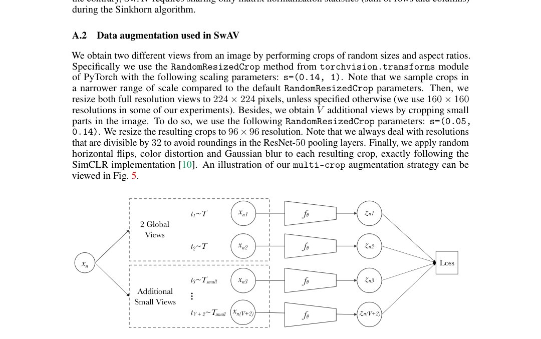
Figure 5: Multi-crop: the image is transformed into views: two global views and small resolution zoomed views.
图 5:Multi-crop:图像 变换为 个视图:两个全局视图与 个小分辨率放大视图。
A.3 Implementation details of linear classification on ImageNet with ResNet-50
We obtain top-1 accuracy on ImageNet by training a linear classifier on top of frozen final representations (-D) of a ResNet- trained with SwAV. This linear layer is trained during epochs, with a learning rate of and a weight decay of . We use cosine learning rate decay and a batch size of . We use standard data augmentations, i.e., cropping of random sizes and aspect ratios (default parameters of RandomResizedCrop) and random horizontal flips.
A.3 在 ImageNet 上用 ResNet-50 做线性分类的实现细节
我们在用 SwAV 训练的 ResNet- 的冻结最终表示( 维)上训练线性分类器,得到 ImageNet top-1 准确率 。该线性层训 个 epoch,学习率 ,权重衰减 ,余弦学习率衰减,batch 。使用标准数据增强,即随机大小与宽高比裁剪(RandomResizedCrop 默认参数)与随机水平翻转。
A.4 Implementation details of semi-supervised learning (finetuning with 1% or 10% labels)
We finetune with either 1% or 10% of ImageNet labeled images a ResNet- pretrained with SwAV. We use the 1% and 10% splits specified in the official code release of SimCLR. We mostly follow hyperparameters from PCL [37]: we train during epochs with a batch size of , we use distinct learning rates for the convnet weights and the final linear layer, and we decay the learning rates by a factor at epochs and . We do not apply any weight decay during finetuning. For 1% finetuning, we use a learning rate of for the trunk and for the final layer. For 10% finetuning, we use a learning rate of for the trunk and for the final layer.
A.4 半监督学习实现细节(用 1% 或 10% 标签微调)
我们用 ImageNet 有标签图像的 1% 或 10% 微调用 SwAV 预训练的 ResNet-。1% 与 10% 划分取自 SimCLR 官方代码发布。超参数大体遵循 PCL [37]:训 个 epoch、batch ,对卷积网络权重与最终线性层使用不同学习率,并在第 与 个 epoch 将学习率乘 。微调时不加权重衰减。1% 微调时 trunk 学习率 、最终层 ;10% 微调时 trunk 、最终层 。
A.5 Implementation details of transfer learning on downstream tasks
Linear classifiers. We mostly follow PIRL [44] for training linear models on top of representations given by a ResNet-50 pretrained with SwAV. On VOC07, all images are resized to 256 pixels along the shorter side, before taking a center crop. Then, we train a linear SVM with LIBLINEAR [18] on top of corresponding global average pooled final representations (-D). For linear evaluation on other datasets (Places205 and iNat18), we train linear models with stochastic gradient descent using a batch size of , a learning rate of reduced by a factor of three times (equally spaced intervals), weight decay of and momentum of . On Places205, we train the linear models for epochs and on iNat18 for epochs. We report the top-1 accuracy computed using the center crop on the validation set.
A.5 下游任务迁移学习实现细节
线性分类器。 在用 SwAV 预训练的 ResNet-50 表示上训练线性模型时,我们大体遵循 PIRL [44]。在 VOC07 上,所有图像沿短边缩放到 256 像素,再取 中心裁剪。然后用 LIBLINEAR [18] 在对应全局平均池化最终表示( 维)上训练线性 SVM。其他数据集(Places205 与 iNat18)的线性评估用随机梯度下降,batch ,学习率 三次等间隔乘 ,权重衰减 ,动量 。Places205 训 个 epoch,iNat18 训 个 epoch。报告验证集上用 中心裁剪计算的 top-1 准确率。
Object Detection on VOC07+12. We use a Faster R-CNN [50] model as implemented in Detectron2 [57] and follow the finetuning protocol from He et al. [24] making the following changes to the hyperparameters – our initial learning rate is which is warmed with a slope (WARMUP_FACTOR flag in Detectron2) of for iterations. Other training hyperparamters are kept exactly the same as in He et al. [24], i.e., batchsize of across GPUs, training for K iterations on VOC07+12 trainval with the learning rate reduced by a factor of after K and K iterations, using SyncBatchNorm to finetune BatchNorm parameters, and adding an extra BatchNorm layer after the res5 layer (Res5ROIHeadsExtraNorm head in Detectron2). We report results on VOC07 test set averaged over independant runs.
VOC07+12 目标检测。 我们使用 Detectron2 [57] 中实现的 Faster R-CNN [50],并遵循 He 等人 [24] 的微调协议,对超参数做如下改动——初始学习率 ,以 Detectron2 的 WARMUP_FACTOR 标志斜率 预热 次迭代。其余训练超参数与 He 等人 [24] 完全相同,即 8 GPU 上 batch ,在 VOC07+12 trainval 上训 K 次迭代,学习率在 K 与 K 后乘 ,用 SyncBatchNorm 微调 BatchNorm 参数,并在 res5 层后加额外 BatchNorm(Detectron2 的 Res5ROIHeadsExtraNorm)。在 VOC07 测试集上报告 5 次独立运行的平均结果。
Object Detection on COCO. We test the generalization of our ResNet-50 features trained on ImageNet with SwAV by transferring them to object detection on COCO dataset [38] with DETR framework [6]. DETR is a recent object detection framework that relies on a transformer encoder-decoder architecture. It reaches competitive performance with Faster R-CNN while being conceptually simpler and trainable end-to-end. Interestingly, unlike other frameworks [25], current results with DETR have shown that using a pretrained backbone is crucial to obtain good results compared to training from scratch. Therefore, we investigate if we can boost DETR performance by using features pretrained on ImageNet with SwAV instead of standard supervised features. We also evaluate features from MoCov2 [11] pretraining. We train DETR during epochs with AdamW, we use a learning rate of for the transformer and apply a weight decay of . We select for each method the best learning rate for the backbone among the following three values: , and . We decay the learning rates by a factor after epochs.
COCO 目标检测。 我们用 DETR 框架 [6] 把在 ImageNet 上用 SwAV 训练的 ResNet-50 特征迁移到 COCO 数据集 [38] 上的目标检测,以测试泛化。DETR 是近期依赖 transformer 编码器–解码器架构的目标检测框架,在概念更简单且可端到端训练的同时达到与 Faster R-CNN 竞争的表现。有趣的是,与其他框架 [25] 不同,当前 DETR 结果表明相对从头训练,使用预训练骨干对获得良好结果至关重要。因此我们研究用 ImageNet 上 SwAV 预训练特征替代标准有监督特征能否提升 DETR。我们也评估 MoCov2 [11] 预训练特征。我们用 AdamW 训 DETR 个 epoch,transformer 学习率 ,权重衰减 。对每种方法,从以下三个值中为骨干选择最佳学习率:、 与 。 个 epoch 后将学习率乘 。
A.6 Implementation details of training with small batches of 256 images
We start using a queue composed of the feature representations from previous batches after epochs of training. Indeed, we find that using the queue before epochs disturbs the convergence of the model since the network is changing a lot from an iteration to another during the first epochs. We simulate large batches of size by storing the last batches, that is vectors of dimension . We use a weight decay of , LARS optimizer [64] and a learning rate of . We use the cosine learning rate decay [40] with a final value of .
A.6 用 256 张图像小批次训练的实现细节
我们在训练 个 epoch 之后开始使用由先前批次特征表示组成的队列。确实,我们发现 个 epoch 前使用队列会干扰模型收敛,因为前几个 epoch 网络在迭代间变化很大。我们通过存储最近 个批次来模拟大小为 的大批次,即 个 维向量。权重衰减 ,LARS 优化器 [64],学习率 。使用终值为 的余弦学习率衰减 [40]。
A.7 Implementation details of ablation studies
In our ablation studies (results in Table of the main paper for example), we choose to follow closely the data augmentation used in concurrent work SimCLR. This allows a fair comparison and importantly, isolates the effect of our contributions. In practice, it means that we use the default parameters of the random crop method (RandomResizedCrop), s=(0.08, 1) instead of s=(0.14, 1), when sampling the two large resolution views.
A.7 消融研究实现细节
在消融研究中(例如主文表 的结果),我们选择紧密遵循同期工作 SimCLR 所用数据增强。这便于公平比较,并重要地把贡献的效果隔离出来。实践上,这意味着在采样两个大分辨率视图时,使用随机裁剪方法(RandomResizedCrop)的默认参数 s=(0.08, 1),而非 s=(0.14, 1)。
A.8 SimCLR loss with multi-crop augmentation
When implementing SimCLR with multi-crop augmentation, we have to deal with several positive pairs formed by an anchor features and the different crops coming from the same instance. We denote by the total number of unique dataset instances in the batch and by the number of crops per instance. For example, in the case of 2x160+4x96 crops, we have crops per instance. We call the effective total number of crops in the batch. Overall, we minimize the following loss
A.8 带 multi-crop 增强的 SimCLR 损失
实现带 multi-crop 增强的 SimCLR 时,需处理由锚点特征与来自同一实例的不同裁剪形成的多个正对。记 为批次中唯一数据集实例总数, 为每实例裁剪数。例如 2x160+4x96 裁剪时,每实例有 个裁剪。称 为批次中有效裁剪总数。总体最小化如下损失
For a feature representation , the corresponding set of positive examples is formed by the representations of the other crops from the same instance. The set of negatives is formed by the representations of all crops in the same batch except ones coming from the same instance as . Note that this extension of SimCLR loss with several pairs of positive is similar to the one used in Khosla et al. [33].
对特征表示 ,对应正例集合 由来自同一实例的其他裁剪表示构成。负例集合 由同批次中除来自与 相同实例外的全部裁剪表示构成。注意这种带多对正例的 SimCLR 损失扩展与 Khosla 等人 [33] 所用类似。
B Additional Results
B 补充结果
B.1 Running times
In table 4, we report compute and GPU memory requirements based on our implementation for different settings. As described in section A.1, we train each method on V100 16GB GPUs, with a batch size of , using mixed precision and apex optimized version of synchronized batch-normalization layers. We report results with ResNet- for all methods. In fig. 6, we report SwAV performance for different training lengths measured in hours based on our implementation. We observe that after only hours of training, SwAV outperforms SimCLR trained for epochs ( hours based on our implementation) by a large margin. If we train SwAV for longer, we see that the performance gap between the two methods increases even more.
B.1 运行时间
表 4 按我们的实现报告不同设定下的算力与 GPU 显存需求。如第 A.1 节所述,我们在 张 V100 16GB GPU 上、batch 、混合精度与 apex 优化同步批归一化层下训练各方法。全部方法报告 ResNet- 结果。图 6 按我们的实现、以小时计的不同训练时长报告 SwAV 表现。我们观察到仅训练 小时后,SwAV 便以大幅领先超过训 个 epoch 的 SimCLR(按我们实现约 小时)。若更长训练 SwAV,两方法间差距进一步拉大。
| Method | multi-crop | time / 100 epochs | peak memory / GPU |
|---|---|---|---|
| SimCLR | 4h00 | 8.6G | |
| SwAV | 4h09 | 8.6G | |
| SwAV | + | 4h50 | 8.5G |
| SwAV | + | 6h15 | 12.8G |
Table 4: Computational cost. We report time and GPU memory requirements based on our implementation for different models trained during epochs.
| 方法 | multi-crop | 每 100 epoch 时间 | 每 GPU 峰值显存 |
|---|---|---|---|
| SimCLR | 4h00 | 8.6G | |
| SwAV | 4h09 | 8.6G | |
| SwAV | + | 4h50 | 8.5G |
| SwAV | + | 6h15 | 12.8G |
表 4:计算开销。按我们的实现报告不同模型训 个 epoch 的时间与 GPU 显存需求。
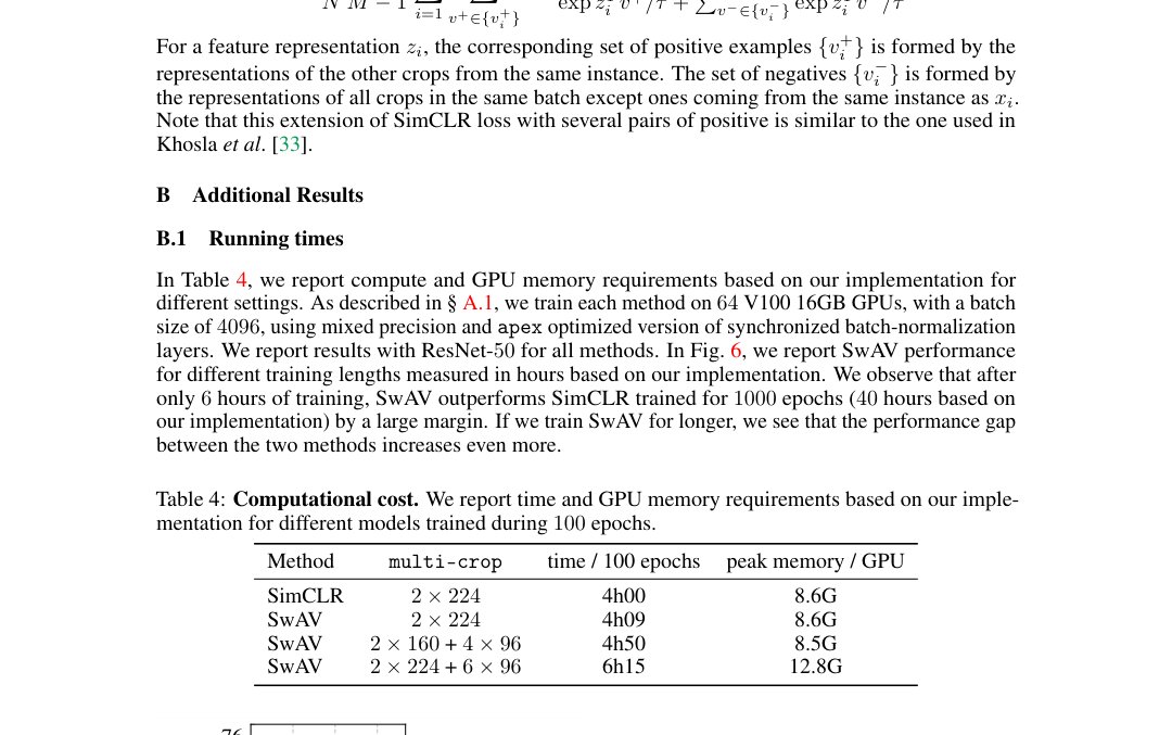
Figure 6: Influence of longer training. Top-1 ImageNet accuracy for linear models trained on frozen features. We report SwAV performance for different training lengths measured in hours based on our implementation. We train each ResNet- models on V100 16GB GPUs with a batch size of (see section A.1 for implementation details).
图 6:更长训练的影响。在冻结特征上训练线性模型的 ImageNet top-1 准确率。我们按实现以小时计报告不同训练时长下的 SwAV 表现。每个 ResNet- 在 张 V100 16GB GPU、batch 上训练(实现细节见第 A.1 节)。
B.2 Larger architectures
In table 5, we show results when training SwAV on large architectures. We observe that SwAV benefits from training on large architectures and plan to explore in this direction to furthermore boost self-supervised methods.
B.2 更大架构
表 5 展示在大架构上训练 SwAV 的结果。我们观察到 SwAV 受益于在大架构上训练,并计划沿此方向探索以进一步提升自监督方法。
| Method | Arch. | Param. | Top1 |
|---|---|---|---|
| Supervised | EffNet-B7 | 66 | 84.4 |
| Rotation [20] | RevNet50-4w | 86 | 55.4 |
| BigBiGAN [15] | RevNet50-4w | 86 | 61.3 |
| AMDIM [3] | Custom-RN | 626 | 68.1 |
| CMC [52] | R50-w2 | 188 | 68.4 |
| MoCo [24] | R50-w4 | 375 | 68.6 |
| CPC v2 [28] | R161 | 305 | 71.5 |
| SimCLR [10] | R50-w4 | 375 | 76.8 |
| SwAV | R50-w2 | 188 | 77.3 |
| SwAV | R50-w4 | 375 | 77.9 |
| SwAV | R50-w5 | 586 | 78.5 |
Table 5: Large architectures. Top-1 accuracy for linear models trained on frozen features from different self-supervised methods on large architectures.
| 方法 | 架构 | 参数量 | Top1 |
|---|---|---|---|
| Supervised | EffNet-B7 | 66 | 84.4 |
| Rotation [20] | RevNet50-4w | 86 | 55.4 |
| BigBiGAN [15] | RevNet50-4w | 86 | 61.3 |
| AMDIM [3] | Custom-RN | 626 | 68.1 |
| CMC [52] | R50-w2 | 188 | 68.4 |
| MoCo [24] | R50-w4 | 375 | 68.6 |
| CPC v2 [28] | R161 | 305 | 71.5 |
| SimCLR [10] | R50-w4 | 375 | 76.8 |
| SwAV | R50-w2 | 188 | 77.3 |
| SwAV | R50-w4 | 375 | 77.9 |
| SwAV | R50-w5 | 586 | 78.5 |
表 5:大架构。不同自监督方法在大架构冻结特征上训练线性模型的 top-1 准确率。
Implementation details for SwAV R50-w2.
The model is trained for epochs on GPUS (batch size ). We train the model with 2x224+4x96 (total of crops). All other hyperparameters are the same as the ones described in appendix A.1.
SwAV R50-w2 实现细节
模型在 张 GPU 上训 个 epoch(batch ),用 2x224+4x96(共 个裁剪)。其余超参数与附录 A.1 所述相同。
Implementation details for SwAV R50-w4.
The model is trained for epochs on GPUS (batch size ) with a queue of samples starting from the beginning of training. We train the model with 2x224+4x96 (total of crops). All other hyperparameters are the same as the ones described in appendix A.1.
SwAV R50-w4 实现细节
模型在 张 GPU 上训 个 epoch(batch ),自训练开始起使用大小为 样本的队列,用 2x224+4x96(共 个裁剪)。其余超参数与附录 A.1 所述相同。
Implementation details for SwAV R50-w5.
The model is trained for epochs on GPUS (batch size ) with a queue of samples starting from the beginning of training. We train the model with 2x224+4x96 (total of crops). All other hyperparameters are the same as the ones described in appendix A.1.
SwAV R50-w5 实现细节
模型在 张 GPU 上训 个 epoch(batch ),自训练开始起使用大小为 样本的队列,用 2x224+4x96(共 个裁剪)。其余超参数与附录 A.1 所述相同。
B.3 Transferring unsupervised features to downstream tasks
In table 6, we expand results from the main paper by providing numbers from previously and concurrently published self-supervised methods. In the left panel of table 6, we show performance after training a linear classifier on top of frozen representations on different datasets while on the right panel we evaluate the features by finetuning a ResNet- on object detection with Faster R-CNN [50] and DETR [6]. Overall, we observe on table 6 that SwAV is the first self-supervised method to outperform ImageNet supervised backbone on all the considered transfer tasks and datasets. Other self-supervised learners are capable of surpassing the supervised counterpart but only for one type of transfer (object detection with finetuning for MoCo/PIRL for example). We will release this model so other researchers might also benefit by replacing the ImageNet supervised network with our model.
B.3 把无监督特征迁移到下游任务
表 6 扩展主文结果,给出先前与同期发表的自监督方法的数值。表 6 左栏展示在不同数据集上冻结表示上训练线性分类器后的表现;右栏用 Faster R-CNN [50] 与 DETR [6] 微调 ResNet- 评估目标检测特征。总体看表 6,SwAV 是首个在全部考虑的迁移任务与数据集上超过 ImageNet 有监督骨干的自监督方法。其他自监督学习器能超过有监督对照,但仅在一种迁移类型上(例如 MoCo/PIRL 的微调目标检测)。我们将发布该模型,以便其他研究者也可用我们的模型替换 ImageNet 有监督网络获益。
| Linear Classification | Object Detection | ||||||
|---|---|---|---|---|---|---|---|
| Places205 | VOC07 | iNat18 | VOC07+12 | COCO | COCO | ||
| (Faster R-CNN R50-C4) | (Mask R-CNN R50-FPN) | (DETR) | |||||
| Supervised | |||||||
| RotNet [19] | - | - | - | ||||
| NPID++ [44] | - | ||||||
| MoCo [24] | - | ||||||
| PIRL [44] | - | ||||||
| PCL [37] | - | - | - | ||||
| BoWNet [19] | - | - | |||||
| SimCLR [10] | - | - | |||||
| MoCov2 [24] | |||||||
| SwAV |
Table 6: Transfer learning on downstream tasks. Comparison between features from ResNet-50 trained on ImageNet with SwAV or supervised learning. We also report numbers from other self-supervised methods († for numbers from other methods run by us). We consider two settings. (1) Linear classification on top of frozen features. We report top-1 accuracy on all datasets except VOC07 where we report mAP. (2) Object detection with finetuned features on VOC07+12 trainval using Faster R-CNN [50] and on COCO [38] using Mask R-CNN [26] or DETR [6]. We report the most standard detection metrics for these datasets: on VOC07+12 and AP on COCO.
| 线性分类 | 目标检测 | ||||||
|---|---|---|---|---|---|---|---|
| Places205 | VOC07 | iNat18 | VOC07+12 | COCO | COCO | ||
| (Faster R-CNN R50-C4) | (Mask R-CNN R50-FPN) | (DETR) | |||||
| Supervised | |||||||
| RotNet [19] | - | - | - | ||||
| NPID++ [44] | - | ||||||
| MoCo [24] | - | ||||||
| PIRL [44] | - | ||||||
| PCL [37] | - | - | - | ||||
| BoWNet [19] | - | - | |||||
| SimCLR [10] | - | - | |||||
| MoCov2 [24] | |||||||
| SwAV |
表 6:下游任务上的迁移学习。比较在 ImageNet 上用 SwAV 或有监督学习训练的 ResNet-50 特征。也报告其他自监督方法的数值(† 表示我们复现的其他方法数值)。考虑两种设定。(1) 冻结特征上的线性分类。除 VOC07 报告 mAP 外,其余数据集报告 top-1 准确率。(2) 用 Faster R-CNN [50] 在 VOC07+12 trainval、用 Mask R-CNN [26] 或 DETR [6] 在 COCO [38] 上微调特征做目标检测。报告这些数据集最常用的检测指标:VOC07+12 的 与 COCO 的 AP。
B.4 More detection metrics for object detection
In table 7, table 8 and table 9, we evaluate the features by finetuning a ResNet- with different detectors: Mask R-CNN [26], Faster R-CNN [50] and DETR [6]. We report more detection metrics compared to the table in the main paper table 6. We observe in table 7, table 8 and in table 9 that SwAV outperforms the ImageNet supervised pretrained model on all the detection evaluation metrics.
B.4 目标检测的更多检测指标
表 7、表 8 与表 9 用不同检测器微调 ResNet- 评估特征:Mask R-CNN [26]、Faster R-CNN [50] 与 DETR [6]。相对主文表 6,我们报告更多检测指标。表 7、表 8 与表 9 显示,SwAV 在全部检测评估指标上超过 ImageNet 有监督预训练模型。
Note that MoCov2 backbone performs particularly well on the object detection benchmark, and even outperform SwAV features for some detection metrics. However, as shown in table 6, this backbone is not competitive with the supervised features when evaluating on classification tasks without finetuning.
注意 MoCov2 骨干在目标检测基准上表现尤其好,部分检测指标甚至超过 SwAV 特征。但如表 6 所示,在不做微调的分类任务上评估时,该骨干无法与有监督特征竞争。
| Method | APb | AP | AP | APm | AP | AP |
|---|---|---|---|---|---|---|
| Supervised | 39.7 | 59.5 | 43.3 | 35.9 | 56.6 | 38.6 |
| MoCo-v2 [11] | 39.8 | 59.8 | 43.6 | 36.1 | 56.9 | 38.7 |
| SwAV | 41.6 | 62.3 | 45.5 | 37.8 | 59.6 | 40.5 |
Table 7: Object detection and instance segmentation finetuned on COCO. Following the setup of [24], we use Mask R-CNN detector with ResNet50-FPN trained on train2017 with default schedule and evaluated on val2017. The metrics include bounding box AP (AP) and mask AP (AP).
| 方法 | APb | AP | AP | APm | AP | AP |
|---|---|---|---|---|---|---|
| Supervised | 39.7 | 59.5 | 43.3 | 35.9 | 56.6 | 38.6 |
| MoCo-v2 [11] | 39.8 | 59.8 | 43.6 | 36.1 | 56.9 | 38.7 |
| SwAV | 41.6 | 62.3 | 45.5 | 37.8 | 59.6 | 40.5 |
表 7:在 COCO 上微调的目标检测与实例分割。遵循 [24] 设定,使用带 ResNet50-FPN 的 Mask R-CNN 检测器,在 train2017 上按默认 日程训练并在 val2017 上评估。指标包括框 AP(AP)与掩码 AP(AP)。
| Method | APall | AP50 | AP75 |
|---|---|---|---|
| Supervised | 53.5 | 81.3 | 58.8 |
| Random | 28.1 | 52.5 | 26.2 |
| NPID++ [44] | 52.3 | 79.1 | 56.9 |
| PIRL [44] | 54.0 | 80.7 | 59.7 |
| BoWNet [19] | 55.8 | 81.3 | 61.1 |
| MoCov1 [24] | 55.9 | 81.5 | 62.6 |
| MoCov2 [11] | 57.4 | 82.5 | 64.0 |
| SwAV | 56.1 | 82.6 | 62.7 |
Table 8: More detection metrics for object detection on VOC07+12 with finetuned features using Faster R-CNN [50].
| 方法 | APall | AP50 | AP75 |
|---|---|---|---|
| Supervised | 53.5 | 81.3 | 58.8 |
| Random | 28.1 | 52.5 | 26.2 |
| NPID++ [44] | 52.3 | 79.1 | 56.9 |
| PIRL [44] | 54.0 | 80.7 | 59.7 |
| BoWNet [19] | 55.8 | 81.3 | 61.1 |
| MoCov1 [24] | 55.9 | 81.5 | 62.6 |
| MoCov2 [11] | 57.4 | 82.5 | 64.0 |
| SwAV | 56.1 | 82.6 | 62.7 |
表 8:用 Faster R-CNN [50] 在 VOC07+12 上微调特征做目标检测的更多指标。
| Method | AP | ||||||
|---|---|---|---|---|---|---|---|
| ImageNet labels | 40.8 | 61.2 | 42.9 | 20.1 | 44.5 | 60.3 | |
| MoCo-v2 | 42.0 | 62.7 | 44.4 | 20.8 | 45.6 | 60.9 | |
| SwAV | 42.1 | 63.1 | 44.5 | 19.7 | 46.3 | 60.9 |
Table 9: More detection metrics for object detection on COCO with finetuned features using DETR [6].
| 方法 | AP | ||||||
|---|---|---|---|---|---|---|---|
| ImageNet labels | 40.8 | 61.2 | 42.9 | 20.1 | 44.5 | 60.3 | |
| MoCo-v2 | 42.0 | 62.7 | 44.4 | 20.8 | 45.6 | 60.9 | |
| SwAV | 42.1 | 63.1 | 44.5 | 19.7 | 46.3 | 60.9 |
表 9:用 DETR [6] 在 COCO 上微调特征做目标检测的更多指标。
B.5 Low-Shot learning on ImageNet for SwAV pretrained on Instagram data
We now test whether SwAV pretrained on Instagram data can serve as a pretraining method for low-shot learning on ImageNet. We report in table 9 results when finetuning Instagram SwAV features with only few labels per ImageNet category. We observe that using pretrained features from Instagram improves considerably the performance compared to training from scratch.
B.5 在 Instagram 数据上预训练的 SwAV 在 ImageNet 上的低样本学习
我们接着测试在 Instagram 数据上预训练的 SwAV 能否作为 ImageNet 低样本学习的预训练方法。表 10 报告仅用每类少量标签微调 Instagram SwAV 特征的结果。我们观察到相对从头训练,使用 Instagram 预训练特征可大幅提升表现。
| # examples per class | 13 | 128 | ||
|---|---|---|---|---|
| top1 | top5 | top1 | top5 | |
| No pretraining | 25.4 | 48.4 | 56.4 | 80.4 |
| SwAV IG-1B | 38.2 | 67.1 | 64.7 | 87.2 |
Table 10: Low-shot learning on ImageNet. Top-1 and top-5 accuracies when training with or examples per category.
| 每类样本数 | 13 | 128 | ||
|---|---|---|---|---|
| top1 | top5 | top1 | top5 | |
| No pretraining | 25.4 | 48.4 | 56.4 | 80.4 |
| SwAV IG-1B | 38.2 | 67.1 | 64.7 | 87.2 |
表 10:ImageNet 低样本学习。每类用 或 个样本训练时的 top-1 与 top-5 准确率。
B.6 Image classification with KNN classifiers on ImageNet
Following previous work protocols [58, 68], we evaluate the quality of our unsupervised features with K-nearest neighbor (KNN) classifiers on ImageNet. We get features from the computed network outputs for center crops of training and test images. We report results with and NN in table 11. We outperform the current state-of-the-art of this evaluation. Interestingly we also observe that using fewer NN actually boosts the performance of our model.
B.6 在 ImageNet 上用 KNN 分类器做图像分类
遵循先前工作协议 [58, 68],我们用 ImageNet 上的 K 近邻(KNN)分类器评估无监督特征质量。对训练与测试图像的中心裁剪取网络输出作为特征。表 11 报告 与 近邻的结果。我们超过该评估的当前最优。有趣的是,我们也观察到使用更少近邻实际上提升了我们模型的表现。
| Method | 20-NN | 200-NN | |
|---|---|---|---|
| NPID [58] | - | 46.5 | |
| LA [68] | - | 49.4 | |
| PCL [37] | 54.5 | - | |
| SwAV | 65.7 | 62.7 |
Table 11: KNN classifiers on ImageNet. We report top-1 accuracy with and nearest neighbors.
| 方法 | 20-NN | 200-NN | |
|---|---|---|---|
| NPID [58] | - | 46.5 | |
| LA [68] | - | 49.4 | |
| PCL [37] | 54.5 | - | |
| SwAV | 65.7 | 62.7 |
表 11:ImageNet 上的 KNN 分类器。报告 与 近邻的 top-1 准确率。
C Ablation Studies on Clustering
C 聚类消融研究
C.1 Number of prototypes
In table 12, we evaluate the influence of the number of prototypes used in SwAV. We train ResNet-50 with SwAV for epochs with crops (ablation study setting) and evaluate the performance by training a linear classifier on top of frozen final representations. We observe in table 12 that varying the number of prototypes by an order of magnitude (3k-100k) does not affect much the performance (at most on ImageNet). This suggests that the number of prototypes has little influence as long as there are “enough”. Throughout the paper, we train SwAV with prototypes. We find that using more prototypes increases the computational time both in the Sinkhorn algorithm and during back-propagation for an overall negligible gain in performance.
C.1 原型数量
表 12 评估 SwAV 所用原型数量的影响。我们在消融设定下用 裁剪、SwAV 训 ResNet-50 个 epoch,并在冻结最终表示上训练线性分类器评估表现。表 12 显示,原型数在一个数量级内变化(3k–100k)对表现影响不大(ImageNet 上最多 )。这表明只要“足够多”,原型数量影响很小。全文我们用 个原型训练 SwAV。我们发现更多原型会增加 Sinkhorn 算法与反向传播的计算时间,而整体收益可忽略。
| Number of prototypes | 300 | 1000 | 3000 | 10000 | 30000 | 100000 |
|---|---|---|---|---|---|---|
| Top-1 | 72.8 | 73.6 | 73.9 | 74.1 | 73.8 | 73.8 |
Table 12: Impact of number of prototypes. Top-1 ImageNet accuracy for linear models trained on frozen features.
| 原型数量 | 300 | 1000 | 3000 | 10000 | 30000 | 100000 |
|---|---|---|---|---|---|---|
| Top-1 | 72.8 | 73.6 | 73.9 | 74.1 | 73.8 | 73.8 |
表 12:原型数量的影响。在冻结特征上训练线性模型的 ImageNet top-1 准确率。
C.2 Learning the prototypes
We investigate the impact of learning the prototypes compared to using fixed random prototypes. Assigning features to fixed random targets has been explored in NAT [5]. However, unlike SwAV, NAT uses a target per instance in the dataset, the assignment is hard and performed with Hungarian algorithm. In table 13 (left), we observe that learning prototypes improves SwAV from to which shows the effect of adapting the prototypes to the dataset distribution.
C.2 学习原型
我们研究学习原型相对使用固定随机原型的影响。把特征分配到固定随机目标已在 NAT [5] 中探索。但与 SwAV 不同,NAT 对数据集中每个实例使用一个目标,分配是硬分配,并用匈牙利算法完成。表 13(左)显示,学习原型把 SwAV 从 提升到 ,表明使原型适应数据分布有效果。
Overall, these results suggest that our framework learns from a different signal from "offline" approaches that attribute a pseudo-label to each instance while considering the full dataset and then predict these labels (like DeepCluster [7] for example). Indeed, the prototypes in SwAV are not strongly encouraged to be categorical and random fixed prototypes work almost as well. Rather, they help contrasting different image views without relying on pairwise comparison with many negatives samples. This might explain why the number of prototypes does not impact the performance significantly.
总体而言,这些结果表明我们的框架所学信号不同于“离线”方法——后者在考虑全数据集时为每个实例赋伪标签再预测这些标签(例如 DeepCluster [7])。确实,SwAV 中的原型并不被强烈鼓励成为类别型,随机固定原型几乎同样好。它们更多是在不依赖与大量负样本成对比较的情况下帮助对比不同图像视图。这或许可以解释为何原型数量对表现影响不显著。
| Prototypes | Learned | Fixed |
|---|---|---|
| Top-1 | 73.9 | 73.1 |
| Assignment | Soft | Hard |
|---|---|---|
| Top-1 | 73.9 | 73.3 |
Table 13: Ablation studies on clustering. Top-1 ImageNet accuracy for linear models trained on frozen features. (left) Impact of learning the prototypes. (right) Hard versus soft assignments.
| 原型 | 学习 | 固定 |
|---|---|---|
| Top-1 | 73.9 | 73.1 |
| 分配 | 软 | 硬 |
|---|---|---|
| Top-1 | 73.9 | 73.3 |
表 13:聚类消融研究。在冻结特征上训练线性模型的 ImageNet top-1 准确率。(左) 学习原型的影响。(右) 硬分配与软分配。
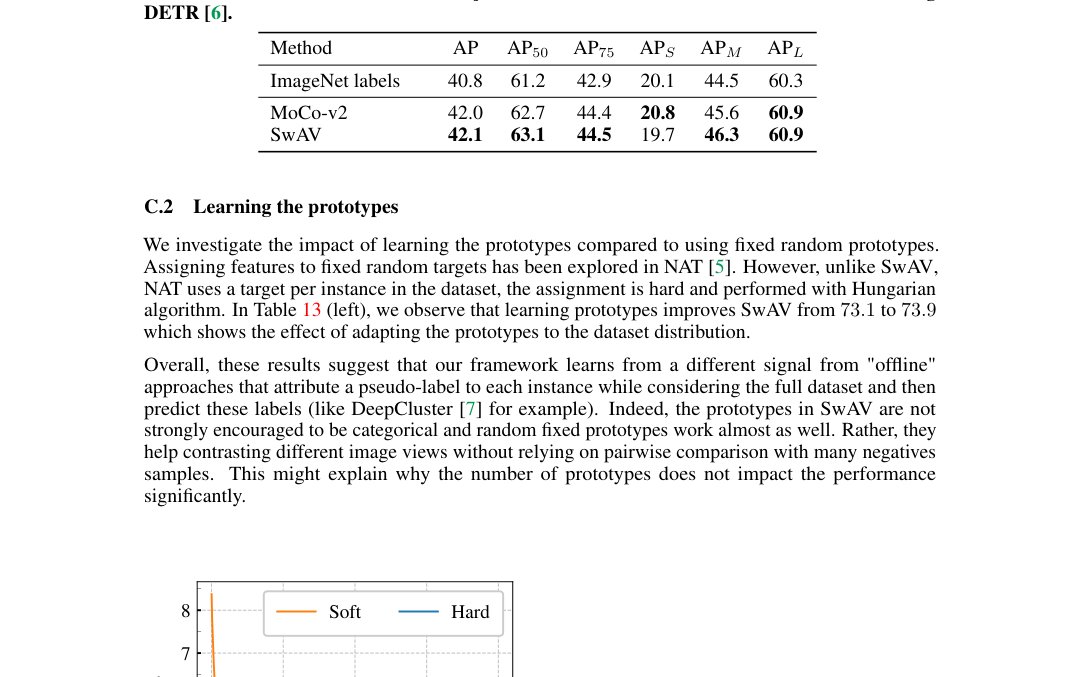
Figure 7: Hard versus soft assignments. We report the training loss for SwAV models trained with either soft or hard assignments. The models are trained during epochs with crops.
图 7:硬分配与软分配。报告分别用软或硬分配训练的 SwAV 模型的训练损失。模型用 裁剪训 个 epoch。
C.3 Hard versus soft assignments
In table 13 (right), we evaluate the impact of using hard assignment instead of the default soft assignment in SwAV. We train the models during epochs with crops (ablation study setting) and evaluate the performance by training a linear classifier on top of frozen final representations. We also report the training losses in fig. 7. We observe that using the hard assignments performs worse than using the soft assignments. An explanation is that the rounding needed to obtain discrete codes is a more aggressive optimization step than gradient updates. While it makes the model converge rapidly (see fig. 7), it leads to a worse solution.
C.3 硬分配与软分配
表 13(右)评估在 SwAV 中用硬分配替代默认软分配的影响。我们在消融设定下用 裁剪训模型 个 epoch,并在冻结最终表示上训练线性分类器评估。图 7 也报告训练损失。我们观察到硬分配表现差于软分配。一种解释是:为得到离散码所需的取整是比梯度更新更激进的优化步骤。虽使模型收敛更快(见图 7),却导向更差解。
| Sinkhorn iterations | 1 | 3 | 10 | 30 |
|---|---|---|---|---|
| Top-1 | fail | 73.9 | 73.8 | 73.7 |
Table 14: Impact of the number of iterations in Sinkhorn algorithm. Top-1 ImageNet accuracy for linear models trained on frozen features.
| Sinkhorn 迭代次数 | 1 | 3 | 10 | 30 |
|---|---|---|---|---|
| Top-1 | fail | 73.9 | 73.8 | 73.7 |
表 14:Sinkhorn 算法迭代次数的影响。在冻结特征上训练线性模型的 ImageNet top-1 准确率。
C.4 Impact of the number of iterations in Sinkhorn algorithm
In table 14, we investigate the impact of the number of normalization steps performed during Sinkhorn-Knopp algorithm [13] on the performance of SwAV. We observe that using only iterations is enough for the model to converge. When performing less iterations, the loss fails to converge. We observe that using more iterations slightly alters the transfer performance of the model. We conjecture that it is for the same reason that rounding codes to discrete values deteriorate the quality of our model by converging too rapidly.
C.4 Sinkhorn 算法迭代次数的影响
表 14 研究 Sinkhorn-Knopp 算法 [13] 中归一化步数对 SwAV 表现的影响。我们观察到仅 次迭代已足以使模型收敛。迭代更少时损失无法收敛。更多迭代会略微损害模型的迁移表现。我们推测这与把码取整为离散值会因收敛过快而损害模型质量出于同一原因。
D Details on Clustering-Based methods: DeepCluster-v2 and SeLa-v2
D 基于聚类方法的细节:DeepCluster-v2 与 SeLa-v2
In this section, we provide details on our improved implementation of clustering-based approaches DeepCluster-v2 and SeLa-v2 compared to their corresponding original publications [7, 2]. These two methods follow the same pipeline: they alternate between pseudo-labels generation (“assignment phase”) and training the network with a classification loss supervised by these pseudo-labels (“training phase”).
本节给出相对原发表 [7, 2] 改进后的基于聚类方法 DeepCluster-v2 与 SeLa-v2 的实现细节。这两种方法遵循同一流水线:在伪标签生成(“分配阶段”)与用这些伪标签监督的分类损失训练网络(“训练阶段”)之间交替。
D.1 Training phase
During the training phase, both methods minimize the multinomial logistic loss of the pseudo-labels classification problem:
D.1 训练阶段
训练阶段,两种方法都最小化伪标签 分类问题的多项逻辑损失:
The pseudo-labels are kept fixed during training and updated for the entire dataset once per epoch during the assignment phase.
训练期间伪标签保持固定,并在分配阶段每个 epoch 对整个数据集更新一次。
Training phase in DeepCluster-v2.
In the original DeepCluster work, both the classification head and the convnet weights are trained to classify the images into their corresponding pseudo-label between two assignments. Intuitively, this classification head is optimized to represent prototypes for the different pseudo-classes. However, since there is no mapping between two consecutive assignments: the classification head learned during an assignment becomes irrelevant for the following one. Thus, this classification head needs to be re-set at each new assignment which considerably disrupts the convnet training. For this reason, we propose to simply use for classification head the centroids given by k-means clustering (Eq. 11). Overall, during training, DeepCluster-v2 optimizes the following problem with mini-batch SGD:
DeepCluster-v2 的训练阶段。
原 DeepCluster 工作中,分类头 与卷积网络权重都在两次分配之间被训练,以把图像分到对应伪标签。直观上,该分类头被优化为表示不同伪类的原型。但由于两次连续分配之间没有映射:一次分配上学到的分类头对下一次变得无关。因此每次新分配都需重置分类头,严重干扰卷积网络训练。为此,我们建议分类头 直接使用 k-means 聚类给出的中心(式 11)。总体在训练时,DeepCluster-v2 用小批量 SGD 优化如下问题:
Training phase in SeLa-v2.
In SeLa work, the prototypes are learned with stochastic gradient descend during the training phase. Overall, during training, SeLa-v2 optimizes the following problem:
SeLa-v2 的训练阶段。
在 SeLa 工作中,原型 在训练阶段用随机梯度下降学习。总体在训练时,SeLa-v2 优化如下问题:
D.2 Assignment phase
The purpose of the assignment phase is to provide assignments for each instance of the dataset. For both methods, this implies having access to feature representations for the entire dataset. Both original works [7, 2] perform regularly a pass forward on the whole dataset to get these features. Using the original implementation, if assignments are updated at each epoch, then the assignment phase represents one third of the total training time. Therefore, in order to speed up training, we choose to use the features computed during the previous epoch instead of dedicating pass forwards to the assignments. This is similar to the memory bank introduced by Wu et al. [58], without momentum.
D.2 分配阶段
分配阶段的目的是为数据集每个实例提供分配 。对两种方法,这都意味着需要访问整个数据集的特征表示 。原工作 [7, 2] 都定期对整个数据集做前向以得到这些特征。用原实现若每个 epoch 更新分配,则分配阶段约占训练总时间的三分之一。因此为加速训练,我们选择使用上一 epoch 计算的特征,而非为分配专门做前向。这类似于 Wu 等人 [58] 引入的记忆库,但不带动量。
Assignment phase in DeepCluster-v2.
DeepCluster-v2 uses spherical k-means to get pseudo-labels. In particular, pseudo-labels are obtained by minimizing the following problem:
DeepCluster-v2 的分配阶段。
DeepCluster-v2 用球面 k-means 得到伪标签。具体地,伪标签 通过最小化如下问题得到:
where and the columns of are normalized. The original work DeepCluster uses tricks such as cluster re-assignments and balanced batch sampling to avoid trivial solutions but we found these unnecessary, and did not observe collapsing during our trainings. As noted by Asano et al., this is due to the fact that assignment and training are well separated phases.
其中 与 的列均已归一化。原工作 DeepCluster 使用聚类重分配与平衡批次采样等技巧以避免平凡解,但我们发现这些并非必要,训练中也未观察到坍缩。如 Asano 等人所指出,这是因为分配与训练是良好分离的阶段。
Assignment phase in SeLa-v2.
Unlike DeepCluster, SeLa uses the same loss during training and assignment phases. In particular, we use Sinkhorn-Knopp algorithm to optimize the following assignment problem (see details and derivations in the original SeLa paper [2]):
SeLa-v2 的分配阶段。
与 DeepCluster 不同,SeLa 在训练与分配阶段使用相同损失。具体地,我们用 Sinkhorn-Knopp 算法优化如下分配问题(细节与推导见原 SeLa 论文 [2]):
Implementation details
We use the same hyperparameters as SwAV to train SeLa-v2 and DeepCluster-v2: these are described in section A. Asano et al. [2] have shown that multi-clustering boosts performance of clustering-based approaches, and so we use sets of prototypes when training SeLa-v2 and DeepCluster-v2. Note that unlike online methods (like SwAV, SimCLR and MoCo), the clustering approaches SeLa-v2 and DeepCluster-v2 can be implemented with only a single crop per image per batch. The major limitation of SeLa-v2 and DeepCluster-v2 is that these methods are not online and therefore scaling them to very large scale dataset is not posible without major adjustments.
实现细节
我们用与 SwAV 相同的超参数训练 SeLa-v2 与 DeepCluster-v2:见第 A 节。Asano 等人 [2] 已表明多聚类提升基于聚类方法的表现,因此训练 SeLa-v2 与 DeepCluster-v2 时使用 组各 个原型 。注意与在线方法(如 SwAV、SimCLR 与 MoCo)不同,聚类方法 SeLa-v2 与 DeepCluster-v2 可在每个批次每张图像仅用单个裁剪实现。SeLa-v2 与 DeepCluster-v2 的主要局限是它们非在线,因此若不做重大调整,难以扩展到超大规模数据集。