Superposition Yields Robust Neural Scaling
Superposition Yields Robust Neural Scaling
Yizhou Liu Thanks: liuyz@mit.edu Ziming Liu Jeff Gore Affiliation: Massachusetts Institute of Technology Affiliation: Cambridge, MA 02139
Abstract
The success of today’s large language models (LLMs) depends on the observation that larger models perform better. However, the origin of this neural scaling law — the finding that loss decreases as a power law with model size — remains unclear. Starting from two empirical principles — that LLMs represent more things than the model dimensions (widths) they have (i.e., representations are superposed), and that words or concepts in language occur with varying frequencies — we constructed a toy model to study the loss scaling with model size. We found that when superposition is weak, meaning only the most frequent features are represented without interference, the scaling of loss with model size depends on the underlying feature frequency; if feature frequencies follow a power law, so does the loss. In contrast, under strong superposition, where all features are represented but overlap with each other, the loss becomes inversely proportional to the model dimension across a wide range of feature frequency distributions. This robust scaling behavior is explained geometrically: when many more vectors are packed into a lower dimensional space, the interference (squared overlaps) between vectors scales inversely with that dimension. We then analyzed four families of open-sourced LLMs and found that they exhibit strong superposition and quantitatively match the predictions of our toy model. The Chinchilla scaling law turned out to also agree with our results. We conclude that representation superposition is an important mechanism underlying the observed neural scaling laws. We anticipate that these insights will inspire new training strategies and model architectures to achieve better performance with less computation and fewer parameters.
当今大语言模型(LLM)的成功,依赖「更大模型表现更好」这一观察。但神经缩放律——损失随模型规模呈幂律下降——的起源仍不清楚。我们从两条经验原则出发:LLM 表示的事物多于其模型维数(宽度),即表征处于叠加(superposition);以及语言中词或概念出现频率不等。据此构造玩具模型,研究损失随模型规模的缩放。发现当叠加较弱——仅最频繁特征被无干扰地表示——时,损失随模型规模的缩放依赖底层特征频率:若特征频率服从幂律,损失亦然。相反,在强叠加下——所有特征都被表示但彼此重叠——在广泛的特征频率分布上,损失与模型维数成反比。这一稳健缩放可从几何解释:当远多于维数的向量被塞进低维空间时,向量间干扰(重叠平方)随该维数反比缩放。我们随后分析四个开源 LLM 家族,发现它们呈强叠加,并与玩具模型预测定量吻合;Chinchilla 缩放律也与结果一致。结论是:表征叠加是观测到的神经缩放律背后的重要机制。我们预期这些洞见将启发新的训练策略与模型结构,以更少计算与参数达到更好表现。
1 Introduction
The remarkable success of large language models (LLMs) has been driven by the empirical observation that increasing model size, training data, and compute consistently leads to better performance [1, 2, 3, 4]. Across a wide range of tasks — including language understanding [1, 5, 6], math [7, 8, 9, 10], and code generation [11, 12] — larger models achieve lower loss, higher accuracy, and greater generalization abilities [2, 13]. This consistent trend, known as neural scaling laws, has been observed across multiple model families and architectures, fueling the development of increasingly large models [2, 3, 4]. These scaling laws have not only shaped the current strategies for building better models but have also raised fundamental questions about why such simple and universal patterns emerge in complex learning systems.
大语言模型(LLM)的显著成功,由「增大模型规模、训练数据与算力会持续带来更好表现」这一经验观察驱动 [1, 2, 3, 4]。在语言理解 [1, 5, 6]、数学 [7, 8, 9, 10] 与代码生成 [11, 12] 等广泛任务上,更大模型损失更低、准确率更高、泛化更强 [2, 13]。这一一致趋势被称为神经缩放律,已在多个模型家族与架构上被观测到,并推动了越来越大的模型 [2, 3, 4]。缩放律不仅塑造了当前造更好模型的策略,也提出了根本问题:为何复杂学习系统中会出现如此简单而普遍的模式。
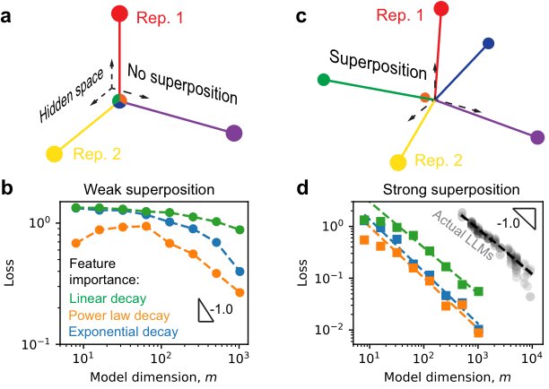
Figure 1: Superposition leads to robust and fast power-law loss decay with model size. (a) Illustration of no superposition where a three-dimensional space can at most represent three features without any interference (overlap). (b) Toy model results in the regime of weak superposition, where we set data dimension (number of features). The toy model will be introduced; more details are in Appendix D.1. (c) Illustration of superposition: there are more features than the dimension of the space. (d) The same toy models in the strong superposition regime show lower losses, which are on power laws with model dimension and have exponents close to (color coding same as panel b). The gray points are from actual LLMs, which seem to have a similar power-law relation with exponent .
图 1:叠加带来随模型规模稳健且快速的幂律损失衰减。(a)无叠加示意:三维空间最多无干扰(重叠)地表示三个特征。(b)弱叠加区玩具模型结果,数据维 (特征数)。玩具模型将在后文引入;更多细节见附录 D.1。(c)叠加示意:特征数多于空间维数。(d)同一玩具模型在强叠加区损失更低,相对模型维呈幂律且指数接近 (配色同面板 b)。灰色点来自真实 LLM,似乎也有指数 的类似幂律关系。
The scaling of loss with model size plays a central role in both the practical design and the theoretical understanding of large-scale machine learning systems, yet its origin remains inconclusive [3, 14, 15, 16, 17, 18, 19, 20, 21, 22, 23, 24]. Various explanations have been proposed, drawing from statistical learning theory and empirical phenomenological models, including improved function or manifold approximation in larger models [14, 15], and enhanced representation or skill learning in larger models [18, 19, 20, 21]. In the limit of infinite data, many of these explanations predict a power-law decay of loss with model size, provided the underlying data distribution also follows a power law. However, the predicted scaling exponents depend sensitively on the properties of the data distribution. Moreover, the connection between these mechanistic explanations and the behavior of actual LLMs needs further exploration.
损失随模型规模的缩放,在大规模机器学习系统的实践设计与理论理解中都居中心地位,但其起源仍无定论 [3, 14, 15, 16, 17, 18, 19, 20, 21, 22, 23, 24]。已有解释来自统计学习理论与经验唯象模型,包括更大模型中更好的函数或流形逼近 [14, 15],以及更强的表征或技能学习 [18, 19, 20, 21]。在无限数据极限下,许多解释在数据分布也服从幂律时,预测损失随模型规模幂律衰减;但预测的缩放指数对数据分布性质敏感。这些机制解释与真实 LLM 行为之间的联系仍需进一步探索。
When considering LLMs specifically, it becomes clear that representation learning can be a limiting factor, which is closely related to a phenomenon called superposition [25, 26], yet this aspect has not been thoroughly studied. LLMs must learn embedding vectors for tokens, process these representations through transformer layers to predict the next token, and use a final projection (the language model head) to generate the output. Conceptually, fitting functions or manifolds and learning skills or grammars are primarily tasks of the transformer layers, while representation learning is more directly tied to the embedding matrix and the language model head. To represent more than fifty thousand tokens — or even more abstract concepts — within a hidden space of at most a few thousand dimensions, the quality of representations is inevitably constrained, contributing to the final loss. Although models can represent more features than their dimensionality would suggest through a mechanism known as superposition [26], prior work on neural scaling laws has implicitly assumed weak superposition [15, 16, 17, 18, 19], which may be less relevant to the regime where LLMs operate. To address this gap, we systematically study here how representation superposition and data structure together influence the scaling of loss with model size.
具体到 LLM,表征学习可以成为限制因素,这与称为 叠加 的现象密切相关 [25, 26],但该方面尚未被充分研究。LLM 须为 token 学习嵌入向量,经 transformer 层处理这些表征以预测下一 token,再用最终投影(语言模型头)生成输出。概念上,拟合函数或流形、学习技能或语法主要是 transformer 层的任务,而表征学习更直接系于嵌入矩阵与语言模型头。要在至多数千维的隐空间中表示五万以上 token——乃至更多抽象概念——表征质量不可避免受约束,并贡献于最终损失。虽可通过叠加机制表示多于维数的特征 [26],先前神经缩放律工作常隐含假设弱叠加 [15, 16, 17, 18, 19],这可能与 LLM 实际所处区间不太相关。为填补缺口,我们在此系统研究表征叠加与数据结构如何共同影响损失随模型规模的缩放。
We adopt a toy model construction similar to [26] to study how superposition affects neural scaling laws. In the toy model, representations are learned by recovering data, each composed of multiple latent features. These features in data have different frequencies of occurrence, reflecting their relative importance. In the absence of superposition, only the most frequent features are perfectly represented, while the others are ignored. As illustrated in Figure 1a, the first three of six features are represented in the three-dimensional space without interference, and the remaining three are omitted. We find that in the weak superposition regime, the scaling of loss with model dimension depends sensitively on how feature frequency decays with rank: the loss follows a power law with model size only if the feature frequencies themselves follow a power law, provided that is sufficiently large (Figure 1b). By contrast, strong superposition allows many more features to be represented, albeit with overlap in the representation (Figure 1c). In this regime, the model displays a robust behavior: loss scales inversely with model dimension, independent of the data frequency distribution (Figure 1d). Remarkably, we find that actual LLMs follow the same rule. Comparing models with the same dimension but different superposition degrees, the ones with stronger superposition also have a lower loss. Building on the basic phenomena, we provide the main takeaways: (i) In the strong superposition regime, loss due to imperfect representation scales inversely with model dimension, largely independent of feature frequency distributions; (ii) Scaling behaviors in the weak superposition regime are brittle and depend on the number of activated but unlearned features, and in the strong superposition regime are robust and can be understood via generic geometric facts; (iii) LLMs exhibit strong superposition and agree quantitatively with our toy model predictions.
我们采用类似 [26] 的玩具模型构造,研究叠加如何影响神经缩放律。玩具模型通过恢复数据来学习表征,每条数据由多个潜在特征组成;这些特征出现频率不同,反映相对重要性。无叠加时,仅最频繁特征被完美表示,其余被忽略。如图 1a:六特征中前三在三维空间无干扰表示,后三省略。我们发现:在弱叠加区,损失随模型维的缩放对特征频率随秩衰减的方式敏感——仅当特征频率本身服从幂律且 足够大时,损失才随模型规模呈幂律(图 1b)。相反,强叠加允许表示远更多特征,但表征有重叠(图 1c)。在此区间模型表现稳健:损失与模型维成反比,且独立于数据频率分布(图 1d)。更惊人的是,真实 LLM 遵循同一规则;同维但叠加程度不同时,叠加更强者损失更低。基于这些基本现象,主要要点为:(i)强叠加下,不完美表征导致的损失与模型维成反比,大体独立于特征频率分布;(ii)弱叠加区缩放脆弱,依赖被激活但未学习的特征数,强叠加区稳健,可借通用几何事实理解;(iii)LLM 呈强叠加,并与玩具模型预测定量一致。
The rest of the paper will elaborate on the takeaways. In Section 2, we introduce the toy model, describe the data sampling procedure, and explain how we control the degree of superposition. Section 3 presents the detailed results and quantitative analysis of how superposition and data distribution influence loss scaling. In Section 4, we compare our findings to related works. Finally, Section 5 summarizes our conclusions and discusses limitations and future directions. Codes are available at https://github.com/liuyz0/SuperpositionScaling.
余下篇幅展开这些要点。第 2 节引入玩具模型、数据采样,以及如何控制叠加程度。第 3 节给出叠加与数据分布如何影响损失缩放的详细结果与定量分析。第 4 节与相关工作比较。第 5 节总结结论并讨论局限与未来方向。代码见 https://github.com/liuyz0/SuperpositionScaling。
2 Methods
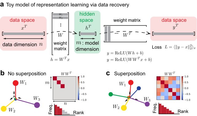
Figure 2: Toy model of superposition. (a) Architecture and loss of the toy model. (b and c) Rows of the weight matrix , denoted by , are representations for features. (b) No superposition represented the most frequent features, i.e., the first three, without interference ( has zero off-diagonal elements). In the frequency-rank plot, height means frequency, and color means . (c) With superposition, more features are represented, while the vectors overlap.
图 2:叠加玩具模型。(a)玩具模型结构与损失。(b 与 c)权矩阵 的行 是特征的表征。(b)无叠加:表示最频繁特征(前三)且无干扰( 非对角为零)。频率–秩图中高度为频率,颜色为 。(c)有叠加时表示更多特征,同时向量 重叠。
To gain understanding of the relationship between superposition and data structure, we need a toy model on learning representation simple enough yet not simpler — two key principles need to be reflected, (i) there are more features to represent than the dimension of the model, and (ii) features occur in data with different frequencies. Later, we will discuss how the loss due to representation studied here may affect the overall final loss in LLMs.
要理解叠加与数据结构的关系,需要一个足够简单却不过度简化的表征学习玩具模型——须体现两条关键原则:(i)待表示特征多于模型维数;(ii)特征在数据中出现频率不等。后文再讨论此处研究的表征损失如何影响 LLM 的总体最终损失。
We adopt the toy model of superposition from Anthropic [26] with minor modifications (Figure 2a). Input data is a vector with data dimension being the number of atomic (or irreducible) features. Each element in is interpreted as the activation of this data point at feature , which is sampled as
我们采用 Anthropic [26] 的叠加玩具模型并略作修改(图 2a)。输入 为向量,数据维 即原子(或不可约)特征数。 中每个元素 解释为该数据点在特征 上的激活,采样为
Here, sampled from a Bernoulli distribution controls whether the feature is activated, and sampled from a uniform distribution controls the activation strength once feature is activated. The frequency of feature to appear in the data is . Without loss of generality, we make the indices of features the same as their frequency or importance rank. The data structure is then about how decreases with rank . The expected number of activations in one data will be referred to as activation density: . The model learns hidden representations by recovering the data, which cannot be done perfectly because the model dimension is much smaller than the number of possible features in the data . The trainable parameters are a weight matrix and a bias vector . The weight matrix embeds data into a hidden space with dimension , , with . In practice, we fix as a large number and change the model dimension . We use to read out the embedding, where . The loss is defined as the difference between the recovered and the original , , where means average over distribution.
其中, 取自伯努利分布,控制特征 是否被激活; 取自均匀分布,控制激活后的强度。特征 在数据中出现的频率为 。不失一般性,令特征下标与其频率或重要性秩相同。数据结构于是关于 如何随秩 下降。一条数据中激活数的期望称为激活密度:。模型通过恢复数据学习隐表征——因模型维 远小于可能特征数 ,无法完美恢复。可训参数为权矩阵 与偏置 。 把数据 嵌入维数为 的隐空间,,且 。实践中固定较大的 ,改变模型维 。用同一 读出嵌入:。损失定义为恢复的 与原 之差,,其中 表示对 分布取平均。
We can now formally introduce superposition. Note that is the representation of feature in the hidden space, where we use to denote the th row of the matrix, in our toy model, feature is well represented when the norm is close to . No superposition ideally means the first rows of form an orthogonal basis (i.e., the first most important features represented perfectly) and the rest of the rows are zero (i.e., rest of the features ignored or lost), as illustrated in Figure 2b. Superposition means that there are more than rows in with norms close to (Figure 2c). Conceptually, superposition is preferred when features are more equal in importance ( are more uniform) and when features are more sparse ( is smaller) [26].
现在可形式引入叠加。注意 是特征 在隐空间中的表征( 为 的第 行);在玩具模型中,当范数 接近 1 时,特征 被良好表示。理想的无叠加意味着: 的前 行构成正交基(前 个最重要特征被完美表示),其余行为零(其余特征被忽略或丢失),如图 2b。叠加则意味着有多于 行的范数接近 1(图 2c)。概念上,当特征重要性更均等( 更均匀)且更稀疏( 更小)时,叠加更受青睐 [26]。
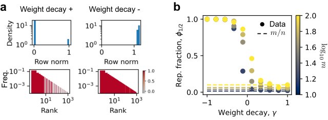
Figure 3: Weight decay can robustly tune the degree of superposition. (a) Given data dimension and feature frequency with , we tested model dimension from to and weight decay from to . The frequency-rank plot shows that important features tend to be represented (color means and colorbar same as Figure 2b). The row norm distribution is bimodal, making a good measure for the fraction represented. Smaller weight decay leads to larger or stronger superposition. (b) After changing , the ability for small weight decay to reach strong superposition is not changed. We show the result at here, more in Appendix D.3.
图 3:权重衰减可稳健调节叠加程度。(a)给定数据维 、特征频率 且 ,测试模型维 从 10 到 100、权重衰减从 到 。频率–秩图显示重要特征倾向于被表示(颜色为 ,色条同图 2b)。行范数分布呈双峰,使 成为已表示比例的良好度量。更小权重衰减对应更大 或更强叠加。(b)改变 后,小权重衰减达到强叠加的能力不变。此处展示 ;更多见附录 D.3。
We found that it is possible to control superposition independently of data properties by modifying the optimizer with a weight decay (or growth) term:
我们发现:通过在优化器中加入权重衰减(或增长)项,可以独立于数据性质控制叠加:
$$W_{i,t+1}=\left{\begin{aligned} &W_{i,t}-\eta_{t}\gamma W_{i,t},\gamma\geq 0,\\gamma<0,\end{aligned}\right. \tag{2}$$
&W_{i,t}-\eta_{t}\gamma W_{i,t}(1/|W_{i,t}|_{2}-1),
where is the learning rate and is the th row of the weight matrix at step (vector operations are element-wise). For weight decay , the update corresponds to gradient descent on , encouraging unit-norm rows. We implement this in a modified AdamW [27] optimizer with a warm-up and cosine decay learning rate schedule. Training runs for 20k–80k steps with batch sizes of 2048–8192, ensuring models reach saturation. At each step, we sample new data using probabilities . We observe that important features are represented as expected, and row norms of become bimodal, clustering near 0 and 1 (Figure 3a). This allows us to define the fraction of represented features as
其中 为学习率, 为第 步权矩阵第 行(向量运算逐元素)。对权重衰减 ,更新对应在 上的梯度下降,鼓励单位范数行。我们在带预热与余弦衰减学习率日程的改动 AdamW [27] 中实现。训练 20k–80k 步,批大小 2048–8192,确保模型达饱和。每步按概率 采样新数据。我们观察到重要特征如预期被表示, 的行范数呈双峰,聚在 0 与 1 附近(图 3a)。于是可定义已表示特征比例为
namely, the fraction of rows with norm larger than . We found that weight decay can tune superposition smoothly, with small weight decay giving strong superposition, i.e., , and large weight decay corresponding to weak superposition, i.e., (Figure 3a). The ability of weight decay to tune superposition is robust to a variety of feature frequency distributions (Figure 3b), where and we control the decay speed of via the data exponent . Thus, weight decay provides a practical knob for controlling superposition in our study.
即范数大于 的行所占比例。我们发现权重衰减可平滑调节叠加:小 给出强叠加,即 ;大权重衰减对应弱叠加,即 (图 3a)。该调节能力对多种特征频率分布稳健(图 3b),其中 ,我们用数据指数 控制 衰减速度。因此,权重衰减为本研究提供了实用的叠加旋钮。
Our toy model differs from LLMs in architecture, data, and loss. Since we focus on representations rather than next-token prediction, we omit transformer layers. Conceptually, LLMs map a document to a token, with inputs and outputs in different spaces, while the toy model operates within a single shared space. Despite this, the toy model captures key aspects of language structure through engineered sparsity and feature importance, making its data structure aligned with that of LLMs at a higher level. While LLMs use cross-entropy loss and the toy model uses squared error, we will show that this does not affect the scaling behavior of the loss. Thus, the toy model is a suitable abstraction for studying representation-limited scaling.
玩具模型在结构、数据与损失上不同于 LLM。因聚焦表征而非下一 token 预测,我们省略 transformer 层。概念上,LLM 把文档映射到 token,输入与输出在不同空间;玩具模型则在单一共享空间内运作。尽管如此,玩具模型通过工程化的稀疏性与特征重要性捕捉语言结构的关键方面,使其数据结构在更高层次与 LLM 对齐。LLM 用交叉熵、玩具模型用平方误差,但我们将表明这不影响损失的缩放行为。因此,玩具模型是研究「表征受限缩放」的合适抽象。
3 Results
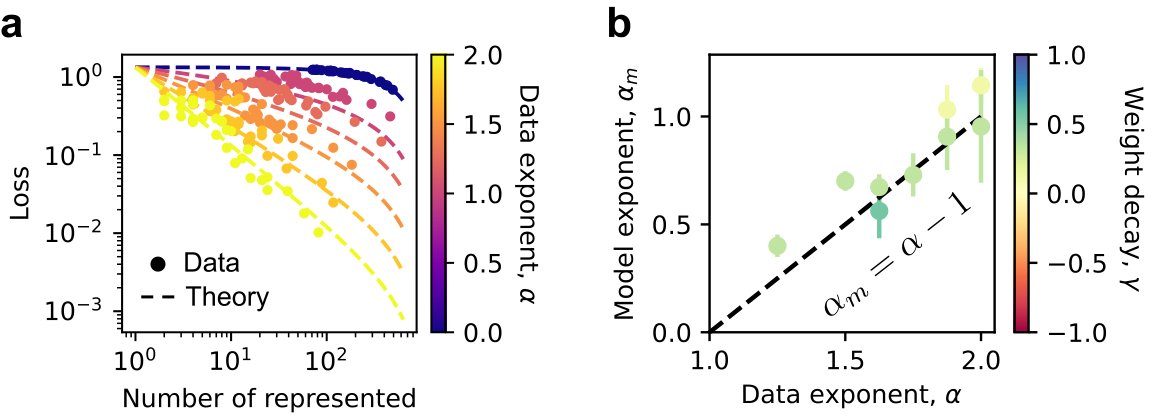
Figure 4: Rich scaling phenomena arise when we change the degree of superposition and data structures. (a) In the same experiments () in Figure 1, where (blue), (yellow), and (green), we use to reach strong superposition and for weak superposition. R-squared value of the fitting is used to measure how likely the fitted part is a power law (Appendix D.4). R-squared values closer to 1 mean that the data are more similar to a power law. We found that at strong superposition, power laws are robust across different underlying feature distributions. Yet, at weak superposition, only power-law feature frequencies can lead to power-law losses. (b) When changing superposition by weight decay and varying feature frequency decay by given , we found roughly three distinct behaviors. For (b), and (more in Appendix D.4).
图 4:改变叠加程度与数据结构时出现丰富缩放现象。(a)与图 1 相同实验(),(蓝)、(黄)、(绿);用 达强叠加、 达弱叠加。用拟合的 R 方度量拟合段有多像幂律(附录 D.4);越接近 1 越像。强叠加下,对不同底层特征分布幂律都稳健;弱叠加下仅幂律特征频率能导致幂律损失。(b)用权重衰减改变叠加、用 改变 的衰减时,大致出现三种不同行为。对(b),,(更多见附录 D.4)。
In the toy model, we found rich phenomena by varying superposition and feature importance. Reviewing the experiments in Figure 1, we set weight decay to have strong superposition and to have weak superposition. We compute squared values from linear fits in log-log plots to quantify scaling behavior, assessing how closely the loss follows a power law to model dimension. We can see that at strong superposition, the losses are close to power laws, regardless of the underlying feature frequencies, yet the loss is a power law at weak superposition if the feature frequency is a power law with rank (Figure 4a). For a systematic scan, we next set and can vary the data exponent to change how fast decays consistently.[^1] Unless otherwise specified, we set activation density as by default, whose value will be shown not to affect the scaling. Assuming a power-law form for the final test loss, , we extract the model exponent from the empirical fit. We fit the loss with a power law in all cases. The fitted reveals how fast losses decay, even in the weak superposition regime where the power law fit is poor (Appendix D.4). Roughly, three distinct patterns emerge: (1) under weak superposition (positive , yellow box in Figure 4b), is small, indicating slow loss decay; (2) under strong superposition and a wide range of small data exponents (red box), remains robustly near 1; (3) for strong superposition with large data exponents (blue box), increases with . By interpreting these three patterns, we aim to understand when loss follows a power law with model dimension, and what determines the exponent when it does.
在玩具模型中,改变叠加与特征重要性可得到丰富现象。回顾图 1 实验:取 为强叠加、 为弱叠加。在双对数图上做线性拟合,用 方量化缩放行为,评估损失相对模型维有多接近幂律。可见强叠加下损失接近幂律,不论底层特征频率如何;弱叠加下仅当 随秩 呈幂律时损失才是幂律(图 4a)。系统扫描中,接着取 ,用数据指数 一致改变 衰减速度。[^1] 除非另说明,默认激活密度 ,其取值后文将表明不影响缩放。假设最终测试损失呈幂律 ,从经验拟合提取模型指数 。所有情形都用幂律拟合损失;即便弱叠加区幂律拟合较差, 仍揭示损失衰减快慢(附录 D.4)。大致出现三种模式:(1)弱叠加(正 ,图 4b 黄框)下 小,损失衰减慢;(2)强叠加且数据指数在较宽的小范围内(红框), 稳健地接近 1;(3)强叠加且数据指数大(蓝框)时, 随 增大。通过解读这三种模式,我们试图理解:损失何时相对模型维呈幂律,以及呈幂律时指数由什么决定。
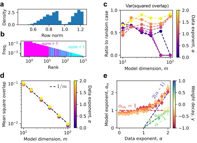
Figure 5: Loss at weak superposition can be well described by the expected number of activated but unlearned features. (a) The actual loss and theory at weak superposition (Equation (4)) agree when weight decay is positive. (b) For those closest to the ideal no superposition case (Appendix D.5), we expect , which is close to measured values. Error bars are standard errors.
图 5:弱叠加下的损失可由「被激活但未学习」特征的期望数很好描述。(a)弱叠加下实际损失与理论(式 (4))在权重衰减为正时吻合。(b)对最接近理想无叠加的情形(附录 D.5),期望 ,与测得值接近。误差棒为标准误。
We begin by analyzing the weak superposition regime. Consider an idealized case where the top most frequent features are perfectly represented, where is the fraction of represented features. The loss can then be written as:
我们先分析弱叠加区。考虑理想情形:最频繁的前 个特征被完美表示, 为已表示特征比例。损失可写为:
The first equality follows from the definition of loss. The second holds because the first features are assumed to be perfectly reconstructed, and the remaining features are ignored (i.e., for ). The final expression uses the definition of , where , giving . To approximate the remaining sum, we use the integral and refer to this estimate as the loss by unlearned features. We find that, in the weak superposition regime, the actual losses closely match this prediction (Figure 5a). Slight discrepancies — where actual losses are slightly higher — can be attributed to the fact that models do not exactly learn the first features. In contrast, in the strong superposition regime, the predicted loss by unlearned features is nearly zero, yet the actual loss remains non-zero, indicating additional sources of error. Focusing on cases closest to the ideal no-superposition scenario — where and the first features are represented — we observe that such cases occur when and yield a model exponent (Figure 5b). This matches the theoretical expectation that when and . Thus, in the weak superposition regime, loss scaling is well described by the contribution of unlearned features, that is, the total frequency of features not represented by the model.
第一个等号来自损失定义。第二个成立是因为假定前 个特征被完美重建,其余被忽略(即 时 )。最终表达式用 ,且 ,故 。对其余和用积分 逼近,称此估计为「未学习特征带来的损失」。我们发现弱叠加下实际损失与该预测密切吻合(图 5a)。略高的微小偏差可归因于模型并非精确学会前 个特征。相反,强叠加下按未学习特征预测的损失近乎为零,实际损失仍非零,说明还有其他误差来源。聚焦最接近理想无叠加—— 且前 个特征被表示——的情形,我们观察到它们出现在 时,并给出模型指数 (图 5b)。这与理论期望一致:当 且 时,。因此弱叠加区的损失缩放,可由未学习特征的贡献——即模型未表示特征的总频率——很好描述。
We can now explain when loss follows a power law in the weak superposition regime. When feature frequencies follow a power law, with , the integral becomes a power law in . And if the scales approximately as a power of model size (ideally it is ). Then the loss also scales as a power law in . Consequently, the deviations from power-law behavior seen in Figure 1b — for non-power-law — are consistent with this explanation. Moreover, when with , we expect the model exponent to be , which matches the relatively small values of observed on the right side of Figure 4b. In summary, the weak superposition regime reveals a strong dependence of loss vs. model dimension scaling on the structure of feature frequencies in the data.
现在可解释弱叠加下损失何时呈幂律。当特征频率服从幂律 且 时,积分 成为 的幂律;若 又近似随模型规模 呈幂(理想为 ),则损失也随 呈幂律。因此图 1b 中非幂律 偏离幂律的行为与此解释一致。此外,当 且 时,期望模型指数 ,与图 4b 右侧相对较小的 吻合。总之,弱叠加区显示:损失相对模型维的缩放强烈依赖数据中特征频率的结构。
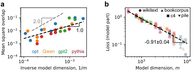
Figure 6: Loss scaling at strong superposition is mainly explained via geometry. (a) The more frequent the features are, the more likely their norms are greater than (purple). (b) The row norm distribution is bimodal around . Related results can be found in Appendix D.6. (c) Fraction of strongly represented features () at stong superposition () is around (fast increasing dashed line), which is much larger than (slowly increasing dashed line). (d) The strongly represented features have decreasing overlaps as expected, where we plotted all the data when , and the dashed line is . (e) At strong superposition, (horizontal line) if the strongly represented features having small overlaps dominate, which is true for a wide range of . But (fast increasing dashed line) if weakly represented ones with large overlaps dominate, explaining the measured when is large. Error bars are standard errors.
图 6:强叠加下的损失缩放主要由几何解释。(a)特征越频繁,其范数越可能大于 (紫)。(b)行范数分布在 附近呈双峰。相关结果见附录 D.6。(c)强叠加()下强表示特征比例()约在 (快速上升虚线),远大于 (缓慢上升虚线)。(d)强表示特征的重叠如预期下降;图中画出 的全部数据,虚线为 。(e)强叠加下,若小重叠的强表示特征占主导,则 (水平线)——这对较宽的 范围成立;若大重叠的弱表示特征占主导,则 (快速上升虚线),解释 较大时测得的 。误差棒为标准误。
We now turn to the strong superposition regime, where all features are represented. In this regime, the loss arises primarily from the non-zero overlaps between representation vectors. For instance, consider the case where only feature is activated in the data. Even for , the output receives contributions on the order of , leading to a loss that scales as due to the squared error objective. The nonlinearity nonlinearity and bias terms do not affect the scaling behavior (Appendix A.1). Consequently, we study the overlaps between representation vectors when the number of vectors exceeds the dimensionality of the space.
现在转向强叠加区——所有特征都被表示。此区间损失主要来自表征向量间非零重叠。例如数据中仅特征 被激活时,即便 ,输出 也会收到量级为 的贡献,平方误差目标下损失按 缩放。 非线性与偏置项不影响缩放行为(附录 A.1)。因此,我们在向量数超过空间维数时研究表征向量间的重叠。
We now provide theoretical expectations for vector overlaps. Consider unit vectors with . It can be shown that [28]
下面给出向量重叠的理论期望。考虑 个单位向量 且 。可以证明 [28]
This lower bound, , approaches when . The bound is met when the vectors form an equal angle tight frame (ETF) [29, 30, 31], which minimizes interference and appears in contexts such as quantum measurements [32, 33, 34, 35] and neural collapse [36, 37]. However, ETFs in real space can only exist if [29, 30, 31]. In our toy model, feature frequencies vary, so exact equal-angle configurations are suboptimal — important features may benefit from smaller overlaps. Nonetheless, when feature frequencies are nearly uniform (e.g., small data exponent ), remains a good estimate. Although the rows are not strictly unit vectors, they are close enough that the scaling behavior remains valid. In summary, we expect that in the strong superposition regime: (i) Many representation vectors can approximate a mutually orthogonal configuration, with typical overlaps scaling as ; (ii) The number of such vectors can be much larger than but still bounded (e.g., for ETFs), so when is too large, some feature vectors cannot be in such configurations, having larger overlaps.
该下界 在 时趋近 。当向量构成等角紧框架(ETF)[29, 30, 31] 时达到该界——ETF 最小化干扰,并出现在量子测量 [32, 33, 34, 35] 与神经坍缩 [36, 37] 等语境。但实空间中 ETF 仅当 时可能存在 [29, 30, 31]。玩具模型中特征频率不等,精确等角配置并非最优——重要特征或受益于更小重叠。尽管如此,当特征频率近乎均匀(例如数据指数 小)时, 仍是良好估计。虽行 并非严格单位向量,但足够接近,缩放行为仍成立。总之,强叠加区我们期望:(i)许多表征向量可近似相互正交配置,典型重叠按 缩放;(ii)此类向量数可远大于 但仍有界(例如 ETF 约 ),故当 过大时,部分特征向量无法处于此类配置,重叠更大。
With these theoretical expectations in hand, we evaluate our trained toy models. The first step is to test for the presence of a nearly orthogonal configuration among representation vectors. A preliminary clue comes from examining the norms of the rows , which exhibit a bimodal distribution: one peak slightly below 1, corresponding to less frequent features, and another above 1, corresponding to the most frequent ones (Figure 6, a and b). This suggests that the most important features are represented in a nearly orthogonal manner, while less important ones exhibit greater overlap. To quantify this, we compute the fraction of rows with norm exceeding 1:
有了这些理论期望,我们评估已训玩具模型。第一步检验表征向量中是否存在近正交配置。初步线索来自行 的范数:呈双峰分布——一峰略低于 1,对应较少频特征;另一峰高于 1,对应最频繁特征(图 6a、b)。这表明最重要特征以近正交方式表示,较不重要者重叠更大。为量化,我们计算范数超过 1 的行所占比例:
which significantly exceeds and is around the ETF expectation (Figure 6c). For these rows, the mean squared overlaps match the theoretical bound well (Figure 6d). Although these vectors do not form a perfect ETF, their configuration is much closer to an ETF than random initialization (Appendix D.6). In contrast, rows with norms less than exhibit larger overlaps on average (Appendix D.6). We refer to rows with as strongly represented features and those with smaller norms as weakly represented. These results confirm our expectations: strongly represented features attempt to form an approximately orthogonal configuration with typical overlaps scaling as ; their number exceeds a lot but remains bounded, necessitating the presence of weakly represented features with larger overlaps.
该比例显著超过 ,并接近 ETF 期望 (图 6c)。对这些行,平均重叠平方与理论界 吻合良好(图 6d)。虽非完美 ETF,其配置远比随机初始化更接近 ETF(附录 D.6)。相反,范数小于 的行平均重叠更大(附录 D.6)。我们称 的行为强表示特征,范数更小的为弱表示。结果确认期望:强表示特征试图形成典型重叠按 缩放的近似正交配置;其数量远超 但仍有界,因而必然存在重叠更大的弱表示特征。
Figure 7: Activation density does not affect scaling exponents in our tests. (a) Loss is roughly proportional to activation density given the degree of superposition (, ). (b) So, will only affect the coefficient but not the exponent when considering the power law with model dimension. We plot the evidence at strong superposition, see more in Appendix D.7.
图 7:激活密度在我们的测试中不影响缩放指数。(a)给定叠加程度时,损失大致与激活密度成正比(,)。(b)因此考虑相对模型维的幂律时, 只影响系数不影响指数。我们画出强叠加下 的证据;更多见附录 D.7。
In the strong superposition regime, the loss is mainly determined by a weighted sum of squared overlaps between representation vectors. For strongly represented features, where overlaps scale as , the loss contribution scales as . In contrast, weakly represented features can have large, constant overlaps. In the worst case, their total contribution is proportional to , where we approximate . (See Appendix A.1 for loss decomposition details) If the loss is dominated by the strongly represented features, we expect the overall loss to scale as . In the opposite limit — when weakly represented features dominate — the loss scales as , meaning the effective model exponent becomes . Although we do not solve the toy model analytically, we hypothesize that as increases (i.e., feature frequencies become more skewed), optimization prioritizes minimizing the loss of the most frequent features. As a result, the remaining loss is mostly due to the weakly represented ones. Empirically, we find a simple and elegant rule (Figure 6e):
强叠加区损失主要由表征向量间重叠平方的加权和决定。对强表示特征,重叠按 缩放,损失贡献按 缩放。弱表示特征则可有大的常值重叠;最坏情形下其总贡献正比于 ,其中近似 。(损失分解细节见附录 A.1)若损失由强表示特征主导,期望总体损失按 缩放;相反若弱表示主导,损失按 缩放,有效模型指数变为 。虽未解析求解玩具模型,我们假设:随 增大(特征频率更偏斜),优化优先最小化最频繁特征的损失,剩余损失主要来自弱表示者。经验上我们找到一条简单优雅的规则(图 6e):
In short, the optimization selects whether strongly or weakly represented features dominate the loss, whichever leads to faster decay with model size . We now have a full picture that the origin of lies in the geometric constraints on vector overlaps, and this scaling is robust as long as the feature frequency distribution is not too skewed.
简言之,优化选择让强表示或弱表示特征主导损失——取随模型规模 衰减更快的那一方。至此全貌清楚: 的起源在于向量重叠的几何约束,只要特征频率分布不太偏斜,该缩放就稳健。
We also studied the effect of the number of expected activated features or activation density , which was set to . By fixing data exponent , which will be shown to be relevant to natural language, we can scan different superposition degrees and activation densities. Since is required, which is equivalent to , we have , setting the upper bound for our scanning. We found that loss is approximately proportional to activation density (Figure 7a). This fact suggests that the power law exponent should not change, which we confirmed (Figure 7b). Under a controlled superposition degree, activation density linearly increases loss and thus does not affect the scaling exponents in our experiments.
我们还研究了期望激活特征数即激活密度 的影响,此前设为 。固定数据指数 (后文将表明与自然语言相关),可扫描不同叠加程度与激活密度。因要求 (等价于 ),有 ,构成扫描上界。我们发现损失近似与激活密度 成正比(图 7a),暗示幂律指数不应改变——已确认(图 7b)。在受控叠加程度下,激活密度线性抬高损失,因而不影响我们实验中的缩放指数。
Figure 8: Superposition may explain the neural scaling law observed in actual LLMs. We evaluate four open-sourced model classes, Opt [38], GPT2 [39], Qwen [40], and Pythia [41], which have model sizes from around 100M to 70B (details in Appendix C). (a) We found the mean square overlaps of roughly follow scaling, where is the language model head. (b) The model class is reflected by color as panel a, while we use shapes for evaluation datasets [42, 43, 44, 45]. The loss related to model size is fitted as a power law, yielding empirical close to (details in Appendix D.8).
图 8:叠加或可解释真实 LLM 中观测到的神经缩放律。我们评估四个开源模型类:Opt [38]、GPT2 [39]、Qwen [40] 与 Pythia [41],规模约从 100M 到 70B(细节见附录 C)。(a)发现 的均方重叠大致服从 缩放,其中 为语言模型头。(b)模型类用与面板 a 相同的颜色,评估数据集 [42, 43, 44, 45] 用形状。与模型规模相关的损失按幂律拟合,得经验 ,接近 (细节见附录 D.8)。
Finally, we explore how the phenomena found in our toy model might be relevant to real LLMs [38, 39, 40, 41]. As a simple mapping, we treat tokens as atomic features, with data dimension equal to the vocabulary size. The model dimension for LLMs is known. We analyze the language model head, denoted by the weight matrix . Through the norm and interference distributions of the rows of , we claim LLMs are in superposition (Appendix D.8). If we measure token frequency, it follows a power law with exponent close to (Appendix D.8). We conclude, based on the knowledge from toy models, that LLMs operate in a superposition regime, and expect loss to be dominated by small overlaps of the strongly represented . We next calculated the mean squared overlaps of normalized rows , and found they roughly obey scaling (Figure 8a). We argue that cross-entropy loss, given that the overlaps are small in absolute value, can be expanded and approximately scales as the mean square overlaps (Appendix A.2). We therefore expect the loss of representation-limited LLMs to have scaling. LLM losses are close to a linear function of (Appendix D.8). Yet when , the extrapolation of losses does not hit . The non-zero intersection can be due to intrinsic uncertainty in language. Increasing model sizes decreases “wrong" interferences but cannot eliminate uncertainty in the data. So, as in previous papers where loss is decomposed into model size part, dataset size part, and a constant [3], we fit our loss values by the following,
最后,我们探索玩具模型中的现象如何与真实 LLM 相关 [38, 39, 40, 41]。简单映射下,把 token 当作原子特征,数据维 等于词表大小;LLM 的模型维 已知。我们分析语言模型头权矩阵 。通过 行的范数与干扰分布,我们主张 LLM 处于叠加(附录 D.8)。若度量 token 频率,它服从指数 接近 的幂律(附录 D.8)。基于玩具模型知识,我们结论:LLM 在叠加区运行,并期望损失由强表示者的小重叠 主导。接着计算归一化行 的均方重叠,发现大致服从 缩放(图 8a)。我们论证:在重叠绝对值较小时,交叉熵可展开并近似按均方重叠缩放(附录 A.2)。因此期望表征受限 LLM 的损失具有 缩放。LLM 损失接近 的线性函数(附录 D.8);但当 时,外推并不过零。非零截距可来自语言内在不确定性——增大模型减小「错误」干扰,却无法消除数据中的不确定性。故如先前把损失分解为模型规模部分、数据集规模部分与常数 [3],我们按下式拟合损失:
where the model size part is universal (model size is a function of ), and contains loss irrelevant to model size, depending on the evaluation dataset and model class. The fitting yields (Figure 8b). We inferred from the Chinchilla models [3] that due to model size (Appendix D.8), , where [46] is the power-law exponent of loss with model size. The exponents from LLMs are close to 1.
其中模型规模部分 具有普适性(模型规模是 的函数), 含与模型规模无关的损失,依赖评估数据集与模型类。拟合得 (图 8b)。从 Chinchilla 模型 [3] 推断:因模型规模 (附录 D.8),,其中 [46] 为损失随模型规模的幂律指数。LLM 的 均接近 1。
In conclusion, we presented a comprehensive picture through the toy model, at different superposition degrees and data structures, of when the loss scales as a power law with model dimension or size, and what governs the scaling exponent. We confirmed that LLMs operate in the strong superposition regime. Moreover, LLMs [38, 39, 40, 41] quantitatively match toy model predictions: the model exponent is close to , and representation overlap scales as . The inferred exponent for Chinchilla models [3] is also close to 1. Superposition is therefore an important mechanism underlying the observed scaling laws.
总之,我们通过玩具模型在不同叠加程度与数据结构下给出全景:损失何时随模型维或规模呈幂律,以及缩放指数由什么决定。我们确认 LLM 处于强叠加区;且 LLM [38, 39, 40, 41] 与玩具模型预测定量吻合:模型指数 接近 ,表征重叠按 缩放。从 Chinchilla 模型 [3] 推断的 也接近 1。因此叠加是观测到的缩放律背后的重要机制。
4 Related works
Neural scaling laws were first characterized empirically [2], demonstrating that for LLMs, the cross-entropy loss improves predictably as a power-law with increased model size (parameters), dataset size, or compute, over multiple orders of magnitude. This finding is built on earlier observations (e.g. [47]) that deep learning performance scales in a smooth power-law fashion with data and model growth. Key works showed the surprisingly universal nature of such scaling behaviors across architectures and tasks [2, 3, 4], directing further development of LLMs.
神经缩放律首先被经验刻画 [2]:对 LLM,交叉熵损失随模型规模(参数)、数据集规模或算力增大,在多个数量级上可预测地按幂律改善。该发现建立在更早观察之上(如 [47]):深度学习表现随数据与模型增长呈平滑幂律。关键工作展示了此类缩放行为跨架构与任务的惊人普适性 [2, 3, 4],并指引了 LLM 的进一步发展。
Several heuristic toy models have been proposed to explain neural scaling laws. One common view is that models aim to fit data manifolds or functions, and the scaling exponents depend strongly on the structure of the data [14, 15]. Another group of models assumes the network learns discrete features or skills [18, 19], whose importance follows a power-law distribution, giving results the same as ours in the weak superposition regime. One toy model predicts that loss scales inversely with model width [24], arguing that parameters independently perform the same task with noise, and the scaling follows from the central limit theorem. However, this model applies mainly in the overparameterized regime.
若干启发式玩具模型被提出以解释神经缩放律。一种常见观点是模型旨在拟合数据流形或函数,缩放指数强烈依赖数据结构 [14, 15]。另一组模型假定网络学习离散特征或技能 [18, 19],其重要性服从幂律分布,结果与我们在弱叠加区相同。有玩具模型预测损失与模型宽度成反比 [24],论证参数独立完成同一任务并带噪声,缩放来自中心极限定理;但该模型主要适用于过参数化区间。
More formal approaches from statistical learning theory still rely on similar heuristics. The scaling behavior depends on how the limits of dataset size and model size are taken. When the dataset is fixed and model size grows to infinity, the system is variance-limited, and loss scales as by central limit theorem arguments [15]. When the dataset size grows to infinity first, the loss scaling enters the resolution-limited regime. In kernel methods, this leads to [15, 16, 17], consistent with our weak superposition regime. Here, is the exponent of the power-law decay of kernel eigenvalues, which can be interpreted as abstract feature importance. This regime has also been described as fitting the data manifold [15]. Thus, previous studies mainly address weak superposition or overfitting regimes, while our work reveals new behaviors in the underfitting (where the number of features far exceeds the model dimension) and strong superposition regime, which might be more relevant to LLMs.
统计学习理论中更形式的方法仍依赖类似启发式。缩放行为取决于如何取数据集规模与模型规模的极限。当数据集固定、模型规模趋于无穷时,系统方差受限,由中心极限定理损失按 缩放 [15]。当数据集规模先趋于无穷,损失进入分辨率受限区间。在核方法中,这导致 [15, 16, 17],与我们的弱叠加区一致;此处 是核特征值幂律衰减的指数,可解释为抽象特征重要性。该区间也被描述为拟合数据流形 [15]。因此先前研究主要处理弱叠加或过拟合区间,而我们的工作揭示了欠拟合(特征数远超模型维)与强叠加区的新行为——这可能与 LLM 更相关。
Our toy model is Anthropic’s model of superposition [26], with changes in data sampling. The original study explored how data structure influences superposition but did not explicitly control it. Related models have appeared in compressed sensing [48, 49, 50, 51] and neural information processing [52, 53], though key differences arise due to distinct contexts and objectives.
我们的玩具模型是 Anthropic 的叠加模型 [26],数据采样有改动。原研究探索了数据结构如何影响叠加,但未显式控制叠加。相关模型亦出现在压缩感知 [48, 49, 50, 51] 与神经信息处理 [52, 53] 中,但因语境与目标不同而有关键差异。
5 Discussion
We acknowledge that our work is built on observations of the toy model and shallow theoretical analysis without rigorously solving the toy model. We are thus limited to explaining some deeper questions. For example, Equation (7) is an observation. Although we explained the two extremes, and , and provided heuristics for a transition, we cannot predict the exact transition.
我们承认工作建立在玩具模型观察与浅层理论分析之上,并未严格求解玩具模型,因而对某些更深层问题解释有限。例如式 (7) 是观察结果:虽解释了 与 两个极端并给出过渡启发式,但无法预测精确过渡点。
Neural scaling laws also include scaling laws with dataset size and with training steps, which we did not study. At each step, a fixed number of new data are used for optimization. So, we expect the scaling with the total data amount and that with training steps will be the same, similar to the results at weak superposition [19]. However, in the strong superposition regime, data or training step scaling is related to angle distribution and how angles between representations evolve, which cannot be easily explained without rigorous solving. Future works with better theoretical analysis of our toy model are needed to answer these detailed or extended questions.
神经缩放律还包括随数据集规模与训练步数的缩放,本文未研究。每步用固定数量的新数据做优化,故期望随总数据量与随训练步数的缩放相同,类似弱叠加下的结果 [19]。但在强叠加区,数据或训练步缩放与角度分布以及表征间角度如何演化相关,不经严格求解不易解释。需要未来对玩具模型做更好理论分析,以回答这些细节或扩展问题。
Our analysis suggests LLMs are in the strong superposition regime, but the underlying reasons were not studied. Specifically, LLMs do not need weight growth to have strong superposition. The use of cross-entropy loss or softmax function may be important — minimizing the interference from an unimportant token prefers to make the representation non-zero with negative overlaps with others. Another contributing factor may be that in LLMs, which could make it easier for a nearly mutually orthogonal configuration to form, thereby favoring superposition.
我们的分析表明 LLM 处于强叠加区,但底层原因未研究。具体地,LLM 无需权重增长 即可有强叠加。交叉熵损失或 softmax 函数可能重要——最小化来自不重要 token 的干扰时,偏好让表征非零且与其他表征负重叠。另一可能因素是 LLM 中 ,更易形成近相互正交配置,从而青睐叠加。
We focused on representation loss in this study, yet LLMs should also have losses due to parsing or processing in the transformer layers. As a conceptual discussion, we imagine that the loss associated with model size can be written as
本研究聚焦表征损失,但 LLM 还应有 transformer 层中解析或处理带来的损失。作为概念讨论,我们设想与模型规模相关的损失可写为
where is the depth of the LLM, and are two functions capturing the loss due to representation and parsing, respectively. We can write the equality because depends on in LLMs [38, 39, 40, 41]. Given model size , and are constrained (roughly, ). There is an optimal - relationship such that the loss can be minimized given [54]. At this optimal - relationship, and should be balanced. One can see that the empirical - relationship is not optimal according to [54] but is close. Therefore, following such - relation, we expect to be similar to . And if due to superposition and is similar, we can measure an empirical from data, which is true. So, we conclude that superposition is an important mechanism underlying the loss and scaling laws we see. However, since we do not know the function , we cannot predict the optimal - relation or the exponent .
其中 为 LLM 深度, 与 分别刻画表征与解析带来的损失。可写成等式是因为 LLM 中 依赖 [38, 39, 40, 41]。给定模型规模 , 与 受约束(大致 )。存在最优 – 关系,使给定 时损失 可最小化 [54]。在该最优关系上, 与 应平衡。可见经验 – 关系按 [54] 并非最优但接近。因此沿该关系,期望 与 相似;若因叠加有 且 类似,则可从数据测得经验 ——事实如此。故我们结论叠加是所见损失与缩放律背后的重要机制。但因不知函数 ,无法预测最优 – 关系或指数 。
A natural future direction is to study the parsing-limited scaling (i.e, function). We hypothesize that parsing-limited scaling may resemble the scaling behavior observed when fitting functions or manifolds. The open-source LLMs we examined, as well as those studied in prior neural scaling law papers [2, 3], span model sizes from 100M to 70B parameters, where width (model dimension) varies. However, in the regime from 70B to 700B [38, 39, 40, 41], model scaling seems to focus on increasing depth. We therefore expect parsing-limited scaling to become important for models larger than 70B. It is also plausible that the observed scaling of inference time [55] is connected to this parsing-limited regime. The study of neural scaling laws can be refined by distinguishing between width-limited and depth-limited regimes. In each regime, there should be loss decay behaviors with model size, dataset size, and training steps, highlighting the need for further investigation.
自然的未来方向是研究解析受限缩放(即 函数)。我们假设解析受限缩放可能类似拟合函数或流形时观测到的缩放。我们所检开源 LLM 以及先前神经缩放律论文 [2, 3] 中的模型,规模从 100M 到 70B,宽度(模型维)在变;而在 70B 到 700B 区间 [38, 39, 40, 41],模型缩放似乎聚焦加深。因此期望解析受限缩放对大于 70B 的模型变得重要。观测到的推理时间缩放 [55] 也可能与该解析受限区间相关。神经缩放律研究可通过区分宽度受限与深度受限区间来细化;每个区间都应有随模型规模、数据集规模与训练步数的损失衰减行为,凸显进一步研究的必要。
Beyond explaining existing phenomena, our results may offer guidance for future LLM development and training strategies. If our framework accounts for the observed neural scaling laws [3], we suggest that this kind of scaling is reaching its limits — not because increasing model dimension is impossible, but because it is inefficient. Recognizing that superposition benefits LLMs, we propose that encouraging superposition could enable smaller models to match the performance of larger ones and make training more efficient. Recent architectures such as nGPT [56], which constrain hidden states and weight matrix rows to lie on the unit sphere, demonstrate improved performance and faster training. We interpret these methods as analogous to our weight growth mechanism, both of which promote superposition. Conversely, weight decay is expected to suppress superposition. Prior work has shown that weight decay in LLMs is used primarily for training stability rather than performance gains. Alternative optimization techniques that stabilize training without weight decay have shown promising results [57], potentially due to enhanced superposition. In summary, promoting strong superposition may be a fruitful direction for the design of both LLM architectures and optimization algorithms.
除解释既有现象外,结果或可为未来 LLM 发展与训练策略提供指引。若我们的框架解释了观测到的神经缩放律 [3],我们建议这类缩放正接近极限——并非不能再增大模型维,而是效率低下。认识到叠加有利于 LLM,我们提议鼓励叠加或可使更小模型匹配更大模型的表现,并使训练更高效。近期如 nGPT [56] 等架构把隐状态与权矩阵行约束在单位球上,展示更好表现与更快训练;我们将其解读为类似我们的权重增长机制,二者都促进叠加。相反,权重衰减预期抑制叠加。先前工作显示 LLM 中权重衰减主要用于训练稳定而非性能增益;不靠权重衰减也能稳定训练的替代优化技术已有有希望结果 [57],或因增强了叠加。总之,促进强叠加或是设计 LLM 架构与优化算法的有益方向。
As a side note, while pre-training loss is a key indicator of model performance, it should not be the sole metric of interest. At the same loss level, LLMs with different degrees of superposition may exhibit differences in emergent abilities such as reasoning or trainability via reinforcement learning [58]. Understanding these differences is an important direction for future research.
附带一提:预训练损失虽是模型表现的关键指标,不应是唯一关注度量。在相同损失水平下,叠加程度不同的 LLM 在推理或经强化学习可训性等涌现能力上或有差异 [58]。理解这些差异是重要未来方向。
In conclusion, we demonstrated that superposition of representations can give rise to fast power law decay of loss with model size — a phenomenon that holds across a wide range of data structures and may help explain the neural scaling laws observed in LLMs [3]. Our results contribute to a deeper understanding of modern artificial intelligence systems. This work also opens rich directions for future research. We hope our insights will support the continued development and training of more capable and efficient LLMs.
总之,我们展示表征叠加可带来损失随模型规模的快速幂律衰减——该现象在广泛数据结构上成立,或有助于解释 LLM 中观测到的神经缩放律 [3]。结果加深对现代人工智能系统的理解,并开辟丰富未来研究方向。希望这些洞见支持继续发展与训练更强、更高效的 LLM。
References
[1] Tom B Brown, Benjamin Mann, Nick Ryder, Melanie Subbiah, Jared Kaplan, Prafulla Dhariwal, Arvind Neelakantan, et al. Language models are few-shot learners. Advances in Neural Information Processing Systems , 33:1877–1901, 2020.
[2] Jared Kaplan, Sam McCandlish, Tom Henighan, Tom B Brown, Benjamin Chess, Rewon Child, Scott Gray, Alec Radford, Jeffrey Wu, and Dario Amodei. Scaling laws for neural language models. arXiv preprint arXiv:2001.08361 , 2020.
[3] Jordan Hoffmann, Sebastian Borgeaud, Arthur Mensch, Jack W Rae, Alana Lai, Joel Wang, Katie Millican, Susannah Young, Olivier Tieleman, et al. Training compute-optimal large language models. arXiv preprint arXiv:2203.15556 , 2022.
[4] Tom Henighan, Jared Kaplan, Mor Katz, Mark Chen, Christopher Hesse, Jacob Jackson, Heewoo Jun, Tom B. Brown, Prafulla Dhariwal, Scott Gray, Chris Hallacy, Benjamin Mann, Alec Radford, Aditya Ramesh, Nick Ryder, Daniel M. Ziegler, John Schulman, Dario Amodei, and Sam McCandlish. Scaling laws for autoregressive generative modeling, 2020.
[5] OpenAI. Gpt-4 technical report, 2023. https://openai.com/research/gpt-4.
[6] Haotong Qin, Ge-Peng Ji, Salman Khan, Deng-Ping Fan, Fahad Shahbaz Khan, and Luc Van Gool. How good is google bard’s visual understanding? an empirical study on open challenges. arXiv preprint arXiv:2307.15016 , 2023. https://arxiv.org/abs/2307.15016.
[7] Aitor Lewkowycz, Pasquale Minervini, Jacob Andreas, et al. Solving quantitative reasoning problems with language models. arXiv preprint arXiv:2206.14858 , 2022. https://arxiv.org/abs/2206.14858.
[8] Ross Taylor, Marcin Kardas, Guillem Cucurull, Thomas Scialom, Andrew Hartshorn, Elvis Saravia, Andrew Poulton, et al. Galactica: A large language model for science. arXiv preprint arXiv:2211.09085 , 2022. https://arxiv.org/abs/2211.09085.
[9] Stephen Wolfram. Wolfram|alpha as the computation engine for gpt models, 2023. https://www.wolfram.com/wolfram-alpha-openai-plugin.
[10] Trieu H. Trinh, Yuhuai Wu, Quoc V. Le, He He, and Thang Luong. Solving olympiad geometry without human demonstrations. Nature , 2024. https://www.nature.com/articles/s41586-024-00001-2.
[11] Mark Chen, Jerry Tworek, Heewoo Jun, Qiming Yuan, et al. Evaluating large language models trained on code. arXiv preprint arXiv:2107.03374 , 2021. https://arxiv.org/abs/2107.03374.
[12] GitHub. Github copilot: Your ai pair programmer, 2022. https://github.com/features/copilot.
[13] Jack W Rae, Sebastian Borgeaud, Trevor Cai, et al. Scaling language models: Methods, analysis & insights from training gopher. arXiv preprint arXiv:2112.11446 , 2021. https://arxiv.org/abs/2112.11446.
[14] Utkarsh Sharma and Jared Kaplan. Neural scaling laws: A low-dimensional perspective. Journal of Machine Learning Research , 23(228):1–29, 2022.
[15] Yasaman Bahri, Ethan Dyer, Jared Kaplan, Jaehoon Lee, and Utkarsh Sharma. Explaining neural scaling laws. Proceedings of the National Academy of Sciences , 121(27):e2311878121, 2024.
[16] Blake Bordelon, Abdulkadir Canatar, and Cengiz Pehlevan. Spectrum dependent learning curves in kernel regression and wide neural networks. In International Conference on Machine Learning , pages 1024–1034. PMLR, 2020.
[17] Alexander Maloney, Daniel A Roberts, and James Sully. A solvable model of neural scaling laws. arXiv preprint arXiv:2210.16859 , 2022.
[18] Marcus Hutter. Learning curve theory. arXiv preprint arXiv:2102.04074 , 2021.
[19] Eric Michaud, Ziming Liu, Uzay Girit, and Max Tegmark. The quantization model of neural scaling. Advances in Neural Information Processing Systems , 36:28699–28722, 2023.
[20] Ziming Liu, Yizhou Liu, Eric J Michaud, Jeff Gore, and Max Tegmark. Physics of skill learning. arXiv preprint arXiv:2501.12391 , 2025.
[21] Danny Hernandez, Tom Brown, Tom Conerly, Nova DasSarma, Dawn Drain, Sheer El-Showk, Nelson Elhage, Zac Hatfield-Dodds, Tom Henighan, Tristan Hume, et al. Scaling laws and interpretability of learning from repeated data. arXiv preprint arXiv:2205.10487 , 2022.
[22] Ari Brill. Neural scaling laws rooted in the data distribution. arXiv preprint arXiv:2412.07942 , 2024.
[23] Stefano Spigler, Mario Geiger, and Matthieu Wyart. Asymptotic learning curves of kernel methods: empirical data versus teacher–student paradigm. Journal of Statistical Mechanics: Theory and Experiment , 2020(12):124001, 2020.
[24] Jinyeop Song, Ziming Liu, Max Tegmark, and Jeff Gore. A resource model for neural scaling law, 2024.
[25] Sanjeev Arora, Yuanzhi Li, Yingyu Liang, Tengyu Ma, and Andrej Risteski. Linear algebraic structure of word senses, with applications to polysemy, 2018.
[26] Nelson Elhage, Tristan Hume, Catherine Olsson, Nicholas Schiefer, Tom Henighan, Shauna Kravec, Zac Hatfield-Dodds, Robert Lasenby, Dawn Drain, Carol Chen, Roger Grosse, Sam McCandlish, Jared Kaplan, Dario Amodei, Martin Wattenberg, and Christopher Olah. Toy models of superposition. Transformer Circuits Thread , 2022.
[27] Ilya Loshchilov and Frank Hutter. Decoupled weight decay regularization. In International Conference on Learning Representations , 2019.
[28] L. Welch. Lower bounds on the maximum cross correlation of signals. IEEE Transactions on Information Theory , 20(3):397–399, 1974.
[29] Peter G Casazza and Gitta Kutyniok. Finite frames: Theory and applications . Springer Science & Business Media, 2012.
[30] Thomas Strohmer and Robert W Heath. Grassmannian frames with applications to coding and communication. Applied and Computational Harmonic Analysis , 14(3):257–275, 2003.
[31] Matthew Fickus, Dustin G Mixon, and Janet C Tremain. Steiner equiangular tight frames. Linear algebra and its applications , 436(5):1014–1027, 2012.
[32] Joseph M Renes, Robin Blume-Kohout, A J Scott, and Carlton M Caves. Symmetric informationally complete quantum measurements. Journal of Mathematical Physics , 45(6):2171–2180, 2004.
[33] Yizhou Liu and John B. DeBrota. Relating measurement disturbance, information, and orthogonality. Phys. Rev. A , 104:052216, Nov 2021.
[34] Yizhou Liu and Shunlong Luo. Quantifying unsharpness of measurements via uncertainty. Phys. Rev. A , 104:052227, Nov 2021.
[35] Yizhou Liu, Shunlong Luo, and Yuan Sun. Total, classical and quantum uncertainties generated by channels. Theoretical and Mathematical Physics , 213(2):1613–1631, 2022.
[36] Vardan Papyan, X.Y. Han, and David L. Donoho. Prevalence of neural collapse during the terminal phase of deep learning training. Proceedings of the National Academy of Sciences , 117(40):24652–24663, 2020.
[37] Vignesh Kothapalli. Neural collapse: A review on modelling principles and generalization. arXiv preprint arXiv:2206.04041 , 2022.
[38] Susan Zhang, Stephen Roller, Naman Goyal, Mikel Artetxe, Moya Chen, Shuohui Chen, Christopher Dewan, Mona Diab, Xian Li, Xi Victoria Lin, Todor Mihaylov, Myle Ott, Sam Shleifer, Kurt Shuster, Daniel Simig, Punit Singh Koura, Anjali Sridhar, Tianlu Wang, and Luke Zettlemoyer. Opt: Open pre-trained transformer language models, 2022.
[39] Alec Radford, Jeffrey Wu, Rewon Child, David Luan, Dario Amodei, Ilya Sutskever, et al. Language models are unsupervised multitask learners. OpenAI blog , 1(8):9, 2019.
[40] An Yang, Baosong Yang, Beichen Zhang, Binyuan Hui, Bo Zheng, Bowen Yu, Chengyuan Li, Dayiheng Liu, Fei Huang, Haoran Wei, Huan Lin, Jian Yang, Jianhong Tu, Jianwei Zhang, Jianxin Yang, Jiaxi Yang, Jingren Zhou, Junyang Lin, Kai Dang, Keming Lu, Keqin Bao, Kexin Yang, Le Yu, Mei Li, Mingfeng Xue, Pei Zhang, Qin Zhu, Rui Men, Runji Lin, Tianhao Li, Tingyu Xia, Xingzhang Ren, Xuancheng Ren, Yang Fan, Yang Su, Yichang Zhang, Yu Wan, Yuqiong Liu, Zeyu Cui, Zhenru Zhang, and Zihan Qiu. Qwen2.5 technical report. arXiv preprint arXiv:2412.15115 , 2024.
[41] Stella Biderman, Hailey Schoelkopf, Quentin Anthony, Herbie Bradley, Kyle O’Brien, Eric Hallahan, Mohammad Aflah Khan, Shivanshu Purohit, USVSN Sai Prashanth, Edward Raff, Aviya Skowron, Lintang Sutawika, and Oskar van der Wal. Pythia: A suite for analyzing large language models across training and scaling, 2023.
[42] Stephen Merity, Caiming Xiong, James Bradbury, and Richard Socher. Pointer sentinel mixture models. arXiv preprint arXiv:1609.07843 , 2016.
[43] Leo Gao, Stella Biderman, Sid Black, Laurence Golding, Travis Hoppe, Charles Foster, Jason Phang, Horace He, Anish Thite, Noa Nabeshima, Shawn Presser, and Connor Leahy. The pile: An 800gb dataset of diverse text for language modeling. arXiv preprint arXiv:2101.00027 , 2020.
[44] Colin Raffel, Noam Shazeer, Adam Roberts, Katherine Lee, Sharan Narang, Michael Matena, Yanqi Zhou, Wei Li, and Peter J Liu. Exploring the limits of transfer learning with a unified text-to-text transformer. Journal of Machine Learning Research , 21(140):1–67, 2020.
[45] Yukun Zhu, Ryan Kiros, Richard S Zemel, Ruslan Salakhutdinov, Raquel Urtasun, Antonio Torralba, and Sanja Fidler. Aligning books and movies: Towards story-like visual explanations by watching movies and reading books. arXiv preprint arXiv:1506.06724 , 2015.
[46] Tamay Besiroglu, Ege Erdil, Matthew Barnett, and Josh You. Chinchilla scaling: A replication attempt. arXiv preprint arXiv:2404.10102 , 2024.
[47] Joel Hestness, Sharan Narang, Niki Ardalani, Greg Diamos, Heewoo Jun, Hossein Kianinejad, Md Mostofa Ali Patwary, Yang Yang, and Yan Zhou. Deep learning scaling is predictable, empirically. arXiv preprint arXiv:1712.00409 , 2017.
[48] David L Donoho. Compressed sensing. IEEE Transactions on Information Theory , 52(4):1289–1306, 2006.
[49] Emmanuel J Candès, Justin Romberg, and Terence Tao. Robust uncertainty principles: Exact signal reconstruction from highly incomplete frequency information. IEEE Transactions on Information Theory , 52(2):489–509, 2006.
[50] Richard G Baraniuk. Compressive sensing. IEEE Signal Processing Magazine , 24(4):118–121, 2007.
[51] Madhu S Advani and Surya Ganguli. Statistical mechanics of optimal convex inference in high dimensions. Physical Review X , 6(3):031034, 2016.
[52] Bruno A Olshausen and David J Field. Emergence of simple-cell receptive field properties by learning a sparse code for natural images. Nature , 381(6583):607–609, 1996.
[53] Behtash Babadi and Haim Sompolinsky. Sparseness and expansion in sensory representations. Neuron , 83(5):1213–1226, 2014.
[54] Yoav Levine, Noam Wies, Or Sharir, Hofit Bata, and Amnon Shashua. The depth-to-width interplay in self-attention. arXiv preprint arXiv:2006.12467 , 2020.
[55] Charlie Snell, Jaehoon Lee, Kelvin Xu, and Aviral Kumar. Scaling llm test-time compute optimally can be more effective than scaling model parameters. arXiv preprint arXiv:2408.03314 , 2024.
[56] Ilya Loshchilov, Cheng-Ping Hsieh, Simeng Sun, and Boris Ginsburg. ngpt: Normalized transformer with representation learning on the hypersphere. arXiv preprint arXiv:2410.01131 , 2024.
[57] Yizhou Liu, Ziming Liu, and Jeff Gore. Focus: First order concentrated updating scheme. arXiv preprint arXiv:2501.12243 , 2025.
[58] Daya Guo, Dejian Yang, Haowei Zhang, Junxiao Song, Ruoyu Zhang, Runxin Xu, Qihao Zhu, Shirong Ma, Peiyi Wang, Xiao Bi, et al. Deepseek-r1: Incentivizing reasoning capability in llms via reinforcement learning. arXiv preprint arXiv:2501.12948 , 2025.
Appendix A Theoretical analysis
A.1 Toy model loss
We provide a simple analysis for toy model loss scaling. The expected loss in the weak superposition regime is well explained by Equation (4). We do not need to repeat it here.
我们对玩具模型损失缩放给出简单分析。弱叠加区的期望损失已由式 (4) 很好解释,此处不重复。
In the strong superposition regime, we consider an even special data sampling, where data is sampled such that each data point has and only has one activated feature. The frequency for feature to be activated is still . After determining which feature is activated, say , we still sample as from . This sampling is different from the experiments. Yet, since we learned that activation density does not affect scaling exponent (Figure 7), we expected this analysis to predict at least the scaling exponent. Under the assumptions, we have
在强叠加区,我们考虑更特殊的数据采样:每条数据 有且仅有一个被激活特征;特征 被激活的频率仍为 。确定激活特征为 后,仍从 采样 为 。该采样与实验不同;但因已知激活密度不影响缩放指数(图 7),我们期望该分析至少能预测缩放指数。在这些假设下,有
We are unable to solve for the optimal and such that this loss is minimized. Yet, it is easy to see that we want to be close to , to be as small as possible, and to be small negative values of the same order of magnitude as , such that the interference terms may vanish and the recovered feature value can be close to the real one .
我们无法求解使损失 最小的最优 与 。但不难看出:希望 接近 , 尽量小,且 为与 同量级的小负值,从而使干扰项 可能消失,恢复的特征值 接近真实 。
We now review our proposed configuration, consisting of strongly represented and weakly represented features. The first most important features are considered to be strongly represented, whose overlap with any other representation scales as . The rest of the features are weakly represented and squeezed into a small angle such that they have small overlaps with the strongly represented, while they can have large overlaps with each other. With such a configuration, the first terms in the summation of Equation (10) will scale as since each term scales as . The rest of the terms in Equation (10), in the worst scenario that the terms do not decrease obviously with , will be proportional to . If the strongly represented features dominate, we can have scaling for the loss. On the contrary, when the weakly represented dominate, we expect the loss to have scaling like . More specifically, if () and we use to approximate , the loss scales as .
现在回顾我们提出的配置,由强表示与弱表示特征组成。最重要的前 个特征视为强表示,其与任意其他表征的重叠按 缩放;其余特征弱表示,被挤入小角度,使它们与强表示重叠小,彼此之间则可有大重叠。在此配置下,式 (10) 求和中前 项按 缩放,因每项 按 缩放。其余项在最坏情形—— 不随 明显下降——下正比于 。若强表示主导,损失可有 缩放;若弱表示主导,期望损失按 缩放。更具体地,若 ()并用 近似 ,损失按 缩放。
A.2 Cross-entropy loss
We provide the reason why cross-entropy loss also scales as squared overlaps. We consider the last hidden state after going through the normalization layer is , such that the output should be the th token. By constructing such an example, we ignore possible loss due to parsing but focus on the loss just due to representation. The loss from this data point is
我们给出交叉熵损失也按重叠平方缩放的理由。考虑经归一化层后的最后隐状态为 ,使得输出应为第 个 token。通过构造该例子,我们忽略可能的解析损失,只聚焦纯表征损失。该数据点的损失为
We assume that is much smaller than since we know the overlap scale as . We then approximate the loss via Taylor expansion
因已知重叠按 缩放,假定 远小于 。于是用 Taylor 展开逼近损失
In the first thought, the summation should be zero since there are positive and negative overlaps distributed evenly if the vectors span the whole space. But in language, one sentence can have different continuations, connecting different tokens. For example, both putting “cats" or “dogs" after “I like" are legit. The existence of data “I like" then will tend to squeeze different tokens closer to each other. The summation should be a small positive constant related to the correlation in data. The reason we keep the second-order term is clear now as they are the lowest order terms related to model sizes. We keep expanding the function and have
乍看, 应为零——若向量张满整个空间,正负重叠均匀分布。但在语言中,同一句子可有不同续写,连接不同 token。例如「I like」后接「cats」或「dogs」都合理。存在数据「I like」会倾向把不同 token 挤近。故求和 应为与数据相关相关的小正常数 。保留二阶项的理由现在清楚:它们是与模型规模相关的最低阶项。继续展开 得
The part related to the model size is mainly
与模型规模相关的部分主要是
In this construction, one can see that once is sufficiently large, the loss can be arbitrarily low, which does not happen in reality. The reason is still related to the intrinsic uncertainty in language data. If one sentence can have different continuations, we need in the hidden space, a region that can lead to large probabilities over different tokens. However, when the norm is too large, one will find that the hidden space is sharply separated — each hidden state yields high probability only on one token. We then expect the norm to be as large as possible such that is small while is upper bounded by intrinsic data uncertainty. Therefore, should not depend on model size much (verified in Appendix D.8). The loss related to model size then scales as since the cosine similarity scales as and is related to the squared cosine similarity in the lowest order approximation.
在此构造中,一旦 足够大,损失可任意低——现实中不会发生。原因仍与语言数据的内在不确定性有关:若一句可有不同续写,隐空间中需要一块区域能对不同 token 给出高概率;但范数过大时,隐空间被锐利分割——每个隐状态只对一个 token 给出高概率。于是期望 尽可能大以使 小,同时又被内在数据不确定性上界约束。因此 不应太依赖模型规模(附录 D.8 已验证)。与模型规模相关的损失 于是按 缩放:余弦相似度按 缩放,而 在最低阶逼近中与余弦相似度的平方相关。
Appendix B Toy model training
In this Appendix, we explain how we trained the toy models and obtained raw data. There are two classes of toy models trained. The first one is a large toy model with data dimension , which is reported in Figure 1 and Figure 4 to show scaling behavior across around two orders of magnitude. The other toy model class is small toy models fixing , such that we can scan more hyperparameters. Figures 3, 4, 5, 6, and 7 use small toy models.
本附录说明如何训练玩具模型并获得原始数据。所训玩具模型分两类:一类数据维 的大型玩具模型,用于图 1 与图 4,展示约两个数量级上的缩放行为;另一类固定 的小型玩具模型,便于扫描更多超参。图 3、4、5、6、7 使用小型玩具模型。
B.1 Large toy models
We implemented a neural network experiment to study the scaling of feature representation and recovery. The toy model is defined as a two-layer neural network with ReLU activation (see Figure 2).
我们实现神经网络实验以研究特征表征与恢复的缩放。玩具模型定义为带 ReLU 激活的两层网络(见图 2)。
The hyperparameters are give as follows.
超参如下。
- • Data dimension : 10240
- • Model dimension : Varied exponentially from to
- • Batch size: 2048 (tested up to , which does not affect final loss)
- • Total training steps: 20000 (tested up to , which does not affect final loss)
- • Learning rate: Initially set to 0.02, scaled according to hidden dimension
- • Weight decay: for strong superposition, and for weak superposition
- • Device: Training performed using one V100 GPU, with floating-point precision (FP32)
- • 数据维 :10240
- • 模型维 :从 到 指数变化
- • 批大小:2048(测试至 ,不影响最终损失)
- • 总训练步:20000(测试至 ,不影响最终损失)
- • 学习率:初值 0.02,按隐维缩放
- • 权重衰减:强叠加取 ,弱叠加取
- • 设备:单卡 V100,浮点精度 FP32
Data points were synthetically generated at each training step according to Equation (1) to simulate feature occurrence frequencies. We considered three distributions with activation density :
数据点 在每步训练按式 (1) 合成生成,以模拟特征出现频率。我们考虑激活密度 的三种分布:
- • Exponential:
- • Power-law:
- • Linear:
- • 指数:
- • 幂律:
- • 线性:
We employed the AdamW optimizer with distinct learning rates and weight decay settings for the weight matrix and bias vector . Specifically, for weight matrix , learning rate was scaled as with specified weight decay. And for bias vector , a learning rate of was used with no weight decay. A cosine decay learning rate schedule with a warm-up phase (5% of total steps) was implemented. At each training step, input data batches were dynamically generated based on the selected probability distribution. The final test loss is calculated across newly sampled data with a size being times the batch size.
我们用 AdamW,对权矩阵 与偏置 设不同学习率与权重衰减。具体地,对 ,学习率按 缩放并带指定权重衰减;对 ,学习率取 、无权重衰减。实现带预热(总步数 5%)的余弦衰减学习率日程。每步按所选概率分布动态生成输入批。最终测试损失在新采样、大小为批大小 倍的数据上计算。
The model and optimizer were compiled and executed on a CUDA-enabled GPU for efficient training. After training, weight matrices and training losses were stored and analyzed.
模型与优化器在支持 CUDA 的 GPU 上编译执行以高效训练。训后保存权矩阵 与训练损失并分析。
Final outputs, including weight matrices and training loss histories, were saved in PyTorch format for subsequent analysis and visualization.
最终输出——包括权矩阵与训练损失历史——以 PyTorch 格式保存,供后续分析与可视化。
This setup provided a structured exploration of feature representation scaling under varying dimensions and distributions, crucial for understanding superposition and scaling laws in neural networks.
该设定在不同维数与分布下结构化探索特征表征缩放,对理解神经网络中的叠加与缩放律至关重要。
The code can be found in exp-17.py.
代码见 exp-17.py。
B.2 Small toy models
We conducted numerical simulations using a neural network model designed for feature recovery. The objective was to analyze the model’s behavior across various conditions involving feature frequency skewness (controlled by data exponent ), model dimensions, and weight decay parameters.
我们用为特征恢复设计的神经网络模型做数值模拟,目标是分析模型在特征频率偏斜(由数据指数 控制)、模型维与权重衰减等条件下的行为。
In the small toy models reported in Figures 3, 4, 5, and 6, we set the hyperparameters as
图 3、4、5、6 报告的小型玩具模型中,超参设为
- • Feature dimension : Fixed at 1000.
- • Hidden dimension : Varied logarithmically between 10 and 100, across 6 distinct sizes.
- • Batch size: 2048.
- • Training steps: 20000 steps for each condition.
- • Learning rate: Initialized at , dynamically adjusted using cosine decay scheduling with a warm-up phase of 2000 steps.
- • Weight decay: Explored systematically from -1.0 to 1.0, in increments of 0.22 approximately (10 discrete values).
- • Data exponent : Ranged linearly from 0 to 2, with 17 discrete steps.
- • 特征维 :固定 1000。
- • 隐维 :在 10 与 100 之间对数变化,共 6 个不同规模。
- • 批大小:2048。
- • 训练步:每条件 20000 步。
- • 学习率:初值 ,用带 2000 步预热的余弦衰减动态调整。
- • 权重衰减:从 -1.0 到 1.0 系统扫描,约以 0.22 为步长(10 个离散值)。
- • 数据指数 :从 0 到 2 线性变化,共 17 个离散步。
In Figure 7, we fix data exponent while scan activation densities linearly from to the maximal value . All other settings are the same.
图 7 中固定数据指数 ,同时线性扫描从 到最大值 的 个激活密度。其余设定相同。
Synthetic data was generated for each batch based on a power-law probability distribution, defined as:
每批合成数据按幂律概率分布生成,定义为:
with the condition . Each element of the batch data was randomly activated based on this probability, then scaled by a uniform random value between 0 and 2.
并满足 。批数据 的每个元素按此概率随机激活,再乘以 0 到 2 之间的均匀随机值。
At each training step, input batches were regenerated, and the learning rate was updated following the cosine decay schedule described above.
每步训练重新生成输入批,并按上述余弦衰减日程更新学习率。
The training performance was evaluated using Mean Squared Error (MSE) loss computed between the network output and input batch data at every step. Final weights were saved for further analysis. The final test loss is calculated across newly sampled data with a size being times the batch size.
训练表现用每步网络输出与输入批数据之间的均方误差(MSE)损失评估。最终权重保存供进一步分析。最终测试损失在新采样、大小为批大小 倍的数据上计算。
The simulations were performed in parallel using 96 CPU cores, where each core executed one distinct parameter combination defined by the weight decay and data exponent values. Or, in Figure 7, the parameter combination is defined by weight decay and activation density values.
模拟在 96 个 CPU 核上并行:每核执行由权重衰减与数据指数定义的一组参数组合;或在图 7 中,参数组合由权重衰减与激活密度定义。
Loss histories and trained weight matrices were saved separately for post-experiment analysis. Files were systematically indexed to indicate the corresponding experimental parameters. This detailed setup facilitated a comprehensive investigation of model behavior under diverse training and data distribution conditions.
损失历史与已训权矩阵分别保存供实验后分析。文件系统化索引以标明对应实验参数。该详细设定便于在多样训练与数据分布条件下全面考察模型行为。
The code can be found in exp-10.py, exp-10-3.py, and exp-15.py.
代码见 exp-10.py、exp-10-3.py 与 exp-15.py。
Appendix C LLM evaluation
C.1 Overlap analysis
We analyzed the row overlaps of the language model head weight matrices among various large language models (LLMs) to investigate the geometric properties of their hidden spaces.
我们分析多种大语言模型(LLM)语言模型头权矩阵的行重叠,以研究其隐空间的几何性质。
We selected models from the following families, varying widely in parameter count:
我们从以下家族选取参数量跨度很大的模型:
- • OPT (from OPT-125m to OPT-66b)
- • Qwen2.5 (from 0.5B to 72B)
- • GPT-2 (GPT2, GPT2-Medium, GPT2-Large, GPT2-XL)
- • Pythia (from 70m to 12B)
- • OPT(从 OPT-125m 到 OPT-66b)
- • Qwen2.5(从 0.5B 到 72B)
- • GPT-2(GPT2、GPT2-Medium、GPT2-Large、GPT2-XL)
- • Pythia(从 70m 到 12B)
Weights were downloaded directly from Hugging Face model repositories. For each model, the weight matrix or language modeling head was normalized by its row norms:
权重直接从 Hugging Face 模型仓库下载。对每个模型,权矩阵或语言建模头按行范数归一化:
where is for numerical stability.
其中 用于数值稳定。
We computed the pairwise absolute cosine overlaps between all normalized vectors using batch-wise computations for efficiency. The overlap between embedding vectors and is given by:
为效率,用分批计算所有归一化向量之间的成对绝对余弦重叠。嵌入向量 与 的重叠为:
To handle large embedding matrices efficiently, overlaps were computed in batches (size of 8192 vectors).
为高效处理大型嵌入矩阵,重叠按批计算(每批 8192 个向量)。
We calculated two key statistics for the overlaps within each model:
对每个模型内的重叠,我们计算两个关键统计量:
- • Mean Overlap: The average of absolute overlaps for all unique vector pairs:
- • Overlap Variance: Calculated as:
- • 平均重叠:所有唯一向量对绝对重叠的平均:
- • 重叠方差:
From these values, we can calculate mean square overlaps as .
由这些值可算均方重叠为 。
The calculations were accelerated using GPU resources (CUDA-enabled) to efficiently handle computations involving extremely large matrices.
计算用支持 CUDA 的 GPU 加速,以高效处理极大矩阵。
Results including mean overlaps, variances, and matrix dimensions were recorded for comparative analysis across model sizes and architectures.
包括平均重叠、方差与矩阵维数在内的结果被记录,供跨模型规模与架构的比较分析。
The code is in overlap-0.py.
代码见 overlap-0.py。
C.2 Evaluation loss
This experiment aims to evaluate multiple large language models (LLMs) efficiently using model parallelism and dataset streaming techniques. The models were assessed on standard text datasets to measure their predictive performance systematically.
本实验旨在用模型并行与数据集流式技术高效评估多个大语言模型(LLM)。模型在标准文本数据集上系统度量预测表现。
Models were selected from Hugging Face and evaluated using a model-parallel setup:
模型选自 Hugging Face,并用模型并行设定评估:
- • OPT series
- • Qwen2.5 series
- • GPT-2 series
- • Pythia series
- • OPT 系列
- • Qwen2.5 系列
- • GPT-2 系列
- • Pythia 系列
We used the following publicly available datasets for evaluation:
评估使用以下公开数据集:
- • Wikitext-103: Standard English language modeling dataset.
- • Pile-10k: A subset of The Pile, designed for diverse textual data.
- • C4: Colossal Clean Crawled Corpus, containing large-scale web text.
- • BookCorpus: Large-scale collection of books used for unsupervised learning.
- • Wikitext-103:标准英语语言建模数据集。
- • Pile-10k:The Pile 的子集,面向多样文本数据。
- • C4:Colossal Clean Crawled Corpus,含大规模网页文本。
- • BookCorpus:用于无监督学习的大规模书籍集合。
Datasets were streamed directly, efficiently sampling 10000 text segments with a maximum sequence length of 2048 tokens ( tokens).
数据集直接流式读取,高效采样 10000 段文本,最大序列长度 2048 token(约 token)。
Texts from datasets were tokenized using the respective model-specific tokenizers. Tokenization involved truncation and manual padding to uniform batch lengths. Specifically, padding tokens were assigned an ID of 0, and label padding utilized a special token (-100) to ensure they did not contribute to loss computations.
文本用各模型专用分词器分词;含截断与手工填充到统一批长度。具体地,填充 token ID 为 0,标签填充用特殊 token(-100),确保不贡献损失计算。
Each model was loaded using Hugging Face’s AutoModelForCausalLM with model parallelism enabled, allowing the evaluation of large models that exceed single-GPU memory limits. Evaluations were conducted in batches, employing a DataLoader with a custom collate function for optimized memory use.
每个模型用 Hugging Face 的 AutoModelForCausalLM 加载并启用模型并行,以便评估超出单卡显存的大模型。评估按批进行,DataLoader 配自定义 collate 函数以优化显存。
The model’s predictive performance was assessed by computing loss values internally shifted by the Hugging Face library, suitable for causal language modeling.
模型预测表现通过 Hugging Face 库内部移位后的损失值评估,适于因果语言建模。
Model parallelism was implemented to efficiently distribute computations across multiple GPUs, leveraging CUDA-enabled hardware.
模型并行把计算高效分布到多 GPU,利用支持 CUDA 的硬件。
For each model and each dataset, we run one evaluation and save the evaluation losses.
对每个模型与每个数据集,我们跑一次评估并保存评估损失。
Random seeds and deterministic sampling ensured reproducible dataset selections, though explicit seed settings were noted as commented options within the implementation.
随机种子与确定性采样保证数据集选择可复现;实现中显式种子设定以注释选项形式注明。
Evaluation results, including loss metrics and potentially intermediate model states, were systematically stored for detailed post-analysis.
评估结果——包括损失指标及可能的中间模型状态——被系统存储,供详细事后分析。
The code is in cali-1.py.
代码见 cali-1.py。
C.3 Token frequency
The purpose of this analysis is to compare token frequencies generated by different tokenizers across several widely-used textual datasets. Understanding these frequencies helps in assessing the representational capacity and efficiency of tokenizers used by various large language models.
本分析旨在比较不同分词器在若干常用文本数据集上生成的 token 频率。理解这些频率有助于评估各 LLM 所用分词器的表征能力与效率。
We considered the same four datasets mentioned for LLM evaluation. And we use four different tokenizers from the four model classes we evaluated.
我们考虑与 LLM 评估相同的四个数据集,并用所评估四个模型类的四种不同分词器。
Each tokenizer processed textual data from the specified datasets, streaming data directly to efficiently handle large-scale inputs. A target of 1,000,000 tokens per tokenizer-dataset pair was set to ensure sufficient statistical representativeness.
每个分词器处理指定数据集的文本,直接流式读取以高效应对大规模输入。每组分词器–数据集设定目标 1,000,000 token,以保证统计代表性。
For each dataset-tokenizer combination:
对每个数据集–分词器组合:
- Text samples were streamed directly from the datasets.
- Text was tokenized without adding special tokens (e.g., EOS).
- Token frequencies were counted and accumulated until the target token count (1 million tokens) was reached.
- Token frequencies were saved as JSON files for subsequent detailed analyses.
- 直接从数据集流式读取文本样本。
- 分词时不添加特殊 token(如 EOS)。
- 计数并累加 token 频率,直至达到目标 token 数(100 万)。
- 将 token 频率存为 JSON,供后续详细分析。
Token frequency data was systematically stored for each tokenizer and dataset combination, enabling comparative analyses of token distributions. The data files provide foundational insights into tokenizer efficiency and coverage across diverse textual domains.
每个分词器与数据集组合的 token 频率数据被系统存储,便于比较 token 分布。这些数据文件为跨多样文本域的分词器效率与覆盖提供基础洞见。
The code is in token-freq-0.py.
代码见 token-freq-0.py。
Appendix D Figure details and supplementary results
Here, we show how to process the raw data obtained from toy models or LLMs to generate results seen in the main text. Some supplementary analysis is also conducted to support the main text arguments.
这里说明如何处理来自玩具模型或 LLM 的原始数据,以生成正文所见结果。亦做若干补充分析以支持正文论点。
D.1 Figure 1
The toy models reported in Figure 1 are large toy models with data dimension explained in Appendix B.1. After obtaining the final losses, we directly plot them with respect to the model dimension . Error bars are calculated as the standard deviation of losses over 100 batches. The error bars are smaller than the dots (Figure 1, b and d).
图 1 报告的玩具模型是附录 B.1 中数据维 的大型玩具模型。得到最终损失后,直接相对模型维 作图。误差棒为 100 批损失的标准差,小于点本身(图 1b、d)。
When we are fitting the loss in log-log as a line, we choose the linear part to fit. If the loss versus model dimension curve is obviously not a line, we fit the whole curve as a line and output the value as a measure of how non-linear it is. Specifically, we fit the last five points for the power-law decay feature case in the weak superposition regime (yellow data in Figure 1b). Other cases in the weak superposition regime are fitted to a line with all data. In the strong superposition regime, when feature frequency decreases as a power law or as a linear function, we fit the data as a line starting from the third point (yellow and green in Figure 1d). And for exponential decay feature frequencies, we fit all the data with a line. In the strong superposition regime, the measure model exponent are close to : (exponential decay), (power-law decay), and (linear decay).
在双对数上把损失拟成直线时,我们选线性段拟合。若损失相对模型维曲线明显非直线,则整条曲线按直线拟合,并以 度量非线性程度。具体地,弱叠加区幂律衰减特征情形(图 1b 黄)拟合最后五点;弱叠加区其他情形用全部数据拟合直线。强叠加区,当特征频率按幂律或线性下降时,从第三点起拟合直线(图 1d 黄、绿);指数衰减特征频率则用全部数据拟合。强叠加区测得模型指数 接近 :(指数衰减)、(幂律衰减)、(线性衰减)。
The LLM data are copied from Figure 8b, with slope being close to as well. We will explain details about Figure 8 later.
LLM 数据从图 8b 复制,斜率 同样接近 。图 8 细节后文说明。
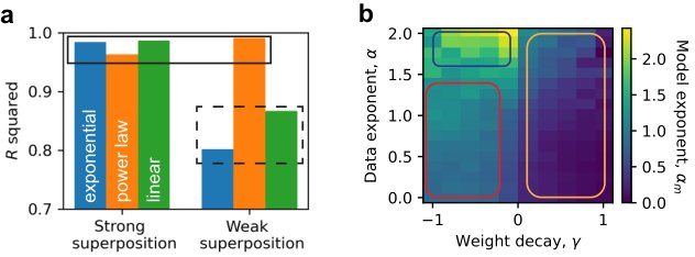
Figure 9: Row norm distributions for large toy models. There are 6 rows of panels. Rows 1 and 2 correspond to the power-law feature frequency. Rows 3 and 4 correspond to the exponential feature frequency. Rows 5 and 6 correspond to the exponential feature frequency. In the two rows that correspond to the same feature frequency, the upper row is at strong superposition and the lower one is at weak superposition. The 8 columns from left to right correspond to different model dimensions from small to large.
图 9:大型玩具模型的行范数分布。共 6 行面板。第 1、2 行对应幂律特征频率;第 3、4 行对应指数特征频率;第 5、6 行对应线性特征频率。同频率的两行中,上行为强叠加、下行为弱叠加。从左到右 8 列对应从小到大的不同模型维 。
We also output the weight matrix for these large toy models (Figure 9). They follow the same pattern that in the weak superposition regime, row norms are bimodal and are either close to or , making a good separation point for measuring how many features are represented. And in the strong superposition regime, the row norms are distributed near , and is a good separation point for the two peaks, i.e., the peak greater than 1 refers to strongly represented features which are more important, and the peak smaller than 1 corresponds to the weakly represented.
我们也输出这些大型玩具模型的权矩阵 (图 9)。模式一致:弱叠加区行范数双峰,接近 或 ,使 成为度量已表示特征数的良好分界;强叠加区行范数分布在 附近, 是两峰的良好分界——大于 1 的峰对应更重要的强表示特征,小于 1 的峰对应弱表示。
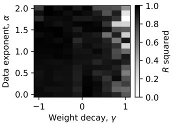
Figure 10: Large toy models agree with theoretical expectations. We use blue, yellow, and green for exponential, power-law, and linear feature frequencies, respectively. Dots correspond to the weak superposition regime, and squares to the strong superposition regime. (a) The fraction of represented features is for strong superposition, and is close to (black dashed line). (b) The expected number of activated but unlearned features well describes the loss at weak superposition. The dashed line is where the actual loss is the same as the predicted one. (c) In the strong superposition regime, the number of strongly represented features is much larger than but bounded by some value around . The slowly growing dashed line is , and the fast growing dashed line is . (d) The mean squared overlap of strongly represented features is close to , which is close to , given that the number of strongly represented features is much larger than .
图 10:大型玩具模型与理论期望吻合。蓝、黄、绿分别对应指数、幂律与线性特征频率。圆点为弱叠加,方块为强叠加。(a)已表示特征比例:强叠加为 ,弱叠加接近 (黑虚线)。(b)被激活但未学习特征的期望数很好描述弱叠加损失;虚线为实际损失等于预测处。(c)强叠加下强表示特征数远大于 ,但被约 的某值上界;缓慢上升虚线为 ,快速上升虚线为 。(d)强表示特征的均方重叠接近 ,因强表示数远大于 ,故接近 。
We can analyze the large toy model in the same way as what has been done in Figure 5 and 6. The fraction of represented features is calculated, which is 1 in the strong superposition regime, while it is close to in the weak superposition regime (Figure 10a).
可用与图 5、6 相同方式分析大型玩具模型。计算已表示特征比例 :强叠加为 1,弱叠加接近 (图 10a)。
With the measured , we can estimate the loss due to unlearned features, . This loss by unlearned features agrees well with the actual loss in the weak superposition regime (Figure 10b).
用测得的 ,可估计未学习特征带来的损失 。该损失在弱叠加区与实际损失吻合良好(图 10b)。
In the strong superposition regime, the fraction of strongly represented features is calculated, agreeing with the expectation that the number of strongly represented features is much larger than but bounded by some value around (Figure 10c).
强叠加区计算强表示特征比例,与「强表示数远大于 但被约 上界」的期望一致(图 10c)。
At the end, we see that the mean square overlap of the strongly represented is close to the characterized value (Figure 10d), which scales as since the number of the strongly represented is much larger than .
最后,强表示的均方重叠接近刻画值 (图 10d);因强表示数远大于 ,故按 缩放。
D.2 Figure 2
Figure 2 introduced the toy model and the concept of superposition without real data. The matrix we used to show superposition in Figure 2c is obtained by optimizing the square of off-diagonal terms of the normalized , i.e., each row is normalized to have norm 1 first.
图 2 在无真实数据下引入玩具模型与叠加概念。图 2c 用于展示叠加的 矩阵,通过对归一化 的非对角项平方做优化得到——即先把每行归一化为范数 1。
D.3 Figure 3
In Figure 3, we reported results from the trained small toy models with data dimension , whose details are in Appendix B.2.
图 3 报告的是数据维 的已训小型玩具模型结果,细节见附录 B.2。
We showed results at data exponent in Figure 3a. The inner panels are obtained at . We showed that the more frequent features tend to have larger norms or to be better represented. And the norm distribution is very bimodal. We here show that it is true that the norm is around or for various and model sizes and degrees of superposition (Figures 11 and 12). The fraction of represented, , can be calculated directly.
图 3a 展示数据指数 的结果;内嵌面板取自 。我们显示更频繁特征倾向于有更大范数或被更好表示,且范数分布高度双峰。这里进一步表明:对各种 、模型规模 与叠加程度,范数都约在 或 (图 11、12)。已表示比例 可直接计算。
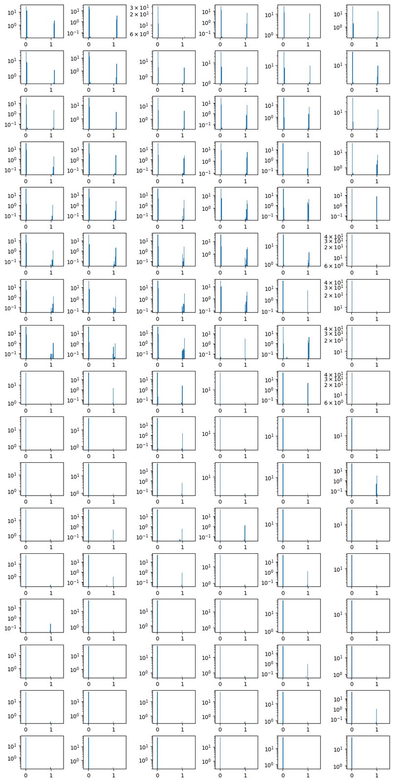
Figure 11: Row norm distribution at weak superposition () shows that the rows either are close to zero or have norm close to 1, making a good separation. The 17 rows of panels from top to down correspond to 17 from 0 to 2. And the 6 columns from left to right correspond to 6 from to .
图 11:弱叠加()下行范数分布显示:行要么接近零,要么范数接近 1,使 成为良好分界。自上而下 17 行对应 从 0 到 2;从左到右 6 列对应 从 到 。
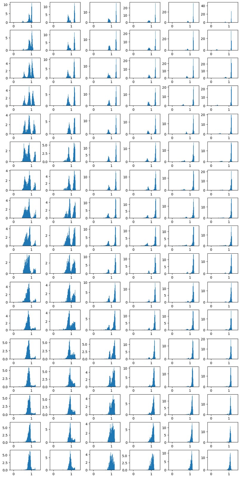
Figure 12: Row norm distribution at strong superposition () shows that the rows have norm close to 1. And density at is very low, making a good separation point for two groups of row norms. The 17 rows of panels from top to down correspond to 17 from 0 to 2. And the 6 columns from left to right correspond to 6 from to .
图 12:强叠加()下行范数分布显示行范数接近 1;在 处密度很低,使 成为两组行范数的良好分界。自上而下 17 行对应 从 0 到 2;从左到右 6 列对应 从 到 。
We next showed the as a function of and at . Here, we provide the same plot but at different (Figure 13). The pattern is robust, suggesting weight decay is a good tool to change the degree of superposition.
接着在 展示 作为 与 的函数。这里给出不同 下的相同图(图 13)。模式稳健,表明权重衰减是改变叠加程度的良好工具。

Figure 13: Fraction of represented features as a function of (x-axis) and (y-axis). The 6 columns from left to right correspond to 6 from to . The colorbar is the same as the main text (Figure 3b) where purple means .
图 13:已表示特征比例作为 (横轴)与 (纵轴)的函数。从左到右 6 列对应 从 到 。色条与正文(图 3b)相同,紫色表示 。
D.4 Figure 4
Figure 4a reports the values from the fitting introduced in Appendix D.1, where the raw data comes from training large toy models (Appendix B.1). When we are fitting the loss in log-log as a line, we choose the linear part to fit. If the loss versus model dimension curve is obviously not a line, we fit the whole curve as a line and output the value as a measure of how non-linear it is. Specifically, we fit the last five points for the power-law decay feature case in the weak superposition regime (yellow data in Figure 1b). Other cases in the weak superposition regime are fitted to a line with all data. In the strong superposition regime, when feature frequency decreases as a power law or as a linear function, we fit the data as a line starting from the third point (yellow and green in Figure 1d).
图 4a 报告附录 D.1 所述拟合的 ,原始数据来自训练大型玩具模型(附录 B.1)。在双对数上把损失拟成直线时选线性段;若曲线明显非直线,则整条按直线拟合并以 度量非线性。具体地,弱叠加区幂律衰减特征情形(图 1b 黄)拟合最后五点;弱叠加其他情形用全部数据。强叠加区特征频率按幂律或线性下降时,从第三点起拟合(图 1d 黄、绿)。
And from the raw data of small toy models (Appendix B.2), we can fit the model exponent directly and plot it as a function of and as in Figure 4b.
由小型玩具模型原始数据(附录 B.2),可直接拟合模型指数 ,并像图 4b 那样画成 与 的函数。
The fitting in Figure 4b does not care whether the loss versus model dimension curve is a power law or not. We provide the squared values for the fitting here (Figure 14). The closer squared values are to , the better the data can be thought to be a power law (a line in log-log plot). In the strong superposition regime, the squared values suggest the data are close to be power-law. While in the weak superposition regime, data may not be power-law, especially when is too large. When is smaller than , it is not a power law in theory. The squared values are not too small since the loss decay is very slow, and a line in log-log plot is still a good approximation. When and , the number of represented features can be smaller than or even non-increasing. Too large weight decay still makes the configuration of the representation be in no superposition. However, it destroys some feature representations that can exist, making the configuration far from the ideal case where features are represented. So, we may not see power laws when weight decay is too strong.
图 4b 的拟合不关心损失相对模型维是否幂律。这里给出拟合的 方(图 14)。 方越接近 ,数据越可视为幂律(双对数上的直线)。强叠加区 方表明数据接近幂律;弱叠加区则未必,尤其 过大时。当 小于 ,理论上本非幂律; 方不太小是因为损失衰减很慢,双对数直线仍是不错逼近。当 且 时,已表示特征数可小于 甚至不增。过大权重衰减仍使表征配置处于无叠加,但会毁掉本可存在的部分特征表示,使配置远离「 个特征被完美表示」的理想情形。因此权重衰减过强时可能看不到幂律。
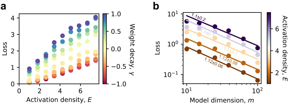
Figure 14: R squared values for fitting loss as a power law with model dimension. Data are from the small toy models with data dimension .
图 14:把损失拟成随模型维幂律时的 R 方。数据来自数据维 的小型玩具模型。
D.5 Figure 5
In Figure 5a, we plot the raw losses from small toy model experiments (Appendix B.2). The “loss by unlearned" is approximated by the integral, which is
图 5a 画出小型玩具模型实验(附录 B.2)的原始损失。「未学习带来的损失」用积分逼近,为
$$L=\left{\begin{aligned} &\frac{\phi_{1/2}^{1-\alpha}-1}{1-n^{1-\alpha}}n^{1-\alpha},\alpha\neq 1,\\alpha=1.\end{aligned}\right.$$
&-\frac{\ln\phi_{1/2}}{\ln n},
To quantify how much the learned weight matrix deviates from the ideal no superposition structure, we construct a reference matrix and compute a norm difference. Specifically, we first create an -by- zero matrix called base, and then insert an identity matrix of size in its top-left corner. This padded identity matrix serves as a reference for the perfect recovery of the first features. We then compute the matrix product from the learned weights and compare it to this reference using the matrix 2-norm. The resulting value reflects the ambiguity or interference in the learned representations. We store this norm in the ambiguity tensor at the location indexed by the current task and model width. Given a weight decay and data exponent, we have 6 ambiguity values since we have 6 values. We calculate maximum ambiguity among these 6 models, and choose the 9 cases with the smallest maximum ambiguity to plot in Figure 5b. One can see that when weight decay is near , the models are closest to the ideal no superposition case where the first features are represented perfectly. Smaller weight decay may not be sufficient to eliminate superposition, and larger weight decay can suppress features that, in principle, can be represented perfectly.
为量化已学权矩阵相对理想无叠加结构的偏离,我们构造参考矩阵并算范数差。具体地,先建 零矩阵 base,再在左上角插入大小为 的单位阵;该填充单位阵作为前 个特征完美恢复的参考。然后从已学权重算 ,用矩阵 2-范数与参考比较;所得值反映已学表征中的含糊或干扰。把该范数存入以当前任务与模型宽度索引的 ambiguity 张量。给定权重衰减与数据指数,有 6 个 故有 6 个 ambiguity 值;取这 6 个中的最大 ambiguity,再选最大 ambiguity 最小的 9 个情形画在图 5b。可见权重衰减接近 时,模型最接近「前 个特征被完美表示」的理想无叠加。更小权重衰减可能不足以消除叠加,更大则可能压制原则上可完美表示的特征。
D.6 Figure 6
Figure 6 studies the results from small toy models (Appendix B.2) focusing on the strong superposition regime. For the strongly represented fraction, , we can directly compute based on the definition and the obtained weight matrices (Figure 6, a, b, and c). Here, we provide more data to show that is a natural separation point in norm to determine which are strongly represented and which are weakly represented (Figure 12).
图 6 研究小型玩具模型(附录 B.2)在强叠加区的结果。对强表示比例 ,可按定义与所得权矩阵直接计算(图 6a、b、c)。这里提供更多数据,表明用范数 作为分界以区分强/弱表示是自然的(图 12)。
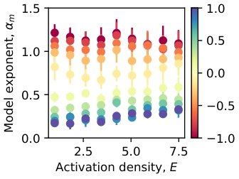
Figure 15: The overlap variance of the strongly represented is smaller than that of random vectors. We calculate the absolute overlaps of the strongly represented and can calculate the variance. We plot variance versus model dimension for different (denoted by color) and weight decays (all the negative weight decays). The dashed line is obtained by sampling Gaussian random vectors, normalizing them to have norm 1, calculating the absolute overlaps, and calculating the variance of the overlaps.
图 15:强表示的重叠方差小于随机向量。我们计算强表示的绝对重叠并可算方差;对不同 (颜色)与权重衰减(所有负权重衰减)画出方差相对模型维。虚线由采样 个高斯随机向量、归一化为范数 1、算绝对重叠再算重叠方差得到。
Once select the rows with norm greater than 1, we can calculate their mean square overlap based on normalized rows (Figure 6d). We argue that after training, the vectors will be more similar to ETFs than to random initialization. This is studied via the variance of overlaps. ETFs, in theory, have zero variance. We find that the majority of the overlap variances are much smaller than the random initialization, especially when features have similar frequencies, which agrees with the expectation (Figure 15). The cases where the actual variance is greater than that of the random vectors have large , roughly correspond to the cases where deviates from — ETF-like configuration no longer dominates. This is intuitive that when is too large, the heterogeneity of overlaps will become large — it is better to let more frequent features occupy larger angle space. We argue that the large variance at large does not mean the configuration tends to be random, but tends to be something more closely related to the frequency distribution of the features.
选出范数大于 1 的行后,可基于归一化行 计算其均方重叠(图 6d)。我们论证训后向量比随机初始化更接近 ETF;这通过重叠方差研究。理论上 ETF 方差为零。我们发现多数重叠方差远小于随机初始化,尤其在特征频率相近时,与期望一致(图 15)。实际方差大于随机向量的情形对应大 ,大致对应 偏离 ——ETF 类配置不再主导。直观上 过大时重叠异质性变大——更应让更频繁特征占据更大角度空间。我们主张大 下的大方差不意味着配置趋向随机,而趋向与特征频率分布更密切相关的某种结构。
As a related side note, our explanations based on the strongly and weakly represented features capture the basic trend that when is getting large, the more important features will have larger angle space and the loss decay will be more related to the data exponent. However, this theory is oversimplified, where the strongly represented all have small overlaps and the weakly represented all have large overlaps. The real situation may be more like the angle occupied by one feature decreases continuously as the frequency decreases. As suggested by Figure 15, overlap variance within the strongly represented is greater when is larger. To be more precise about the overlap distribution as well as the exponent when is large, we cannot use simple theoretical expectations like ETFs but have to solve the toy model.
相关附带说明:基于强/弱表示特征的解释抓住了基本趋势——随 变大,更重要特征占更大角度空间,损失衰减更与数据指数相关。但该理论过度简化:假定强表示皆小重叠、弱表示皆大重叠。真实情况更可能是:单特征所占角度随频率下降而连续减小。如图 15 所示, 更大时强表示内部的重叠方差更大。要对大 时的重叠分布与指数 更精确,不能再用 ETF 等简单理论期望,而须求解玩具模型。
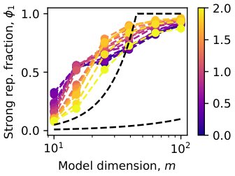
Figure 16: The weakly represented features can have large overlaps as expected, where we plotted all the data when , and the dashed line is . The colorbar corresponds to in the same way as the main text.
图 16:弱表示特征可如预期有大重叠;图中画出 的全部数据,虚线为 。色条对应 ,方式与正文相同。
We also provide evidence that overlaps of the weakly represented (Figure 16). We see that all the mean square overlaps are larger than instead of being on the line . And some values are around and not decreasing much with increasing model size , supporting our picture that the less frequent features are squeezed into a region and have large overlaps.
我们也给出弱表示重叠的证据(图 16)。可见所有均方重叠都大于 ,而非落在 线上;部分值约在 且随模型规模 增大下降不多,支持「较少频特征被挤入一区域并有大重叠」的图景。
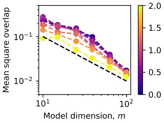
Figure 17: Small toy models with from to (such that ) in the strong superposition regime yield similar around 1 when is small and a slightly smaller (smaller than ) when is large. We copied Figure 6e and made the points transparent for comparison. The non-transparent points are from small toy models with from to . is the horizontal line, is the fast increasing dashed line, and is the slowly increasing dashed line. Error bars are standard errors.
图 17:强叠加区 从 到 (使 )的小型玩具模型:当 小时给出类似的 约 1;当 大时 略小(小于 )。我们复制图 6e 并将点半透明以便比较;不透明点来自 从 到 的小型玩具模型。 为水平线, 为快速上升虚线, 为缓慢上升虚线。误差棒为标准误。
After fitting of the trained small toy models (Appendix B.2), we plotted the corresponding to the second to the fourth smallest weight decays in Figure 6e. We also copied from Figure 5b and plotted the ideal weak superposition case in Figure 6e. One question we had is that if is always greater than , in our analysis, all vectors can be strongly represented, what should be? We trained the small toy models again as in Appendix B.2 but with from to . We found that in the strong superposition regime, the is still around when is smaller than , and still increases a little while smaller than when is larger than (Figure 17). When is always true, the vectors can be put into a configuration where all overlaps are small and scale as , such that should be closer to . However, as mentioned before, our picture that the strongly represented have nearly uniform absolute overlaps is oversimplified. In the real situation, more frequent features have smaller or even faster decaying overlaps. Therefore, when is too large, a weighted sum of squared overlaps, weighting the more frequent features more, can decrease faster than the average decaying speed . Again, we need to solve the toy model faithfully to uncover the rigorous relation between and and argue the robustness of from theory.
拟合已训小型玩具模型(附录 B.2)的 后,我们在图 6e 画出对应第二至第四小权重衰减的 ;并从图 5b 复制理想弱叠加情形画入图 6e。一个问题是:若 始终大于 ,按我们的分析所有向量都可强表示, 应为何?我们按附录 B.2 再训小型玩具模型但取 从 到 。发现强叠加区: 小于 时 仍约 ; 大于 时 仍略增但小于 (图 17)。当 始终成立时,向量可放入所有重叠都小并按 缩放的配置,故 应更接近 。但如前所述,「强表示具有近均匀绝对重叠」的图景过度简化;真实情形中更频繁特征有更小甚至衰减更快的重叠。因此当 过大时,对更频繁特征加权更重的重叠平方加权和,可衰减得比平均速度 更快。同样,须忠实求解玩具模型,才能揭示 与 的严格关系,并从理论上论证 的稳健性。
D.7 Figure 7
Once obtaining the small toy models scanning activation density and keeping , we can plot the loss as a function of activation density in Figure 7. The linear fitting is also straightforward. We chose one to show in the main text. Here, we present the whole picture that, with any weight decay tested, the model exponent is robust to the change of activation density (Figure 18).
得到扫描激活密度并保持 的小型玩具模型后,可在图 7 画出损失作为激活密度 的函数;线性拟合也很直接。正文选一个 展示。这里给出全貌:在任何测试的权重衰减下,模型指数对激活密度变化都稳健(图 18)。
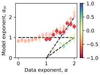
Figure 18: Model exponent is robust to activation density at different levels of superposition. The colorbar encodes weight decay as in the main text. Error bars are standard errors.
图 18:不同叠加水平下模型指数对激活密度稳健。色条按正文编码权重衰减。误差棒为标准误。
D.8 Figure 8
After obtaining the overlaps as described in Appendix C.1, we directly plot the raw data in Figure 8a. The data are quite noisy, and we did not fit the data with a line.
按附录 C.1 得到重叠后,我们直接在图 8a 画出原始数据。数据相当嘈杂,未做直线拟合。
We argued that the LLMs are in the strong superposition regime since all tokens are represented. Figure 19 shows a typical row norm distribution of LLM (opt, 125M parameters [38]). We showed the mean, minimum, and maximum row norms of all the LLMs studied in Figure 20. From the non-zero minimum norms and the fact , we confirm LLMs are in strong superposition. As mentioned in the analysis in Appendix A.2, we argue that the row norm of LLMs should not depend on but controlled more by the intrinsic data property of language, which is also verified to be valid (Figure 20).
我们主张 LLM 处于强叠加区,因所有 token 都被表示。图 19 给出典型 LLM(OPT,1.25 亿参数 [38])的行范数分布。图 20 展示所研究全部 LLM 的行范数均值、最小与最大。由非零最小范数以及 ,我们确认 LLM 处于强叠加。如附录 A.2 分析所述,我们主张 LLM 行范数不应依赖 ,而更多由语言的内在数据性质控制——亦已验证成立(图 20)。
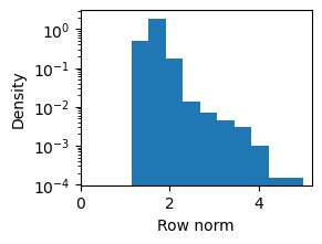
Figure 19: Row norm distribution of the language model head of OPT-125M.
图 19:OPT-125M 语言模型头的行范数分布。
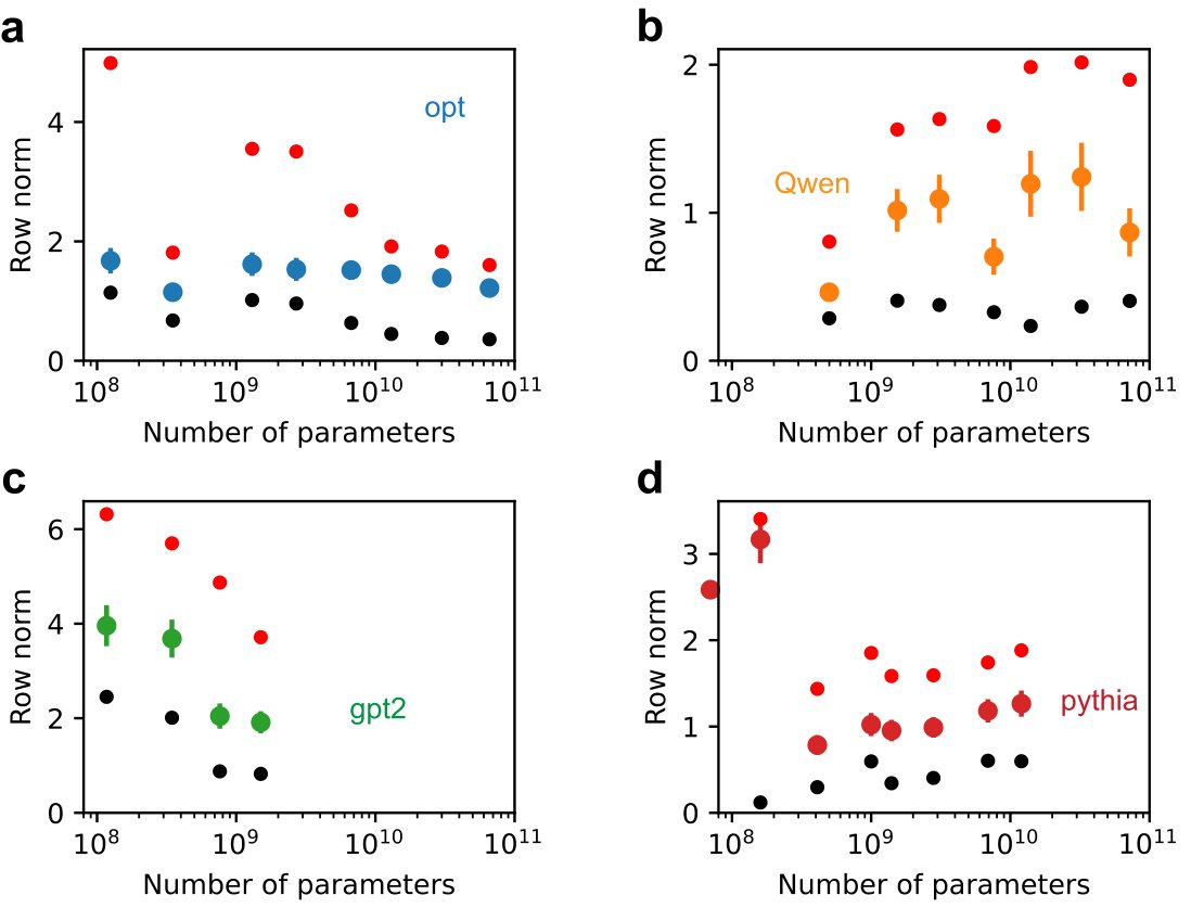
Figure 20: LLMs are in strong superposition based on the non-zero norms of the representation vectors. (a) OPT models. (b) Qwen2.5 models. (c) GPT-2 models. (d) Pythia models. The dots with error bars are mean values, and the error bar is the standard deviation. Red small points are the maximum values, and dark small points are the minimum values. The mean norm value as a characteristic row norm does not depend on model size much as expected (Appendix A.2).
图 20:基于表征向量非零范数,LLM 处于强叠加。(a)OPT 模型。(b)Qwen2.5 模型。(c)GPT-2 模型。(d)Pythia 模型。带误差棒的点为均值,误差棒为标准差;红小点为最大值,黑小点为最小值。作为特征性行范数的均值范数如预期不太依赖模型规模(附录 A.2)。
We obtain the evaluation loss of each model on each dataset as described in Appendix C.2. We fit our loss values by the formula,
按附录 C.2 得到每个模型在每个数据集上的评估损失。我们用下式拟合损失值:
where is universal and is a constant depending on the dataset and model class. There are in total different since we have different model classes and 4 datasets. In our fitting model, there are in total parameters. We use Adam to minimize the mean square error between the predicted loss by the above function and the real loss. All losses obtained are used in optimization. The code is in nonlinearfit-3.ipynb.
其中 具有普适性, 为依赖数据集与模型类的常数。因有 4 个模型类与 4 个数据集,共 个不同的 。拟合模型共 个参数。我们用 Adam 最小化上式预测损失与真实损失之间的均方误差;所有得到的损失都参与优化。代码见 nonlinearfit-3.ipynb。
We provide the raw data, losses, as a function of (Figure 21). The losses looks like a line with in one model class and with the same dataset. And the slope of the line seems to be universal. These two points support us in proposing the formula above, where is universal. The intersections are different depending on the dataset and model class, corresponding to different .
我们给出原始数据:损失作为 的函数(图 21)。在同一模型类与同一数据集上,损失看起来像随 的直线,且斜率似乎普适。这两点支持我们提出上式——其中 普适。截距因数据集与模型类而异,对应不同的 。
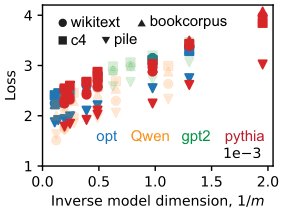
Figure 21: Raw evaluation losses as a function of inverse model dimension.
图 21:原始评估损失作为模型维倒数的函数。
We obtained the token frequencies as described in Appendix C.3. Given the raw data, we sort the token frequency and obtain the frequency-rank plot. We sample 1000 (this number does not matter once it is large, 10000 gives the same result) points uniformly in the (Rank), and fit the frequency-rank as a power law, or a line in log-log plot. Results show that the data exponent fitted is close to regardless of the dataset or the tokenizer (Figure 22).
按附录 C.3 得到 token 频率。给定原始数据,对 token 频率排序得到频率–秩图。在 (秩)上均匀采样 1000 点(该数只要大就无关紧要,10000 给出相同结果),把频率–秩拟成幂律,或双对数上的直线。结果显示:不论数据集或分词器,拟合的数据指数 都接近 (图 22)。
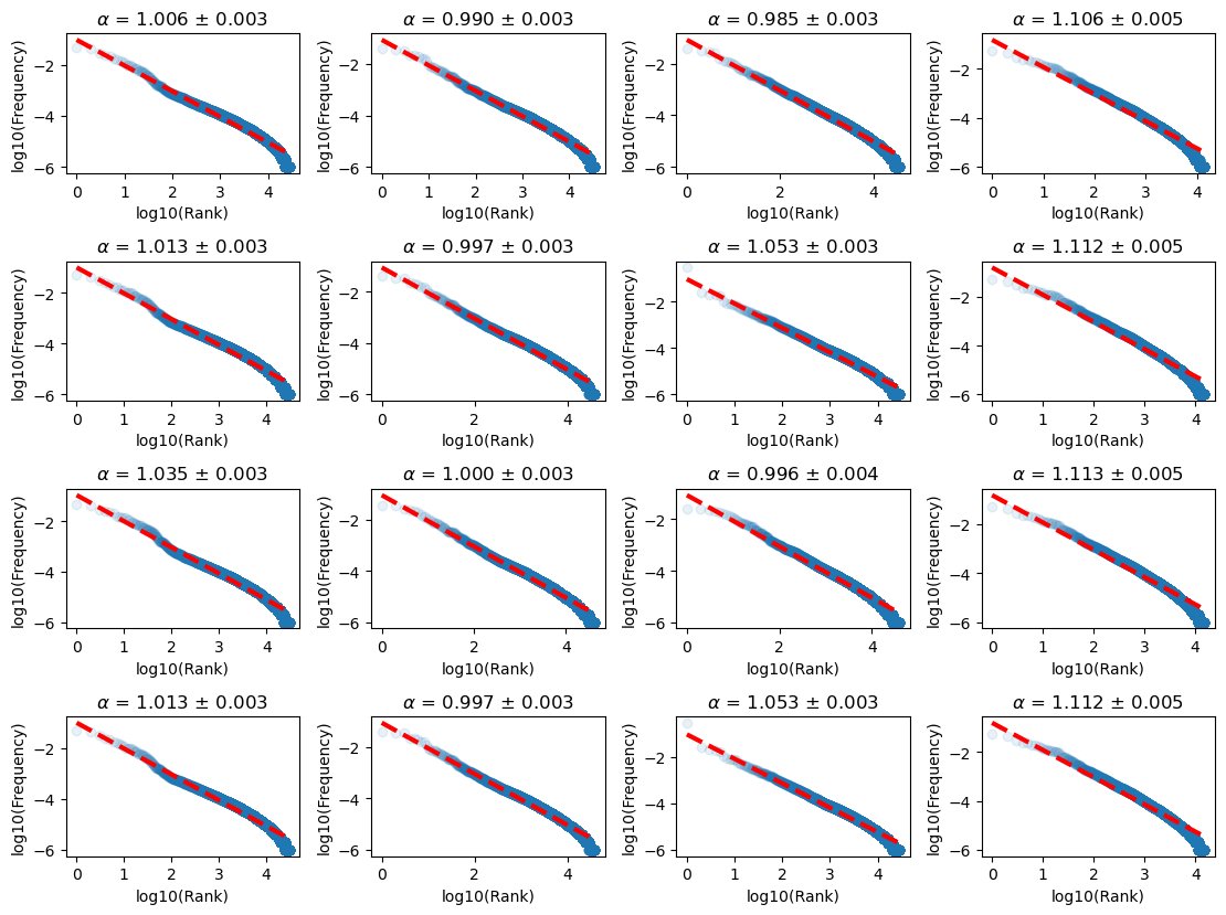
Figure 22: Taking tokens as atomic features, their frequencies indeed follow a power law, and the measured data exponent is close to 1. The four rows from top to bottom correspond to four tokenziers, Pythia, OPT, Qwen2.5, and GPT-2, respectively. And the four columns from left to right correspond to four datasets analyzed, wikitext, C4, the Pile, and Bookcorpus, respectively.
图 22:把 token 当作原子特征,其频率确实服从幂律,测得数据指数 接近 1。自上而下四行对应四种分词器:Pythia、OPT、Qwen2.5、GPT-2;从左到右四列对应四个分析数据集:wikitext、C4、the Pile、Bookcorpus。
We study the relationship between model dimension and model size (number of parameters). For the four open-sourced models we analyzed [38, 39, 40, 41], we can see that , especially when is large. If we fit the - relation by a power law while assuming a universal exponent but different coefficients depending on the model class, we obtain an exponent of (Figure 23a). For the Chinchilla model reported in [3], we find is also close to a power law with the model dimension, and the fitted exponent is (Figure 23b).
我们研究模型维 与模型规模 (参数量)的关系。对我们分析的四个开源模型 [38, 39, 40, 41],可见 ,尤其当 大时。若假定普适指数、系数因模型类而异,用幂律拟合 – 关系,得指数 (图 23a)。对 [3] 报告的 Chinchilla 模型, 也接近随模型维的幂律,拟合指数为 (图 23b)。
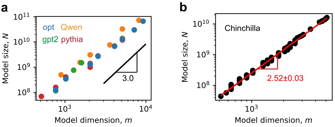
Figure 23: The model size is approximately a power law with model dimension. (a) The four model classes we analyzed [38, 39, 40, 41]. (b) The Chinchilla models [3].
图 23:模型规模近似为模型维的幂律。(a)我们分析的四个模型类 [38, 39, 40, 41]。(b)Chinchilla 模型 [3]。