Analyzing and Improving the Image Quality of StyleGAN
Analyzing and Improving the Image Quality of StyleGAN
分析并改进 StyleGAN 的图像质量
Tero Karras Affiliation: NVIDIA Samuli Laine Affiliation: NVIDIA Miika Aittala Affiliation: NVIDIA Janne Hellsten Affiliation: NVIDIA Jaakko Lehtinen Affiliation: NVIDIA and Aalto University Timo Aila Affiliation: NVIDIA
Abstract
摘要
The style-based GAN architecture (StyleGAN) yields state-of-the-art results in data-driven unconditional generative image modeling. We expose and analyze several of its characteristic artifacts, and propose changes in both model architecture and training methods to address them. In particular, we redesign the generator normalization, revisit progressive growing, and regularize the generator to encourage good conditioning in the mapping from latent codes to images. In addition to improving image quality, this path length regularizer yields the additional benefit that the generator becomes significantly easier to invert. This makes it possible to reliably attribute a generated image to a particular network. We furthermore visualize how well the generator utilizes its output resolution, and identify a capacity problem, motivating us to train larger models for additional quality improvements. Overall, our improved model redefines the state of the art in unconditional image modeling, both in terms of existing distribution quality metrics as well as perceived image quality.
基于风格的 GAN 架构(StyleGAN)在数据驱动的无条件图像生成上达到了当时最优水平。我们揭示并分析了其若干典型伪影,并在模型结构与训练方法上提出改动加以消除。具体而言,我们重新设计了生成器的归一化,重新审视渐进式增长,并对生成器施加正则,使其从潜码到图像的映射具有更好的条件数。路径长度正则除了提升画质,还显著降低了生成器求逆的难度,从而可以把生成图像可靠地归因到某一特定网络。我们还可视化了生成器对输出分辨率的利用程度,发现容量不足,据此训练更大模型以进一步提质。总体而言,改进后的模型在无条件图像建模上重新定义了当时最优水平,无论是现有分布质量指标还是主观画质。
1 Introduction
1 引言
The resolution and quality of images produced by generative methods, especially generative adversarial networks (GAN) [16], are improving rapidly [23, 31, 5]. The current state-of-the-art method for high-resolution image synthesis is StyleGAN [24], which has been shown to work reliably on a variety of datasets. Our work focuses on fixing its characteristic artifacts and improving the result quality further.
生成方法——尤其是生成对抗网络(GAN)[16]——产出图像的分辨率与质量正在快速提升[23, 31, 5]。当前高分辨率图像合成的最优方法之一是 StyleGAN [24],它在多种数据集上表现稳定。本文聚焦于修复其特有伪影,并进一步提升结果质量。
The distinguishing feature of StyleGAN [24] is its unconventional generator architecture. Instead of feeding the input latent code only to the beginning of a the network, the mapping network first transforms it to an intermediate latent code . Affine transforms then produce styles that control the layers of the synthesis network via adaptive instance normalization (AdaIN) [21, 9, 13, 8]. Additionally, stochastic variation is facilitated by providing additional random noise maps to the synthesis network. It has been demonstrated [24, 38] that this design allows the intermediate latent space to be much less entangled than the input latent space . In this paper, we focus all analysis solely on , as it is the relevant latent space from the synthesis network’s point of view.
StyleGAN [24] 的标志性特点是非常规的生成器结构。输入潜码 并不只接到网络起点,而是先由映射网络 变换为中间潜码 ;再经仿射变换得到风格,通过自适应实例归一化(AdaIN)[21, 9, 13, 8] 控制合成网络 的各层。此外,还向合成网络注入额外的随机噪声图以提供随机变化。已有工作[24, 38]表明,该设计使中间潜空间 的纠缠远弱于输入潜空间 。本文分析全部聚焦于 ,因为它才是从合成网络视角相关的潜空间。

Figure 1: Instance normalization causes water droplet -like artifacts in StyleGAN images. These are not always obvious in the generated images, but if we look at the activations inside the generator network, the problem is always there, in all feature maps starting from the 64x64 resolution. It is a systemic problem that plagues all StyleGAN images.
图 1:实例归一化在 StyleGAN 图像中造成水滴状伪影。它们在最终图像上未必显眼,但查看生成器内部激活时,从 分辨率起,所有特征图上都始终存在。这是困扰所有 StyleGAN 图像的系统性问题。
Many observers have noticed characteristic artifacts in images generated by StyleGAN [3]. We identify two causes for these artifacts, and describe changes in architecture and training methods that eliminate them. First, we investigate the origin of common blob-like artifacts, and find that the generator creates them to circumvent a design flaw in its architecture. In Section 2, we redesign the normalization used in the generator, which removes the artifacts. Second, we analyze artifacts related to progressive growing [23] that has been highly successful in stabilizing high-resolution GAN training. We propose an alternative design that achieves the same goal — training starts by focusing on low-resolution images and then progressively shifts focus to higher and higher resolutions — without changing the network topology during training. This new design also allows us to reason about the effective resolution of the generated images, which turns out to be lower than expected, motivating a capacity increase (Section 4).
许多观察者已注意到 StyleGAN 生成图像中的特征性伪影[3]。我们找出两类原因,并给出可消除它们的结构与训练改动。首先,我们追查常见的团块状伪影来源,发现生成器是在绕过结构上的设计缺陷而主动制造它们。第 2 节我们重新设计生成器中的归一化,伪影随之消失。其次,我们分析与渐进式增长[23]相关的伪影——该方法虽极有助于稳住高分辨率 GAN 训练。我们提出一种替代设计,达到同一目标——训练先聚焦低分辨率图像,再逐步把注意力移向更高分辨率——且训练过程中不必改动网络拓扑。新设计也让我们能讨论生成图像的有效分辨率;该分辨率低于预期,从而促使我们增加容量(第 4 节)。
Quantitative analysis of the quality of images produced using generative methods continues to be a challenging topic. Fréchet inception distance (FID) [20] measures differences in the density of two distributions in the high-dimensional feature space of an InceptionV3 classifier [39]. Precision and Recall (P&R) [36, 27] provide additional visibility by explicitly quantifying the percentage of generated images that are similar to training data and the percentage of training data that can be generated, respectively. We use these metrics to quantify the improvements.
对生成图像质量做定量分析仍是难题。Fréchet inception distance(FID)[20] 在 InceptionV3 分类器[39]的高维特征空间中度量两个分布密度的差异。Precision and Recall(P&R)[36, 27] 则分别量化「有多少生成图像与训练数据相似」以及「有多少训练数据可被生成」,提供额外可见性。我们用这些指标量化改进。
Both FID and P&R are based on classifier networks that have recently been shown to focus on textures rather than shapes [12], and consequently, the metrics do not accurately capture all aspects of image quality. We observe that the perceptual path length (PPL) metric [24], originally introduced as a method for estimating the quality of latent space interpolations, correlates with consistency and stability of shapes. Based on this, we regularize the synthesis network to favor smooth mappings (Section 3) and achieve a clear improvement in quality. To counter its computational expense, we also propose executing all regularizations less frequently, observing that this can be done without compromising effectiveness.
FID 与 P&R 都依赖分类器网络,而近期研究表明这类网络更关注纹理而非形状[12],因此指标并不能准确刻画画质的所有方面。我们观察到,最初用于估计潜空间插值质量的感知路径长度(PPL)指标[24]与形状一致性、稳定性相关。据此,我们对合成网络施加偏好平滑映射的正则(第 3 节),画质明显提升。为抵消其计算开销,我们还提出降低所有正则的执行频率,并观察到这样做并不损害效果。
Finally, we find that projection of images to the latent space works significantly better with the new, path-length regularized StyleGAN2 generator than with the original StyleGAN. This makes it easier to attribute a generated image to its source (Section 5).
最后我们发现,把图像投影到潜空间 时,带路径长度正则的新 StyleGAN2 生成器显著优于原始 StyleGAN,从而更容易把生成图像归因到其来源(第 5 节)。
Our implementation and trained models are available at https://github.com/NVlabs/stylegan2
实现与训练好的模型见 https://github.com/NVlabs/stylegan2
2 Removing normalization artifacts
2 消除归一化伪影
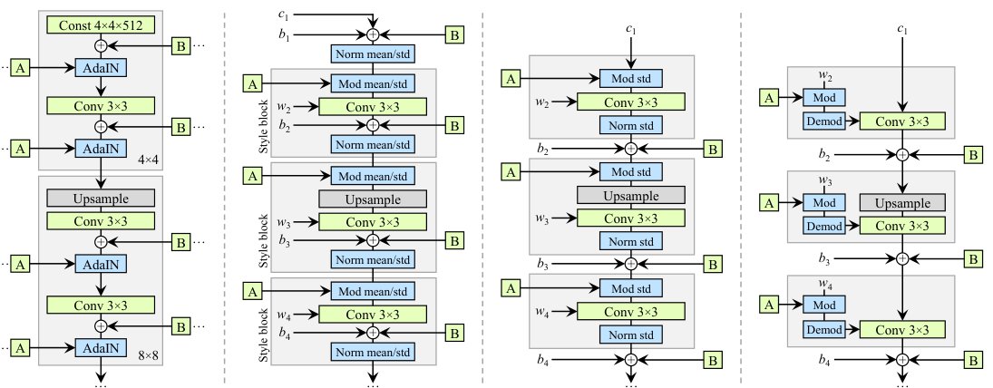
(a) StyleGAN (b) StyleGAN (detailed) (c) Revised architecture (d) Weight demodulation
Figure 2: We redesign the architecture of the StyleGAN synthesis network. (a) The original StyleGAN, where A denotes a learned affine transform from that produces a style and B is a noise broadcast operation. (b) The same diagram with full detail. Here we have broken the AdaIN to explicit normalization followed by modulation, both operating on the mean and standard deviation per feature map. We have also annotated the learned weights (), biases (, and constant input (), and redrawn the gray boxes so that one style is active per box. The activation function (leaky ReLU) is always applied right after adding the bias. (c) We make several changes to the original architecture that are justified in the main text. We remove some redundant operations at the beginning, move the addition of and B to be outside active area of a style, and adjust only the standard deviation per feature map. (d) The revised architecture enables us to replace instance normalization with a “demodulation” operation, which we apply to the weights associated with each convolution layer.
(a) StyleGAN (b) StyleGAN(细节) (c) 修订后的结构 (d) 权解调
图 2:我们重新设计 StyleGAN 合成网络的结构。(a) 原始 StyleGAN,其中 A 表示从 学到的仿射变换以产生风格,B 为噪声广播操作。(b) 同一示意图的完整细节。此处把 AdaIN 拆成显式归一化与调制,二者都对每个特征图的均值与标准差操作。我们标注了可学习权重()、偏置()与常数输入(),并重画灰色框,使每个框内只有一种风格生效。激活函数(leaky ReLU)总是在加偏置后立刻应用。(c) 我们对原结构做了正文论证的若干改动:去掉开头若干冗余操作,把 与 B 的加法移到风格作用区域之外,并且只按特征图调整标准差。(d) 修订后的结构使我们能用「解调」操作替代实例归一化,该操作作用于每个卷积层相关的权重。
We begin by observing that most images generated by StyleGAN exhibit characteristic blob-shaped artifacts that resemble water droplets. As shown in Figure 1, even when the droplet may not be obvious in the final image, it is present in the intermediate feature maps of the generator.[^1] The anomaly starts to appear around 6464 resolution, is present in all feature maps, and becomes progressively stronger at higher resolutions. The existence of such a consistent artifact is puzzling, as the discriminator should be able to detect it.
我们首先观察到,StyleGAN 生成的多数图像都带有类似水滴的特征性团块伪影。如图 1 所示,即便水滴在最终图像上不明显,它也存在于生成器的中间特征图中。[^1] 异常大约从 分辨率开始出现,存在于所有特征图,并在更高分辨率上逐渐加强。如此一致的伪影令人费解,因为判别器理应能够检出它。
We pinpoint the problem to the AdaIN operation that normalizes the mean and variance of each feature map separately, thereby potentially destroying any information found in the magnitudes of the features relative to each other. We hypothesize that the droplet artifact is a result of the generator intentionally sneaking signal strength information past instance normalization: by creating a strong, localized spike that dominates the statistics, the generator can effectively scale the signal as it likes elsewhere. Our hypothesis is supported by the finding that when the normalization step is removed from the generator, as detailed below, the droplet artifacts disappear completely.
我们把问题定位到 AdaIN:它对每个特征图分别归一化均值与方差,从而可能毁掉特征相对幅度中携带的信息。我们假设,水滴伪影是生成器有意把信号强度信息偷偷带过实例归一化的结果:制造一个支配统计量的强局域尖峰后,生成器就能在别处任意缩放信号。去掉归一化步骤后水滴完全消失(细节见下),支持这一假设。
2.1 Generator architecture revisited
2.1 重新审视生成器结构
We will first revise several details of the StyleGAN generator to better facilitate our redesigned normalization. These changes have either a neutral or small positive effect on their own in terms of quality metrics.
我们先修订 StyleGAN 生成器的若干细节,以便更好地承接重新设计的归一化。这些改动本身对质量指标呈中性或略有正向影响。
Figure 2a shows the original StyleGAN synthesis network [24], and in Figure 2b we expand the diagram to full detail by showing the weights and biases and breaking the AdaIN operation to its two constituent parts: normalization and modulation. This allows us to re-draw the conceptual gray boxes so that each box indicates the part of the network where one style is active (i.e., “style block”). Interestingly, the original StyleGAN applies bias and noise within the style block, causing their relative impact to be inversely proportional to the current style’s magnitudes. We observe that more predictable results are obtained by moving these operations outside the style block, where they operate on normalized data. Furthermore, we notice that after this change it is sufficient for the normalization and modulation to operate on the standard deviation alone (i.e., the mean is not needed). The application of bias, noise, and normalization to the constant input can also be safely removed without observable drawbacks. This variant is shown in Figure 2c, and serves as a starting point for our redesigned normalization.
图 2a 给出原始 StyleGAN 合成网络 [24];图 2b 展开完整细节,标出权重与偏置,并把 AdaIN 拆成归一化与调制两部分。据此我们重画概念上的灰色框,使每个框对应一种风格生效的网络片段(即「风格块」)。有趣的是,原 StyleGAN 在风格块内部施加偏置与噪声,使其相对影响与当前风格幅度成反比。我们观察到,把这些操作移到风格块之外、作用在已归一化的数据上,结果更可预期。进一步发现,做完这一改动后,归一化与调制只需对标准差操作(不必再管均值)。对常数输入施加偏置、噪声与归一化也可安全去掉,无明显弊端。该变体见图 2c,并作为我们重新设计归一化的起点。
2.2 Instance normalization revisited
2.2 重新审视实例归一化
One of the main strengths of StyleGAN is the ability to control the generated images via style mixing, i.e., by feeding a different latent to different layers at inference time. In practice, style modulation may amplify certain feature maps by an order of magnitude or more. For style mixing to work, we must explicitly counteract this amplification on a per-sample basis — otherwise the subsequent layers would not be able to operate on the data in a meaningful way.
StyleGAN 的一大优势是可通过风格混合控制生成图像,即在推理时向不同层喂入不同的潜码 。实践中,风格调制可能把某些特征图放大一个数量级甚至更多。为使风格混合成立,我们必须按样本显式抵消这种放大——否则后续层无法对数据做有意义的处理。
If we were willing to sacrifice scale-specific controls (see video), we could simply remove the normalization, thus removing the artifacts and also improving FID slightly [27]. We will now propose a better alternative that removes the artifacts while retaining full controllability. The main idea is to base normalization on the expected statistics of the incoming feature maps, but without explicit forcing.
若我们愿意牺牲按尺度的控制(见视频),可以干脆去掉归一化,从而消除伪影并略微改善 FID [27]。下面我们提出更好的替代方案:去掉伪影的同时保留完整可控性。核心想法是基于输入特征图的期望统计量做归一化,但不做显式强制。
Recall that a style block in Figure 2c consists of modulation, convolution, and normalization. Let us start by considering the effect of a modulation followed by a convolution. The modulation scales each input feature map of the convolution based on the incoming style, which can alternatively be implemented by scaling the convolution weights:
回顾图 2c 中的风格块:由调制、卷积与归一化组成。先考虑调制后接卷积的效果。调制按传入风格缩放卷积的每个输入特征图,这也可以等价地通过对卷积权重缩放来实现:
where and are the original and modulated weights, respectively, is the scale corresponding to the th input feature map, and and enumerate the output feature maps and spatial footprint of the convolution, respectively.
其中 与 分别为原始与调制后的权重, 是对应第 个输入特征图的尺度, 与 分别枚举输出特征图与卷积的空间支撑。
Now, the purpose of instance normalization is to essentially remove the effect of from the statistics of the convolution’s output feature maps. We observe that this goal can be achieved more directly. Let us assume that the input activations are i.i.d. random variables with unit standard deviation. After modulation and convolution, the output activations have standard deviation of
实例归一化的目的,本质上是从卷积输出特征图的统计量中去掉 的影响。我们观察到,可以更直接地达到这一目标。假设输入激活是标准差为 1 的 i.i.d. 随机变量。经调制与卷积后,输出激活的标准差为
\sigma_{j}=\sqrt{\raisebox{0.0pt}[11.38109pt][7.11317pt]{$\underset{i,k}{{}\displaystyle\sum{}}$}{w^{\prime}_{ijk}}^{2}}, \tag{2}
i.e., the outputs are scaled by the norm of the corresponding weights. The subsequent normalization aims to restore the outputs back to unit standard deviation. Based on Equation 2, this is achieved if we scale (“demodulate”) each output feature map by . Alternatively, we can again bake this into the convolution weights:
亦即,输出被对应权重的 范数所缩放。随后的归一化旨在把输出恢复为单位标准差。根据式 2,若对每个输出特征图 乘以 (「解调」),即可达到。我们同样可以把这一步烘焙进卷积权重:
w^{\prime\prime}_{ijk}=w^{\prime}_{ijk}\bigg/\sqrt{\raisebox{0.0pt}[11.38109pt][7.11317pt]{$\underset{i,k}{{}\displaystyle\sum{}}$}{w^{\prime}_{ijk}}^{2}+\epsilon}, \tag{3}
where is a small constant to avoid numerical issues.
其中 是避免数值问题的小常数。
| Configuration | FFHQ, 10241024 | LSUN Car, 512384 | |||||||
|---|---|---|---|---|---|---|---|---|---|
| FID | Path length | Precision | Recall | FID | Path length | Precision | Recall | ||
| a | Baseline StyleGAN [24] | 4.40 | 212.1 | 0.721 | 0.399 | 3.27 | 1484.5 | 0.701 | 0.435 |
| b | + Weight demodulation | 4.39 | 175.4 | 0.702 | 0.425 | 3.04 | 0862.4 | 0.685 | 0.488 |
| c | + Lazy regularization | 4.38 | 158.0 | 0.719 | 0.427 | 2.83 | 0981.6 | 0.688 | 0.493 |
| d | + Path length regularization | 4.34 | 122.5 | 0.715 | 0.418 | 3.43 | 0651.2 | 0.697 | 0.452 |
| e | + No growing, new G & D arch. | 3.31 | 124.5 | 0.705 | 0.449 | 3.19 | 0471.2 | 0.690 | 0.454 |
| f | + Large networks (StyleGAN2) | 2.84 | 145.0 | 0.689 | 0.492 | 2.32 | 0****415.5 | 0.678 | 0.514 |
| Config a with large networks | 3.98 | 199.2 | 0.716 | 0.422 | – | – | – | – |
Table 1: Main results. For each training run, we selected the training snapshot with the lowest FID. We computed each metric 10 times with different random seeds and report their average. Path length corresponds to the PPL metric, computed based on path endpoints in [24], without the central crop used by Karras et al. [24]. The FFHQ dataset contains 70k images, and the discriminator saw 25M images during training. For LSUN Car the numbers were 893k and 57M. indicates that higher is better, and that lower is better.
表 1:主要结果。每次训练我们选取 FID 最低的快照。每个指标用不同随机种子计算 10 次并报告均值。Path length 对应 PPL 指标,基于 中路径端点计算[24],且不采用 Karras 等人[24]使用的中心裁剪。FFHQ 含 70k 图像,训练中判别器见过 25M 图像;LSUN Car 对应数字为 893k 与 57M。 表示越高越好, 表示越低越好。
We have now baked the entire style block to a single convolution layer whose weights are adjusted based on using Equations 1 and 3 (Figure 2d). Compared to instance normalization, our demodulation technique is weaker because it is based on statistical assumptions about the signal instead of actual contents of the feature maps. Similar statistical analysis has been extensively used in modern network initializers [14, 19], but we are not aware of it being previously used as a replacement for data-dependent normalization. Our demodulation is also related to weight normalization [37] that performs the same calculation as a part of reparameterizing the weight tensor. Prior work has identified weight normalization as beneficial in the context of GAN training [43].
至此,整个风格块已烘焙成单一卷积层,其权重按式 1 与式 3 依据 调整(图 2d)。相对实例归一化,我们的解调更弱,因为它基于对信号的统计假设,而非特征图的实际内容。类似的统计分析在现代网络初始化中被广泛使用[14, 19],但我们尚未见到它被用作数据相关归一化的替代。我们的解调也与权归一化[37]相关,后者在对权重张量重参数化时做同样计算。已有工作指出权归一化有利于 GAN 训练[43]。
Our new design removes the characteristic artifacts (Figure 3) while retaining full controllability, as demonstrated in the accompanying video. FID remains largely unaffected (Table 1, rows a, b), but there is a notable shift from precision to recall. We argue that this is generally desirable, since recall can be traded into precision via truncation, whereas the opposite is not true [27]. In practice our design can be implemented efficiently using grouped convolutions, as detailed in Appendix B. To avoid having to account for the activation function in Equation 3, we scale our activation functions so that they retain the expected signal variance.
新设计消除了特征性伪影(图 3),同时保留完整可控性,见配套视频。FID 基本不受影响(表 1,行 a、b),但可见精度向召回的明显转移。我们认为这通常是可取的,因为召回可通过截断换成精度,反之则不行[27]。实践中可用分组卷积高效实现该设计,见附录 B。为避免在式 3 中再单独计入激活函数,我们对激活函数做缩放,使其保持期望信号方差。
3 Image quality and generator smoothness
3 图像质量与生成器平滑性

Figure 3: Replacing normalization with demodulation removes the characteristic artifacts from images and activations.
图 3:用解调替换归一化后,图像与激活中的特征性伪影消失。
While GAN metrics such as FID or Precision and Recall (P&R) successfully capture many aspects of the generator, they continue to have somewhat of a blind spot for image quality. For an example, refer to Figures 13 and 14 that contrast generators with identical FID and P&R scores but markedly different overall quality.[^2]
尽管 FID 或 Precision and Recall(P&R)等 GAN 指标能抓住生成器的许多方面,它们对画质仍有一定盲区。例如可参见图 13 与图 14:两个生成器 FID 与 P&R 相同,但整体质量明显不同。[^2]

(a) Low PPL scores (b) High PPL scores
Figure 4: Connection between perceptual path length and image quality using baseline StyleGAN (config a) with LSUN Cat. (a) Random examples with low PPL ( percentile). (b) Examples with high PPL ( percentile). There is a clear correlation between PPL scores and semantic consistency of the images.
(a) 低 PPL 分数 (b) 高 PPL 分数
图 4:在基线 StyleGAN(配置 a)与 LSUN Cat 上,感知路径长度与图像质量的关联。(a) PPL 较低( 百分位)的随机样例。(b) PPL 较高( 百分位)的样例。PPL 分数与图像语义一致性有清晰相关。
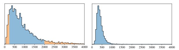
(a) StyleGAN (config a) (b) StyleGAN2 (config f)
Figure 5: (a) Distribution of PPL scores of individual images generated using baseline StyleGAN (config a) with LSUN Cat (FID = 8.53, PPL = 924). The percentile ranges corresponding to Figure 4 are highlighted in orange. (b) StyleGAN2 (config f) improves the PPL distribution considerably (showing a snapshot with the same FID = 8.53, PPL = 387).
(a) StyleGAN(配置 a) (b) StyleGAN2(配置 f)
图 5:(a) 用基线 StyleGAN(配置 a)在 LSUN Cat 上生成的单图像 PPL 分数分布(FID = 8.53,PPL = 924)。对应图 4 的百分位区间以橙色标出。(b) StyleGAN2(配置 f)显著改善了 PPL 分布(展示 FID 相同 = 8.53、PPL = 387 的快照)。
We observe a correlation between perceived image quality and perceptual path length (PPL) [24], a metric that was originally introduced for quantifying the smoothness of the mapping from a latent space to the output image by measuring average LPIPS distances [50] between generated images under small perturbations in latent space. Again consulting Figures 13 and 14, a smaller PPL (smoother generator mapping) appears to correlate with higher overall image quality, whereas other metrics are blind to the change. Figure 4 examines this correlation more closely through per-image PPL scores on LSUN Cat, computed by sampling the latent space around . Low scores are indeed indicative of high-quality images, and vice versa. Figure 5a shows the corresponding histogram and reveals the long tail of the distribution. The overall PPL for the model is simply the expected value of these per-image PPL scores. We always compute PPL for the entire image, as opposed to Karras et al. [24] who use a smaller central crop.
我们观察到主观画质与感知路径长度(PPL)[24]相关。PPL 最初用于量化从潜空间到输出图像映射的平滑性,方法是在潜空间做小扰动时测量生成图像间的平均 LPIPS 距离[50]。再看图 13 与图 14,更小的 PPL(更平滑的生成器映射)似乎对应更高的整体画质,而其他指标对这一变化视而不见。图 4 在 LSUN Cat 上用逐图像 PPL 分数更细地检验该相关,分数通过对 附近采样得到。低分确实指示高质量图像,反之亦然。图 5a 给出对应直方图,并露出分布的长尾。模型的总体 PPL 就是这些逐图像 PPL 的期望。我们始终对整幅图像计算 PPL,而不像 Karras 等人[24]那样使用较小的中心裁剪。
It is not immediately obvious why a low PPL should correlate with image quality. We hypothesize that during training, as the discriminator penalizes broken images, the most direct way for the generator to improve is to effectively stretch the region of latent space that yields good images. This would lead to the low-quality images being squeezed into small latent space regions of rapid change. While this improves the average output quality in the short term, the accumulating distortions impair the training dynamics and consequently the final image quality.
为何低 PPL 应与画质相关,并不一目了然。我们假设:训练中判别器惩罚破损图像时,生成器最直接的改进方式是有效拉伸潜空间中产出好图的区域。这会把低质量图像挤进变化剧烈的小片潜空间。短期虽提高平均输出质量,但累积畸变会损害训练动态,最终也损害画质。
Clearly, we cannot simply encourage minimal PPL since that would guide the generator toward a degenerate solution with zero recall. Instead, we will describe a new regularizer that aims for a smoother generator mapping without this drawback. As the resulting regularization term is somewhat expensive to compute, we first describe a general optimization that applies to any regularization technique.
显然不能简单鼓励极小 PPL,那会把生成器推向召回为零的退化解。相反,我们将描述一种新正则,目标是在没有这一弊端的前提下得到更平滑的生成器映射。由于得到的正则项计算偏贵,我们先介绍一种适用于任意正则技术的通用优化。
3.1 Lazy regularization
3.1 惰性正则
Typically the main loss function (e.g., logistic loss [16]) and regularization terms (e.g., [30]) are written as a single expression and are thus optimized simultaneously. We observe that the regularization terms can be computed less frequently than the main loss function, thus greatly diminishing their computational cost and the overall memory usage. Table 1, row c shows that no harm is caused when regularization is performed only once every 16 minibatches, and we adopt the same strategy for our new regularizer as well. Appendix B gives implementation details.
通常主损失函数(例如 logistic 损失[16])与正则项(例如 [30])写成同一表达式并同时优化。我们观察到,正则项可以比主损失更低频地计算,从而大幅降低计算开销与总体显存。表 1 行 c 表明,每 16 个 minibatch 才做一次 正则并无损害;对新正则我们也采用同一策略。实现细节见附录 B。
3.2 Path length regularization
3.2 路径长度正则
We would like to encourage that a fixed-size step in results in a non-zero, fixed-magnitude change in the image. We can measure the deviation from this ideal empirically by stepping into random directions in the image space and observing the corresponding gradients. These gradients should have close to an equal length regardless of or the image-space direction, indicating that the mapping from the latent space to image space is well-conditioned [33].
我们希望鼓励:在 中固定大小的一步,在图像中引起非零且幅度固定的变化。可通过在图像空间沿随机方向迈步、观察对应的 梯度,经验地度量相对该理想的偏差。无论 或图像空间方向如何,这些梯度的长度应大致相等,表明从潜空间到图像空间的映射条件良好[33]。
At a single , the local metric scaling properties of the generator mapping are captured by the Jacobian matrix . Motivated by the desire to preserve the expected lengths of vectors regardless of the direction, we formulate our regularizer as
在单个 处,生成器映射 的局部度量缩放性质由雅可比矩阵 刻画。出于「不论方向都保持向量期望长度」的动机,我们把正则写成
where are random images with normally distributed pixel intensities, and , where are normally distributed. We show in Appendix C that, in high dimensions, this prior is minimized when is orthogonal (up to a global scale) at any . An orthogonal matrix preserves lengths and introduces no squeezing along any dimension.
其中 是像素强度服从正态的随机图像,且 , 服从正态。附录 C 表明,在高维下,当任意 处 正交(至多差一个全局尺度)时,该先验被最小化。正交矩阵保持长度,且不在任何维度上挤压。
To avoid explicit computation of the Jacobian matrix, we use the identity , which is efficiently computable using standard backpropagation [6]. The constant is set dynamically during optimization as the long-running exponential moving average of the lengths , allowing the optimization to find a suitable global scale by itself.
为避免显式计算雅可比,我们使用恒等式 ,可用标准反向传播高效计算[6]。常数 在优化过程中动态设定为长度 的长程指数滑动平均,使优化自行找到合适的全局尺度。
Our regularizer is closely related to the Jacobian clamping regularizer presented by Odena et al. [33]. Practical differences include that we compute the products analytically whereas they use finite differences for estimating with . It should be noted that spectral normalization [31] of the generator [46] only constrains the largest singular value, posing no constraints on the others and hence not necessarily leading to better conditioning. We find that enabling spectral normalization in addition to our contributions — or instead of them — invariably compromises FID, as detailed in Appendix E.
我们的正则与 Odena 等人[33]提出的雅可比钳制正则密切相关。实践差异包括:我们解析计算乘积 ,而他们用有限差分估计 ,其中 。需要指出,生成器上的谱归一化[31, 46]只约束最大奇异值,对其余奇异值不加约束,因而不一定带来更好的条件数。我们发现,在已有贡献之上再开谱归一化——或用其替代——无一例外会损害 FID,细节见附录 E。
In practice, we notice that path length regularization leads to more reliable and consistently behaving models, making architecture exploration easier. We also observe that the smoother generator is significantly easier to invert (Section 5). Figure 5b shows that path length regularization clearly tightens the distribution of per-image PPL scores, without pushing the mode to zero. However, Table 1, row d points toward a tradeoff between FID and PPL in datasets that are less structured than FFHQ.
实践中,路径长度正则带来更可靠、行为更一致的模型,使结构探索更容易。我们也观察到,更平滑的生成器显著更易求逆(第 5 节)。图 5b 表明,路径长度正则明显收紧逐图像 PPL 分数的分布,却不会把众数推向零。不过表 1 行 d 显示,在结构弱于 FFHQ 的数据集上,FID 与 PPL 之间存在权衡。
4 Progressive growing revisited
4 重新审视渐进式增长
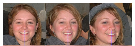
Figure 6: Progressive growing leads to “phase” artifacts. In this example the teeth do not follow the pose but stay aligned to the camera, as indicated by the blue line.
图 6:渐进式增长导致「相位」伪影。本例中牙齿不随姿态移动,而是保持与相机对齐,蓝线标出。
Progressive growing [23] has been very successful in stabilizing high-resolution image synthesis, but it causes its own characteristic artifacts. The key issue is that the progressively grown generator appears to have a strong location preference for details; the accompanying video shows that when features like teeth or eyes should move smoothly over the image, they may instead remain stuck in place before jumping to the next preferred location. Figure 6 shows a related artifact. We believe the problem is that in progressive growing each resolution serves momentarily as the output resolution, forcing it to generate maximal frequency details, which then leads to the trained network to have excessively high frequencies in the intermediate layers, compromising shift invariance [49]. Appendix A shows an example. These issues prompt us to search for an alternative formulation that would retain the benefits of progressive growing without the drawbacks.
渐进式增长[23]在稳住高分辨率图像合成上非常成功,但也带来特有伪影。关键问题是:渐进增长的生成器对细节有强烈位置偏好;配套视频显示,牙齿或眼睛本应在图像上平滑移动时,却可能先钉在原地,再跳到下一偏好位置。图 6 给出相关伪影。我们认为,原因在于渐进增长中每一分辨率都会短暂充当输出分辨率,被迫生成最高频细节,从而使训练后的网络在中间层带有过高频率,损害平移不变性[49]。附录 A 给出示例。这些问题促使我们寻找替代形式:保留渐进增长的好处,去掉其弊端。
4.1 Alternative network architectures
4.1 替代网络结构
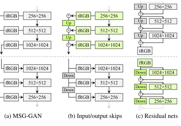
(a) MSG-GAN (b) Input/output skips (c) Residual nets
Figure 7: Three generator (above the dashed line) and discriminator architectures. Up and Down denote bilinear up and downsampling, respectively. In residual networks these also include 11 convolutions to adjust the number of feature maps. tRGB and fRGB convert between RGB and high-dimensional per-pixel data. Architectures used in configs e and f are shown in green.
(a) MSG-GAN (b) 输入/输出跳跃 (c) 残差网络
图 7:三种生成器(虚线以上)与判别器结构。Up 与 Down 分别表示双线性上/下采样。在残差网络中它们还包含 卷积以调整特征图数量。tRGB 与 fRGB 在 RGB 与高维逐像素数据之间转换。配置 e 与 f 所用结构以绿色标出。
While StyleGAN uses simple feedforward designs in the generator (synthesis network) and discriminator, there is a vast body of work dedicated to the study of better network architectures. Skip connections [34, 22], residual networks [18, 17, 31], and hierarchical methods [7, 47, 48] have proven highly successful also in the context of generative methods. As such, we decided to re-evaluate the network design of StyleGAN and search for an architecture that produces high-quality images without progressive growing.
StyleGAN 在生成器(合成网络)与判别器中使用简单前馈设计,而更好网络结构的研究文献极为丰富。跳跃连接[34, 22]、残差网络[18, 17, 31]与层次方法[7, 47, 48]在生成方法中也已被证明十分成功。因此我们决定重新评估 StyleGAN 的网络设计,寻找不依赖渐进增长仍能产出高质量图像的结构。
Figure 7a shows MSG-GAN [22], which connects the matching resolutions of the generator and discriminator using multiple skip connections. The MSG-GAN generator is modified to output a mipmap [42] instead of an image, and a similar representation is computed for each real image as well. In Figure 7b we simplify this design by upsampling and summing the contributions of RGB outputs corresponding to different resolutions. In the discriminator, we similarly provide the downsampled image to each resolution block of the discriminator. We use bilinear filtering in all up and downsampling operations. In Figure 7c we further modify the design to use residual connections.[^3] This design is similar to LAPGAN [7] without the per-resolution discriminators employed by Denton et al.
图 7a 给出 MSG-GAN [22],它用多条跳跃连接把生成器与判别器的匹配分辨率连起来。MSG-GAN 的生成器改为输出 mipmap [42] 而非单幅图像,并对每张真实图像计算类似表示。图 7b 我们简化该设计:对对应不同分辨率的 RGB 输出做上采样并求和。在判别器侧,我们同样把下采样后的图像送入每个分辨率块。所有上/下采样使用双线性滤波。图 7c 进一步改为残差连接。[^3] 该设计类似 LAPGAN [7],但不含 Denton 等人使用的按分辨率判别器。
| FFHQ | D original | D input skips | D residual | |||
|---|---|---|---|---|---|---|
| FID | PPL | FID | PPL | FID | PPL | |
| G original | 4.32 | 265 | 4.18 | 235 | 3.58 | 269 |
| G output skips | 4.33 | 169 | 3.77 | 127 | 3.31 | 125 |
| G residual | 4.35 | 203 | 3.96 | 229 | 3.79 | 243 |
| LSUN Car | D original | D input skips | D residual | |||
|---|---|---|---|---|---|---|
| FID | PPL | FID | PPL | FID | PPL | |
| G original | 3.75 | 905 | 3.23 | 758 | 3.25 | 802 |
| G output skips | 3.77 | 544 | 3.86 | 316 | 3.19 | 471 |
| G residual | 3.93 | 981 | 3.40 | 667 | 2.66 | 645 |
Table 2: Comparison of generator and discriminator architectures without progressive growing. The combination of generator with output skips and residual discriminator corresponds to configuration e in the main result table.
表 2:在无渐进增长条件下比较生成器与判别器结构。带输出跳跃的生成器与残差判别器的组合对应主结果表中的配置 e。
Table 2 compares three generator and three discriminator architectures: original feedforward networks as used in StyleGAN, skip connections, and residual networks, all trained without progressive growing. FID and PPL are provided for each of the 9 combinations. We can see two broad trends: skip connections in the generator drastically improve PPL in all configurations, and a residual discriminator network is clearly beneficial for FID. The latter is perhaps not surprising since the structure of discriminator resembles classifiers where residual architectures are known to be helpful. However, a residual architecture was harmful in the generator — the lone exception was FID in LSUN Car when both networks were residual.
表 2 比较三种生成器与三种判别器结构:StyleGAN 所用的原始前馈网络、跳跃连接与残差网络,全部在无渐进增长下训练。对 9 种组合都给出 FID 与 PPL。可见两大趋势:生成器中的跳跃连接在所有配置下都大幅改善 PPL;残差判别器对 FID 明显有利。后者或许并不意外,因为判别器结构类似分类器,而残差在分类器中已知有益。但残差结构对生成器有害——唯一例外是当两个网络都为残差时,LSUN Car 上的 FID。
For the rest of the paper we use a skip generator and a residual discriminator, without progressive growing. This corresponds to configuration e in Table 1, and it significantly improves FID and PPL.
本文后续采用带跳跃的生成器与残差判别器,且不使用渐进增长。这对应表 1 的配置 e,并显著改善 FID 与 PPL。
4.2 Resolution usage
4.2 分辨率利用率
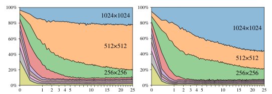
(a) StyleGAN-sized (config e) (b) Large networks (config f)
Figure 8: Contribution of each resolution to the output of the generator as a function of training time. The vertical axis shows a breakdown of the relative standard deviations of different resolutions, and the horizontal axis corresponds to training progress, measured in millions of training images shown to the discriminator. We can see that in the beginning the network focuses on low-resolution images and progressively shifts its focus on larger resolutions as training progresses. In (a) the generator basically outputs a image with some minor sharpening for , while in (b) the larger network focuses more on the high-resolution details.
(a) StyleGAN 规模(配置 e) (b) 大网络(配置 f)
图 8:各分辨率对生成器输出贡献随训练时间的变化。纵轴给出不同分辨率相对标准差的分解,横轴为训练进度,以判别器见过的训练图像百万计。可见训练初期网络聚焦低分辨率图像,随后逐步把焦点移向更高分辨率。(a) 中生成器基本上输出一幅 图像,再对 做少许锐化;而 (b) 中更大网络更关注高分辨率细节。
The key aspect of progressive growing, which we would like to preserve, is that the generator will initially focus on low-resolution features and then slowly shift its attention to finer details. The architectures in Figure 7 make it possible for the generator to first output low resolution images that are not affected by the higher-resolution layers in a significant way, and later shift the focus to the higher-resolution layers as the training proceeds. Since this is not enforced in any way, the generator will do it only if it is beneficial. To analyze the behavior in practice, we need to quantify how strongly the generator relies on particular resolutions over the course of training.
渐进增长我们希望保留的关键一点是:生成器起初聚焦低分辨率特征,再慢慢把注意力转向更细细节。图 7 中的结构使生成器可以先输出几乎不受更高分辨率层影响的低分辨率图像,随后随训练推进把焦点转移到更高分辨率层。由于这一点并未被强制,生成器只有在有益时才会这样做。为分析实际行为,我们需要量化训练过程中生成器对各分辨率的依赖强度。
Since the skip generator (Figure 7b) forms the image by explicitly summing RGB values from multiple resolutions, we can estimate the relative importance of the corresponding layers by measuring how much they contribute to the final image. In Figure 8a, we plot the standard deviation of the pixel values produced by each tRGB layer as a function of training time. We calculate the standard deviations over 1024 random samples of and normalize the values so that they sum to 100%.
由于跳跃生成器(图 7b)通过显式对多分辨率 RGB 值求和来合成图像,我们可通过测量各层对最终图像的贡献来估计相应层的相对重要性。图 8a 画出每个 tRGB 层产生像素值的标准差随训练时间的变化。我们对 1024 个随机 样本计算标准差,并归一化使其总和为 100%。
At the start of training, we can see that the new skip generator behaves similar to progressive growing — now achieved without changing the network topology. It would thus be reasonable to expect the highest resolution to dominate towards the end of the training. The plot, however, shows that this fails to happen in practice, which indicates that the generator may not be able to “fully utilize” the target resolution. To verify this, we inspected the generated images manually and noticed that they generally lack some of the pixel-level detail that is present in the training data — the images could be described as being sharpened versions of images instead of true images.
训练开始时,新的跳跃生成器行为类似渐进增长——如今无需改动网络拓扑即可达到。因此合理预期最高分辨率应在训练后期占据主导。但图中显示实践中并未发生,这表明生成器可能未能「充分利用」目标分辨率。为验证,我们人工检查生成图像,发现它们普遍缺少训练数据中的部分像素级细节——可以说更像是锐化过的 图像,而非真正的 图像。
This leads us to hypothesize that there is a capacity problem in our networks, which we test by doubling the number of feature maps in the highest-resolution layers of both networks.[^4] This brings the behavior more in line with expectations: Figure 8b shows a significant increase in the contribution of the highest-resolution layers, and Table 1, row f shows that FID and Recall improve markedly. The last row shows that baseline StyleGAN also benefits from additional capacity, but its quality remains far below StyleGAN2.
这使我们假设网络存在容量问题;通过把两个网络最高分辨率层的特征图数量加倍来检验。[^4] 行为由此更接近预期:图 8b 显示最高分辨率层贡献显著增加,表 1 行 f 显示 FID 与 Recall 明显改善。最后一行表明基线 StyleGAN 也受益于额外容量,但其质量仍远低于 StyleGAN2。
| Dataset | Resolution | StyleGAN (a) | StyleGAN2 (f) | ||
|---|---|---|---|---|---|
| FID | PPL | FID | PPL | ||
| LSUN Car | 512384 | 3.27 | 1485 | 2.32 | 416 |
| LSUN Cat | 256256 | 8.53 | 0924 | 6.93 | 439 |
| LSUN Church | 256256 | 4.21 | 0742 | 3.86 | 342 |
| LSUN Horse | 256256 | 3.83 | 1405 | 3.43 | 338 |
Table 3: Improvement in LSUN datasets measured using FID and PPL. We trained Car for 57M images, Cat for 88M, Church for 48M, and Horse for 100M images.
表 3:用 FID 与 PPL 衡量的 LSUN 数据集改进。Car 训练 57M 图像,Cat 88M,Church 48M,Horse 100M。
Table 3 compares StyleGAN and StyleGAN2 in four LSUN categories, again showing clear improvements in FID and significant advances in PPL. It is possible that further increases in the size could provide additional benefits.
表 3 在四个 LSUN 类别上比较 StyleGAN 与 StyleGAN2,再次显示 FID 的清晰改进与 PPL 的显著提升。进一步增大规模仍可能带来额外收益。
5 Projection of images to latent space
5 图像到潜空间的投影
Inverting the synthesis network is an interesting problem that has many applications. Manipulating a given image in the latent feature space requires finding a matching latent code for it first. Previous research [1, 10] suggests that instead of finding a common latent code , the results improve if a separate is chosen for each layer of the generator. The same approach was used in an early encoder implementation [32]. While extending the latent space in this fashion finds a closer match to a given image, it also enables projecting arbitrary images that should have no latent representation. Instead, we concentrate on finding latent codes in the original, unextended latent space, as these correspond to images that the generator could have produced.
对合成网络 求逆是一个有诸多应用的有趣问题。要在潜特征空间中操纵给定图像,首先需要为其找到匹配的潜码 。先前研究[1, 10]表明,与寻找共用潜码 相比,若为生成器每一层选择单独的 ,结果更好。早期编码器实现也采用同一做法[32]。如此扩展潜空间虽能更贴近给定图像,但也使本不应有潜表示的任意图像得以投影进去。我们转而专注于在原始、未扩展的潜空间中寻找潜码,因为它们对应生成器本可产出的图像。

StyleGAN — generated images StyleGAN2 — generated images StyleGAN2 — real images
Figure 9: Example images and their projected and re-synthesized counterparts. For each configuration, top row shows the target images and bottom row shows the synthesis of the corresponding projected latent vector and noise inputs. With the baseline StyleGAN, projection often finds a reasonably close match for generated images, but especially the backgrounds differ from the originals. The images generated using StyleGAN2 can be projected almost perfectly back into generator inputs, while projected real images (from the training set) show clear differences to the originals, as expected. All tests were done using the same projection method and hyperparameters.
StyleGAN — 生成图像 StyleGAN2 — 生成图像 StyleGAN2 — 真实图像
图 9:示例图像及其投影后再合成的对应结果。每种配置中,上行是目标图像,下行是对应投影潜向量与噪声输入的合成。对基线 StyleGAN,投影常能为生成图像找到尚可的匹配,但背景尤其与原图有别。StyleGAN2 生成的图像几乎可完美投影回生成器输入;而投影真实图像(来自训练集)与原图有明显差异,符合预期。所有测试使用同一投影方法与超参数。
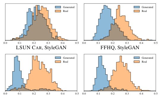
LSUN Car, StyleGAN FFHQ, StyleGAN
LSUN Car, StyleGAN2 FFHQ, StyleGAN2
Figure 10: LPIPS distance histograms between original and projected images for generated (blue) and real images (orange). Despite the higher image quality of our improved generator, it is much easier to project the generated images into its latent space . The same projection method was used in all cases.
LSUN Car, StyleGAN FFHQ, StyleGAN
LSUN Car, StyleGAN2 FFHQ, StyleGAN2
图 10:生成图像(蓝)与真实图像(橙)上,原图与投影图像之间的 LPIPS 距离直方图。尽管改进后的生成器画质更高,把生成图像投影到其潜空间 却容易得多。所有情形使用同一投影方法。
Our projection method differs from previous methods in two ways. First, we add ramped-down noise to the latent code during optimization in order to explore the latent space more comprehensively. Second, we also optimize the stochastic noise inputs of the StyleGAN generator, regularizing them to ensure they do not end up carrying coherent signal. The regularization is based on enforcing the autocorrelation coefficients of the noise maps to match those of unit Gaussian noise over multiple scales. Details of our projection method can be found in Appendix D.
我们的投影方法与先前方法有两点不同。第一,优化过程中向潜码加入逐渐衰减的噪声,以便更全面地探索潜空间。第二,我们也优化 StyleGAN 生成器的随机噪声输入,并对其正则,确保它们不会最终承载相干信号。该正则基于强制噪声图在多个尺度上的自相关系数与单位高斯噪声一致。投影方法细节见附录 D。
5.1 Attribution of generated images
5.1 生成图像的归因
Detection of manipulated or generated images is a very important task. At present, classifier-based methods can quite reliably detect generated images, regardless of their exact origin [29, 45, 40, 51, 41]. However, given the rapid pace of progress in generative methods, this may not be a lasting situation. Besides general detection of fake images, we may also consider a more limited form of the problem: being able to attribute a fake image to its specific source [2]. With StyleGAN, this amounts to checking if there exists a that re-synthesis the image in question.
检测被操纵或生成的图像非常重要。目前,基于分类器的方法已能相当可靠地检出生成图像,而无论其具体来源[29, 45, 40, 51, 41]。但生成方法进步极快,这一局面未必持久。除一般性的假图检测外,我们也可考虑更受限的形式:能否把假图归因到其具体来源[2]。对 StyleGAN 而言,这等价于检查是否存在 能重新合成所讨论的图像。
We measure how well the projection succeeds by computing the LPIPS [50] distance between original and re-synthesized image as , where is the image being analyzed and denotes the approximate projection operation. Figure 10 shows histograms of these distances for LSUN Car and FFHQ datasets using the original StyleGAN and StyleGAN2, and Figure 9 shows example projections. The images generated using StyleGAN2 can be projected into so well that they can be almost unambiguously attributed to the generating network. However, with the original StyleGAN, even though it should technically be possible to find a matching latent code, it appears that the mapping from to images is too complex for this to succeed reliably in practice. We find it encouraging that StyleGAN2 makes source attribution easier even though the image quality has improved significantly.
我们用原图与再合成图像之间的 LPIPS [50] 距离 衡量投影成功程度,其中 是被分析图像, 表示近似投影操作。图 10 给出 LSUN Car 与 FFHQ 上原始 StyleGAN 与 StyleGAN2 的这些距离直方图,图 9 给出投影示例。StyleGAN2 生成的图像可如此好地投影到 ,几乎可以毫不含糊地归因到生成网络。而对原始 StyleGAN,尽管理论上应能找到匹配潜码,但从 到图像的映射似乎过于复杂,实践中难以可靠成功。令人鼓舞的是,即便画质显著提升,StyleGAN2 仍使来源归因更容易。
6 Conclusions and future work
6 结论与未来工作
We have identified and fixed several image quality issues in StyleGAN, improving the quality further and considerably advancing the state of the art in several datasets. In some cases the improvements are more clearly seen in motion, as demonstrated in the accompanying video. Appendix A includes further examples of results obtainable using our method. Despite the improved quality, StyleGAN2 makes it easier to attribute a generated image to its source.
我们识别并修复了 StyleGAN 中若干画质问题,进一步提升质量,并在多个数据集上显著推进了当时最优水平。有些改进在运动中更清晰可见,见配套视频。附录 A 给出用我们方法可获得的更多结果示例。尽管质量提升,StyleGAN2 反而更容易把生成图像归因到其来源。
Training performance has also improved. At resolution, the original StyleGAN (config a in Table 1) trains at 37 images per second on NVIDIA DGX-1 with 8 Tesla V100 GPUs, while our config e trains 40% faster at 61 img/s. Most of the speedup comes from simplified dataflow due to weight demodulation, lazy regularization, and code optimizations. StyleGAN2 (config f, larger networks) trains at 31 img/s, and is thus only slightly more expensive to train than original StyleGAN. Its total training time was 9 days for FFHQ and 13 days for LSUN Car.
训练性能也有提升。在 分辨率上,原始 StyleGAN(表 1 配置 a)在配备 8 块 Tesla V100 的 NVIDIA DGX-1 上达到每秒 37 张图像;我们的配置 e 快约 40%,达到 61 img/s。加速主要来自权解调带来的数据流简化、惰性正则以及代码优化。StyleGAN2(配置 f,更大网络)训练速度为 31 img/s,因而只比原始 StyleGAN 略贵。其总训练时间为 FFHQ 9 天、LSUN Car 13 天。
The entire project, including all exploration, consumed 132 MWh of electricity, of which 0.68 MWh went into training the final FFHQ model. In total, we used about 51 single-GPU years of computation (Volta class GPU). A more detailed discussion is available in Appendix F.
整个项目(含全部探索)耗电 132 MWh,其中 0.68 MWh 用于训练最终 FFHQ 模型。总计约使用 51 个单 GPU 年的计算量(Volta 级 GPU)。更详细讨论见附录 F。
In the future, it could be fruitful to study further improvements to the path length regularization, e.g., by replacing the pixel-space distance with a data-driven feature-space metric. Considering the practical deployment of GANs, we feel that it will be important to find new ways to reduce the training data requirements. This is especially crucial in applications where it is infeasible to acquire tens of thousands of training samples, and with datasets that include a lot of intrinsic variation.
未来可进一步研究路径长度正则的改进,例如用数据驱动的特征空间度量替换像素空间 距离。考虑到 GAN 的实际部署,我们认为寻找降低训练数据需求的新途径很重要。这在难以获得数万训练样本的应用中尤为关键,也适用于内在变异很大的数据集。
Acknowledgements
We thank Ming-Yu Liu for an early review, Timo Viitanen for help with the public release, David Luebke for in-depth discussions and helpful comments, and Tero Kuosmanen for technical support with the compute infrastructure.
致谢
感谢 Ming-Yu Liu 的早期审阅,Timo Viitanen 协助公开发布,David Luebke 的深入讨论与有益意见,以及 Tero Kuosmanen 对计算基础设施的技术支持。
References
参考文献
[1] Rameen Abdal, Yipeng Qin, and Peter Wonka. Image2StyleGAN: How to embed images into the StyleGAN latent space? In ICCV , 2019.
[2] Michael Albright and Scott McCloskey. Source generator attribution via inversion. In CVPR Workshops , 2019.
[3] Carl Bergstrom and Jevin West. Which face is real? http://www.whichfaceisreal.com/learn.html, Accessed November 15, 2019.
[4] Christopher M. Bishop. Pattern Recognition and Machine Learning . Springer, 2006.
[5] Andrew Brock, Jeff Donahue, and Karen Simonyan. Large scale GAN training for high fidelity natural image synthesis. CoRR , abs/1809.11096, 2018.
[6] Yann N. Dauphin, Harm de Vries, and Yoshua Bengio. Equilibrated adaptive learning rates for non-convex optimization. CoRR , abs/1502.04390, 2015.
[7] Emily L. Denton, Soumith Chintala, Arthur Szlam, and Robert Fergus. Deep generative image models using a Laplacian pyramid of adversarial networks. CoRR , abs/1506.05751, 2015.
[8] Vincent Dumoulin, Ethan Perez, Nathan Schucher, Florian Strub, Harm de Vries, Aaron Courville, and Yoshua Bengio. Feature-wise transformations. Distill , 2018. https://distill.pub/2018/feature-wise-transformations.
[9] Vincent Dumoulin, Jonathon Shlens, and Manjunath Kudlur. A learned representation for artistic style. CoRR , abs/1610.07629, 2016.
[10] Aviv Gabbay and Yedid Hoshen. Style generator inversion for image enhancement and animation. CoRR , abs/1906.11880, 2019.
[11] R. Ge, X. Feng, H. Pyla, K. Cameron, and W. Feng. Power measurement tutorial for the Green500 list. https://www.top500.org/green500/resources/tutorials/, Accessed March 1, 2020.
[12] Robert Geirhos, Patricia Rubisch, Claudio Michaelis, Matthias Bethge, Felix A. Wichmann, and Wieland Brendel. ImageNet-trained CNNs are biased towards texture; increasing shape bias improves accuracy and robustness. CoRR , abs/1811.12231, 2018.
[13] Golnaz Ghiasi, Honglak Lee, Manjunath Kudlur, Vincent Dumoulin, and Jonathon Shlens. Exploring the structure of a real-time, arbitrary neural artistic stylization network. CoRR , abs/1705.06830, 2017.
[14] Xavier Glorot and Yoshua Bengio. Understanding the difficulty of training deep feedforward neural networks. In Proceedings of the Thirteenth International Conference on Artificial Intelligence and Statistics , pages 249–256, 2010.
[15] G.H. Golub and C.F. Van Loan. Matrix Computations . Johns Hopkins Studies in the Mathematical Sciences. Johns Hopkins University Press, 2013.
[16] Ian Goodfellow, Jean Pouget-Abadie, Mehdi Mirza, Bing Xu, David Warde-Farley, Sherjil Ozair, Aaron Courville, and Yoshua Bengio. Generative adversarial networks. In NIPS , 2014.
[17] Ishaan Gulrajani, Faruk Ahmed, Martín Arjovsky, Vincent Dumoulin, and Aaron C. Courville. Improved training of Wasserstein GANs. CoRR , abs/1704.00028, 2017.
[18] Kaiming He, Xiangyu Zhang, Shaoqing Ren, and Jian Sun. Deep residual learning for image recognition. CoRR , abs/1512.03385, 2015.
[19] Kaiming He, Xiangyu Zhang, Shaoqing Ren, and Jian Sun. Delving deep into rectifiers: Surpassing human-level performance on ImageNet classification. CoRR , abs/1502.01852, 2015.
[20] Martin Heusel, Hubert Ramsauer, Thomas Unterthiner, Bernhard Nessler, and Sepp Hochreiter. GANs trained by a two time-scale update rule converge to a local Nash equilibrium. In Proc. NIPS , pages 6626–6637, 2017.
[21] Xun Huang and Serge J. Belongie. Arbitrary style transfer in real-time with adaptive instance normalization. CoRR , abs/1703.06868, 2017.
[22] Animesh Karnewar and Oliver Wang. MSG-GAN: multi-scale gradients for generative adversarial networks. In Proc. CVPR , 2020.
[23] Tero Karras, Timo Aila, Samuli Laine, and Jaakko Lehtinen. Progressive growing of GANs for improved quality, stability, and variation. CoRR , abs/1710.10196, 2017.
[24] Tero Karras, Samuli Laine, and Timo Aila. A style-based generator architecture for generative adversarial networks. In Proc. CVPR , 2018.
[25] Diederik P. Kingma and Jimmy Ba. Adam: A method for stochastic optimization. In ICLR , 2015.
[26] Alex Krizhevsky, Ilya Sutskever, and Geoffrey E. Hinton. ImageNet classification with deep convolutional neural networks. In NIPS , pages 1097–1105. 2012.
[27] Tuomas Kynkäänniemi, Tero Karras, Samuli Laine, Jaakko Lehtinen, and Timo Aila. Improved precision and recall metric for assessing generative models. In Proc. NeurIPS , 2019.
[28] Barbara Landau, Linda B. Smith, and Susan S. Jones. The importance of shape in early lexical learning. Cognitive Development , 3(3), 1988.
[29] Haodong Li, Han Chen, Bin Li, and Shunquan Tan. Can forensic detectors identify GAN generated images? In Proc. Asia-Pacific Signal and Information Processing Association Annual Summit and Conference (APSIPA ASC) , 2018.
[30] Lars Mescheder, Andreas Geiger, and Sebastian Nowozin. Which training methods for GANs do actually converge? CoRR , abs/1801.04406, 2018.
[31] Takeru Miyato, Toshiki Kataoka, Masanori Koyama, and Yuichi Yoshida. Spectral normalization for generative adversarial networks. CoRR , abs/1802.05957, 2018.
[32] Dmitry Nikitko. StyleGAN – Encoder for official TensorFlow implementation. https://github.com/Puzer/stylegan-encoder/, 2019.
[33] Augustus Odena, Jacob Buckman, Catherine Olsson, Tom B. Brown, Christopher Olah, Colin Raffel, and Ian Goodfellow. Is generator conditioning causally related to GAN performance? CoRR , abs/1802.08768, 2018.
[34] Olaf Ronneberger, Philipp Fischer, and Thomas Brox. U-Net: Convolutional networks for biomedical image segmentation. In Proc. Medical Image Computing and Computer-Assisted Intervention (MICCAI) , pages 234–241, 2015.
[35] Olga Russakovsky, Jia Deng, Hao Su, Jonathan Krause, Sanjeev Satheesh, Sean Ma, Zhiheng Huang, Andrej Karpathy, Aditya Khosla, Michael S. Bernstein, Alexander C. Berg, and Fei-Fei Li. ImageNet large scale visual recognition challenge. In Proc. CVPR , 2015.
[36] Mehdi S. M. Sajjadi, Olivier Bachem, Mario Lucic, Olivier Bousquet, and Sylvain Gelly. Assessing generative models via precision and recall. CoRR , abs/1806.00035, 2018.
[37] Tim Salimans and Diederik P. Kingma. Weight normalization: A simple reparameterization to accelerate training of deep neural networks. CoRR , abs/1602.07868, 2016.
[38] Yujun Shen, Jinjin Gu, Xiaoou Tang, and Bolei Zhou. Interpreting the latent space of GANs for semantic face editing. CoRR , abs/1907.10786, 2019.
[39] Karen Simonyan and Andrew Zisserman. Very deep convolutional networks for large-scale image recognition. CoRR , abs/1409.1556, 2014.
[40] Run Wang, Lei Ma, Felix Juefei-Xu, Xiaofei Xie, Jian Wang, and Yang Liu. FakeSpotter: A simple baseline for spotting AI-synthesized fake faces. CoRR , abs/1909.06122, 2019.
[41] Sheng-Yu Wang, Oliver Wang, Richard Zhang, Andrew Owens, and Alexei A. Efros. CNN-generated images are surprisingly easy to spot… for now. CoRR , abs/1912.11035, 2019.
[42] Lance Williams. Pyramidal parametrics. SIGGRAPH Comput. Graph. , 17(3):1–11, 1983.
[43] Sitao Xiang and Hao Li. On the effects of batch and weight normalization in generative adversarial networks. CoRR , abs/1704.03971, 2017.
[44] Fisher Yu, Yinda Zhang, Shuran Song, Ari Seff, and Jianxiong Xiao. LSUN: Construction of a large-scale image dataset using deep learning with humans in the loop. CoRR , abs/1506.03365, 2015.
[45] Ning Yu, Larry Davis, and Mario Fritz. Attributing fake images to GANs: Analyzing fingerprints in generated images. CoRR , abs/1811.08180, 2018.
[46] Han Zhang, Ian Goodfellow, Dimitris Metaxas, and Augustus Odena. Self-attention generative adversarial networks. CoRR , abs/1805.08318, 2018.
[47] Han Zhang, Tao Xu, Hongsheng Li, Shaoting Zhang, Xiaolei Huang, Xiaogang Wang, and Dimitris N. Metaxas. StackGAN: text to photo-realistic image synthesis with stacked generative adversarial networks. In ICCV , 2017.
[48] Han Zhang, Tao Xu, Hongsheng Li, Shaoting Zhang, Xiaogang Wang, Xiaolei Huang, and Dimitris N. Metaxas. StackGAN++: realistic image synthesis with stacked generative adversarial networks. CoRR , abs/1710.10916, 2017.
[49] Richard Zhang. Making convolutional networks shift-invariant again. In Proc. ICML , 2019.
[50] Richard Zhang, Phillip Isola, Alexei A. Efros, Eli Shechtman, and Oliver Wang. The unreasonable effectiveness of deep features as a perceptual metric. In Proc. CVPR , 2018.
[51] Xu Zhang, Svebor Karaman, and Shih-Fu Chang. Detecting and simulating artifacts in GAN fake images. CoRR , abs/1907.06515, 2019.
Appendix A Image quality
附录 A 图像质量
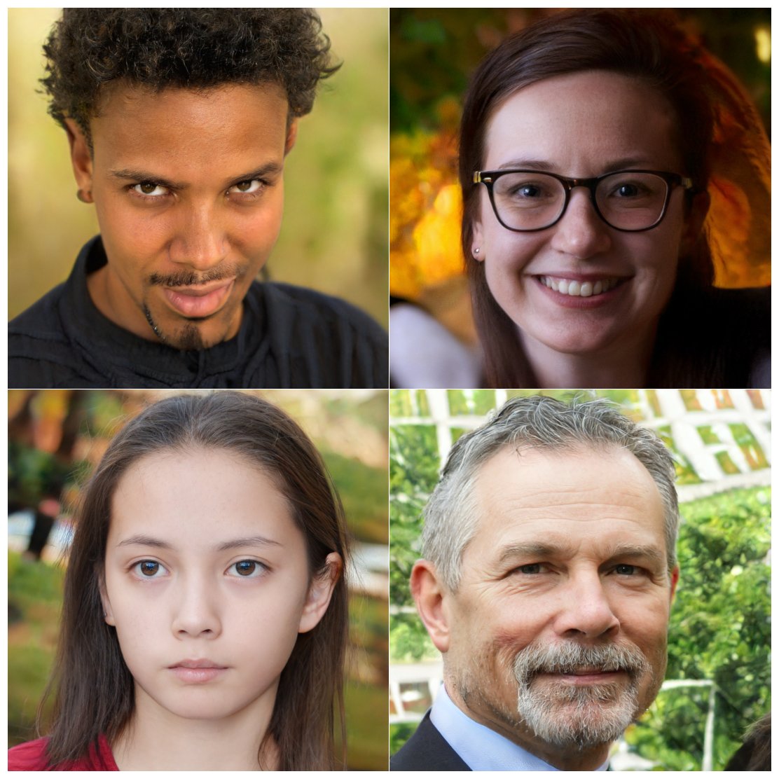
Figure 11: Four hand-picked examples illustrating the image quality and diversity achievable using StylegGAN2 (config f).
图 11:四个精选示例,展示 StyleGAN2(配置 f)可达的图像质量与多样性。
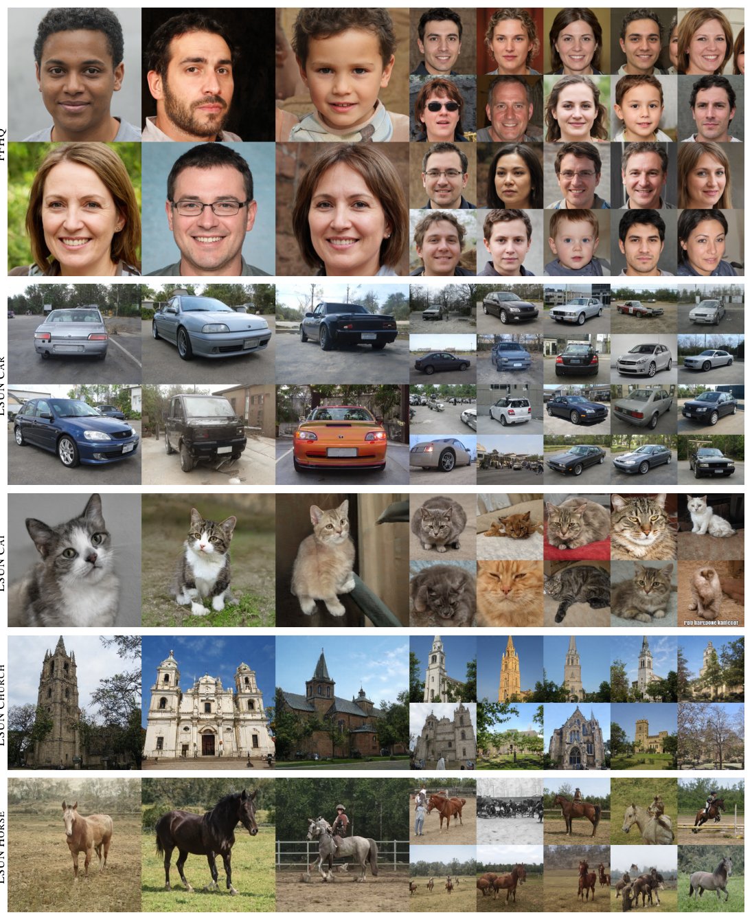
FFHQ
LSUN Car
LSUN Cat
LSUN Church
LSUN Horse
Figure 12: Uncurated results for each dataset used in Tables 1 and 3. The images correspond to random outputs produced by our generator (config f), with truncation applied at all resolutions using [24].
FFHQ
LSUN Car
LSUN Cat
LSUN Church
LSUN Horse
图 12:表 1 与表 3 所用各数据集的未筛选结果。图像对应我们生成器(配置 f)的随机输出,并在所有分辨率上以 施加截断[24]。
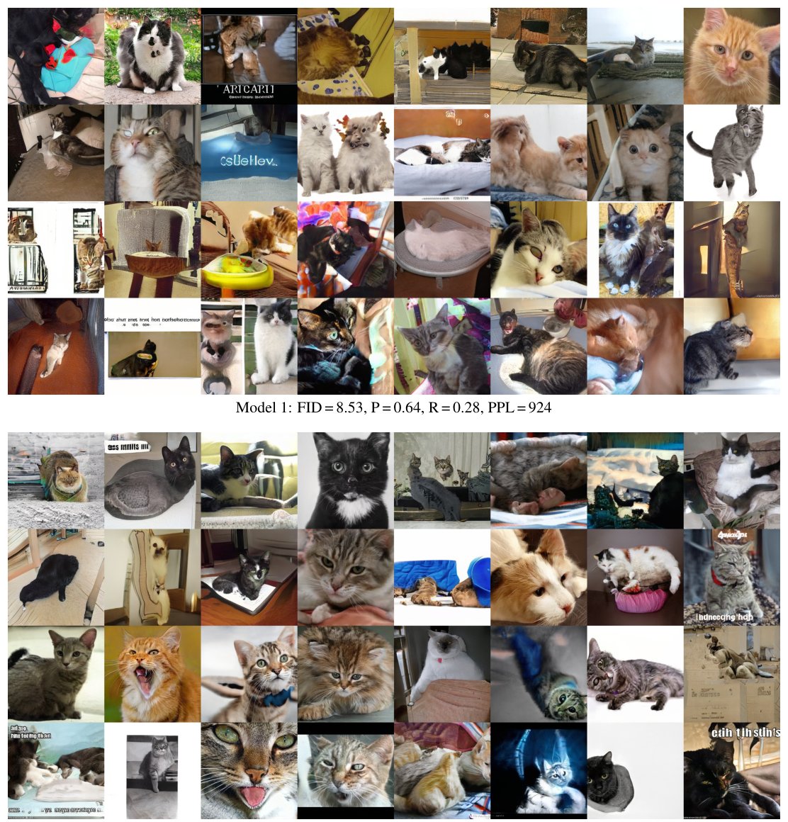
Model 1: FID = 8.53, P = 0.64, R = 0.28, PPL = 924 Model 2: FID = 8.53, P = 0.62, R = 0.29, PPL = 387
Figure 13: Uncurated examples from two generative models trained on LSUN Cat without truncation. FID, precision, and recall are similar for models 1 and 2, even though the latter produces cat-shaped objects more often. Perceptual path length (PPL) indicates a clear preference for model 2. Model 1 corresponds to configuration a in Table 3, and model 2 is an early training snapshot of configuration f.
模型 1:FID = 8.53,P = 0.64,R = 0.28,PPL = 924 模型 2:FID = 8.53,P = 0.62,R = 0.29,PPL = 387
图 13:在 LSUN Cat 上、无截断训练的两个生成模型的未筛选样例。模型 1 与 2 的 FID、精度与召回相近,但后者更常产出猫形物体。感知路径长度(PPL)明显偏好模型 2。模型 1 对应表 3 配置 a,模型 2 是配置 f 的早期训练快照。
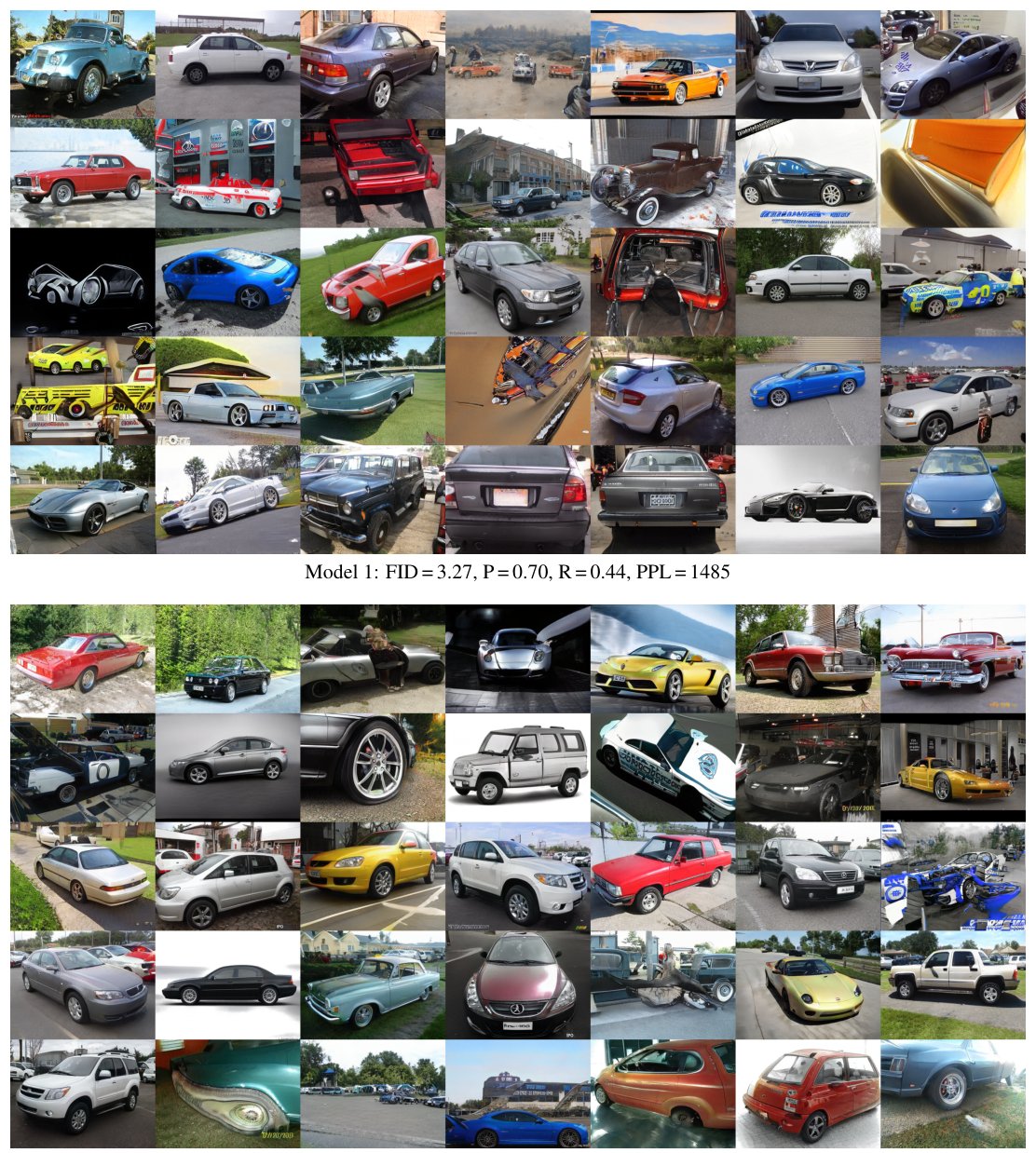
Model 1: FID = 3.27, P = 0.70, R = 0.44, PPL = 1485 Model 2: FID = 3.27, P = 0.67, R = 0.48, PPL = 437
Figure 14: Uncurated examples from two generative models trained on LSUN Car without truncation. FID, precision, and recall are similar for models 1 and 2, even though the latter produces car-shaped objects more often. Perceptual path length (PPL) indicates a clear preference for model 2. Model 1 corresponds to configuration a in Table 3, and model 2 is an early training snapshot of configuration f.
模型 1:FID = 3.27,P = 0.70,R = 0.44,PPL = 1485 模型 2:FID = 3.27,P = 0.67,R = 0.48,PPL = 437
图 14:在 LSUN Car 上、无截断训练的两个生成模型的未筛选样例。模型 1 与 2 的 FID、精度与召回相近,但后者更常产出车形物体。感知路径长度(PPL)明显偏好模型 2。模型 1 对应表 3 配置 a,模型 2 是配置 f 的早期训练快照。
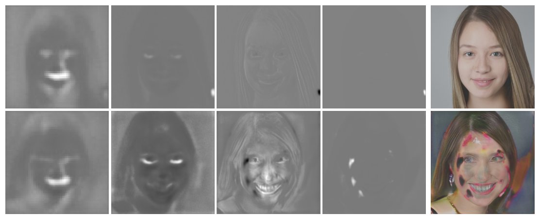
Feature map Feature map Feature map Feature map Generated image
Figure 15: An example of the importance of the droplet artifact in StyleGAN generator. We compare two generated images, one successful and one severely corrupted. The corresponding feature maps were normalized to the viewable dynamic range using instance normalization. For the top image, the droplet artifact starts forming in resolution, is clearly visible in , and increasingly dominates the feature maps in higher resolutions. For the bottom image, is qualitatively similar to the top row, but the droplet does not materialize in . Consequently, the facial features are stronger in the normalized feature map. This leads to an overshoot in , followed by multiple spurious droplets forming in subsequent resolutions. Based on our experience, it is rare that the droplet is missing from StyleGAN images, and indeed the generator fully relies on its existence.
特征图 特征图 特征图 特征图 生成图像
图 15:水滴伪影在 StyleGAN 生成器中重要性的一例。我们比较两张生成图像:一张成功,一张严重损坏。对应特征图用实例归一化压到可显示动态范围。对上行图像,水滴伪影从 开始形成,在 清晰可见,并在更高分辨率上日益支配特征图。对下行图像, 与上行定性相似,但水滴未在 出现。于是归一化后的特征图中面部特征更强,导致 过冲,随后多个虚假水滴在后续分辨率形成。按我们的经验,StyleGAN 图像中缺少水滴很少见,生成器确实完全依赖其存在。
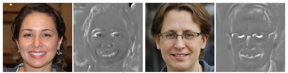
Generated image Feature map Generated image Feature map
(a) Progressive growing (config a) (b) Without progressive growing (config f)
Figure 16: Progressive growing leads to significantly higher frequency content in the intermediate layers. This compromises shift-invariance of the network and makes it harder to localize features precisely in the higher-resolution layers.
生成图像 特征图 生成图像 特征图
(a) 渐进增长(配置 a) (b) 无渐进增长(配置 f)
图 16:渐进增长导致中间层频率内容显著更高。这损害网络的平移不变性,并使更高分辨率层更难精确定位特征。
We include several large images that illustrate various aspects related to image quality. Figure 11 shows hand-picked examples illustrating the quality and diversity achievable using our method in FFHQ, while Figure 12 shows uncurated results for all datasets mentioned in the paper.
我们附上若干大幅图像,以说明与画质相关的各方面。图 11 给出精选示例,展示我们方法在 FFHQ 上可达的质量与多样性;图 12 给出文中所有数据集的未筛选结果。
Figures 13 and 14 demonstrate cases where FID and P&R give non-intuitive results, but PPL seems to be more in line with human judgement.
图 13 与图 14 展示 FID 与 P&R 给出非直观结果、但 PPL 更贴近人类判断的情形。
We also include images relating to StyleGAN artifacts. Figure 15 shows a rare case where the blob artifact fails to appear in StyleGAN activations, leading to a seriously broken image. Figure 16 visualizes the activations inside Table 1 configurations a and f. It is evident that progressive growing leads to higher-frequency content in the intermediate layers, compromising shift invariance of the network. We hypothesize that this causes the observed uneven location preference for details when progressive growing is used.
我们也附上与 StyleGAN 伪影相关的图像。图 15 给出水滴伪影未在 StyleGAN 激活中出现、从而导致严重破损图像的罕见情形。图 16 可视化表 1 配置 a 与 f 的内部激活。可见渐进增长导致中间层更高频内容,损害网络平移不变性。我们假设这造成了使用渐进增长时细节位置偏好不均匀的现象。
Appendix B Implementation details
附录 B 实现细节
We implemented our techniques on top of the official TensorFlow implementation of StyleGAN[^5] corresponding to configuration a in Table 1. We kept most of the details unchanged, including the dimensionality of and (512), mapping network architecture (8 fully connected layers, 100 lower learning rate), equalized learning rate for all trainable parameters [23], leaky ReLU activation with , bilinear filtering [49] in all up/downsampling layers [24], minibatch standard deviation layer at the end of the discriminator [23], exponential moving average of generator weights [23], style mixing regularization [24], non-saturating logistic loss [16] with regularization [30], Adam optimizer [25] with the same hyperparameters (), and training datasets [24, 44]. We performed all training runs on NVIDIA DGX-1 with 8 Tesla V100 GPUs using TensorFlow 1.14.0 and cuDNN 7.4.2.
我们在 StyleGAN 官方 TensorFlow 实现[^5]之上实现各项技术,对应表 1 配置 a。多数细节保持不变,包括 与 的维度(512)、映射网络结构(8 个全连接层,学习率低 )、所有可训练参数的均衡学习率[23]、 的 leaky ReLU、所有上/下采样层中的双线性滤波[49, 24]、判别器末端的 minibatch 标准差层[23]、生成器权重的指数滑动平均[23]、风格混合正则[24]、带 正则[30]的非饱和 logistic 损失[16]、超参数相同的 Adam 优化器[25]()以及训练数据集[24, 44]。全部训练在配备 8 块 Tesla V100 的 NVIDIA DGX-1 上运行,使用 TensorFlow 1.14.0 与 cuDNN 7.4.2。
Generator redesign
In configurations b–f we replace the original StyleGAN generator with our revised architecture. In addition to the changes highlighted in Section 2, we initialize components of the constant input using and simplify the noise broadcast operations to use a single shared scaling factor for all feature maps. Similar to Karras et al. [24], we initialize all weights using and all biases and noise scaling factors to zero, except for the biases of the affine transformation layers, which we initialize to one. We employ weight modulation and demodulation in all convolution layers, except for the output layers (tRGB in Figure 7) where we leave out the demodulation. With output resolution, the generator contains a total of 18 affine transformation layers where the first one corresponds to resolution, the next two correspond to , and so forth.
生成器重设计
在配置 b–f 中,我们用修订后的结构替换原始 StyleGAN 生成器。除第 2 节强调的改动外,我们用 初始化常数输入 的分量,并把噪声广播简化为对所有特征图使用单一共享缩放因子。与 Karras 等人[24]类似,所有权重用 初始化,所有偏置与噪声缩放因子初始化为零,仿射变换层的偏置除外(初始化为 1)。我们在所有卷积层采用权调制与解调,输出层(图 7 中的 tRGB)除外,后者去掉解调。在 输出分辨率下,生成器共有 18 个仿射变换层:第一个对应 ,随后两个对应 ,以此类推。
Weight demodulation
Considering the practical implementation of Equations 1 and 3, it is important to note that the resulting set of weights will be different for each sample in a minibatch, which rules out direct implementation using standard convolution primitives. Instead, we choose to employ grouped convolutions [26] that were originally proposed as a way to reduce computational costs by dividing the input feature maps into multiple independent groups, each with their own dedicated set of weights. We implement Equations 1 and 3 by temporarily reshaping the weights and activations so that each convolution sees one sample with groups — instead of samples with one group. This approach is highly efficient because the reshaping operations do not actually modify the contents of the weight and activation tensors.
权解调
考虑式 1 与式 3 的实际实现时,重要的是:所得权重集合对 minibatch 中每个样本都不同,从而排除用标准卷积原语直接实现。我们转而采用分组卷积[26]——最初提出是为了把输入特征图分成多个独立组、每组有专用权重以降低计算成本。实现式 1 与式 3 时,我们临时重塑权重与激活,使每次卷积看到的是带 个组的一个样本——而不是带一个组的 个样本。该方法高效,因为重塑并不真正修改权重与激活张量的内容。
Lazy regularization
In configurations c–f we employ lazy regularization (Section 3.1) by evaluating the regularization terms ( and path length) in a separate regularization pass that we execute once every training iterations. We share the internal state of the Adam optimizer between the main loss and the regularization terms, so that the optimizer first sees gradients from the main loss for iterations, followed by gradients from the regularization terms for one iteration. To compensate for the fact that we now perform training iterations instead of , we adjust the optimizer hyperparameters , , and , where . We also multiply the regularization term by to balance the overall magnitude of its gradients. We use for the discriminator and for the generator.
惰性正则
在配置 c–f 中,我们采用惰性正则(第 3.1 节):在单独的正则化 pass 中评估正则项( 与路径长度),每 次训练迭代执行一次。Adam 优化器的内部状态在主损失与正则项之间共享,因此优化器先连续 次见到主损失梯度,再见到一次正则项梯度。为补偿现在执行 次而非 次训练迭代,我们调整优化器超参数 ,,,其中 。我们还将正则项乘以 以平衡其梯度总体幅度。判别器取 ,生成器取 。
Path length regularization
Configurations d–f include our new path length regularizer (Section 3.2). We initialize the target scale to zero and track it on a per-GPU basis as the exponential moving average of using decay coefficient . We weight our regularization term by
路径长度正则
配置 d–f 包含我们的新路径长度正则(第 3.2 节)。我们将目标尺度 初始化为零,并按 GPU 跟踪 的指数滑动平均,衰减系数 。正则项的权重取
where specifies the output resolution (e.g. ). We have found these parameter choices to work reliably across all configurations and datasets. To ensure that our regularizer interacts correctly with style mixing regularization, we compute it as an average of all individual layers of the synthesis network. Appendix C provides detailed analysis of the effects of our regularizer on the mapping between and image space.
其中 指定输出分辨率(例如 )。我们发现这些参数选择在所有配置与数据集上都很可靠。为确保正则与风格混合正则正确交互,我们将其算作合成网络所有各层的平均。附录 C 详细分析该正则对 与图像空间之间映射的影响。
Progressive growing
In configurations a–d we use progressive growing with the same parameters as Karras et al. [24] (start at resolution and learning rate , train for 600k images per resolution, fade in next resolution for 600k images, increase learning rate gradually by ). In configurations e–f we disable progressive growing and set the learning rate to a fixed value , which we found to provide the best results. In addition, we use output skips in the generator and residual connections in the discriminator as detailed in Section 4.1.
渐进增长
配置 a–d 使用与 Karras 等人[24]相同参数的渐进增长(从 分辨率与学习率 起步,每个分辨率训练 600k 图像,下一分辨率淡入 600k 图像,学习率逐步提高 )。配置 e–f 关闭渐进增长,并将学习率固定为 ,我们发现这给出最佳结果。此外,按第 4.1 节,生成器使用输出跳跃,判别器使用残差连接。
Dataset-specific tuning
Similar to Karras et al. [24], we augment the FFHQ dataset with horizontal flips to effectively increase the number of training images from 70k to 140k, and we do not perform any augmentation for the LSUN datasets. We have found that the optimal choices for the training length and regularization weight tend to vary considerably between datasets and configurations. We use for all training runs except for configuration e in Table 1, as well as LSUN Church and LSUN Horse in Table 3, where we use . It is possible that further tuning of could provide additional benefits.
数据集相关调参
与 Karras 等人[24]类似,我们对 FFHQ 做水平翻转以有效把训练图像从 70k 增至 140k;LSUN 数据集不做任何增强。我们发现训练长度与 正则权重 的最优选择在不同数据集与配置间差异很大。除表 1 配置 e 以及表 3 的 LSUN Church 与 LSUN Horse 使用 外,其余训练运行使用 。进一步调 仍可能带来额外收益。
Performance optimizations
We profiled our training runs extensively and found that — in our case — the default primitives for image filtering, up/downsampling, bias addition, and leaky ReLU had surprisingly high overheads in terms of training time and GPU memory footprint. This motivated us to optimize these operations using hand-written CUDA kernels. We implemented filtered up/downsampling as a single fused operation, and bias and activation as another one. In configuration e at resolution, our optimizations improved the overall training time by about 30% and memory footprint by about 20%.
性能优化
我们广泛剖析训练运行,发现——就我们的情形而言——图像滤波、上/下采样、加偏置与 leaky ReLU 的默认原语在训练时间与 GPU 显存占用上开销出奇地高。这促使我们用手写 CUDA 核优化这些操作。我们把带滤波的上/下采样实现为单一融合操作,把偏置与激活实现为另一融合操作。在配置 e、 分辨率下,优化使总体训练时间约改善 30%,显存占用约改善 20%。
Appendix C Effects of path length regularization
附录 C 路径长度正则的效应
The path length regularizer described in Section 3.2 is of the form:
第 3.2 节描述的路径长度正则形式为:
where is a unit normal distributed random variable in the space of generated images (of dimension , namely the RGB image dimensions), is the Jacobian matrix of the generator function at a latent space point , and is a global value that expresses the desired scale of the gradients.
其中 是生成图像空间中的单位正态随机变量(维度 ,即 RGB 图像维), 是生成器函数 在潜空间点 处的雅可比矩阵, 是表达梯度期望尺度的全局值。
C.1 Effect on pointwise Jacobians
C.1 对逐点雅可比的效应
The value of this prior is minimized when the inner expectation over is minimized at every latent space point separately. In this subsection, we show that the inner expectation is (approximately) minimized when the Jacobian matrix is orthogonal, up to a global scaling factor. The general strategy is to use the well-known fact that, in high dimensions , the density of a unit normal distribution is concentrated on a spherical shell of radius . The inner expectation is then minimized when the matrix scales the function under expectation to have its minima at this radius. This is achieved by any orthogonal matrix (with suitable global scale that is the same at every ).
当对每个潜空间点 分别最小化关于 的内层期望时,该先验取值最小。本小节表明:当雅可比矩阵 正交(至多差一个全局缩放因子)时,内层期望被(近似)最小化。总体策略是利用熟知事实:在高维 下,单位正态分布的密度集中在半径 的球壳上。于是当矩阵 把期望下的函数缩放,使其最小值落在该半径时,内层期望被最小化。任意正交矩阵(配以在每个 相同的合适全局尺度)均可达到。
We begin by considering the inner expectation
我们从内层期望入手
We first note that the radial symmetry of the distribution of , as well as of the norm, allows us to focus on diagonal matrices only. This is seen using the Singular Value Decomposition , where and are orthogonal matrices, and is a horizontal concatenation of a diagonal matrix and a zero matrix [15]. Because rotating a unit normal random variable by an orthogonal matrix leaves the distribution unchanged, and rotating a vector leaves its norm unchanged, the expression simplifies to
首先注意到, 分布的径向对称性以及 范数的性质,使我们只需关注对角矩阵。这一点可用奇异值分解 看出,其中 与 为正交矩阵, 是对角矩阵 与零矩阵 的水平拼接[15]。因为用正交矩阵旋转单位正态随机变量不改变分布,旋转向量不改变其范数,表达式简化为
Furthermore, the zero matrix in drops the dimensions of beyond , effectively marginalizing its distribution over those dimensions. The marginalized distribution is again a unit normal distribution over the remaining dimensions. We are then left to consider the minimization of the expression
此外, 中的零矩阵丢掉 超出 的维度,等价于在这些维上边缘化其分布。边缘化后的分布在剩余 维上仍是单位正态。于是我们只需考虑最小化表达式
over diagonal square matrices , where is unit normal distributed in dimension . To summarize, all matrices that share the same singular values with produce the same value for the original loss.
其中最小化在对角方阵 上进行, 是 维单位正态。总结:所有与 共享相同奇异值的矩阵 对原始损失给出相同取值。
Next, we show that this expression is minimized when the diagonal matrix has a specific identical value at every diagonal entry, i.e., it is a constant multiple of an identity matrix. We first write the expectation as an integral over the probability density of :
接下来我们证明:当对角矩阵 在每个对角元取相同特定值,亦即它是单位矩阵的常数倍时,该表达式被最小化。我们先把期望写成对 概率密度的积分:
Observing the radially symmetric form of the density, we change into a polar coordinates , where is the distance from origin, and is a unit vector, i.e., a point on the -dimensional unit sphere. This change of variables introduces a Jacobian factor :
观察到密度的径向对称形式,我们换到极坐标 ,其中 是到原点的距离, 是单位向量,即 维单位球面上的点。该变量替换引入雅可比因子 :
$$\tilde{\mathcal{L}}{{\bf w}}=(2\pi)^{-\frac{L}{2}}\int{\mathbb{S}}\int_{0}^{\infty}\left(r\left\lVert{\bf\Sigma}\phi\right\rVert_{2}-a\right)^{2}r^{L-1}\
\mathrm{exp}\left(-\frac{r^{2}}{2}\right)\mathrm{d}r\mathrm{d}\phi$$
The probability density is then an -dimensional unit normal density expressed in polar coordinates, dependent only on the radius and not on the angle. A standard argument by Taylor approximation shows that when is high, for any the density is well approximated by density , which is a (unnormalized) one-dimensional normal density in , centered at of standard deviation [4]. In other words, the density of the -dimensional unit normal distribution is concentrated on a shell of radius . Substituting this density into the integral, the loss becomes approximately
于是概率密度 是用极坐标表示的 维单位正态密度,只依赖半径而不依赖角度。用泰勒近似的标准论证表明:当 很高时,对任意 ,该密度可被密度 良好近似,后者是关于 的(未归一)一维正态密度,中心在 ,标准差 [4]。换言之, 维单位正态分布的密度集中在半径 的壳上。把该密度代入积分,损失近似成为
$$\mathcal{L}{{\bf w}}\approx(2\pi e/L)^{-L/2}\int{\mathbb{S}}\int_{0}^{\infty}\left(r\left\lVert{\bf\Sigma}\phi\right\rVert_{2}-a\right)^{2}\
\mathrm{exp}\left(-\frac{\left(r-\sqrt{L}\right)^{2}}{2\sigma^{2}}\right)\mathrm{d}r\mathrm{d}\phi, \tag{7}$$
where the approximation becomes exact in the limit of infinite dimension .
其中当维数 趋于无穷时近似变为精确。
To minimize this loss, we set such that the function obtains minimal values on the spherical shell of radius . This is achieved by , whereby the function becomes constant in and the expression reduces to
为最小化该损失,我们设定 使函数 在半径 的球壳上取最小值。这由 达到,此时函数对 为常数,表达式化为
$$\mathcal{L}{{\bf w}}\approx(2\pi e/L)^{-L/2}\mathcal{A}(\mathbb{S})a^{2}L^{-1}\int{0}^{\infty}\left(r-\sqrt{L}\right)^{2}\
\mathrm{exp}\left(-\frac{\left(r-\sqrt{L}\right)^{2}}{2\sigma^{2}}\right)~\mathrm{d}r,$$
where is the surface area of the unit sphere (and like the other constant factors, irrelevant for minimization). Note that the zero of the parabola coincides with the maximum of the probability density, and therefore this choice of minimizes the inner integral in Eq. 7 separately for every .
其中 是单位球面面积(与其他常数因子一样,对最小化无关紧要)。注意抛物线 的零点与概率密度最大值重合,因此这一 选择对每个 分别最小化式 7 中的内层积分。
In summary, we have shown that — assuming a high dimensionality of the latent space — the value of the path length prior (Eq. 6) is minimized when all singular values of the Jacobian matrix of the generator are equal to a global constant, at every latent space point , i.e., they are orthogonal up to a globally constant scale.
总结:我们已证明——在潜空间维数 较高的假设下——当生成器雅可比矩阵的所有奇异值在每个潜空间点 都等于同一全局常数时,亦即它们正交至多差一个全局常数尺度时,路径长度先验(式 6)取值最小。
While in theory merely scales the values of the mapping without changing its properties and could be set to a fixed value (e.g., ), in practice it does affect the dynamics of the training. If the imposed scale does not match the scale induced by the random initialization of the network, the training spends its critical early steps in pushing the weights towards the required overall magnitudes, rather than enforcing the actual objective of interest. This may degrade the internal state of the network weights and lead to sub-optimal performance in later training. Empirically we find that setting a fixed scale reduces the consistency of the training results across training runs and datasets. Instead, we set dynamically based on a running average of the existing scale of the Jacobians, namely . With this choice the prior targets the scale of the local Jacobians towards whatever global average already exists, rather than forcing a specific global average. This also eliminates the need to measure the appropriate scale of the Jacobians explicitly, as is done by Odena et al. [33] who consider a related conditioning prior.
理论上 只缩放映射取值而不改变其性质,可设为固定值(例如 );实践中它确实影响训练动态。若强加的尺度与网络随机初始化诱导的尺度不匹配,训练会把关键早期步骤花在把权重推向所需总体幅度上,而非执行真正关心的目标。这可能损害网络权重的内部状态,并导致后期次优性能。经验上我们发现,固定尺度会降低跨训练运行与数据集的结果一致性。我们改为根据雅可比现有尺度的滑动平均动态设定 ,即 。如此先验把局部雅可比的尺度推向已存在的全局平均,而非强制某一特定全局平均。这也消除了像 Odena 等人[33]在相关条件先验中那样显式测量雅可比合适尺度的需要。
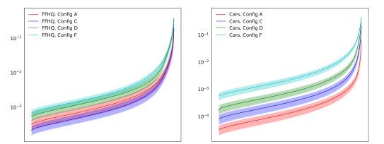
Figure 17: The mean and standard deviation of the magnitudes of sorted singular values of the Jacobian matrix evaluated at random latent space points , with largest eigenvalue normalized to . In both datasets, path length regularization (Config D) and novel architecture (Config F) exhibit better conditioning; notably, the effect is more pronounced in the Cars dataset that contains much more variability, and where path length regularization has a relatively stronger effect on the PPL metric (Table 1).
图 17:在随机潜空间点 处评估的雅可比矩阵经排序奇异值幅度的均值与标准差,最大特征值归一化为 。在两个数据集上,路径长度正则(配置 D)与新结构(配置 F)都展现更好的条件数;尤其在变异更大的 Cars 数据集上效应更明显,且路径长度正则对 PPL 指标的相对影响也更强(表 1)。
Figure 17 shows empirically measured magnitudes of singular values of the Jacobian matrix for networks trained with and without path length regularization. While orthogonality is not reached, the eigenvalues of the regularized network are closer to one another, implying better conditioning, with the strength of the effect correlated with the PPL metric (Table 1).
图 17 给出有无路径长度正则训练的网络上雅可比奇异值幅度的经验测量。虽未达到正交,但正则化网络的特征值彼此更接近,意味着条件更好,效应强度与 PPL 指标相关(表 1)。
C.2 Effect on global properties of generator mapping
C.2 对生成器映射全局性质的效应
In the previous subsection, we found that the prior encourages the Jacobians of the generator mapping to be everywhere orthogonal. While Figure 17 shows that the mapping does not satisfy this constraint exactly in practice, it is instructive to consider what global properties the constraint implies for mappings that do. Without loss of generality, we assume unit global scale for the matrices to simplify the presentation.
上一小节我们看到,先验鼓励生成器映射的雅可比处处正交。尽管图 17 显示实践中映射并未精确满足该约束,仍有必要考察:对确实满足约束的映射,它蕴含哪些全局性质。不失一般性,我们假设矩阵具有单位全局尺度以简化叙述。
The key property is that that a mapping with everywhere orthogonal Jacobians preserves the lengths of curves. To see this, let parametrize a curve in the latent space. Mapping the curve through the generator , we obtain a curve in the space of images. Its arc length is
关键性质是:雅可比处处正交的映射 保持曲线长度。为此,设 参数化潜空间中的一条曲线。经生成器 映射后,得到图像空间中的曲线 。其弧长为
where prime denotes derivative with respect to . By chain rule, this equals
其中撇号表示对 求导。由链式法则,这等于
where is the Jacobian matrix of evaluated at . By our assumption, the Jacobian is orthogonal, and consequently it leaves the 2-norm of the vector unaffected:
其中 是 在 处评估的雅可比矩阵。按假设雅可比正交,因而它不改变向量 的 2-范数:
This is the length of the curve in the latent space, prior to mapping with . Hence, the lengths of and are equal, and so preserves the length of any curve.
这正是曲线 在经 映射之前、在潜空间中的长度。因此 与 长度相等,故 保持任意曲线的长度。
In the language of differential geometry, isometrically embeds the Euclidean latent space L into a submanifold in M — e.g., the manifold of images representing faces, embedded within the space of all possible RGB images. A consequence of isometry is that straight line segments in the latent space are mapped to geodesics, or shortest paths, on the image manifold: a straight line that connects two latent space points cannot be made any shorter, so neither can there be a shorter on-manifold image-space path between the corresponding images than . For example, a geodesic on the manifold of face images is a continuous morph between two faces that incurs the minimum total amount of change (as measured by difference in RGB space) when one sums up the image difference in each step of the morph.
用微分几何的语言, 把欧氏潜空间 L 等距嵌入到 M 中的子流形 ——例如嵌入在所有可能 RGB 图像空间中的「人脸图像流形」。等距的一个后果是:潜空间中的直线段被映射为图像流形上的测地线,即最短路径:连接两个潜空间点的直线 已不能再缩短,因而对应图像之间也不存在比 更短的流形上图像空间路径。例如,人脸图像流形上的测地线是两张脸之间的连续形变,当把形变每一步的图像差(以 RGB 空间 差度量)累加时,总变化量最小。
Isometry is not achieved in practice, as demonstrated in empirical experiments in the previous subsection. The full loss function of the training is a combination of potentially conflicting criteria, and it is not clear if a genuinely isometric mapping would be capable of expressing the image manifold of interest. Nevertheless, a pressure to make the mapping as isometric as possible has desirable consequences. In particular, it discourages unnecessary “detours”: in a non-constrained generator mapping, a latent space interpolation between two similar images may pass through any number of distant images in RGB space. With regularization, the mapping is encouraged to place distant images in different regions of the latent space, so as to obtain short image paths between any two endpoints.
实践中并未达到等距,如上一小节经验实验所示。训练的完整损失函数是可能相互冲突的准则的组合,也不清楚真正等距的映射是否有能力表达所关心的图像流形。尽管如此,尽可能使映射等距的压力仍有可取后果。尤其是,它抑制不必要的「绕路」:在无约束的生成器映射中,两张相似图像之间的潜空间插值可能经过 RGB 空间中任意多张遥远图像。有了正则,映射被鼓励把遥远图像放在潜空间的不同区域,从而使任意两端点之间的图像路径更短。
Appendix D Projection method details
附录 D 投影方法细节
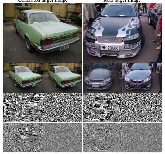
Generated target image Real target image No noise With noise No noise With noise regularization regularization regularization regularization
Figure 18: Effect of noise regularization in latent-space projection where we also optimize the contents of the noise inputs of the synthesis network. Top to bottom: target image, re-synthesized image, contents of two noise maps at different resolutions. When regularization is turned off in this test, we only normalize the noise maps to zero mean and unit variance, which leads the optimization to sneak signal into the noise maps. Enabling the noise regularization prevents this. The model used here corresponds to configuration f in Table 1.
生成目标图像 真实目标图像 无噪声正则 有噪声正则 无噪声正则 有噪声正则
图 18:潜空间投影中噪声正则的效应;我们同时优化合成网络噪声输入的内容。自上而下:目标图像、再合成图像、两个不同分辨率噪声图的内容。本测试关闭正则时,我们只把噪声图归一化到零均值单位方差,这导致优化把信号偷偷塞进噪声图。开启噪声正则可阻止这一点。此处所用模型对应表 1 配置 f。
Given a target image , we seek to find the corresponding and per-layer noise maps denoted where is the layer index and denotes the resolution of the th noise map. The baseline StyleGAN generator in 10241024 resolution has 18 noise inputs, i.e., two for each resolution from 44 to 10241024 pixels. Our improved architecture has one fewer noise input because we do not add noise to the learned 44 constant (Figure 2).
给定目标图像 ,我们寻求对应的 以及按层噪声图 ,其中 是层索引, 是第 个噪声图的分辨率。 分辨率下的基线 StyleGAN 生成器有 18 个噪声输入,即从 到 每个分辨率两个。我们改进后的结构少一个噪声输入,因为不对学到的 常数加噪声(图 2)。
Before optimization, we compute by running 10 000 random latent codes through the mapping network . We also approximate the scale of by computing , i.e., the average square Euclidean distance to the center.
优化前,我们通过把 10 000 个随机潜码 送入映射网络 计算 。我们也用 近似 的尺度,即到中心的平均平方欧氏距离。
At the beginning of optimization, we initialize and for all . The trainable parameters are the components of as well as all components in all noise maps . The optimization is run for 1000 iterations using Adam optimizer [25] with default parameters. Maximum learning rate is , and it is ramped up from zero linearly during the first 50 iterations and ramped down to zero using a cosine schedule during the last 250 iterations. In the first three quarters of the optimization we add Gaussian noise to when evaluating the loss function as , where goes from one to zero during the first 750 iterations. This adds stochasticity to the optimization and stabilizes finding of the global optimum.
优化开始时,我们初始化 ,并对所有 取 。可训练参数是 的分量以及所有噪声图 中的全部分量。优化用默认参数的 Adam 优化器[25]运行 1000 次迭代。最大学习率为 ,前 50 次迭代从零线性升高,最后 250 次用余弦日程降回零。在优化前四分之三阶段,评估损失函数时向 加入高斯噪声:,其中 在前 750 次迭代中从一降到零。这为优化加入随机性,并稳住对全局最优的寻找。
Given that we are explicitly optimizing the noise maps, we must be careful to avoid the optimization from sneaking actual signal into them. Thus we include several noise map regularization terms in our loss function, in addition to an image quality term. The image quality term is the LPIPS [50] distance between target image and the synthesized image: . For increased performance and stability, we downsample both images to 256256 resolution before computing the LPIPS distance. Regularization of the noise maps is performed on multiple resolution scales. For this purpose, we form for each noise map greater than 88 in size a pyramid down to 88 resolution by averaging 22 pixel neighborhoods and multiplying by 2 at each step to retain the expected unit variance. These downsampled noise maps are used for regularization only and have no part in synthesis.
既然我们显式优化噪声图,就必须小心避免优化把真实信号偷偷塞进去。因此除图像质量项外,损失函数中还包含若干噪声图正则项。图像质量项是目标图像 与合成图像之间的 LPIPS [50] 距离:。为提升性能与稳定性,计算 LPIPS 前我们把两幅图像都下采样到 。噪声图正则在多个分辨率尺度上进行。为此,对每个大于 的噪声图,我们通过对 像素邻域求平均并在每一步乘以 2 以保持期望单位方差,形成下至 的金字塔。这些下采样噪声图仅用于正则,不参与合成。
Let us denote the original noise maps by and the downsampled versions by . Similarly, let be the resolution of an original () or downsampled () noise map so that . The regularization term for noise map is then
记原始噪声图为 ,下采样版本为 。类似地,令 为原始()或下采样()噪声图的分辨率,使得 。则噪声图 的正则项为
where the noise map is considered to wrap at the edges. The regularization term is thus sum of squares of the resolution-normalized autocorrelation coefficients at one pixel shifts horizontally and vertically, which should be zero for a normally distributed signal. The overall loss term is then . In all our tests, we have used noise regularization weight . In addition, we renormalize all noise maps to zero mean and unit variance after each optimization step. Figure 18 illustrates the effect of noise regularization on the resulting noise maps.
其中噪声图在边缘处视为环绕。因此正则项是水平与竖直各一个像素位移处、经分辨率归一的自相关系数的平方和;对正态分布信号它们应为零。总体损失项为 。我们所有测试使用噪声正则权重 。此外,每步优化后把所有噪声图重新归一到零均值单位方差。图 18 说明噪声正则对所得噪声图的影响。
Appendix E Results with spectral normalization
附录 E 谱归一化结果
| SN-G | SN-D | Demod | P.reg | FID | PPL | Pre. | Rec. | |
|---|---|---|---|---|---|---|---|---|
| 1 | – | – | ✓ | ✓ | 2.83 | 145.0 | 0.689 | 0.492 |
| 2 | – | ✓ | ✓ | ✓ | 2.98 | 131.4 | 0.700 | 0.469 |
| 3 | ✓ | ✓ | ✓ | ✓ | 3.40 | 130.9 | 0.720 | 0.435 |
| 4 | ✓ | ✓ | – | ✓ | 3.38 | 162.6 | 0.705 | 0.468 |
| 5 | ✓ | ✓ | – | – | 3.33 | 394.9 | 0.705 | 0.463 |
| 6 | ✓ | – | – | ✓ | 3.36 | 217.1 | 0.695 | 0.464 |
| 7 | ✓ | – | – | – | 3.22 | 394.4 | 0.692 | 0.489 |
Table 4: Effect of spectral normalization with FFHQ at . The first row corresponds to StyleGAN2, i.e., config f in Table 1. In the subsequent rows, we enable spectral normalization in the generator (SN-G) and in the discriminator (SN-D). We also test the training without weight demodulation (Demod) and path length regularization (P.reg). All of these configurations are highly detrimental to FID, as well as to Recall. indicates that higher is better, and that lower is better.
表 4:在 的 FFHQ 上谱归一化的效应。第一行对应 StyleGAN2,即表 1 配置 f。随后各行在生成器(SN-G)与判别器(SN-D)中启用谱归一化。我们也测试去掉权解调(Demod)与路径长度正则(P.reg)的训练。这些配置都严重损害 FID 以及 Recall。 表示越高越好, 表示越低越好。
Since spectral normalization (SN) is widely used in GANs [31], we investigated its effect on StyleGAN2. Table 4 gives the results for a variety of configurations where spectral normalization is enabled in addition to our techniques (weight demodulation, path length regularization) or instead of them.
由于谱归一化(SN)在 GAN 中广泛使用[31],我们考察其对 StyleGAN2 的影响。表 4 给出多种配置的结果:在我们的技术(权解调、路径长度正则)之上或替代它们启用谱归一化。
Interestingly, adding spectral normalization to our generator is almost a no-op. On an implementation level, SN scales the weight tensor of each layer with a scalar value . The effect of such scaling, however, is overridden by Equation 3 for the main convolutional layers as well as the affine transformation layers. Thus, the only thing that SN adds on top of weight demodulation is through its effect on the tRGB layers.
有趣的是,在我们的生成器上加谱归一化几乎是空操作。实现层面,SN 用标量 缩放每层权重张量。然而对主卷积层以及仿射变换层,这种缩放的效果会被式 3 覆盖。因此 SN 在权解调之上唯一新增的,是通过对 tRGB 层的影响。
When we enable spectral normalization in the discriminator, FID is slightly compromised. Enabling it in the generator as well leads to significantly worse results, even though its effect is isolated to the tRGB layers. Leaving SN enabled, but disabling a subset of our contributions does not improve the situation. Thus we conclude that StyleGAN2 gives better results without spectral normalization.
在判别器启用谱归一化时,FID 略有受损。若生成器也启用,结果显著更差,即便其效应仅限于 tRGB 层。保持 SN 开启但关掉我们一部分贡献并不能改善局面。因此我们结论是:StyleGAN2 在不使用谱归一化时结果更好。
Appendix F Energy consumption
附录 F 能耗
| Item | GPU years (Volta) | Electricity (MWh) |
|---|---|---|
| Initial exploration | 20.25 | 58.94 |
| Paper exploration | 13.71 | 31.49 |
| FFHQ config f | 00.23 | 00.68 |
| Other runs in paper | 07.20 | 16.77 |
| Backup runs left out | 04.73 | 12.08 |
| Video, figures, etc. | 00.31 | 00.82 |
| Public release | 04.62 | 10.82 |
| Total | 51.05 | 131.61 |
Table 5: Computational effort expenditure and electricity consumption data for this project. The unit for computation is GPU-years on a single NVIDIA V100 GPU — it would have taken approximately 51 years to execute this project using a single GPU. See the text for additional details about the computation and energy consumption estimates. Initial exploration includes all training runs after the release of StyleGAN [24] that affected our decision to start this project. Paper exploration includes all training runs that were done specifically for this project, but were not intended to be used in the paper as-is. FFHQ config F refers to the training of the final network. This is approximately the cost of training the network for another dataset without hyperparameter tuning. Other runs in paper covers the training of all other networks shown in the paper. Backup runs left out includes the training of various networks that could potentially have been shown in the paper, but were ultimately left out to keep the exposition more focused. Video, figures, etc. includes computation that was spent on producing the images and graphs in the paper, as well as on the result video. Public release covers testing, benchmarking, and large-scale image dumps related to the public release.
表 5:本项目计算量与耗电数据。计算量单位是单块 NVIDIA V100 GPU 上的 GPU 年——用单卡执行本项目大约需要 51 年。Initial exploration 含启动本项目前的探索运行;Paper exploration 为本项目专设但未原样入文的运行;FFHQ config F 为最终网络训练成本;其余分项覆盖文中其他网络、备份运行、图视频制作与公开发布相关计算。
Computation is a core resource in any machine learning project: its availability and cost, as well as the associated energy consumption, are key factors in both choosing research directions and practical adoption. We provide a detailed breakdown for our entire project in Table 5 in terms of both GPU time and electricity consumption.
计算是任何机器学习项目的核心资源:其可得性与成本,以及相关能耗,是选择研究方向与实际采用中的关键因素。我们在表 5 中按 GPU 时间与耗电给出整个项目的详细分解。
We report expended computational effort as single-GPU years (Volta class GPU). We used a varying number of NVIDIA DGX-1s for different stages of the project, and converted each run to single-GPU equivalents by simply scaling by the number of GPUs used.
我们以单 GPU 年(Volta 级 GPU)报告所耗计算量。项目不同阶段使用数量不等的 NVIDIA DGX-1,我们简单按所用 GPU 数缩放,把每次运行换算成单 GPU 当量。
The entire project consumed approximately 131.61 megawatt hours (MWh) of electricity. We followed the Green500 power measurements guidelines [11] as follows. For each job, we logged the exact duration, number of GPUs used, and which of our two separate compute clusters the job was executed on. We then measured the actual power draw of an 8-GPU DGX-1 when it was training FFHQ config f. A separate estimate was obtained for the two clusters because they use different DGX-1 SKUs. The vast majority of our training runs used 8 GPUs, and for the rest we approximated the power draw by scaling linearly with , where is the number of GPUs.
整个项目大约消耗 131.61 兆瓦时(MWh)电力。我们按 Green500 功率测量指南[11]如下操作。对每个任务,我们记录精确时长、所用 GPU 数,以及任务在我们两个独立计算集群中的哪一个上执行。然后测量训练 FFHQ 配置 f 时一台 8-GPU DGX-1 的实际功耗。对两个集群分别估计,因为它们使用不同的 DGX-1 SKU。绝大多数训练运行使用 8 GPU;对其余运行,我们用 线性缩放近似功耗,其中 是 GPU 数。
Approximately half of the total energy was spent on early exploration and forming ideas. Then subsequently a quarter was spent on refining those ideas in more targeted experiments, and finally a quarter on producing this paper and preparing the public release of code, trained models, and large sets of images. Training a single FFHQ network (config f) took approximately 0.68 MWh (0.5% of the total project expenditure). This is the cost that one would pay when training the network from scratch, possibly using a different dataset. In short, vast majority of the electricity used went into shaping the ideas, testing hypotheses, and hyperparameter tuning. We did not use automated tools for finding hyperparameters or optimizing network architectures.
总能耗约一半花在早期探索与形成想法上;随后约四分之一花在更有针对性的实验中打磨这些想法,最后四分之一花在撰写本文并准备代码、训练模型与大规模图像集的公开发布。训练单个 FFHQ 网络(配置 f)约耗 0.68 MWh(占项目总支出的 0.5%)。这是从零训练该网络——可能换用不同数据集——所需付出的成本。简言之,绝大部分电力用于塑造想法、检验假设与超参调优。我们没有使用自动工具搜索超参或优化网络结构。