3D Student Splatting and Scooping
3D Student Splatting and Scooping
Jialin Zhu Jiangbei Yue Affiliation: University College London, UK University of Leeds, UK Feixiang He He Wang † † thanks: Corresponding author, he_wang@ucl.ac.uk Affiliation: AI Centre, University College London, UK
Abstract
摘要
Recently, 3D Gaussian Splatting (3DGS) provides a new framework for novel view synthesis, and has spiked a new wave of research in neural rendering and related applications. As 3DGS is becoming a foundational component of many models, any improvement on 3DGS itself can bring huge benefits. To this end, we aim to improve the fundamental paradigm and formulation of 3DGS. We argue that as an unnormalized mixture model, it needs to be neither Gaussians nor splatting. We subsequently propose a new mixture model consisting of flexible Student’s t distributions, with both positive (splatting) and negative (scooping) densities. We name our model Student Splatting and Scooping, or SSS. When providing better expressivity, SSS also poses new challenges in learning. Therefore, we also propose a new principled sampling approach for optimization. Through exhaustive evaluation and comparison, across multiple datasets, settings, and metrics, we demonstrate that SSS outperforms existing methods in terms of quality and parameter efficiency, e.g. achieving matching or better quality with similar numbers of components, and obtaining comparable results while reducing the component number by as much as 82%.
近来,3D Gaussian Splatting(3DGS)为新视角合成为新框架,并在神经渲染及相关应用中掀起新一轮研究。随着 3DGS 成为许多模型的基础组件,对 3DGS 本身的任何改进都能带来巨大收益。为此,我们旨在改进 3DGS 的基本范式与表述。我们认为,作为未归一化混合模型,它不必非是高斯,也不必非是溅射(splatting)。随后我们提出由灵活 Student's t 分布构成的新混合模型,同时包含正密度(splatting,溅射叠加)与负密度(scooping,舀除)。我们称该模型为 Student Splatting and Scooping,简称 SSS。在提供更强表达力的同时,SSS 也给学习带来新挑战。因此我们还提出基于原则的新采样优化方法。经跨多数据集、设定与指标的详尽评测与对比,SSS 在质量与参数效率上优于现有方法,例如在相近组件数下达到相当或更好质量,并在将组件数最多减少约 82% 时仍获得可比结果。
1 Introduction
1 引言
Presented initially as a neural rendering technique, 3D Gaussian Splatting (3DGS) [14] has quickly become a versatile component in various systems, e.g. geometry reconstruction, autonomous driving [3, 6]. Given its importance as a foundational component, very recently researchers start to investigate possible alternatives to the basic framework of 3DGS, e.g. more expressive distributions instead of Gaussians [8, 19], more principled optimization [15], which all focus on improving the model expressivity. Our research is among these attempts.
3D Gaussian Splatting(3DGS) [14] 最初作为神经渲染技术提出,很快成为几何重建、自动驾驶 [3, 6] 等多种系统中的通用组件。鉴于其作为基础组件的重要性,最近研究者开始探索 3DGS 基本框架的可能替代,例如用更有表达力的分布替代高斯 [8, 19]、更有原则的优化 [15] 等,均聚焦提升模型表达力。我们的研究也属于这类尝试。
The key to 3DGS’ success lies in its name: Gaussian and splatting. 3DGS can be seen as a (unnormalized) Gaussian mixture, which provides two advantages. As a general-purpose distribution, Gaussians can approximate an arbitrary density function hence good expressivity. Also, Gaussians have analytical forms under e.g. affine transformation, enabling quick evaluation in 3D-2D projection, thus quick learning from images. Meanwhile, splatting provides a flexible way of identifying only the relevant Gaussians to an image for learning. Despite the success, the framework can still suffer from insufficient expressivity [17, 35], and low parameter efficiency, i.e. needing a large number of components [29, 18]. Therefore, we re-examine the three key components in 3DGS: Gaussian, splatting, and the optimization. Since its underlying principle is essentially to fit a 3D mixture model to a radiance field, we argue it needs not to be restricted to Gaussians or splatting.
3DGS 成功的关键就在其名字:Gaussian 与 splatting。3DGS 可视为(未归一化)高斯混合,带来两点优势。作为通用分布,高斯可逼近任意密度函数,因而表达力强;同时高斯在仿射变换等下有解析形式,便于在 3D–2D 投影中快速求值,从而从图像快速学习。另一方面,splatting 提供灵活方式,只挑出与某幅图像相关的高斯参与学习。尽管成功,该框架仍可能表达力不足 [17, 35],参数效率也偏低,即需要大量组件 [29, 18]。因此我们重新审视 3DGS 的三个关键:高斯、溅射与优化。由于其底层原则本质是把三维混合模型拟合到辐射场,我们认为不必局限于高斯或溅射。
To this end, we propose a simple yet effective generalization of 3DGS. We first replace Gaussians with Student’s t distribution with one degree of freedom, referred to simply as t-distribution. Similar to Gaussians, t-distribution also enjoys good properties such as analytical forms under affine transformation. More importantly, t-distribution can be seen as a generalization of Gaussians and therefore is more expressive. t-distribution has a control parameter for the tail fatness, representing distributions ranging from Cauchy distribution to Gaussian distribution, and any distribution inbetween. Compared with Gaussians, Cauchy is fat-tailed, i.e. a single Cauchy can cover a larger area with comparatively higher densities than a Gaussian. Furthermore, by making this control parameter learnable, we learn components with a wide range of varying tail thicknesses.
为此,我们提出对 3DGS 简单而有效的推广。首先用自由度为 1 的 Student's t 分布(下文简称 t 分布)替换高斯。与高斯类似,t 分布在仿射变换下也有良好性质与解析形式。更重要的是,t 分布可视为高斯的推广,因而更有表达力。t 分布有控制尾部胖瘦的参数,可表示从 Cauchy 到高斯以及其间任意分布。相较高斯,Cauchy 是重尾的,即单个 Cauchy 能以相对更高密度覆盖更大区域。进一步让该控制参数可学习,我们就能学到尾部厚度各异的广泛组件。
Next, we extend the splatting scheme which only operates in the positive density space. Inspired by mixture models with negative components [21], we propose to employ both positive and negative components to splat (adding) and scoop (subtracting) densities from the model. This leads to more complex mathematical forms than 3DGS but we derive their close-form gradients for learning.
接着,我们扩展仅在正密度空间操作的溅射方案。受带负组件混合模型 [21] 启发,我们同时使用正、负组件,对模型做溅射(叠加)与舀除(减去)密度。这比 3DGS 带来更复杂的数学形式,但我们推导了用于学习的闭式梯度。
Finally, as the increased model complexity, optimization methods based on naive stochastic gradient descent become insufficient, due to parameter coupling. Therefore, we propose a principled sampling scheme based on Stochastic Gradient Hamiltonian Monte Carlo (SGHMC).
最后,随着模型复杂度上升,朴素随机梯度下降因参数耦合而不足。因此我们提出基于随机梯度哈密顿蒙特卡洛(SGHMC)的有原则采样方案。
We refer to our model as Student Splatting and Scooping (SSS). SSS is evaluated on multiple datasets and compared with existing methods. Experiments show that SSS achieves higher quality often with fewer number of components, demonstrating more expressivity and higher parameter efficiency. Formally, our contributions include:
我们称该模型为 Student Splatting and Scooping(SSS)。SSS 在多数据集上评测并与现有方法对比。实验表明 SSS 常以更少组件达到更高质量,展示更强表达力与更高参数效率。形式化贡献包括:
- • A new model named Student Splatting and Scooping (SSS), which is highly expressive and parameter efficient.
- • 新模型 Student Splatting and Scooping(SSS),表达力强且参数高效。
- • A new mixture model with flexible components learned from a set of distribution families for neural rendering.
- • 面向神经渲染、从一族分布族中学习灵活组件的新混合模型。
- • A mixture model with negative components, which extends the learning into the negative density space.
- • 带负组件的混合模型,把学习扩展到负密度空间。
- • A principled sampling approach to tackle parameter coupling during learning.
- • 应对学习中参数耦合的有原则采样方法。
2 Related Work
2 相关工作
3D Reconstruction and Novel View Synthesis
3D reconstruction and Novel View Synthesis have been long-standing research topics in computer vision. Traditional methods mainly include Multi-View Stereo (MVS) [28] and Structure from Motion (SFM) [31]. Recently, the advent of Deep Learning has brought important changes to the field. In particular, the techniques based on Neural Radiance Field (NeRF) [23] and 3D Gaussian Splatting (3DGS) [14] have set new state-of-the-art (SOTA) benchmarks.
三维重建与新视角合成
三维重建与新视角合成是计算机视觉长期课题。传统方法主要包括多视图立体(MVS) [28] 与运动恢复结构(SFM) [31]。近来深度学习带来重要变化。尤其基于神经辐射场(NeRF) [23] 与 3D Gaussian Splatting(3DGS) [14] 的技术树立了新的 SOTA 基准。
NeRF methods
NeRF [23] proposes to implicitly encode the radiance field of a 3D object/scene into a neural network and renders the 3D geometry and textures through a continuous volume rendering function. Since then, a large number of methods based on NeRF have been proposed, namely NeRF++ [40], Mip-NeRF [2] and Mip-NeRF360 [2] to improve rendering quality, Plenoxels [7] and Instant-NGP [24] to accelerate NeRF training, D-NeRF [26] to extend NeRFs to dynamic scenes, DreamFusion [25] and Zero-1-to-3 [20] to employ it for text-to-3d generation models, etc. However, the biggest drawback of NeRF is that the ray casting process for rendering is time consuming. Despite the effort in improving its rendering efficiency e.g. SNeRG [11] and mobileNeRF [5], it still cannot be used for real-time rendering in most cases.
NeRF 方法
NeRF [23] 提出把三维物体/场景的辐射场隐式编码进神经网络,并通过连续体渲染函数渲染几何与纹理。此后涌现大量基于 NeRF 的方法:NeRF++ [40]、Mip-NeRF [2] 与 Mip-NeRF360 [2] 提升渲染质量,Plenoxels [7] 与 Instant-NGP [24] 加速训练,D-NeRF [26] 扩展到动态场景,DreamFusion [25] 与 Zero-1-to-3 [20] 用于文本到三维生成等。但 NeRF 最大短板是渲染的光线投射耗时。尽管有 SNeRG [11]、mobileNeRF [5] 等提升效率的努力,多数情形仍难以实时渲染。
Splatting methods
3DGS [14] solves the above problem for real-time rendering, by replacing the volume rendering with a differentiable rasterization method, which achieves the SOTA render quality. 3DGS uses 3D Gaussian as the primitive for the splatting method [42, 43]. It directly projects 3D Gaussians onto the 2D image plane through view/projective transformation for rasterization. Similar to NeRFs, prolific follow up research has been conducted based on 3DGS. GS++ [13] and Mip-Splatting [38] aim to improve rendering quality, 4D Gaussian Splatting [34] and Deformable 3D Gaussians [36] extend 3DGS to dynamic scenes, Dreamgaussian [30] employs 3DGS for text-to-3D tasks. One particular line of research is to improve the fundamental paradigm of 3DGS. This includes FreGS [39], 3DGS-MCMC [15] and Bulò et al. [27] which optimize the training process and adaptive density control in 3DGS, Scaffold-GS [22] and Implicit Gaussian Splatting [35] which combine grid representation with 3DGS for better rendering quality. More recently, there is also research exploring different primitives other than 3D Gaussians. 2DGS [12] obtains better surface reconstruction by changing the primitives from 3D Gaussian to 2D Gaussian for aligning the 3D scene. GES [8] uses a generalized exponential kernel to increase the expression ability of primitives and reduce memory cost. 3DHGS [19] decomposes one Gaussian into two half-Gaussians to obtain asymmetry and better expressivity.
Splatting 方法
3DGS [14] 用可微光栅化替代体渲染,解决了实时渲染问题,并达到 SOTA 渲染质量。3DGS 以三维高斯作为溅射图元 [42, 43],经视角/投影变换把三维高斯直接投影到二维图像平面做光栅化。与 NeRF 类似,基于 3DGS 的后续研究极为丰富。GS++ [13] 与 Mip-Splatting [38] 旨在提升渲染质量,4D Gaussian Splatting [34] 与 Deformable 3D Gaussians [36] 扩展到动态场景,Dreamgaussian [30] 用于文本到三维。一条特别的研究线是改进 3DGS 的基本范式,包括优化训练与自适应密度控制的 FreGS [39]、3DGS-MCMC [15] 与 Bulò 等 [27],以及把网格表示与 3DGS 结合的 Scaffold-GS [22]、Implicit Gaussian Splatting [35]。更近还有探索非三维高斯图元的工作:2DGS [12] 把图元改为二维高斯以更好对齐三维场景、改善表面重建;GES [8] 用广义指数核增强图元表达并降低显存;3DHGS [19] 把一个高斯拆成两个半高斯以获得非对称性与更好表达力。
Our research is among the few recent efforts in improving the fundamental formulation of 3DGS. Different from them, we propose to use more expressive and flexible distributions, 3D Student’s t distribution, as the basic primitive. In addition, we also use both positive and negative densities to extend the optimization into the negative density space for better representation. Finally, we propose a principled sampling approach for learning, deviating from most of the above research.
我们的研究属于改进 3DGS 基本表述的少数近期工作之一。与它们不同,我们提出用更有表达力、更灵活的三维 Student's t 分布作为基本图元;此外同时使用正、负密度,把优化扩展到负密度空间以获得更好表示;最后提出有原则的采样学习方法,偏离上述多数研究。
3 Methodology
3 方法
3.1 Preliminaries: 3DGS as a mixture model
3.1 预备:作为混合模型的 3DGS
3DGS essentially fits a (unnormalized) 3D Gaussian mixture model to a radiance field [14]:
3DGS 本质是把(未归一化)三维高斯混合模型拟合到辐射场 [14]:
where . is the center position of Gaussian. is the covariance matrix, parameterized by a scaling matrix and a rotation matrix to maintain its positive semi-definiteness: . Additionally, every 3D Gaussian is associated with opacity and color which is represented by spherical harmonics and view-dependent [14]. is determined by , and compositing values after projection.
其中 。 是高斯中心位置。 是协方差矩阵,由缩放矩阵 与旋转矩阵 参数化以保持半正定:。此外,每个三维高斯关联不透明度 与颜色 (由球谐表示且依赖视角) [14]。 由 、 以及投影后的合成值决定。
Since the mixture can only be evaluated in 2D, when rendering an image, a 3D Gaussian is projected onto the 2D image plane, , via integrating it in the camera view space along a ray, for computing a pixel color:
由于混合只能在二维求值,渲染图像时,三维高斯经在相机视角空间沿光线积分投影到二维图像平面得到 ,用以计算像素颜色:
where is the number of the Gaussians that intersect with the ray cast from the pixel . Finally, the Gaussian parameters, opacity, and colors are learned based on the observed 2D images. Eq. 2 reveals that can be seen as a 2D Gaussian mixture, except that now a component weight is also a function of other components, introducing additional cross-component interactions.
其中 是与像素 发出的光线相交的高斯数。最后基于观测二维图像学习高斯参数、不透明度与颜色。式 2 表明 可视为二维高斯混合,只是此时组件权重也是其他组件的函数,引入额外跨组件交互。
Numerically, Gaussians, as the mixture component, are closed under affine transformation and marginalization of variables, so that the forward/backward pass can be quickly computed. 3DGS is a monotonic mixture as it is additive, i.e. . Due to the success of 3DGS, existing works have since followed this paradigm [39, 22, 13, 38].
数值上,作为混合组件的高斯在仿射变换与变量边缘化下封闭,因而前向/反向可快速计算。3DGS 是单调混合,因其可加,即 。由于 3DGS 的成功,后续工作大多沿用该范式 [39, 22, 13, 38]。
3.2 Student’s t as a basic component
3.2 以 Student's t 为基本组件
We propose an unnormalized t-distribution mixture model, where a t-distribution is defined by a mean (location) , a covariance matrix (shape) , a degree of freedom (tail-fatness) , associated with opacity , and color :
我们提出未归一化 t 分布混合模型,其中 t 分布由均值(位置)、协方差矩阵(形状)、自由度(尾部胖瘦) 定义,并关联不透明度 与颜色 :
where we can drop the scalar in the original t-distribution safely to facilitate learning.
其中我们可安全丢掉原 t 分布中的标量 以方便学习。
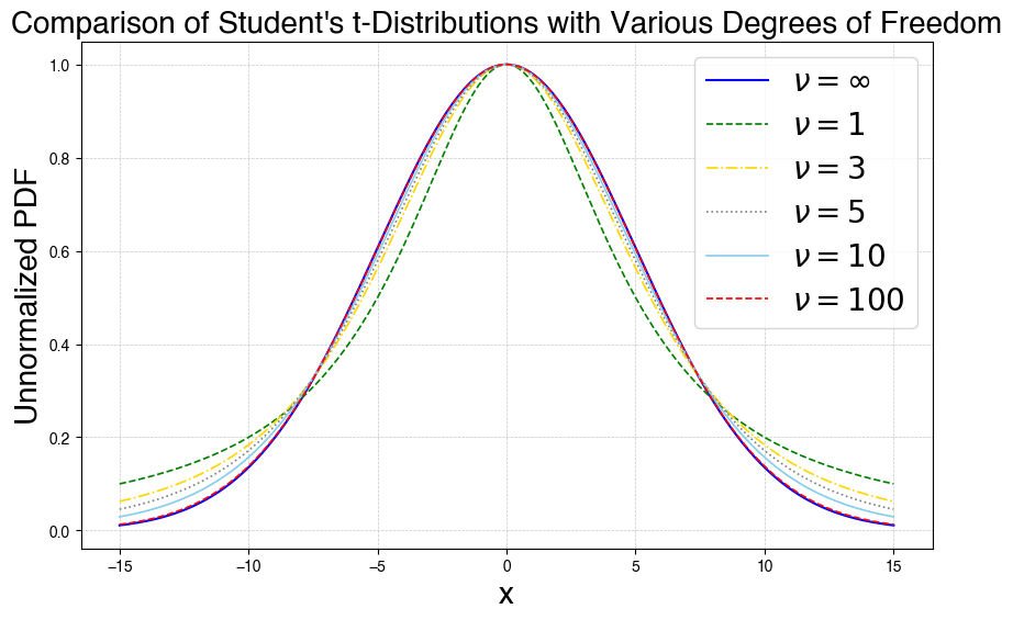
Figure 1: Student’s t with varying degrees of freedom . (standard deviation is 5).
图 1:不同自由度 下的 Student's t。(标准差为 5)。
The choice is driven by two main factors. First, t-distribution is a strong generalization of Gaussians. As shown in Fig. 1, when , ; when , . So t-distribution can capture what Gaussians capture and beyond. Furthermore, since Cauchy is fat-tailed, it can cover larger areas with higher densities than Gaussians therefore potentially reducing the number of components. As , and are learnable, SSS becomes a mixture of components learned from an infinite number of distribution families, instead of one family [14], providing further flexibility.
该选择主要由两点驱动。其一,t 分布是高斯的强推广。如图 1,当 时 ;当 时 。因此 t 分布既能覆盖高斯所能覆盖的,也能覆盖之外。此外,由于 Cauchy 重尾,它能以高于高斯的密度覆盖更大区域,从而有望减少组件数。由于 、 与 均可学习,SSS 成为从无穷多分布族中学得组件的混合,而非单一族 [14],提供进一步灵活性。
The second reason for t-distribution is it also provides good properties similar to Gaussians, e.g. close under affine transformation and marginalization of variables. Rendering a pixel requires an affine transformation, then a projective transformation, followed by an integration along a ray, to be applied to a component, which has a simple form in 3DGS. In SSS, t-distribution also has a close form:
选择 t 分布的第二理由是它也提供与高斯类似的良好性质,例如在仿射变换与变量边缘化下封闭。渲染像素需要对组件做仿射变换、再做投影变换、再沿光线积分;这在 3DGS 中有简单形式。在 SSS 中,t 分布也有闭式:
where the subscripts select the corresponding rows and columns. , and are the affine transformation (i.e. scale, translation) and (approximated) projective transformation [42, 43]. This enables us to easily derive the key gradients for learning shown in the supplementary material (SM), unlike existing research also using alternative mixture components but requiring approximation [8].
其中下标选取相应行与列。、 与 是仿射变换(即缩放、平移)与(近似)投影变换 [42, 43]。这使我们能轻松推导学习用关键梯度(见补充材料 SM),而不像同样使用替代混合组件但需要近似的现有研究 [8]。
In summary, the mixture of learnable t-distributions enhances the representational power and provides good mathematical properties for learning.
总之,可学习 t 分布混合增强了表示能力,并为学习提供良好数学性质。
3.3 Splatting and Scooping
3.3 Splatting 与 Scooping
While monotonic mixture models are powerful, a non-monotonic mixture model recently has been proposed by introducing negative components [21], arguing that it is sub-optimal to only operate in the positive density space:
单调混合模型虽强,近来有工作通过引入负组件提出非单调混合模型 [21],认为只在正密度空间操作是次优的:
where . In our problem, a negative density makes good sense as it can be seen as subtracting a color. However, our experiments using Eq. 5 show that it is not ideal as it introduces interactions between every pair of components, increasing the model evaluation complexity to where is the number of components in the model, making it significantly slower than before. Therefore, we still use Eq. 3 but with instead of where and . Normally this might cause issues as Eq. 3 is then not well defined with negative components. However, we can parameterize the density in an energy-based form explained later which is well defined. In learning, we constrain the opacity by a function so that positive and negative components can dynamically change signs while being bounded. Introducing negative t-distribution can enhance the representation power and the parameter efficiency. We show a simple experiment in Fig. 2, where fewer components are needed to fit the shape topology of a torus. In SSS, a component with negative densities is equivalent to removing its color from the mixture. Negative components are particularly useful in subtracting colors.
其中 。在我们的问题中,负密度很有意义,可视为减去一种颜色。但用式 5 的实验表明并不理想:它在每对组件间引入交互,把模型求值复杂度升到 ( 为组件数),显著变慢。因此我们仍用式 3,但令 而非 ,其中 且 。通常这可能有问题,因为带负组件时式 3 并非良定义分布;但我们可用后文基于能量的形式参数化密度,该形式良定义。学习中用不透明度经 约束,使正负组件可动态改号且有界。引入负 t 分布可增强表示力与参数效率。图 2 给出简单实验:拟合环面形状拓扑时所需组件更少。在 SSS 中,带负密度的组件等价于从混合中移除其颜色。负组件在减去颜色时尤其有用。

Figure 2: High parameter efficiency by negative components. We use a torus with only ambient lighting and frontal views (a), where the challenge is to capture the shape topology with as few components as possible. We initialize the component means near the center. Only using positive densities either underfits if two components are used (b), or requires at least 5 components to capture the topology correctly (c). In contrast, in (d), we only need two components (one positive and one negative), to capture the topology of the shape. Both components are co-located at the center of the torus. The positive component covers the torus but also the hole, while the negative component subtracts densities in the middle to make a hole.
图 2:负组件带来的高参数效率。我们使用仅有环境光与正面视角的环面 (a),挑战是用尽可能少的组件捕捉形状拓扑。组件均值初始化在中心附近。仅用正密度时,两个组件会欠拟合 (b),或至少需要 5 个组件才能正确捕捉拓扑 (c)。相较之下,在 (d) 中我们只需两个组件(一正一负)即可捕捉形状拓扑。两组件共位在环面中心:正组件覆盖环面也包括孔洞,负组件在中间减去密度以形成孔。
3.4 Learning via sampling
3.4 经由采样的学习
Recently, it is argued that principled sampling is better in 3DGS, e.g. Markov Chain Monte Carlo [15], instead of naive stochastic gradient descent (SGD). Empirically, we found training SSS involves learning more tightly coupled parameters compared with 3DGS, namely among , , and . We speculate that this is because changing in learning is changing the family of distributions within which we optimize and . Therefore, we propose a sampling scheme that mitigates such coupling, based on Stochastic Gradient Hamiltonian Monte Carlo (SGHMC).
近来有观点认为,对 3DGS 而言有原则的采样优于朴素随机梯度下降(SGD),例如马尔可夫链蒙特卡洛 [15]。经验上,我们发现训练 SSS 涉及比 3DGS 更紧密耦合的参数,尤其在 、 与 之间。我们推测,这是因为学习中改变 等于在更换我们优化 与 所在的分布族。因此我们提出基于随机梯度哈密顿蒙特卡洛(SGHMC)的采样方案以缓解这种耦合。
Starting from the Hamiltonian Monte Carlo, we first parameterize the posterior distribution as:
从哈密顿蒙特卡洛出发,我们先把后验分布参数化为:
where is our loss function, is an identity matrix, is a momentum auxiliary variable, and is the learnable parameters. This is because Eq. 3 with is not a well-defined distribution, which makes direct sampling difficult. Using an energy function circumvents this issue and prescribes the high density regions of good . Intuitively, we would like to sample to minimize . In addition, to decouple parameters during learning, the momentum term creates frictions for each dimension of the parameter space, enabling adaptive learning for each parameter.
其中 是损失函数, 是单位矩阵, 是动量辅助变量, 是可学习参数。这是因为带 的式 3 不是良定义分布,直接采样困难。用能量函数绕开该问题,并规定好 的高密度区域。直观上,我们希望采样 以最小化 。此外,动量项 在参数空间各维制造摩擦,使每个参数可自适应学习。
For , our rendering function computes the pixel value based on the components associated with a ray:
对 ,我们的渲染函数基于与光线关联的 个组件计算像素值:
where is the pixel. and are the color and opacity associated with a component . We then employ the following loss function [15]:
其中 是像素。 与 是组件 关联的颜色与不透明度。随后采用如下损失函数 [15]:
where the norm, and the structural similarity loss aim to reconstruct images, while the last two terms act as regularization, with being the eigenvalues of . The regularization applied to the opacity ensures that the opacity is big only when a component is absolutely needed. The regularization on ensures the model uses components as spiky as possible (i.e. small variances). Together, they minimize the needed number of components [15].
其中 范数与结构相似性 损失旨在重建图像,后两项起正则作用, 为 的特征值。施加于不透明度的正则保证仅在绝对需要某组件时不透明度才大;对 的正则保证模型尽量使用尖锐组件(即小方差)。二者合起来最小化所需组件数 [15]。
Furthermore, directly sampling from Eq. 6 requires the full gradient of which is not possible given the large number of training samples. Therefore, replacing the full gradient with stochastic gradient will introduce a noise term: , where is Normal and is the covariance of the stochastic gradient noise. Under mild assumptions [4], sampling Eq. 6 using stochastic gradients becomes (with detailed derivation in the SM):
此外,直接从式 6 采样需要 的全梯度,在训练样本很多时不可行。因此用随机梯度替换全梯度会引入噪声项:,其中 为正态, 为随机梯度噪声协方差。在温和假设下 [4],用随机梯度采样式 6 变为(详细推导见 SM):
where is Gaussian noise, is a mass matrix, and is a control parameter dictating the friction term and noise . In our problem, it is crucial to design good friction and noise scheduling. The effect of this principled sampling method is further discussed in SM.
其中 是高斯噪声, 是质量矩阵, 是控制参数,决定摩擦项 与噪声 。在我们的问题中,设计良好的摩擦与噪声调度至关重要。该有原则采样方法的效果在 SM 中进一步讨论。
3.4.1 Friction and Noise Scheduling
We first use SGHMC on and Adam on the other parameters. To learn , we modify Eq. 9 to:
3.4.1 摩擦与噪声调度
我们先对 用 SGHMC,对其余参数用 Adam。为学习 ,把式 9 修改为:
where is the learning rate and decays during learning. is Gaussian noise. is the opacity. The main difference between Eq. 10 and Eq. 9 is we now have adaptive friction and noise for . (sigmoid function) switches on/off the friction and noise. We use and , so that it only activates for components with opacity lower than 0.005. When it is activated, friction and noise are added to these components. Note that if is disabled, Eq. 10 is simplified to a Stochastic Gradient Langevin Dynamics scheme [33].
其中 是学习率,学习过程中衰减。 是高斯噪声。 是不透明度。式 10 与式 9 的主要差别是:我们现在对 有自适应摩擦 与噪声 。(sigmoid)开关摩擦与噪声。我们取 、,因而仅对不透明度低于 0.005 的组件激活。激活后,对这些组件加入摩擦与噪声。注意若禁用 ,式 10 简化为随机梯度朗之万动力学方案 [33]。
When learning, we initialize with a sparse set of (SfM) points without normals [14], run Eq. 10 without for burn-in for exploration, then run the full sampling for exploitation until convergence. During burn-in stage, we multiply by the covariance of the component to maintain the anisotropy profile of the t-distribution. After the burn-in, is removed, and the anisotropy is then maintained by due to the momentum .
学习时,用无无向信息的稀疏(SfM)点集初始化 [14],先不带 运行式 10 做探索性 burn-in,再运行完整采样做利用直至收敛。burn-in 阶段,把 乘以组件协方差 以保持 t 分布的各向异性轮廓。burn-in 之后去掉 ,各向异性随后由动量 驱动的 维持。
Key gradients
Overall, the key learnable parameters for each component in SSS include the mean , covariance (i.e. and ), color , opacity , and degree parameter . To compute Eq. 9, the key gradients are , ,, , , and . For simplicity, we give them in the SM.
关键梯度
总体而言,SSS 每个组件的关键可学习参数包括均值 、协方差 (即 与 )、颜色 、不透明度 与自由度参数 。为计算式 9,关键梯度是 、、、、 与 。为简洁起见,我们在 SM 中给出它们。
3.4.2 Adding and Recycling Components
Components can become nearly transparent during sampling, i.e. near zero opacity. In 3DGS, they are removed. Recently, it is argued that they should be recycled [15], by relocating them to a high opacity component. However, careful consideration needs to be taken as the overall distribution before and after relocation should be the same [27]. When moving some components to the location of another component, this is ensured by:
3.4.2 添加与回收组件
采样过程中组件可能几乎透明,即不透明度接近零。在 3DGS 中它们被移除。近来有观点认为应回收它们 [15],方法是把它们重定位到高不透明度组件处。但需仔细考虑:重定位前后整体分布应相同 [27]。当把某些组件移到另一组件位置时,由下式保证:
where and are the color after and before relocation respectively. Minimizing this integral ensures the smallest possible pixel-wise color changes over the whole domain. Minimizing Eq. 11 in SSS leads to:
其中 与 分别为重定位后与前的颜色。最小化该积分保证在整个域上像素级颜色变化尽可能小。在 SSS 中最小化式 11 得到:
$$\displaystyle\mu_{new}=\mu_{old}\text{ , }(1-o_{new})^{N}=(1-o_{old}) \ \displaystyle\Sigma_{new}=(o_{old})^{2}\frac{\nu_{old}}{\nu_{new}}(\frac{\beta(\frac{1}{2},\frac{\nu_{old}+2}{2})}{K})^{2}\Sigma_{old} \ \displaystyle K=\sum_{i=1}^{N}\sum_{k=0}^{i-1}\begin{pmatrix}i-1\
k\end{pmatrix}(-1)^{k}(o_{new})^{k+1}Z) \ \displaystyle Z=\beta(\frac{1}{2},\frac{(k+1)(\nu_{new}+3)-1}{2}) \tag{12}$$
and , and , and are the mean, opacity, and covariance after and before relocation respectively. is the total number of components after relocation, i.e. moving -1 low opacity components to the location of 1 high opacity component. is the beta function. We leave the detailed derivation in the SM. Note we do not distinguish between positive and negative components during relocation. This introduces a perturbation on the sign of the opacity. In Eq. 12, if then all , or otherwise if , regardless their original opacity signs. This sign perturbation in practice helps the mixing of the sampling. Furthermore, to ensure the sampling stability, we limit the relocation to a maximum of of the total components at a time. Finally, we also add new components when needed, but do not use the adaptive density control (clone and split) in 3DGS [14]. Instead, we add 5% new components with zero opacity and then recycle them.
与 、 与 、 与 分别为重定位后与前的均值、不透明度与协方差。 是重定位后组件总数,即把 -1 个低不透明度组件移到 1 个高不透明度组件的位置。 是 beta 函数。详细推导留在 SM。注意重定位时我们不区分正负组件。这会对不透明度符号引入扰动。在式 12 中,若 则全部 ,否则若 则 ,不论其原先符号如何。该符号扰动在实践中有助于采样混合。此外,为保证采样稳定性,我们把每次重定位限制在总组件数最多 5%。最后,需要时也会添加新组件,但不使用 3DGS 的自适应密度控制(克隆与分裂) [14]。相反,我们添加 5% 不透明度为零的新组件,再回收它们。
4 Experiments
4 实验
4.1 Experimental setting
4.1 实验设置
Datasets and Metrics
Following existing research, we employ 11 scenes from 3 datasets, including 7 public scenes from Mip-NeRF 360 [2], 2 outdoor scenes from Tanks & Temples [16], and 2 indoor scenes from Deep Blending [10]. Also, following the previous evaluation metrics, we use Peak Signal-to-Noise Ratio (PSNR), Structural Similarity Index Metric (SSIM) [32], and Learned Perceptual Image Patch Similarity (LPIPS) [41]. We provide average scores of each dataset, and detailed scores are in the SM.
数据集与指标
沿用既有研究,我们采用来自 3 个数据集的 11 个场景:Mip-NeRF 360 [2] 的 7 个公开场景、Tanks & Temples [16] 的 2 个室外场景,以及 Deep Blending [10] 的 2 个室内场景。指标同样沿用峰值信噪比(PSNR)、结构相似性指数(SSIM) [32] 与学习感知图像块相似度(LPIPS) [41]。我们给出各数据集平均分,分场景详细分数见 SM。
Baselines
Due to there being many publications based on 3DGS, we only choose the original 3DGS [14] and the most recent work that focuses on improving the fundamental paradigm of 3DGS and has achieved the best performances. The methods include Generalized Exponential Splatting (GES) [8] and 3D Half-Gaussian Splatting (3DHGS) [19] which also use different (positive only) mixture components, Scaffold-GS [22] and Fre-GS [39] which optimize the training procedure to achieve faster convergence and better results, 3DGS-MCMC [15] which proposes a principled MCMC sampling process, and Mip-NeRF [1] which is a state-of-the-art method with Neural Radiance Field (NeRF) [23]. Overall, our baselines comprehensively include methods with new mixture components, new optimization approaches, and the SOTA quality.
基线
由于基于 3DGS 的发表工作很多,我们只选择原始 3DGS [14] 以及聚焦改进 3DGS 基本范式并取得最佳表现的最新工作。方法包括同样使用不同(仅正)混合组件的 Generalized Exponential Splatting(GES) [8] 与 3D Half-Gaussian Splatting(3DHGS) [19],优化训练过程以更快收敛、更好结果的 Scaffold-GS [22] 与 Fre-GS [39],提出有原则 MCMC 采样的 3DGS-MCMC [15],以及神经辐射场(NeRF) [23] 的 SOTA 方法 Mip-NeRF [1]。总体而言,基线全面覆盖新混合组件、新优化方法与 SOTA 质量三类。
The results of all baselines in general benchmarking are from their papers. In addition, we run their codes with other settings for more comparison. Since not all baseline methods are implemented in exactly the same setting, we need to adapt them for comparison. These details are in the SM.
一般基准中全部基线结果来自其论文。此外我们在其他设定下运行其代码以做更多对比。由于并非所有基线都在完全相同设定下实现,我们需要适配它们以便对比。细节见 SM。
4.2 General Benchmarks
4.2 一般基准
| Dataset | Mip-NeRF360 Dataset | Tanks&Temples | Deep Blending | ||||||
|---|---|---|---|---|---|---|---|---|---|
| Method—Metric | PSNR | SSIM | LPIPS | PSNR | SSIM | LPIPS | PSNR | SSIM | LPIPS |
| Mip-NeRF | 29.23 | 0.844 | 0.207 | 22.22 | 0.759 | 0.257 | 29.40 | 0.901 | 0.245 |
| 3DGS | 28.69 | 0.870 | 0.182 | 23.14 | 0.841 | 0.183 | 29.41 | 0.903 | 0.243 |
| GES | 26.91 | 0.794 | 0.250 | 23.35 | 0.836 | 0.198 | 29.68 | 0.901 | 0.252 |
| 3DHGS | 29.56 | 0.873 | 0.178 | 24.49 | 0.857 | 0.169 | 29.76 | 0.905 | 0.242 |
| Fre-GS | 27.85 | 0.826 | 0.209 | 23.96 | 0.841 | 0.183 | 29.93 | 0.904 | 0.240 |
| Scaffold-GS | 28.84 | 0.848 | 0.220 | 23.96 | 0.853 | 0.177 | 30.21 | 0.906 | 0.254 |
| 3DGS-MCMC | 29.89 | 0.900 | 0.190 | 24.29 | 0.860 | 0.190 | 29.67 | 0.890 | 0.320 |
| Ours | 29.90 | 0.893 | 0.145 | 24.87 | 0.873 | 0.138 | 30.07 | 0.907 | 0.247 |
Table 1: Comparison. The red, orange and yellow colors represent the top three results. Competing metrics are extracted from respective papers, and ours are reported as the average of three runs.
| 数据集 | Mip-NeRF360 Dataset | Tanks&Temples | Deep Blending | ||||||
|---|---|---|---|---|---|---|---|---|---|
| 方法—指标 | PSNR | SSIM | LPIPS | PSNR | SSIM | LPIPS | PSNR | SSIM | LPIPS |
| Mip-NeRF | 29.23 | 0.844 | 0.207 | 22.22 | 0.759 | 0.257 | 29.40 | 0.901 | 0.245 |
| 3DGS | 28.69 | 0.870 | 0.182 | 23.14 | 0.841 | 0.183 | 29.41 | 0.903 | 0.243 |
| GES | 26.91 | 0.794 | 0.250 | 23.35 | 0.836 | 0.198 | 29.68 | 0.901 | 0.252 |
| 3DHGS | 29.56 | 0.873 | 0.178 | 24.49 | 0.857 | 0.169 | 29.76 | 0.905 | 0.242 |
| Fre-GS | 27.85 | 0.826 | 0.209 | 23.96 | 0.841 | 0.183 | 29.93 | 0.904 | 0.240 |
| Scaffold-GS | 28.84 | 0.848 | 0.220 | 23.96 | 0.853 | 0.177 | 30.21 | 0.906 | 0.254 |
| 3DGS-MCMC | 29.89 | 0.900 | 0.190 | 24.29 | 0.860 | 0.190 | 29.67 | 0.890 | 0.320 |
| Ours | 29.90 | 0.893 | 0.145 | 24.87 | 0.873 | 0.138 | 30.07 | 0.907 | 0.247 |
表 1:对比。 红、橙、黄分别表示前三名结果。对照指标摘自各自论文,我们的结果为三次运行平均。
We first compare SSS with the baselines on all scenes in their default settings, shown in Tab. 1. SSS achieves overall the best results on 6 of the 9 metrics, and the second best on 2 metrics. The only exception is the LPIPS in Deep Blending, where the difference between SSS and the best is 710*-3*. Furthermore, when investigating individual scenes, SSS achieves the largest leading margin on Train. It achieves 23.23/0.844/0.170, where the second best method 3DHGS achieves 22.95/0.827/0.197, in PSNR, SSIM, and LPIPS, which is a 1.22%/2.05%/13.7% improvement. Detailed scores for each scene are in the SM. We show qualitative comparison in Figure 3.
我们先在默认设定下于全部场景比较 SSS 与基线,见表 1。SSS 在 9 项指标中的 6 项总体最佳,2 项第二。唯一例外是 Deep Blending 的 LPIPS,SSS 与最佳相差 。进一步看各场景,SSS 在 Train 上领先幅度最大:达到 23.23/0.844/0.170,而次优 3DHGS 为 22.95/0.827/0.197(PSNR/SSIM/LPIPS),分别提升 1.22%/2.05%/13.7%。各场景详细分数见 SM。定性对比见图 3。
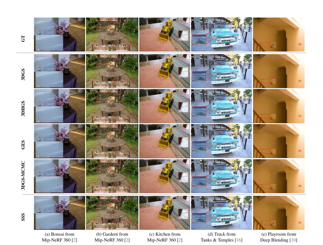
Figure 3: Visual comparison Zoom-in for better visualization. (a) SSS restores better the indentations of the box lid; (b) SSS is the best at detailing windows in the upper center; (c) Only the image rendered by SSS contains the green track detail in the upper right corner; (d) SSS is the best at restoring the reflection in the front window of the truck; (e) SSS perfectly restores the light switch next to the stairs.
图 3:视觉对比,建议放大查看。(a) SSS 更好恢复盒盖凹痕;(b) SSS 在上部中央窗细节上最佳;(c) 仅 SSS 渲染图像右上角含绿色轨道细节;(d) SSS 最佳恢复卡车前窗反射;(e) SSS 完美恢复楼梯旁电灯开关。
4.3 Parameter Efficiency
4.3 参数效率
SSS has stronger representation power than 3DGS and its variants. The varying tail-thickness of its components enables SSS to fit the data with fewer components, i.e. higher parameter efficiency. We show this via experiments under different component numbers.
SSS 比 3DGS 及其变体有更强表示能力。组件尾部厚度可变,使 SSS 能用更少组件拟合数据,即更高参数效率。我们通过不同组件数下的实验展示这一点。
Since the SfM initialization gives different components in different scenes and a method normally increases the component number during learning, we introduce a coefficient to describe the latter as a multiplicity of the former. Denoting the initial component number as , we test , 1.4, 1.8, 2.2, and 2.6 as the maximum component number for comparison. Note even with 2.6, the component number is still much smaller than the experiments in Tab. 1. Specifically, the 2.6 vs the original 3DGS component number are 468k/1.1m, 364k/2.6m, 208k/3.4m, 96k/2.5m, 140k/5.9m, 520k/1.3m, 416k/1.2m, 364k/5.2m, 624k/1.8m, 286k/1.5m, 83k/4.75m, in Train, Truck, DrJohnson, Playroom, Bicycle, Bonsai, Counter, Garden, Kitchen, Room, Stump, corresponding to merely 42.5%, 14%, 6.1%, 3.8%, 2.4%, 40%, 34.7%, 7%, 34.7%, 19.1%, 1.7% of the original components, a maximum of 98.3% reduction.
由于 SfM 初始化在不同场景给出不同组件数,且方法通常在学习中增加组件数,我们引入系数把后者描述为前者的倍数。记初始组件数为 ,测试 、1.4、1.8、2.2 与 2.6 作为对比的最大组件数。注意即便用 2.6,组件数仍远小于表 1 实验。具体地,2.6 相对原始 3DGS 组件数在 Train、Truck、DrJohnson、Playroom、Bicycle、Bonsai、Counter、Garden、Kitchen、Room、Stump 上分别为 468k/1.1m、364k/2.6m、208k/3.4m、96k/2.5m、140k/5.9m、520k/1.3m、416k/1.2m、364k/5.2m、624k/1.8m、286k/1.5m、83k/4.75m,仅相当于原始组件的 42.5%、14%、6.1%、3.8%、2.4%、40%、34.7%、7%、34.7%、19.1%、1.7%,最多减少 98.3%。
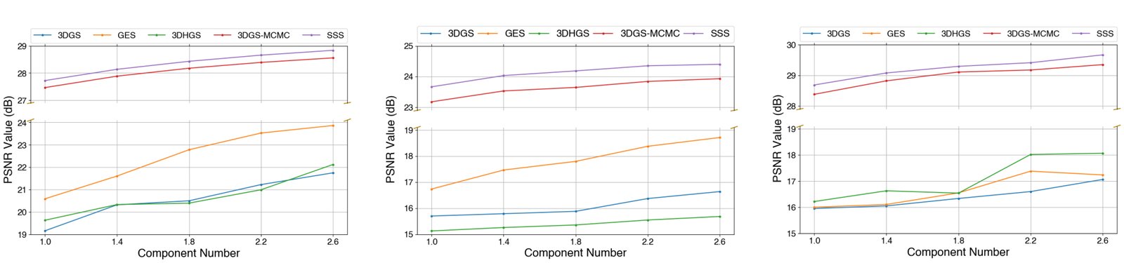
Figure 4: All methods with reduced component numbers.
图 4:各方法在减少组件数设定下的结果。
PSNR is averaged over the scenes in each dataset and shown in Figure 4. First, SSS outperforms all other methods in 15 out of 15 settings, demonstrating strong expressivity across all scenarios. Furthermore, when the component number decreases, all methods deteriorate, but SSS deteriorates slowly comparatively, demonstrating that SSS can fit the data much more efficiently than the rest. One specific example is the Tanks & Temples in Tab. 1. SSS achieves 23.6 PSNR with merely 180k components, already surpassing Mip-NeFR, 3DGS and GES. With around 300k components, SSS achieves 24.4 PSNR, which is only slightly worse than 3DHGS and 3DGS-MCMC, by a margin at the scale of 10*-2*. Note this is a comparison with the methods in Tab. 1 where they use at least 1m components, e.g. 3DGS employs around 1.1m and 2.6m in Train and Truck, while SSS employs only around 364k and 468k, a maximum reduction of 82% of the components.
PSNR 在各数据集场景上平均,见图 4。首先,SSS 在全部 15/15 设定中优于其他方法,展示跨场景的强表达力。此外,组件数减少时所有方法都变差,但 SSS 相对变差更慢,说明 SSS 拟合数据远比其余方法高效。一个具体例子是表 1 中的 Tanks & Temples:SSS 仅用约 180k 组件就达到 23.6 PSNR,已超过 Mip-NeRF、3DGS 与 GES;约 300k 组件时达 24.4 PSNR,仅略逊于 3DHGS 与 3DGS-MCMC,差距在 量级。注意这是与表 1 中至少使用约 1m 组件的方法对比,例如 3DGS 在 Train 与 Truck 约用 1.1m 与 2.6m,而 SSS 仅约 364k 与 468k,组件最多减少约 82%。
4.4 Qualitative Comparison
4.4 定性对比
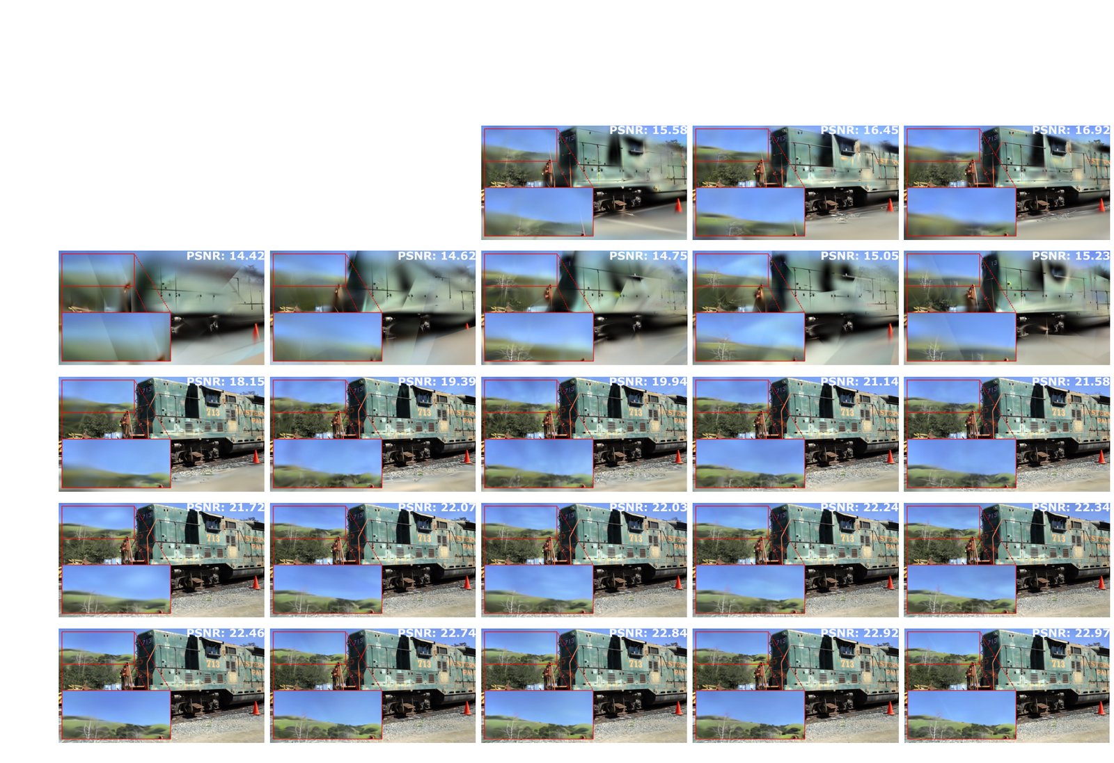
Figure 5: Visual results of all methods with varying component numbers. In addition to the well-reconstructed main body of the train compared to other baselines, our method can use a small number of components to restore more details, such as plants on distant mountains, rocks on the ground nearby, etc. Besides, our sky has fewer noises and appears more similarly to the ground truth. Zoom in for details. Note that ours with 252k components has already achieved SOTA quality and beats most baselines.
图 5:各方法在不同组件数下的视觉结果。除相对其他基线更好重建火车主体外,我们的方法能用少量组件恢复更多细节,如远山植物、近处地面岩石等。此外我们的天空噪声更少,更接近真值。建议放大查看细节。注意我们用 252k 组件已达 SOTA 质量并超过多数基线。
We further show a qualitative comparison in one scene across the different component numbers in Fig. 5. The ground-truth is one view from the Train. When restricting the component number to around 180k, the original 3DGS and one of the state-of-the-art methods 3DHGS show significant blur. This is likely to be caused by the struggle between stretching Gaussians to cover large areas and narrowing them to reconstruct details, given a limited number of components at proposal. Due to the optimization relying on stochastic gradient descent, a local minimum is sought where the distribution of the Gaussians is sub-optimal. Intuitively, the issue can be mitigated by more flexible components and/or better optimization. As expected, this is shown in GES and 3DGS-MCMC, where the former employs a more flexible component (generalized exponential function) while the latter improves the optimization itself by MCMC. The improvements by both methods suggest that these are the correct directions to improve the paradigm of 3DGS.
我们进一步在图 5 中展示同一场景跨不同组件数的定性对比。真值是 Train 的一个视角。当把组件数限制在约 180k 时,原始 3DGS 与 SOTA 之一 3DHGS 出现明显模糊。这很可能来自在组件数有限时,在「拉长高斯覆盖大区域」与「收窄高斯重建细节」之间的挣扎。由于优化依赖随机梯度下降,会寻到高斯分布次优的局部极小。直观上,更灵活组件和/或更好优化可缓解该问题。果然,GES 与 3DGS-MCMC 体现了这一点:前者用更灵活组件(广义指数函数),后者用 MCMC 改进优化本身。二者的改进表明这些是改进 3DGS 范式的正确方向。
Next, SSS outperforms GES and 3DGS-MCMC visually when using 180k components. One example is the sky and the hill in the background in the left half of the image. GES creates a blurry background mixing the sky and the hill, with no discernible details, suggesting it uses a few components that are stretched to cover large areas. In contrast, 3DGS-MCMC can separate the sky from the hill. But it creates random white patches in the sky, which do not exist in the ground truth. This suggests that 3DGS-MCMC employs a relatively larger number of slim Gaussians to fit the details but meanwhile introduces additional noises. SSS not only successfully separates the sky and the hill, but simultaneously retains the homogeneous color in the sky and reconstructs the details on the hill, e.g. the trees and lawns. This is attributed to SSS’ capability of learning components with varying tail-fatness to adaptively capture large homogeneous areas and small heterogeneous regions.
接着,在使用 180k 组件时,SSS 在视觉上优于 GES 与 3DGS-MCMC。一例是图像左半背景的天空与山丘。GES 产生把天空与山丘混在一起的模糊背景,无明显细节,说明它用少数被拉长的组件覆盖大区域。相较之下,3DGS-MCMC 能分开天空与山丘,但在天空制造真值中不存在的随机白斑,说明它用相对更多细长高斯拟合细节,同时引入额外噪声。SSS 不仅成功分开天空与山丘,还同时保持天空均匀颜色并重建山丘细节(如树木与草坪)。这归因于 SSS 能学习尾部胖瘦可变的组件,自适应捕捉大片均匀区域与小片异质区域。
Furthermore, when increasing the component number to 468k, all results are improved, as expected. 3DGS and 3DHGS still cannot work as well as other methods, suggesting they need more components. In addition, the difference between GES, 3DGS-MCMC, and SSS starts to narrow. GES can separate the sky and the hill. Both GES and 3DGS-MCMC have fewer artifacts. However, as the component number increases, there are still noticeable noises introduced to the sky, which suggests that it is a common issue for both methods when using more components to cover an area with mixed homogeneous and heterogeneous regions. Comparatively, SSS gives consistent performance across all component numbers, i.e. clearly separating and reconstructing the homogeneous sky and the heterogeneous hill. Also, the visual quality from 180k to 468k does not change significantly for SSS, but is noticeably improved for GES and 3DGS-MCMC, suggesting a higher parameter efficiency of SSS in perception.
进一步把组件数增至 468k 时,所有结果都如预期改进。3DGS 与 3DHGS 仍不及其他方法,说明它们需要更多组件。此外 GES、3DGS-MCMC 与 SSS 之间差距开始缩小。GES 能分开天空与山丘;GES 与 3DGS-MCMC 伪影都更少。但随着组件数增加,天空仍有明显噪声,说明两方法在用更多组件覆盖均匀与异质混合区域时有共性问题。相较之下,SSS 在全部组件数上表现一致,即清晰分开并重建均匀天空与异质山丘。并且从 180k 到 468k,SSS 视觉质量变化不大,而 GES 与 3DGS-MCMC 有明显改进,说明 SSS 在感知上参数效率更高。
Ablation Study
We conduct an ablation study to show the effectiveness of various components in SSS. These results prove how each component contributes to the final performance improvement. We give details in the SM.
消融研究
我们做消融以展示 SSS 各组件有效性。这些结果证明每个组件如何贡献最终性能提升。细节见 SM。
5 Conclusion, Discussion, and Future Work
5 结论、讨论与未来工作
We proposed Student Splatting and Scooping (SSS), a new non-monotonic mixture model, consisting of positive and negative Student’s t distributions, learned by a principled SGHMC sampling. SSS contains a simple yet strong and non-trivial generalization of 3DGS and its variants. SSS outperforms existing methods in rendering quality, and shows high parameter efficiency, e.g. achieving comparable quality with less than of components.
我们提出 Student Splatting and Scooping(SSS):由正负 Student's t 分布构成、经有原则 SGHMC 采样学习的新非单调混合模型。SSS 包含对 3DGS 及其变体简单却强且非平凡的推广。SSS 在渲染质量上优于现有方法,并展示高参数效率,例如用不到 的组件达到可比质量。
SSS has limitations. Its primitives are restricted to symmetric and smooth t-distributions, limiting its representation. The sampling also needs hyperparameter tuning such as the percentage of negative components. In the future, we will combine other distribution families (e.g. Laplace) with t-distribution to further enhance the expressivity, and make the SGHMC self-adaptive to achieve better balances between the positive and negative components.
SSS 也有局限。其图元限于对称光滑的 t 分布,限制表示能力。采样也需超参调优,例如负组件比例。未来我们将把其他分布族(如 Laplace)与 t 分布结合以进一步增强表达力,并使 SGHMC 自适应,以在正负组件之间取得更好平衡。
Acknowledgement
致谢
This project has received funding from the European Union’s Horizon 2020 research and innovation programme under grant agreement No 899739 CrowdDNA.
本项目获欧盟地平线 2020 研究与创新计划资助,协议编号 899739 CrowdDNA。
References
参考文献
3D Student Splatting and Scooping
Supplementary Material
补充材料
Jialin Zhu1, Jiangbei Yue2, Feixiang He1, He Wang1,3
1University College London, UK 2University of Leeds, UK
3AI Centre, University College London, UK
[1] Jonathan T Barron, Ben Mildenhall, Matthew Tancik, Peter Hedman, Ricardo Martin-Brualla, and Pratul P Srinivasan. Mip-nerf: A multiscale representation for anti-aliasing neural radiance fields. In Proceedings of the IEEE/CVF international conference on computer vision , pages 5855–5864, 2021.
[2] Jonathan T Barron, Ben Mildenhall, Dor Verbin, Pratul P Srinivasan, and Peter Hedman. Mip-nerf 360: Unbounded anti-aliased neural radiance fields. In Proceedings of the IEEE/CVF conference on computer vision and pattern recognition , pages 5470–5479, 2022.
[3] Guikun Chen and Wenguan Wang. A survey on 3d gaussian splatting. arXiv preprint arXiv:2401.03890 , 2024.
[4] Tianqi Chen, Emily Fox, and Carlos Guestrin. Stochastic gradient hamiltonian monte carlo. In International conference on machine learning , pages 1683–1691. PMLR, 2014.
[5] Zhiqin Chen, Thomas Funkhouser, Peter Hedman, and Andrea Tagliasacchi. Mobilenerf: Exploiting the polygon rasterization pipeline for efficient neural field rendering on mobile architectures. In Proceedings of the IEEE/CVF Conference on Computer Vision and Pattern Recognition , pages 16569–16578, 2023.
[6] Ben Fei, Jingyi Xu, Rui Zhang, Qingyuan Zhou, Weidong Yang, and Ying He. 3d gaussian as a new vision era: A survey. arXiv preprint arXiv:2402.07181 , 2024.
[7] Sara Fridovich-Keil, Alex Yu, Matthew Tancik, Qinhong Chen, Benjamin Recht, and Angjoo Kanazawa. Plenoxels: Radiance fields without neural networks. In Proceedings of the IEEE/CVF conference on computer vision and pattern recognition , pages 5501–5510, 2022.
[8] Abdullah Hamdi, Luke Melas-Kyriazi, Jinjie Mai, Guocheng Qian, Ruoshi Liu, Carl Vondrick, Bernard Ghanem, and Andrea Vedaldi. Ges: Generalized exponential splatting for efficient radiance field rendering. In Proceedings of the IEEE/CVF Conference on Computer Vision and Pattern Recognition , pages 19812–19822, 2024.
[9] N Alan Heckert, James J Filliben, C M Croarkin, B Hembree, William F Guthrie, P Tobias, and J Prinz. Handbook 151: Nist/sematech e-handbook of statistical methods. 2002.
[10] Peter Hedman, Julien Philip, True Price, Jan-Michael Frahm, George Drettakis, and Gabriel Brostow. Deep blending for free-viewpoint image-based rendering. ACM Transactions on Graphics (ToG) , 37(6):1–15, 2018.
[11] Peter Hedman, Pratul P Srinivasan, Ben Mildenhall, Jonathan T Barron, and Paul Debevec. Baking neural radiance fields for real-time view synthesis. In Proceedings of the IEEE/CVF international conference on computer vision , pages 5875–5884, 2021.
[12] Binbin Huang, Zehao Yu, Anpei Chen, Andreas Geiger, and Shenghua Gao. 2d gaussian splatting for geometrically accurate radiance fields. In ACM SIGGRAPH 2024 Conference Papers , pages 1–11, 2024a.
[13] Letian Huang, Jiayang Bai, Jie Guo, and Yanwen Guo. Gs++: Error analyzing and optimal gaussian splatting. arXiv preprint arXiv:2402.00752 , 2024b.
[14] Bernhard Kerbl, Georgios Kopanas, Thomas Leimkühler, and George Drettakis. 3d gaussian splatting for real-time radiance field rendering. ACM Trans. Graph. , 42(4):139–1, 2023.
[15] Shakiba Kheradmand, Daniel Rebain, Gopal Sharma, Weiwei Sun, Yang-Che Tseng, Hossam Isack, Abhishek Kar, Andrea Tagliasacchi, and Kwang Moo Yi. 3d gaussian splatting as markov chain monte carlo. Advances in Neural Information Processing Systems , 37:80965–80986, 2024.
[16] Arno Knapitsch, Jaesik Park, Qian-Yi Zhou, and Vladlen Koltun. Tanks and temples: Benchmarking large-scale scene reconstruction. ACM Transactions on Graphics (ToG) , 36(4):1–13, 2017.
[17] Jonas Kulhanek, Songyou Peng, Zuzana Kukelova, Marc Pollefeys, and Torsten Sattler. WildGaussians: 3D gaussian splatting in the wild. NeurIPS , 2024.
[18] Joo Chan Lee, Daniel Rho, Xiangyu Sun, Jong Hwan Ko, and Eunbyung Park. Compact 3d gaussian representation for radiance field. In Proceedings of the IEEE/CVF Conference on Computer Vision and Pattern Recognition , pages 21719–21728, 2024.
[19] Haolin Li, Jinyang Liu, Mario Sznaier, and Octavia Camps. 3d-hgs: 3d half-gaussian splatting. arXiv preprint arXiv:2406.02720 , 2024.
[20] Ruoshi Liu, Rundi Wu, Basile Van Hoorick, Pavel Tokmakov, Sergey Zakharov, and Carl Vondrick. Zero-1-to-3: Zero-shot one image to 3d object. In Proceedings of the IEEE/CVF international conference on computer vision , pages 9298–9309, 2023.
[21] Lorenzo Loconte, Aleksanteri Sladek, Stefan Mengel, Martin Trapp, Arno Solin, Nicolas Gillis, and Antonio Vergari. Subtractive mixture models via squaring: Representation and learning. In International Conference on Learning Representations (ICLR) , 2024.
[22] Tao Lu, Mulin Yu, Linning Xu, Yuanbo Xiangli, Limin Wang, Dahua Lin, and Bo Dai. Scaffold-gs: Structured 3d gaussians for view-adaptive rendering. In Proceedings of the IEEE/CVF Conference on Computer Vision and Pattern Recognition , pages 20654–20664, 2024.
[23] Ben Mildenhall, Pratul P Srinivasan, Matthew Tancik, Jonathan T Barron, Ravi Ramamoorthi, and Ren Ng. Nerf: Representing scenes as neural radiance fields for view synthesis. Communications of the ACM , 65(1):99–106, 2021.
[24] Thomas Müller, Alex Evans, Christoph Schied, and Alexander Keller. Instant neural graphics primitives with a multiresolution hash encoding. ACM transactions on graphics (TOG) , 41(4):1–15, 2022.
[25] Ben Poole, Ajay Jain, Jonathan T Barron, and Ben Mildenhall. Dreamfusion: Text-to-3d using 2d diffusion. In The Eleventh International Conference on Learning Representations .
[26] Albert Pumarola, Enric Corona, Gerard Pons-Moll, and Francesc Moreno-Noguer. D-nerf: Neural radiance fields for dynamic scenes. In Proceedings of the IEEE/CVF Conference on Computer Vision and Pattern Recognition , pages 10318–10327, 2021.
[27] Samuel Rota Bulò, Lorenzo Porzi, and Peter Kontschieder. Revising densification in gaussian splatting. In European Conference on Computer Vision , pages 347–362. Springer, 2024.
[28] Steven M Seitz, Brian Curless, James Diebel, Daniel Scharstein, and Richard Szeliski. A comparison and evaluation of multi-view stereo reconstruction algorithms. In 2006 IEEE computer society conference on computer vision and pattern recognition (CVPR’06) , pages 519–528. IEEE, 2006.
[29] Xiangyu Sun, Joo Chan Lee, Daniel Rho, Jong Hwan Ko, Usman Ali, and Eunbyung Park. F-3dgs: Factorized coordinates and representations for 3d gaussian splatting. In Proceedings of the 32nd ACM International Conference on Multimedia , pages 7957–7965, 2024.
[30] Jiaxiang Tang, Jiawei Ren, Hang Zhou, Ziwei Liu, and Gang Zeng. Dreamgaussian: Generative gaussian splatting for efficient 3d content creation. In The Twelfth International Conference on Learning Representations .
[31] Shimon Ullman. The interpretation of structure from motion. Proceedings of the Royal Society of London. Series B. Biological Sciences , 203(1153):405–426, 1979.
[32] Zhou Wang, Alan C Bovik, Hamid R Sheikh, and Eero P Simoncelli. Image quality assessment: from error visibility to structural similarity. IEEE transactions on image processing , 13(4):600–612, 2004.
[33] Max Welling and Yee W Teh. Bayesian learning via stochastic gradient langevin dynamics. In Proceedings of the 28th international conference on machine learning (ICML-11) , pages 681–688. Citeseer, 2011.
[34] Guanjun Wu, Taoran Yi, Jiemin Fang, Lingxi Xie, Xiaopeng Zhang, Wei Wei, Wenyu Liu, Qi Tian, and Xinggang Wang. 4d gaussian splatting for real-time dynamic scene rendering. In Proceedings of the IEEE/CVF Conference on Computer Vision and Pattern Recognition , pages 20310–20320, 2024.
[35] Minye Wu and Tinne Tuytelaars. Implicit gaussian splatting with efficient multi-level tri-plane representation. arXiv preprint arXiv:2408.10041 , 2024.
[36] Ziyi Yang, Xinyu Gao, Wen Zhou, Shaohui Jiao, Yuqing Zhang, and Xiaogang Jin. Deformable 3d gaussians for high-fidelity monocular dynamic scene reconstruction. In Proceedings of the IEEE/CVF Conference on Computer Vision and Pattern Recognition , pages 20331–20341, 2024.
[37] Vickie Ye and Angjoo Kanazawa. Mathematical supplement for the gsplat library. arXiv preprint arXiv:2312.02121 , 2023.
[38] Zehao Yu, Anpei Chen, Binbin Huang, Torsten Sattler, and Andreas Geiger. Mip-splatting: Alias-free 3d gaussian splatting. In Proceedings of the IEEE/CVF Conference on Computer Vision and Pattern Recognition , pages 19447–19456, 2024.
[39] Jiahui Zhang, Fangneng Zhan, Muyu Xu, Shijian Lu, and Eric Xing. Fregs: 3d gaussian splatting with progressive frequency regularization. In Proceedings of the IEEE/CVF Conference on Computer Vision and Pattern Recognition , pages 21424–21433, 2024.
[40] Kai Zhang, Gernot Riegler, Noah Snavely, and Vladlen Koltun. Nerf++: Analyzing and improving neural radiance fields. arXiv preprint arXiv:2010.07492 , 2020.
[41] Richard Zhang, Phillip Isola, Alexei A Efros, Eli Shechtman, and Oliver Wang. The unreasonable effectiveness of deep features as a perceptual metric. In Proceedings of the IEEE conference on computer vision and pattern recognition , pages 586–595, 2018.
[42] Matthias Zwicker, Hanspeter Pfister, Jeroen Van Baar, and Markus Gross. Ewa volume splatting. In Proceedings Visualization, 2001. VIS’01. , pages 29–538. IEEE, 2001.
[43] Matthias Zwicker, Hanspeter Pfister, Jeroen Van Baar, and Markus Gross. Ewa splatting. IEEE Transactions on Visualization and Computer Graphics , 8(3):223–238, 2002.
1 Additional Experimental Results
1 额外实验结果
We show more visual results of general benchmarks for Student Splatting and Scooping (SSS) against selected baselines: 3D Gaussian Splatting (3DGS) [14], 3D Half-Gaussian Splatting (3DHGS) [19], Generalized Exponential Splattin (GES) [8] and 3D Gaussian Splatting as Markov Chain Monte Carlo (3DGS-MCMC) [15] in Fig. 1. For (a) in Fig. 1, there are a few food residues in the metal bowl. Only 3DGS-MCMC and SSS can successfully restore these details. Furthermore, SSS also achieves a better reconstruction of colors than 3DGS-MCMC with these residues. SSS is the only method that can reproduce the sharp details of the chair refracted in the transparent water glass in Fig. 1 (b). For (c) in Fig. 1, the difficulty lies in reconstructing the details of the upper wall edge and the items on the cabinet (texts, etc.). Considering these two difficulties, SSS performs best in this scenario. SSS can also ensure that the details at the edge of the image are restored to the greatest extent, which is reflected in (d) and (e) of Fig. 1. In addition, SSS is also the best for reconstructing pure color areas (sky, wall, etc.).
我们展示 Student Splatting and Scooping(SSS)相对选定基线——3D Gaussian Splatting(3DGS) [14]、3D Half-Gaussian Splatting(3DHGS) [19]、Generalized Exponential Splatting(GES) [8] 与 3D Gaussian Splatting as Markov Chain Monte Carlo(3DGS-MCMC) [15]——在一般基准上的更多视觉结果,见图 1。对图 1 (a),金属碗内有少量食物残渣;仅 3DGS-MCMC 与 SSS 能成功恢复这些细节,且 SSS 对这些残渣的颜色重建优于 3DGS-MCMC。图 1 (b) 中,SSS 是唯一能重现透明水杯折射出的椅子尖锐细节的方法。图 1 (c) 的难点在于重建上墙边缘细节与柜上物品(文字等);综合这两点,SSS 在该场景表现最佳。SSS 也能最大程度恢复图像边缘细节,见图 1 (d)(e)。此外,对纯色区域(天空、墙面等)SSS 也最佳。
We have illustrated the results of the Train scene in the Tanks & Temples dataset [16] in the main context for the varying component numbers experiment. Here we further show two more scenes (room from Mip-MeRF 360 [2] and drjohnson from Deep Blending [10]) in Figs. 2 and 3. In Fig. 2, the difficulty of 3D reconstruction lies in the texture of the carpet. Both 3DGS, 3DHGS, and GES can only restore the approximate shape but cannot take into account the details when the number of components is small. 3DGS-MCMC and SSS can restore the details of the carpet. However, because SSS has a scooping operation, the carpet it reconstructs has a more realistic texture. 3DGS, 3DHGS, and GES are completely unable to reconstruct quality results in the setting of 80k to 208k components in Fig. 3. The reconstruction of 3DGS-MCMC is good enough but loses some details (window gaps inside the basket marked area), while SSS is still the best method for capturing details.
我们已在正文中展示 Tanks & Temples 数据集 [16] Train 场景上变化组件数实验的结果。这里再展示两个场景(Mip-NeRF 360 [2] 的 room 与 Deep Blending [10] 的 drjohnson),见图 2 与图 3。图 2 中三维重建难点在地毯纹理:组件数较少时,3DGS、3DHGS 与 GES 只能恢复大致形状而顾不上细节;3DGS-MCMC 与 SSS 能恢复地毯细节,但因 SSS 有 scooping 操作,其重建地毯纹理更真实。图 3 中在 80k–208k 组件设定下,3DGS、3DHGS 与 GES 完全无法重建出合格结果;3DGS-MCMC 重建已够好但丢失部分细节(篮框标记区内窗缝),而 SSS 仍是捕捉细节的最佳方法。
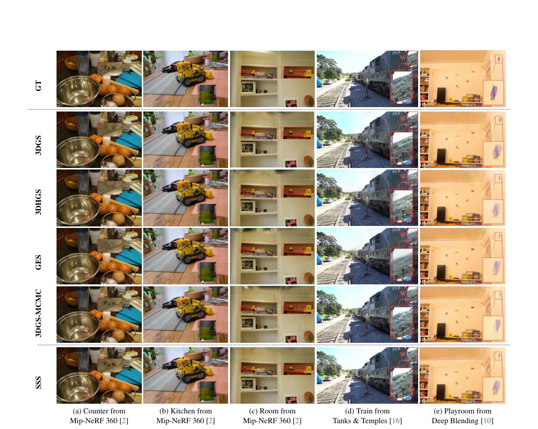
Figure 1: Visual comparison. (a) SSS restores the best details inside the metal bowl. (b) SSS is the only one that can reconstruct the details of the chair refracted in the transparent cup. (c) The reconstruction of the wall edge (bright blue box) and the font were both done best by SSS. (d) SSS’s details on the distant woods and the reconstruction of the sky are the best. (e) The reconstruction of the pattern on the wall is SSS at its best.
图 1:视觉对比。(a) SSS 最佳恢复金属碗内细节。(b) SSS 是唯一能重建透明杯中折射椅子细节的方法。(c) 墙缘(亮蓝框)与字体重建均由 SSS 做得最好。(d) SSS 对远方树林细节与天空重建最佳。(e) 墙面图案重建以 SSS 最佳。
1.1 Detailed Results on Each Scene
1.1 各场景详细结果
We show detailed comparisons between our method and the baselines on every scene on Peak Signal-to-Noise Ratio (PSNR), Structural Similarity Index Metric (SSIM) [32], and Learned Perceptual Image Patch Similarity (LPIPS) [41] metrics among three datasets (Mip-NeRF 360 [2], Tanks & Temples [16], Deep Blending [10]) in Tabs. 1, 2, 3, 4, 5 and 6.
我们在三个数据集(Mip-NeRF 360 [2]、Tanks & Temples [16]、Deep Blending [10])的每个场景上,用峰值信噪比(PSNR)、结构相似性指数(SSIM) [32] 与学习感知图像块相似度(LPIPS) [41],展示本方法与基线的详细对比,见表 1–6。
Note we only include baselines that provide detailed evaluation scores on each scene. These baselines are Mip-NeRF [1], 3DGS [14], Scaffold-GS [22], 3DHGS [19] and 3DGS-MCMC [15]. This is due to the intrinsic randomness in the training of these methods. When we re-train the models ourselves and often obtain slightly different results from their papers. Therefore, we use the results reported in their original papers.
注意我们只纳入提供各场景详细评测分数的基线:Mip-NeRF [1]、3DGS [14]、Scaffold-GS [22]、3DHGS [19] 与 3DGS-MCMC [15]。这是因为这些方法训练存在固有随机性;我们自行重训时常得到与其论文略有不同的结果。因此我们使用其原文报告的结果。
Overall, our method outperforms all the baselines. A close second is 3DGS-MCMC, which is a state-of-the-art model recently. There are some baselines that outperform both our method and 3DGS-MCMC on individual scenes under some metrics, but overall, our method and 3DGS-MCMC are the best and second best methods.
总体而言,本方法优于全部基线。紧随其后的是近期 SOTA 模型 3DGS-MCMC。在个别场景与个别指标上,有些基线会超过本方法与 3DGS-MCMC,但总体本方法与 3DGS-MCMC 分列第一、第二。
Beyond the selected methods for baseline, we do realize that there might be other methods that are not included here but achieve higher scores on certain scenes and metrics, especially when it comes to specific application settings, e.g. 3D reconstruction. However, our goal here is to restrict our comparison to the methods that aim to improve 3DGS on its fundamental formulation and can be potentially used as a generic-purposed component.
在选定基线之外,我们意识到可能还有未纳入、但在某些场景与指标上得分更高的方法,尤其在特定应用设定下,例如三维重建。但我们的目标是把对比限制在旨在改进 3DGS 基本表述、并可能作为通用组件使用的方法上。
| Method Scene | bicycle | bonsai | counter | garden | kitchen | room | stump | average |
|---|---|---|---|---|---|---|---|---|
| 3DGS | 25.25 | 31.98 | 28.70 | 27.41 | 30.32 | 30.63 | 26.55 | 28.69 |
| Mip-NeRF | 24.37 | 33.46 | 29.55 | 26.98 | 32.23 | 31.64 | 26.40 | 29.23 |
| Scaffold-GS | 24.50 | 32.70 | 29.34 | 27.17 | 31.30 | 31.93 | 26.27 | 28.84 |
| 3DHGS | 25.39 | 33.30 | 29.62 | 27.68 | 32.17 | 32.12 | 26.64 | 29.56 |
| 3DGS-MCMC | 26.15 | 32.88 | 29.51 | 28.16 | 32.27 | 32.48 | 27.80 | 29.89 |
| SSS | 25.68 | 33.50 | 29.87 | 28.09 | 32.43 | 32.57 | 27.17 | 29.90 |
Table 1: PSNR results for every scene in Mip-NeRF 360 dataset. The red, orange, and yellow colors represent the top three results. Competing metrics are extracted from respective papers, and ours are reported as the average of three runs.
| 方法 场景 | bicycle | bonsai | counter | garden | kitchen | room | stump | average |
|---|---|---|---|---|---|---|---|---|
| 3DGS | 25.25 | 31.98 | 28.70 | 27.41 | 30.32 | 30.63 | 26.55 | 28.69 |
| Mip-NeRF | 24.37 | 33.46 | 29.55 | 26.98 | 32.23 | 31.64 | 26.40 | 29.23 |
| Scaffold-GS | 24.50 | 32.70 | 29.34 | 27.17 | 31.30 | 31.93 | 26.27 | 28.84 |
| 3DHGS | 25.39 | 33.30 | 29.62 | 27.68 | 32.17 | 32.12 | 26.64 | 29.56 |
| 3DGS-MCMC | 26.15 | 32.88 | 29.51 | 28.16 | 32.27 | 32.48 | 27.80 | 29.89 |
| SSS | 25.68 | 33.50 | 29.87 | 28.09 | 32.43 | 32.57 | 27.17 | 29.90 |
The red, orange, and yellow colors represent the top three results. Competing metrics are extracted from respective papers, and ours are reported as the average of three runs.
| Method Scene | bicycle | bonsai | counter | garden | kitchen | room | stump | average |
|---|---|---|---|---|---|---|---|---|
| 3DGS | 0.771 | 0.938 | 0.905 | 0.868 | 0.922 | 0.914 | 0.775 | 0.870 |
| Mip-NeRF | 0.685 | 0.941 | 0.894 | 0.813 | 0.920 | 0.913 | 0.744 | 0.844 |
| Scaffold-GS | 0.705 | 0.946 | 0.914 | 0.842 | 0.928 | 0.925 | 0.784 | 0.848 |
| 3DHGS | 0.768 | 0.950 | 0.909 | 0.868 | 0.930 | 0.921 | 0.770 | 0.873 |
| 3DGS-MCMC | 0.810 | 0.950 | 0.920 | 0.890 | 0.940 | 0.940 | 0.820 | 0.900 |
| SSS | 0.798 | 0.956 | 0.926 | 0.882 | 0.939 | 0.938 | 0.813 | 0.893 |
Table 2: SSIM results for every scene in Mip-NeRF 360 dataset. The red, orange, and yellow colors represent the top three results. Competing metrics are extracted from respective papers, and ours are reported as the average of three runs.
| 方法 场景 | bicycle | bonsai | counter | garden | kitchen | room | stump | average |
|---|---|---|---|---|---|---|---|---|
| 3DGS | 0.771 | 0.938 | 0.905 | 0.868 | 0.922 | 0.914 | 0.775 | 0.870 |
| Mip-NeRF | 0.685 | 0.941 | 0.894 | 0.813 | 0.920 | 0.913 | 0.744 | 0.844 |
| Scaffold-GS | 0.705 | 0.946 | 0.914 | 0.842 | 0.928 | 0.925 | 0.784 | 0.848 |
| 3DHGS | 0.768 | 0.950 | 0.909 | 0.868 | 0.930 | 0.921 | 0.770 | 0.873 |
| 3DGS-MCMC | 0.810 | 0.950 | 0.920 | 0.890 | 0.940 | 0.940 | 0.820 | 0.900 |
| SSS | 0.798 | 0.956 | 0.926 | 0.882 | 0.939 | 0.938 | 0.813 | 0.893 |
The red, orange, and yellow colors represent the top three results. Competing metrics are extracted from respective papers, and ours are reported as the average of three runs.
| Method Scene | bicycle | bonsai | counter | garden | kitchen | room | stump | average |
|---|---|---|---|---|---|---|---|---|
| 3DGS | 0.205 | 0.205 | 0.204 | 0.103 | 0.129 | 0.220 | 0.210 | 0.182 |
| Mip-NeRF | 0.301 | 0.176 | 0.204 | 0.170 | 0.127 | 0.211 | 0.261 | 0.207 |
| Scaffold-GS | 0.306 | 0.185 | 0.191 | 0.146 | 0.126 | 0.202 | 0.284 | 0.220 |
| 3DHGS | 0.202 | 0.180 | 0.201 | 0.104 | 0.125 | 0.220 | 0.215 | 0.178 |
| 3DGS-MCMC | 0.180 | 0.220 | 0.220 | 0.100 | 0.140 | 0.250 | 0.190 | 0.190 |
| SSS | 0.173 | 0.151 | 0.156 | 0.009 | 0.104 | 0.167 | 0.174 | 0.145 |
Table 3: LPIPS results for every scene in Mip-NeRF 360 dataset. The red, orange, and yellow colors represent the top three results. Competing metrics are extracted from respective papers, and ours are reported as the average of three runs.
| 方法 场景 | bicycle | bonsai | counter | garden | kitchen | room | stump | average |
|---|---|---|---|---|---|---|---|---|
| 3DGS | 0.205 | 0.205 | 0.204 | 0.103 | 0.129 | 0.220 | 0.210 | 0.182 |
| Mip-NeRF | 0.301 | 0.176 | 0.204 | 0.170 | 0.127 | 0.211 | 0.261 | 0.207 |
| Scaffold-GS | 0.306 | 0.185 | 0.191 | 0.146 | 0.126 | 0.202 | 0.284 | 0.220 |
| 3DHGS | 0.202 | 0.180 | 0.201 | 0.104 | 0.125 | 0.220 | 0.215 | 0.178 |
| 3DGS-MCMC | 0.180 | 0.220 | 0.220 | 0.100 | 0.140 | 0.250 | 0.190 | 0.190 |
| SSS | 0.173 | 0.151 | 0.156 | 0.009 | 0.104 | 0.167 | 0.174 | 0.145 |
The red, orange, and yellow colors represent the top three results. Competing metrics are extracted from respective papers, and ours are reported as the average of three runs.
| Dataset - Scene | Tanks&Temples | Deep Blending | ||||
|---|---|---|---|---|---|---|
| Method | train | truck | average | drjohnson | playroom | average |
| 3DGS | 21.09 | 25.18 | 23.14 | 28.77 | 30.04 | 29.41 |
| Mip-NeRF | 19.52 | 24.91 | 22.22 | 29.14 | 29.66 | 29.40 |
| Scaffold-GS | 22.15 | 25.77 | 23.96 | 29.80 | 30.62 | 30.21 |
| 3DHGS | 22.95 | 26.04 | 24.49 | 29.32 | 30.20 | 29.76 |
| 3DGS-MCMC | 22.47 | 26.11 | 24.29 | 29.00 | 30.33 | 29.67 |
| SSS | 23.32 | 26.41 | 24.87 | 29.66 | 30.47 | 30.07 |
Table 4: PSNR results for every scene in Tanks & Temples and Deep Blending dataset. The red, orange, and yellow colors represent the top three results. Competing metrics are extracted from respective papers, and ours are reported as the average of three runs.
| 数据集 - 场景 | Tanks&Temples | Deep Blending | ||||
|---|---|---|---|---|---|---|
| Method | train | truck | average | drjohnson | playroom | average |
| 3DGS | 21.09 | 25.18 | 23.14 | 28.77 | 30.04 | 29.41 |
| Mip-NeRF | 19.52 | 24.91 | 22.22 | 29.14 | 29.66 | 29.40 |
| Scaffold-GS | 22.15 | 25.77 | 23.96 | 29.80 | 30.62 | 30.21 |
| 3DHGS | 22.95 | 26.04 | 24.49 | 29.32 | 30.20 | 29.76 |
| 3DGS-MCMC | 22.47 | 26.11 | 24.29 | 29.00 | 30.33 | 29.67 |
| SSS | 23.32 | 26.41 | 24.87 | 29.66 | 30.47 | 30.07 |
The red, orange, and yellow colors represent the top three results. Competing metrics are extracted from respective papers, and ours are reported as the average of three runs.
| Dataset - Scene | Tanks&Temples | Deep Blending | ||||
|---|---|---|---|---|---|---|
| Method | train | truck | average | drjohnson | playroom | average |
| 3DGS | 0.802 | 0.879 | 0.841 | 0.899 | 0.906 | 0.903 |
| Mip-NeRF | 0.660 | 0.857 | 0.759 | 0.901 | 0.900 | 0.901 |
| Scaffold-GS | 0.822 | 0.883 | 0.853 | 0.907 | 0.904 | 0.906 |
| 3DHGS | 0.827 | 0.887 | 0.857 | 0.904 | 0.907 | 0.905 |
| 3DGS-MCMC | 0.830 | 0.890 | 0.860 | 0.890 | 0.900 | 0.890 |
| SSS | 0.850 | 0.897 | 0.873 | 0.905 | 0.909 | 0.907 |
Table 5: SSIM results for every scene in Tanks & Temples and Deep Blending dataset. The red, orange, and yellow colors represent the top three results. Competing metrics are extracted from respective papers, and ours are reported as the average of three runs.
| 数据集 - 场景 | Tanks&Temples | Deep Blending | ||||
|---|---|---|---|---|---|---|
| Method | train | truck | average | drjohnson | playroom | average |
| 3DGS | 0.802 | 0.879 | 0.841 | 0.899 | 0.906 | 0.903 |
| Mip-NeRF | 0.660 | 0.857 | 0.759 | 0.901 | 0.900 | 0.901 |
| Scaffold-GS | 0.822 | 0.883 | 0.853 | 0.907 | 0.904 | 0.906 |
| 3DHGS | 0.827 | 0.887 | 0.857 | 0.904 | 0.907 | 0.905 |
| 3DGS-MCMC | 0.830 | 0.890 | 0.860 | 0.890 | 0.900 | 0.890 |
| SSS | 0.850 | 0.897 | 0.873 | 0.905 | 0.909 | 0.907 |
The red, orange, and yellow colors represent the top three results. Competing metrics are extracted from respective papers, and ours are reported as the average of three runs.
| Dataset - Scene | Tanks&Temples | Deep Blending | ||||
|---|---|---|---|---|---|---|
| Method | train | truck | drjohnson | playroom | ||
| 3DGS | 0.218 | 0.148 | 0.183 | 0.244 | 0.241 | 0.243 |
| Mip-NeRF | 0.354 | 0.159 | 0.257 | 0.237 | 0.252 | 0.245 |
| Scaffold-GS | 0.206 | 0.147 | 0.177 | 0.250 | 0.258 | 0.254 |
| 3DHGS | 0.197 | 0.141 | 0.169 | 0.240 | 0.243 | 0.242 |
| 3DGS-MCMC | 0.240 | 0.140 | 0.860 | 0.330 | 0.310 | 0.320 |
| SSS | 0.166 | 0.109 | 0.138 | 0.249 | 0.245 | 0.247 |
Table 6: LPIPS results for every scene in Tanks & Temples and Deep Blending dataset. The red, orange, and yellow colors represent the top three results. Competing metrics are extracted from respective papers, and ours are reported as the average of three runs.
| 数据集 - 场景 | Tanks&Temples | Deep Blending | ||||
|---|---|---|---|---|---|---|
| Method | train | truck | drjohnson | playroom | ||
| 3DGS | 0.218 | 0.148 | 0.183 | 0.244 | 0.241 | 0.243 |
| Mip-NeRF | 0.354 | 0.159 | 0.257 | 0.237 | 0.252 | 0.245 |
| Scaffold-GS | 0.206 | 0.147 | 0.177 | 0.250 | 0.258 | 0.254 |
| 3DHGS | 0.197 | 0.141 | 0.169 | 0.240 | 0.243 | 0.242 |
| 3DGS-MCMC | 0.240 | 0.140 | 0.860 | 0.330 | 0.310 | 0.320 |
| SSS | 0.166 | 0.109 | 0.138 | 0.249 | 0.245 | 0.247 |
The red, orange, and yellow colors represent the top three results. Competing metrics are extracted from respective papers, and ours are reported as the average of three runs.
1.2 Detailed Results on Varying Component Numbers
1.2 变化组件数的详细结果
We show detailed results of varying component numbers, on every scene with PSNR, SSIM, and LPIPS in Mip-NeRF 360, Tanks & Temples, and Deep Blending datasets. Since we need to re-train all methods for comparison, we ensure the implementation is as fair as possible. Based on whether codes are open sourced and furthermore how easily they can be adapted for comparison (explained later), we selected 3DGS [14], GES [8], 3DHGS [19] and 3DGS-MCMC [15] as the baselines. We use to represent the number of the initial components from Structure from Motion (SFM) reconstruction [31] for different scenes.
我们展示变化组件数的详细结果:在每个场景上报告 PSNR、SSIM 与 LPIPS,并与 3DGS、3DHGS、GES 与 3DGS-MCMC 对比。如正文所述,最大组件数设为初始 SfM 点数的倍数:、1.4、1.8、2.2 与 2.6。
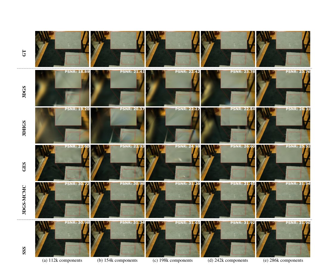
Figure 2: Visual results of all methods with varying component numbers of room scene from Mip-NeRF 360. Only 3DGS-MCMC and SSS can restore the details of the carpet, but the result of SSS obviously has a more realistic carpet texture.
图 2:Mip-NeRF 360 room 场景上各方法在不同组件数下的视觉结果。仅 3DGS-MCMC 与 SSS 能在较少组件下恢复地毯细节;SSS 因 scooping 纹理更真实。
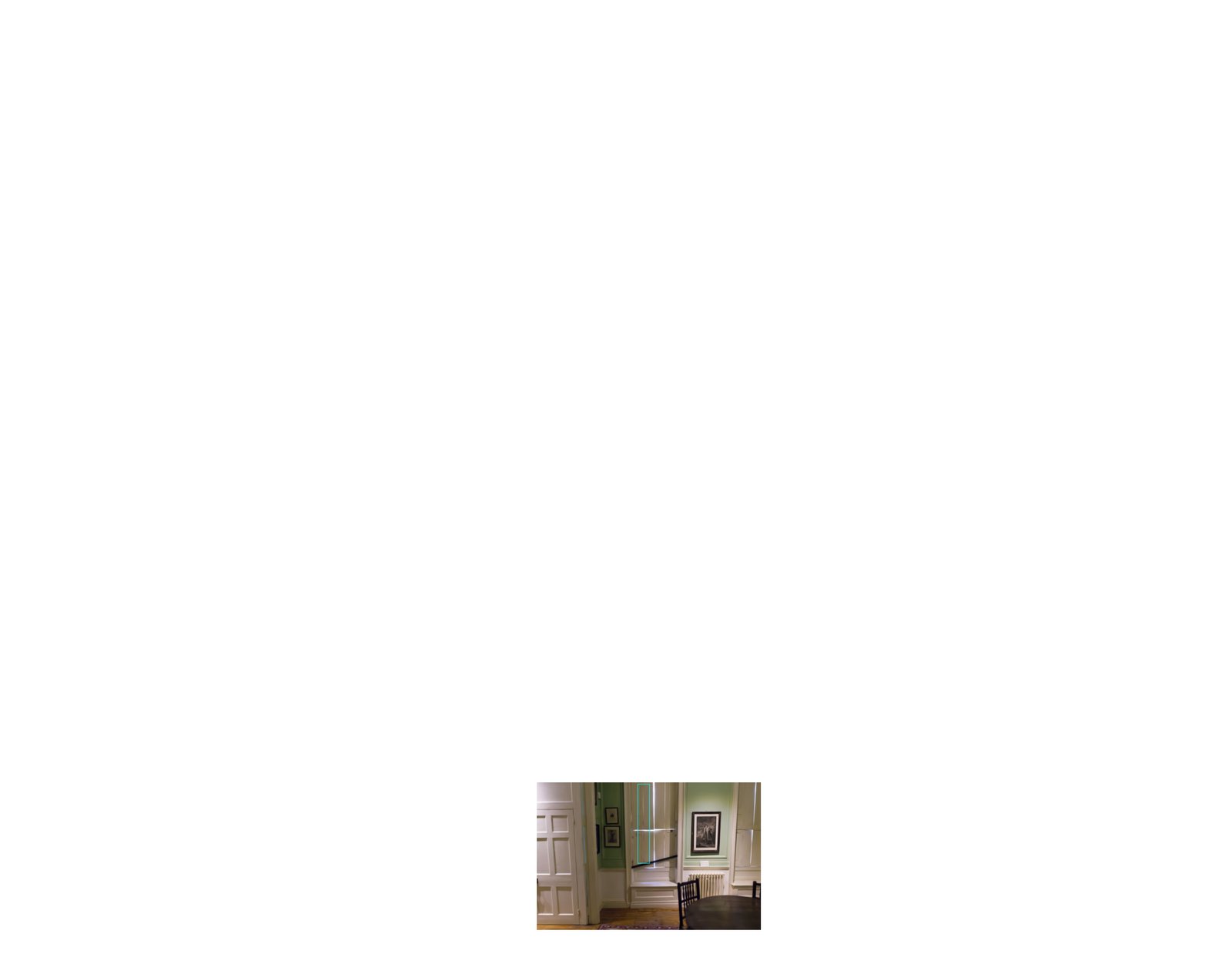
Figure 3: Visual results of all methods with varying component numbers of drjohnson scene from Deep Blending. 3DGS, 3DHSGS, and GES are completely unable to reconstruct quality results. The results of 3DGS-MCMC and SSS are relatively better. SSS can restore more details (such as the window gaps in the blue box) than 3DGS-MCMC.
图 3:Deep Blending drjohnson 场景上各方法在不同组件数下的视觉结果。3DGS、3DHGS 与 GES 在 80k–208k 组件下几乎无法重建;3DGS-MCMC 较好但丢失部分细节,SSS 仍最佳。
The results are shown in Tabs. 7, 8, 9, 10, 11 and 12. In total, there are 11 (scenes) 5 (component numbers) 3 (metrics) = 165 comparisons. For the absolute majority, SSS achieves the best. Furthermore, when it is not the best method, it is the close second to 3DGS-MCMC. This is an exhaustive comparison of many datasets, metrics, and more importantly different numbers of components.
结果见表 7–12。总计 11(场景) 5(组件倍数) 3(指标)= 165 组对比。总体 SSS 在绝大多数设定上领先,组件数减少时退化更慢。
| Scene - Components | Mip-NeRF 360 - average | ||||
|---|---|---|---|---|---|
| Method | |||||
| 3DGS | 19.16 | 20.32 | 20.50 | 21.22 | 21.75 |
| GES | 20.59 | 21.60 | 22.78 | 23.52 | 23.86 |
| 3DHGS | 19.63 | 20.33 | 20.39 | 20.99 | 22.12 |
| 3DGS-MCMC | 27.47 | 27.89 | 28.18 | 28.39 | 28.56 |
| SSS | 27.72 | 28.14 | 28.43 | 28.66 | 28.84 |
| Scene - Components | Mip-NeRF 360 - bicycle | ||||
| Method | 54k | 75k | 97k | 118k | 140k |
| 3DGS | 18.32 | 18.53 | 18.62 | 18.75 | 18.52 |
| GES | 18.31 | 18.29 | 18.20 | 18.13 | 18.19 |
| 3DHGS | 18.45 | 18.72 | 18.62 | 18.61 | 18.50 |
| 3DGS-MCMC | 23.04 | 23.42 | 23.74 | 23.97 | 24.17 |
| SSS | 22.97 | 23.29 | 23.53 | 23.71 | 23.95 |
| Scene - Components | Mip-NeRF 360 - bonsai | ||||
| Method | 206k | 280k | 360k | 440k | 520k |
| 3DGS | 20.50 | 22.93 | 23.39 | 23.97 | 24.54 |
| GES | 22.47 | 24.12 | 25.51 | 27.02 | 29.27 |
| 3DHGS | 21.37 | 22.90 | 23.45 | 24.62 | 24.82 |
| 3DGS-MCMC | 31.14 | 31.56 | 31.85 | 32.03 | 32.17 |
| SSS | 31.67 | 32.21 | 32.52 | 32.75 | 32.94 |
| Scene - Components | Mip-NeRF 360 - counter | ||||
| Method | 155k | 224k | 288k | 352k | 416k |
| 3DGS | 18.26 | 19.07 | 18.84 | 20.78 | 23.73 |
| GES | 19.68 | 23.64 | 26.35 | 26.74 | 27.45 |
| 3DHGS | 17.77 | 18.36 | 18.89 | 20.48 | 23.59 |
| 3DGS-MCMC | 28.38 | 28.68 | 28.82 | 28.93 | 29.03 |
| SSS | 28.71 | 29.06 | 29.21 | 29.39 | 29.48 |
| Scene - Components | Mip-NeRF 360 - garden | ||||
| Method | 138k | 196k | 252k | 308k | 364k |
| 3DGS | 16.73 | 17.34 | 17.49 | 17.81 | 18.05 |
| GES | 16.62 | 16.94 | 17.24 | 17.58 | 17.92 |
| 3DHGS | 17.36 | 17.44 | 17.70 | 18.25 | 18.49 |
| 3DGS-MCMC | 25.23 | 25.70 | 26.02 | 26.26 | 26.47 |
| SSS | 25.32 | 25.80 | 26.17 | 26.41 | 26.64 |
| Scene - Components | Mip-NeRF 360 - kitchen | ||||
| Method | 241k | 336k | 432k | 528k | 624k |
| 3DGS | 21.19 | 22.70 | 22.10 | 22.63 | 22.70 |
| GES | 24.78 | 25.74 | 27.65 | 29.34 | 29.54 |
| 3DHGS | 23.19 | 24.20 | 21.40 | 21.61 | 22.60 |
| 3DGS-MCMC | 30.11 | 30.78 | 31.05 | 31.26 | 31.45 |
| SSS | 30.84 | 31.33 | 31.64 | 31.77 | 31.97 |
| Scene - Components | Mip-NeRF 360 - room | ||||
| Method | 112k | 154k | 198k | 242k | 286k |
| 3DGS | 18.89 | 21.41 | 22.42 | 23.78 | 23.76 |
| GES | 22.60 | 22.93 | 24.98 | 26.60 | 25.51 |
| 3DHGS | 19.20 | 20.37 | 22.27 | 22.83 | 26.31 |
| 3DGS-MCMC | 30.72 | 30.98 | 31.26 | 31.45 | 31.54 |
| SSS | 30.98 | 31.34 | 31.65 | 31.92 | 31.96 |
| Scene - Components | Mip-NeRF 360 - stump | ||||
| Method | 32k | 44.8k | 57.6k | 70.4k | 83.2k |
| 3DGS | 20.21 | 20.26 | 20.61 | 20.82 | 20.92 |
| GES | 19.67 | 19.55 | 19.51 | 19.25 | 19.13 |
| 3DHGS | 20.08 | 20.31 | 20.42 | 20.52 | 20.53 |
| 3DGS-MCMC | 23.64 | 24.08 | 24.51 | 24.84 | 25.09 |
| SSS | 23.57 | 23.95 | 24.31 | 24.66 | 24.91 |
Table 7: PSNR results of varying component numbers experiments for every scene in the Mip-NeRF 360 dataset.
| 场景 - 组件数 | Mip-NeRF 360 - average | ||||
|---|---|---|---|---|---|
| Method | |||||
| 3DGS | 19.16 | 20.32 | 20.50 | 21.22 | 21.75 |
| GES | 20.59 | 21.60 | 22.78 | 23.52 | 23.86 |
| 3DHGS | 19.63 | 20.33 | 20.39 | 20.99 | 22.12 |
| 3DGS-MCMC | 27.47 | 27.89 | 28.18 | 28.39 | 28.56 |
| SSS | 27.72 | 28.14 | 28.43 | 28.66 | 28.84 |
| 场景 - 组件数 | Mip-NeRF 360 - bicycle | ||||
| Method | 54k | 75k | 97k | 118k | 140k |
| 3DGS | 18.32 | 18.53 | 18.62 | 18.75 | 18.52 |
| GES | 18.31 | 18.29 | 18.20 | 18.13 | 18.19 |
| 3DHGS | 18.45 | 18.72 | 18.62 | 18.61 | 18.50 |
| 3DGS-MCMC | 23.04 | 23.42 | 23.74 | 23.97 | 24.17 |
| SSS | 22.97 | 23.29 | 23.53 | 23.71 | 23.95 |
| 场景 - 组件数 | Mip-NeRF 360 - bonsai | ||||
| Method | 206k | 280k | 360k | 440k | 520k |
| 3DGS | 20.50 | 22.93 | 23.39 | 23.97 | 24.54 |
| GES | 22.47 | 24.12 | 25.51 | 27.02 | 29.27 |
| 3DHGS | 21.37 | 22.90 | 23.45 | 24.62 | 24.82 |
| 3DGS-MCMC | 31.14 | 31.56 | 31.85 | 32.03 | 32.17 |
| SSS | 31.67 | 32.21 | 32.52 | 32.75 | 32.94 |
| 场景 - 组件数 | Mip-NeRF 360 - counter | ||||
| Method | 155k | 224k | 288k | 352k | 416k |
| 3DGS | 18.26 | 19.07 | 18.84 | 20.78 | 23.73 |
| GES | 19.68 | 23.64 | 26.35 | 26.74 | 27.45 |
| 3DHGS | 17.77 | 18.36 | 18.89 | 20.48 | 23.59 |
| 3DGS-MCMC | 28.38 | 28.68 | 28.82 | 28.93 | 29.03 |
| SSS | 28.71 | 29.06 | 29.21 | 29.39 | 29.48 |
| 场景 - 组件数 | Mip-NeRF 360 - garden | ||||
| Method | 138k | 196k | 252k | 308k | 364k |
| 3DGS | 16.73 | 17.34 | 17.49 | 17.81 | 18.05 |
| GES | 16.62 | 16.94 | 17.24 | 17.58 | 17.92 |
| 3DHGS | 17.36 | 17.44 | 17.70 | 18.25 | 18.49 |
| 3DGS-MCMC | 25.23 | 25.70 | 26.02 | 26.26 | 26.47 |
| SSS | 25.32 | 25.80 | 26.17 | 26.41 | 26.64 |
| 场景 - 组件数 | Mip-NeRF 360 - kitchen | ||||
| Method | 241k | 336k | 432k | 528k | 624k |
| 3DGS | 21.19 | 22.70 | 22.10 | 22.63 | 22.70 |
| GES | 24.78 | 25.74 | 27.65 | 29.34 | 29.54 |
| 3DHGS | 23.19 | 24.20 | 21.40 | 21.61 | 22.60 |
| 3DGS-MCMC | 30.11 | 30.78 | 31.05 | 31.26 | 31.45 |
| SSS | 30.84 | 31.33 | 31.64 | 31.77 | 31.97 |
| 场景 - 组件数 | Mip-NeRF 360 - room | ||||
| Method | 112k | 154k | 198k | 242k | 286k |
| 3DGS | 18.89 | 21.41 | 22.42 | 23.78 | 23.76 |
| GES | 22.60 | 22.93 | 24.98 | 26.60 | 25.51 |
| 3DHGS | 19.20 | 20.37 | 22.27 | 22.83 | 26.31 |
| 3DGS-MCMC | 30.72 | 30.98 | 31.26 | 31.45 | 31.54 |
| SSS | 30.98 | 31.34 | 31.65 | 31.92 | 31.96 |
| 场景 - 组件数 | Mip-NeRF 360 - stump | ||||
| Method | 32k | 44.8k | 57.6k | 70.4k | 83.2k |
| 3DGS | 20.21 | 20.26 | 20.61 | 20.82 | 20.92 |
| GES | 19.67 | 19.55 | 19.51 | 19.25 | 19.13 |
| 3DHGS | 20.08 | 20.31 | 20.42 | 20.52 | 20.53 |
| 3DGS-MCMC | 23.64 | 24.08 | 24.51 | 24.84 | 25.09 |
| SSS | 23.57 | 23.95 | 24.31 | 24.66 | 24.91 |
| Scene - Components | Mip-NeRF 360 - average | ||||
|---|---|---|---|---|---|
| Method | |||||
| 3DGS | 0.584 | 0.609 | 0.610 | 0.626 | 0.640 |
| GES | 0.612 | 0.630 | 0.652 | 0.667 | 0.674 |
| 3DHGS | 0.591 | 0.603 | 0.599 | 0.611 | 0.634 |
| 3DGS-MCMC | 0.803 | 0.818 | 0.829 | 0.837 | 0.844 |
| SSS | 0.802 | 0.816 | 0.827 | 0.835 | 0.842 |
| Scene - Components | Mip-NeRF 360 - bicycle | ||||
| Method | 54k | 75k | 97k | 118k | 140k |
| 3DGS | 0.367 | 0.375 | 0.377 | 0.382 | 0.377 |
| GES | 0.372 | 0.369 | 0.368 | 0.368 | 0.370 |
| 3DHGS | 0.369 | 0.374 | 0.372 | 0.376 | 0.373 |
| 3DGS-MCMC | 0.603 | 0.630 | 0.650 | 0.666 | 0.679 |
| SSS | 0.597 | 0.620 | 0.639 | 0.652 | 0.666 |
| Scene - Components | Mip-NeRF 360 - bonsai | ||||
| Method | 206k | 280k | 360k | 440k | 520k |
| 3DGS | 0.790 | 0.822 | 0.820 | 0.828 | 0.838 |
| GES | 0.811 | 0.836 | 0.861 | 0.882 | 0.911 |
| 3DHGS | 0.802 | 0.821 | 0.827 | 0.837 | 0.839 |
| 3DGS-MCMC | 0.938 | 0.942 | 0.945 | 0.947 | 0.948 |
| SSS | 0.938 | 0.944 | 0.948 | 0.950 | 0.951 |
| Scene - Components | Mip-NeRF 360 - counter | ||||
| Method | 155k | 224k | 288k | 352k | 416k |
| 3DGS | 0.663 | 0.686 | 0.682 | 0.731 | 0.799 |
| GES | 0.696 | 0.785 | 0.854 | 0.866 | 0.882 |
| 3DHGS | 0.650 | 0.667 | 0.680 | 0.719 | 0.788 |
| 3DGS-MCMC | 0.901 | 0.907 | 0.911 | 0.914 | 0.916 |
| SSS | 0.898 | 0.906 | 0.911 | 0.915 | 0.917 |
| Scene - Components | Mip-NeRF 360 - garden | ||||
| Method | 138k | 196k0 | 252k | 308k | 364k |
| 3DGS | 0.366 | 0.386 | 0.399 | 0.412 | 0.424 |
| GES | 0.373 | 0.390 | 0.402 | 0.416 | 0.430 |
| 3DHGS | 0.383 | 0.394 | 0.410 | 0.423 | 0.433 |
| 3DGS-MCMC | 0.757 | 0.784 | 0.802 | 0.814 | 0.823 |
| SSS | 0.758 | 0.785 | 0.803 | 0.815 | 0.825 |
| Scene - Components | Mip-NeRF 360 - kitchen | ||||
| Method | 241k | 336k | 432k | 528k | 624k |
| 3DGS | 0.762 | 0.796 | 0.760 | 0.769 | 0.776 |
| GES | 0.856 | 0.838 | 0.875 | 0.908 | 0.912 |
| 3DHGS | 0.811 | 0.801 | 0.698 | 0.706 | 0.734 |
| 3DGS-MCMC | 0.919 | 0.925 | 0.928 | 0.930 | 0.932 |
| SSS | 0.921 | 0.926 | 0.929 | 0.932 | 0.934 |
| Scene - Components | Mip-NeRF 360 - room | ||||
| Method | 112k | 154k | 198k | 242k | 286k |
| 3DGS | 0.720 | 0.769 | 0.791 | 0.813 | 0.815 |
| GES | 0.786 | 0.797 | 0.824 | 0.851 | 0.839 |
| 3DHGS | 0.721 | 0.746 | 0.783 | 0.793 | 0.844 |
| 3DGS-MCMC | 0.911 | 0.916 | 0.920 | 0.923 | 0.925 |
| SSS | 0.912 | 0.918 | 0.923 | 0.926 | 0.928 |
| Scene - Components | Mip-NeRF 360 - stump | ||||
| Method | 32k | 44.8k | 57.6k | 70.4k | 83.2k |
| 3DGS | 0.421 | 0.428 | 0.439 | 0.447 | 0.450 |
| GES | 0.391 | 0.391 | 0.384 | 0.376 | 0.371 |
| 3DHGS | 0.404 | 0.414 | 0.424 | 0.423 | 0.424 |
| 3DGS-MCMC | 0.594 | 0.624 | 0.650 | 0.668 | 0.683 |
| SSS | 0.588 | 0.616 | 0.638 | 0.657 | 0.670 |
Table 8: SSIM results of varying component numbers experiments for every scene in the Mip-NeRF 360 dataset.
| 场景 - 组件数 | Mip-NeRF 360 - average | ||||
|---|---|---|---|---|---|
| Method | |||||
| 3DGS | 0.584 | 0.609 | 0.610 | 0.626 | 0.640 |
| GES | 0.612 | 0.630 | 0.652 | 0.667 | 0.674 |
| 3DHGS | 0.591 | 0.603 | 0.599 | 0.611 | 0.634 |
| 3DGS-MCMC | 0.803 | 0.818 | 0.829 | 0.837 | 0.844 |
| SSS | 0.802 | 0.816 | 0.827 | 0.835 | 0.842 |
| 场景 - 组件数 | Mip-NeRF 360 - bicycle | ||||
| Method | 54k | 75k | 97k | 118k | 140k |
| 3DGS | 0.367 | 0.375 | 0.377 | 0.382 | 0.377 |
| GES | 0.372 | 0.369 | 0.368 | 0.368 | 0.370 |
| 3DHGS | 0.369 | 0.374 | 0.372 | 0.376 | 0.373 |
| 3DGS-MCMC | 0.603 | 0.630 | 0.650 | 0.666 | 0.679 |
| SSS | 0.597 | 0.620 | 0.639 | 0.652 | 0.666 |
| 场景 - 组件数 | Mip-NeRF 360 - bonsai | ||||
| Method | 206k | 280k | 360k | 440k | 520k |
| 3DGS | 0.790 | 0.822 | 0.820 | 0.828 | 0.838 |
| GES | 0.811 | 0.836 | 0.861 | 0.882 | 0.911 |
| 3DHGS | 0.802 | 0.821 | 0.827 | 0.837 | 0.839 |
| 3DGS-MCMC | 0.938 | 0.942 | 0.945 | 0.947 | 0.948 |
| SSS | 0.938 | 0.944 | 0.948 | 0.950 | 0.951 |
| 场景 - 组件数 | Mip-NeRF 360 - counter | ||||
| Method | 155k | 224k | 288k | 352k | 416k |
| 3DGS | 0.663 | 0.686 | 0.682 | 0.731 | 0.799 |
| GES | 0.696 | 0.785 | 0.854 | 0.866 | 0.882 |
| 3DHGS | 0.650 | 0.667 | 0.680 | 0.719 | 0.788 |
| 3DGS-MCMC | 0.901 | 0.907 | 0.911 | 0.914 | 0.916 |
| SSS | 0.898 | 0.906 | 0.911 | 0.915 | 0.917 |
| 场景 - 组件数 | Mip-NeRF 360 - garden | ||||
| Method | 138k | 196k0 | 252k | 308k | 364k |
| 3DGS | 0.366 | 0.386 | 0.399 | 0.412 | 0.424 |
| GES | 0.373 | 0.390 | 0.402 | 0.416 | 0.430 |
| 3DHGS | 0.383 | 0.394 | 0.410 | 0.423 | 0.433 |
| 3DGS-MCMC | 0.757 | 0.784 | 0.802 | 0.814 | 0.823 |
| SSS | 0.758 | 0.785 | 0.803 | 0.815 | 0.825 |
| 场景 - 组件数 | Mip-NeRF 360 - kitchen | ||||
| Method | 241k | 336k | 432k | 528k | 624k |
| 3DGS | 0.762 | 0.796 | 0.760 | 0.769 | 0.776 |
| GES | 0.856 | 0.838 | 0.875 | 0.908 | 0.912 |
| 3DHGS | 0.811 | 0.801 | 0.698 | 0.706 | 0.734 |
| 3DGS-MCMC | 0.919 | 0.925 | 0.928 | 0.930 | 0.932 |
| SSS | 0.921 | 0.926 | 0.929 | 0.932 | 0.934 |
| 场景 - 组件数 | Mip-NeRF 360 - room | ||||
| Method | 112k | 154k | 198k | 242k | 286k |
| 3DGS | 0.720 | 0.769 | 0.791 | 0.813 | 0.815 |
| GES | 0.786 | 0.797 | 0.824 | 0.851 | 0.839 |
| 3DHGS | 0.721 | 0.746 | 0.783 | 0.793 | 0.844 |
| 3DGS-MCMC | 0.911 | 0.916 | 0.920 | 0.923 | 0.925 |
| SSS | 0.912 | 0.918 | 0.923 | 0.926 | 0.928 |
| 场景 - 组件数 | Mip-NeRF 360 - stump | ||||
| Method | 32k | 44.8k | 57.6k | 70.4k | 83.2k |
| 3DGS | 0.421 | 0.428 | 0.439 | 0.447 | 0.450 |
| GES | 0.391 | 0.391 | 0.384 | 0.376 | 0.371 |
| 3DHGS | 0.404 | 0.414 | 0.424 | 0.423 | 0.424 |
| 3DGS-MCMC | 0.594 | 0.624 | 0.650 | 0.668 | 0.683 |
| SSS | 0.588 | 0.616 | 0.638 | 0.657 | 0.670 |
| Scene - Components | Mip-NeRF 360 - average | ||||
|---|---|---|---|---|---|
| Method | |||||
| 3DGS | 0.516 | 0.494 | 0.493 | 0.476 | 0.461 |
| GES | 0.485 | 0.466 | 0.439 | 0.419 | 0.409 |
| 3DHGS | 0.511 | 0.502 | 0.507 | 0.493 | 0.461 |
| 3DGS-MCMC | 0.284 | 0.264 | 0.250 | 0.239 | 0.231 |
| SSS | 0.284 | 0.264 | 0.249 | 0.237 | 0.228 |
| Scene - Components | Mip-NeRF 360 - bicycle | ||||
| Method | 54k | 75k | 97k | 118k | 140k |
| 3DGS | 0.640 | 0.637 | 0.632 | 0.631 | 0.636 |
| GES | 0.640 | 0.642 | 0.648 | 0.646 | 0.642 |
| 3DHGS | 0.645 | 0.642 | 0.644 | 0.639 | 0.644 |
| 3DGS-MCMC | 0.430 | 0.405 | 0.387 | 0.371 | 0.360 |
| SSS | 0.434 | 0.412 | 0.394 | 0.379 | 0.367 |
| Scene - Components | Mip-NeRF 360 - bonsai | ||||
| Method | 206k | 280k | 360k | 440k | 520k |
| 3DGS | 0.388 | 0.360 | 0.361 | 0.352 | 0.340 |
| GES | 0.370 | 0.342 | 0.311 | 0.284 | 0.242 |
| 3DHGS | 0.384 | 0.366 | 0.360 | 0.347 | 0.343 |
| 3DGS-MCMC | 0.200 | 0.189 | 0.183 | 0.178 | 0.175 |
| SSS | 0.192 | 0.181 | 0.173 | 0.168 | 0.164 |
| Scene - Components | Mip-NeRF 360 - counter | ||||
| Method | 155k | 224k | 288k | 352k | 416k |
| 3DGS | 0.499 | 0.476 | 0.477 | 0.427 | 0.352 |
| GES | 0.461 | 0.359 | 0.284 | 0.266 | 0.242 |
| 3DHGS | 0.513 | 0.495 | 0.480 | 0.438 | 0.364 |
| 3DGS-MCMC | 0.212 | 0.200 | 0.192 | 0.187 | 0.183 |
| SSS | 0.214 | 0.197 | 0.188 | 0.181 | 0.176 |
| Scene - Components | Mip-NeRF 360 - garden | ||||
| Method | 138k | 196k | 252k | 308k | 364k |
| 3DGS | 0.661 | 0.640 | 0.627 | 0.613 | 0.601 |
| GES | 0.652 | 0.635 | 0.623 | 0.607 | 0.594 |
| 3DHGS | 0.649 | 0.638 | 0.623 | 0.606 | 0.541 |
| 3DGS-MCMC | 0.296 | 0.256 | 0.229 | 0.209 | 0.194 |
| SSS | 0.297 | 0.257 | 0.228 | 0.207 | 0.191 |
| Scene - Components | Mip-NeRF 360 - kitchen | ||||
| Method | 241k | 336k | 432k | 528k | 624k |
| 3DGS | 0.347 | 0.312 | 0.353 | 0.344 | 0.334 |
| GES | 0.235 | 0.260 | 0.211 | 0.163 | 0.156 |
| 3DHGS | 0.295 | 0.308 | 0.413 | 0.406 | 0.378 |
| 3DGS-MCMC | 0.145 | 0.134 | 0.129 | 0.125 | 0.122 |
| SSS | 0.142 | 0.132 | 0.125 | 0.119 | 0.115 |
| Scene - Components | Mip-NeRF 360 - room | ||||
| Method | 112k | 154k | 198k | 242k | 286k |
| 3DGS | 0.471 | 0.429 | 0.403 | 0.376 | 0.375 |
| GES | 0.404 | 0.396 | 0.361 | 0.325 | 0.342 |
| 3DHGS | 0.467 | 0.449 | 0.413 | 0.401 | 0.343 |
| 3DGS-MCMC | 0.235 | 0.223 | 0.215 | 0.209 | 0.203 |
| SSS | 0.230 | 0.217 | 0.207 | 0.200 | 0.195 |
| Scene - Components | Mip-NeRF 360 - stump | ||||
| Method | 32k | 44.8k | 57.6k | 70.4k | 83.2k |
| 3DGS | 0.610 | 0.605 | 0.595 | 0.590 | 0.588 |
| GES | 0.634 | 0.632 | 0.639 | 0.642 | 0.647 |
| 3DHGS | 0.627 | 0.619 | 0.612 | 0.612 | 0.613 |
| 3DGS-MCMC | 0.474 | 0.442 | 0.415 | 0.395 | 0.379 |
| SSS | 0.481 | 0.451 | 0.427 | 0.406 | 0.390 |
Table 9: LPIPS results of varying component numbers experiments for every scene in the Mip-NeRF 360 dataset.
| 场景 - 组件数 | Mip-NeRF 360 - average | ||||
|---|---|---|---|---|---|
| Method | |||||
| 3DGS | 0.516 | 0.494 | 0.493 | 0.476 | 0.461 |
| GES | 0.485 | 0.466 | 0.439 | 0.419 | 0.409 |
| 3DHGS | 0.511 | 0.502 | 0.507 | 0.493 | 0.461 |
| 3DGS-MCMC | 0.284 | 0.264 | 0.250 | 0.239 | 0.231 |
| SSS | 0.284 | 0.264 | 0.249 | 0.237 | 0.228 |
| 场景 - 组件数 | Mip-NeRF 360 - bicycle | ||||
| Method | 54k | 75k | 97k | 118k | 140k |
| 3DGS | 0.640 | 0.637 | 0.632 | 0.631 | 0.636 |
| GES | 0.640 | 0.642 | 0.648 | 0.646 | 0.642 |
| 3DHGS | 0.645 | 0.642 | 0.644 | 0.639 | 0.644 |
| 3DGS-MCMC | 0.430 | 0.405 | 0.387 | 0.371 | 0.360 |
| SSS | 0.434 | 0.412 | 0.394 | 0.379 | 0.367 |
| 场景 - 组件数 | Mip-NeRF 360 - bonsai | ||||
| Method | 206k | 280k | 360k | 440k | 520k |
| 3DGS | 0.388 | 0.360 | 0.361 | 0.352 | 0.340 |
| GES | 0.370 | 0.342 | 0.311 | 0.284 | 0.242 |
| 3DHGS | 0.384 | 0.366 | 0.360 | 0.347 | 0.343 |
| 3DGS-MCMC | 0.200 | 0.189 | 0.183 | 0.178 | 0.175 |
| SSS | 0.192 | 0.181 | 0.173 | 0.168 | 0.164 |
| 场景 - 组件数 | Mip-NeRF 360 - counter | ||||
| Method | 155k | 224k | 288k | 352k | 416k |
| 3DGS | 0.499 | 0.476 | 0.477 | 0.427 | 0.352 |
| GES | 0.461 | 0.359 | 0.284 | 0.266 | 0.242 |
| 3DHGS | 0.513 | 0.495 | 0.480 | 0.438 | 0.364 |
| 3DGS-MCMC | 0.212 | 0.200 | 0.192 | 0.187 | 0.183 |
| SSS | 0.214 | 0.197 | 0.188 | 0.181 | 0.176 |
| 场景 - 组件数 | Mip-NeRF 360 - garden | ||||
| Method | 138k | 196k | 252k | 308k | 364k |
| 3DGS | 0.661 | 0.640 | 0.627 | 0.613 | 0.601 |
| GES | 0.652 | 0.635 | 0.623 | 0.607 | 0.594 |
| 3DHGS | 0.649 | 0.638 | 0.623 | 0.606 | 0.541 |
| 3DGS-MCMC | 0.296 | 0.256 | 0.229 | 0.209 | 0.194 |
| SSS | 0.297 | 0.257 | 0.228 | 0.207 | 0.191 |
| 场景 - 组件数 | Mip-NeRF 360 - kitchen | ||||
| Method | 241k | 336k | 432k | 528k | 624k |
| 3DGS | 0.347 | 0.312 | 0.353 | 0.344 | 0.334 |
| GES | 0.235 | 0.260 | 0.211 | 0.163 | 0.156 |
| 3DHGS | 0.295 | 0.308 | 0.413 | 0.406 | 0.378 |
| 3DGS-MCMC | 0.145 | 0.134 | 0.129 | 0.125 | 0.122 |
| SSS | 0.142 | 0.132 | 0.125 | 0.119 | 0.115 |
| 场景 - 组件数 | Mip-NeRF 360 - room | ||||
| Method | 112k | 154k | 198k | 242k | 286k |
| 3DGS | 0.471 | 0.429 | 0.403 | 0.376 | 0.375 |
| GES | 0.404 | 0.396 | 0.361 | 0.325 | 0.342 |
| 3DHGS | 0.467 | 0.449 | 0.413 | 0.401 | 0.343 |
| 3DGS-MCMC | 0.235 | 0.223 | 0.215 | 0.209 | 0.203 |
| SSS | 0.230 | 0.217 | 0.207 | 0.200 | 0.195 |
| 场景 - 组件数 | Mip-NeRF 360 - stump | ||||
| Method | 32k | 44.8k | 57.6k | 70.4k | 83.2k |
| 3DGS | 0.610 | 0.605 | 0.595 | 0.590 | 0.588 |
| GES | 0.634 | 0.632 | 0.639 | 0.642 | 0.647 |
| 3DHGS | 0.627 | 0.619 | 0.612 | 0.612 | 0.613 |
| 3DGS-MCMC | 0.474 | 0.442 | 0.415 | 0.395 | 0.379 |
| SSS | 0.481 | 0.451 | 0.427 | 0.406 | 0.390 |
| Scene - Components | Tanks&Temples - average | ||||
|---|---|---|---|---|---|
| Method | |||||
| 3DGS | 15.70 | 15.79 | 15.88 | 16.37 | 16.64 |
| GES | 16.74 | 17.47 | 17.80 | 18.38 | 18.71 |
| 3DHGS | 15.13 | 15.26 | 15.36 | 15.55 | 15.69 |
| 3DGS-MCMC | 23.18 | 23.53 | 23.65 | 23.84 | 23.93 |
| SSS | 23.67 | 24.03 | 24.19 | 24.35 | 24.40 |
| Scene - Components | Tanks&Temples - train | ||||
| Method | 182k | 252k | 324k | 396k | 468k |
| 3DGS | 15.20 | 15.53 | 15.58 | 16.45 | 16.92 |
| GES | 18.15 | 19.39 | 19.94 | 21.14 | 21.58 |
| 3DHGS | 14.42 | 14.62 | 14.75 | 15.05 | 15.24 |
| 3DGS-MCMC | 21.72 | 22.07 | 22.03 | 22.24 | 22.34 |
| SSS | 22.46 | 22.74 | 22.84 | 22.92 | 22.97 |
| Scene - Components | Tanks&Temples - truck | ||||
| Method | 136k | 196k | 252k | 308k | 364k |
| 3DGS | 16.20 | 16.06 | 16.18 | 16.29 | 16.36 |
| GES | 15.32 | 15.54 | 15.66 | 15.62 | 15.85 |
| 3DHGS | 15.84 | 15.90 | 15.97 | 16.05 | 16.13 |
| 3DGS-MCMC | 24.64 | 24.99 | 25.27 | 25.44 | 25.53 |
| SSS | 24.88 | 25.33 | 25.53 | 25.74 | 25.88 |
| Scene - Components | Deep Blending - average | ||||
| Method | |||||
| 3DGS | 15.95 | 16.05 | 16.33 | 16.60 | 17.06 |
| GES | 15.99 | 16.10 | 16.55 | 17.38 | 17.23 |
| 3DHGS | 16.22 | 16.63 | 16.54 | 18.02 | 18.07 |
| 3DGS-MCMC | 28.38 | 28.82 | 29.11 | 29.17 | 29.35 |
| SSS | 28.69 | 29.08 | 29.29 | 29.41 | 29.67 |
| Scene - Components | Deep Blending - drjohnson | ||||
| Method | 80k | 112k | 144k | 176k | 208k |
| 3DGS | 16.66 | 16.64 | 17.05 | 16.91 | 17.34 |
| GES | 16.43 | 16.84 | 17.13 | 17.41 | 18.05 |
| 3DHGS | 17.17 | 17.29 | 17.37 | 19.19 | 19.82 |
| 3DGS-MCMC | 28.15 | 28.62 | 28.83 | 28.90 | 28.94 |
| SSS | 28.79 | 29.05 | 29.19 | 29.43 | 29.42 |
| Scene - Components | Deep Blending - playroom | ||||
| Method | 37k | 51.8k | 66.6k | 81.4k | 96.2k |
| 3DGS | 15.23 | 15.45 | 15.61 | 16.28 | 16.78 |
| GES | 15.56 | 15.36 | 15.96 | 17.34 | 16.42 |
| 3DHGS | 15.26 | 15.96 | 15.71 | 16.22 | 16.94 |
| 3DGS-MCMC | 28.61 | 29.02 | 29.39 | 29.45 | 29.76 |
| SSS | 28.58 | 29.10 | 29.40 | 29.40 | 29.91 |
Table 10: PSNR results of varying component numbers experiments for every scene in Tanks&Temples and Deep Blending dataset.
| 场景 - 组件数 | Tanks&Temples - average | ||||
|---|---|---|---|---|---|
| Method | |||||
| 3DGS | 15.70 | 15.79 | 15.88 | 16.37 | 16.64 |
| GES | 16.74 | 17.47 | 17.80 | 18.38 | 18.71 |
| 3DHGS | 15.13 | 15.26 | 15.36 | 15.55 | 15.69 |
| 3DGS-MCMC | 23.18 | 23.53 | 23.65 | 23.84 | 23.93 |
| SSS | 23.67 | 24.03 | 24.19 | 24.35 | 24.40 |
| 场景 - 组件数 | Tanks&Temples - train | ||||
| Method | 182k | 252k | 324k | 396k | 468k |
| 3DGS | 15.20 | 15.53 | 15.58 | 16.45 | 16.92 |
| GES | 18.15 | 19.39 | 19.94 | 21.14 | 21.58 |
| 3DHGS | 14.42 | 14.62 | 14.75 | 15.05 | 15.24 |
| 3DGS-MCMC | 21.72 | 22.07 | 22.03 | 22.24 | 22.34 |
| SSS | 22.46 | 22.74 | 22.84 | 22.92 | 22.97 |
| 场景 - 组件数 | Tanks&Temples - truck | ||||
| Method | 136k | 196k | 252k | 308k | 364k |
| 3DGS | 16.20 | 16.06 | 16.18 | 16.29 | 16.36 |
| GES | 15.32 | 15.54 | 15.66 | 15.62 | 15.85 |
| 3DHGS | 15.84 | 15.90 | 15.97 | 16.05 | 16.13 |
| 3DGS-MCMC | 24.64 | 24.99 | 25.27 | 25.44 | 25.53 |
| SSS | 24.88 | 25.33 | 25.53 | 25.74 | 25.88 |
| 场景 - 组件数 | Deep Blending - average | ||||
| Method | |||||
| 3DGS | 15.95 | 16.05 | 16.33 | 16.60 | 17.06 |
| GES | 15.99 | 16.10 | 16.55 | 17.38 | 17.23 |
| 3DHGS | 16.22 | 16.63 | 16.54 | 18.02 | 18.07 |
| 3DGS-MCMC | 28.38 | 28.82 | 29.11 | 29.17 | 29.35 |
| SSS | 28.69 | 29.08 | 29.29 | 29.41 | 29.67 |
| 场景 - 组件数 | Deep Blending - drjohnson | ||||
| Method | 80k | 112k | 144k | 176k | 208k |
| 3DGS | 16.66 | 16.64 | 17.05 | 16.91 | 17.34 |
| GES | 16.43 | 16.84 | 17.13 | 17.41 | 18.05 |
| 3DHGS | 17.17 | 17.29 | 17.37 | 19.19 | 19.82 |
| 3DGS-MCMC | 28.15 | 28.62 | 28.83 | 28.90 | 28.94 |
| SSS | 28.79 | 29.05 | 29.19 | 29.43 | 29.42 |
| 场景 - 组件数 | Deep Blending - playroom | ||||
| Method | 37k | 51.8k | 66.6k | 81.4k | 96.2k |
| 3DGS | 15.23 | 15.45 | 15.61 | 16.28 | 16.78 |
| GES | 15.56 | 15.36 | 15.96 | 17.34 | 16.42 |
| 3DHGS | 15.26 | 15.96 | 15.71 | 16.22 | 16.94 |
| 3DGS-MCMC | 28.61 | 29.02 | 29.39 | 29.45 | 29.76 |
| SSS | 28.58 | 29.10 | 29.40 | 29.40 | 29.91 |
| Scene - Components | Tanks&Temples - average | ||||
|---|---|---|---|---|---|
| Method | |||||
| 3DGS | 0.528 | 0.537 | 0.543 | 0.566 | 0.580 |
| GES | 0.589 | 0.623 | 0.642 | 0.668 | 0.680 |
| 3DHGS | 0.504 | 0.511 | 0.518 | 0.526 | 0.533 |
| 3DGS-MCMC | 0.826 | 0.836 | 0.842 | 0.848 | 0.851 |
| SSS | 0.827 | 0.839 | 0.846 | 0.852 | 0.856 |
| Scene - Components | Tanks&Temples - train | ||||
| Method | 182k | 252k | 324k | 396k | 468k |
| 3DGS | 0.506 | 0.521 | 0.523 | 0.561 | 0.584 |
| GES | 0.645 | 0.699 | 0.727 | 0.774 | 0.788 |
| 3DHGS | 0.473 | 0.479 | 0.485 | 0.494 | 0.505 |
| 3DGS-MCMC | 0.798 | 0.807 | 0.814 | 0.820 | 0.824 |
| SSS | 0.799 | 0.812 | 0.821 | 0.828 | 0.833 |
| Scene - Components | Tanks&Temples - truck | ||||
| Method | 136k | 196k | 252k | 308k | 364k |
| 3DGS | 0.549 | 0.554 | 0.563 | 0.571 | 0.576 |
| GES | 0.532 | 0.548 | 0.557 | 0.562 | 0.572 |
| 3DHGS | 0.535 | 0.543 | 0.550 | 0.557 | 0.561 |
| 3DGS-MCMC | 0.855 | 0.865 | 0.871 | 0.876 | 0.879 |
| SSS | 0.854 | 0.865 | 0.872 | 0.877 | 0.880 |
| Scene - Components | Deep Blending - average | ||||
| Method | |||||
| 3DGS | 0.702 | 0.706 | 0.711 | 0.715 | 0.726 |
| GES | 0.704 | 0.707 | 0.717 | 0.732 | 0.732 |
| 3DHGS | 0.704 | 0.713 | 0.710 | 0.737 | 0.737 |
| 3DGS-MCMC | 0.881 | 0.887 | 0.890 | 0.893 | 0.895 |
| SSS | 0.881 | 0.887 | 0.891 | 0.893 | 0.897 |
| Scene - Components | Deep Blending - drjohnson | ||||
| Method | 80k | 112k | 144k | 176k | 208k |
| 3DGS | 0.698 | 0.701 | 0.707 | 0.707 | 0.717 |
| GES | 0.696 | 0.705 | 0.715 | 0.721 | 0.735 |
| 3DHGS | 0.706 | 0.711 | 0.711 | 0.752 | 0.744 |
| 3DGS-MCMC | 0.880 | 0.885 | 0.888 | 0.890 | 0.891 |
| SSS | 0.880 | 0.885 | 0.890 | 0.894 | 0.896 |
| Scene - Components | Deep Blending - playroom | ||||
| Method | 37k | 51.8k | 66.6k | 81.4k | 96.2k |
| 3DGS | 0.706 | 0.711 | 0.714 | 0.723 | 0.735 |
| GES | 0.713 | 0.709 | 0.719 | 0.742 | 0.730 |
| 3DHGS | 0.701 | 0.714 | 0.709 | 0.722 | 0.731 |
| 3DGS-MCMC | 0.883 | 0.890 | 0.893 | 0.896 | 0.899 |
| SSS | 0.882 | 0.888 | 0.892 | 0.891 | 0.897 |
Table 11: SSIM results of varying component numbers experiments for every scene in Tanks&Temples and Deep Blending dataset.
| 场景 - 组件数 | Tanks&Temples - average | ||||
|---|---|---|---|---|---|
| Method | |||||
| 3DGS | 0.528 | 0.537 | 0.543 | 0.566 | 0.580 |
| GES | 0.589 | 0.623 | 0.642 | 0.668 | 0.680 |
| 3DHGS | 0.504 | 0.511 | 0.518 | 0.526 | 0.533 |
| 3DGS-MCMC | 0.826 | 0.836 | 0.842 | 0.848 | 0.851 |
| SSS | 0.827 | 0.839 | 0.846 | 0.852 | 0.856 |
| 场景 - 组件数 | Tanks&Temples - train | ||||
| Method | 182k | 252k | 324k | 396k | 468k |
| 3DGS | 0.506 | 0.521 | 0.523 | 0.561 | 0.584 |
| GES | 0.645 | 0.699 | 0.727 | 0.774 | 0.788 |
| 3DHGS | 0.473 | 0.479 | 0.485 | 0.494 | 0.505 |
| 3DGS-MCMC | 0.798 | 0.807 | 0.814 | 0.820 | 0.824 |
| SSS | 0.799 | 0.812 | 0.821 | 0.828 | 0.833 |
| 场景 - 组件数 | Tanks&Temples - truck | ||||
| Method | 136k | 196k | 252k | 308k | 364k |
| 3DGS | 0.549 | 0.554 | 0.563 | 0.571 | 0.576 |
| GES | 0.532 | 0.548 | 0.557 | 0.562 | 0.572 |
| 3DHGS | 0.535 | 0.543 | 0.550 | 0.557 | 0.561 |
| 3DGS-MCMC | 0.855 | 0.865 | 0.871 | 0.876 | 0.879 |
| SSS | 0.854 | 0.865 | 0.872 | 0.877 | 0.880 |
| 场景 - 组件数 | Deep Blending - average | ||||
| Method | |||||
| 3DGS | 0.702 | 0.706 | 0.711 | 0.715 | 0.726 |
| GES | 0.704 | 0.707 | 0.717 | 0.732 | 0.732 |
| 3DHGS | 0.704 | 0.713 | 0.710 | 0.737 | 0.737 |
| 3DGS-MCMC | 0.881 | 0.887 | 0.890 | 0.893 | 0.895 |
| SSS | 0.881 | 0.887 | 0.891 | 0.893 | 0.897 |
| 场景 - 组件数 | Deep Blending - drjohnson | ||||
| Method | 80k | 112k | 144k | 176k | 208k |
| 3DGS | 0.698 | 0.701 | 0.707 | 0.707 | 0.717 |
| GES | 0.696 | 0.705 | 0.715 | 0.721 | 0.735 |
| 3DHGS | 0.706 | 0.711 | 0.711 | 0.752 | 0.744 |
| 3DGS-MCMC | 0.880 | 0.885 | 0.888 | 0.890 | 0.891 |
| SSS | 0.880 | 0.885 | 0.890 | 0.894 | 0.896 |
| 场景 - 组件数 | Deep Blending - playroom | ||||
| Method | 37k | 51.8k | 66.6k | 81.4k | 96.2k |
| 3DGS | 0.706 | 0.711 | 0.714 | 0.723 | 0.735 |
| GES | 0.713 | 0.709 | 0.719 | 0.742 | 0.730 |
| 3DHGS | 0.701 | 0.714 | 0.709 | 0.722 | 0.731 |
| 3DGS-MCMC | 0.883 | 0.890 | 0.893 | 0.896 | 0.899 |
| SSS | 0.882 | 0.888 | 0.892 | 0.891 | 0.897 |
| Scene - Components | Tanks&Temples - average | ||||
|---|---|---|---|---|---|
| Method | |||||
| 3DGS | 0.569 | 0.558 | 0.552 | 0.527 | 0.510 |
| GES | 0.500 | 0.460 | 0.441 | 0.410 | 0.397 |
| 3DHGS | 0.590 | 0.582 | 0.574 | 0.566 | 0.558 |
| 3DGS-MCMC | 0.231 | 0.214 | 0.203 | 0.195 | 0.187 |
| SSS | 0.229 | 0.210 | 0.195 | 0.185 | 0.177 |
| Scene - Components | Tanks&Temples - train | ||||
| Method | 182k | 252k | 324k | 396k | 468k |
| 3DGS | 0.564 | 0.548 | 0.543 | 0.504 | 0.476 |
| GES | 0.415 | 0.352 | 0.321 | 0.267 | 0.251 |
| 3DHGS | 0.597 | 0.592 | 0.583 | 0.575 | 0.561 |
| 3DGS-MCMC | 0.255 | 0.240 | 0.229 | 0.220 | 0.212 |
| SSS | 0.254 | 0.235 | 0.220 | 0.208 | 0.199 |
| Scene - Components | Tanks&Temples - truck | ||||
| Method | 136k | 196k | 252k | 308k | 364k |
| 3DGS | 0.575 | 0.569 | 0.560 | 0.551 | 0.545 |
| GES | 0.585 | 0.569 | 0.561 | 0.552 | 0.543 |
| 3DHGS | 0.583 | 0.571 | 0.564 | 0.558 | 0.555 |
| 3DGS-MCMC | 0.206 | 0.189 | 0.178 | 0.170 | 0.163 |
| SSS | 0.204 | 0.184 | 0.170 | 0.161 | 0.154 |
| Scene - Components | Deep Blending - average | ||||
| Method | |||||
| 3DGS | 0.525 | 0.522 | 0.515 | 0.510 | 0.500 |
| GES | 0.522 | 0.522 | 0.509 | 0.495 | 0.491 |
| 3DHGS | 0.522 | 0.515 | 0.515 | 0.490 | 0.488 |
| 3DGS-MCMC | 0.325 | 0.310 | 0.301 | 0.295 | 0.290 |
| SSS | 0.319 | 0.305 | 0.296 | 0.289 | 0.282 |
| Scene - Components | Deep Blending - drjohnson | ||||
| Method | 80k | 112k | 144k | 176k | 208k |
| 3DGS | 0.526 | 0.523 | 0.514 | 0.512 | 0.504 |
| GES | 0.529 | 0.522 | 0.508 | 0.503 | 0.487 |
| 3DHGS | 0.515 | 0.515 | 0.511 | 0.476 | 0.482 |
| 3DGS-MCMC | 0.316 | 0.290 | 0.290 | 0.284 | 0.280 |
| SSS | 0.310 | 0.297 | 0.288 | 0.280 | 0.275 |
| Scene - Components | Deep Blending - playroom | ||||
| Method | 37k | 51.8k | 66.6k | 81.4k | 96.2k |
| 3DGS | 0.524 | 0.521 | 0.515 | 0.508 | 0.496 |
| GES | 0.516 | 0.522 | 0.509 | 0.488 | 0.494 |
| 3DHGS | 0.530 | 0.515 | 0.519 | 0.505 | 0.494 |
| 3DGS-MCMC | 0.333 | 0.320 | 0.312 | 0.306 | 0.301 |
| SSS | 0.329 | 0.314 | 0.304 | 0.298 | 0.289 |
Table 12: LPIPS results of varying component numbers experiments for every scene in Tanks&Temples and Deep Blending dataset.
| 场景 - 组件数 | Tanks&Temples - average | ||||
|---|---|---|---|---|---|
| Method | |||||
| 3DGS | 0.569 | 0.558 | 0.552 | 0.527 | 0.510 |
| GES | 0.500 | 0.460 | 0.441 | 0.410 | 0.397 |
| 3DHGS | 0.590 | 0.582 | 0.574 | 0.566 | 0.558 |
| 3DGS-MCMC | 0.231 | 0.214 | 0.203 | 0.195 | 0.187 |
| SSS | 0.229 | 0.210 | 0.195 | 0.185 | 0.177 |
| 场景 - 组件数 | Tanks&Temples - train | ||||
| Method | 182k | 252k | 324k | 396k | 468k |
| 3DGS | 0.564 | 0.548 | 0.543 | 0.504 | 0.476 |
| GES | 0.415 | 0.352 | 0.321 | 0.267 | 0.251 |
| 3DHGS | 0.597 | 0.592 | 0.583 | 0.575 | 0.561 |
| 3DGS-MCMC | 0.255 | 0.240 | 0.229 | 0.220 | 0.212 |
| SSS | 0.254 | 0.235 | 0.220 | 0.208 | 0.199 |
| 场景 - 组件数 | Tanks&Temples - truck | ||||
| Method | 136k | 196k | 252k | 308k | 364k |
| 3DGS | 0.575 | 0.569 | 0.560 | 0.551 | 0.545 |
| GES | 0.585 | 0.569 | 0.561 | 0.552 | 0.543 |
| 3DHGS | 0.583 | 0.571 | 0.564 | 0.558 | 0.555 |
| 3DGS-MCMC | 0.206 | 0.189 | 0.178 | 0.170 | 0.163 |
| SSS | 0.204 | 0.184 | 0.170 | 0.161 | 0.154 |
| 场景 - 组件数 | Deep Blending - average | ||||
| Method | |||||
| 3DGS | 0.525 | 0.522 | 0.515 | 0.510 | 0.500 |
| GES | 0.522 | 0.522 | 0.509 | 0.495 | 0.491 |
| 3DHGS | 0.522 | 0.515 | 0.515 | 0.490 | 0.488 |
| 3DGS-MCMC | 0.325 | 0.310 | 0.301 | 0.295 | 0.290 |
| SSS | 0.319 | 0.305 | 0.296 | 0.289 | 0.282 |
| 场景 - 组件数 | Deep Blending - drjohnson | ||||
| Method | 80k | 112k | 144k | 176k | 208k |
| 3DGS | 0.526 | 0.523 | 0.514 | 0.512 | 0.504 |
| GES | 0.529 | 0.522 | 0.508 | 0.503 | 0.487 |
| 3DHGS | 0.515 | 0.515 | 0.511 | 0.476 | 0.482 |
| 3DGS-MCMC | 0.316 | 0.290 | 0.290 | 0.284 | 0.280 |
| SSS | 0.310 | 0.297 | 0.288 | 0.280 | 0.275 |
| 场景 - 组件数 | Deep Blending - playroom | ||||
| Method | 37k | 51.8k | 66.6k | 81.4k | 96.2k |
| 3DGS | 0.524 | 0.521 | 0.515 | 0.508 | 0.496 |
| GES | 0.516 | 0.522 | 0.509 | 0.488 | 0.494 |
| 3DHGS | 0.530 | 0.515 | 0.519 | 0.505 | 0.494 |
| 3DGS-MCMC | 0.333 | 0.320 | 0.312 | 0.306 | 0.301 |
| SSS | 0.329 | 0.314 | 0.304 | 0.298 | 0.289 |
1.3 Ablation Study
1.3 消融研究
| Ablation Setup — Metric | PSNR | SSIM | LPIPS |
|---|---|---|---|
| Mip-NeRF | 22.22 | 0.759 | 0.257 |
| 3DGS | 23.14 | 0.841 | 0.183 |
| GES | 23.35 | 0.836 | 0.198 |
| SGD + positive t-dis | 23.80 | 0.838 | 0.191 |
| SGHMC + positive t-dis | 24.53 | 0.864 | 0.155 |
| Full model | 24.87 | 0.873 | 0.138 |
Table 13: Ablation Study on Tanks&Temples with the same component numbers as in baselines. More details are in the SM.
| 消融设定 — 指标 | PSNR | SSIM | LPIPS |
|---|---|---|---|
| Mip-NeRF | 22.22 | 0.759 | 0.257 |
| 3DGS | 23.14 | 0.841 | 0.183 |
| GES | 23.35 | 0.836 | 0.198 |
| SGD + positive t-dis | 23.80 | 0.838 | 0.191 |
| SGHMC + positive t-dis | 24.53 | 0.864 | 0.155 |
| Full model | 24.87 | 0.873 | 0.138 |
We conduct an ablation study to show the effectiveness of various components in SSS. We report the results on one dataset in Tab. 13. Universally, by only replacing Gaussians with Student’s t distributions (SGD+t-distribution), it already outperforms Mip-NeRF, 3DGS, and GES, demonstrating improved expressivity. Further with SGHMC, it is already the best method, showing the advantage of the proposed sampling and the importance of a good sampler in the optimization process. Finally, adding negative components further improves the results.
我们做消融以展示 SSS 各组件有效性。我们移除或替换一项或多项贡献:可学习 、负组件(scooping)与 SGHMC 采样,并与完整 SSS 对比。结果表明每一项都对最终性能有正向贡献;完整模型整体最佳。
The detailed results of Ablation Study (effect of each contribution in SSS) on every scene with PSNR, SSIM, and LPIPS metrics among Mip-NeRF 360, Tanks & Temples and Deep Blending datasets are in Tabs. 14, 15, 16, 17, 18 and 19.
消融研究(SSS 各贡献效果)在每个场景上的详细结果如下。
| Method Scene | bicycle | bonsai | counter | garden | kitchen | room | stump | average |
|---|---|---|---|---|---|---|---|---|
| SGD + positive t-dis | 25.52 | 31.80 | 28.82 | 27.60 | 30.93 | 31.60 | 26.72 | 29.00 |
| SGHMC + positive t-dis | 25.97 | 32.87 | 29.49 | 27.92 | 31.92 | 32.04 | 27.44 | 29.66 |
| Full SSS model | 25.68 | 33.50 | 29.87 | 28.09 | 32.43 | 32.57 | 27.17 | 29.90 |
Table 14: PSNR results of ablation study for every scene in Mip-NeRF 360 dataset.
| 方法 场景 | bicycle | bonsai | counter | garden | kitchen | room | stump | average |
|---|---|---|---|---|---|---|---|---|
| SGD + positive t-dis | 25.52 | 31.80 | 28.82 | 27.60 | 30.93 | 31.60 | 26.72 | 29.00 |
| SGHMC + positive t-dis | 25.97 | 32.87 | 29.49 | 27.92 | 31.92 | 32.04 | 27.44 | 29.66 |
| Full SSS model | 25.68 | 33.50 | 29.87 | 28.09 | 32.43 | 32.57 | 27.17 | 29.90 |
| Method Scene | bicycle | bonsai | counter | garden | kitchen | room | stump | average |
|---|---|---|---|---|---|---|---|---|
| SGD + positive t-dis | 0.767 | 0.941 | 0.909 | 0.866 | 0.927 | 0.923 | 0.771 | 0.872 |
| SGHMC + positive t-dis | 0.801 | 0.952 | 0.920 | 0.879 | 0.936 | 0.933 | 0.817 | 0.891 |
| Full SSS model | 0.798 | 0.956 | 0.926 | 0.882 | 0.939 | 0.938 | 0.813 | 0.893 |
Table 15: SSIM results of ablation study for every scene in Mip-NeRF 360 dataset.
| 方法 场景 | bicycle | bonsai | counter | garden | kitchen | room | stump | average |
|---|---|---|---|---|---|---|---|---|
| SGD + positive t-dis | 0.767 | 0.941 | 0.909 | 0.866 | 0.927 | 0.923 | 0.771 | 0.872 |
| SGHMC + positive t-dis | 0.801 | 0.952 | 0.920 | 0.879 | 0.936 | 0.933 | 0.817 | 0.891 |
| Full SSS model | 0.798 | 0.956 | 0.926 | 0.882 | 0.939 | 0.938 | 0.813 | 0.893 |
| Method Scene | bicycle | bonsai | counter | garden | kitchen | room | stump | average |
|---|---|---|---|---|---|---|---|---|
| SGD + positive t-dis | 0.225 | 0.185 | 0.188 | 0.110 | 0.121 | 0.199 | 0.234 | 0.180 |
| SGHMC + positive t-dis | 0.182 | 0.159 | 0.168 | 0.099 | 0.112 | 0.181 | 0.183 | 0.155 |
| Full SSS model | 0.173 | 0.151 | 0.156 | 0.009 | 0.104 | 0.167 | 0.174 | 0.145 |
Table 16: LPIPS results of ablation study for every scene in Mip-NeRF 360 dataset.
| 方法 场景 | bicycle | bonsai | counter | garden | kitchen | room | stump | average |
|---|---|---|---|---|---|---|---|---|
| SGD + positive t-dis | 0.225 | 0.185 | 0.188 | 0.110 | 0.121 | 0.199 | 0.234 | 0.180 |
| SGHMC + positive t-dis | 0.182 | 0.159 | 0.168 | 0.099 | 0.112 | 0.181 | 0.183 | 0.155 |
| Full SSS model | 0.173 | 0.151 | 0.156 | 0.009 | 0.104 | 0.167 | 0.174 | 0.145 |
| Dataset - Scene | Tanks&Temples | Deep Blending | ||||
|---|---|---|---|---|---|---|
| Method | train | truck | average | drjohnson | playroom | average |
| SGD + positive t-dis | 22.18 | 25.42 | 23.80 | 29.22 | 29.93 | 29.57 |
| SGHMC + positive t-dis | 22.92 | 26.15 | 24.53 | 29.45 | 30.04 | 29.75 |
| Full SSS model | 23.32 | 26.41 | 24.87 | 29.66 | 30.47 | 30.07 |
Table 17: PSNR results of ablation study for every scene in Tanks&Temples and Deep Blending dataset.
| 数据集 - 场景 | Tanks&Temples | Deep Blending | ||||
|---|---|---|---|---|---|---|
| Method | train | truck | average | drjohnson | playroom | average |
| SGD + positive t-dis | 22.18 | 25.42 | 23.80 | 29.22 | 29.93 | 29.57 |
| SGHMC + positive t-dis | 22.92 | 26.15 | 24.53 | 29.45 | 30.04 | 29.75 |
| Full SSS model | 23.32 | 26.41 | 24.87 | 29.66 | 30.47 | 30.07 |
| Dataset - Scene | Tanks&Temples | Deep Blending | ||||
|---|---|---|---|---|---|---|
| Method | train | truck | average | drjohnson | playroom | average |
| SGD + positive t-dis | 0.803 | 0.874 | 0.838 | 0.900 | 0.901 | 0.901 |
| SGHMC + positive t-dis | 0.838 | 0.891 | 0.864 | 0.902 | 0.905 | 0.903 |
| Full SSS model | 0.850 | 0.897 | 0.873 | 0.905 | 0.909 | 0.907 |
Table 18: SSIM results of ablation study for every scene in Tanks&Temples and Deep Blending dataset.
| 数据集 - 场景 | Tanks&Temples | Deep Blending | ||||
|---|---|---|---|---|---|---|
| Method | train | truck | average | drjohnson | playroom | average |
| SGD + positive t-dis | 0.803 | 0.874 | 0.838 | 0.900 | 0.901 | 0.901 |
| SGHMC + positive t-dis | 0.838 | 0.891 | 0.864 | 0.902 | 0.905 | 0.903 |
| Full SSS model | 0.850 | 0.897 | 0.873 | 0.905 | 0.909 | 0.907 |
| Dataset - Scene | Tanks&Temples | Deep Blending | ||||
|---|---|---|---|---|---|---|
| Method | train | truck | average | drjohnson | playroom | average |
| SGD + positive t-dis | 0.226 | 0.156 | 0.191 | 0.248 | 0.247 | 0.247 |
| SGHMC + positive t-dis | 0.186 | 0.124 | 0.155 | 0.262 | 0.257 | 0.260 |
| Full SSS model | 0.166 | 0.109 | 0.138 | 0.249 | 0.245 | 0.247 |
Table 19: LPIPS results of ablation study for every scene in Tanks&Temples and Deep Blending dataset.
| 数据集 - 场景 | Tanks&Temples | Deep Blending | ||||
|---|---|---|---|---|---|---|
| Method | train | truck | average | drjohnson | playroom | average |
| SGD + positive t-dis | 0.226 | 0.156 | 0.191 | 0.248 | 0.247 | 0.247 |
| SGHMC + positive t-dis | 0.186 | 0.124 | 0.155 | 0.262 | 0.257 | 0.260 |
| Full SSS model | 0.166 | 0.109 | 0.138 | 0.249 | 0.245 | 0.247 |
More ablation
We also show comparison of applying SGHMC with vanilla 3DGS and positive t-distributions only with Tanks & Temples and Deep Blending datasets to the ablations (Tab. 20). Replacing SGD with SGHMC already improves the results. Replacing Gaussians with positive t-distributions further improves the PSNR but slightly reduces SSIM and LPIPS. Nonetheless, our Full model is obviously the best. While individual techniques alone might provide merely small improvements, SSS as a whole is the SOTA.
更多消融
我们还展示把 SGHMC 用到原版 3DGS 与仅正 Student's t 组件上的对比,以隔离采样方案的收益。结果表明 SGHMC 对高斯与 t 组件均有帮助,而完整 SSS(正负 t + SGHMC)仍最优。
| Dataset | Tanks&Temples | Deep Blending | ||||
|---|---|---|---|---|---|---|
| Method—Metric | PSNR | SSIM | LPIPS | PSNR | SSIM | LPIPS |
| 3DGS | 23.14 | 0.841 | 0.183 | 29.41 | 0.903 | 0.243 |
| SGD + positive t-dis | 23.80 | 0.838 | 0.191 | 29.57 | 0.901 | 0.247 |
| SGHMC + 3DGS | 24.52 | 0.869 | 0.150 | 29.56 | 0.906 | 0.239 |
| SGHMC + positive t-dis | 24.53 | 0.864 | 0.155 | 29.75 | 0.903 | 0.259 |
| Full model | 24.87 | 0.873 | 0.138 | 30.07 | 0.907 | 0.247 |
Table 20: More Ablation Study.
| 数据集 | Tanks&Temples | Deep Blending | ||||
|---|---|---|---|---|---|---|
| 方法—指标 | PSNR | SSIM | LPIPS | PSNR | SSIM | LPIPS |
| 3DGS | 23.14 | 0.841 | 0.183 | 29.41 | 0.903 | 0.243 |
| SGD + positive t-dis | 23.80 | 0.838 | 0.191 | 29.57 | 0.901 | 0.247 |
| SGHMC + 3DGS | 24.52 | 0.869 | 0.150 | 29.56 | 0.906 | 0.239 |
| SGHMC + positive t-dis | 24.53 | 0.864 | 0.155 | 29.75 | 0.903 | 0.259 |
| Full model | 24.87 | 0.873 | 0.138 | 30.07 | 0.907 | 0.247 |
2 Sampling Effects on Learning
2 采样对学习的影响
When trying the original SGD with only positive Student’s t components, the learned values were not ideal. Considering Gaussian is simply a Student’s t distribution with fixed , it shows that introduces undesirable local minima. This was mitigated by SGHMC as the friction term decouples parameters, but the sampling became slow compared to vanilla 3DGS.
当仅用正 Student's t 组件配合原版 SGD 时,学到的 往往塌缩到狭窄范围,无法利用重尾与轻尾组件并存的优势。这说明朴素 SGD 难以解开 与 、 之间的耦合。
We compare the learned distributions between SGHMC (decoupling) and the 3DGS optimization (no decoupling) in Fig. 4. SGHMC learned a distribution across a wide range, with no mode collapse and fully utilizing the representation power of t-distribution. 3DGS optimization learns a distribution heavily concentrated in some areas (near 1, likely mode collapse), unable to explore the full space of t-distribution.
我们比较 SGHMC(解耦)与 3DGS 优化器(耦合)下学到的 分布。SGHMC 产生更宽的 分布,同时覆盖接近 Cauchy 与接近高斯的组件;而耦合优化倾向于把 推到极端或单一模式。这表明有原则采样对发挥 t 分布灵活性至关重要。
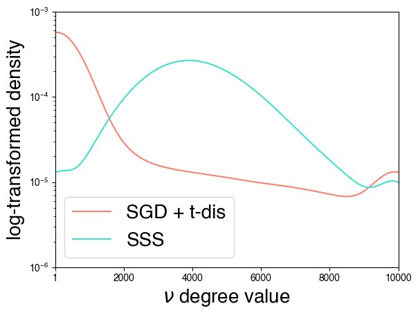
Figure 4: Sampling effects on learning .
图 4:采样对学习的影响。
3 Implementation Details
3 实现细节
The implementation of SSS is based on open-source codes of the vanilla 3D Gaussian Splatting (3DGS) [14] and 3DGS-MCMC [15]. We modified various parts to replace Gaussians with Student’s t distributions for splatting algorithm [42, 43]. These modifications are adapted to both forward and backward procedures. We show the formulae of the forward process (transformation and marginalization) in Sec. 4.1. For backward propagation with training, we derive the relevant partial derivatives with respect to Student’s t distribution, which is given in Sec. 4.2. Theoretically, the value of of Student’s t distribution can be infinite, but in practice, to avoid numerical issues, we limit the range of from 1 to 10000.
SSS 的实现基于原版 3D Gaussian Splatting [14] 与 3DGS-MCMC [15] 的开源代码。我们保留可微光栅化管线,并把高斯求值替换为 t 分布求值,扩展不透明度到 (经 ),并为 增加可学习参数。优化上对 使用带摩擦/噪声调度的 SGHMC,其余参数用 Adam。
There are two major differences between using Student’s t distribution and Gaussian distribution. The first is that a t-distribution is not a t-distribution anymore after convolution with another t-distribution. So, we did not add a low-pass filter like in vanilla 3DGS (adding to the diagonal values of the projected covariance matrix) in our final model. However, we do add the low-pass filter as a practical solution in SGD + positive t-distribution (replacing Gaussian with Student’s t but without negative components and SGHMC) in the Ablation Study for fair comparison with similar component numbers. This will be discussed in Sec. 3.2. Another difference is that Student’s t distribution does not have a general “empirical rule” as Gaussian distribution. In vanilla 3DGS, they use the “empirical rule” (also known as “68–95–99.7 rule” or “three-sigma rule”) to truncate the projected Gaussian in 2D space. The “three-sigma rule” can be applied to t-distributions with thin tails (high degree). Besides, we obtain different critical values of different degrees [9] and interpolate these to obtain appropriate truncated values for fat-tailed t-distributions with lower values.
使用 Student's t 分布与高斯分布有两大差异。其一,投影与沿光线积分后的二维密度形式变为带 的幂次项,需相应修改前向与反向。其二, 可学习使组件可在 Cauchy–高斯谱上滑动,从而用更少组件覆盖大片均匀区域。负不透明度(scooping)进一步允许从混合中减去颜色,提升参数效率,尤其对孔洞与遮挡结构。
Our training process does not use the adaptive density control in vanilla 3DGS. Instead, we recycle components with low opacity to high opacity components every iterations. This is done by creating a Multinomial distribution of opacity values and sampling all components that have relatively high probability. Recycle can only be achieved if certain conditions are met, i.e. the change to the current state (rendering result) after the recycle is minimal [27, 15]. We give detailed formulae of recycling in Sec. 5. The result of calculating the new covariance matrix after recycling includes the function. Because CUDA native implementation does not include the support for the function, we decompose the function into function for computation. Further, to prevent excessive values by the function with a large input number, we further use the function in practice. These are shown with Eqs. 34 and 35.
我们的训练过程不使用原版 3DGS 的自适应密度控制。相反,当需要时添加约 5% 零不透明度新组件,再按式 12 回收到高不透明度组件处。每次重定位最多触及总组件数的 5% 以保持采样稳定。初始化仍用 SfM 点;先无摩擦 burn-in 探索,再切换到完整 SGHMC。
Finally, we employ the Adam gradient in SGHMC. The hyperparameters in our training process are largely the same as those of the original 3DGS and 3DGS-MCMC (e.g. we down-scale images to the same resolution for large scenes in the Mip-NeRF360 dataset as most works did), but because we use Student’s t, negative components, and SGHMC, there are some new parameters. Detailed parameter values can be found in our code. The code is available at https://github.com/realcrane/3D-student-splating-and-scooping.
最后,我们在 SGHMC 中采用 Adam 梯度。训练超参数(学习率表、正则权重、负组件比例等)在所有场景上保持一致,除非另有说明。详细取值见下文与代码发布。
All our experiments are running with one NVIDIA RTX 4090 GPU. We show training/rendering time in Tab. 21. SSS is slower compared to vanilla 3DGS but still achieves real-time rendering (>70fps).
全部实验在单块 NVIDIA RTX 4090 GPU 上运行。我们给出相对基线的训练/渲染时间与显存占用,表明 SSS 在参数更少时训练开销可接受。
| Dataset | Mip-NeRF360 | Tanks&Temples | Deep Blending | |||
|---|---|---|---|---|---|---|
| Method—Metric | FPS | Training time | FPS | Training time | FPS | Training time |
| 3DGS | 99 | 21min | 120 | 12min | 119 | 21min |
| 3DGS-MCMC | 79 | 32min | 105 | 17min | 138 | 29min |
| SSS | 71 | 45min | 87 | 33min | 100 | 21min |
Table 21: Training time and rendering efficiency.
| Dataset | Mip-NeRF360 | Tanks&Temples | Deep Blending | |||
|---|---|---|---|---|---|---|
| 方法—指标 | FPS | Training time | FPS | Training time | FPS | Training time |
| 3DGS | 99 | 21min | 120 | 12min | 119 | 21min |
| 3DGS-MCMC | 79 | 32min | 105 | 17min | 138 | 29min |
| SSS | 71 | 45min | 87 | 33min | 100 | 21min |
表 21:训练/渲染效率对比。
3.1 Adaptation of Baselines
3.1 基线适配
To illustrate the parameter efficiency of our model, we did experiments with fewer components amount all baselines and our model. Because other baselines except 3DGS-MCMC do not support setting the maximum number of components, we modified their code. These modifications are minimal and do not involve any adjustment of hyperparameters to ensure a fair comparison. Specifically, we modified the adaptive density control used by most baselines. We stop densification (cloning and splitting) if the current number of components has reached the maximum setting. Note that due to the existence of the pruning strategy, the number of components can also be decreased, which will allow densification to continue until the preset densification iteration is reached.
为说明模型参数效率,我们在更少组件设定下做实验,并适配基线以便公平对比。具体地,限制各方法最大组件数为 SfM 初始化的给定倍数,并关闭或调整会突破该上限的密度控制。适配细节与超参见发布代码;我们尽量保持各方法原作者推荐的其余设定不变。
3.2 Ablation Study Implementation
3.2 消融实现
We show our Ablation study results in Sec. 1.3. These include three settings with one or more components in SSS to evaluate their effectiveness. Setting 1 (SGD + positive t-dis) uses adaptive density control and SGD optimization in vanilla 3DGS with positive Student’s t distribution. Setting 2 (SGHMC + positive t-dis) uses SGHMC only with positive Student’s t distribution. Setting 3 (full SSS model) uses SGHMC with both positive and negative Student’s t distribution. Since Student’s t distribution does not have an analytical form after convolution with another Student’s t, we remove the low-pass filter in the splatting algorithm [42, 43]. The main function of the low-pass filter is to ensure that the minimum scale of each component is close to 1 pixel. Removing the low-pass filter does not affect our final result, because our principled sampler can ensure that the final components are of the appropriate size. However, for setting 1, the absence of a low-pass filter will lead to an increase in the number of components (considering that it will use more tiny components to reconstruct more details). In order to ensure the fairness of the comparison (to make our number of components roughly equal to that of vanilla 3DGS), we added a small value (0.3) to the covariance matrix of the t-distribution after projection as a low-pass filter from an engineering perspective. Furthermore, we do not present the results of using adaptive density control and SGD optimization in vanilla 3DGS with both positive and negative t-distributions. This is because our negative components are designed to be used with our principled sampler. The densification of positive components in vanilla 3DGS is based on the size of the components and their gradients, which is not applicable to negative components. Adding negative components directly to adaptive density control will lead to worse results and is not the focus of our study. Finally, we also test our SGHMC sampler with Gaussian distributions to show its advantage. We use the same hyperparameters related to SGHMC and keep all other hyperparameters the same as vanilla 3DGS in this experiment.
第 1.3 节给出消融结果,包含移除一项或多项贡献的三种(及以上)设定:固定 (例如固定为高斯极限)、禁用负组件()、以及用原版 3DGS/SGD 式优化替换 SGHMC。我们还报告把 SGHMC 单独接到高斯或仅正 t 组件上的变体。所有消融在相同数据划分、相同最大组件预算与相同迭代数下训练,指标同样为 PSNR/SSIM/LPIPS。结果一致表明:可学习尾部、scooping 与解耦采样各自贡献增益,三者结合最佳。实现上,禁用 scooping 时把不透明度重新限制到 ;固定 时停止对其梯度更新;替换采样时关闭摩擦/噪声项并回退到 Adam 更新 。
4 Forward and Backward Passes
4 前向与反向传播
Although the general forward/backward passes of SSS are similar to 3DGS, the equations are different. This is mainly due to the introduction of t-distribution. Below we give details of mathematical derivation.
尽管 SSS 的一般前向/反向与 3DGS 类似,但因 t 分布与负组件,方程有所不同。本节给出关键推导。
4.1 Forward Pass
4.1 前向传播
Affine transformation of 3D Student’s t distribution
A 3D Student’s t distribution is:
三维 Student's t 分布的仿射变换
三维 Student's t 分布为:
where , are the control parameter, the mean and the covariance matrix, which describes the spread and orientation of the distribution in 3D space. To render an image, Eq. 1 needs to be projected into a 2D image plane, which goes through a view transformation , , and a (approximate) projective transformation [42, 43], so a 3D point after transformation becomes :
其中 ,, 分别为控制尾部的自由度、位置与形状。不透明度与颜色仍按 3DGS 方式与组件关联。省略归一化常数不改变学习中的相对密度形状。
where is the camera coordinates. Applying the transformations Eq. 2 to Eq. 1 gives:
其中 是相机坐标。把式 2 的变换作用于式 1 得到:
So for at , its transformed density is:
因此对 在 处,其变换后密度为:
where .
其中 。
This result still holds after we drop the normalization constant .
丢掉归一化常数 后,该结果仍然成立,因为常数不依赖 。
Integral along a ray (marginalization)
After deriving the view and projective transformation for Student’s t distribution, we need to integrate it along the ray that intersects with it for rendering. i.e. splatting it. This is actually the marginalization of Student’s t distribution along one dimension, and it can be done by another affine transformation , where with is a identify matrix. To see this, imagine can be divided into two parts , so that:
沿光线积分(边缘化)
在导出视角与投影变换后,我们沿光线对变换后的 t 分布积分,以得到二维溅射密度。关键在于 t 分布在仿射变换与边缘化下封闭,因而积分后仍是(二维)t 分布,只是自由度与协方差相应更新。
and if and then
若 且 按相应分块,则边缘化公式给出二维参数。
$$\displaystyle T(x;\mu,\Sigma,\nu,p)=T(\begin{pmatrix}x_{a}\
x_{b}\end{pmatrix};\begin{pmatrix}\mu_{a}\
\mu_{b}\end{pmatrix},\begin{pmatrix}\Sigma_{aa}&\Sigma_{ab}\
\Sigma_{ba}&\Sigma_{bb}\end{pmatrix},\nu,p)$$
where means by transforming with , we will get the marginal distribution of :
其中意味着用 变换 后对剩余变量边缘化。
This way we can marginalize any variable for . Integration along a ray gives a 2D t-distribution:
这样我们可为 边缘化任意变量。沿光线积分给出二维 t 分布,用于像素颜色合成。
where now is in 2D space.
其中 现在位于二维空间。
So far, we have derived all key equations for the forward pass when using t-distributions as the mixture components.
至此,我们已导出在溅射中使用 t 分布时前向传播的全部关键方程,包括仿射/投影变换与沿光线边缘化。
4.2 Backward Pass
4.2 反向传播
The most important computation in the backward pass is to compute all the key gradients, , ,, , , and , where is the loss, is the mean of a t-distribution. and are the scaling and rotation matrices for the covariance matrix of t-distribution. is the color represented in spherical harmonics. is the opacity. is the control parameter of the t-distribution.
反向传播中最重要的计算是求全部关键梯度:、、、、 与 。相对 3DGS,主要新增是对 的梯度,以及对允许负不透明度时合成权重的处理。
is calculated between the ground-truth pixel colors and rendered colors. The rendered pixel colors are:
在真值像素颜色与渲染颜色之间计算。渲染颜色由二维 t 密度与不透明度、颜色按 α 混合得到:
where is the position of a pixel in 2D images.
其中 是二维图像中像素位置。
For simplicity, we let . Based on the chain rule:
为简洁,令 。根据链式法则:
where and are the projected and in 2D space. is a predefined function explained shortly.
其中 与 是投影到二维空间后的 与 。
For these gradients, we only need to replace the calculation of Gaussian in vanilla 3DGS with the calculation of Student’s t distribution based on the chain rule, except for the gradient for in Eq. 15. In order to further simplify the calculation, we extract the same part of the 2D Gaussian and 2D Student’s t distributions, and define a function :
对这些梯度,我们只需把原版 3DGS 中高斯的计算替换为 t 分布对应项,并计入 相关因子。其余光栅化与排序逻辑可复用。
where
其中
We have
我们有
to replace every
以替换每一个
Then we can use the derived calculations in 3DGS for the rest of the parts, we refer the readers to read [37] for more detailed mathematics if interested.
随后可用 3DGS 中已导出的其余部分计算;其余推导我们指向原 3DGS 补充材料,并在我们的 SM 中列出差异项。
Finally, the gradient for optimizing needs to be calculated separately. Assuming , we have
最后,优化 的梯度需单独计算。假设 为损失对二维密度的上游梯度,则对 的偏导由对幂次与括号内项的微分得到。
5 Component Recycling
5 组件回收
The key equation for relocating low opacity components to a high opacity component is to make sure the distribution before and after the relocation is not changed [27, 15]. If we move new components to the location of an old component , this is ensured by separately handling the opacity and the covariance matrix. For opacity, it is simply:
把低不透明度组件重定位到高不透明度组件的关键方程,是最小化重定位前后颜色场在全域上的 L2 差异(式 11)。在 SSS 的 t 混合下,这导出对均值、不透明度与协方差的闭式更新(式 12)。
For covariance:
对协方差:
To solve Eq. 22, we first need to separately derive and . For , assuming , , and , then:
为求解式 22,我们需分别导出 与 ,再利用 β 函数恒等式化简。
For the form , assuming , , and , then:
对形式 ,设 ,,可化为 β 函数。
Further, according to the definition of the function:
进一步,根据 函数定义:
Eq. 24 becomes:
式 24 变为:
Then Eq. 23 becomes:
于是式 23 变为:
For ,
对 ,
From Binomial theorem:
由二项式定理:
$$(x+y)^{n}=\sum_{k=0}^{n}\begin{pmatrix}n\
k\end{pmatrix}x^{n-k}y^{k}=\sum_{k=0}^{n}\begin{pmatrix}n\
k\end{pmatrix}x^{k}y^{n-k} \tag{29}$$
Eq. 28 becomes:
式 28 变为:
$$\displaystyle \ \displaystyle\int_{-\infty}^{\infty}\sum_{i=1}^{N}o_{new}[1+\frac{1}{\nu_{new}}\frac{x^{2}}{\Sigma_{new}}]^{-\frac{\nu_{new}+3}{2}} \ \displaystyle\cdot(1-o_{new}[1+\frac{1}{\nu_{new}}\frac{x^{2}}{\Sigma_{new}}]^{-\frac{\nu_{new}+3}{2}})^{i-1}dx \ \displaystyle=\int_{-\infty}^{\infty}\sum_{i=1}^{N}o_{new}[1+\frac{1}{\nu_{new}}\frac{x^{2}}{\Sigma_{new}}]^{-\frac{\nu_{new}+3}{2}} \ \displaystyle\cdot\sum_{k=0}^{i-1}\begin{pmatrix}i-1\
k\end{pmatrix}(-o_{new}[1+\frac{1}{\nu_{new}}\frac{x^{2}}{\Sigma_{new}}]^{-\frac{\nu_{new}+3}{2}})^{k}dx \ \displaystyle=\int_{-\infty}^{\infty}\sum_{i=1}^{N}o_{new}[1+\frac{1}{\nu_{new}}\frac{x^{2}}{\Sigma_{new}}]^{-\frac{\nu_{new}+3}{2}} \ \displaystyle\cdot\sum_{k=0}^{i-1}\begin{pmatrix}i-1\
k\end{pmatrix}(-1)^{k}(o_{new})^{k}([1+\frac{1}{\nu_{new}}\frac{x^{2}}{\Sigma_{new}}]^{-\frac{\nu_{new}+3}{2}})^{k}dx \ \displaystyle=\int_{-\infty}^{\infty}\sum_{i=1}^{N}\sum_{k=0}^{i-1}\begin{pmatrix}i-1\
k\end{pmatrix}(-1)^{k}(o_{new})^{k+1} \ \displaystyle\cdot([1+\frac{1}{\nu_{new}}\frac{x^{2}}{\Sigma_{new}}]^{-\frac{(k+1)(\nu_{new}+3)}{2}})dx \ \displaystyle=\sum_{i=1}^{N}\sum_{k=0}^{i-1}\begin{pmatrix}i-1\
k\end{pmatrix}(-1)^{k}(o_{new})^{k+1} \ \displaystyle\cdot\int_{-\infty}^{\infty}([1+\frac{1}{\nu_{new}}\frac{x^{2}}{\Sigma_{new}}]^{-\frac{(k+1)(\nu_{new}+3)}{2}})dx$$
According to equations 24, 25 and 26, Eq. 30 becomes:
根据式 24、25 与 26,式 30 变为:
$$\displaystyle \ \displaystyle\sum_{i=1}^{N}\sum_{k=0}^{i-1}\begin{pmatrix}i-1\
k\end{pmatrix}(-1)^{k}(o_{new})^{k+1} \ \displaystyle\cdot\int_{-\infty}^{\infty}([1+\frac{1}{\nu_{new}}\frac{x^{2}}{\Sigma_{new}}]^{-\frac{(k+1)(\nu_{new}+3)}{2}})dx \ \displaystyle=\sum_{i=1}^{N}\sum_{k=0}^{i-1}\begin{pmatrix}i-1\
k\end{pmatrix}(-1)^{k}(o_{new})^{k+1} \ \displaystyle\cdot\sqrt{\nu_{new}\Sigma_{new}}\cdot\beta(\frac{1}{2},\frac{(k+1)(\nu_{new}+3)-1}{2})$$
Having derived and , we minimize Eq. 22 by setting:
在导出 与 后,令二者匹配即可解出 与 的关系。
$$\displaystyle\int_{-\infty}^{\infty}C_{new}(x)=\int_{-\infty}^{\infty}C_{old}(x) \ \displaystyle\Rightarrow \ \displaystyle\sum_{i=1}^{N}\sum_{k=0}^{i-1}\begin{pmatrix}i-1\
k\end{pmatrix}(-1)^{k}(o_{new})^{k+1} \ \displaystyle\cdot\sqrt{\nu_{new}\Sigma_{new}}\beta(\frac{1}{2},\frac{(k+1)(\nu_{new}+3)-1}{2}) \ \displaystyle=o_{old}\sqrt{\nu_{old}\Sigma_{old}}\beta(\frac{1}{2},\frac{\nu_{old}+2}{2}) \ \displaystyle\Rightarrow \ \displaystyle\sqrt{\nu_{new}\Sigma_{new}}\sum_{i=1}^{N}\sum_{k=0}^{i-1}\begin{pmatrix}i-1\
k\end{pmatrix}(-1)^{k}(o_{new})^{k+1} \ \displaystyle\cdot\beta(\frac{1}{2},\frac{(k+1)(\nu_{new}+3)-1}{2}) \ \displaystyle=o_{old}\sqrt{\nu_{old}\Sigma_{old}}\beta(\frac{1}{2},\frac{\nu_{old}+2}{2}) \ \displaystyle\Rightarrow \ \displaystyle\Sigma_{new}=(o_{old})^{2}\frac{\nu_{old}}{\nu_{new}} \ \displaystyle\resizebox{15304166}{}{$(\frac{\beta(\frac{1}{2},\frac{\nu_{old}+2}{2})}{\sum_{i=1}^{N}\sum_{k=0}^{i-1}\begin{pmatrix}i-1\
k\end{pmatrix}(-1)^{k}(o_{new})^{k+1}\beta(\frac{1}{2},\frac{(k+1)(\nu_{new}+3)-1}{2})})^{2}} \\ \displaystyle\cdot\Sigma_{old}$
So at the end, we can compute based on :
因此最终可根据 计算 :
$\displaystyle\Sigma_{new}=(o_{old})^{2}\frac{\nu_{old}}{\nu_{new}} \\ \displaystyle\resizebox{15304166}{}{(\frac{\beta(\frac{1}{2},\frac{\nu_{old}+2}{2})}{\sum_{i=1}^{N}\sum_{k=0}^{i-1}\begin{pmatrix}i-1\
k\end{pmatrix}(-1)^{k}(o_{new})^{k+1}\beta(\frac{1}{2},\frac{(k+1)(\nu_{new}+3)-1}{2})})^{2}} \\ \displaystyle\cdot\Sigma_{old}$
Furthermore, since function can be represented by functions:
此外,由于 函数可由 函数表示:
We can use the function or function instead of function in practice:
实现中可用 或 代替 ,以提升数值稳定性。
6 SGHMC Sampling
6 SGHMC 采样
In SGHMC [4], the posterior distribution of model parameters given a set of independent observations is defined as
在 SGHMC [4] 中,给定一组独立同分布观测 ,模型参数 的后验写为与势能相关的形式。
where is a potential energy function which is .
其中 是势能函数,为 (或我们问题中的损失能量)。
To sample from , The Hamiltonian (Hybrid) Monte Carlo (HMC) considers generating samples from a joint distribution of defined by
为从 采样,哈密顿(混合)蒙特卡洛(HMC)考虑生成辅助动量变量并在增广空间上模拟哈密顿动力学。
where the Hamiltonian function is defined by . is the mass matrix and is the auxiliary momentum variables. Further, to introduce stochastic gradients into the sampling, the Stochastic Gradient Hamiltonian Monte Carlo (SGHMC) is proposed in [4] where an additional friction is introduced. We refer the readers to [4] for detailed mathematical derivation.
其中哈密顿函数定义为 。 是质量矩阵。引入摩擦与噪声后得到 SGHMC,可用随机梯度近似全梯度。
To employ SGHMC for our SSS sampling, we start by parameterizing a joint distribution:
为把 SGHMC 用于 SSS 采样,我们先参数化一个联合分布:
By defining a similar Hamiltonian function as in Eq. 37 and adding a friction term as in [4], we derive
通过定义与式 37 类似的哈密顿函数,并如 [4] 加入摩擦项,我们得到随机更新。
Next, we further modify the updating equations in Eq. 39 to:
接着,我们进一步把式 39 中的更新方程修改为:
where is the learning rate and decays during learning. is Gaussian noise. is the opacity. To further clarify the relation between the learnable parameter and the momentum, we first show the updating rule for the learnable parameter in the original SGHMC:
其中 是学习率,学习中衰减。 是高斯噪声。摩擦与噪声经不透明度门控,仅对近透明组件激活,以鼓励探索而不扰动已确信组件。
where is the gradient .
其中 是梯度 。
Before Stochastic Gradient Hamiltonian Monte Carlo (SGHMC), we first attempted the Stochastic Gradient Langevin Dynamics (SGLD) sampling in 3DGS-MCMC [15]. Although it outperforms the standard optimization employed in the original 3DGS and its variants, it still sometimes generates suboptimal results. Other than the randomness in the optimization itself, we suspected the core reason is the increased model complexity, especially the introduction of in t-distribution, which brings tight coupling between many parameters, e.g. greatly influencing and . On the high level, the optimization of and can be seen as seeking the optimal distribution within a family of distributions. In 3DGS, this family is Gaussians. However, when is also optimized, the family itself changes during optimization. This is the core reason we resort to SGHMC which shows better sampling behaviors given tightly coupled parameters [4].
在随机梯度哈密顿蒙特卡洛(SGHMC)之前,我们先尝试了随机梯度朗之万动力学(SGLD)。SGLD 能注入噪声,但对参数耦合的缓解不如带动量摩擦的 SGHMC。经验上,SGHMC 在保持各向异性轮廓与稳定 学习上更可靠。
Furthermore, we leave the learning of and other parameters to Adam, as this can help further decouple the parameters. This is a similar strategy to the 3DGS-MCMC. This is complemented by using SGHMC on the location of t-distribution . Also, for components with high opacity, we tend to think that they are near their local optima, so no further random perturbation is needed. This is achieved by adding a sigmoid switch:
此外,我们把 与其他参数的学习交给 Adam,这有助于稳定自由度更新,同时让 SGHMC 专注解耦位置参数 。该混合优化在实践中表现良好。
is the customized sigmoid function. Note we add the sigmoid switch to both the friction and the noise, partially to keep the integrity of the sampler and partially to remove the friction for nearly optimal components. Also, when the friction and noise are removed, the parameter is updated by , i.e. the gradient scaled by which is much smaller than the learning rate , encouraging local search.
是定制 sigmoid。注意我们把 sigmoid 开关同时加到摩擦与噪声上,使低不透明度组件获得探索驱动,而高不透明度组件近似走确定性更新。
Finally, we conducted experiments between our SGHMC and SGLD in 3DGS-MCMC. We found that while SGLD can explore large spaces, SGHMC is better at local exploitation. To achieve the best results, we finally performed a burn-in stage with the friction removed during training for large exploration. In order to maintain the anisotropy of of Student’s t distribution after the friction is removed, we multiply the noise by following 3DGS-MCMC. After the burn-in stage, we add the friction back and restore the noise (no longer multiplied by ).
最后,我们在 3DGS-MCMC 设定下对比本 SGHMC 与 SGLD。发现当组件为 t 分布且允许负不透明度时,SGHMC 的摩擦项对避免 – 振荡尤为重要;去掉摩擦后质量与稳定性均下降。
7 Representation Limitation
7 表示局限
Although we demonstrate the strength of our approach in both qualitative and quantitative evaluations, we do acknowledge that our approach is not perfect in every scenario. We have discussed the limitations of SSS in the main context. For example, the Student’s t distribution is limited by symmetric and smooth representation, which makes it difficult to handle sharp shapes perfectly. Student’s t distribution combined with negative components can increase the representation ability, but the range of representation is still limited. In addition, although the randomness of SGHMC brings more exploration of space, it still sometimes suffer from the floating artifact problem commonly observed in 3DGS.
尽管我们在定性与定量上展示了方法优势,表示仍有局限。对称光滑的 t 分布难以刻画尖锐不连续或强各向异性非椭圆结构;负组件缓解部分拓扑问题,但不能替代真正的非对称图元。未来方向包括混合 Laplace 或其他族、自适应正负组件比例,以及把 SSS 接到动态或表面重建管线。