Stochastic Taylor Derivative Estimator: Efficient amortization for arbitrary differential operators
Stochastic Taylor Derivative Estimator: Efficient amortization for arbitrary differential operators
随机泰勒导数估计器:任意微分算子的高效摊销
Zekun Shi Affiliation: National University of Singapore Affiliation: Sea AI Lab Email: shizk@sea.com , Zheyuan Hu Affiliation: National University of Singapore Email: e0792494@u.nus.edu , Min Lin Affiliation: Sea AI Lab Email: linmin@sea.com , Kenji Kawaguchi Affiliation: National University of Singapore Email: kenji@nus.edu.sg
Abstract
摘要
Optimizing neural networks with loss that contain high-dimensional and high-order differential operators is expensive to evaluate with back-propagation due to scaling of the derivative tensor size and the scaling in the computation graph, where is the dimension of the domain, is the number of ops in the forward computation graph, and is the derivative order. In previous works, the polynomial scaling in was addressed by amortizing the computation over the optimization process via randomization. Separately, the exponential scaling in for univariate functions () was addressed with high-order auto-differentiation (AD). In this work, we show how to efficiently perform arbitrary contraction of the derivative tensor of arbitrary order for multivariate functions, by properly constructing the input tangents to univariate high-order AD, which can be used to efficiently randomize any differential operator. When applied to Physics-Informed Neural Networks (PINNs), our method provides >1000 speed-up and >30 memory reduction over randomization with first-order AD, and we can now solve 1-million-dimensional PDEs in 8 minutes on a single NVIDIA A100 GPU[^1]. This work opens the possibility of using high-order differential operators in large-scale problems.
若损失函数含高维、高阶微分算子,用反向传播求值代价很高:导数张量规模按 增长,计算图规模按 增长,其中 是定义域维数, 是前向计算图中的运算数, 是导数阶数。先前工作通过随机化把计算摊销到优化过程中,缓解了 上的多项式增长;对单变量函数()则用高阶自动微分(AD)应对 上的指数增长。本文说明:只要恰当构造一元高阶 AD 的输入切向量,就能对多元函数任意阶导数张量做任意收缩,从而高效随机化任意微分算子。用于物理信息神经网络(PINN)时,相对一阶 AD 的随机化,本方法加速超过 1000 倍、显存降低超过 30 倍,并可在单块 NVIDIA A100 上于 8 分钟内求解百万维 PDE[^1]。这为在大规模问题中使用高阶微分算子打开了可能。
1 Introduction
1 引言
In many problems, especially in Physics-informed machine learning [19, 33], one needs to solve optimization problems where the loss contains differential operators:
在许多问题中,尤其是物理信息机器学习 [19, 33],需要求解损失里含微分算子的优化问题:
In this above, , is a multi-index, is some neural network parameterized by , and is some cost function. When either the differentiation order or the dimensionality is high, the objective function above is expensive to evaluate with back-propagation (backward mode AD) in both memory and computation: the size of the derivative tensor has scaling , and the size of the computation graph has scaling where is the number of ops in the forward computation graph.
上式中 , 是多重指标, 是由 参数化的神经网络, 是代价函数。当微分阶数 或维数 很高时,用反向传播(反向模式 AD)求目标函数在显存与计算上都很贵:导数张量规模为 ,计算图规模为 , 是前向图中的运算数。
There have been several efforts to tackle this curse of dimensionality. One line of work uses randomization to amortize the cost of computing differential operators with AD over the optimization process so that the in the above scaling becomes a constant for the case of . Stochastic Dimension Gradient Descent (SDGD) [13] randomizes over the input dimensions where in each iteration, the partial derivatives are only calculated for a minibatch of sampled dimensions with back-propagation. In [12, 21, 15], the classical technique of Hutchinson Trace Estimator (HTE) [16] is used to estimate the trace of Hessian or Jacobian to inputs. Others choose to bypass AD completely to reduce the complexity of computation. In [31], the finite difference method is used for estimating the Hessian trace. Randomized smoothing [11, 14] uses the expectation over Gaussian random variable as ansatz, so that its derivatives can be expressed as another expectation Gaussian random variable via Stein’s identity [39]. However, compared to AD, the accuracy of these methods is highly dependent on the choice of discretization.
已有若干工作试图打破维数灾难。一类做法用随机化,把用 AD 算微分算子的代价摊到优化过程中,使 时上述缩放里的 变成常数。随机维梯度下降(SDGD)[13] 对输入维做随机采样,每轮只用反向传播算一小批维上的偏导。[12, 21, 15] 用经典 Hutchinson 迹估计(HTE)[16] 估计 Hessian 或对输入的 Jacobian 的迹。另一些工作干脆绕过 AD 以降复杂度:[31] 用有限差分估 Hessian 迹;随机平滑 [11, 14] 以高斯期望作 ansatz,再经 Stein 恒等式 [39] 把导数写成另一高斯期望。但相对 AD,这些方法的精度高度依赖离散化选择。
In this work, we address the scaling issue in both and for the optimization problem in Eq. 1 at the same time, by proposing an amortization scheme that can be efficiently evaluated via high-order AD, which we call Stochastic Taylor Derivative Estimator (STDE). Our main contributions are:
本文同时应对式 (1) 中 与 两边的缩放问题:提出可经高阶 AD 高效求值的摊销方案,称为随机泰勒导数估计器(STDE)。主要贡献如下:
- • We demonstrate how Taylor mode AD [6], a high-order AD method, can be used to amortize the optimization problem in Eq. 1. Specifically, we show that, with properly constructed input tangents, the univariate Taylor mode can be used to contract multivariate functions’ derivative tensor of arbitrary order;
- • We provide a comprehensive procedure for randomizing arbitrary differential operators with STDE, while previous works mainly focus on the Laplacian operator, and we provide abundant examples of STDE constructed for operators in common PDEs;
- • STDE encompass and generalizes previous methods like SDGD [13] and HTE [16, 12]. We also prove that HTE-type estimator cannot be generalized beyond fourth order differential operator;
- • We determine the efficacy of STDE experimentally. When applied to PINN, our method provides a significant speed-up compared to the baseline method SDGD [13] and the backward-free method like random smoothing [11]. Due to STDE’s low memory requirements and reduced computation complexity, PINNs with STDE can solve 1-million-dimensional PDEs on a single NVIDIA A100 40GB GPU within 8 minutes, which shows that PINNs have the potential to solve complex real-world problems that can be modeled as high-dimensional PDEs. We also provide a detailed ablation study on the source of performance gain of our method.
- • 说明如何用高阶 AD 方法——Taylor 模式 AD [6]——摊销式 (1) 的优化;具体地,在恰当构造输入切向量后,一元 Taylor 模式可用来收缩多元函数任意阶导数张量;
- • 给出用 STDE 随机化任意微分算子的完整流程(先前工作多集中在 Laplace 算子),并给出常见 PDE 算子上的大量 STDE 构造例子;
- • STDE 涵盖并推广 SDGD [13] 与 HTE [16, 12];我们还证明 HTE 型估计器无法推广到四阶以上微分算子;
- • 用实验验证 STDE 的效力。用于 PINN 时,相对基线 SDGD [13] 以及无反向的随机平滑 [11] 有显著加速;因显存需求低、计算复杂度降,带 STDE 的 PINN 可在单块 NVIDIA A100 40GB 上 8 分钟内求解百万维 PDE,表明 PINN 有望处理可建模为高维 PDE 的复杂现实问题。我们也对性能增益来源做了细消融。
2 Related works
2 相关工作
High-order and forward mode AD
The idea of generalizing forward mode AD to high-order derivatives has existed in the AD community for a long time [5, 18, 40, 22]. However, accessible implementation for machine learning was not available until the recent implementation in JAX [6, 7], which implemented the Taylor mode AD for accelerating ODE solver. There are also efforts in creating the forward rule for a specific operator like the Laplacian [24, 23]. Randomization over the linearized part of the AD computation graph was considered in [30]. Forward mode AD can also be used to compute neural network parameter gradient as shown in [2].
高阶与前向模式 AD
把前向模式 AD 推广到高阶导数,在 AD 社区早已有之 [5, 18, 40, 22]。但面向机器学习、可直接用的实现直到近期 JAX [6, 7] 才出现——其为加速 ODE 求解实现了 Taylor 模式 AD。也有工作为 Laplace 等特定算子写前向规则 [24, 23]。[30] 考虑对 AD 计算图线性化部分做随机化。前向模式 AD 也可用来算神经网络参数梯度,见 [2]。
Randomized Gradient Estimation
Randomization [28, 29, 8] is a common technique for tackling the curse of dimensionality for numerical linear algebra computation, which can be applied naturally in amortized optimization [1]. Hutchinson trace estimator [16] is a well-known technique, which has been applied to diffusion model [37] and PINNs [12]. Another case that requires gradient estimation is when the analytical form of the target function is not available (black box), which means AD cannot be applied. The method of zeroth-order optimization [25] can be used in this case, as it only requires evaluating the function at arbitrary input. It is also useful when the function is very complicated like in the case of a large language model [27].
随机梯度估计
随机化 [28, 29, 8] 是数值线性代数里对付维数灾难的常用手段,自然可用于摊销优化 [1]。Hutchinson 迹估计 [16] 广为人知,已用于扩散模型 [37] 与 PINN [12]。另一类需要梯度估计的情形是目标函数解析式不可得(黑盒),因而无法用 AD;此时可用零阶优化 [25],只要求在任意输入上求函数值。对大语言模型这类极复杂函数也有用 [27]。
3 Preliminaries and discussions
3 预备知识与讨论
3.1 First-order auto-differentiation (AD)
3.1 一阶自动微分(AD)
AD is a technique for evaluating the gradient of composition of known analytical functions commonly called primitives. In an AD framework, a neural network is constructed as the composition of primitives that are parameterized by some parameters . In this section, we will consider the neural networks with linear computation graphs like , but the results generalize to arbitrary directed acyclic graphs (DAGs). We will assume that all hidden dimensions are . See Appendix B for more details on first-order AD.
AD 用于求由已知解析函数(常称原语)复合而成的函数的梯度。在 AD 框架中,神经网络 由带参数 的原语 复合而成。本节先考虑线性计算图 ,结论可推广到任意有向无环图(DAG)。假设所有隐层维数为 。一阶 AD 更多细节见附录 B。
Forward mode AD
Each primitives is linearized as the Fréchet (directional) derivative , which computes the Jacobian-vector-product (JVP): , where is referred to as the primal and the tangent. form a linearized computation graph (third row in Fig. 3), that computes the JVP of the composition :
前向模式 AD
每个原语 被线性化为 Fréchet(方向)导数 ,计算 Jacobian–向量积(JVP):,其中 称主值, 称切向量。 构成线性化计算图(图 3 第三行),用于计算复合的 JVP :
By setting the tangent to one of the standard basis of , JVP computes one column of the Jacobian , so the full Jacobian can be computed with JVPs. Each JVP call requires memory as only the current activation and tangent are needed to carry out the computation, and the computation complexity is usually in the same order as the forward computation graph. In the case of MLP, both the forward and the linearized graph have a complexity of .
把切向量 设为 的某个标准基向量时,JVP 给出 Jacobian 的一列,故完整 Jacobian 需 次 JVP。每次 JVP 只需 显存——只需当前激活 与切向量 ;计算复杂度通常与前向图同阶。对 MLP,前向图与线性化图复杂度均为 。
Backward mode AD
Each primitives is linearized as the adjoint of the Fréchet derivative instead, which computes the vector-Jacobian-product (VJP): where is the cotangent. The linearized computation graph now runs in the reverse order:
反向模式 AD
此时每个原语 线性化为 Fréchet 导数的伴随 ,计算向量–Jacobian 积(VJP):, 为余切。线性化计算图按相反顺序运行:
which is also clear from Fig. 3. Furthermore, due to this reversion, we first need to do a forward pass to obtain the evaluation trace before we can invoke the VJPs , which apparent as shown in Eq. 3. Hence the number of sequential computations is twice as much compared to forward mode. The memory requirement becomes as we need to store the entire evaluation trace. Similar to JVP, VJP computes one row of at a time, so the full Jacobian can be computed using VJPs. When optimizing scalar cost functions of the network parameters , backward mode efficiently trades off memory with computation complexity as and only VJP is needed to get the full Jacobian. Furthermore, all parameter can use the same cotangent , whereas with forward mode, separate tangent for each parameter is needed.
图 3 也清楚显示这一点。由于顺序反转,须先前向得到求值轨迹 ,才能调用 VJP ,见式 (3)。因此串行计算次数约为前向模式的两倍。显存变为 ,因需存整条求值轨迹。与 JVP 类似,VJP 每次给出 的一行,完整 Jacobian 需 次 VJP。优化对参数 的标量代价 时,反向模式在显存与计算间更划算:,一次 VJP 即得完整 Jacobian;且所有 可共用同一余切 ,而前向模式则需为每个 单独准备切向量。
3.2 Inefficiency of the first-order AD for high-order derivative on inputs
3.2 一阶 AD 对输入高阶导数的低效
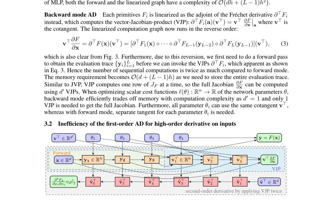
Figure 1: The computation graph of computing second order gradient by repeated application of backward mode AD, for a function with primitives (), which computes the Hessian-vector-product. Red nodes represent the cotangent nodes in the second backward pass. With each repeated application of VJP the length of sequential computation doubles.
图 1:对含 4 个原语()的函数 ,反复用反向模式 AD 求二阶梯度(即 Hessian–向量积)的计算图。红节点表示第二次反向中的余切。每多做一次 VJP,串行计算长度翻倍。
High-order input derivatives for scalar can be implemented as repeated applications of first-order AD, but this approach will exhibit fundamental inefficiency that cannot be remedied by randomization.
标量 对输入的高阶导数 可通过反复套用一阶 AD 实现,但这种方式有根本性低效,随机化也无法消除。
Repeating backward mode AD
With each repeated application of backward mode AD, the new evaluation trace will include the cotangents from the previous application of backward AD, so the length of sequential computation doubles. Furthermore, the size of the cotangent also grows by times. Therefore applying backward mode AD has additional memory cost of and additional computation cost of , which is clear from Fig. 1. In general, with repeated applications of backward mode AD will incur memory cost and computation cost. And calls are needed to evaluate the entire derivative tensor. So both memory and compute scale exponentially in derivative order
反复反向模式 AD
每多做一次反向模式 AD,新的求值轨迹会并入上一次反向的余切,串行计算长度翻倍;余切规模也按 倍增长。因而每次额外反向带来 显存与 计算,见图 1。一般地, 次反复反向的显存为 ,计算为 ;完整导数张量还需 次调用。故显存与计算都对导数阶数 指数增长。
Repeating forward mode AD
Consider . The input tangent dimension is on the first application of forward mode AD, but on the second application, it will become since we are now computing the forward mode AD for . So the size of the input tangent with repeated application is , so it grows exponentially. This is also inefficient.
反复前向模式 AD
考虑 。第一次前向时输入切向量维数为 ;第二次则变成 ,因为此时是对 做前向。 次反复后输入切向量规模为 ,同样指数增长,同样低效。
Mixed mode AD schemes are also likely inefficient
See more detail in Appendix C.
混合模式 AD 方案多半也不高效
详见附录 C。
3.3 Stochastic Dimension Gradient Descent
3.3 随机维梯度下降
SDGD [13] amortizes high-dimensional differential operators by computing only a minibatch of derivatives in each iteration. It replaces a differential operator with a randomly sampled subset of additive terms, where each term only depends on a few input dimensions
SDGD [13] 通过每轮只算一小批导数,摊销高维微分算子。它把微分算子 换成随机采样的若干加性项,每项只依赖少数输入维
where denotes the SDGD operator that approximates the true operator , is the sampled index set, and is the batch size. For example, in -dimensional Poisson equation, , , and the additive terms are .
其中 是逼近真算子 的 SDGD 算子, 是采样指标集, 是批大小。例如 维 Poisson 方程中 ,,加性项为 。
are cheaper to compute than due to reduced dimensionality: for each sampled index, by treating all other input as constant we get a function with scalar input and output. For a given index set , the memory requirements are reduced from to , and the computation complexity reduces to . This reduction is significant when as in the experimental setting of SDGD [13], but the exponential scaling in persists.
因维数降低, 比 更便宜:对每个采样指标,把其余输入当常数,得到标量入、标量出函数。给定 ,显存从 降到 ,计算降到 。在 SDGD [13] 实验设定 时这一降幅显著,但 上的指数缩放仍在。
3.4 Univariate Taylor mode AD
3.4 一元 Taylor 模式 AD
One way to define high-order AD is by determining how the high-order Taylor expansion of a univariate function changes when mapped by primitives. Firstly, the Fréchet derivative can be rewritten to operate on a space curve that passes through the primal , i.e. , and has tangent :
定义高阶 AD 的一种方式是:看一元函数的高阶 Taylor 展开在经原语映射后如何变化。首先,Fréchet 导数 可改写为作用在穿过主值 的空间曲线 上,即 ,且切向量 :
This shows that the (JVP) is the same as the univariate chain rule. The tuple can be thought of as the first-order expansion of which lives in the tangent bundle of . Treating as the smooth map between manifolds, we can define the pushforward which pushes the first order expansion of (i.e. ) forward to the first order expansion of (i.e. ):
这说明 (JVP)与一元链式法则相同。元组 可视为 的一阶展开,落在 的切丛上。把 当作流形间光滑映射,可定义前推 ,把 的一阶展开 前推到 的一阶展开 :
Naturally, to extend this to higher orders, one can consider the th order expansion of the input curve , which is equivalent to the tuple known as the -jet of where is called the th order tangent of . lives in the th order tangent bundle of , and we can define the th-order pushforward :
自然地,推广到更高阶可考虑输入曲线 的 阶展开,即元组 ,称为 的 -jet,其中 是 的 阶切向量。 落在 的 阶切丛上,可定义 阶前推 :
which pushes the th order expansion of (i.e. ) forward to the th order expansion of (i.e. ). is the -th order Fréchet derivative, whose analytical formula is given by the high-order univariate chain rule known as the Faa di Bruno’s formula (Eq. 43).
它把 的 阶展开 前推到 的 阶展开 。 是 阶 Fréchet 导数,其解析式由一元高阶链式法则——Faa di Bruno 公式(式 43)——给出。
Since contains all information needed to evaluate for any , the map is well-defined. defines a high-order AD: we can compute of arbitrary composition from the th-order pushforward of the primitives , since is an homomorphism of the group :
因 含计算任意 的 所需全部信息, 良定义。 定义了高阶 AD:任意复合 的 可由原语的 阶前推 复合得到,因为 是群 的同态:
This approach of composing of primitives is also known as the Taylor mode AD. For more details on Taylor mode AD, see Appendix D.
这种把原语的 复合起来的做法即 Taylor 模式 AD。更多细节见附录 D。
4 Method
4 方法
From the previous discussion, it is clear that the exponential scaling in for the problem described in Eq. 1 cannot be mitigated by amortization alone. Although high-order AD methods like Taylor mode AD [6] can address this scaling issue, it is only defined for univariate functions. In this section, we describe a method that addresses the scaling issue in and simultaneously when amortizing Eq. 1 by seeing univariate Taylor mode AD as contractions of multivariate derivative tensor.
由前文可见,仅靠摊销无法缓解式 (1) 中 上的指数缩放。Taylor 模式 AD [6] 等高阶 AD 可应对该缩放,但只对一元函数定义。本节把一元 Taylor 模式 AD 视为多元导数张量的收缩,从而在摊销式 (1) 时同时解决 与 的缩放。
4.1 Univariate Taylor mode AD as contractions of multivariate derivative tensor
4.1 一元 Taylor 模式 AD 作为多元导数张量的收缩
projects the Jacobian of to with a 1-jet . Similarly, contracts a set of derivative tensors to with a -jet . We can expand with Eq. 43 to see the form of the contractions. For example, is JVP, and contains a quadratic form of the Hessian :
用 1-jet 把 的 Jacobian 投影到 ;同理, 用 -jet 把一组导数张量收缩到 。用式 43 展开 可看出收缩形式。例如 即 JVP, 含 Hessian 的二次型:
From Eq. 43, one can always find a with large enough such that there exists with where , by setting some tangents to the zero vector. That is, arbitrary derivative tensor contraction is contained within a Fréchet derivative of high-order, which can be efficiently evaluated through Taylor mode AD.
由式 43,总能找到足够大的 的 ,使存在 满足(),只需把部分切向量 置零。亦即:任意导数张量收缩都含于某个高阶 Fréchet 导数中,可用 Taylor 模式 AD 高效求值。
How large should be depends on how off-diagonal the operator is. If the operator is diagonal (i.e. contains no mixed partial derivatives), is enough. If the operator is maximally non-diagonal, i.e. it is a partial derivative where all dimensions to be differentiated are distinct, then the minimum needed is . For more details, please refer to Appendix F where a general procedure for determining the jet structure is discussed.
需多大取决于算子有多「非对角」。若算子对角(无混合偏导), 即可;若最大程度非对角——对两两不同的维求偏导——则最小 为 。细节与确定 jet 结构的一般流程见附录 F。
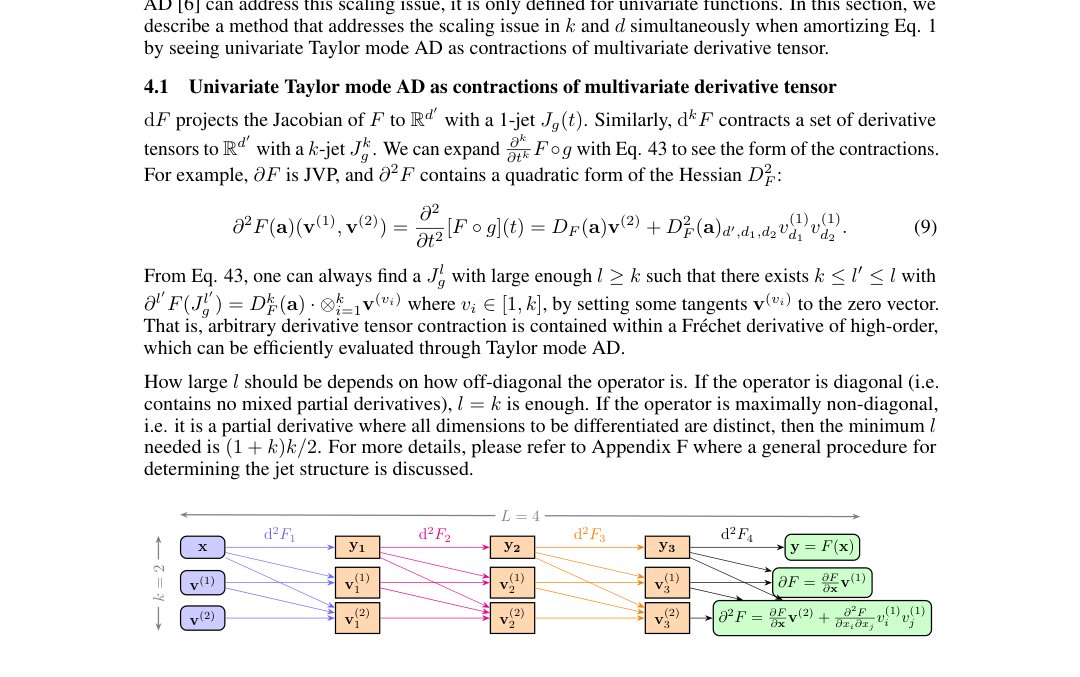
Figure 2: The computation graph of for with primitives. Parameters are omitted. The first column from the left represents the input 2-jet , and pushes it forward to the 2-jet which is the subsequent column. Each row can be computed in parallel, and no evaluate trace needs to be cached.
图 2:含 4 个原语的 上 的计算图。参数 省略。最左列是输入 2-jet , 将其前推为下一列的 2-jet 。各行可并行计算,且无需缓存求值轨迹。
4.2 Estimating arbitrary differential operator by pushing forward random jets
4.2 通过前推随机 jet 估计任意微分算子
Next, we show how to use the above facts to construct a stochastic estimator derivative operator. Differential operators can be evaluated through derivative tensor contraction. The action of the derivative on function can be identified with the derivative tensor slice . Differential operator can be written as a linear combination of derivatives: , where is the set of tensor indices representing terms included in the operator . For simplicity we only consider th order differential operator, i.e. for all . For scalar , we can identify a th order differential operator with the following tensor dot product
下面用上述事实构造随机导数算子估计器。微分算子可通过导数张量收缩求值。导数 作用在 上,等同于导数张量切片 。微分算子 可写成导数线性组合:, 是算子所含项的张量指标集。为简单起见只考虑 阶微分算子,即对所有 有 。对标量 , 阶微分算子 可等同于如下张量点积
where is the tensor index on the th axis, , and is a tensor of the same shape as that equals when matches the multi-index and otherwise. We call the coefficient tensor of . For example, the coefficient tensor of the Laplacian is the -dimensional identity matrix . More complicated operators can be built as where is arbitrary function.
其中 是第 轴上的张量指标, 与 同形:当 匹配多重指标 时等于 ,否则为 0。称 为 的系数张量。例如 Laplace 算子 的系数张量是 维单位阵 。更复杂的算子可写成 , 任意。
Any derivative tensor contractions can be estimated through random contraction, which can be implemented efficiently as pushing forward random jets from an appropriate distribution. With random , we have
任意导数张量收缩 都可通过随机收缩估计,并高效实现为:从适当分布前推随机 jet。对随机 ,有
where denotes Kronecker product, is the dimension of the th order tangent in the input -jet. Eq. 11 is an unbiased estimator of the th order operator when
其中 表示 Kronecker 积, 是输入 -jet 中第 阶切向量的第 维分量。当满足下式时,式 11 是 阶算子 的无偏估计:
For example, the condition for unbiasedness for the Laplacian is . As discussed, one can always find a with large enough such that , so with a distribution over the input -jet that satisfies the unbiasedness condition (Eq. 12), we have
例如 Laplace 算子 的无偏条件是 。如前所述,总能找到足够大的 使 ,因而对满足无偏条件(式 12)的输入 -jet 分布 ,有
which means can be approximated by the sample mean of the pushforwards of random -jet drawn from , which can be computed efficiently via Taylor mode AD. We call this method Stochastic Taylor Derivative Estimator (STDE). The advantages of STDE are:
亦即 可用从 抽取的随机 -jet 前推的样本均值逼近,可用 Taylor 模式 AD 高效计算。称此方法为随机泰勒导数估计器(STDE)。STDE 的优点如下:
- General: STDE can be applied to differential operators of arbitrary order and dimensionality.
- Scalable: The scaling issue in the dimensionality and the derivative order are addressed at the same time. From the example computation graph (Fig. 2) we see that, for one call to , the memory requirement has scaling of and the computation complexity has scaling . Like first-order forward mode AD, the derivative tensor is never fully computed and stored. Combined with randomization, the polynomial scaling in will be removed.
- Parallelizable: The number of sequential computations does not grow with the order as can be seen in Fig. 2, and the computation can be trivially vectorized and parallelized since the pushforward of sample jets can be computed independently, and it uses the same computation graph ();
- 通用:STDE 可用于任意阶、任意维的微分算子。
- 可扩展:同时解决维数 与导数阶数 的缩放。由图 2 可见,单次调用 的显存为 、计算为 ;与一阶前向 AD 一样,从不完整计算并存储导数张量 。再结合随机化,可去掉 上的多项式缩放。
- 可并行:串行计算次数不随阶数增长(见图 2);样本 jet 的前推彼此独立且共用同一计算图 ,可平凡向量化与并行。
4.3 Constructing STDE for high-order differential operators with sparse random jets
4.3 用稀疏随机 jet 为高阶微分算子构造 STDE
Note that all coefficient tensor has the following additive decomposition:
注意所有系数张量都有如下加性分解:
where is the th standard basis. For example, if the input dimension is , then . As discussed before, there exists a whose pushforward under is equivalent to contracting with . We call -jet consisting of only standard basis and the zero vector sparse. Therefore the discrete distribution over the sparse -jets in Eq. 14 satisfies the unbiasedness condition 12
其中 是第 个标准基。例如输入维 时,。如前所述,存在 ,其在 下的前推等价于用 收缩 。只含标准基与零向量 的 -jet 称为稀疏。因而式 14 中稀疏 -jet 上的离散分布 满足无偏条件 12
where is the normalization factor and we identify with the corresponding -jet .
其中 是归一化因子,并把 与对应的 -jet 等同。
4.3.1 Differential operator with easy to remove mixed partial derivatives
Next, we show some concrete examples for constructing STDE with sparse random jets.
4.3.1 混合偏导易于消去的微分算子
下面给出用稀疏随机 jet 构造 STDE 的若干具体例子。
Laplacian
From Eq. 9 we know that the quadratic form of Hessian can be computed through by setting and . Therefore, the STDE of the Laplacian operator is given by
Laplace 算子
由式 9,令 、,即可经 得到 Hessian 二次型。因此 Laplace 算子的 STDE 为
where is the sampled index set, and the subscript means taking the second-order tangent from the output jet. See example implementation in JAX in Appendix A.4.
其中 是采样指标集,下标 表示取输出 jet 的二阶切向量。JAX 示例实现见附录 A.4。
High-order diagonal differential operators
We call a differential operator diagonal if it is a linear combination of diagonal elements from the derivative tensor: . From Eq. 43 we see that setting the first-order tangent to and all other tangents to the zero vector gives the desired high-order diagonal element:
高阶对角微分算子
若微分算子是导数张量对角元的线性组合 ,则称其为对角。由式 43,把一阶切向量 设为 、其余切向量 置零,即得所需高阶对角元:
Second-order parabolic PDEs
Second-order parabolic PDEs are a large class of PDEs. It includes the Fokker-Planck equation in statistical mechanics to describe the evolution of the state variables in stochastic differential equations (SDEs), which can be used for generative modeling [38]. It also includes the Black-Scholes equation in mathematical finance for option pricing, the Hamilton-Jacobi-Bellman equation in optimal control, and the Schrödinger equation in quantum physics and chemistry. Its form is given by
二阶抛物型 PDE
二阶抛物型 PDE 是一大类方程:包含统计力学中描述 SDE 状态演化的 Fokker–Planck 方程(可用于生成建模 [38]),也包含金融数学中的 Black–Scholes、最优控制中的 Hamilton–Jacobi–Bellman,以及量子物理与化学中的 Schrödinger 方程。形式为
We have a second order derivative term with off-diagonal term. The off-diagonals can be easily removed via a change of variable:
其中有含非对角项的二阶导数 。通过换元可轻易消去非对角部分:
See derivation in Appendix E. Its STDE samples over the terms in the expression above.
推导见附录 E。其 STDE 对上式中的 项采样。
4.3.2 Differential operators with arbitrary mixed partial derivative
It is not always possible to remove the mixed partial derivatives but discussed in section 4.2, for an arbitrary th order derivative tensor element , we can find an appropriate -jet with such that . Here we show a concrete example.
4.3.2 含任意混合偏导的微分算子
混合偏导并非总能消去;但如 4.2 节所述,对任意 阶导数张量元 ,可找到合适的 -jet ()使 。下面给一个具体例子。
2D Korteweg-de Vries (KdV) equation
Consider the following 2D KdV equation
二维 Korteweg–de Vries(KdV)方程
考虑如下二维 KdV 方程
All the derivative terms can be found in the pushforward of the following jet:
所有导数项都可在下列 jet 的前推中找到:
where the subscript means selecting the th order tangent from the jet, and the prefactors are determined through Faa di Bruno’s formula (Eq. 43). In this case, no randomization is needed since all the terms can be computed with just one pushforward. Alternatively, these terms can be computed with pushforwards of different jets of lower order (Appendix I.4). When input dimension is high, randomization via STDE will provide significant speed up. We tested a few more high-order PDEs with irremovable mixed partial derivatives (see Appendix I.4), and the experimental results will be provided later.
下标 表示取 jet 的第 阶切向量,前置系数由 Faa di Bruno 公式(式 43)确定。此时一次前推即可算全部项,无需随机化;也可用若干更低阶 jet 的前推分别计算(附录 I.4)。输入维 很高时,用 STDE 随机化会带来显著加速。我们还测了若干混合偏导不可消去的高阶 PDE(见附录 I.4),实验结果稍后给出。
4.4 Dense random jet and connection to HTE
4.4 稠密随机 jet 与 HTE 的联系
In section 4.3 we show how to construct STDE with the pushforward of sparse random jets. It is also possible to construct STDE with dense random jets, i.e. jets with tangents that are not the standard basis. For example, the classical method of Hutchinson trace estimator (HTE) [16] can be implemented in the STDE framework as the pushforward of isotropic dense random jets, i.e. with .
4.3 节说明如何用稀疏随机 jet 的前推构造 STDE;也可用稠密随机 jet——切向量不是标准基——来构造。例如经典 Hutchinson 迹估计(HTE)[16] 可在 STDE 框架下实现为各向同性稠密随机 jet 的前推:,且 。
We generalize the dense construction to arbitrary second-order differential operators using a multivariate Gaussian distribution with the eigenvalues of the corresponding coefficient tensor as its covariance. Suppose is a second-order differential operator with coefficient tensor . With the eigendecomposition where is smaller than the smallest eigenvalue of , we can construct a STDE for :
我们用协方差取自对应系数张量特征值的多元高斯,把稠密构造推广到任意二阶微分算子。设 为系数张量 的二阶微分算子。取特征分解 ,其中 小于 的最小特征值,则可构造 的 STDE:
However, it is not always possible to construct dense STDE beyond the second order, even if we consider with non-diagonal covariance. We prove this by providing a counterexample: one cannot construct an STDE for the fourth order operator with dense jets. For more details on dense jets, see Appendix K. For specific high-order operators like the Biharmonic operator, it is still possible to construct STDE with dense jets which we show in Appendix J.
然而,即便允许 有非对角协方差,也不总能把稠密 STDE 推到二阶以上。我们用反例证明:对四阶算子 无法用稠密 jet 构造 STDE。稠密 jet 细节见附录 K。对双调和算子等特定高阶算子,仍可用稠密 jet 构造 STDE,见附录 J。
The main differences between the sparse and the dense version of STDE are:
稀疏与稠密版 STDE 的主要差别是:
- sparse STDE is universally application whereas the dense STDE can only be applied to certain operators;
- the source of variance is different (see Appendix K.3).
- 稀疏 STDE 普遍适用,稠密 STDE 只适用于部分算子;
- 方差来源不同(见附录 K.3)。
It is also worth noting that both the sparse and the dense versions of STDE would have similar computation costs if the batch size of random jets were the same. In general, we would suggest to use sparse STDE unless it is known a priori that the sparse version would suffer from excess variance and the dense STDE is applicable.
另需指出:若随机 jet 批大小相同,稀疏与稠密 STDE 的计算代价相近。一般建议优先用稀疏 STDE;除非事先知道稀疏版方差过大且稠密 STDE 适用。
5 Experiments
5 实验
We applied STDE to amortize the training of PINNs on a set of real-world PDEs. For the case of and large , we tested two types of PDEs: inseparable and effectively high-dimensional PDEs (Appendix I.1) and semilinear parabolic PDEs (Appendix I.2). We also tested high-order PDEs (Appendix I.4) that cover the case of , which includes PDEs describing 1D and 2D nonlinear dynamics, and high-dimensional PDE with gradient regularization [42]. Furthermore, we tested a weight-sharing technique (Appendix G), which further reduces memory requirements (Appendix I.3). In all our experiments, STDE drastically reduces computation and memory costs in training PINNs, compared to the baseline method of SDGD with stacked backward-mode AD. Due to the page limit, the most important results are reported here, and the full details including the experiment setup and hyperparameters (Appendix H) can be found in the Appendix.
我们在一组现实 PDE 上用 STDE 摊销 PINN 训练。对 、大 ,测了两类 PDE:不可分且实质高维的 PDE(附录 I.1)与半线性抛物型 PDE(附录 I.2)。也测了覆盖 的高阶 PDE(附录 I.4),包括描述一维、二维非线性动力学的方程以及带梯度正则的高维 PDE [42]。此外测了权重共享技术(附录 G),可进一步降显存(附录 I.3)。相对基线——堆叠反向模式 AD 的 SDGD——所有实验中 STDE 都大幅降低 PINN 训练的计算与显存。篇幅所限,正文只报最重要结果;实验设置与超参等完整细节见附录 H。
5.1 Physics-informed neural networks
5.1 物理信息神经网络
PINN [33] is a class of neural PDE solver where the ansatz is parameterized by a neural network with parameter . It is a prototypical case of the optimization problem in Eq. 1. We consider PDEs defined on a domain and boundary/initial as follows
PINN [33] 用参数 的神经网络参数化 ansatz ,是式 (1) 优化问题的典型实例。考虑定义在区域 、边界/初值 上的 PDE:
where and are known operators, and are known functions for the residual and boundary/initial conditions, and is a scalar-valued function, which is the unknown solution to the PDE. The approximated solution is obtained by minimizing the mean squared error (MSE) of the PDE residual :
其中 、 为已知算子,、 为残差与边界/初值条件的已知函数, 是待求的标量解。通过最小化 PDE 残差 的均方误差(MSE)得到近似解 :
where the residual points are sampled from the domain . We use the technique from [26] that reparameterizes such that the boundary/initial condition are satisfied exactly for all , so boundary loss is not needed.
残差点 从区域 采样。我们采用 [26] 的技巧对 重参数化,使边界/初值 对所有 精确成立,因而无需边界损失。
Amortized PINNs
PINN training can be amortized by replacing the differential part of the operator with a stochastic estimator like SDGD and STDE. For example, for the Allen-Cahn equation, , the differential part of is the Laplacian . With amortization, we minimize the following loss
摊销 PINN
把算子 中的微分部分换成 SDGD、STDE 等随机估计器,即可摊销 PINN 训练。例如 Allen–Cahn 方程 中,微分部分是 Laplace 算子 。摊销后最小化如下损失
which is a modification of Eq. 24. Its gradient is then an unbiased estimator to the gradient of the original PINN residual loss, i.e. .
这是对式 24 的修改。其梯度 是原 PINN 残差损失梯度的无偏估计,即 。
5.2 Ablation study on the performance gain
5.2 性能增益消融
To ascertain the source performance gain of our method, we conduct a detailed ablation study on the inseparable Allen-Cahn equation with a two-body exact solution described in Appendix I.1. The results are in Table 1 and 2, where the best results for each dimensionality are marked in bold. All methods were implemented using JAX unless stated. OOM indicates that the memory requirement exceeds 40GBs. Since the only change is how the derivatives are computed, the relative L2 error is expected to be of the same order among different randomization methods, as seen in Table 3 in the Appendix. We have included Forward Laplacian which is an exact method. It is expected to perform better in terms of L2 error. However, as we can see in Table 3, the L2 error is of the same order, at least in the case where the dimension is more than .
为弄清性能增益来源,我们对附录 I.1 所述、具两体精确解的不可分 Allen–Cahn 方程做细消融。结果见表 1、2,各维上最佳结果加粗。除另说明外均用 JAX 实现。OOM 表示显存超过 40GB。因唯一改动是如何求导数,不同随机化方法的相对 L2 误差应同阶,附录表 3 确如此。我们也加入了精确方法 Forward Laplacian;按理 L2 应更好,但表 3 显示至少在维数大于 1000 时误差仍同阶。
| Speed (it/s) | 100 D | 1K D | 10K D | 100K D | 1M D |
|---|---|---|---|---|---|
| Backward mode SDGD (PyTorch) [13] | 55.56 | 3.70 | 1.85 | 0.23 | OOM |
| Backward mode SDGD | 40.63 | 37.04 | 29.85 | OOM | OOM |
| Parallelized backward mode SDGD | 1376.84 | 845.21 | 216.83 | 29.24 | OOM |
| Forward-over-Backward SDGD | 778.18 | 560.91 | 193.91 | 27.18 | OOM |
| Forward Laplacian [24] | 1974.50 | 373.73 | 32.15 | OOM | OOM |
| STDE | 1035.09 | 1054.39 | 454.16 | 156.90 | 13.61 |
Table 1: Speed ablation for the two-body Allen-Cahn equation.
| 速度 (it/s) | 100 D | 1K D | 10K D | 100K D | 1M D |
|---|---|---|---|---|---|
| 反向模式 SDGD (PyTorch) [13] | 55.56 | 3.70 | 1.85 | 0.23 | OOM |
| 反向模式 SDGD | 40.63 | 37.04 | 29.85 | OOM | OOM |
| 并行化反向模式 SDGD | 1376.84 | 845.21 | 216.83 | 29.24 | OOM |
| Forward-over-Backward SDGD | 778.18 | 560.91 | 193.91 | 27.18 | OOM |
| Forward Laplacian [24] | 1974.50 | 373.73 | 32.15 | OOM | OOM |
| STDE | 1035.09 | 1054.39 | 454.16 | 156.90 | 13.61 |
表 1:两体 Allen–Cahn 方程的速度消融。
| Memory (MB) | 100 D | 1K D | 10K D | 100K D | 1M D |
|---|---|---|---|---|---|
| Backward mode SDGD (PyTorch) [13] | 1328 | 1788 | 4527 | 32777 | OOM |
| Backward mode SDGD | 553 | 565 | 1217 | OOM | OOM |
| Parallelized backward mode SDGD | 539 | 579 | 1177 | 4931 | OOM |
| Forward-over-Backward SDGD | 537 | 579 | 1519 | 4929 | OOM |
| Forward Laplacian [24] | 507 | 913 | 5505 | OOM | OOM |
| STDE | 543 | 537 | 795 | 1073 | 6235 |
Table 2: Memory ablation for the two-body Allen-Cahn equation.
| 显存 (MB) | 100 D | 1K D | 10K D | 100K D | 1M D |
|---|---|---|---|---|---|
| 反向模式 SDGD (PyTorch) [13] | 1328 | 1788 | 4527 | 32777 | OOM |
| 反向模式 SDGD | 553 | 565 | 1217 | OOM | OOM |
| 并行化反向模式 SDGD | 539 | 579 | 1177 | 4931 | OOM |
| Forward-over-Backward SDGD | 537 | 579 | 1519 | 4929 | OOM |
| Forward Laplacian [24] | 507 | 913 | 5505 | OOM | OOM |
| STDE | 543 | 537 | 795 | 1073 | 6235 |
表 2:两体 Allen–Cahn 方程的显存消融。
JAX vs PyTorch
The original SDGD with stacked backward mode AD was implemented in PyTorch. We reimplement it in JAX (see Appendix A.1). From Table 1 and 2, JAX provides 15 speed-up and up to 4 memory reduction.
JAX 与 PyTorch
原版堆叠反向模式 AD 的 SDGD 用 PyTorch 实现;我们在 JAX 中重写(见附录 A.1)。由表 1、2,JAX 约加速 15 倍,显存最多约降 4 倍。
Parallelization
The original SDGD implementation uses a for-loop to iterate through the sampled dimension (Appendix A.1). This can be parallelized (denoted as “Parallelized SDGD via HVP”, details in Appendix A.2). Parallelization provides 15 speed up and reduction in peak memory for the JIT compilation phase. We also tested mixed mode AD (dubbed as “Forward-over-Backward SDGD”), which gives roughly the same performance as parallelized stacked backward mode, which is expected as explained in Appendix C.
并行化
原 SDGD 用 for 循环遍历采样维(附录 A.1),可并行化(记为「经 HVP 并行化的 SDGD」,细节见附录 A.2)。并行化约加速 15 倍,并降低 JIT 编译阶段峰值显存。我们也测了混合模式 AD(「Forward-over-Backward SDGD」),表现与并行化堆叠反向大致相当,原因见附录 C。
Forward Laplacian
Forward Laplacian [24] provides a constant-level optimization for the calculation of Laplacian operator by removing the redundancy in the AD pipeline, and we can see from Table 1 and 2 that it is the best method in both speed and memory when the dimension is 100. But since it is not a randomized method, the scaling is much worse. Its computation complexity is , whereas a randomized estimator like STDE has a computation complexity of . Naturally, with a high enough input dimension , the difference in the constant prefactor is trumped by scaling. When the dimension is larger than 1000, it becomes worse than even parallelized stacked backward mode SDGD.
Forward Laplacian
Forward Laplacian [24] 通过去掉 AD 流水线中的冗余,对 Laplace 算子做常数级优化;表 1、2 显示在 100 维时它在速度与显存上均为最佳。但它不是随机方法,缩放差得多:计算复杂度为 ,而 STDE 等随机估计器为 。输入维 足够高时,常数前因子的差距被缩放压过;维数大于 1000 后,甚至不如并行化堆叠反向 SDGD。
STDE
Compared to the best realization of baseline method SDGD, the parallelized stacked backward mode AD, STDE provides up to 10 speed up and memory reduction of at least 4.
STDE
相对基线 SDGD 的最佳实现——并行化堆叠反向模式 AD——STDE 最高约加速 10 倍,显存至少降 4 倍。
6 Conclusion
6 结论
We introduce STDE, a general method for constructing stochastic estimators for arbitrary differential operators that can be evaluated efficiently via Taylor mode AD. We evaluated STDE on PINNs, an instance of the optimization problem where the loss contains differential operators. Amortization with STDE outperforms the baseline methods, and STDE also applies to a wider class of problems as it can be applied to arbitrary differential operators.
我们提出 STDE:为任意微分算子构造随机估计器、并可用 Taylor 模式 AD 高效求值的通用方法。在损失含微分算子的优化实例——PINN——上评估;用 STDE 摊销优于基线,且因适用于任意微分算子,覆盖面更广。
Applicability
Besides PINNs, STDE can be applied to arbitrarily high-order and high-dimensional AD-based PDE solvers. This makes STDE more general than a branch of related methods. STDE is also more applicable than deep ritz method [41], weak adversarial network (WAN) [43], backward SDE-based solvers [3, 34, 10], deep Galerkin method [35], and the recently proposed forward Laplacian [24], which are all restricted to specific forms of second-order PDEs. STDE applies naturally to differential operators in PDEs, but it can also be applied to other problems that require input gradients. For example, adversarial attacks, feature attribution, and meta-learning, to name a few.
适用范围
除 PINN 外,STDE 可用于任意高阶、高维的基于 AD 的 PDE 求解器,比一类相关方法更通用。相对 Deep Ritz [41]、弱对抗网络(WAN)[43]、基于反向 SDE 的求解器 [3, 34, 10]、Deep Galerkin [35] 以及近期的 Forward Laplacian [24]——它们都限于特定形式的二阶 PDE——STDE 也更适用。STDE 自然用于 PDE 中的微分算子,也可用于需要输入梯度的其他问题,例如对抗攻击、特征归因与元学习等。
Limitations
Being a general method, STDE forgoes the optimization possibilities that apply to specific operators. Furthermore, we did not consider variance reduction techniques that could be applied, which can be explored in future works. Also, we observed that lowering the randomization batch size improves both speed and memory profile, but the trade-off between cheaper computation and larger variance needs further analysis. Furthermore, the method is not suited for computing the high order derivative of neural network parameter as explained in Section 3.
局限
作为通用方法,STDE 放弃了针对特定算子的优化空间。我们也未考虑可用的方差削减技术,留待未来。另观察到减小随机化批大小可同时改善速度与显存,但更便宜计算与更大方差之间的权衡仍需分析。此外,如第 3 节所述,该方法不适合求神经网络参数的高阶导数。
Future works
The key insight of the STDE construction is that the univariate Taylor mode AD contains arbitrary contraction of the derivative tensor and that derivative operators are derivative tensor contractions. This shows the connection between the fields of AD and randomized numerical linear algebra and indicates that further works in the intersection of these two fields might bring significant progress in large-scale scientific modeling with neural networks. One example would be the many-body Schrödinger equations, where one needs to compute a high-dimensional Laplacian. Another example is the high-dimensional Black-Scholes equation, which has numerous uses in mathematical finance.
未来工作
STDE 构造的关键洞察是:一元 Taylor 模式 AD 含任意导数张量收缩,而导数算子正是导数张量收缩。这揭示了 AD 与随机数值线性代数的联系,表明两领域交叉或可显著推进用神经网络做大规模科学建模。一例是需算高维 Laplace 的多体 Schrödinger 方程;另一例是金融数学中用途广泛的高维 Black–Scholes 方程。
References
参考文献
[1] Brandon Amos. Tutorial on amortized optimization, April 2023. arXiv:2202.00665 [cs, math].
[2] Atılım Güneş Baydin, Barak A. Pearlmutter, Don Syme, Frank Wood, and Philip Torr. Gradients without Backpropagation, February 2022. arXiv:2202.08587 [cs, stat].
[3] Christian Beck, Sebastian Becker, Patrick Cheridito, Arnulf Jentzen, and Ariel Neufeld. Deep splitting method for parabolic PDEs. SIAM Journal on Scientific Computing , 43(5):A3135–A3154, January 2021. arXiv:1907.03452 [cs, math, stat].
[4] Sebastian Becker, Ramon Braunwarth, Martin Hutzenthaler, Arnulf Jentzen, and Philippe von Wurstemberger. Numerical simulations for full history recursive multilevel Picard approximations for systems of high-dimensional partial differential equations. Communications in Computational Physics , 28(5):2109–2138, June 2020. arXiv:2005.10206 [cs, math].
[5] Claus Bendtsen and Ole Stauning. Tadiff , a flexible c + + package for automatic differentiation using taylor series expansion. 1997.
[6] Jesse Bettencourt, Matthew J. Johnson, and David Duvenaud. Taylor-mode automatic differentiation for higher-order derivatives in JAX. In Program Transformations for ML Workshop at NeurIPS 2019 , 2019.
[7] James Bradbury, Roy Frostig, Peter Hawkins, Matthew James Johnson, Chris Leary, Dougal Maclaurin, George Necula, Adam Paszke, Jake VanderPlas, Skye Wanderman-Milne, and Qiao Zhang. JAX: composable transformations of Python+NumPy programs, 2018.
[8] Benyamin Ghojogh, Ali Ghodsi, Fakhri Karray, and Mark Crowley. Johnson-Lindenstrauss Lemma, Linear and Nonlinear Random Projections, Random Fourier Features, and Random Kitchen Sinks: Tutorial and Survey, August 2021. arXiv:2108.04172 [cs, math, stat].
[9] Andreas Griewank and Andrea Walther. Evaluating Derivatives . Society for Industrial and Applied Mathematics, second edition, 2008.
[10] Jiequn Han, Arnulf Jentzen, and Weinan E. Solving high-dimensional partial differential equations using deep learning. Proceedings of the National Academy of Sciences , 115(34):8505–8510, Aug 2018.
[11] Di He, Shanda Li, Wenlei Shi, Xiaotian Gao, Jia Zhang, Jiang Bian, Liwei Wang, and Tie-Yan Liu. Learning Physics-Informed Neural Networks without Stacked Back-propagation, February 2023. arXiv:2202.09340 [cs].
[12] Zheyuan Hu, Zekun Shi, George Em Karniadakis, and Kenji Kawaguchi. Hutchinson Trace Estimation for High-Dimensional and High-Order Physics-Informed Neural Networks. Computer Methods in Applied Mechanics and Engineering , 424:116883, May 2024. arXiv:2312.14499 [cs, math, stat].
[13] Zheyuan Hu, Khemraj Shukla, George Em Karniadakis, and Kenji Kawaguchi. Tackling the curse of dimensionality with physics-informed neural networks. Neural Networks , 176:106369, 2024.
[14] Zheyuan Hu, Zhouhao Yang, Yezhen Wang, George Em Karniadakis, and Kenji Kawaguchi. Bias-Variance Trade-off in Physics-Informed Neural Networks with Randomized Smoothing for High-Dimensional PDEs, November 2023. arXiv:2311.15283 [cs, math, stat].
[15] Zheyuan Hu, Zhongqiang Zhang, George Em Karniadakis, and Kenji Kawaguchi. Score-Based Physics-Informed Neural Networks for High-Dimensional Fokker-Planck Equations, February 2024. arXiv:2402.07465 [cs, math, stat].
[16] M.F. Hutchinson. A stochastic estimator of the trace of the influence matrix for laplacian smoothing splines. Communications in Statistics - Simulation and Computation , 18(3):1059–1076, January 1989.
[17] Martin Hutzenthaler, Arnulf Jentzen, Thomas Kruse, Tuan Anh Nguyen, and Philippe von Wurstemberger. Overcoming the curse of dimensionality in the numerical approximation of semilinear parabolic partial differential equations, July 2018.
[18] Jerzy Karczmarczuk. Functional differentiation of computer programs. In Proceedings of the Third ACM SIGPLAN International Conference on Functional Programming , ICFP ’98, pages 195–203, New York, NY, USA, 1998. Association for Computing Machinery.
[19] George Em Karniadakis, Ioannis G. Kevrekidis, Lu Lu, Paris Perdikaris, Sifan Wang, and Liu Yang. Physics-informed machine learning. Nature Reviews Physics , 3(6):422–440, Jun 2021.
[20] Diederik P. Kingma and Jimmy Ba. Adam: A method for stochastic optimization. In Yoshua Bengio and Yann LeCun, editors, 3rd International Conference on Learning Representations, ICLR 2015, San Diego, CA, USA, May 7-9, 2015, Conference Track Proceedings , 2015.
[21] Chieh-Hsin Lai, Yuhta Takida, Naoki Murata, Toshimitsu Uesaka, Yuki Mitsufuji, and Stefano Ermon. Regularizing score-based models with score fokker-planck equations. In NeurIPS 2022 Workshop on Score-Based Methods , 2022.
[22] Jacob Laurel, Rem Yang, Shubham Ugare, Robert Nagel, Gagandeep Singh, and Sasa Misailovic. A general construction for abstract interpretation of higher-order automatic differentiation. Proc. ACM Program. Lang. , 6(OOPSLA2), oct 2022.
[23] Ruichen Li, Chuwei Wang, Haotian Ye, Di He, and Liwei Wang. DOF: Accelerating high-order differential operators with forward propagation. In ICLR 2024 Workshop on AI4DifferentialEquations In Science , 2024.
[24] Ruichen Li, Haotian Ye, Du Jiang, Xuelan Wen, Chuwei Wang, Zhe Li, Xiang Li, Di He, Ji Chen, Weiluo Ren, and Liwei Wang. Forward Laplacian: A New Computational Framework for Neural Network-based Variational Monte Carlo, July 2023. arXiv:2307.08214 [physics].
[25] Sijia Liu, Pin-Yu Chen, Bhavya Kailkhura, Gaoyuan Zhang, Alfred Hero, and Pramod K. Varshney. A Primer on Zeroth-Order Optimization in Signal Processing and Machine Learning, June 2020. arXiv:2006.06224 [cs, eess, stat].
[26] Lu Lu, Raphaël Pestourie, Wenjie Yao, Zhicheng Wang, Francesc Verdugo, and Steven G. Johnson. Physics-informed neural networks with hard constraints for inverse design. SIAM Journal on Scientific Computing , 43(6):B1105–B1132, 2021.
[27] Sadhika Malladi, Tianyu Gao, Eshaan Nichani, Alex Damian, Jason D. Lee, Danqi Chen, and Sanjeev Arora. Fine-Tuning Language Models with Just Forward Passes, January 2024. arXiv:2305.17333 [cs].
[28] Per-Gunnar Martinsson and Joel Tropp. Randomized Numerical Linear Algebra: Foundations & Algorithms, March 2021. arXiv:2002.01387 [cs, math].
[29] Riley Murray, James Demmel, Michael W. Mahoney, N. Benjamin Erichson, Maksim Melnichenko, Osman Asif Malik, Laura Grigori, Piotr Luszczek, Michał Dereziński, Miles E. Lopes, Tianyu Liang, Hengrui Luo, and Jack Dongarra. Randomized Numerical Linear Algebra : A Perspective on the Field With an Eye to Software, April 2023. arXiv:2302.11474 [cs, math].
[30] Deniz Oktay, Nick McGreivy, Joshua Aduol, Alex Beatson, and Ryan P. Adams. Randomized Automatic Differentiation, March 2021. arXiv:2007.10412 [cs, stat].
[31] Tianyu Pang, Kun Xu, Chongxuan Li, Yang Song, Stefano Ermon, and Jun Zhu. Efficient Learning of Generative Models via Finite-Difference Score Matching, November 2020. arXiv:2007.03317 [cs, stat].
[32] Juncai Pu and Yong Chen. Lax pairs informed neural networks solving integrable systems, January 2024. arXiv:2401.04982 [nlin].
[33] M. Raissi, P. Perdikaris, and G.E. Karniadakis. Physics-informed neural networks: a deep learning framework for solving forward and inverse problems involving nonlinear partial differential equations. Journal of Computational Physics , 378:686–707, February 2019.
[34] Maziar Raissi. Forward-Backward Stochastic Neural Networks: Deep Learning of High-dimensional Partial Differential Equations, April 2018. arXiv:1804.07010 [cs, math, stat].
[35] Justin Sirignano and Konstantinos Spiliopoulos. Dgm: a deep learning algorithm for solving partial differential equations. Journal of computational physics , 375:1339–1364, 2018.
[36] Maciej Skorski. Modern analysis of hutchinson’s trace estimator. In 2021 55th Annual Conference on Information Sciences and Systems (CISS) . IEEE, March 2021.
[37] Yang Song, Sahaj Garg, Jiaxin Shi, and Stefano Ermon. Sliced Score Matching: A Scalable Approach to Density and Score Estimation, June 2019. arXiv:1905.07088 [cs, stat].
[38] Yang Song, Jascha Sohl-Dickstein, Diederik P. Kingma, Abhishek Kumar, Stefano Ermon, and Ben Poole. Score-Based Generative Modeling through Stochastic Differential Equations, February 2021. arXiv:2011.13456 [cs, stat].
[39] Charles M. Stein. Estimation of the Mean of a Multivariate Normal Distribution. The Annals of Statistics , 9(6):1135 – 1151, 1981.
[40] Mu Wang. High Order Reverse Mode of Automatic Differentiation . PhD thesis, 2017. Copyright - Database copyright ProQuest LLC; ProQuest does not claim copyright in the individual underlying works; Last updated - 2023-03-04.
[41] E Weinan and Ting Yu. The deep ritz method: a deep learning-based numerical algorithm for solving variational problems. Communications in Mathematics and Statistics , 6:1 – 12, 2017.
[42] Jeremy Yu, Lu Lu, Xuhui Meng, and George Em Karniadakis. Gradient-enhanced physics-informed neural networks for forward and inverse PDE problems. Computer Methods in Applied Mechanics and Engineering , 393:114823, April 2022. arXiv:2111.02801 [physics].
[43] Yaohua Zang, Gang Bao, Xiaojing Ye, and Haomin Zhou. Weak Adversarial Networks for High-dimensional Partial Differential Equations. Journal of Computational Physics , 411:109409, June 2020. arXiv:1907.08272 [cs, math].
Appendix A Example implementations
附录 A 实现示例
A.1 PyTorch implementation of SDGD-PINN using backward mode AD
A.1 用反向模式 AD 的 SDGD-PINN 的 PyTorch 实现
The original implementation of SDGD-PINN [13] computes the SDGD estimation of derivatives using a for-loop that iterates over the sampled PDE term/dimension. For example, given a function representing the MLP PINN, the computation of SDGD for the Laplacian operator can be implemented in PyTorch as follows:
原 SDGD-PINN [13] 用 for 循环遍历采样的 PDE 项/维来算 SDGD 导数估计。例如,设 表示 MLP PINN,Laplace 算子的 SDGD 可用 PyTorch 如下实现:
After computing the PDE differential operator, it is plugged into the residual loss, and then backward-mode AD is employed to produce the gradient for optimization concerning .
算出 PDE 微分算子后,将其代入残差损失,再用反向模式 AD 得到关于 的优化梯度。
A.2 JAX implementation of SDGD Parallelization via HVP
A.2 经 HVP 并行化 SDGD 的 JAX 实现
A.3 JAX implementation of Forward-over-backward AD
A.3 Forward-over-backward AD 的 JAX 实现
The forward-over-backward AD In JAX mentioned in Appendix C can be implemented as follows:
附录 C 中提到的 JAX Forward-over-backward AD 可如下实现:
A.4 JAX implementation of STDE for the Laplacian operator
A.4 Laplace 算子 STDE 的 JAX 实现
The jet.jet function from JAX implements the high-order pushforward of jets in Eq. 7. It decomposes the input function into primitives, which have analytical derivatives derived up to arbitrary order, and uses the generalized chain rule (see section D.2) to compose the primitives into the pushforward of jets. Note that in the API of jet.jet, all the high-order tangents of the input jet are specified via the series argument.
JAX 的 jet.jet 实现式 7 中 jet 的高阶前推 :把输入函数分解为具任意阶解析导数的原语,再用广义链式法则(见 D.2 节)把原语复合为 jet 的前推。注意在 jet.jet API 中,输入 jet 的全部高阶切向量经 series 参数指定。
Appendix B Further details on first-order auto-differentiation
附录 B 一阶自动微分补充
B.1 Computation graph of first-order AD
B.1 一阶 AD 的计算图
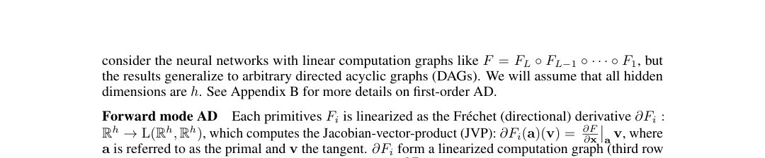
Figure 3: The computation graph of forward mode AD (left) and backward mode AD (right) of a function with primitives each parameterized by . Nodes represent (intermediate) values, and arrows represent computation. Input nodes are colored blue; output nodes are colored green, and intermediate nodes are colored yellow.
图 3:含 4 个原语 (各由 参数化)的函数 的前向模式 AD(左)与反向模式 AD(右)计算图。节点表示(中间)值,箭头表示计算。输入节点蓝色,输出节点绿色,中间节点黄色。
B.2 Derivative via composition
B.2 经复合求导数
First-order AD is based on a simple observation: for a set of functions , the set of tuples of functions and its Jacobian is closed under composition:
一阶 AD 基于简单观察:对函数集 ,函数 与其 Jacobian 组成的元组集合在复合下封闭:
where denotes both function composition and the composition of the tuple . If we have the analytical formula of the Jacobian for every , then we can calculate the Jacobian of any composition of functions from using the above composition rule for the tuple . The set of functions are usually called the primitives.
其中 既表示函数复合,也表示元组 的复合。若对每个 都有 的解析式,即可用上述元组复合规则求 中任意复合的 Jacobian。 中的函数通常称为原语。
B.3 Fréchet derivative and linearization
B.3 Fréchet 导数与线性化
Given normed vector spaces , the Fréchet derivative of a function is a map from to the space of all bounded linear operators from to , denoted as , that is
给定赋范向量空间 ,函数 的 Fréchet 导数 是从 到 到 的全体有界线性算子空间 的映射,即
such that at a point it gives the best linear approximation of , in the sense that
使得在点 处给出 的最佳线性逼近 ,意义为
Therefore, it is also called the linearization of at point . Concretely, consider a function in Euclidean spaces . At any point , the Fréchet derivative can be seen as the directional derivative of :
因此也称 在 处的线性化。具体地,考虑欧氏空间中的 。在任意 , 可视为 的方向导数:
where denote the Jacobian of at point called the primal, and , also called the tangent is a vector representing the direction. Therefore the Fréchet derivative is also called Jacobian-vector-product (JVP). And we can write the truncated Taylor expansion as
其中 是 在主值 处的 Jacobian, 是表示方向的切向量。因此 Fréchet 导数也称 Jacobian–向量积(JVP)。截断 Taylor 展开可写为
Many operators have efficient JVP implementation due to sparsity. For example, element-wise application of scalar function (e.g. activation in neural networks) has diagonal Jacobian, and its JVP can be efficiently implemented as a Hadamard product. Another prominent example is discrete convolution, whose JVP has efficient implementation via FFT.
许多算子因稀疏而有高效 JVP。例如逐元标量函数(如神经网络激活)的 Jacobian 对角,JVP 可高效实现为 Hadamard 积;另一典型例子是离散卷积,其 JVP 可用 FFT 高效实现。
B.4 Adjoint of the Fréchet derivative
B.4 Fréchet 导数的伴随
Given two topological vector spaces , the linear map has an adjoint where are the dual spaces. The adjoint satisfies the following
给定拓扑向量空间 ,线性映射 有伴随 ,其中 为对偶空间。伴随满足
In the finite-dimensional case, the dual space is the space of row vectors, and any linear map can be written as . One can easily verify that the adjoint is the transpose: . The adjoint (transpose) of the Fréchet derivative of , denoted as , is thus defined as
有限维时对偶空间即行向量空间,任意线性映射可写 ;易验证伴随即转置:。于是 的 Fréchet 导数的伴随(转置) 定义为
where is the cotangent which lives in the dual space of the codomain. Note that the adjoint is taken to only where is kept fixed. is also called vector-Jacobian-product (VJP).
其中 是落在值域对偶空间中的余切。注意伴随只对 取,主值 固定。 也称 向量–Jacobian 积(VJP)。
Appendix C Why mixed mode AD schemes like the forward-over-backward might not be better than stacked backward mode AD in the case of PINN
附录 C 为何在 PINN 情形下 Forward-over-backward 等混合模式未必优于堆叠反向模式 AD
In AD literature [9], the second order derivative is recommended to be computed via forward-over-backward AD, i.e., first do a backward mode AD to get the first order derivative, then apply forward mode AD to the first order derivative to obtain the second order derivative. Usually, we will expect that forward-over-backward AD gives better performance in memory usage over stacked backward AD since the outer differential operator has to differentiate a larger computation graph than the inner one, and forward AD has less overhead as explained in section B.2. Essentially, forward-over-backward reverses the arrows in the third row in Fig. 1, therefore reducing the number of sequential computations and also the size of the evaluation trace. However, in the case of PINN, yet another differentiation to the network parameters needs to be taken. So, computing the second-order differential operator here with forward-over-backward AD might not yield any advantage.
AD 文献 [9] 建议用 Forward-over-backward 求二阶导:先反向得一阶导,再对一阶导做前向得二阶导。通常会预期它在显存上优于堆叠反向:外层微分算子要对更大计算图求导,而前向 AD 开销更小(见 B.2 节)。实质上 Forward-over-backward 反转了图 1 第三行的箭头,从而减少串行计算次数与求值轨迹规模。但在 PINN 中还需再对网络参数 求导,因而用 Forward-over-backward 算二阶微分算子未必占优。
Appendix D Taylor mode AD
附录 D Taylor 模式 AD
D.1 High-order Fréchet Derivatives
D.1 高阶 Fréchet 导数
The th order Fréchet derivative of a function at a point is the multi-linear map with arguments around point that best approximates . For example, when , we have
函数 在点 的 阶 Fréchet 导数,是在 附近用 个自变量的多重线性映射对 做最佳逼近。例如 时有
where denote the Hessian of at point , and . We can now write the second-order truncated Taylor series with it
其中 是 在 的 Hessian,。据此可写二阶截断 Taylor 级数
For the more general case, we have
更一般情形有
High-order Fréchet derivative can be seen as the best th order polynomial approximation of by taking all input tangents to be the same :
把所有输入切向量取成同一 时,高阶 Fréchet 导数可视为 的最佳 次多项式逼近:
D.2 Composition rule for high-order Fréchet derivatives
D.2 高阶 Fréchet 导数的复合规则
Next, we derive the higher-order composition rule by repeatedly applying the usual chain rule.
下面反复应用通常链式法则,推导高阶复合规则。
For composition of scalar functions, we can generalize the chain rule for high-order derivatives by iteratively applying the chain rule to lower-order chain rules:
对标量函数复合 ,可通过对低阶链式法则迭代套用链式法则,把链式法则推广到高阶导:
$$\begin{split}\partialderivative{x}f(g(x))=&f^{(1)}(g(x))\cdot g^{(1)}(x)\
\partialderivative[2]{x}f(g(x))=&f^{(1)}(g(x))\cdot g^{(2)}(x)+f^{(2)}(g(x))\cdot[g^{(1)}(x)]^{2}\
\frac{\partial^{3}}{\partial x^{3}}f(g(x))=&f^{(1)}(g(x))\cdot g^{(3)}(x)+3f^{(2)}(g(x))\cdot g^{(1)}(x)\cdot g^{(2)}(x)+f^{(3)}(g(x))\cdot[g^{(1)}(x)]^{3}\end{split} \tag{37}$$
where we give the example of up to the third order. For arbitrary , the th order derivative of the composition is given by the Faa di Bruno’s formula (scalar version)
下面给出到三阶的例子。对任意 ,复合的 阶导由 Faa di Bruno 公式(标量版)给出
$$\partialderivative[k]{x}f(g(x))=\sum_{\begin{subarray}{c}(p_{1},\dots,p_{k})\in\mathbb{N}^{k},\
\sum_{i=1}^{k}i\cdot p_{i}=k\end{subarray}}\frac{k!}{\prod_{i}^{k}p_{i}!(i!)^{p_{i}}}\cdot(f^{(\sum_{i=1}^{n}p_{i})}\circ g)(x)\cdot\prod_{j=1}^{k}\left(\frac{1}{j!}g^{(j)}(x)\right)^{p_{j}}. \tag{38}$$
where the outermost summation is taken over all partitions of the derivative order . Here a partition of is defined as a tuple that satisfies
其中最外层求和取遍导数阶数 的所有分拆。这里 的分拆定义为满足下式的元组
For vector-valued functions , let
对向量值函数 ,令
$$\begin{split}\mathbf{a}=g(\mathbf{x})\in\mathbb{R}^{m},\quad\mathbf{v}^{(1)}=\partialderivative{g(\vb{x})}{\vb{x}}\in\mathbb{R}^{m\times n},\
\mathbf{v}^{(2)}=\partialderivative[2]{g(\vb{x})}{\vb{x}}\in\mathbb{R}^{m\times n\times n},\quad\mathbf{v}^{(3)}=\frac{\partial^{3}g(\mathbf{x})}{\partial\mathbf{x}^{3}}\in\mathbb{R}^{m\times n\times n\times n}\end{split} \tag{40}$$
we can derive the following composition rule similarly
可类似推出如下复合规则
$$\begin{split}\partialderivative{\vb{x}}f(g(\mathbf{x}))=&D_{f}(\mathbf{a}){l,m}v^{(1)}{m,n}\in\mathbb{R}^{l\times n}\
\partialderivative[2]{\vb{x}}f(g(\mathbf{x}))=&D_{f}(\mathbf{a}){l,m}v^{(2)}{m,n,n^{\prime}}+D^{2}{f}(\mathbf{a}){l,m,m^{\prime}}v^{(1)}{m,n}v^{(1)}{m^{\prime},n^{\prime}}\in\mathbb{R}^{l\times n\times n}\
\frac{\partial^{3}}{\partial\mathbf{x}^{3}}f(g(\mathbf{x}))=&D_{f}(\mathbf{a}){l,m}v^{(3)}{m,n,n^{\prime},n^{\prime\prime}}\
+&3\cdot D^{2}{f}(\mathbf{a}){l,m,m^{\prime}}v^{(1)}{m,n}v^{(2)}{m^{\prime},n^{\prime},n^{\prime\prime}}\
+&D^{3}{f}(\mathbf{a}){l,m,m^{\prime},m^{\prime\prime}}v^{(1)}{m,n}v^{(1)}{m^{\prime},n^{\prime}}v^{(1)}_{m^{\prime\prime},n^{\prime\prime}}\in\mathbb{R}^{l\times n\times n\times n}\end{split} \tag{41}$$
where again we give the example of up to the third order, and repeated indexes are summed as in Einstein notation. The general formula is again given by the multivariate version of the Faa di Bruno’s formula. Note that in the multivariate version of the Faa di Bruno’s formula, it is possible to take a derivative to distinguishable variables, but here we just present the version with indistinguishable input variables. This gives the composition rule for th order total derivative.
同样给出到三阶的例子;重复指标按 Einstein 约定求和。一般公式仍由多元版 Faa di Bruno 给出。注意多元版可对可区分变量求导,这里只给出输入变量不可区分的版本,即 阶全导数的复合规则。
The composition of the high-order Fréchet derivative is the case of , as the contraction with the input tangents is the same as composing with a scalar input function with . All derivative tensors of can be represented using a vector, and similarly all derivative tensor of can be represented using a vector. Then, the above chain rule can be simplified to
高阶 Fréchet 导数 的复合对应 的情形:与输入切向量 的收缩,等同于与标量输入函数 ()复合。 的全部导数张量可用 向量表示, 的导数张量 可用 向量表示。于是上述链式法则可简化为
$$\begin{split}\partialderivative{t}f(g(t))=&D_{f}(\mathbf{a}){l,m}v^{(1)}{m}\in\mathbb{R}^{l}\
\partialderivative[2]{t}f(g(t))=&D_{f}(\mathbf{a}){l,m}v^{(2)}{m}+D^{2}{f}(\mathbf{a}){l,m,m^{\prime}}v^{(1)}{m}v^{(1)}{m^{\prime}}\in\mathbb{R}^{l}\
\frac{\partial^{3}}{\partial t^{3}}f(g(t))=&D_{f}(\mathbf{a}){l,m}v^{(3)}{m}+3\cdot D^{2}{f}(\mathbf{a}){l,m,m^{\prime}}v^{(1)}{m}v^{(2)}{m^{\prime}}+D^{3}{f}(\mathbf{a}){l,m,m^{\prime},m^{\prime\prime}}v^{(1)}{m}v^{(1)}{m^{\prime}}v^{(1)}_{m^{\prime\prime}}\in\mathbb{R}^{l}.\end{split} \tag{42}$$
The Faa di Bruno’s formula again gives the general formula for arbitrary derivative order
Faa di Bruno 公式再次给出任意导数阶的一般公式
$$\partialderivative[k]{t}f(g(t))=\sum_{\begin{subarray}{c}(p_{1},\dots,p_{k})\in\mathbb{N}^{k},\
\sum_{i=1}^{k}i\cdot p_{i}=k\end{subarray}}\frac{k!}{\prod_{i}^{k}p_{i}!(i!)^{p_{i}}}\cdot D_{f}^{\sum_{i=1}^{k}p_{i}}(\mathbf{a}){l,m{1},\dots,m_{\sum_{i=1}^{k}p_{i}}}\cdot\prod_{j=1}^{k}\left(\frac{1}{j!}v^{(j)}{m{j}}\right)^{p_{j}}\in\mathbb{R}^{l}. \tag{43}$$
which is written in the perspective of input primal and tangents .
该式从输入主值 与切向量 的视角写出。
Appendix E Removing the mixed partial derivatives term from second order semilinear parabolic PDE
附录 E 从二阶半线性抛物型 PDE 中消去混合偏导项
$$\begin{split}\frac{1}{2}\tr\left(\sigma(\mathbf{x},t)\sigma(\mathbf{x},t)^{\top}(\text{Hess}{\mathbf{x}}u)(\mathbf{x},t)\right)=&\frac{1}{2}\tr\left(\sigma(\mathbf{x},t)^{\top}(\text{Hess}{\mathbf{x}}u)(\mathbf{x},t)\sigma(\mathbf{x},t)\right)\
=&\frac{1}{2}\sum_{i=0}^{d}\left[\sigma(\mathbf{x},t)^{\top}(\text{Hess}{\mathbf{x}}u)(\mathbf{x},t)\sigma(\mathbf{x},t)\right]{i,i}\
=&\frac{1}{2}\sum_{i=0}^{d}\mathbf{e}{i}^{\top}\sigma(\mathbf{x},t)^{\top}(\text{Hess}{\mathbf{x}}u)(\mathbf{x},t)\sigma(\mathbf{x},t)\mathbf{e}{i}\
=&\frac{1}{2}\sum{i=0}^{d}\partial^{2}u((\mathbf{x},t),\sigma(\mathbf{x},t)\mathbf{e}{i},\mathbf{0}^{\top}){[3]}.\end{split} \tag{44}$$
Appendix F Evaluating arbitrary mixed partial derivatives
附录 F 求任意混合偏导
F.1 A concrete example
F.1 一个具体例子
Let’s first consider a concrete case. Suppose the domain is -dimensional we want to compute the mixed derivative . The naive approach would be to compute the entire third order derivative tensor , which is a tensor of shape , then extract the element at index . However note that from Eq. 43, for any , the pushforward of -jet under contains contractions of . Although in the case of , the only contraction of is in the :
先看具体情形。设定义域 维,要求混合导 。朴素做法是算完整三阶导数张量 (形状 ),再取指标 的元。但由式 43,对任意 , 下 -jet 的前推都含 的收缩。虽在 时 的唯一收缩出现在 中:
which can only be used to compute the diagonal or the block diagonal elements, when , we will have a contraction that computes off-diagonal terms, i.e. the mixed partial derivatives. For example, in , if all input tangents are set to zero except for and , becomes:
它只能用来算对角或块对角元;当 时会出现求非对角项(即混合偏导)的收缩。例如在 中,若除 、 外输入切向量皆零,则 变为:
which contains the contraction of that we want:
其中含我们想要的 收缩:
However, there are extra terms. We can remove them by doing two extract pushforwards. We can compute the desired mixed partial derivative with the following pushforward of standard basis:
但仍有多余项。可用两次额外前推消去。用下列标准基前推即可得所需混合偏导:
If we go to higher-order jets, we can use more flexible contractions, and we can compute the mixed derivative with fewer terms to correct, hence less pushforwards. For example, the pushforward of the fifth-order tangent is
若用更高阶 jet,收缩更灵活,纠正项更少,因而前推次数更少。例如五阶切向量的前推为
if all input tangents are set to zero except for and . With this we only need to remove one term:
当除 、 外输入切向量皆零时。此时只需消去一项:
Similarly, by going to the seventh-order tangent, we can compute this mixed derivative with only one pushforward. contains , and when all input tangents are set to zero except for and , equals
类似地,用七阶切向量只需一次前推即可算该混合导。 含 ;当除 、 外皆零时, 等于
which is the exact contraction we want. With this we have
正是我们要的收缩。于是有
F.2 Procedure for finding the right pushforwards for arbitrary mixed partial derivatives
F.2 为任意混合偏导寻找合适前推的流程
More generally, consider the case where we need to compute arbitrary mixed partial derivative
更一般地,设需求任意混合偏导
where is the number of different input dimensions in the mixed partial derivative, and is the order. To compute it with -jet pushforward, one needs to find:
其中 是混合偏导中不同输入维的个数, 是阶数。要用 -jet 前推计算,需找到:
- a derivative order ,
- a sparsity pattern for the tangents of the input jet, which is defined as the tuple of integers where when and for all ,
- 导数阶数 ,
- 输入 jet 切向量 的稀疏模式,定义为 个整数的元组 ,满足 时 ,且对所有 有 ,
such that when setting
使得在设定
$$p_{j}=\left{\begin{array}[]{cc}0,&j\not\in J\
q_{i_{t}},&j=j_{t}\
\end{array}\right., \tag{54}$$
is a partition of as defined in Eq. 39.
是式 39 所定义的 的分拆。
Let’s use the concrete example again. In this case , and . We demonstrated that this can be computed with one -jet pushforward, which is equivalent to setting , , and the partition . The Faa di Bruno’s formula (Eq. 43) ensures that the pushforward of the th order tangent contains a contraction that can be used to compute the desired mixed partial derivative.
仍以 为例。此时 ,,。我们说明可用一次 -jet 前推完成,等价于取 、,分拆 。Faa di Bruno 公式(式 43)保证 阶切向量的前推含可用于计算该混合偏导的收缩。
Furthermore, if there are no other partitions with a sparsity pattern that is the subset of the sparsity pattern of the partition in consideration, there are no extra terms to remove. Intuitively, if a partition has a sparsity pattern that is not a subset, it will vanish when we set the input tangents to zero according to the sparsity pattern of the partition in consideration. To understand this point better, let’s look at the concrete example with the -jet pushforward demonstrated above. and are both valid partition of , and the sparsity pattern of is the subset of that of : are non-zero in both partition. Therefore the pushforward contains extra terms that can be removed with another pushforward. In the example with -jet pushforward, no other partition has the sparsity pattern that is the subset of that of the partition . This is equivalent to say, is the only way to sum up to when you can only use and , which can be verified easily.
进而,若没有其他分拆的稀疏模式是当前分拆稀疏模式的子集,则无需消去多余项。直观上:若某分拆的稀疏模式不是子集,按当前分拆的稀疏模式把输入切向量置零后该项会消失。以先前的 -jet 前推为例: 与 都是 的合法分拆,且 的稀疏模式是 的子集(两者 皆非零),故前推含可用另一次前推消去的多余项。而在 -jet 例子中,没有其他分拆的稀疏模式是 的子集——亦即在只能用 2 与 3 时, 是唯一加到 7 的方式,易验证。
With this setup, it is clear why the diagonal terms can always be computed with pushforward of the lowest possible order: is always a valid partition , and no other partition has sparsity pattern that is a subset of it.
在此设定下,对角项总能用尽可能低阶的前推计算就清楚了: 总是 的合法分拆,且无其他分拆的稀疏模式是它的子集。
For mixed partial derivatives, the difficulty scales the total order of the operator , and which can be interpreted as the degree of the “off-diagonalness” of the operator. For example, consider the case where and . This corresponds to the operator . To avoid overlapping with the diagonal sparsity pattern and to keep the order of derivative low, one might try and the partition . However, with higher , there is more chance that other partitions will have a subset sparsity pattern. In this case is one such example. One will need to either find all the partitions with subset sparsity pattern and remove them with multiple pushforward, or further increase the derivative order to find a pattern with no extra term.
对混合偏导,难度随算子总阶 与可解释为「非对角程度」的 上升。例如 且 ,对应算子 。为避免与对角稀疏模式 重叠并保持导数阶较低,可尝试 与分拆 。但 越高,其他分拆越可能具子集稀疏模式;此处 即为一例。要么找出所有具子集稀疏模式的分拆并用多次前推消去,要么进一步提高导数阶以找到无多余项的模式。
Appendix G Further memory reduction via weight sharing in the first layer
附录 G 经第一层权重共享进一步降显存
When dealing with high-dimensional data, the parameters of the model’s first layer in a conventional fully connected network would grow proportionally with the input dimension, resulting in a significant increase in memory requirements and forming a memory bottleneck due to massive model parameters. To address this issue, convolutional networks are often employed in deep learning for images to reduce the number of model parameters. Here, we adopt a similar approach to mitigate the memory cost of model parameters in high-dimensional PDEs, called weight sharing in the first layer.
处理高维数据时,常规全连接网络第一层参数会随输入维成比例增长,显存急剧上升,形成参数瓶颈。深度学习里对图像常用卷积网络减参;此处对高维 PDE 采用类似思路,称为第一层权重共享。
Denote the input dimension as , which is potentially excessively high, and the hidden dimension of the MLP as , and assume that . The first layer weight is an dimensional matrix, whereas all subsequent layers have a weight matrix with a size of only .
记输入维为 (可能极高)、MLP 隐维为 ,并设 。第一层权重是 矩阵,而后续层权重仅为 。
By introducing a weight-sharing scheme, one can reduce the redundancy in the parameters in the first layer. Specifically, we perform an additional 1D convolution to the input vectors before passing the input into the MLP PINN, as in Fig. 4. The 1D convolution has filter size that divides and stride size , so the convolution output is non-overlapping, and the number of channels is set to .
引入权重共享可降低第一层参数冗余。具体地,在把输入送入 MLP PINN 前,对输入向量 再做一次一维卷积,如图 4。一维卷积滤波器大小 整除 、步长亦为 ,故输出无重叠,通道数设为 1。
This weight-sharing scheme reduces the parameters by approximately . The number of parameters in the filters is , and the subsequent fully connected layer will have a weight matrix of size . Therefore, the total number of the first layer is reduced from to only , and we can see that with a larger block size , we will have fewer parameters, and the reduction factor is approximately . More concretely, suppose where one million () dimensional problems are also tested experimentally, so the number of parameters in the first layer is . If we use a block size of , we will reduce the number of parameters to . If the block size is , the number of parameters will be . In other words, with a larger block size of , we significantly reduce the number of model parameters.
该权重共享约把参数减为原来的 。滤波器参数量为 ,随后全连接层权重为 ;第一层总参数从 降到 ,块大小 越大参数越少,约减因子 。更具体地,设 (实验也测了百万维问题),第一层参数 ;取 则降到 ;取 则为 。亦即更大的 可显著减参。
We will demonstrate the memory efficiency and acceleration thanks to weight-sharing in the experimental section.
实验部分将展示权重共享带来的显存效率与加速。
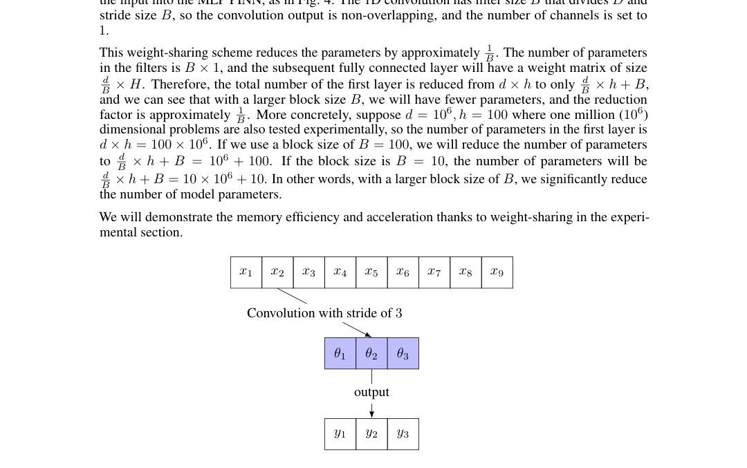
Figure 4: Convolutional weight sharing in the first layer, with input dimension and filter size .
图 4:第一层的卷积权重共享,输入维 ,滤波器大小 。
Appendix H Experiment setup
附录 H 实验设置
Each experiment is run with five different random seeds, and the average and the standard deviations of these runs are reported.
每项实验用五个不同随机种子运行,报告均值与标准差。
To get an accurate reading of memory usage, we use a separate run where GPU memory pre-allocation for JAX is disabled through setting the environment variable XLA_PYTHON_CLIENT_ALLOCATOR=platform, and the test data set is stored on the CPU memory. The GPU memory usage was obtained via NVIDIA-smi and peak memory was reported.
为准确读显存,另开一次运行:通过环境变量 XLA_PYTHON_CLIENT_ALLOCATOR=platform 关闭 JAX 的 GPU 预分配,测试集放在 CPU 显存。GPU 显存经 NVIDIA-smi 读取,报告峰值。
All the experiments were done on a single NVIDIA A100 GPU with 40GB memory and CUDA 12.2. with driver 535.129.03 and JAX version 0.4.23.
全部实验在单块 40GB 显存的 NVIDIA A100 上完成,CUDA 12.2,驱动 535.129.03,JAX 0.4.23。
Network architecture and training hyperparameters
For the semilinear parabolic PDEs tested in Appendix I.2 we follow the network architecture of the original SDGD [13]:
网络结构与训练超参
附录 I.2 中的半线性抛物型 PDE 沿用原 SDGD [13] 的网络结构:
- • The network is a 4-layer multi-layer perceptron (MLP) with 128 hidden units activated by Tanh.
- • The network is trained with Adam [20] for 10K steps, with an initial learning rate of 1e-3 that linearly decays to in 10K steps, where at each step we calculate the model parameters gradient with 100 uniformly sampled random residual points.
- • The model is evaluated using 20K uniformly sampled random points fixed throughout the training.
- • The zero boundary condition is satisfied via the following parameterization (55) where is the MLP network, and is the PDE ansatz, as described in [26].
- • 网络为 4 层 MLP,隐单元 128,Tanh 激活。
- • 用 Adam [20] 训练 10K 步,初始学习率 1e-3,在 10K 步内线性衰减到 ;每步用 100 个均匀采样的随机残差点算参数梯度。
- • 用训练全程固定的 20K 个均匀随机点评估。
- • 零边界条件经如下参数化满足 (55)其中 是 MLP, 是 PDE ansatz,见 [26]。
For the semilinear parabolic PDEs tested in Appendix I.2, we made the following modifications:
对附录 I.2 中的半线性抛物型 PDE,我们做了如下修改:
- • Instead of using re-parameterization, the boundary/initial condition is satisfied by adding a regularization loss to the residual loss: (56) where is the initial data, is the batch size for boundary points, is the PDE ansatz, is the coefficient for the first-order derivative boundary loss term, which we set to . The total loss is (57)
- • Instead of discretizing the time and sample residual points using the underlying stochastic process, we uniformly sample the time steps between the initial and the terminal time, i.e. , and then sample directly from the distribution of , i.e. . To match the original training setting of SDE trajectories with step size for time discretization, we use a batch size of for residual points and for boundary/initial points.
- • We use a 4-layer multi-layer perceptron (MLP) with 1024 hidden units activated by Tanh. The network is trained with Adam [20] for 10K steps, with an initial learning rate of 1e-3 that exponentially decays with exponent .
- • To test the quality of the PINN solution, we measure the relative L1 error at the point against the reference value computed via multilevel Picard’s method [3, 4, 17].
- • 不用重参数化,而是在残差损失上加正则化损失以满足边界/初值: (56)其中 是初值数据, 是边界点批大小, 是 PDE ansatz, 是一阶导边界损失系数,取 。总损失为 (57)
- • 不对时间离散并用底层随机过程采残差点,而是在初末时间间均匀采时间步 ,再直接从 的分布采 。为对齐原设定(100 条 SDE 轨迹、时间离散步长 0.015),残差点批大小 2000,边界/初值点批大小 100。
- • 用 4 层 MLP、隐单元 1024、Tanh;Adam [20] 训练 10K 步,初始学习率 1e-3,指数衰减指数 。
- • 用点 上相对多层 Picard 法 [3, 4, 17] 参考值的相对 L1 误差衡量 PINN 解质量。
In all experiments, we use the biased version of Eq. 25:
全部实验采用式 25 的有偏版本:
as the bias in practice is very small and does not affect convergence.
实践中偏差很小,不影响收敛。
Appendix I Experiments Results
附录 I 实验结果
I.1 Inseparable and effectively high-dimensional PDEs
I.1 不可分且实质高维的 PDE
The first class of PDEs is defined via a nonlinear, inseparable, and effectively high-dimensional exact solution defined within the -dimensional unit ball :
第一类 PDE 由定义在 维单位球 内的非线性、不可分、实质高维精确解 给出:
$$\begin{split}\mathcal{L}u(\mathbf{x})=&f(\mathbf{x}),\quad\mathbf{x}\in\mathbb{B}^{d}\
u(\mathbf{x})=&0,\quad\quad\mathbf{x}\in\partial\mathbb{B}^{d}\end{split} \tag{59}$$
where is a linear/nonlinear operator and . The zero boundary condition ensures that no information about the exact solution is leaked through the boundary condition. We will consider the following operators:
其中 是线性/非线性算子,。零边界条件保证精确解信息不经边界泄漏。我们考虑下列算子:
- • Poisson equation:
- • Allen-Cahn equation:
- • Sine-Gordon equation:
- • Poisson 方程:
- • Allen–Cahn 方程:
- • Sine–Gordon 方程:
For the exact solution, we consider the following with all :
精确解取下列形式,所有 :
- • two-body interaction:
- • three-body interaction:
- • 两体相互作用:
- • 三体相互作用:
We tested the performance of STDE on these equations, and the results are presented in Table 3, 4, 5, 6. For the Allen-Cahn equation, we performed a detailed ablation study (Table 3), and we expect these results to generalize over these second-order PDEs.
我们在这些方程上测试 STDE,结果见表 3、4、5、6。对 Allen–Cahn 做了细消融(表 3),预期这些结果可推广到同类二阶 PDE。
The gain by using JAX instead of PyTorch
Since the original SDGD was implemented in PyTorch, we implemented the stacked backward mode without parallelization in SDGD dimensions in JAX for fair comparison (dubbed as “Stacked Backward mode SDGD in JAX” in Table 3). The for-loop over SDGD dimension is implemented using jax.lax.scan. Table 3 shows that, even with the original stacked backward mode AD, the speed of JAX implementation can be more than 10 faster when the dimension is high. The memory profile is similar. The difference could come from the fact that JAX uses XLA to perform Just-in-time (JIT) compilation of the Python code into optimized kernels. However, note that for the case of 100,000 dimensions, the JAX implementation of the stacked backward mode AD encountered an out-of-memory (OOM) error. This is because performing JIT compilation requires extra memory, and the peak memory requirement during JIT compilation is higher than that during training.
用 JAX 相对 PyTorch 的增益
因原 SDGD 用 PyTorch,为公平比较我们在 JAX 中实现了不对 SDGD 维并行化的堆叠反向模式(表 3 记为「JAX 中的堆叠反向模式 SDGD」)。对 SDGD 维的 for 循环用 jax.lax.scan。表 3 显示:即便仍用原堆叠反向 AD,高维时 JAX 实现也可快逾 10 倍;显存画像相近。差异可能来自 JAX 用 XLA 把 Python 即时编译为优化内核。但注意在 100,000 维时 JAX 堆叠反向 OOM——JIT 编译需额外显存,峰值高于训练时。
Randomization batch size
We also tested the case where the STDE randomization batch size is reduced to . As seen in Table 3, in the case of Allen-Cahn provides 2 speed up, without hurting performance. However, theoretically lowering the randomization batch size leads to higher variance. The trade-off between computational efficiency and stability in convergence warrants further studies.
随机化批大小
我们也测了把 STDE 随机化批大小降到 的情形。表 3 显示对 Allen–Cahn 约加速 2 倍且不伤性能;但理论上减小批大小会增大方差。计算效率与收敛稳定性的权衡值得进一步研究。
| Method | Metric | 100 D | 1K D | 10K D | 100K D | 1M D |
|---|---|---|---|---|---|---|
| Backward mode SDGD (PyTorch) [13] | Speed | 55.56it/s | 3.70it/s | 1.85it/s | 0.23it/s | OOM |
| Memory | 1328MB | 1788MB | 4527MB | 32777MB | OOM | |
| Error | 7.187E-03 | 5.615E-04 | 1.864E-03 | 2.178E-03 | OOM | |
| Backward mode SDGD (JAX) | Speed | 40.63it/s | 37.04it/s | 29.85it/s | OOM | OOM |
| Memory | 553MB | 565MB | 1217MB | OOM | OOM | |
| Error | 3.51E-03 8.47E-05 | 7.29E-04 5.45E-06 | 3.46E-03 2.01E-04 | OOM | OOM | |
| Parallelized backward mode SDGD | Speed | 1376.84it/s | 845.21it/s | 216.83it/s | 29.24it/s | OOM |
| Memory | 539MB | 579MB | 1177MB | 4931MB | OOM | |
| Error | 6.87E-03 6.97E-05 | 3.12E-03 7.04E-04 | 2.59E-03 2.20E-05 | 1.60E-03 1.13E-05 | OOM | |
| Forward-over -Backward SDGD | Speed | 778.18it/s | 560.91it/s | 193.91it/s | 27.18it/s | OOM |
| Memory | 537MB | 579MB | 1519MB | 4929MB | OOM | |
| Error | 4.07E-03 7.42E-05 | 2.19E-03 2.03E-04 | 5.47E-04 7.48E-05 | 4.21E-03 2.53E-04 | OOM | |
| Forward Laplacian [24] | Speed | 1974.50it/s | 373.73it/s | 32.15it/s | OOM | OOM |
| Memory | 507MB | 913MB | 5505MB | OOM | OOM | |
| Error | 4.33E-03 4.97E-05 | 5.50E-04 4.60E-05 | 5.58E-03 2.73E-04 | OOM | OOM | |
| STDE | Speed | 1035.09it/s | 1054.39it/s | 454.16it/s | 156.90it/s | 13.61it/s |
| Memory | 543MB | 537MB | 795MB | 1073MB | 6235MB | |
| Error | 1.03E-02 7.69E-05 | 6.21E-04 2.22E-04 | 3.45E-03 1.17E-05 | 2.59E-03 7.93E-06 | 1.38E-03 3.34E-05 | |
| STDE (batch size=) | Speed | 1833.78it/s | 1559.36it/s | 587.60it/s | 283.33it/s | 21.34it/s |
| Memory | 457MB | 481MB | 741MB | 1063MB | 6295MB | |
| Error | 1.89E-02 2.37E-04 | 7.07E-04 1.02E-05 | 8.33E-04 2.96E-04 | 1.50E-03 1.02E-05 | 3.99E-03 3.41E-05 |
Table 3: Computational results for the Inseparable Allen-Cahn equation with the two-body exact solution, where the randomization batch size is set to unless stated otherwise.
| 方法 | 指标 | 100 D | 1K D | 10K D | 100K D | 1M D |
|---|---|---|---|---|---|---|
| 反向模式 SDGD (PyTorch) [13] | 速度 | 55.56it/s | 3.70it/s | 1.85it/s | 0.23it/s | OOM |
| 显存 | 1328MB | 1788MB | 4527MB | 32777MB | OOM | |
| 误差 | 7.187E-03 | 5.615E-04 | 1.864E-03 | 2.178E-03 | OOM | |
| 反向模式 SDGD (JAX) | 速度 | 40.63it/s | 37.04it/s | 29.85it/s | OOM | OOM |
| 显存 | 553MB | 565MB | 1217MB | OOM | OOM | |
| 误差 | 3.51E-03 8.47E-05 | 7.29E-04 5.45E-06 | 3.46E-03 2.01E-04 | OOM | OOM | |
| 并行化反向模式 SDGD | 速度 | 1376.84it/s | 845.21it/s | 216.83it/s | 29.24it/s | OOM |
| 显存 | 539MB | 579MB | 1177MB | 4931MB | OOM | |
| 误差 | 6.87E-03 6.97E-05 | 3.12E-03 7.04E-04 | 2.59E-03 2.20E-05 | 1.60E-03 1.13E-05 | OOM | |
| Forward-over-Backward SDGD | 速度 | 778.18it/s | 560.91it/s | 193.91it/s | 27.18it/s | OOM |
| 显存 | 537MB | 579MB | 1519MB | 4929MB | OOM | |
| 误差 | 4.07E-03 7.42E-05 | 2.19E-03 2.03E-04 | 5.47E-04 7.48E-05 | 4.21E-03 2.53E-04 | OOM | |
| Forward Laplacian [24] | 速度 | 1974.50it/s | 373.73it/s | 32.15it/s | OOM | OOM |
| 显存 | 507MB | 913MB | 5505MB | OOM | OOM | |
| 误差 | 4.33E-03 4.97E-05 | 5.50E-04 4.60E-05 | 5.58E-03 2.73E-04 | OOM | OOM | |
| STDE | 速度 | 1035.09it/s | 1054.39it/s | 454.16it/s | 156.90it/s | 13.61it/s |
| 显存 | 543MB | 537MB | 795MB | 1073MB | 6235MB | |
| 误差 | 1.03E-02 7.69E-05 | 6.21E-04 2.22E-04 | 3.45E-03 1.17E-05 | 2.59E-03 7.93E-06 | 1.38E-03 3.34E-05 | |
| STDE(批大小=) | 速度 | 1833.78it/s | 1559.36it/s | 587.60it/s | 283.33it/s | 21.34it/s |
| 显存 | 457MB | 481MB | 741MB | 1063MB | 6295MB | |
| 误差 | 1.89E-02 2.37E-04 | 7.07E-04 1.02E-05 | 8.33E-04 2.96E-04 | 1.50E-03 1.02E-05 | 3.99E-03 3.41E-05 |
表 3:不可分 Allen–Cahn 方程(两体精确解)的计算结果;除另说明外随机化批大小为 。
| Method | Metric | 100D | 1K D | 10K D | 100K D | 1M D |
|---|---|---|---|---|---|---|
| Backward mode SDGD (PyTorch) [13] | Speed | 55.56it/s | 3.70it/s | 1.85it/s | 0.23it/s | OOM |
| Memory | 1328MB | 1788MB | 4527MB | 32777MB | OOM | |
| Error | 7.189E-03 | 5.611E-04 | 1.850E-03 | 2.175E-03 | OOM | |
| STDE (batch size=) | Speed | 2020.05it/s | 1649.20it/s | 584.98it/s | 281.78it/s | 20.38it/s |
| Memory | 457MB | 481MB | 741MB | 1063MB | 6295MB | |
| Error | 3.50E-03 1.44E-04 | 4.91E-04 3.45E-05 | 4.70E-03 2.10E-05 | 3.49E-03 2.14E-05 | 9.18E-04 6.39E-06 |
Table 4: Computational results for the Inseparable Poisson equation with two-body exact solution.
| 方法 | 指标 | 100D | 1K D | 10K D | 100K D | 1M D |
|---|---|---|---|---|---|---|
| 反向模式 SDGD (PyTorch) [13] | 速度 | 55.56it/s | 3.70it/s | 1.85it/s | 0.23it/s | OOM |
| 显存 | 1328MB | 1788MB | 4527MB | 32777MB | OOM | |
| 误差 | 7.189E-03 | 5.611E-04 | 1.850E-03 | 2.175E-03 | OOM | |
| STDE(批大小=) | 速度 | 2020.05it/s | 1649.20it/s | 584.98it/s | 281.78it/s | 20.38it/s |
| 显存 | 457MB | 481MB | 741MB | 1063MB | 6295MB | |
| 误差 | 3.50E-03 1.44E-04 | 4.91E-04 3.45E-05 | 4.70E-03 2.10E-05 | 3.49E-03 2.14E-05 | 9.18E-04 6.39E-06 |
表 4:不可分 Poisson 方程(两体精确解)的计算结果。
| Method | Metric | 100 D | 1K D | 10K D | 100K D | 1M D |
|---|---|---|---|---|---|---|
| Backward mode SDGD (PyTorch) [13] | Speed | 55.56it/s | 3.70it/s | 1.85it/s | 0.23it/s | OOM |
| Memory | 1328MB | 1788MB | 4527MB | 32777MB | OOM | |
| Error | 7.192E-03 | 5.641E-04 | 1.854E-03 | 2.177E-03 | OOM | |
| STDE (batch size=) | Speed | 1926.33it/s | 1467.38it/s | 566.26it/s | 279.24it/s | 19.88it/s |
| Memory | 457MB | 481MB | 741MB | 1063MB | 6295MB | |
| Error | 3.64E-03 1.46E-04 | 5.40E-04 7.21E-05 | 5.32E-03 5.12E-04 | 9.56E-04 8.03E-06 | 9.47E-04 8.30E-06 |
Table 5: Computational results for the Inseparable Sine-Gordon equation with two-body exact solution.
| 方法 | 指标 | 100 D | 1K D | 10K D | 100K D | 1M D |
|---|---|---|---|---|---|---|
| 反向模式 SDGD (PyTorch) [13] | 速度 | 55.56it/s | 3.70it/s | 1.85it/s | 0.23it/s | OOM |
| 显存 | 1328MB | 1788MB | 4527MB | 32777MB | OOM | |
| 误差 | 7.192E-03 | 5.641E-04 | 1.854E-03 | 2.177E-03 | OOM | |
| STDE(批大小=) | 速度 | 1926.33it/s | 1467.38it/s | 566.26it/s | 279.24it/s | 19.88it/s |
| 显存 | 457MB | 481MB | 741MB | 1063MB | 6295MB | |
| 误差 | 3.64E-03 1.46E-04 | 5.40E-04 7.21E-05 | 5.32E-03 5.12E-04 | 9.56E-04 8.03E-06 | 9.47E-04 8.30E-06 |
表 5:不可分 Sine–Gordon 方程(两体精确解)的计算结果。
| Eq. | Metric | 100 D | 1K D | 10K D | 100K D | 1M D |
|---|---|---|---|---|---|---|
| Allen-Cahn | Speed | 1938.80it/s | 1840.21it/s | 1291.67it/s | 356.76it/s | 46.97it/s |
| Memory | 461MB | 481MB | 539MB | 1055MB | 6233MB | |
| Error | 9.97E-03 3.89E-04 | 1.43E-03 1.60E-04 | 6.21E-04 8.15E-05 | 1.56E-05 3.28E-07 | 2.25E-06 1.48E-07 | |
| Poisson * | Speed | 1991.28it/s | 1872.31it/s | 1276.21it/s | 364.04it/s | 31.73it/s |
| Memory | 473MB | 481MB | 539MB | 1055MB | 6233MB | |
| Error | 1.00E-02 3.27E-04 | 1.02E-03 3.67E-05 | 1.01E-04 2.40E-07 | 9.26E-02 5.36E-04 | 4.82E-06 2.16E-07 | |
| Sine-Gordon | Speed | 1938.80it/s | 1840.21it/s | 1291.67it/s | 356.76it/s | 46.88it/s |
| Memory | 475MB | 479MB | 539MB | 1063MB | 6233MB | |
| Error | 9.97E-03 3.89E-04 | 1.43E-03 1.60E-04 | 6.21E-04 8.15E-05 | 1.56E-05 3.28E-07 | 2.31E-05 1.48E-06 |
Table 6: Computational results for the Inseparable Allen-Cahn, Poisson, and Sine-Gordon equation with the three-body exact solution, computed via STDE with randomization batch size set to . *STDE with randomization batch size () of performs poorly on the 1M dimensional Inseparable Poisson equation with three-body exact solution: the L2 relative error is only 9.05E-02 6.88E-04. To get better convergence, we increase the randomization batch size to for the 1M case. This incurs no extra memory cost and is only slightly slower than the original setting (speed is 46.80it/s when randomization batch size is ).
| 方程 | 指标 | 100 D | 1K D | 10K D | 100K D | 1M D |
|---|---|---|---|---|---|---|
| Allen–Cahn | 速度 | 1938.80it/s | 1840.21it/s | 1291.67it/s | 356.76it/s | 46.97it/s |
| 显存 | 461MB | 481MB | 539MB | 1055MB | 6233MB | |
| 误差 | 9.97E-03 3.89E-04 | 1.43E-03 1.60E-04 | 6.21E-04 8.15E-05 | 1.56E-05 3.28E-07 | 2.25E-06 1.48E-07 | |
| Poisson * | 速度 | 1991.28it/s | 1872.31it/s | 1276.21it/s | 364.04it/s | 31.73it/s |
| 显存 | 473MB | 481MB | 539MB | 1055MB | 6233MB | |
| 误差 | 1.00E-02 3.27E-04 | 1.02E-03 3.67E-05 | 1.01E-04 2.40E-07 | 9.26E-02 5.36E-04 | 4.82E-06 2.16E-07 | |
| Sine–Gordon | 速度 | 1938.80it/s | 1840.21it/s | 1291.67it/s | 356.76it/s | 46.88it/s |
| 显存 | 475MB | 479MB | 539MB | 1063MB | 6233MB | |
| 误差 | 9.97E-03 3.89E-04 | 1.43E-03 1.60E-04 | 6.21E-04 8.15E-05 | 1.56E-05 3.28E-07 | 2.31E-05 1.48E-06 |
表 6:不可分 Allen–Cahn、Poisson、Sine–Gordon 方程(三体精确解)经 STDE、随机化批大小 的结果。*STDE 在批大小 16 时对百万维不可分 Poisson(三体)表现差:L2 相对误差仅 9.05E-026.88E-04。为更好收敛,百万维情形把批大小增到 50;不增额外显存,仅略慢于原设定(批大小 16 时速度 46.80it/s)。
I.2 Semilinear Parabolic PDEs
I.2 半线性抛物型 PDE
The second class of PDEs is the semilinear parabolic PDEs, where the initial condition is specified:
第二类是半线性抛物型 PDE,初值给定:
$$\begin{split}\partialderivative{t}u(\mathbf{x},t)=&\mathcal{L}u(\mathbf{x},t)\quad(\mathbf{x},t)\in\mathbb{R}^{d}\times[0,T]\
u(\mathbf{x},t)=&g(\mathbf{x}),\quad(\mathbf{x},t)\in\mathbb{R}^{d}\times{0}\end{split} \tag{60}$$
where is a known, analytical, and time-independent function that specifies the initial condition, and is the terminal time. We aim to approximate the solution’s true value at one test point , at the terminal time , i.e. at .
其中 是已知、解析、与时间无关的初值函数, 是终端时刻。目标是逼近测试点 在终端时刻 ,即点 上的真解。
We will consider the following operators
我们考虑下列算子
- • Semilinear Heat Eq. (61) with initial condition ,
- • Allen-Cahn equation (62) with initial condition ,
- • Sine-Gordon equation (63) with initial condition ,
- • 半线性热方程 (61)初值 ,
- • Allen–Cahn 方程 (62)初值 ,
- • Sine–Gordon 方程 (63)初值 ,
All three equation uses the test point and terminal time .
三个方程均用测试点 、终端时刻 。
| Method | Metric | 10 D | 100 D | 1K D | 10K D |
|---|---|---|---|---|---|
| Backward mode SDGD (PyTorch) [13] | Speed | - | - | - | - |
| Memory | - | - | - | - | |
| Error | 1.052E-03 | 5.263E-04 | 6.910E-03 | 1.598E-03 | |
| BackwardBackward mode SDGD (JAX) | Speed | 211.63it/s | 207.66it/s | 188.31it/s | 93.21it/s |
| Memory | 619MB | 621MB | 655MB | 1371MB | |
| Error | 8.55E-05 6.75E-05 | 4.02E-04 2.07E-04 | 3.81E-04 4.43E-04 | 2.60E-03 1.38E-03 | |
| STDE | Speed | 660.82it/s | 635.16it/s | 599.15it/s | 361.11it/s |
| Memory | 625MB | 625MB | 657MB | 971MB | |
| Error | 6.99E-05 5.78E-05 | 3.69E-04 2.19E-04 | 3.38E-04 3.30E-04 | 6.08E-03 7.47E-03 |
Table 7: Computational results for the Time-dependent Semilinear Heat equation, where the number of SDGD sampled dimensions is set to .
| 方法 | 指标 | 10 D | 100 D | 1K D | 10K D |
|---|---|---|---|---|---|
| 反向模式 SDGD (PyTorch) [13] | 速度 | - | - | - | - |
| 显存 | - | - | - | - | |
| 误差 | 1.052E-03 | 5.263E-04 | 6.910E-03 | 1.598E-03 | |
| 反向模式 SDGD (JAX) | 速度 | 211.63it/s | 207.66it/s | 188.31it/s | 93.21it/s |
| 显存 | 619MB | 621MB | 655MB | 1371MB | |
| 误差 | 8.55E-05 6.75E-05 | 4.02E-04 2.07E-04 | 3.81E-04 4.43E-04 | 2.60E-03 1.38E-03 | |
| STDE | 速度 | 660.82it/s | 635.16it/s | 599.15it/s | 361.11it/s |
| 显存 | 625MB | 625MB | 657MB | 971MB | |
| 误差 | 6.99E-05 5.78E-05 | 3.69E-04 2.19E-04 | 3.38E-04 3.30E-04 | 6.08E-03 7.47E-03 |
表 7:含时半线性热方程结果;SDGD 采样维数设为 。
| Method | Metric | 10 D | 100 D | 1K D | 10K D |
|---|---|---|---|---|---|
| BackwardBackward mode SDGD (PyTorch) [13] | Speed | - | - | - | - |
| Memory | - | - | - | - | |
| Error | 7.815E-04 | 3.142E-04 | 7.042E-04 | 2.477E-04 | |
| Backward mode SDGD (JAX) | Speed | 211.38it/s | 206.42it/s | 188.02it/s | 93.20it/s |
| Memory | 619MB | 621MB | 657MB | 1371MB | |
| Error | 6.31E-02 3.79E-02 | 4.38E-03 2.48E-03 | 1.35E-03 1.23E-03 | 3.97E-04 3.03E-04 | |
| STDE | Speed | 677.51it/s | 650.98it/s | 598.33it/s | 361.31it/s |
| Memory | 533MB | 535MB | 657MB | 903MB | |
| Error | 6.37E-02 3.77E-02 | 4.38E-03 2.47E-03 | 1.26E-03 1.29E-03 | 3.79E-04 2.75E-04 |
Table 8: Computational results for the Time-dependent Allen-Cahn equation, where the number of SDGD sampled dimensions is set to .
| 方法 | 指标 | 10 D | 100 D | 1K D | 10K D |
|---|---|---|---|---|---|
| 反向模式 SDGD (PyTorch) [13] | 速度 | - | - | - | - |
| 显存 | - | - | - | - | |
| 误差 | 7.815E-04 | 3.142E-04 | 7.042E-04 | 2.477E-04 | |
| 反向模式 SDGD (JAX) | 速度 | 211.38it/s | 206.42it/s | 188.02it/s | 93.20it/s |
| 显存 | 619MB | 621MB | 657MB | 1371MB | |
| 误差 | 6.31E-02 3.79E-02 | 4.38E-03 2.48E-03 | 1.35E-03 1.23E-03 | 3.97E-04 3.03E-04 | |
| STDE | 速度 | 677.51it/s | 650.98it/s | 598.33it/s | 361.31it/s |
| 显存 | 533MB | 535MB | 657MB | 903MB | |
| 误差 | 6.37E-02 3.77E-02 | 4.38E-03 2.47E-03 | 1.26E-03 1.29E-03 | 3.79E-04 2.75E-04 |
表 8:含时 Allen–Cahn 方程结果;SDGD 采样维数设为 。
| Method | Metric | 10 D | 100 D | 1K D | 10K D |
|---|---|---|---|---|---|
| BackwardBackward mode SDGD (PyTorch) [13] | Speed | - | - | - | - |
| Memory | - | - | - | - | |
| Error | 7.815E-04 | 3.142E-04 | 7.042E-04 | 2.477E-04 | |
| BackwardBackward mode SDGD (JAX) | Speed | 210.83it/s | 207.44it/s | 187.98it/s | 93.17it/s |
| Memory | 619MB | 621MB | 655MB | 1371MB | |
| Error | 5.39E-05 4.10E-05 | 9.15E-05 6.06E-05 | 4.19E-04 2.18E-04 | 3.74E-02 4.15E-02 | |
| STDE | Speed | 629.04it/s | 608.83it/s | 596.12it/s | 365.09it/s |
| Memory | 525MB | 539MB | 655MB | 971MB | |
| Error | 4.15E-05 3.21E-05 | 2.54E-04 1.76E-04 | 4.05E-03 1.44E-02 | 1.66E-02 5.95E-03 |
Table 9: Computational results for the Time-dependent Sine-Gordon equation, where the number of SDGD sampled dimensions is set to .
| 方法 | 指标 | 10 D | 100 D | 1K D | 10K D |
|---|---|---|---|---|---|
| 反向模式 SDGD (PyTorch) [13] | 速度 | - | - | - | - |
| 显存 | - | - | - | - | |
| 误差 | 7.815E-04 | 3.142E-04 | 7.042E-04 | 2.477E-04 | |
| 反向模式 SDGD (JAX) | 速度 | 210.83it/s | 207.44it/s | 187.98it/s | 93.17it/s |
| 显存 | 619MB | 621MB | 655MB | 1371MB | |
| 误差 | 5.39E-05 4.10E-05 | 9.15E-05 6.06E-05 | 4.19E-04 2.18E-04 | 3.74E-02 4.15E-02 | |
| STDE | 速度 | 629.04it/s | 608.83it/s | 596.12it/s | 365.09it/s |
| 显存 | 525MB | 539MB | 655MB | 971MB | |
| 误差 | 4.15E-05 3.21E-05 | 2.54E-04 1.76E-04 | 4.05E-03 1.44E-02 | 1.66E-02 5.95E-03 |
表 9:含时 Sine–Gordon 方程结果;SDGD 采样维数设为 。
I.3 Weight sharing
I.3 权重共享
We tested the weight-sharing technique mentioned in Section G.
我们测试了附录 G 所述的权重共享技术。
In this section, we evaluate the performance of the weight-sharing scheme described in Appendix G. We tested the best-performing method from Table 3 (STDE with small randomization batch size of ) with different weight-sharing block sizes, on the inseparable Allen-Cahn equation with the two-body exact solution.
本节评估附录 G 的权重共享方案。在不可分 Allen–Cahn(两体精确解)上,用表 3 最佳方法(STDE,随机化批大小 16)测试不同权重共享块大小。
From Table 10, we can see that weight sharing drastically reduces the number of network parameters and memory usage. With , there is a x reduction in memory and there is no performance loss in terms of L2 relative error.
由表 10,权重共享大幅降低网络参数量与显存。 时显存约降 2.5 倍,且 L2 相对误差无损失。
However, from the experiments we can see that, in both the 1M and the 5M case, increasing the block size beyond provides diminishing returns. For the 1M case, increasing to affects the convergence quality, as the L2 relative error goes up by x. For 5M, the maximum block size one can use before degrading performance is , which is expected as the dimensionality of the problem is higher.
但实验也显示:在 1M 与 5M 情形,块大小超过 50 后收益递减。1M 时把 增到 1000 会伤收敛,L2 相对误差升约 100 倍;5M 时不伤性能的最大块大小为 500——问题维数更高,符合预期。
From Table 10 we can also see that in the M-dimensional case, we will have an out-of-memory (OOM) error without weight sharing. With weight sharing enabled, we can effectively solve the M-dimensional PDE with good relative L2 error, in around minutes.
表 10 还显示:5M 维时若不做权重共享会 OOM;启用后可有效求解 5M 维 PDE,相对 L2 误差良好,约 30 分钟。
| dim | |||||||
|---|---|---|---|---|---|---|---|
| 1M | Speed | 21.34it/s | 16.67it/s | 23.14it/s | 23.73it/s | 25.47it/s | 26.60it/s |
| Memory | 6295MB | 4819MB | 2505MB | 2461MB | 2409MB | 2403MB | |
| #Param. | 128,033,281 | 12,833,292 | 2,593,332 | 1,313,382 | 289,782 | 162,282 | |
| Error | 3.99E-03 3.41E-05 | 1.86E-02 3.13E-04 | 4.76E-03 1.27E-04 | 1.22E-03 6.05E-05 | 2.57E-03 1.15E-04 | 6.06E-01 4.17E-04 | |
| 5M | Speed | OOM | 3.16it/s | 4.47it/s | 4.74it/s | 4.82it/s | 4.76it/s |
| Memory | OOM | 25023MB | 10595MB | 10359MB | 10163MB | 10143MB | |
| #Param. | 640,033,281 | 64,033,292 | 12,833,332 | 6,433,382 | 1,313,782 | 674,282 | |
| Error | OOM | 5.11E-01 4.01E-04 | 3.13E-03 2.34E-04 | 3.94E-03 2.22E-04 | 1.98E-03 5.20E-05 | 6.27E-01 3.03E-04 |
Table 10: Effects of different weight sharing block sizes for the Inseparable Allen-Cahn equation with two-body exact solution solved with STDE with randomization batch size of . equals no weight sharing.
| 维数 | |||||||
|---|---|---|---|---|---|---|---|
| 1M | 速度 | 21.34it/s | 16.67it/s | 23.14it/s | 23.73it/s | 25.47it/s | 26.60it/s |
| 显存 | 6295MB | 4819MB | 2505MB | 2461MB | 2409MB | 2403MB | |
| 参数量 | 128,033,281 | 12,833,292 | 2,593,332 | 1,313,382 | 289,782 | 162,282 | |
| 误差 | 3.99E-03 3.41E-05 | 1.86E-02 3.13E-04 | 4.76E-03 1.27E-04 | 1.22E-03 6.05E-05 | 2.57E-03 1.15E-04 | 6.06E-01 4.17E-04 | |
| 5M | 速度 | OOM | 3.16it/s | 4.47it/s | 4.74it/s | 4.82it/s | 4.76it/s |
| 显存 | OOM | 25023MB | 10595MB | 10359MB | 10163MB | 10143MB | |
| 参数量 | 640,033,281 | 64,033,292 | 12,833,332 | 6,433,382 | 1,313,782 | 674,282 | |
| 误差 | OOM | 5.11E-01 4.01E-04 | 3.13E-03 2.34E-04 | 3.94E-03 2.22E-04 | 1.98E-03 5.20E-05 | 6.27E-01 3.03E-04 |
表 10:不可分 Allen–Cahn(两体精确解)上不同权重共享块大小 的影响;STDE 随机化批大小为 。 即无权重共享。
I.4 High-order PDEs
I.4 高阶 PDE
Here we demonstrate how to use STDE to calculate mixed partial derivatives in some actual PDE. We will consider the 2D Korteweg-de Vries (KdV) equation and the 2D Kadomtsev-Petviashvili equation from [32], and the regular 1D KdV equation with gPINN [42].
下面展示如何用 STDE 计算实际 PDE 中的混合偏导。考虑 [32] 的二维 Korteweg–de Vries(KdV)与二维 Kadomtsev–Petviashvili 方程,以及带 gPINN [42] 的常规一维 KdV。
We will demonstrate that STDE increases the speed for computing the mixed partial derivatives, as it avoids computing the entire derivative tensor. Since these equations are low-dimensional we do not need to sample over the space dimension.
我们将说明 STDE 通过避免算完整导数张量,加快混合偏导计算。这些方程维数低,无需在空间维上采样。
In this section, the equations are all time-dependent and the space is 2D, and we will omit the argument to the solution, i.e. we will write . To test the speed improvement, we run the STDE implementation against repeated backward mode AD on a Nvidia A100 GPU with 40GB memory. The results are reported in Table 11. From the Table we see that STDE provides around 2 speed up compared to repeated application of backward mode AD across different network sizes.
本节方程均含时、空间二维,省略解的自变量,即写 。为测加速,在 40GB NVIDIA A100 上对比 STDE 与反复反向模式 AD,结果见表 11。表中显示跨不同网络规模,STDE 相对反复反向约加速 2 倍。
Alternative way to compute the terms in 2D Korteweg-de Vries (KdV) equation
The terms in the 2D KdV equation
计算二维 Korteweg–de Vries(KdV)方程各项的另一种方式
二维 KdV 方程中的各项
can alternatively be computed with the pushforward of the following jets
也可由下列 jet 的前推计算
All the derivative terms can be found in these output jets :
所有导数项都可在这些输出 jet 中找到:
2D Kadomtsev-Petviashvili (KP) equation
Consider the following equation
二维 Kadomtsev–Petviashvili(KP)方程
考虑如下方程
which can be expanded as
可展开为
All the derivative terms can be computed with a 5-jet, 4-jet, and a 2-jet pushforward. Let
所有导数项可用一次 5-jet、一次 4-jet 与一次 2-jet 前推计算。令
Then all required derivative terms can be evaluated as follows.
则所需导数项可如下求值。
Gradient-enhanced 1D Korteweg-de Vries (g-KdV) equation
Consider the following equation
梯度增强的一维 Korteweg–de Vries(g-KdV)方程
考虑如下方程
Gradient-enhanced PINN (gPINN) [42] regularizes the learned PINN such that the gradient of the residual is close to the zero vector. This increases the accuracy of the solution. Specifically, the PINN loss (Eq. 24) is augmented with the term
梯度增强 PINN(gPINN)[42] 正则化所学 PINN,使残差梯度接近零向量,从而提高解精度。具体地,在 PINN 损失(式 24)上增加项
The total loss becomes
总损失变为
where is the g-PINN penalty weight. To perform gradient-enhancement we need to compute the gradient of the residual:
其中 是 g-PINN 惩罚权重。做梯度增强需计算残差梯度:
$$\begin{split}R(x,t):=u_{t}+uu_{x}+\alpha u_{xxx},\
\nabla R(x,t)=\matrixquantity[\lx@physics@matrix
u_{t t} + u_{t}u_{x} + uu_{t x} + \alpha u_{t x x x }, &
u_{t x} + u_{x}u_{x} + uu_{xx} + \alpha u_{x x x x}
\endlx@physics@matrix].\end{split} \tag{74}$$
All the derivative terms can be computed with one 2-jet and two 7-jet pushforward. Let
所有导数项可用一次 2-jet 与两次 7-jet 前推计算。令
Then all required derivative terms can be evaluated as follows.
则所需导数项可如下求值。
| Speed (it/s) | network size | Base | |||||
|---|---|---|---|---|---|---|---|
| 2D KdV | Backward | 762.86 | 279.19 | 123.20 | 656.01 | 541.10 | 349.23 |
| STDE | 1372.41 | 642.82 | 303.39 | 1209.30 | 743.75 | 418.13 | |
| STDE* | 1357.64 | 606.43 | 272.01 | 1203.97 | 841.07 | 442.32 | |
| 2D KP | Backward | 766.79 | 278.53 | 123.67 | 642.34 | 525.23 | 340.94 |
| STDE | 1518.82 | 676.16 | 304.95 | 1498.61 | 1052.62 | 642.21 | |
| 1D g-KdV | Backward | 621.04 | 232.35 | 102.39 | 559.65 | 482.52 | 293.97 |
| STDE | 1307.27 | 593.21 | 253.48 | 1187.31 | 776.65 | 441.50 |
Table 11: Speed scaling for training low-dimensional high-order PDEs with different network sizes. The base network has depth and width . STDE* is the alternative scheme using lower-order pushforwards.
| 速度 (it/s) | 网络规模 | Base | |||||
|---|---|---|---|---|---|---|---|
| 2D KdV | 反向 | 762.86 | 279.19 | 123.20 | 656.01 | 541.10 | 349.23 |
| STDE | 1372.41 | 642.82 | 303.39 | 1209.30 | 743.75 | 418.13 | |
| STDE* | 1357.64 | 606.43 | 272.01 | 1203.97 | 841.07 | 442.32 | |
| 2D KP | 反向 | 766.79 | 278.53 | 123.67 | 642.34 | 525.23 | 340.94 |
| STDE | 1518.82 | 676.16 | 304.95 | 1498.61 | 1052.62 | 642.21 | |
| 1D g-KdV | 反向 | 621.04 | 232.35 | 102.39 | 559.65 | 482.52 | 293.97 |
| STDE | 1307.27 | 593.21 | 253.48 | 1187.31 | 776.65 | 441.50 |
表 11:不同网络规模下训练低维高阶 PDE 的速度缩放。基础网络深度 、宽度 。STDE* 为用更低阶前推的替代方案。
I.4.2 Amortized gradient-enhanced PINN for high-dimensional PDEs
It is expensive to apply gradient enhancement for high-dimensional PDEs. For example, the gradient of the residual for the inseparable Allen-Cahn equation described in I.1 is given by
I.4.2 高维 PDE 的摊销梯度增强 PINN
对高维 PDE 做梯度增强代价很高。例如 I.1 中不可分 Allen–Cahn 的残差梯度为
With STDE randomization, we randomized the second order term with index sampled from . We can also sample the gPINN penalty terms. As mentioned in Appendix F.1, we have
用 STDE 随机化时,我们对二阶项 从 采样指标 ;也可对 gPINN 惩罚项采样。如附录 F.1 所述,有
We further have
进一步有
so the STDE of the Laplacian operator can be computed together with the above pushforward. With this pushforward, we can efficiently amortize the gPINN regularization loss by minimizing the following upperbound on the original gPINN loss with randomized Laplacian
因而 Laplace 算子的 STDE 可与上述前推一并计算。借助该前推,可通过最小化下列带随机 Laplace 的原 gPINN 损失上界,高效摊销 gPINN 正则损失
where is an independently sampled index set for sampling the gPINN terms. The total loss is
其中 是独立采样、用于采样 gPINN 项的指标集。总损失为
We call this technique amortized gPINN. The above formula applies to all PDEs where the derivative operator is the Laplacian. For example, for the Sine-Gordon equation, we have
称此技术为摊销 gPINN。上式适用于导数算子为 Laplace 的全部 PDE。例如对 Sine–Gordon 有
We use , and to get better convergence, we train for steps instead of steps as in all other experiments in this paper. The results are reported in Table 12. We implement the baseline method based on the best performing first-order AD scheme, the parallelized backward mode SDGD, which we denoted as JVP-HVP in the table. Specifically, to compute the residual gradient we apply one more JVP to the HVP-based implementation of Laplacian (Appendix A.2). From the table, we see that STDE-based amortized gPINN performs better than the JVP-HVP implementation, and both are more efficient than applying backward mode AD in a for-loop. Furthermore, through amortizing we can apply gPINN to high-dimensional PDE which was intractable.
取 ;为更好收敛,训练 20K 步(本文其余实验多为 10K 步)。结果见表 12。基线基于一阶 AD 方案中表现最好的并行化反向模式 SDGD,表中记为 JVP-HVP:为算残差梯度,在基于 HVP 的 Laplace 实现(附录 A.2)上再套一次 JVP。表中可见基于 STDE 的摊销 gPINN 优于 JVP-HVP,二者都比 for 循环套反向 AD 更高效。经摊销,原先难以处理的高维 PDE 也可做 gPINN。
| Equation | gPINN method | Metric | 100 D | 1K D | 10K D | 100K D |
|---|---|---|---|---|---|---|
| Allen- Cahn | JVP-HVP | Speed | 256.75it/s | 249.48it/s | 108.80it/s | 61.04it/s |
| Error | 3.97E-02 3.98E-04 | 1.02E-03 6.89E-05 | 3.08E-04 7.48E-06 | 1.39E-03 1.42E-05 | ||
| STDE | Speed | 366.46it/s | 324.60it/s | 207.85it/s | 155.40it/s | |
| Error | 4.34E-02 3.72E-04 | 5.26E-04 2.26E-05 | 1.25E-03 4.07E-05 | 7.61E-04 1.03E-04 | ||
| None | Error | 4.98E-02 3.82E-04 | 6.32E-03 4.43E-05 | 1.19E-04 1.04E-05 | 5.43E-04 4.30E-06 | |
| Sine- Gordon | JVP-HVP | Speed | 1008.65it/s | 788.10it/s | 413.32it/s | 107.68it/s |
| Error | 1.85E-03 4.61E-05 | 1.02E-03 6.89E-05 | 1.79E-04 1.06E-05 | 5.76E-04 1.37E-04 | ||
| STDE | Speed | 1165.35it/s | 948.99it/s | 542.36it/s | 210.75it/s | |
| Error | 6.69E-03 1.48E-04 | 1.12E-03 1.38E-05 | 1.76E-04 5.31E-06 | 1.55E-03 4.30E-05 | ||
| None | Error | 4.74E-03 6.68E-05 | 7.02E-04 1.69E-05 | 1.31E-04 1.22E-05 | 8.07E-04 4.01E-06 |
Table 12: Performance comparison of STDE-gPINN for high-dimensional inseparable PDEs. “None” in the “gPINN method” column indicates that no gPINN loss was used.
| 方程 | gPINN 方法 | 指标 | 100 D | 1K D | 10K D | 100K D |
|---|---|---|---|---|---|---|
| Allen–Cahn | JVP-HVP | 速度 | 256.75it/s | 249.48it/s | 108.80it/s | 61.04it/s |
| 误差 | 3.97E-02 3.98E-04 | 1.02E-03 6.89E-05 | 3.08E-04 7.48E-06 | 1.39E-03 1.42E-05 | ||
| STDE | 速度 | 366.46it/s | 324.60it/s | 207.85it/s | 155.40it/s | |
| 误差 | 4.34E-02 3.72E-04 | 5.26E-04 2.26E-05 | 1.25E-03 4.07E-05 | 7.61E-04 1.03E-04 | ||
| 无 | 误差 | 4.98E-02 3.82E-04 | 6.32E-03 4.43E-05 | 1.19E-04 1.04E-05 | 5.43E-04 4.30E-06 | |
| Sine–Gordon | JVP-HVP | 速度 | 1008.65it/s | 788.10it/s | 413.32it/s | 107.68it/s |
| 误差 | 1.85E-03 4.61E-05 | 1.02E-03 6.89E-05 | 1.79E-04 1.06E-05 | 5.76E-04 1.37E-04 | ||
| STDE | 速度 | 1165.35it/s | 948.99it/s | 542.36it/s | 210.75it/s | |
| 误差 | 6.69E-03 1.48E-04 | 1.12E-03 1.38E-05 | 1.76E-04 5.31E-06 | 1.55E-03 4.30E-05 | ||
| 无 | 误差 | 4.74E-03 6.68E-05 | 7.02E-04 1.69E-05 | 1.31E-04 1.22E-05 | 8.07E-04 4.01E-06 |
表 12:STDE-gPINN 在高维不可分 PDE 上的性能对比。「gPINN 方法」列为「无」表示未用 gPINN 损失。
Appendix J Pushing forward dense random jets
附录 J 前推稠密随机 jet
In this section we establish the connection between the classical technique of HTE [16] and STDE by demonstrating that HTE is a pushforward of dense isotropic random 2-jet.
本节通过说明 HTE 是稠密各向同性随机 2-jet 的前推,建立经典 HTE [16] 与 STDE 的联系。
J.1 Review of HTE
J.1 HTE 回顾
HTE provides a random estimation of the trace of a matrix as follows:
HTE 对矩阵 的迹给出随机估计如下:
where is isotropic, i.e. . Therefore, the trace can be estimated by Monte Carlo:
其中 各向同性,即 。因而迹可用蒙特卡洛估计:
where each are samples from .
其中每个 是来自 的 i.i.d. 样本。
There are several viable choices for the distribution in HTE, such as the most common standard normal distribution. Among isotropic distributions, the Rademacher distribution minimizes the variance of HTE. The proof for the minimal variance is given in [36].
HTE 中 有多种可行选择,最常见是标准正态。在各向同性分布中,Rademacher 分布使 HTE 方差最小;最小方差证明见 [36]。
J.2 HTE as the pushforward of dense isotropic random 2-jets
J.2 HTE 作为稠密各向同性随机 2-jet 的前推
Note that both HTE and the STDE Hessian trace estimator (Eq. ) are computing the quadratic form of Hessian, a specific contraction that is included in the pushforward of 2-jet. In STDE, the random vectors are the unit vectors whose indexes are sampled from the index set without replacement. This can be seen as a discrete distribution such that for with probability , which is isotropic. Hence HTE can also be defined as a push forward of random 2-jet that are isotropic.
注意 HTE 与 STDE 的 Hessian 迹估计器都在算 Hessian 二次型——含于 2-jet 前推中的特定收缩。在 STDE 中,随机向量是无放回从指标集采样下标得到的单位向量;可视为离散分布 :()概率各 ,且各向同性。因而 HTE 也可定义为各向同性随机 2-jet 的前推。
We can now write the computation of HTE as follows
于是可将 HTE 的计算写为
where is the STDE for Laplacian with random jet batch size .
其中 是随机 jet 批大小为 的 Laplace 算子 STDE。
J.3 Estimating the Biharmonic operator
J.3 估计双调和算子
It was shown in [12] that the Biharmonic operator
文献 [12] 表明双调和算子
has the following unbiased estimator:
有如下无偏估计:
where is the -dimensional normal distribution. Therefore its STDE estimator is
其中 是 维正态分布。因而其 STDE 估计为
Appendix K STDE with dense jets
附录 K 稠密 jet 下的 STDE
K.1 STDE with second order dense jets as generalization of HTE
K.1 二阶稠密 jet 的 STDE 作为 HTE 的推广
Suppose is a second-order differential operator with coefficient tensor . If is not symmetric, we can symmetrize it as , and since is symmetric. Furthermore, we can make positive-definite by adding a constant diagonal where is smaller than the smallest eigenvalue of . The matrix then has the eigen decomposition where is diagonal and all positive. Now we have
设 是系数张量 的二阶微分算子。若 不对称,可对称化为 ;因 对称,有 。再加常数对角 ( 小于 最小特征值)可使 正定。矩阵 有特征分解 , 对角且全正。于是有
K.2 Why STDE with dense jets is not generalizable
K.2 为何稠密 jet 的 STDE 不可普遍推广
Specifically, we will prove that it is impossible to construct dense STDE for the fourth-order diagonal operator .
具体地,我们将证明:无法为四阶对角算子 构造稠密 STDE。
The mask tensor of is the rank-4 identity tensor , so the condition for unbiasedness is
的掩码张量是四阶单位张量 ,故无偏条件为
where when , and is otherwise.
其中当 时 ,否则为 0。
In the most general case where , we can sample and split it into four vectors. In this case we can define blocks of covariance as , and . Denote the fourth-moment tensor of as , then Eq. 90 states that the block in the fourth moment tensor should match . Fourth moments can always be decomposed into second moments:
最一般情形 时,可采样 并拆成四个 向量。此时定义协方差块 ,且 。记 的四阶矩张量为 ,则式 90 要求四阶矩张量中的块 与 匹配。四阶矩总可分解为二阶矩:
So finding the that satisfies Eq. 90 is equivalent to finding a zero-mean distribution with covariance that satisfies the above equation. In the case of , the mask tensor is block-diagonal: . So in the case where , set , we have
故找满足式 90 的 ,等价于找零均值、协方差满足上式的分布 。对 ,掩码张量块对角:。于是 时取 ,有
and {\bf\it\Sigma}=\matrixquantity[\lx@physics@matrix \vb*{\Sigma}^{11} & \vb*{\Sigma}^{12} \\ \vb*{\Sigma}^{21} & \vb*{\Sigma}^{22}\endlx@physics@matrix]\in\mathbb{R}^{2d\times 2d}. Firstly, consider the diagonal entries of :
且 {\bf\it\Sigma}=\matrixquantity[\lx@physics@matrix \vb*{\Sigma}^{11} & \vb*{\Sigma}^{12} \\ \vb*{\Sigma}^{21} & \vb*{\Sigma}^{22}\endlx@physics@matrix]\in\mathbb{R}^{2d\times 2d}。先看 的对角元:
This can always be satisfied by setting the diagonal entries of both and block as follows:
总可通过如下设定两个 块的对角元满足:
Next, consider the entire matrix. We have
再看整个 矩阵。有
In the case of , we have , so for we have
对 有 ,故 时
which is impossible to satisfy since entries in a covariance matrix must be real.
这不可能满足,因为协方差矩阵的元必须为实数。
K.3 Sparse vs dense jets
K.3 稀疏与稠密 jet
The variance of the sparse STDE estimator comes from the variance of selected derivative tensor elements, whereas the variance of the dense estimator comes from the derivative tensor elements that are not selected. For example, in the case of Laplacian, as also discussed in [12], the variance of the sparse STDE estimator comes from the diagonal element of the Hessian, whereas the variance of the dense STDE estimator comes from all the off-diagonal element of the Hessian.
稀疏 STDE 估计器的方差来自被选中的导数张量元;稠密估计器的方差来自未被选中的元。例如 Laplace 情形([12] 亦有讨论):稀疏 STDE 方差来自 Hessian 对角元,稠密 STDE 方差来自全部非对角元。
Appendix L Further ablation study
附录 L 进一步消融
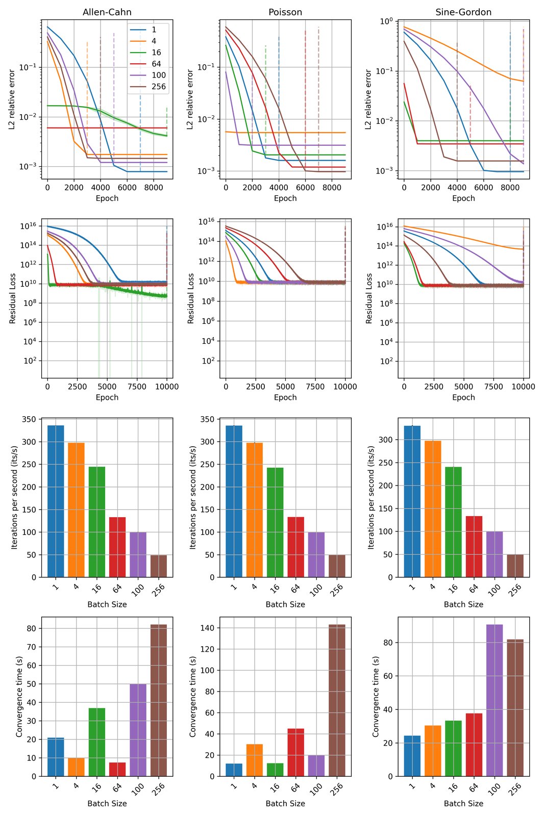
Figure 5: Ablation on randomization batch size with Inseparable and effectively high-dimensional PDEs, dim=100k, 5 runs with different random seeds. Model converges when the difference of L2 error is below 1e-7.
图 5:在不可分且实质高维 PDE上对随机化批大小的消融,维数=100k,5 个不同随机种子。当 L2 误差差低于 1e-7 时视为收敛。