Stacked Attention Networks for Image Question Answering
This CVPR paper is the Open Access version, provided by the Computer Vision Foundation.
Except for this watermark, it is identical to the version available on IEEE Xplore.
Stacked Attention Networks for Image Question Answering
Abstract
This paper presents stacked attention networks (SANs) that learn to answer natural language questions from images. SANs use semantic representation of a question as query to search for the regions in an image that are related to the answer. We argue that image question answering (QA) often requires multiple steps of reasoning. Thus, we develop a multiple-layer SAN in which we query an image multiple times to infer the answer progressively. Experiments conducted on four image QA data sets demonstrate that the proposed SANs significantly outperform previous state-of-the-art approaches. The visualization of the attention layers illustrates the progress that the SAN locates the relevant visual clues that lead to the answer of the question layer-by-layer.
本文提出堆叠注意力网络(SAN),用来根据图像回答自然语言问题。SAN 把问题的语义表示当作查询,在图像中搜索与答案相关的区域。我们认为,图像问答(QA)往往需要多步推理。因此,我们设计了多层 SAN,对同一张图像多次查询,逐步推出答案。在四个图像问答数据集上的实验表明,所提出的 SAN 明显超过此前最好方法。对注意力层的可视化说明了 SAN 如何一层一层地定位通向问题答案的相关视觉线索。
1. Introduction
With the recent advancement in computer vision and in natural language processing (NLP), image question answering (QA) becomes one of the most active research areas [7, 21, 18, 1, 19]. Unlike pure language based QA systems that have been studied extensively in the NLP community [28, 14, 4, 31, 3, 32], image QA systems are designed to automatically answer natural language questions according to the content of a reference image.
随着计算机视觉和自然语言处理(NLP)的近期进展,图像问答(QA)成为最活跃的研究方向之一 [7, 21, 18, 1, 19]。与 NLP 社区已经充分研究过的纯语言问答系统 [28, 14, 4, 31, 3, 32] 不同,图像问答系统的目标是根据参考图像的内容,自动回答自然语言问题。
Most of the recently proposed image QA models are based on neural networks [7, 21, 18, 1, 19]. A commonly used approach was to extract a global image feature vector using a convolution neural network (CNN) [15] and encode the corresponding question as a feature vector using a long short-term memory network (LSTM) [9] and then combine them to infer the answer. Though impressive results have been reported, these models often fail to give precise answers when such answers are related to a set of fine-grained regions in an image.
近来提出的大多数图像问答模型都基于神经网络 [7, 21, 18, 1, 19]。一种常用做法是用卷积神经网络(CNN)[15] 提取一个全局图像特征向量,用长短期记忆网络(LSTM)[9] 把对应问题编码成特征向量,再把两者结合起来推断答案。尽管已经报告了不错的结果,但当答案与图像中一组细粒度区域有关时,这些模型往往给不出精确答案。
By examining the image QA data sets, we find that it is often that case that answering a question from an image requires multi-step reasoning. Take the question and image in Fig. 1 as an example. There are several objects in the image: bicycles, window, street, baskets and dogs. To answer the question what are sitting in the basket on a bicycle, we need to first locate those objects (e.g. basket, bicycle) and concepts (e.g., sitting in) referred in the question, then gradually rule out irrelevant objects, and finally pinpoint to the region that are most indicative to infer the answer (i.e., dogs in the example).
通过考察图像问答数据集,我们发现,根据图像回答问题往往需要多步推理。以图 1 中的问题和图像为例。图中有多个物体:bicycles、window、street、baskets 和 dogs。要回答 what are sitting in the basket on a bicycle 这一问题,需要先定位问题中提到的那些物体(例如 basket、bicycle)和概念(例如 sitting in),再逐步排除无关物体,最后落到对推断答案最有指示作用的区域(在这个例子里就是 dogs)。
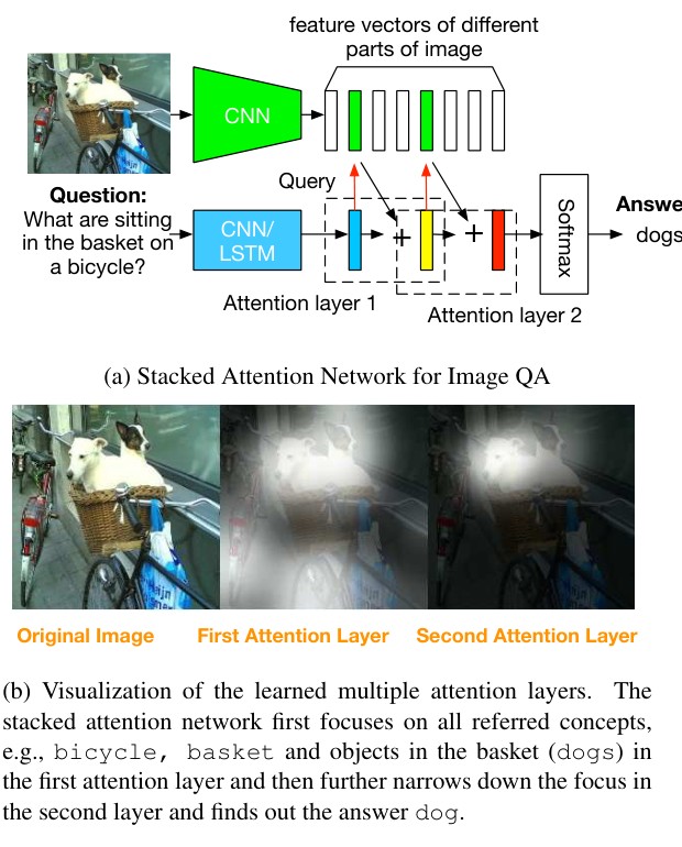
Figure 1: Model architecture and visualization
图 1:模型结构与可视化
In this paper, we propose stacked attention networks (SANs) that allow multi-step reasoning for image QA. SANs can be viewed as an extension of the attention mechanism that has been successfully applied in image captioning [30] and machine translation [2]. The overall architecture of SAN is illustrated in Fig. 1a. The SAN consists of three major components: (1) the image model, which uses a CNN to extract high level image representations, e.g. one vector for each region of the image; (2) the question model, which uses a CNN or a LSTM to extract a semantic vector of the question and (3) the stacked attention model, which locates, via multi-step reasoning, the image regions that are relevant to the question for answer prediction. As illustrated in Fig. 1a, the SAN first uses the question vector to query the image vectors in the first visual attention layer, then combine the question vector and the retrieved image vectors to form a refined query vector to query the image vectors again in the second attention layer. The higher-level attention layer gives a sharper attention distribution focusing on the regions that are more relevant to the answer. Finally, we combine the image features from the highest attention layer with the last query vector to predict the answer.
本文提出堆叠注意力网络(SAN),使图像问答能够进行多步推理。SAN 可以看作是注意力机制的一种扩展,该机制已在图像描述 [30] 和机器翻译 [2] 中得到成功应用。SAN 的总体结构见图 1a。SAN 由三个主要部分组成:(1) 图像模型,用 CNN 提取高层图像表示,例如图像每个区域一个向量;(2) 问题模型,用 CNN 或 LSTM 提取问题的语义向量;(3) 堆叠注意力模型,通过多步推理定位与问题相关的图像区域,用于预测答案。如图 1a 所示,SAN 首先在第一层视觉注意力中用问题向量查询图像向量,再把问题向量与检索到的图像向量结合起来,形成更精细的查询向量,在第二层注意力中再次查询图像向量。更高层的注意力会给出更锐利的注意力分布,聚焦于与答案更相关的区域。最后,我们把最高注意力层的图像特征与最后的查询向量结合起来,预测答案。
The main contributions of our work are three-fold. First, we propose a stacked attention network for image QA tasks. Second, we perform comprehensive evaluations on four image QA benchmarks, demonstrating that the proposed multiple-layer SAN outperforms previous state-of-the-art approaches by a substantial margin. Third, we perform a detailed analysis where we visualize the outputs of different attention layers of the SAN and demonstrate the process that the SAN takes multiple steps to progressively focus the attention on the relevant visual clues that lead to the answer.
本文的主要贡献有三点。第一,我们为图像问答任务提出了堆叠注意力网络。第二,我们在四个图像问答基准上做了全面评测,表明所提出的多层 SAN 以较大幅度超过此前最好方法。第三,我们做了细致分析:可视化 SAN 不同注意力层的输出,并展示 SAN 如何通过多步,逐步把注意力集中到通向答案的相关视觉线索上。
2. Related Work
Image QA is closely related to image captioning [5, 30, 6, 27, 12, 10, 20]. In [27], the system first extracted a high level image feature vector from GoogleNet and then fed it into a LSTM to generate captions. The method proposed in [30] went one step further to use an attention mechanism in the caption generation process. Different from [30, 27], the approach proposed in [6] first used a CNN to detect words given the images, then used a maximum entropy language model to generate a list of caption candidates, and finally used a deep multimodal similarity model (DMSM) to re-rank the candidates. Instead of using a RNN or a LSTM, the DMSM uses a CNN to model the semantics of captions.
图像问答与图像描述密切相关 [5, 30, 6, 27, 12, 10, 20]。在 [27] 中,系统先从 GoogleNet 提取一个高层图像特征向量,再把它送入 LSTM 生成描述。[30] 提出的方法更进一步,在描述生成过程中使用了注意力机制。与 [30, 27] 不同,[6] 提出的方法先用 CNN 根据图像检测词语,再用最大熵语言模型生成一组描述候选,最后用深度多模态相似模型(DMSM)对候选重排序。DMSM 不用 RNN 或 LSTM,而是用 CNN 来建模描述的语义。
Unlike image captioning, in image QA, the question is given and the task is to learn the relevant visual and text representation to infer the answer. In order to facilitate the research of image QA, several data sets have been constructed in [19, 21, 7, 1] either through automatic generation based on image caption data or by human labeling of questions and answers given images. Among them, the image QA data set in [21] is generated based on the COCO caption data set. Given a sentence that describes an image, the authors first used a parser to parse the sentence, then replaced the key word in the sentence using question words and the key word became the answer. [7] created an image QA data set through human labeling. The initial version was in Chinese and then was translated to English. [1] also created an image QA data set through human labeling. They collected questions and answers not only for real images, but also for abstract scenes.
与图像描述不同,在图像问答中,问题是给定的,任务是学习相关的视觉和文本表示来推断答案。为推动图像问答研究,[19, 21, 7, 1] 中构建了若干数据集,构建方式要么是基于图像描述数据自动生成,要么是在给定图像后由人工标注问题和答案。其中,[21] 的图像问答数据集是基于 COCO 描述数据集生成的。给定一句描述图像的句子,作者先用句法分析器分析该句,再用疑问词替换句中的关键词,该关键词就成为答案。[7] 通过人工标注创建了一个图像问答数据集。最初版本是中文,随后被翻译成英文。[1] 也通过人工标注创建了一个图像问答数据集。他们不仅为真实图像收集了问题和答案,也为抽象场景做了收集。
Several image QA models were proposed in the literature. [18] used semantic parsers and image segmentation methods to predict answers based on images and questions. [19, 7] both used encoder-decoder framework to generate answers given images and questions. They first used a LSTM to encoder the images and questions and then used another LSTM to decode the answers. They both fed the image feature to every LSTM cell. [21] proposed several neural network based models, including the encoder-decoder based models that use single direction LSTMs and bi-direction LSTMs, respectively. However, the authors found the concatenation of image features and bag of words features worked the best. [1] first encoded questions with LSTMs and then combined question vectors with image vectors by element wise multiplication. [17] used a CNN for question modeling and used convolution operations to combine question vectors and image feature vectors. We compare the SAN with these models in Sec. 4.
文献中已提出若干图像问答模型。[18] 使用语义分析器和图像分割方法,根据图像和问题预测答案。[19, 7] 都使用编码器-解码器框架,在给定图像和问题后生成答案。他们先用一个 LSTM 对图像和问题编码,再用另一个 LSTM 解码答案。两者都把图像特征送入每一个 LSTM 单元。[21] 提出了若干基于神经网络的模型,包括分别使用单向 LSTM 和双向 LSTM 的编码器-解码器模型。不过,作者发现把图像特征与词袋特征拼接的效果最好。[1] 先用 LSTM 对问题编码,再通过逐元素乘法把问题向量与图像向量结合。[17] 用 CNN 做问题建模,并用卷积运算结合问题向量和图像特征向量。我们将在第 4 节把 SAN 与这些模型进行比较。
To the best of our knowledge, the attention mechanism, which has been proved very successful in image captioning, has not been explored for image QA. The SAN adapt the attention mechanism to image QA, and can be viewed as a significant extension to previous models [30] in that multiple attention layers are used to support multi-step reasoning for the image QA task.
据我们所知,在图像描述中已被证明非常成功的注意力机制,尚未被用于图像问答。SAN 把注意力机制改用于图像问答,并且可以看作对以往模型 [30] 的重要扩展,因为它使用多层注意力来支持图像问答任务中的多步推理。
3. Stacked Attention Networks (SANs)
The overall architecture of the SAN is shown in Fig. 1a. We describe the three major components of SAN in this section: the image model, the question model, and the stacked attention model.
SAN 的总体结构见图 1a。本节描述 SAN 的三个主要组成部分:图像模型、问题模型和堆叠注意力模型。
3.1. Image Model
The image model uses a CNN [13, 23, 26] to get the representation of images. Specifically, the VGGNet [23] is used to extract the image feature map from a raw image :
图像模型用 CNN [13, 23, 26] 得到图像的表示。具体而言,使用 VGGNet [23] 从原始图像 中提取图像特征图 :
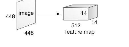
Figure 2: CNN based image model
图 2:基于 CNN 的图像模型
Unlike previous studies [21, 17, 7] that use features from the last inner product layer, we use the features from the last pooling layer, which retains spatial information of the original images. We first rescale the images to be pixels, and then take the features from the last pooling layer, which therefore have a dimension of , as shown in Fig. 2. is the number of regions in the image and 512 is the dimension of the feature vector for each region. Accordingly, each feature vector in corresponds to a pixel region of the input images. We denote by the feature vector of each image region.
与以往使用最后一层内积层特征的研究 [21, 17, 7] 不同,我们使用最后一层池化层的特征 ,从而保留原图的空间信息。我们先把图像缩放到 像素,再取最后一层池化层的特征,因此其维度为 ,如图 2 所示。 是图像中的区域数,512 是每个区域特征向量的维数。相应地, 中的每个特征向量对应输入图像中一块 像素的区域。我们把每个图像区域的特征向量记为 。
Then for modeling convenience, we use a single layer perceptron to transform each feature vector to a new vector that has the same dimension as the question vector (described in Sec. 3.2):
随后,为建模方便,我们用单层感知机把每个特征向量变换到与问题向量相同的维数(见第 3.2 节):
where is a matrix and its i-th column is the visual feature vector for the region indexed by .
其中 是一个矩阵,其第 列 是索引为 的区域的视觉特征向量。
3.2. Question Model
As [25, 22, 6] show that LSTMs and CNNs are powerful to capture the semantic meaning of texts, we explore both models for question representations in this study.
正如 [25, 22, 6] 所示,LSTM 和 CNN 都能有力地捕捉文本的语义,因此本研究对两种问题表示模型都做了考察。
3.2.1 LSTM based question model
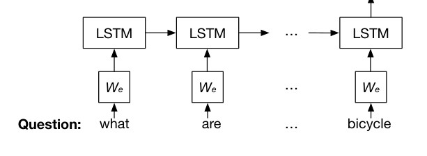
Figure 3: LSTM based question model
图 3:基于 LSTM 的问题模型
The essential structure of a LSTM unit is a memory cell which reserves the state of a sequence. At each step, the LSTM unit takes one input vector (word vector in our case) and updates the memory cell , then output a hidden state . The update process uses the gate mechanism. A forget gate controls how much information from past state is preserved. An input gate controls how much the current input updates the memory cell. An output gate controls how much information of the memory is fed to the output as hidden state. The detailed update process is as follows:
LSTM 单元的核心结构是记忆细胞 ,它保存序列的状态。在每一步,LSTM 单元接收一个输入向量(在我们这里是词向量),更新记忆细胞 ,再输出隐状态 。更新过程使用门机制。遗忘门 控制保留多少来自过去状态 的信息。输入门 控制当前输入 在多大程度上更新记忆细胞。输出门 控制把多少记忆信息作为隐状态送到输出。具体更新过程如下:
where are input gate, forget gate, output gate and memory cell, respectively. The weight matrix and bias are parameters of the LSTM and are learned on training data.
其中 分别是输入门、遗忘门、输出门和记忆细胞。权重矩阵和偏置是 LSTM 的参数,在训练数据上学习。
Given the question , where is the one hot vector representation of word at position , we first embed the words to a vector space through an embedding matrix . Then for every time step, we feed the embedding vector of words in the question to LSTM:
给定问题 ,其中 是位置 处词的 one-hot 向量表示,我们先通过嵌入矩阵把词嵌入到向量空间:。随后在每个时间步,把问题中词的嵌入向量送入 LSTM:
As shown in Fig. 3, the question what are sitting in the basket on a bicycle is fed into the LSTM. Then the final hidden layer is taken as the representation vector for the question, i.e., .
如图 3 所示,问题 what are sitting in the basket on a bicycle 被送入 LSTM。然后取最后的隐层作为问题的表示向量,即 。
3.2.2 CNN based question model
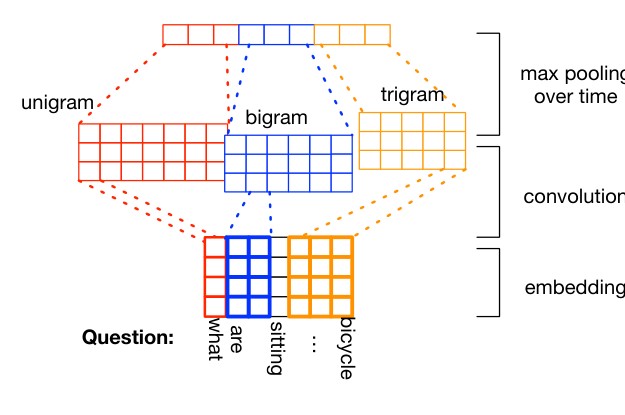
Figure 4: CNN based question model
图 4:基于 CNN 的问题模型
In this study, we also explore to use a CNN similar to [11] for question representation. Similar to the LSTM-based question model, we first embed words to vectors and get the question vector by concatenating the word vectors:
本研究中,我们也探索使用与 [11] 类似的 CNN 来做问题表示。与基于 LSTM 的问题模型类似,我们先把词嵌入为向量 ,再通过拼接词向量得到问题向量:
Then we apply convolution operation on the word embedding vectors. We use three convolution filters, which have the size of one (unigram), two (bigram) and three (trigram) respectively. The -th convolution output using window size is given by:
然后我们对词嵌入向量做卷积运算。我们使用三种卷积滤波器,窗口大小分别为 1(unigram)、2(bigram)和 3(trigram)。使用窗口大小 时,第 个卷积输出为:
The filter is applied only to window of size . is the convolution weight and is the bias. The feature map of the filter with convolution size is given by:
该滤波器只作用于大小为 的窗口 。 是卷积权重, 是偏置。卷积大小为 的滤波器的特征图为:
Then we apply max-pooling over the feature maps of the convolution size and denote it as
然后我们对卷积大小为 的特征图做最大池化,并记为
The max-pooling over these vectors is a coordinate-wise max operation. For convolution feature maps of different sizes , we concatenate them to form the feature representation vector of the whole question sentence:
对这些向量的最大池化是按坐标取最大。对于不同大小 的卷积特征图,我们把它们拼接起来,形成整个问句的特征表示向量:
hence is the CNN based question vector.
因此 就是基于 CNN 的问题向量。
The diagram of CNN model for question is shown in Fig. 4. The convolutional and pooling layers for unigrams, bigrams and trigrams are drawn in red, blue and orange, respectively.
问题 CNN 模型的示意图见图 4。unigram、bigram 和 trigram 的卷积层与池化层分别用红、蓝、橙色画出。
3.3. Stacked Attention Networks
Given the image feature matrix and the question feature vector , SAN predicts the answer via multi-step reasoning.
给定图像特征矩阵 和问题特征向量 ,SAN 通过多步推理来预测答案。
In many cases, an answer only related to a small region of an image. For example, in Fig. 1b, although there are multiple objects in the image: bicycles, baskets, window, street and dogs and the answer to the question only relates to dogs. Therefore, using the one global image feature vector to predict the answer could lead to suboptimal results due to the noises introduced from regions that are irrelevant to the potential answer. Instead, reasoning via multiple attention layers progressively, the SAN are able to gradually filter out noises and pinpoint the regions that are highly relevant to the answer.
在许多情况下,答案只与图像中一块很小的区域有关。例如在图 1b 中,尽管图像里有多个物体:bicycles、baskets、window、street 和 dogs,而问题的答案只与 dogs 有关。因此,用一个全局图像特征向量来预测答案,可能因与潜在答案无关的区域引入噪声,而导致次优结果。相反,通过多层注意力逐步推理,SAN 能够逐渐滤除噪声,并定位到与答案高度相关的区域。
Given the image feature matrix and the question vector , we first feed them through a single layer neural network and then a softmax function to generate the attention distribution over the regions of the image:
给定图像特征矩阵 和问题向量 ,我们先把它们送入单层神经网络,再用 softmax 函数生成图像各区域上的注意力分布:
where , is the image representation dimension and is the number of image regions, is a dimensional vector. Suppose and , then is an dimensional vector, which corresponds to the attention probability of each image region given . Note that we denote by the addition of a matrix and a vector. Since and both are vectors, the addition between a matrix and a vector is performed by adding each column of the matrix by the vector.
其中 , 是图像表示的维数, 是图像区域数, 是 维向量。设 且 ,则 是一个 维向量,对应给定 时每个图像区域的注意力概率。注意,我们用 表示矩阵与向量的加法。由于 ,而 都是向量,矩阵与向量相加的做法是把向量加到矩阵的每一列上。
Based on the attention distribution, we calculate the weighted sum of the image vectors, each from a region, as in Eq. 17. We then combine with the question vector to form a refined query vector as in Eq. 18. is regarded as a refined query since it encodes both question information and the visual information that is relevant to the potential answer:
根据注意力分布,我们按 (17) 式计算各区域图像向量的加权和 。再按 (18) 式把 与问题向量 结合起来,形成更精细的查询向量 。之所以把 看作更精细的查询,是因为它同时编码了问题信息,以及与潜在答案相关的视觉信息:
Compared to models that simply combine the question vector and the global image vector, attention models construct a more informative since higher weights are put on the visual regions that are more relevant to the question. However, for complicated questions, a single attention layer is not sufficient to locate the correct region for answer prediction. For example, the question in Fig. 1 what are sitting in the basket on a bicycle refers to some subtle relationships among multiple objects in an image. Therefore, we iterate the above query-attention process using multiple attention layers, each extracting more fine-grained visual attention information for answer prediction. Formally, the SANs take the following formula: for the -th attention layer, we compute:
与只是简单结合问题向量和全局图像向量的模型相比,注意力模型构造出的 信息更丰富,因为与问题更相关的视觉区域会得到更高的权重。不过,对于复杂问题,单层注意力不足以定位到预测答案所需的正确区域。例如,图 1 中的问题 what are sitting in the basket on a bicycle 涉及图像中多个物体之间较为细微的关系。因此,我们用多层注意力迭代上述查询-注意力过程,每一层都为预测答案提取更细粒度的视觉注意力信息。形式上,SAN 采用如下公式:对第 层注意力,我们计算:
where is initialized to be . Then the aggregated image feature vector is added to the previous query vector to form a new query vector:
其中 初始化为 。然后把聚合后的图像特征向量加到前一查询向量上,形成新的查询向量:
That is, in every layer, we use the combined question and image vector as the query for the image. After the image region is picked, we update the new query vector as . We repeat this times and then use the final to infer the answer:
也就是说,在每一层,我们都用结合后的问题与图像向量 作为对图像的查询。选定图像区域后,把新的查询向量更新为 。我们将此重复 次,再用最后的 推断答案:
Fig. 1b illustrates the reasoning process by an example. In the first attention layer, the model identifies roughly the area that are relevant to basket, bicycle, and sitting in. In the second attention layer, the model focuses more sharply on the region that corresponds to the answer dogs. More examples can be found in Sec. 4.
图 1b 用一个例子说明了推理过程。在第一层注意力中,模型大致识别出与 basket、bicycle 和 sitting in 相关的区域。在第二层注意力中,模型更锐利地聚焦于对应答案 dogs 的区域。更多例子见第 4 节。
4. Experiments
4.1. Data sets
We evaluate the SAN on four image QA data sets. DAQUAR-ALL is proposed in [18]. There are 6,795 training questions and 5,673 test questions. These questions are generated on 795 and 654 images respectively. The images are mainly indoor scenes. The questions are categorized into three types including Object, Color and Number. Most of the answers are single words. Following the setting in [21, 17, 19], we exclude data samples that have multiple words answers. The remaining data set covers 90% of the original data set.
我们在四个图像问答数据集上评估 SAN。DAQUAR-ALL 由 [18] 提出。其中有 6,795 个训练问题和 5,673 个测试问题。这些问题分别在 795 张和 654 张图像上生成。图像以室内场景为主。问题被分成 Object、Color 和 Number 三类。大多数答案是单个词。沿用 [21, 17, 19] 中的设置,我们排除答案为多个词的样本。剩余数据占原数据集的 90%。
DAQUAR-REDUCED is a reduced version of DAQUAR-ALL. There are 3,876 training samples and 297 test samples. This data set is constrained to 37 object categories and uses only 25 test images. The single word answers data set covers 98% of the original data set.
DAQUAR-REDUCED 是 DAQUAR-ALL 的缩减版本。其中有 3,876 个训练样本和 297 个测试样本。该数据集被限制在 37 个物体类别,并且只使用 25 张测试图像。单词语答案的数据占原数据集的 98%。
COCO-QA is proposed in [21]. Based on the Microsoft COCO data set, the authors first parse the caption of the image with an off-the-shelf parser, then replace the key components in the caption with question words for form questions. There are 78,736 training samples and 38,948 test samples in the data set. These questions are based on 8,000 and 4,000 images respectively. There are four types of questions including Object, Number, Color, and Location. Each type takes 70%, 7%, 17%, and 6% of the whole data set, respectively. All answers in this data set are single word.
COCO-QA 由 [21] 提出。基于 Microsoft COCO 数据集,作者先用现成的句法分析器分析图像描述,再用疑问词替换描述中的关键成分以构成问题。该数据集中有 78,736 个训练样本和 38,948 个测试样本。这些问题分别基于 8,000 张和 4,000 张图像。问题有四类:Object、Number、Color 和 Location。各类分别占整个数据集的 70%、7%、17% 和 6%。该数据集中的全部答案都是单个词。
VQA is created through human labeling [1]. The data set uses images in the COCO image caption data set [16]. Unlike the other data sets, for each image, there are three questions and for each question, there are ten answers labeled by human annotators. There are 248,349 training questions and 121,512 validation questions in the data set. Following [1], we use the top 1000 most frequent answer as possible outputs and this set of answers covers 82.67% of all answers. We first studied the performance of the proposed model on the validation set. Following [6], we split the validation data set into two halves, val1 and val2. We use training set and val1 to train and validate and val2 to test locally. The results on the val2 set are reported in Table. 6. We also evaluated the best model, SAN(2, CNN), on the standard test server as provided in [1] and report the results in Table. 5.
VQA 通过人工标注创建 [1]。该数据集使用 COCO 图像描述数据集 [16] 中的图像。与其他数据集不同,每张图像有三个问题,每个问题有十个由标注者给出的答案。数据集中有 248,349 个训练问题和 121,512 个验证问题。沿用 [1],我们把出现频率最高的 1000 个答案作为可能输出,这组答案覆盖了全部答案的 82.67%。我们先在验证集上考察了所提出模型的表现。沿用 [6],我们把验证集分成两半,val1 和 val2。用训练集和 val1 做训练与验证,用 val2 做本地测试。val2 上的结果见表 6。我们还在 [1] 提供的标准测试服务器上评估了最好模型 SAN(2, CNN),结果见表 5。
4.2. Baselines and evaluation methods
We compare our models with a set of baselines proposed recently [21, 1, 18, 19, 17] on image QA. Since the results of these baselines are reported on different data sets in different literature, we present the experimental results on different data sets in different tables.
我们在图像问答上,把模型与近来提出的一组基线 [21, 1, 18, 19, 17] 进行比较。由于这些基线的结果是在不同文献、不同数据集上报告的,我们把不同数据集上的实验结果分表给出。
For all four data sets, we formulate image QA as a classification problem since most of answers are single words. We evaluate the model using classification accuracy as reported in [1, 21, 19]. The reference models also report the Wu-Palmer similarity (WUPS) measure [29]. The WUPS measure calculates the similarity between two words based on their longest common subsequence in the taxonomy tree. We can set a threshold for WUPS, if the similarity is less than the threshold, then it is zeroed out. Following the reference models, we use WUPS0.9 and WUPS0.0 as evaluation metrics besides the classification accuracy. The evaluation on the VQA data set is different from other three data sets, since for each question there are ten answer labels that may or may not be the same. We follow [1] to use the following metric: human labels that match that answer, which basically gives full credit to the answer when three or more of the ten human labels match the answer and gives partial credit if there are less matches.
对全部四个数据集,由于大多数答案是单个词,我们把图像问答表述为分类问题。我们按 [1, 21, 19] 所报告的方式,用分类准确率评估模型。对照模型还报告了 Wu-Palmer 相似度(WUPS)指标 [29]。WUPS 根据两个词在分类树上的最长公共子序列来计算相似度。我们可以为 WUPS 设定一个阈值,若相似度低于该阈值,则记为零。沿用对照模型,除分类准确率外,我们还使用 WUPS0.9 和 WUPS0.0 作为评价指标。VQA 数据集上的评价与其他三个数据集不同,因为每个问题有十个答案标签,这些标签可能相同也可能不同。我们沿用 [1] 使用如下指标: 与该答案匹配的人工标签数 ,其基本含义是:当十个人工标签中有三个或更多与该答案匹配时,给满分;匹配更少时给部分分数。
4.3. Model configuration and training
For the image model, we use the VGGNet to extract features. When training the SAN, the parameter set of the CNN of the VGGNet is fixed. We take the output from the last pooling layer as our image feature which has a dimension of .
对图像模型,我们用 VGGNet 提取特征。训练 SAN 时,VGGNet 中 CNN 的参数保持固定。我们取最后一层池化层的输出作为图像特征,其维度为 。
For DAQUAR and COCO-QA, we set the word embedding dimension and LSTM’s dimension to be 500 in the question model. For the CNN based question model, we set the unigram, bigram and trigram convolution filter size to be 128, 256, 256 respectively. The combination of these filters makes the question vector size to be 640. For VQA dataset, since it is larger than other data sets, we double the model size of the LSTM and the CNN to accommodate the large data set and the large number of classes. In evaluation, we experiment with SAN with one and two attention layers. We find that using three or more attention layers does not further improve the performance.
对 DAQUAR 和 COCO-QA,我们在问题模型中把词嵌入维数和 LSTM 维数设为 500。对基于 CNN 的问题模型,我们把 unigram、bigram 和 trigram 卷积滤波器的大小分别设为 128、256、256。这些滤波器组合后,问题向量的大小为 640。对 VQA 数据集,由于它比其他数据集更大,我们把 LSTM 和 CNN 的模型规模加倍,以适应较大的数据集和较多的类别。在评测中,我们实验了带一层和两层注意力的 SAN。我们发现,使用三层或更多注意力层并不能进一步提高表现。
In our experiments, all the models are trained using stochastic gradient descent with momentum 0.9. The batch size is fixed to be 100. The best learning rate is picked using grid search. Gradient clipping technique [8] and dropout [24] are used.
在我们的实验中,全部模型都使用动量为 0.9 的随机梯度下降来训练。批量大小固定为 100。最佳学习率通过网格搜索选取。使用了梯度裁剪技术 [8] 和 dropout [24]。
Our code is publicly available at https://github.com/zcyang/imageqa-san
我们的代码公开发布于 https://github.com/zcyang/imageqa-san
4.4. Results and analysis
The experimental results on DAQUAR-ALL, DAQUAR-REDUCED, COCO-QA and VQA are presented in Table. 1 to 6 respectively. Our model names explain their settings: SAN is short for the proposed stacked attention networks, the value 1 or 2 in the brackets refer to using one or two attention layers, respectively. The keyword LSTM or CNN refers to the question model that SANs use.
DAQUAR-ALL、DAQUAR-REDUCED、COCO-QA 和 VQA 上的实验结果分别见表 1 至表 6。我们的模型名称说明了其设置:SAN 是所提出的堆叠注意力网络的简称,括号中的 1 或 2 分别表示使用一层或两层注意力。关键词 LSTM 或 CNN 表示 SAN 所使用的问题模型。
Table 1: DAQUAR-ALL results, in percentage
| Methods | Accuracy | WUPS0.9 | WUPS0.0 |
|---|---|---|---|
| Multi-World: [18] | |||
| Multi-World | 7.9 | 11.9 | 38.8 |
| Ask-Your-Neurons: [19] | |||
| Language | 19.1 | 25.2 | 65.1 |
| Language + IMG | 21.7 | 28.0 | 65.0 |
| CNN: [17] | |||
| IMG-CNN | 23.4 | 29.6 | 63.0 |
| Ours: | |||
| SAN(1, LSTM) | 28.9 | 34.7 | 68.5 |
| SAN(1, CNN) | 29.2 | 35.1 | 67.8 |
| SAN(2, LSTM) | 29.3 | 34.9 | 68.1 |
| SAN(2, CNN) | 29.3 | 35.1 | 68.6 |
| Human :[18] | |||
| Human | 50.2 | 50.8 | 67.3 |
表 1:DAQUAR-ALL 结果,单位为百分比
| 方法 | 准确率 | WUPS0.9 | WUPS0.0 |
|---|---|---|---|
| Multi-World: [18] | |||
| Multi-World | 7.9 | 11.9 | 38.8 |
| Ask-Your-Neurons: [19] | |||
| Language | 19.1 | 25.2 | 65.1 |
| Language + IMG | 21.7 | 28.0 | 65.0 |
| CNN: [17] | |||
| IMG-CNN | 23.4 | 29.6 | 63.0 |
| 本文: | |||
| SAN(1, LSTM) | 28.9 | 34.7 | 68.5 |
| SAN(1, CNN) | 29.2 | 35.1 | 67.8 |
| SAN(2, LSTM) | 29.3 | 34.9 | 68.1 |
| SAN(2, CNN) | 29.3 | 35.1 | 68.6 |
| Human :[18] | |||
| Human | 50.2 | 50.8 | 67.3 |
The experimental results in Table. 1 to 6 show that the two-layer SAN gives the best results across all data sets and the two kinds of question models in the SAN, LSTM and CNN, give similar performance. For example, on DAQUAR-ALL (Table. 1), both of the proposed two-layer SANs outperform the two best baselines, the IMG-CNN in [17] and the Ask-Your-Neurons in [19], by 5.9% and 7.6% absolute in accuracy, respectively. Similar range of improvements are observed in metrics of WUPS0.9 and WUPS0.0.
表 1 至表 6 中的实验结果表明,两层 SAN 在全部数据集上都给出最好结果,并且 SAN 中的两种问题模型 LSTM 和 CNN 表现相近。例如,在 DAQUAR-ALL(表 1)上,所提出的两个两层 SAN 都超过了两个最好基线,即 [17] 中的 IMG-CNN 和 [19] 中的 Ask-Your-Neurons,准确率分别绝对提高 5.9% 和 7.6%。在 WUPS0.9 和 WUPS0.0 指标上也观察到相似幅度的提升。
Table 2: DAQUAR-REDUCED results, in percentage
| Methods | Accuracy | WUPS0.9 | WUPS0.0 |
|---|---|---|---|
| Multi-World: [18] | |||
| Multi-World | 12.7 | 18.2 | 51.5 |
| Ask-Your-Neurons: [19] | |||
| Language | 31.7 | 38.4 | 80.1 |
| Language + IMG | 34.7 | 40.8 | 79.5 |
| VSE: [21] | |||
| GUESS | 18.2 | 29.7 | 77.6 |
| BOW | 32.7 | 43.2 | 81.3 |
| LSTM | 32.7 | 43.5 | 81.6 |
| IMG+BOW | 34.2 | 45.0 | 81.5 |
| VIS+LSTM | 34.4 | 46.1 | 82.2 |
| 2-VIS+BLSTM | 35.8 | 46.8 | 82.2 |
| CNN: [17] | |||
| IMG-CNN | 39.7 | 44.9 | 83.1 |
| Ours: | |||
| SAN(1, LSTM) | 45.2 | 49.6 | 84.0 |
| SAN(1, CNN) | 45.2 | 49.6 | 83.7 |
| SAN(2, LSTM) | 46.2 | 51.2 | 85.1 |
| SAN(2, CNN) | 45.5 | 50.2 | 83.6 |
| Human :[18] | |||
| Human | 60.3 | 61.0 | 79.0 |
表 2:DAQUAR-REDUCED 结果,单位为百分比
| 方法 | 准确率 | WUPS0.9 | WUPS0.0 |
|---|---|---|---|
| Multi-World: [18] | |||
| Multi-World | 12.7 | 18.2 | 51.5 |
| Ask-Your-Neurons: [19] | |||
| Language | 31.7 | 38.4 | 80.1 |
| Language + IMG | 34.7 | 40.8 | 79.5 |
| VSE: [21] | |||
| GUESS | 18.2 | 29.7 | 77.6 |
| BOW | 32.7 | 43.2 | 81.3 |
| LSTM | 32.7 | 43.5 | 81.6 |
| IMG+BOW | 34.2 | 45.0 | 81.5 |
| VIS+LSTM | 34.4 | 46.1 | 82.2 |
| 2-VIS+BLSTM | 35.8 | 46.8 | 82.2 |
| CNN: [17] | |||
| IMG-CNN | 39.7 | 44.9 | 83.1 |
| 本文: | |||
| SAN(1, LSTM) | 45.2 | 49.6 | 84.0 |
| SAN(1, CNN) | 45.2 | 49.6 | 83.7 |
| SAN(2, LSTM) | 46.2 | 51.2 | 85.1 |
| SAN(2, CNN) | 45.5 | 50.2 | 83.6 |
| Human :[18] | |||
| Human | 60.3 | 61.0 | 79.0 |
We also observe significant improvements on DAQUAR-REDUCED (Table. 2), i.e., our SAN(2, LSTM) outperforms the IMG-CNN [17], the 2-VIS+BLSTM [21], the Ask-Your-Neurons approach [19] and the Multi-World [18] by 6.5%, 10.4%, 11.5% and 33.5% absolute in accuracy, respectively. On the larger COCO-QA data set, the proposed two-layer SANs significantly outperform the best baselines from [17] (IMG-CNN) and [21] (IMG+BOW and 2-VIS+BLSTM) by 5.1% and 6.6% in accuracy (Table. 3). Table. 5 summarizes the performance of various models on VQA, which is the largest among the four data sets. The overall results show that our best model, SAN(2, CNN), outperforms the LSTM Q+I model, the best baseline from [1], by 4.8% absolute. The superior performance of the SANs across all four benchmarks demonstrate the effectiveness of using multiple layers of attention.
我们在 DAQUAR-REDUCED(表 2)上也观察到明显提升,即我们的 SAN(2, LSTM) 分别比 IMG-CNN [17]、2-VIS+BLSTM [21]、Ask-Your-Neurons 方法 [19] 和 Multi-World [18] 在准确率上绝对高出 6.5%、10.4%、11.5% 和 33.5%。在更大的 COCO-QA 数据集上,所提出的两层 SAN 明显超过 [17] 的最好基线(IMG-CNN)以及 [21] 的最好基线(IMG+BOW 和 2-VIS+BLSTM),准确率分别高出 5.1% 和 6.6%(表 3)。表 5 汇总了各模型在四个数据集中最大的 VQA 上的表现。总体结果表明,我们最好的模型 SAN(2, CNN) 比 [1] 中最好的基线 LSTM Q+I 绝对高出 4.8%。SAN 在全部四个基准上的优异表现,说明了使用多层注意力的有效性。
Table 3: COCO-QA results, in percentage
| Methods | Accuracy | WUPS0.9 | WUPS0.0 |
|---|---|---|---|
| VSE: [21] | |||
| GUESS | 6.7 | 17.4 | 73.4 |
| BOW | 37.5 | 48.5 | 82.8 |
| LSTM | 36.8 | 47.6 | 82.3 |
| IMG | 43.0 | 58.6 | 85.9 |
| IMG+BOW | 55.9 | 66.8 | 89.0 |
| VIS+LSTM | 53.3 | 63.9 | 88.3 |
| 2-VIS+BLSTM | 55.1 | 65.3 | 88.6 |
| CNN: [17] | |||
| IMG-CNN | 55.0 | 65.4 | 88.6 |
| CNN | 32.7 | 44.3 | 80.9 |
| Ours: | |||
| SAN(1, LSTM) | 59.6 | 69.6 | 90.1 |
| SAN(1, CNN) | 60.7 | 70.6 | 90.5 |
| SAN(2, LSTM) | 61.0 | 71.0 | 90.7 |
| SAN(2, CNN) | 61.6 | 71.6 | 90.9 |
表 3:COCO-QA 结果,单位为百分比
| 方法 | 准确率 | WUPS0.9 | WUPS0.0 |
|---|---|---|---|
| VSE: [21] | |||
| GUESS | 6.7 | 17.4 | 73.4 |
| BOW | 37.5 | 48.5 | 82.8 |
| LSTM | 36.8 | 47.6 | 82.3 |
| IMG | 43.0 | 58.6 | 85.9 |
| IMG+BOW | 55.9 | 66.8 | 89.0 |
| VIS+LSTM | 53.3 | 63.9 | 88.3 |
| 2-VIS+BLSTM | 55.1 | 65.3 | 88.6 |
| CNN: [17] | |||
| IMG-CNN | 55.0 | 65.4 | 88.6 |
| CNN | 32.7 | 44.3 | 80.9 |
| 本文: | |||
| SAN(1, LSTM) | 59.6 | 69.6 | 90.1 |
| SAN(1, CNN) | 60.7 | 70.6 | 90.5 |
| SAN(2, LSTM) | 61.0 | 71.0 | 90.7 |
| SAN(2, CNN) | 61.6 | 71.6 | 90.9 |
Table 4: COCO-QA accuracy per class, in percentage
| Methods | Objects | Number | Color | Location |
|---|---|---|---|---|
| VSE: [21] | ||||
| GUESS | 2.1 | 35.8 | 13.9 | 8.9 |
| BOW | 37.3 | 43.6 | 34.8 | 40.8 |
| LSTM | 35.9 | 45.3 | 36.3 | 38.4 |
| IMG | 40.4 | 29.3 | 42.7 | 44.2 |
| IMG+BOW | 58.7 | 44.1 | 52.0 | 49.4 |
| VIS+LSTM | 56.5 | 46.1 | 45.9 | 45.5 |
| 2-VIS+BLSTM | 58.2 | 44.8 | 49.5 | 47.3 |
| Ours: | ||||
| SAN(1, LSTM) | 62.5 | 49.0 | 54.8 | 51.6 |
| SAN(1, CNN) | 63.6 | 48.7 | 56.7 | 52.7 |
| SAN(2, LSTM) | 63.6 | 49.8 | 57.9 | 52.8 |
| SAN(2, CNN) | 64.5 | 48.6 | 57.9 | 54.0 |
表 4:COCO-QA 各类准确率,单位为百分比
| 方法 | Objects | Number | Color | Location |
|---|---|---|---|---|
| VSE: [21] | ||||
| GUESS | 2.1 | 35.8 | 13.9 | 8.9 |
| BOW | 37.3 | 43.6 | 34.8 | 40.8 |
| LSTM | 35.9 | 45.3 | 36.3 | 38.4 |
| IMG | 40.4 | 29.3 | 42.7 | 44.2 |
| IMG+BOW | 58.7 | 44.1 | 52.0 | 49.4 |
| VIS+LSTM | 56.5 | 46.1 | 45.9 | 45.5 |
| 2-VIS+BLSTM | 58.2 | 44.8 | 49.5 | 47.3 |
| 本文: | ||||
| SAN(1, LSTM) | 62.5 | 49.0 | 54.8 | 51.6 |
| SAN(1, CNN) | 63.6 | 48.7 | 56.7 | 52.7 |
| SAN(2, LSTM) | 63.6 | 49.8 | 57.9 | 52.8 |
| SAN(2, CNN) | 64.5 | 48.6 | 57.9 | 54.0 |
Table 5: VQA results on the official server, in percentage
| Methods | test-dev All | test-dev Yes/No | test-dev Number | test-dev Other | test-std All |
|---|---|---|---|---|---|
| VQA: [1] | |||||
| Question | 48.1 | 75.7 | 36.7 | 27.1 | - |
| Image | 28.1 | 64.0 | 0.4 | 3.8 | - |
| Q+I | 52.6 | 75.6 | 33.7 | 37.4 | - |
| LSTM Q | 48.8 | 78.2 | 35.7 | 26.6 | - |
| LSTM Q+I | 53.7 | 78.9 | 35.2 | 36.4 | 54.1 |
| SAN(2, CNN) | 58.7 | 79.3 | 36.6 | 46.1 | 58.9 |
表 5:在官方服务器上的 VQA 结果,单位为百分比
| 方法 | test-dev All | test-dev Yes/No | test-dev Number | test-dev Other | test-std All |
|---|---|---|---|---|---|
| VQA: [1] | |||||
| Question | 48.1 | 75.7 | 36.7 | 27.1 | - |
| Image | 28.1 | 64.0 | 0.4 | 3.8 | - |
| Q+I | 52.6 | 75.6 | 33.7 | 37.4 | - |
| LSTM Q | 48.8 | 78.2 | 35.7 | 26.6 | - |
| LSTM Q+I | 53.7 | 78.9 | 35.2 | 36.4 | 54.1 |
| SAN(2, CNN) | 58.7 | 79.3 | 36.6 | 46.1 | 58.9 |
Table 6: VQA results on our partition, in percentage
| Methods | All | Yes/No 36% | Number 10% | Other 54% |
|---|---|---|---|---|
| SAN(1, LSTM) | 56.6 | 78.1 | 41.6 | 44.8 |
| SAN(1, CNN) | 56.9 | 78.8 | 42.0 | 45.0 |
| SAN(2, LSTM) | 57.3 | 78.3 | 42.2 | 45.9 |
| SAN(2, CNN) | 57.6 | 78.6 | 41.8 | 46.4 |
表 6:在我们划分的数据上的 VQA 结果,单位为百分比
| 方法 | All | Yes/No 36% | Number 10% | Other 54% |
|---|---|---|---|---|
| SAN(1, LSTM) | 56.6 | 78.1 | 41.6 | 44.8 |
| SAN(1, CNN) | 56.9 | 78.8 | 42.0 | 45.0 |
| SAN(2, LSTM) | 57.3 | 78.3 | 42.2 | 45.9 |
| SAN(2, CNN) | 57.6 | 78.6 | 41.8 | 46.4 |
In order to study the strength and weakness of the SAN in detail, we report performance at the question-type level on the two large data sets, COCO-QA and VQA, in Table. 4 and 5, respectively. We observe that on COCO-QA, compared to the two best baselines, IMG+BOW and 2-VIS+BLSTM, our best model SAN(2, CNN) improves 7.2% in the question type of Object, followed by 6.1% in Location, 5.7% in Color and 4.2% in Number. We observe similar trend of improvements on VQA. As shown in Table. 5, compared to the best baseline LSTM Q+I, the biggest improvement of SAN(2, CNN) is in the Other type, 9.7%, followed by the 1.4% improvement in Number and 0.4% improvement in Yes/No. Note that the Other type in VQA refers to questions that usually have the form of “what color, what kind, what are, what type, where” etc., which are similar to question types of Color, Objects and Location in COCO-QA. The VQA data set has a special Yes/No type of questions. The SAN only improves the performance of this type of questions slightly. This could due to that the answer for a Yes/No question is very question dependent, so better modeling of the visual information does not provide much additional gains. This also confirms the similar observation reported in [1], e.g., using additional image information only slightly improves the performance in Yes/No, as shown in Table. 5, Q+I vs Question, and LSTM Q+I vs LSTM Q.
为了更细致地考察 SAN 的长处和不足,我们在两个较大的数据集 COCO-QA 和 VQA 上,按问题类型报告了表现,分别见表 4 和表 5。我们观察到,在 COCO-QA 上,与两个最好基线 IMG+BOW 和 2-VIS+BLSTM 相比,我们最好的模型 SAN(2, CNN) 在 Object 类问题上提高 7.2%,随后是 Location 提高 6.1%,Color 提高 5.7%,Number 提高 4.2%。在 VQA 上也观察到类似的提升趋势。如表 5 所示,与最好基线 LSTM Q+I 相比,SAN(2, CNN) 提升最大的是 Other 类,为 9.7%,随后是 Number 提高 1.4%,Yes/No 提高 0.4%。需要指出,VQA 中的 Other 类通常是 “what color, what kind, what are, what type, where” 这类问题,与 COCO-QA 中的 Color、Objects 和 Location 类型相近。VQA 数据集还有一类特殊的 Yes/No 问题。SAN 对这类问题的提升很小。这可能是因为 Yes/No 问题的答案非常依赖于问题本身,因此更好地建模视觉信息并不能带来多少额外收益。这也印证了 [1] 中报告的类似观察,例如,如表 5 中 Q+I 对比 Question、以及 LSTM Q+I 对比 LSTM Q 所示,加入额外的图像信息对 Yes/No 的提升也很有限。
Our results demonstrate clearly the positive impact of using multiple attention layers. In all four data sets, two-layer SANs always perform better than the one-layer SAN. Specifically, on COCO-QA, on average the two-layer SANs outperform the one-layer SANs by 2.2% in the type of Color, followed by 1.3% and 1.0% in the Location and Objects categories, and then 0.4% in Number. This aligns to the order of the improvements of the SAN over baselines. Similar trends are observed on VQA (Table. 6), e.g., the two-layer SAN improve over the one-layer SAN by 1.4% for the Other type of question, followed by 0.2% improvement for Number, and flat for Yes/No.
我们的结果清楚地表明,使用多层注意力具有积极作用。在全部四个数据集上,两层 SAN 始终好于一层 SAN。具体而言,在 COCO-QA 上,两层 SAN 平均比一层 SAN 在 Color 类上高出 2.2%,随后是 Location 和 Objects 类分别高出 1.3% 和 1.0%,Number 类高出 0.4%。这与 SAN 相对基线的提升顺序一致。在 VQA(表 6)上也观察到类似趋势,例如两层 SAN 比一层 SAN 在 Other 类问题上提高 1.4%,在 Number 上提高 0.2%,在 Yes/No 上则持平。
4.5. Visualization of attention layers
In this section, we present analysis to demonstrate that using multiple attention layers to perform multi-step reasoning leads to more fine-grained attention layer-by-layer in locating the regions that are relevant to the potential answers. We do so by visualizing the outputs of the attention layers of a sample set of images from the COCO-QA test set. Note the attention probability distribution is of size and the original image is , we up-sample the attention probability distribution and apply a Gaussian filter to make it the same size as the original image.
本节通过分析表明,使用多层注意力做多步推理,可以一层一层地得到更细粒度的注意力,从而定位到与潜在答案相关的区域。我们的做法是,可视化 COCO-QA 测试集中一组样本图像的注意力层输出。注意,注意力概率分布的大小为 ,原图为 ,我们把注意力概率分布上采样,并施加高斯滤波,使其与原图尺寸相同。
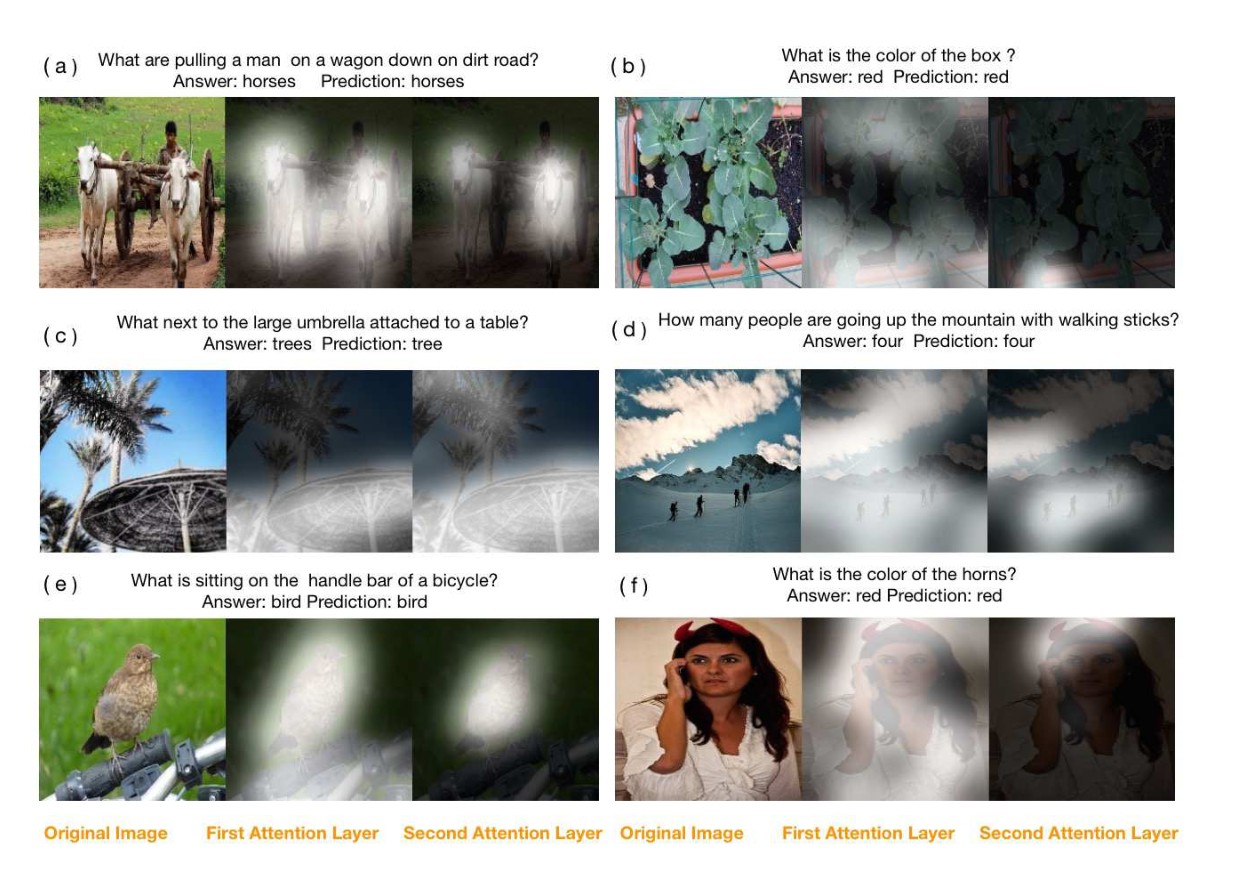
Figure 5: Visualization of two attention layers
图 5:两层注意力的可视化
Fig. 5 presents six examples. More examples are presented in the appendix. They cover types as broad as Object, Numbers, Color and Location. For each example, the three images from left to right are the original image, the output of the first attention layer and the output of the second attention layer, respectively. The bright part of the image is the detected attention. Across all those examples, we see that in the first attention layer, the attention is scattered on many objects in the image, largely corresponds to the objects and concepts referred in the question, whereas in the second layer, the attention is far more focused on the regions that lead to the correct answer. For example, consider the question what is the color of the horns, which asks the color of the horn on the woman’s head in Fig. 5(f). In the output of the first attention layer, the model first recognizes a woman in the image. In the output of the second attention layer, the attention is focused on the head of the woman, which leads to the answer of the question: the color of the horn is red.
图 5 给出了六个例子。更多例子在附录中给出。它们覆盖了 Object、Numbers、Color 和 Location 等广泛类型。对每个例子,从左到右的三张图分别是原图、第一层注意力的输出和第二层注意力的输出。图中较亮的部分就是检测到的注意力。在所有这些例子中都可以看到:在第一层注意力中,注意力分散在图像里的许多物体上,大体对应问题中提到的物体和概念;而在第二层,注意力会更加集中到通向正确答案的区域。例如,考虑问题 what is the color of the horns,它询问的是图 5(f) 中女子头上犄角的颜色。在第一层注意力的输出中,模型先识别出图中的一名女子。在第二层注意力的输出中,注意力集中到女子的头部,从而得到问题的答案:犄角的颜色是 red。
4.6. Errors analysis
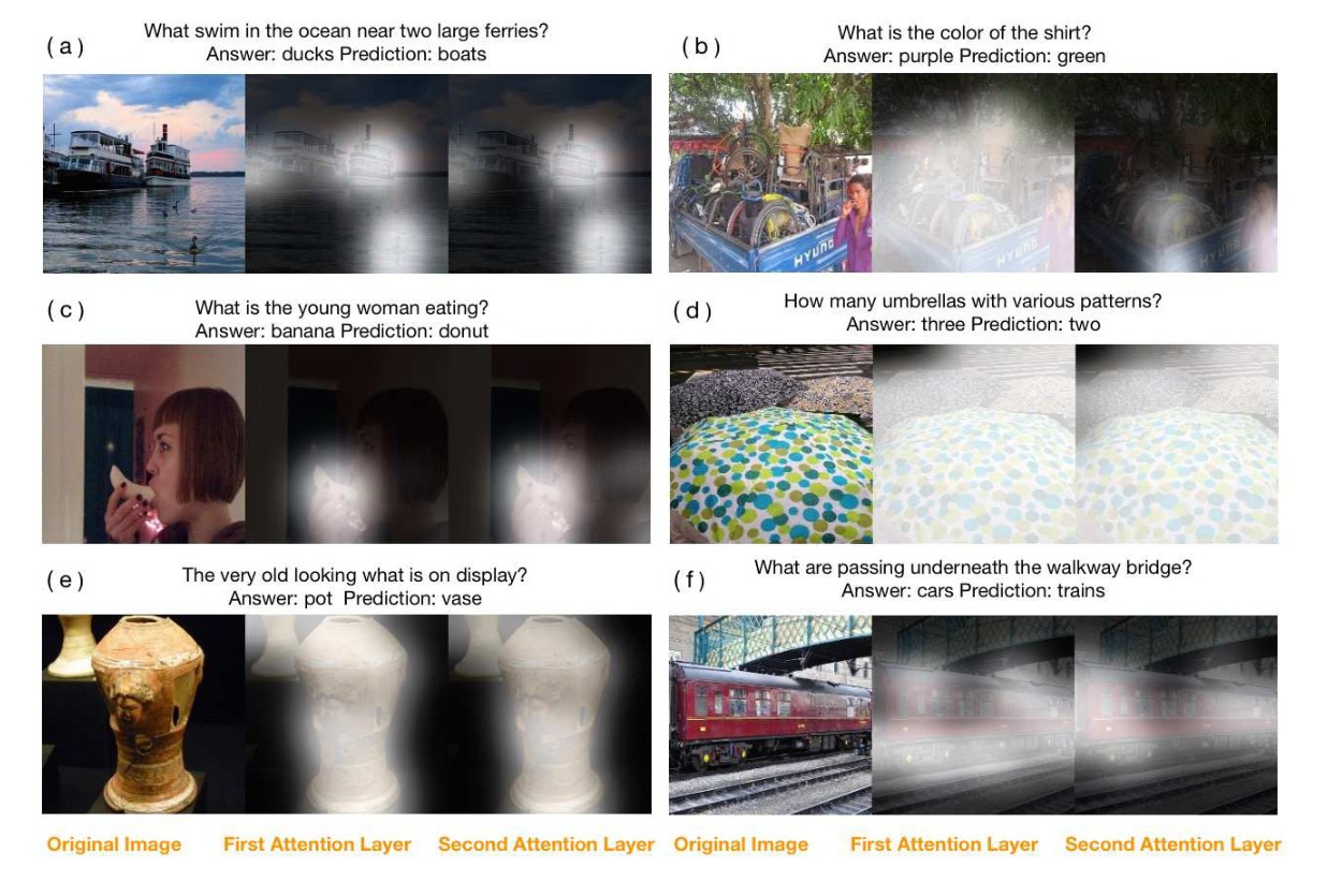
Figure 6: Examples of mistakes
图 6:出错的例子
We randomly sample 100 images from the COCO-QA test set that the SAN make mistakes. We group the errors into four categories: (i) the SANs focus the attention on the wrong regions (22%), e.g., the example in Fig. 6(a); (ii) the SANs focus on the right region but predict a wrong answer (42%), e.g., the examples in Fig. 6(b)(c)(d); (iii) the answer is ambiguous, or the SANs give answers that are different from labels, but might be acceptable (31%). E.g., in Fig. 6(e), the answer label is pot, but our model predicts vase, which is also visually reasonable; (iv) the labels are clearly wrong (5%). E.g., in Fig. 6(f), our model gives the correct answer trains while the label cars is wrong.
我们从 COCO-QA 测试集中随机抽取了 100 张 SAN 出错的图像。我们把错误分成四类:(i) SAN 把注意力放在了错误的区域(22%),例如图 6(a) 中的例子;(ii) SAN 关注了正确区域,但预测了错误答案(42%),例如图 6(b)(c)(d) 中的例子;(iii) 答案本身含糊,或者 SAN 给出的答案与标签不同,但或许可以接受(31%)。例如在图 6(e) 中,答案标签是 pot,但我们的模型预测为 vase,从视觉上看也说得通;(iv) 标签明显标错(5%)。例如在图 6(f) 中,我们的模型给出了正确答案 trains,而标签 cars 是错的。
5. Conclusion
In this paper, we propose a new stacked attention network (SAN) for image QA. SAN uses a multiple-layer attention mechanism that queries an image multiple times to locate the relevant visual region and to infer the answer progressively. Experimental results demonstrate that the proposed SAN significantly outperforms previous state-of-the-art approaches by a great margin on all four image QA data.
本文为图像问答提出一种新的堆叠注意力网络(SAN)。SAN 使用多层注意力机制,对图像多次查询,以定位相关的视觉区域,并逐步推断答案。实验结果表明,所提出的 SAN 在全部四个图像问答数据上都以较大幅度明显超过此前最好方法。
References
[1] S. Antol, A. Agrawal, J. Lu, M. Mitchell, D. Batra, C. L. Zitnick, and D. Parikh. Vqa: Visual question answering. arXiv preprint arXiv:1505.00468, 2015. 1, 2, 5, 6, 7
[2] D. Bahdanau, K. Cho, and Y. Bengio. Neural machine translation by jointly learning to align and translate. arXiv preprint arXiv:1409.0473, 2014. 1
[3] J. Berant and P. Liang. Semantic parsing via paraphrasing. In Proceedings of ACL, volume 7, page 92, 2014. 1
[4] A. Bordes, S. Chopra, and J. Weston. Question answering with subgraph embeddings. arXiv preprint arXiv:1406.3676, 2014. 1
[5] X. Chen and C. L. Zitnick. Learning a recurrent visual representation for image caption generation. arXiv preprint arXiv:1411.5654, 2014. 2
[6] H. Fang, S. Gupta, F. Iandola, R. Srivastava, L. Deng, P. Dollár, J. Gao, X. He, M. Mitchell, J. Platt, et al. From captions to visual concepts and back. arXiv preprint arXiv:1411.4952, 2014. 2, 3, 5
[7] H. Gao, J. Mao, J. Zhou, Z. Huang, L. Wang, and W. Xu. Are you talking to a machine? dataset and methods for multilingual image question answering. arXiv preprint arXiv:1505.05612, 2015. 1, 2
[8] A. Graves. Generating sequences with recurrent neural networks. arXiv preprint arXiv:1308.0850, 2013. 5
[9] S. Hochreiter and J. Schmidhuber. Long short-term memory. Neural computation, 9(8):1735–1780, 1997. 1
[10] A. Karpathy and L. Fei-Fei. Deep visual-semantic alignments for generating image descriptions. arXiv preprint arXiv:1412.2306, 2014. 2
[11] Y. Kim. Convolutional neural networks for sentence classification. arXiv preprint arXiv:1408.5882, 2014. 3
[12] R. Kiros, R. Salakhutdinov, and R. S. Zemel. Unifying visual-semantic embeddings with multimodal neural language models. arXiv preprint arXiv:1411.2539, 2014. 2
[13] A. Krizhevsky, I. Sutskever, and G. E. Hinton. Imagenet classification with deep convolutional neural networks. In Advances in neural information processing systems, pages 1097–1105, 2012. 2
[14] A. Kumar, O. Irsoy, J. Su, J. Bradbury, R. English, B. Pierce, P. Ondruska, I. Gulrajani, and R. Socher. Ask me anything: Dynamic memory networks for natural language processing. arXiv preprint arXiv:1506.07285, 2015. 1
[15] Y. LeCun, L. Bottou, Y. Bengio, and P. Haffner. Gradient-based learning applied to document recognition. Proceedings of the IEEE, 86(11):2278–2324, 1998. 1
[16] T.-Y. Lin, M. Maire, S. Belongie, J. Hays, P. Perona, D. Ramanan, P. Dollár, and C. L. Zitnick. Microsoft coco: Common objects in context. In Computer Vision–ECCV 2014, pages 740–755. Springer, 2014. 5
[17] L. Ma, Z. Lu, and H. Li. Learning to answer questions from image using convolutional neural network. arXiv preprint arXiv:1506.00333, 2015. 2, 5, 6
[18] M. Malinowski and M. Fritz. A multi-world approach to question answering about real-world scenes based on uncertain input. In Advances in Neural Information Processing Systems, pages 1682–1690, 2014. 1, 2, 4, 5, 6
[19] M. Malinowski, M. Rohrbach, and M. Fritz. Ask your neurons: A neural-based approach to answering questions about images. arXiv preprint arXiv:1505.01121, 2015. 1, 2, 5, 6
[20] J. Mao, W. Xu, Y. Yang, J. Wang, and A. Yuille. Deep captioning with multimodal recurrent neural networks (m-rnn). arXiv preprint arXiv:1412.6632, 2014. 2
[21] M. Ren, R. Kiros, and R. Zemel. Exploring models and data for image question answering. arXiv preprint arXiv:1505.02074, 2015. 1, 2, 5, 6
[22] Y. Shen, X. He, J. Gao, L. Deng, and G. Mesnil. A latent semantic model with convolutional-pooling structure for information retrieval. In Proceedings of the 23rd ACM International Conference on Conference on Information and Knowledge Management, pages 101–110. ACM, 2014. 3
[23] K. Simonyan and A. Zisserman. Very deep convolutional networks for large-scale image recognition. arXiv preprint arXiv:1409.1556, 2014. 2
[24] N. Srivastava, G. Hinton, A. Krizhevsky, I. Sutskever, and R. Salakhutdinov. Dropout: A simple way to prevent neural networks from overfitting. The Journal of Machine Learning Research, 15(1):1929–1958, 2014. 5
[25] I. Sutskever, O. Vinyals, and Q. V. Le. Sequence to sequence learning with neural networks. In Advances in neural information processing systems, pages 3104–3112, 2014. 3
[26] C. Szegedy, W. Liu, Y. Jia, P. Sermanet, S. Reed, D. Anguelov, D. Erhan, V. Vanhoucke, and A. Rabinovich. Going deeper with convolutions. arXiv preprint arXiv:1409.4842, 2014. 2
[27] O. Vinyals, A. Toshev, S. Bengio, and D. Erhan. Show and tell: A neural image caption generator. arXiv preprint arXiv:1411.4555, 2014. 2
[28] J. Weston, S. Chopra, and A. Bordes. Memory networks. arXiv preprint arXiv:1410.3916, 2014. 1
[29] Z. Wu and M. Palmer. Verbs semantics and lexical selection. In Proceedings of the 32nd annual meeting on Association for Computational Linguistics, pages 133–138. Association for Computational Linguistics, 1994. 5
[30] K. Xu, J. Ba, R. Kiros, A. Courville, R. Salakhutdinov, R. Zemel, and Y. Bengio. Show, attend and tell: Neural image caption generation with visual attention. arXiv preprint arXiv:1502.03044, 2015. 1, 2
[31] W.-t. Yih, M.-W. Chang, X. He, and J. Gao. Semantic parsing via staged query graph generation: Question answering with knowledge base. In Proceedings of the Joint Conference of the 53rd Annual Meeting of the ACL and the 7th International Joint Conference on Natural Language Processing of the AFNLP, 2015. 1
[32] W.-t. Yih, X. He, and C. Meek. Semantic parsing for single-relation question answering. In Proceedings of ACL, 2014. 1