On the Spectral Bias of Neural Networks
On the Spectral Bias of Neural Networks
*Equal contribution
Mila, Quebec, Canada Image Analysis and Learning Lab, Ruprecht-Karls-Universität Heidelberg, Germany. Correspondence to: Nasim Rahaman nasim.rahaman@live.com, Aristide Baratin aristide.baratin@umontreal.ca, Devansh Arpit devansharpit@gmail.com.
Proceedings of the 36th International Conference on Machine Learning, Long Beach, California, PMLR 97, 2019. Copyright 2019 by the author(s).
Abstract
摘要
Neural networks are known to be a class of highly expressive functions able to fit even random input-output mappings with accuracy. In this work we present properties of neural networks that complement this aspect of expressivity. By using tools from Fourier analysis, we highlight a learning bias of deep networks towards low frequency functions – i.e. functions that vary globally without local fluctuations – which manifests itself as a frequency-dependent learning speed. Intuitively, this property is in line with the observation that over-parameterized networks prioritize learning simple patterns that generalize across data samples. We also investigate the role of the shape of the data manifold by presenting empirical and theoretical evidence that, somewhat counter-intuitively, learning higher frequencies gets easier with increasing manifold complexity.
神经网络被视为一类表达能力很强的函数,甚至能以 的准确率拟合随机的输入–输出映射。在本文中,我们给出一些与这种表达能力形成补充的性质。借助傅里叶分析,我们指出深度网络在学习上偏向低频函数,也就是在全局上变化、而没有局部起伏的函数;这一偏向表现为与频率有关的学习速度。直观上,这与下述观察一致:过参数化网络会优先学习能在数据样本之间泛化的简单模式。我们还研究了数据流形形状的作用,并给出经验和理论证据:有些反直觉的是,流形越复杂,学习更高频率反而会变得更容易。
1. Introduction
1. 引言
The remarkable success of deep neural networks at generalizing to natural data is at odds with the traditional notions of model complexity and their empirically demonstrated ability to fit arbitrary random data to perfect accuracy (Zhang et al., 2017a; Arpit et al., 2017). This has prompted recent investigations of possible implicit regularization mechanisms inherent in the learning process which induce a bias towards low complexity solutions (Neyshabur et al., 2014; Soudry et al., 2017; Poggio et al., 2018; Neyshabur et al., 2017).
深度神经网络在自然数据上的泛化表现相当突出,这与传统的模型复杂度观念,以及它们被经验证明能够把任意随机数据拟合到完美准确率这一事实,并不一致(Zhang et al., 2017a; Arpit et al., 2017)。这促使人们近来去考察学习过程中可能固有的隐式正则机制,这类机制会诱导模型偏向低复杂度解(Neyshabur et al., 2014; Soudry et al., 2017; Poggio et al., 2018; Neyshabur et al., 2017)。
In this work, we take a slightly shifted view on implicit regularization by suggesting that low-complexity functions are learned faster during training by gradient descent. We expose this bias by taking a closer look at neural networks through the lens of Fourier analysis. While they can approximate arbitrary functions, we find that these networks prioritize learning the low frequency modes, a phenomenon we call the spectral bias. This bias manifests itself not just in the process of learning, but also in the parameterization of the model itself: in fact, we show that the lower frequency components of trained networks are more robust to random parameter perturbations. Finally, we also expose and analyze the rather intricate interplay between the spectral bias and the geometry of the data manifold by showing that high frequencies get easier to learn when the data lies on a lower-dimensional manifold of complex shape embedded in the input space of the model. We focus the discussion on networks with rectified linear unit (ReLU) activations, whose continuous piece-wise linear structure enables an analytic treatment.
在本文中,我们对隐式正则采取一个略有移动的视角:认为低复杂度函数在用梯度下降训练时会被更快地学会。我们从傅里叶分析的角度更仔细地考察神经网络,从而揭示这一偏向。尽管它们可以逼近任意函数,我们却发现这些网络会优先学习低频模态,我们把这一现象称为频谱偏置(spectral bias)。这一偏置不仅出现在学习过程中,也体现在模型的参数化本身:事实上,我们表明,训练好的网络中,低频分量对随机参数扰动更为稳健。最后,我们还揭示并分析了频谱偏置与数据流形几何之间相当细致的相互作用:当数据落在嵌入模型输入空间、形状复杂的低维流形上时,高频会变得更容易学习。讨论集中在采用整流线性单元(ReLU)激活的网络上,其连续分段线性结构使得解析处理成为可能。
Contributions
贡献
- We exploit the continuous piecewise-linear structure of ReLU networks to evaluate its Fourier spectrum (Section 2).
- 我们利用 ReLU 网络的连续分段线性结构,来计算其傅里叶谱(第 2 节)。
- We find empirical evidence of a spectral bias: i.e. lower frequencies are learned first. We also show that lower frequencies are more robust to random perturbations of the network parameters (Section 3).
- 我们找到了频谱偏置的经验证据:也就是低频会先被学会。我们还表明,低频对网络参数的随机扰动更为稳健(第 3 节)。
- We study the role of the shape of the data manifold: we show how complex manifold shapes can facilitate the learning of higher frequencies and develop a theoretical understanding of this behavior (Section 4).
- 我们研究数据流形形状的作用:说明复杂的流形形状如何有助于学习更高频率,并对此行为给出理论理解(第 4 节)。
2. Fourier analysis of ReLU networks
2. ReLU 网络的傅里叶分析
2.1. Preliminaries
2.1. 预备知识
Throughout the paper we call ‘ReLU network’ a scalar function defined by a neural network with hidden layers of widths and a single output neuron:
在全文中,我们把“ReLU 网络”称作由一个具有 个隐层(宽度为 )以及单个输出神经元的神经网络所定义的标量函数 :
where each is an affine function ( and ) and denotes the ReLU activation function acting elementwise on a vector . In the standard basis, for some weight matrix and bias vector .
其中每个 是仿射函数( 且 ), 表示作用在向量 各个分量上的 ReLU 激活函数。在标准基下,,其中 是权重矩阵, 是偏置向量。
ReLU networks are known to be continuous piece-wise linear (CPWL) functions, where the linear regions are convex polytopes (Raghu et al., 2016; Montufar et al., 2014; Zhang et al., 2018; Arora et al., 2018). Remarkably, the converse also holds: every CPWL function can be represented by a ReLU network (Arora et al., 2018, Theorem 2.1), which in turn endows ReLU networks with universal approximation properties. Given the ReLU network from Eqn. 1, we can make the piecewise linearity explicit by writing,
已知 ReLU 网络是连续分段线性(CPWL)函数,其线性区域是凸多面体(Raghu et al., 2016; Montufar et al., 2014; Zhang et al., 2018; Arora et al., 2018)。值得注意的是,反过来也成立:每个 CPWL 函数都可以由 ReLU 网络表示(Arora et al., 2018, Theorem 2.1),这进而赋予 ReLU 网络普遍逼近性质。给定式 1 中的 ReLU 网络 ,我们可以把分段线性显式地写成,
where is an index for the linear regions and is the indicator function on . As shown in Appendix B in more detail, each region corresponds to an activation pattern of all hidden neurons of the network, which is a binary vector with components conditioned on the sign of the input of the respective neuron. The matrix is given by
其中 是线性区域 的索引, 是 上的示性函数。如附录 B 中更详细表明的,每个区域对应于网络全部隐神经元的一个激活模式,这是一个二进制向量,其分量取决于相应神经元输入的符号。 矩阵 由下式给出
We adopt the terminology of Raghu et al. (2016); Montufar et al. (2014).
我们采用 Raghu et al. (2016); Montufar et al. (2014) 的术语。
where is obtained from the original weight by setting its column to zero whenever the neuron of the layer is inactive.
其中 是从原始权重 得到的:只要第 层的神经元 处于未激活状态,就把其第 列置零。
2.2. Fourier Spectrum
2.2. 傅里叶谱
In the following, we study the structure of ReLU networks in terms of their Fourier representation, , where is the Fourier transform. Lemmas 1 and 2 yield the explicit form of the Fourier components (we refer to Appendix C for the proofs and technical details).
接下来,我们从傅里叶表示的角度研究 ReLU 网络的结构,,其中 是傅里叶变换。引理 1 和引理 2 给出了傅里叶分量的显式形式(证明与技术细节见附录 C)。
Note that general ReLU networks need not be squared integrable: for instance, the class of two-layer ReLU networks represent an arrangement of hyperplanes (Montufar et al., 2014) and hence grow linearly as . In such cases, the Fourier transform is to be understood in the sense of tempered distributions acting on rapidly decaying smooth functions as . See Appendix C for a formal treatment.
注意,一般的 ReLU 网络不一定平方可积:例如,两层 ReLU 网络表示的是一组超平面排布(Montufar et al., 2014),因此会随 线性增长。在这类情形中,傅里叶变换应在缓增分布的意义下理解,它作用在快速衰减的光滑函数 上,满足 。形式处理见附录 C。
Lemma 1.
引理 1。
The Fourier transform of ReLU networks decomposes as,
ReLU 网络的傅里叶变换可分解为
where and is the Fourier transform of the indicator function of .
其中 ,且 是 的示性函数的傅里叶变换。
The Fourier transform of the indicator over linear regions appearing in Eqn. 4 are fairly intricate mathematical objects. Diaz et al. (2016) develop an elegant procedure for evaluating it in arbitrary dimensions via a recursive application of Stokes theorem. We describe this procedure in detail in Appendix C.2, and present here its main corollary.
式 4 中出现的、线性区域示性函数的傅里叶变换,是相当精细的数学对象。Diaz et al. (2016) 发展了一种优雅的方法,通过递归应用 Stokes 定理,在任意维中计算它。我们在附录 C.2 中详细描述这一方法,并在此给出其主要推论。
We also generalize the construction to tempered distributions.
我们也将该构造推广到缓增分布。
Lemma 2.
引理 2。
Let be a full dimensional polytope in . Its Fourier spectrum takes the form:
设 是 中的一个满维多面体。其傅里叶谱具有如下形式:
where is the union of -dimensional subspaces that are orthogonal to some -codimensional face of , is in and the indicator over .
其中 是与 的某个余维为 的面正交的 维子空间的并, 属于 ,而 是 上的示性函数。
Lemmas 1, 2 together yield the main result of this section.
引理 1 与引理 2 合在一起,得到本节的主要结果。
Theorem 1.
定理 1。
The Fourier components of the ReLU network with parameters is given by the rational function:
参数为 的 ReLU 网络 的傅里叶分量由如下有理函数给出:
where is the union of -dimensional subspaces that are orthogonal to some -codimensional faces of some polytope and is .
其中 是与某个多面体 的某些余维为 的面正交的 维子空间的并,且 是 。
Note that Eqn 6 applies to general ReLU networks with arbitrary width and depth.
注意,式 6 适用于任意宽度和深度的一般 ReLU 网络。
Symmetries that might arise due to additional assumptions can be used to further develop Eqn 6, see e.g. Eldan & Shamir (2016) for 2-layer networks.
若有额外假设带来的对称性,还可用来进一步展开式 6,例如可参见 Eldan & Shamir (2016) 对两层网络的讨论。
Discussion. We make the following two observations. First, the spectral decay of ReLU networks is highly anisotropic in large dimensions. In almost all directions of , we have a decay. However, the decay can be as slow as in specific directions orthogonal to the dimensional faces bounding the linear regions.
讨论。 我们有以下两点观察。第一,在高维中,ReLU 网络的谱衰减是高度各向异性的。在 的几乎所有方向上,衰减是 。但在与界定线性区域的 维面正交的特定方向上,衰减可以慢到 。
Note that such a rate is not guaranteed by piecewise smoothness alone. For instance, the function is continuous and smooth everywhere except at , yet it decays as in the Fourier domain.
注意,这样的速率并不能仅由分段光滑保证。例如,函数 除了在 处以外处处连续且光滑,但它在傅里叶域中按 衰减。
Second, the numerator in Eqn 6 is bounded by (cf. Appendix C.3), where is the number of linear regions and is the Lipschitz constant of the network. Further, the Lipschitz constant can be bounded as (cf. Appendix C.6):
第二,式 6 中的分子以 为界(参见附录 C.3),其中 是线性区域的个数, 是网络的 Lipschitz 常数。此外, 可以按如下方式界定(参见附录 C.6):
where is the spectral norm and the max norm, and is the number of units in the -th layer. This makes the bound on scale exponentially in depth and polynomial in width. As for the number of linear regions, Montufar et al. (2014) and Raghu et al. (2016) obtain tight bounds that exhibit the same scaling behaviour (Raghu et al., 2016, Theorem 1). In Appendix A.5, we qualitatively ablate over the depth and width of the network to expose how this reflects on the Fourier spectrum of the network.
其中 是谱范数, 是最大范数, 是第 层的单元数。这使 的上界随深度指数增长、随宽度多项式增长。至于线性区域个数 ,Montufar et al. (2014) 和 Raghu et al. (2016) 得到了具有同样标度行为的紧界(Raghu et al., 2016, Theorem 1)。在附录 A.5 中,我们定性地消融网络的深度和宽度,以展示这如何反映在网络的傅里叶谱上。
3. Lower Frequencies are Learned First
3. 低频会先被学会
We now present experiments showing that networks tend to fit lower frequencies first during training. We refer to this phenomenon as the spectral bias, and discuss it in light of the results of Section 2.
接下来给出实验,表明网络在训练中往往先拟合较低频率。我们把这一现象称作频谱偏置,并结合第 2 节的结果加以讨论。
3.1. Synthetic Experiments
3.1. 合成实验
Experiment 1.
实验 1。
The setup is as follows: Given frequencies with corresponding amplitudes , and phases , we consider the mapping given by
实验设置如下:给定频率 、对应振幅 以及相位 ,我们考虑映射 ,其定义为
More experimental details and additional plots are provided in Appendix A.1.
更多实验细节与补充图见附录 A.1。
A 6-layer deep 256-unit wide ReLU network is trained to regress with and input samples spaced equally over ; its spectrum in expectation over is monitored as training progresses. In the first setting, we set equal amplitude for all frequencies and in the second setting, the amplitude increases from to . Figure 1 shows the normalized magnitudes at various frequencies, as training progresses with full-batch gradient descent. Further, Figure 2 shows the learned function at intermediate training iterations. The result is that lower frequencies (i.e. smaller 's) are regressed first, regardless of their amplitudes.
我们用一个 6 层、每层 256 个单元的 ReLU 网络 去回归 ,频率取 ,在 上均匀取 个输入样本;训练过程中监控其频谱 对 的期望。第一种设置里,各频率振幅相等,;第二种设置里,振幅从 递增到 。图 1 给出全批量梯度下降训练过程中,各频率上的归一化幅值 。图 2 则给出若干中间迭代步上学到的函数。结果表明,无论振幅如何,较低频率(即较小的 )都会先被回归出来。
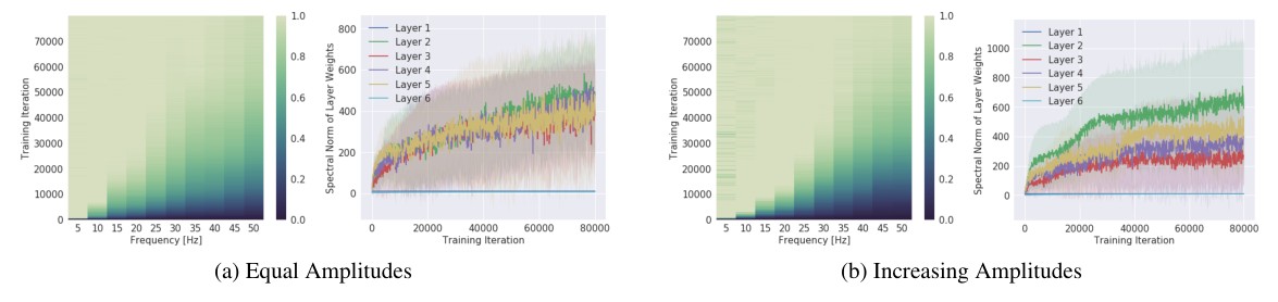
Figure 1. Left (a, b): Evolution of the spectrum (x-axis for frequency) during training (y-axis). The colors show the measured amplitude of the network spectrum at the corresponding frequency, normalized by the target amplitude at the same frequency (i.e. ) and the colorbar is clipped between 0 and 1. Right (a, b): Evolution of the spectral norm (y-axis) of each layer during training (x-axis). Figure-set (a) shows the setting where all frequency components in the target function have the same amplitude, and (b) where higher frequencies have larger amplitudes. Gist: We find that even when higher frequencies have larger amplitudes, the model prioritizes learning lower frequencies first. We also find that the spectral norm of weights increases as the model fits higher frequency, which is what we expect from Theorem 1.
图 1. 左(a、b):训练过程中(纵轴)频谱(横轴为频率)的演变。颜色表示网络频谱在对应频率上测得的振幅,并按同一频率上的目标振幅做了归一化(即 ),色条裁剪在 0 到 1 之间。右(a、b):训练过程中(横轴)各层谱范数(纵轴)的演变。图组 (a) 是目标函数各频率分量振幅相同的设置,(b) 是更高频率具有更大振幅的设置。要点:即便更高频率的振幅更大,模型仍会优先学习较低频率。我们还发现,随着模型拟合更高频率,权重的谱范数会增大,这与定理 1 的预期一致。
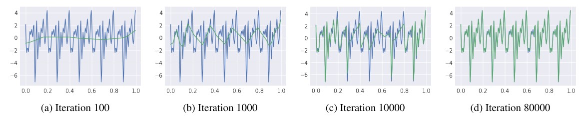
Figure 2. The learnt function (green) overlayed on the target function (blue) as the training progresses. The target function is a superposition of sinusoids of frequencies , equal amplitudes and randomly sampled phases.
图 2. 训练过程中学到的函数(绿色)叠加在目标函数(蓝色)上。目标函数是频率为 的正弦波叠加,各分量振幅相等,相位随机取样。
Experiment 2.
实验 2。
Our goal here is to illustrate a phenomenon that complements the one highlighted above: lower frequencies are more robust to parameter perturbations. The set up is the same as in Experiment 1. The network is trained to regress a target function with frequencies and amplitudes . After convergence to , we consider random (isotropic) perturbations of given magnitude , where is a random unit vector in parameter space. We evaluate the network function at the perturbed parameters, and compute the magnitude of its discrete Fourier transform at frequencies to obtain . We also average over 100 samples of to obtain , which we normalize by . Finally, we average over the phases (see Eqn 8). The result, shown in Figure 3, demonstrates that higher frequencies are significantly less robust than the lower ones, guiding the intuition that expressing higher frequencies requires the parameters to be finely-tuned to work together. In other words, parameters that contribute towards expressing high-frequency components occupy a small volume in the parameter space. We formalize this in Appendix D.
这里要说明的,是与上一现象互补的另一点:较低频率对参数扰动更加稳健。设置与实验 1 相同。网络被训练去回归一个目标函数,频率为 ,振幅 。收敛到 之后,我们考虑给定幅度 的随机(各向同性)扰动 ,其中 是参数空间中的随机单位向量。我们在扰动后的参数上计算网络函数 ,并取其离散傅里叶变换在频率 处的幅值,得到 。再对 100 个 样本取平均,得到 ,并用 做归一化。最后对相位 取平均(见式 8)。图 3 的结果显示,高频明显不如低频稳健,这提示我们:要表达更高频率,参数必须彼此精细配合。换句话说,对表达高频分量有贡献的那些参数,在参数空间里只占很小的体积。我们在附录 D 中把它形式化。
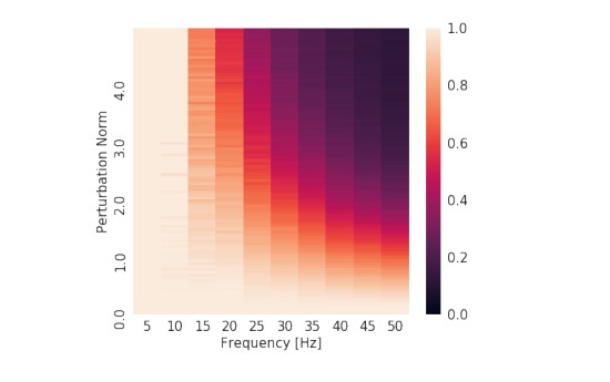
Figure 3. Normalized spectrum of the model (x-axis for frequency, colorbar for magnitude) with perturbed parameters as a function of parameter perturbation (y-axis). The colormap is clipped between 0 and 1. We observe that the lower frequencies are more robust to parameter perturbations than the higher frequencies.
图 3. 参数受到扰动后,模型的归一化频谱(横轴为频率,色条表示幅值)随参数扰动(纵轴)的变化。颜色映射裁剪在 0 到 1 之间。可以看到,较低频率比更高频率对参数扰动更为稳健。
Discussion. Multiple theoretical aspects may underlie these observations. First, for a fixed architecture, recall that the numerator in Theorem 1 is (where is the Lipschitz constant of the function). However, is bounded by the parameter norm, which can only increase gradually during training by gradient descent. This leads to the higher frequencies being learned late in the optimization process. To confirm that the bound indeed increases as the model fits higher frequencies, we plot in Fig 1 the spectral norm of weights of each layer during training for both cases of constant and increasing amplitudes.
讨论。 这些观察背后可能有多层理论原因。首先,对固定结构而言,定理 1 中的分子是 (其中 是该函数的 Lipschitz 常数)。但 受参数范数约束,而在梯度下降训练中,参数范数只能逐渐增大。于是更高频率往往要到优化过程的较晚阶段才会被学会。为确认该上界确实会随着模型拟合更高频率而增大,我们在图 1 中画出了恒定振幅与递增振幅两种情形下,各层权重谱范数随训练的变化。
The tightness of this bound is verified empirically in appendix A.5.
该上界的松紧程度在附录 A.5 中用经验结果做了验证。
This assumes that the Lipschitz constant of the (noisy) target function is larger than that of the network at initialization.
这里假定(含噪声的)目标函数的 Lipschitz 常数大于网络在初始化时的 Lipschitz 常数。
Second (cf. Appendix C.4), the exact form of the Fourier spectrum yields that for a fixed direction , the spectral decay rate of the parameter gradient is at most one exponent of lower than that of . If for a fixed we have where , we obtain for the residual and (continuous) training step :
其次(参见附录 C.4),由傅里叶变换的精确形式可知:对固定方向 ,参数梯度 的频谱衰减率,最多只比 低 的一个指数。若对固定的 有 ,其中 ,则对残差 以及(连续)训练步 ,可得:
where we use the fact that is just the learning rate times the parameter gradient of the loss which is independent of , and assume that the target function is fixed. Eqn 9 shows that the rate of change of the residual decays with increasing frequency, which is what we find in Experiment 1.
这里用到: 就是学习率乘以损失对参数的梯度,它与 无关;并假定目标函数 固定。式 9 表明,残差的变化率会随频率升高而衰减,这与实验 1 的发现一致。
Note however that the loss term might involve a sum or an integral over all frequencies, but the summation is over a different variable.
不过需要指出,损失项可能包含对所有频率的求和或积分,但那个求和是对另一个变量进行的。
3.2. Real-Data Experiments
3.2. 真实数据实验
While Experiments 1 and 2 establish the spectral bias by explicitly evaluating the Fourier coefficients, doing so becomes prohibitively expensive for larger (e.g. on MNIST). To tackle this, we propose the following set of experiments to measure the effect of spectral bias indirectly on MNIST.
实验 1 和 2 是通过直接计算傅里叶系数来确立频谱偏置的;但当 较大时(例如在 MNIST 上),这样做会过于昂贵。为此,我们提出下面一组实验,在 MNIST 上间接度量频谱偏置的影响。
Experiment 3.
实验 3。
In this experiment, we investigate how the validation performance dependent on the frequency of noise added to the training target. We find that the best validation performance on MNIST is particularly insensitive to the magnitude of high-frequency noise, yet it is adversely affected by low-frequency noise. We consider a target (binary) function defined on the space of MNIST inputs. Samples form a subset of the MNIST dataset comprising samples belonging to two classes. Let be a noise function:
本实验考察验证表现如何依赖于加在训练目标上的噪声频率。我们发现,MNIST 上最好的验证表现对高频噪声的幅度特别不敏感,却会受到低频噪声的不利影响。我们考虑定义在 MNIST 输入空间 上的目标(二值)函数 。样本 取自 MNIST 中属于两个类别的子集。设 为噪声函数:
corresponding to a radial wave defined on the -dimensional input space. The final target function is then given by , where is the effective amplitude of the noise. We fit the same network as in Experiment 1 to the target with the MSE loss. In the first set of experiments, we ablate over for a pair of fixed s, while in the second set we ablate over for a pair of fixed s. In Figure 4, we show the respective validation loss curves, where the validation set is obtained by evaluating on a separate subset of the data, i.e. . Figure 11 (in appendix A.3) shows the respective training curves.
它对应定义在 维输入空间上的径向波。最终目标函数为 ,其中 是噪声的有效振幅。我们用与实验 1 相同的网络,以 MSE 损失拟合目标 。第一组实验在一对固定的 下对 做消融,第二组实验在一对固定的 下对 做消融。图 4 给出相应的验证损失曲线;验证集是在另一数据子集上对 求值得到的,即 。相应的训练曲线见附录 A.3 的图 11。
The rationale behind using a radial wave is that it induces oscillations (simultaneously) along all spatial directions. Another viable option is to induce oscillations along the principle axes of the data: we have verified that the key trends of interest are preserved.
采用径向波的理由是,它会(同时)沿所有空间方向诱发振荡。另一种可行做法是沿数据的主轴诱发振荡:我们已验证,所关心的主要趋势仍然保持。
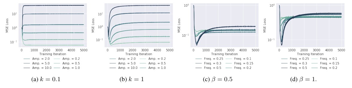
Figure 4. (a,b,c,d): Validation curves for various settings of noise amplitude and frequency . The corresponding training curves can be found in Figure 11 in appendix A.3. Gist: Low frequency noise affects the network more than their high-frequency counterparts. Further, for high-frequency noise, one finds that the validation loss dips early in the training. Both these observations are explained by the fact that network readily fit lower frequencies, but learn higher frequencies later in the training.
图 4. (a,b,c,d):在不同噪声振幅 与频率 设置下的验证曲线。相应的训练曲线见附录 A.3 的图 11。要点:低频噪声对网络的影响大于其高频对应物。此外,对于高频噪声,验证损失会在训练早期出现低谷。这两种观察都可以用下述事实解释:网络很容易拟合较低频率,而更高频率要到训练较晚阶段才会被学会。
Discussion. The profile of the loss curves varies significantly with the frequency of noise added to the target. In Figure 4(a), we see that the validation performance is adversely affected by the amplitude of the low-frequency noise, whereas Figure 4(b) shows that the amplitude of high-frequency noise does not significantly affect the best validation score. This is explained by the fact that the network readily fits the noise signal if it is low frequency, whereas the higher frequency noise is only fit later in the training. In the latter case, the dip in validation score early in the training is when the network has learned the low frequency true target function ; the remainder of the training is spent learning the higher-frequencies in the training target , as we shall see in the next experiment. Figures 4(c) and 4(d) confirm that the dip in validation score exacerbates for increasing frequency of the noise. Further, we observe that for higher frequencies (e.g. ), increasing the amplitude does not significantly degrade the best performance at the dip, confirming that the network is fairly robust to the amplitude of high-frequency noise.
讨论。 损失曲线的形态会随加在目标上的噪声频率而明显变化。图 4(a) 显示,验证表现会受到低频噪声幅度的不利影响;而图 4(b) 显示,高频噪声的幅度并不会显著改变最好的验证分数。原因在于:噪声若是低频,网络很容易把它拟合进去;高频噪声则要到训练较晚阶段才会被拟合。后一种情形里,训练早期验证分数出现低谷,正是网络已经学会低频真实目标函数 的时候;余下的训练则用来学习训练目标 中的更高频率,下一实验将说明这一点。图 4(c) 和 4(d) 进一步确认,噪声频率越高,验证分数的低谷越深。我们还观察到,在更高频率(例如 )上,增大振幅 并不会显著恶化低谷处的最好表现,说明网络对高频噪声的幅度相当稳健。
Finally, we note that the dip in validation score was also observed by Arpit et al. (2017) with i.i.d. noise in a classification setting.
最后我们指出,Arpit et al. (2017) 在分类设定中使用独立同分布噪声时,也观察到了验证分数的这一低谷。
Recall that i.i.d. noise is white-noise, which has a constant Fourier spectrum magnitude in expectation, i.e. it also contains high-frequency components.
回想一下,独立同分布噪声就是白噪声,其傅里叶频谱幅值在期望上为常数,也就是说其中也包含高频分量。
Experiment 4.
实验 4。
To investigate the dip observed in Experiment 3, we now take a more direct approach by considering a generalized notion of frequency. To that end, we project the network function to the space spanned by the orthonormal eigenfunctions of the Gaussian RBF kernel (Braun et al., 2006). These eigenfunctions (sorted by decreasing eigenvalues) resemble sinusoids (Fasshauer, 2011), and the index can be thought of as being a proxy for the frequency, as can be seen from Figure 6 (see Appendix A.4 for additional details and supporting plots). While we will call as the spectrum of the function , it should be understood as , where and on the MNIST samples . This allows us to define a noise function as:
为考察实验 3 中看到的低谷,我们改用更直接的办法,引入一种广义的频率概念。为此,把网络函数投影到高斯 RBF 核的标准正交特征函数 所张成的空间上(Braun et al., 2006)。这些特征函数 (按特征值递减排序)形状接近正弦波(Fasshauer, 2011),下标 可以看作频率的代理,这一点可从图 6 看出(更多细节与辅助图见附录 A.4)。我们虽把 称作函数 的频谱,其含义应理解为 ,其中 ,并在 MNIST 样本 上满足 。于是可以把噪声函数定义为:
where is the number of available samples and . Like in Experiment 3, the target function is given by , and the same network is trained to regress . Figure 5 shows the (generalized) spectrum and , and that of as training progresses. Figure 13 (in appendix) shows the corresponding dip in validation loss, where the validation set is same as the training set but with true target function instead of the noised target .
其中 是可用样本数,。与实验 3 一样,目标函数为 ,并用同一网络去回归 。图 5 给出 与 的(广义)频谱,以及训练过程中 的频谱。附录中的图 13 给出相应的验证损失低谷;验证集与训练集相同,只是目标改用真实函数 ,而不是加噪目标 。
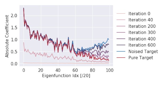
Figure 5. Spectrum of the network as it is trained on MNIST target with high-frequency noise (Noised Target). We see that the network fits the true target at around the th iteration, which is when the validation score dips (Figure 13 in appendix).
图 5. 网络在带有高频噪声的 MNIST 目标(加噪目标)上训练时的频谱。可以看到,网络大约在第 次迭代时拟合了真实目标,而验证分数的低谷也出现在这一时刻(见附录图 13)。
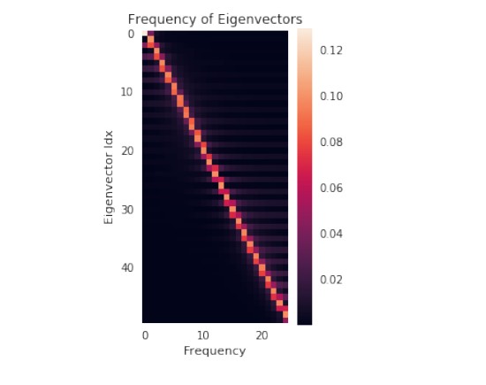
Figure 6. Spectrum (x-axis for frequency, colorbar for magnitude) of the -th (y-axis) eigenvector of the Gaussian RBF kernel matrix , where the sample set is is uniformly spaced points between and and is the Gaussian RBF kernel function. Gist: The eigenfunctions with increasing roughly correspond to sinusoids of increasing frequency. Refer to Appendix A.4 for more details.
图 6. 高斯 RBF 核矩阵 第 个(纵轴)特征向量的频谱(横轴为频率,色条表示幅值);样本集 是 到 之间均匀分布的 个点, 是高斯 RBF 核函数。要点:随着 增大,特征函数大致对应频率逐渐升高的正弦波。更多细节见附录 A.4。
Discussion. From Figure 5, we learn that the drop in validation score observed in Figure 4 is exactly when the higher-frequencies of the noise signal are yet to be learned. As the network gradually learns the higher frequency eigenfunctions, the validation loss increases while the training loss continues to decrease. Thus these experiments show that the phenomenon of spectral bias persists on non-synthetic data and in high dimensional input spaces.
讨论。 由图 5 可见,图 4 中验证分数下降的时刻,恰好是噪声信号中的更高频率尚未被学会之时。随着网络逐渐学会更高频率的特征函数,验证损失上升,训练损失则继续下降。因此这些实验表明,频谱偏置这一现象在非合成数据以及高维输入空间中依然存在。
4. Not all Manifolds are Learned Equal
4. 并非所有流形都被同等学会
In this section, we investigate subtleties that arise when the data lies on a lower dimensional manifold embedded in the higher dimensional input space of the model. We find that the shape of the data-manifold impacts the learnability of high frequencies in a non-trivial way. As we shall see, this is because low frequency functions in the input space may have high frequency components when restricted to lower dimensional manifolds of complex shapes. We demonstrate results in an illustrative minimal setting, free from unwanted confounding factors, and present a theoretical analysis of the phenomenon.
本节考察当数据落在嵌入模型更高维输入空间的低维流形上时会出现的一些细微之处。我们发现,数据流形的形状会以并非平凡的方式影响高频的可学性。原因在于:输入空间中的低频函数,限制到形状复杂的低维流形上时,可能带有高频分量。我们在一个便于说明、并排除多余混杂因素的最小设置中展示结果,并对这一现象给出理论分析。
We include additional experiments on MNIST and CIFAR-10 in appendices A.6 and A.7.
我们在附录 A.6 和 A.7 中补充了 MNIST 与 CIFAR-10 上的实验。
Manifold hypothesis. We consider the case where the data lies on a lower dimensional data manifold embedded in input space (Goodfellow et al., 2016), which we assume to be the image of some injective mapping defined on a lower dimensional latent space . Under this hypothesis and in the context of the standard regression problem, a target function defined on the data manifold can be identified with a function defined on the latent space. Regressing is therefore equivalent to finding such that matches . Further, assuming that the data probability distribution supported on is induced by from the uniform distribution in the latent space , the mean square error can be expressed as:
流形假设。 我们考虑数据落在嵌入输入空间的低维数据流形 上的情形(Goodfellow et al., 2016),并假定它是某个单射映射 在低维潜空间 上的像 。在这一假设以及标准回归问题下,定义在数据流形上的目标函数 可以等同于定义在潜空间上的函数 。因此,回归 等价于寻找 ,使得 与 一致。进一步,若假定支撑在 上的数据概率分布 是由 从潜空间 上的均匀分布 诱导而来,则均方误差可以写成:
Observe that there is a vast space of degenerate solutions that minimize the mean squared error – namely all functions on that yield the same function when restricted to the data manifold .
可以看到,使均方误差最小的退化解 构成一个很大的空间——也就是所有限制到数据流形 上会给出同一函数的、定义在 上的函数。
Our findings from the previous section suggest that neural networks are biased towards expressing a particular subset of such solutions, namely those that are low frequency. It is also worth noting that there exist methods that restrict the space of solutions: notably adversarial training (Goodfellow et al., 2014) and Mixup (Zhang et al., 2017b).
上一节的发现表明,神经网络偏向于表达这类解中的一个特定子集,也就是那些低频的解。还值得指出的是,已有一些方法会限制解空间,尤其是对抗训练(Goodfellow et al., 2014)和 Mixup(Zhang et al., 2017b)。
Experimental set up. The experimental setting is designed to afford control over both the shape of the data manifold and the target function defined on it. We will consider the family of curves in generated by mappings given by
实验设置。 该实验设定旨在同时控制数据流形的形状以及定义在其上的目标函数。我们将考虑由映射 在 中生成的一类曲线,其定义为
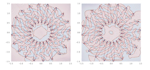
Figure 7. Functions learned by two identical networks (up to initialization) to classify the binarized value of a sine wave of frequency defined on a manifold. Both yield close to perfect accuracy for the samples defined on the manifold (scatter plot), yet they differ significantly elsewhere. The shaded regions show the predicted class (Red or Blue) whereas contours show the confidence (absolute value of logits).
图 7. 两个除初始化外完全相同的网络,在 流形上对频率 的正弦波二值化取值做分类时学到的函数。两者在流形上的样本(散点)上都能达到接近完美的准确率,但在其他位置却相差很大。阴影区域表示预测类别(红或蓝),等高线表示置信度(logits 的绝对值)。
Here, defines the data-manifold and corresponds to a flower-shaped curve with petals, or a unit circle when (see e.g. Fig 7). Given a signal defined on the latent space , the task entails learning a network such that matches the signal .
这里, 定义了数据流形,对应有 个花瓣的花形曲线;当 时则是单位圆(参见图 7)。给定定义在潜空间 上的信号 ,任务是学习一个网络 ,使得 与信号 一致。
Experiment 5.
实验 5。
The set-up is similar to that of Experiment 1, and is as defined in Eqn. 8 with frequencies , and amplitudes . The model is trained on the dataset with uniformly spaced samples between and . The spectrum of in expectation over is monitored as training progresses, and the result is shown in Fig 8 for various . Fig 8(e) shows the corresponding mean squared error curves. More experimental details in appendix A.2.
设置与实验 1 类似, 的定义见式 8,频率取 ,振幅 。模型 在数据集 上训练,其中 ,样本 在 到 之间均匀分布。训练过程中监控 对 的期望频谱,不同 下的结果见图 8。图 8(e) 给出相应的均方误差曲线。更多实验细节见附录 A.2。
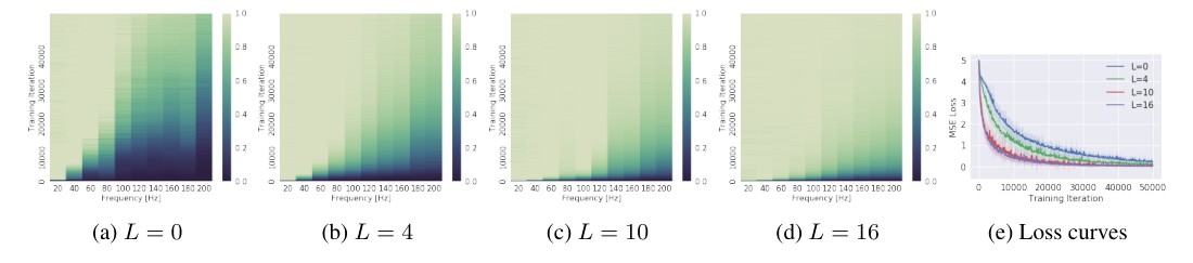
Figure 8. (a,b,c,d): Evolution of the network spectrum (x-axis for frequency, colorbar for magnitude) during training (y-axis) for the same target functions defined on manifolds for various . Since the target function has amplitudes for all frequencies plotted, the colorbar is clipped between 0 and 1. (e): The corresponding learning curves. Gist: Some manifolds (here with larger ) make it easier for the network to learn higher frequencies than others.
图 8. (a,b,c,d):同一目标函数定义在不同 的流形 上时,网络频谱在训练过程中(纵轴)的演变(横轴为频率,色条表示幅值)。由于所绘各频率 上目标函数的振幅均为 ,色条裁剪在 0 到 1 之间。(e):相应的学习曲线。要点:有些流形(这里是 更大的那些)会比另一些流形更容易让网络学会更高频率。
The results demonstrate a clear attenuation of the spectral bias as grows. Moreover, Fig 8(e) suggests that the larger the , the easier the learning task.
结果表明,随着 增大,频谱偏置会明显减弱。此外,图 8(e) 表明 越大,学习任务越容易。
Experiment 6.
实验 6。
Here, we adapt the setting of Experiment 5 to binary classification by simply thresholding the function at to obtain a binary target signal. To simplify visualization, we only use signals with a single frequency mode , such that . We train the same network on the resulting classification task with cross-entropy loss for and . The heatmap in Fig 9 shows the classification accuracy for each pair. Fig 7 shows visualizations of the functions learned by the same network, trained on under identical conditions up to random initialization.
这里把实验 5 的设置改成二分类:只需把函数 在 处阈值化,得到二值目标信号。为便于可视化,我们只用具有单一频率模态 的信号,即 。我们用同一网络,以交叉熵损失 在该分类任务上训练,,。图 9 的热图给出每一对 的分类准确率。图 7 展示了同一网络在 上、除随机初始化外条件相同的情况下学到的函数。
We use Pytorch's BCEWithLogitsLoss. Internally, it takes a sigmoid of the network's output (the logits) before evaluating the cross-entropy.
我们使用 Pytorch 的 BCEWithLogitsLoss。它在计算交叉熵之前,会先对网络输出(logits)取 sigmoid。
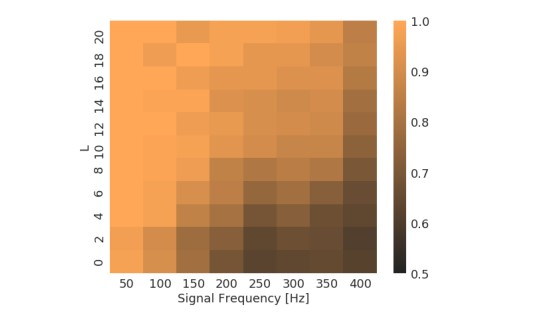
Figure 9. Heatmap of training accuracies of a network trained to predict the binarized value of a sine wave of given frequency (x-axis) defined on for various (y-axis).
图 9. 网络在 上对给定频率(横轴)正弦波的二值化取值做预测时,于不同 (纵轴)下的训练准确率热图。
Observe that increasing (i.e. going up a column in Fig 9) results in better (classification) performance for the same target signal. This is the same behaviour as we observed in Experiment 5 (Fig 8a-d), but now with binary cross-entropy loss instead of the MSE.
可以看到,增大 (即沿图 9 的某一列向上)会使同一目标信号的(分类)表现更好。这与实验 5(图 8a–d)中观察到的行为相同,只是现在用的是二元交叉熵损失,而不是 MSE。
Discussion. These experiments hint towards a rich interaction between the shape of the manifold and the effective difficulty of the learning task. The key mechanism underlying this phenomenon (as we formalize below) is that the relationship between frequency spectrum of the network and that of the fit is mediated by the embedding map . In particular, we argue that a given signal defined on the manifold is easier to fit when the coordinate functions of the manifold embedding itself has high frequency components. Thus, in our experimental setting, the same signal embedded in a flower with more petals can be captured with lower frequencies of the network.
讨论。 这些实验提示,流形的形状与学习任务的有效难度之间存在丰富的相互作用。这一现象背后的关键机制(我们将在下面形式化)是:网络 的频谱与拟合 的频谱之间的关系,由嵌入映射 所中介。具体而言,我们主张:当流形嵌入本身的坐标函数带有高频分量时,定义在该流形上的给定信号会更容易拟合。因此,在我们的实验设置中,同一信号若嵌入花瓣更多的花形曲线,就可以用网络的更低频分量来刻画。
To understand this mathematically, we address the following questions: given a target function , how small can the frequencies of a solution be such that ? And further, how does this relate to the geometry of the data-manifold induced by ? To find out, we write the Fourier transform of the composite function,
为从数学上理解这一点,我们提出如下问题:给定目标函数 ,使 成立的解 ,其频率可以小到什么程度?这又如何与 所诱导的数据流形 的几何有关?为此,我们写出复合函数的傅里叶变换,
The kernel depends on only and elegantly encodes the correspondence between frequencies in input space and frequencies in the latent space . Following a procedure from Bergner et al., we can further investigate the behaviour of the kernel in the regime where the stationary phase approximation is applicable, i.e. when (cf. section 3.2. of Bergner et al.). In this regime, the integral is dominated by critical points of its phase, which satisfy
核 只依赖于 ,并以简洁的方式编码了输入空间中的频率 与潜空间 中的频率 之间的对应。沿用 Bergner et al. 的做法,我们可以进一步考察驻相近似适用的那一区域,也就是 时核的行为(参见 Bergner et al. 第 3.2 节)。在这一区域内,积分 由其相位的临界点 主导,这些临界点满足
where is the Jacobian matrix of . Non-zero values of the kernel correspond to pairs such that Eqn 15 has a solution. Further, given that the components of (i.e. its coordinate functions) are defined on an interval , one can use their Fourier series representation together with Eqn 15 to obtain a condition on their frequencies (shown in appendix C.7). More precisely, we find that the -th component of the RHS in Eqn 15 is proportional to where is the frequency of the coordinate function . This yields that we can get arbitrarily large frequencies if is large enough for large , even when is fixed.
其中 是 的 Jacobi 矩阵。核的非零值对应使式 15 有解的那些对 。进一步,由于 的各个分量(即其坐标函数)定义在区间 上,可以利用它们的傅里叶级数表示,再结合式 15,得到关于其频率的一个条件(见附录 C.7)。更精确地说,我们发现式 15 右端的第 个分量与 成正比,其中 是坐标函数 的频率。由此可得:即便 固定,只要对较大的 , 足够大,就可以得到任意大的频率 。
Consider that the data-domain is bounded, implying that cannot be arbitrarily scaled.
需要考虑到数据定义域是有界的,这意味着 不能被任意缩放。
This is precisely what Experiments 5 and 6 demonstrate in a minimal setting. From Eqn 13, observe that the coordinate functions have a frequency mode at . For increasing , it is apparent that the frequency magnitudes (in the latent space) that can be expressed with the same frequency (in the input space) increases with increasing . This allows the remarkable interpretation that the neural network function can express large frequencies on a manifold () with smaller frequencies w.r.t its input domain (), provided that the coordinate functions of the data manifold embedding itself has high-frequency components.
这正是实验 5 和 6 在一个最小设置中所展示的。由式 13 可见,坐标函数在 处有一个频率模态。随着 增大,用同一输入空间频率 所能表达的潜空间频率幅值 也会随之增大。由此可以得到一个值得注意的解释:只要数据流形嵌入本身的坐标函数带有高频分量,神经网络函数就可以用相对于其输入域更小的频率()来表达流形上的大频率()。
5. Related Work
5. 相关工作
A number of works have focused on showing that neural networks are capable of approximating arbitrarily complex functions. Hornik et al. (1989); Cybenko (1989); Leshno et al. (1993) have shown that neural networks can be universal approximators when given sufficient width; more recently, Lu et al. (2017) proved that this property holds also for width-bounded networks. Montufar et al. (2014) showed that the number of linear regions of deep ReLU networks grows polynomially with width and exponentially with depth; Raghu et al. (2016) generalized this result and provided asymptotically tight bounds. There have been various results of the benefits of depth for efficient approximation (Poole et al., 2016; Telgarsky, 2016; Eldan & Shamir, 2016). These analysis on the expressive power of deep neural networks can in part explain why over-parameterized networks can perfectly learn random input-output mappings (Zhang et al., 2017a).
不少工作致力于表明,神经网络能够逼近任意复杂的函数。Hornik et al. (1989); Cybenko (1989); Leshno et al. (1993) 已经证明,只要宽度足够,神经网络就可以是万能逼近器;更近一些,Lu et al. (2017) 证明宽度有界的网络同样具有这一性质。Montufar et al. (2014) 表明,深度 ReLU 网络的线性区域数目随宽度多项式增长、随深度指数增长;Raghu et al. (2016) 推广了这一结果,并给出了渐近紧的界。关于深度有利于高效逼近,也已有多方面的结果(Poole et al., 2016; Telgarsky, 2016; Eldan & Shamir, 2016)。这些关于深度神经网络表达能力的分析,可以部分解释为何过参数化网络能够完美学习随机的输入–输出映射(Zhang et al., 2017a)。
Our work more directly follows the line of research on implicit regularization in neural networks trained by gradient descent (Neyshabur et al., 2014; Soudry et al., 2017; Poggio et al., 2018; Neyshabur et al., 2017). In fact, while our Fourier analysis of deep ReLU networks also reflects the width and depth dependence of their expressivity, we focused on showing a learning bias of these networks towards simple functions with dominant lower frequency components. We view our results as a first step towards formalizing the findings of Arpit et al. (2017), where it is empirically shown that deep networks prioritize learning simple patterns of the data during training.
我们的工作更直接地延续了关于梯度下降训练神经网络中隐式正则的研究线索(Neyshabur et al., 2014; Soudry et al., 2017; Poggio et al., 2018; Neyshabur et al., 2017)。事实上,尽管我们对深度 ReLU 网络的傅里叶分析也反映出其表达能力对宽度和深度的依赖,但我们把重点放在表明这些网络在学习上偏向以低频分量为主的简单函数。我们把这些结果看作把 Arpit et al. (2017) 的发现形式化的第一步;那篇工作从经验上表明,深度网络在训练中会优先学习数据中的简单模式。
A few other works studied neural networks through the lens of harmonic analysis. For example, Candès (1999) used the ridgelet transform to build constructive procedures for approximating a given function by neural networks, in the case of oscillatory activation functions. This approach has been recently generalized to unbounded activation functions by Sonoda & Murata (2017). Eldan & Shamir (2016) use insights on the support of the Fourier spectrum of two-layer networks to derive a worse-case depth-separation result. Barron (1993) makes use of Fourier space properties of the target function to derive an architecture-dependent approximation bound. In a concurrent and independent work, Xu et al. (2018) make the same observation that lower frequencies are learned first. The subsequent work by Xu (2018) proposes a theoretical analysis of the phenomenon in the case of 2-layer networks with sigmoid activation, based on the spectrum of the sigmoid function.
另有一些工作从调和分析的角度研究神经网络。例如,Candès (1999) 在振荡激活函数的情形下,用 ridgelet 变换构造了用神经网络逼近给定函数的程序。这一方法最近被 Sonoda & Murata (2017) 推广到无界激活函数。Eldan & Shamir (2016) 利用两层网络傅里叶谱支集上的观察,导出了一个最坏情形下的深度分离结果。Barron (1993) 则利用目标函数在傅里叶空间中的性质,给出了依赖于结构的逼近界。在一项同期且独立的工作中,Xu et al. (2018) 也观察到低频会先被学会。随后 Xu (2018) 对带 sigmoid 激活的两层网络提出了该现象的理论分析,依据是 sigmoid 函数的频谱。
In light of our findings, it is worth comparing the case of neural networks and other popular algorithms such that kernel machines (KM) and -nearest neighbor classifiers. We refer to the Appendix E for a detailed discussion and references. In summary, our discussion there suggests that 1. DNNs strike a good balance between function smoothness and expressivity/parameter-efficiency compared with KM; 2. DNNs learn a smoother function compared with NNs since the spectrum of the DNN decays faster compared with NNs in the experiments shown there.
结合我们的发现,值得把神经网络与其他常用算法加以比较,例如核方法(KM)和 近邻分类器。详细讨论与参考文献见附录 E。概括来说,那里的讨论表明:1. 与 KM 相比,DNN 在函数光滑性与表达能力/参数效率之间取得了较好的平衡;2. 与 NN 相比,DNN 学到的函数更光滑,因为在那里给出的实验中,DNN 的频谱比 NN 衰减得更快。
6. Conclusion
6. 结论
We studied deep ReLU networks through the lens of Fourier analysis. Several conclusions can be drawn from our analysis. While neural networks can approximate arbitrary functions, we find that they favour low frequency ones – hence they exhibit a bias towards smooth functions – a phenomenon that we called spectral bias. We also illustrated how the geometry of the data manifold impacts expressivity in a non-trivial way, as high frequency functions defined on complex manifolds can be expressed by lower frequency network functions defined in input space.
我们从傅里叶分析的角度研究了深度 ReLU 网络。分析可以得到若干结论。尽管神经网络能够逼近任意函数,我们发现它们更偏好低频函数——因而表现出对光滑函数的偏向——我们把这一现象称为频谱偏置。我们还说明了数据流形的几何会以并非平凡的方式影响表达能力:定义在复杂流形上的高频函数,可以用定义在输入空间中的更低频网络函数来表达。
We view future work that explore the properties of neural networks in Fourier domain as promising. For example, the Fourier transform affords a natural way of measuring how fast a function can change within a small neighborhood in its input domain; as such, it is a strong candidate for quantifying and analyzing the sensitivity of a model – which in turn provides a natural measure of complexity (Novak et al., 2018). We hope to encourage more research in this direction.
我们认为,今后在傅里叶域中探究神经网络性质的工作是有前景的。例如,傅里叶变换提供了一种自然的方式,来度量一个函数在其输入域的小邻域内可以变化得多快;因此,它是量化和分析模型敏感度的有力候选,而敏感度又给出了一种自然的复杂度度量(Novak et al., 2018)。我们希望能推动这一方向上更多的研究。
Acknowledgements
致谢
The authors would like to thank Ricardo Diaz, Joan Bruna, Rémi Le Priol, Vikram Voleti, Ullrich Köthe, Steffen Wolf, Lorenzo Cerrone, Sebastian Damrich, as well as the anonymous reviewers for their valuable feedback.
作者感谢 Ricardo Diaz、Joan Bruna、Rémi Le Priol、Vikram Voleti、Ullrich Köthe、Steffen Wolf、Lorenzo Cerrone、Sebastian Damrich 以及匿名审稿人提供的宝贵意见。
References
参考文献
Arora, R., Basu, A., Mianjy, P., and Mukherjee, A. Understanding deep neural networks with rectified linear units. In International Conference on Learning Representations, 2018. URL https://openreview.net/forum?id=B1J_rgWRW.
Arpit, D., Jastrzebski, S., Ballas, N., Krueger, D., Bengio, E., Kanwal, M. S., Maharaj, T., Fischer, A., Courville, A., Bengio, Y., et al. A closer look at memorization in deep networks. arXiv preprint arXiv:1706.05394, 2017.
Barron, A. R. Universal approximation bounds for superpositions of a sigmoidal function. IEEE Transactions on Information theory, 39(3):930–945, 1993.
Bengio, Y. et al. Learning deep architectures for ai. Foundations and trends® in Machine Learning, 2(1):1–127, 2009.
Bergner, S., Möller, T., Weiskopf, D., and Muraki, D. J. A spectral analysis of function concatenations and its implications for sampling in direct volume visualization.
Braun, M. L., Lange, T., and Buhmann, J. M. Model selection in kernel methods based on a spectral analysis of label information. In Joint Pattern Recognition Symposium, pp. 344–353. Springer, 2006.
Candès, E. J. Harmonic analysis of neural networks. Applied and Computational Harmonic Analysis, 6(2):197–218, 1999.
Cybenko, G. Approximation by superpositions of a sigmoidal function. Mathematics of Control, Signals, and Systems (MCSS), 2(4):303–314, 1989.
Devroye, L., Györfi, L., and Lugosi, G. Consistency of the k-nearest neighbor rule. In A Probabilistic Theory of Pattern Recognition, pp. 169–185. Springer, 1996.
Diaz, R., Le, Q.-N., and Robins, S. Fourier transforms of polytopes, solid angle sums, and discrete volume. arXiv preprint arXiv:1602.08593, 2016.
Draxler, F., Veschgini, K., Salmhofer, M., and Hamprecht, F. A. Essentially no barriers in neural network energy landscape. arXiv preprint arXiv:1803.00885, 2018.
Eldan, R. and Shamir, O. The power of depth for feedforward neural networks. In Conference on Learning Theory, pp. 907–940, 2016.
Fasshauer, G. E. Positive definite kernels: past, present and future. Dolomite Research Notes on Approximation, 4:21–63, 2011.
Goodfellow, I., Bengio, Y., and Courville, A. Deep Learning. MIT Press, 2016. http://www.deeplearningbook.org.
Goodfellow, I. J., Shlens, J., and Szegedy, C. Explaining and harnessing adversarial examples. arXiv preprint arXiv:1412.6572, 2014.
Hammer, B. and Gersmann, K. A note on the universal approximation capability of support vector machines. Neural Processing Letters, 17(1):43–53, 2003.
Hornik, K., Stinchcombe, M., and White, H. Multilayer feedforward networks are universal approximators. Neural networks, 2(5):359–366, 1989.
Kingma, D. P. and Ba, J. Adam: A method for stochastic optimization. arXiv preprint arXiv:1412.6980, 2014.
Kolsbjerg, E. L., Groves, M. N., and Hammer, B. An automated nudged elastic band method. The Journal of chemical physics, 145(9):094107, 2016.
Leshno, M., Lin, V. Y., Pinkus, A., and Schocken, S. Multilayer feedforward networks with a nonpolynomial activation function can approximate any function. Neural networks, 6(6):861–867, 1993.
Lu, Z., Pu, H., Wang, F., Hu, Z., and Wang, L. The expressive power of neural networks: A view from the width. In Advances in Neural Information Processing Systems, pp. 6231–6239, 2017.
Ma, S. and Belkin, M. Diving into the shallows: a computational perspective on large-scale shallow learning. In Advances in Neural Information Processing Systems, pp. 3781–3790, 2017.
Miyato, T., Kataoka, T., Koyama, M., and Yoshida, Y. Spectral normalization for generative adversarial networks. In International Conference on Learning Representations, 2018. URL https://openreview.net/forum?id=B1QRgziT-.
Montufar, G. F., Pascanu, R., Cho, K., and Bengio, Y. On the number of linear regions of deep neural networks. In Advances in neural information processing systems, pp. 2924–2932, 2014.
Neyshabur, B., Tomioka, R., and Srebro, N. In search of the real inductive bias: On the role of implicit regularization in deep learning. arXiv preprint arXiv:1412.6614, 2014.
Neyshabur, B., Bhojanapalli, S., McAllester, D., and Srebro, N. Exploring generalization in deep learning. In Advances in Neural Information Processing Systems, pp. 5949–5958, 2017.
Novak, R., Bahri, Y., Abolafia, D. A., Pennington, J., and Sohl-Dickstein, J. Sensitivity and generalization in neural networks: an empirical study. In International Conference on Learning Representations, 2018. URL https://openreview.net/forum?id=HJC2SzZCW.
Poggio, T., Kawaguchi, K., Liao, Q., Miranda, B., Rosasco, L., Boix, X., Hidary, J., and Mhaskar, H. Theory of deep learning iii: the non-overfitting puzzle. Technical report, Technical report, CBMM memo 073, 2018.
Poole, B., Lahiri, S., Raghu, M., Sohl-Dickstein, J., and Ganguli, S. Exponential expressivity in deep neural networks through transient chaos. In Lee, D. D., Sugiyama, M., Luxburg, U. V., Guyon, I., and Garnett, R. (eds.), Advances in Neural Information Processing Systems 29, pp. 3360–3368. Curran Associates, Inc., 2016.
Raghu, M., Poole, B., Kleinberg, J., Ganguli, S., and Sohl-Dickstein, J. On the expressive power of deep neural networks. arXiv preprint arXiv:1606.05336, 2016.
Rasmussen, C. E. Gaussian processes in machine learning. In Advanced lectures on machine learning, pp. 63–71. Springer, 2004.
Serov, V. Fourier series, Fourier transform and their applications to mathematical physics. Springer, 2017.
Sonoda, S. and Murata, N. Neural network with unbounded activation functions is universal approximator. Applied and Computational Harmonic Analysis, 43(2):233–268, 2017.
Soudry, D., Hoffer, E., Nacson, M. S., Gunasekar, S., and Srebro, N. The implicit bias of gradient descent on separable data. arXiv preprint arXiv:1710.10345, 2017.
Spivak, M. Calculus On Manifolds: A Modern Approach To Classical Theorems Of Advanced Calculus. CRC press, 2018.
Telgarsky, M. Benefits of depth in neural networks. Conference on Learning Theory (COLT), 2016, 2016.
Xu, Z. J. Understanding training and generalization in deep learning by fourier analysis. arXiv preprint arXiv:1808.04295, 2018.
Xu, Z.-Q. J., Zhang, Y., and Xiao, Y. Training behavior of deep neural network in frequency domain. arXiv preprint arXiv:1807.01251, 2018.
Zhang, C., Bengio, S., Hardt, M., Recht, B., and Vinyals, O. Understanding deep learning requires rethinking generalization. International Conference on Learning Representations (ICLR), 2017a.
Zhang, H., Cisse, M., Dauphin, Y. N., and Lopez-Paz, D. mixup: Beyond empirical risk minimization. arXiv preprint arXiv:1710.09412, 2017b.
Zhang, L., Naitzat, G., and Lim, L.-H. Tropical geometry of deep neural networks. arXiv preprint arXiv:1805.07091, 2018.