Spatial Transformer Networks
Spatial Transformer Networks
Abstract
Convolutional Neural Networks define an exceptionally powerful class of models, but are still limited by the lack of ability to be spatially invariant to the input data in a computationally and parameter efficient manner. In this work we introduce a new learnable module, the Spatial Transformer, which explicitly allows the spatial manipulation of data within the network. This differentiable module can be inserted into existing convolutional architectures, giving neural networks the ability to actively spatially transform feature maps, conditional on the feature map itself, without any extra training supervision or modification to the optimisation process. We show that the use of spatial transformers results in models which learn invariance to translation, scale, rotation and more generic warping, resulting in state-of-the-art performance on several benchmarks, and for a number of classes of transformations.
卷积神经网络是一类能力很强的模型,但仍然缺少一种计算上和参数上都高效的办法,使模型对输入的空间变化保持不变。本文提出一种新的可学习模块,即空间变换器(Spatial Transformer),它明确允许在网络内部对数据做空间操作。这个可微模块可以插入已有的卷积结构,使神经网络能够依据特征图自身,主动地对特征图做空间变换,无需额外的训练监督,也不必改动优化过程。我们表明,使用空间变换器后,模型可以学到对平移、缩放、旋转以及更一般的扭曲的不变性,并在多个基准以及多种变换类别上达到当时最好成绩。
1 Introduction
Over recent years, the landscape of computer vision has been drastically altered and pushed forward through the adoption of a fast, scalable, end-to-end learning framework, the Convolutional Neural Network (CNN) [18]. Though not a recent invention, we now see a cornucopia of CNN-based models achieving state-of-the-art results in classification, localisation, semantic segmentation, and action recognition tasks, amongst others.
近年来,计算机视觉的面貌被一种快速、可扩展、端到端的学习框架大幅改写并向前推进,这就是卷积神经网络(CNN)[18]。它并不是新发明,但我们现在已经看到大量基于 CNN 的模型,在分类、定位、语义分割和动作识别等任务上取得当时最好成绩。
A desirable property of a system which is able to reason about images is to disentangle object pose and part deformation from texture and shape. The introduction of local max-pooling layers in CNNs has helped to satisfy this property by allowing a network to be somewhat spatially invariant to the position of features. However, due to the typically small spatial support for max-pooling (e.g. pixels) this spatial invariance is only realised over a deep hierarchy of max-pooling and convolutions, and the intermediate feature maps (convolutional layer activations) in a CNN are not actually invariant to large transformations of the input data [5, 19]. This limitation of CNNs is due to having only a limited, pre-defined pooling mechanism for dealing with variations in the spatial arrangement of data.
一个能够对图像做推理的系统,最好能把物体的姿态和部件形变,从纹理与形状中分离出来。CNN 中引入的局部最大池化层,让网络对特征的位置具有一定的空间不变性,从而有助于满足这一性质。不过,最大池化的空间支持通常很小(例如 像素),这种不变性只有经过很深的一层层池化与卷积才会体现出来,而 CNN 的中间特征图(卷积层激活)实际上并不能对输入的大幅变换保持不变 [5, 19]。CNN 的这一局限,来自它只能依靠一种有限且预先设定的池化机制,来处理数据空间排布上的变化。
In this work we introduce the Spatial Transformer module, that can be included into a standard neural network architecture to provide spatial transformation capabilities. The action of the spatial transformer is conditioned on individual data samples, with the appropriate behaviour learnt during training for the task in question (without extra supervision). Unlike pooling layers, where the receptive fields are fixed and local, the spatial transformer module is a dynamic mechanism that can actively spatially transform an image (or a feature map) by producing an appropriate transformation for each input sample. The transformation is then performed on the entire feature map (non-locally) and can include scaling, cropping, rotations, as well as non-rigid deformations. This allows networks which include spatial transformers to not only select regions of an image that are most relevant (attention), but also to transform those regions to a canonical, expected pose to simplify inference in the subsequent layers. Notably, spatial transformers can be trained with standard back-propagation, allowing for end-to-end training of the models they are injected in.
本文提出空间变换器(Spatial Transformer)模块,它可以加入标准神经网络结构,为网络提供空间变换能力。空间变换器的行为以单个数据样本为条件,在训练中针对当前任务学到合适的表现,无需额外监督。与感受野固定且局部的池化层不同,空间变换器是一种动态机制:它为每个输入样本生成合适的变换,从而主动地对图像或特征图做空间变换。变换作用于整张特征图(非局部),可以包括缩放、裁剪、旋转以及非刚性形变。因此,带有空间变换器的网络不仅可以选出图像中最相关的区域(注意力),还可以把这些区域变换到一种规范、预期的姿态,从而简化后续层的推理。值得指出的是,空间变换器可以用标准反向传播训练,从而对其所插入的模型做端到端训练。
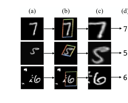
Figure 1: The result of using a spatial transformer as the first layer of a fully-connected network trained for distorted MNIST digit classification. (a) The input to the spatial transformer network is an image of an MNIST digit that is distorted with random translation, scale, rotation, and clutter. (b) The localisation network of the spatial transformer predicts a transformation to apply to the input image. (c) The output of the spatial transformer, after applying the transformation. (d) The classification prediction produced by the subsequent fully-connected network on the output of the spatial transformer. The spatial transformer network (a CNN including a spatial transformer module) is trained end-to-end with only class labels – no knowledge of the groundtruth transformations is given to the system.
图 1:把空间变换器作为全连接网络的第一层,用于扭曲 MNIST 数字分类的结果。(a) 空间变换器网络的输入是一张经过随机平移、缩放、旋转和杂乱背景干扰的 MNIST 数字图像。(b) 空间变换器的定位网络预测应对输入图像施加的变换。(c) 施加变换后,空间变换器的输出。(d) 后续全连接网络在空间变换器输出上给出的分类预测。该空间变换器网络(即包含空间变换器模块的 CNN)只使用类别标签做端到端训练,系统并不知道真实变换。
Spatial transformers can be incorporated into CNNs to benefit multifarious tasks, for example: (i) image classification: suppose a CNN is trained to perform multi-way classification of images according to whether they contain a particular digit – where the position and size of the digit may vary significantly with each sample (and are uncorrelated with the class); a spatial transformer that crops out and scale-normalizes the appropriate region can simplify the subsequent classification task, and lead to superior classification performance, see Fig. 1; (ii) co-localisation: given a set of images containing different instances of the same (but unknown) class, a spatial transformer can be used to localise them in each image; (iii) spatial attention: a spatial transformer can be used for tasks requiring an attention mechanism, such as in [11, 29], but is more flexible and can be trained purely with backpropagation without reinforcement learning. A key benefit of using attention is that transformed (and so attended), lower resolution inputs can be used in favour of higher resolution raw inputs, resulting in increased computational efficiency.
空间变换器可以并入 CNN,使多种任务受益,例如:(i) 图像分类:假设 CNN 要按图像中是否包含某个数字做多路分类,而数字的位置和大小在各个样本上可能变化很大,且与类别无关;一个能够裁出相应区域并做尺度归一化的空间变换器,可以简化后续分类,并带来更好的分类表现,见图 1;(ii) 协同定位:给定一组图像,其中包含同一(但未知)类别的不同实例,可以用空间变换器在每张图中把它们定位出来;(iii) 空间注意力:空间变换器也可用于需要注意力机制的任务,如 [11, 29],但更灵活,并且可以只用反向传播训练,不必借助强化学习。使用注意力的一个关键好处是,可以用经过变换(因而被关注到)、分辨率更低的输入,来代替更高分辨率的原始输入,从而提高计算效率。
The rest of the paper is organised as follows: Sect. 2 discusses some work related to our own, we introduce the formulation and implementation of the spatial transformer in Sect. 3, and finally give the results of experiments in Sect. 4. Additional experiments and implementation details are given in the supplementary material or can be found in the arXiv version.
本文其余部分组织如下:第 2 节讨论与本文相关的一些工作,第 3 节给出空间变换器的形式化与实现,第 4 节给出实验结果。更多实验与实现细节见补充材料,也可在 arXiv 版本中找到。
2 Related Work
In this section we discuss the prior work related to the paper, covering the central ideas of modelling transformations with neural networks [12, 13, 27], learning and analysing transformation-invariant representations [3, 5, 8, 17, 19, 25], as well as attention and detection mechanisms for feature selection [1, 6, 9, 11, 23].
本节讨论与本文相关的已有工作,涵盖用神经网络对变换建模的核心思路 [12, 13, 27],学习并分析变换不变表示 [3, 5, 8, 17, 19, 25],以及用于特征选择的注意力与检测机制 [1, 6, 9, 11, 23]。
Early work by Hinton [12] looked at assigning canonical frames of reference to object parts, a theme which recurred in [13] where 2D affine transformations were modeled to create a generative model composed of transformed parts. The targets of the generative training scheme are the transformed input images, with the transformations between input images and targets given as an additional input to the network. The result is a generative model which can learn to generate transformed images of objects by composing parts. The notion of a composition of transformed parts is taken further by Tieleman [27], where learnt parts are explicitly affine-transformed, with the transform predicted by the network. Such generative capsule models are able to learn discriminative features for classification from transformation supervision.
Hinton 的早期工作 [12] 考虑为物体部件指定规范参考系,这一主题在 [13] 中再次出现:那里对二维仿射变换建模,以构造由变换后的部件组成的生成模型。生成式训练的目标是变换后的输入图像,输入图像与目标之间的变换作为额外输入送给网络。得到的生成模型可以通过组合部件,学会生成物体的变换图像。Tieleman [27] 把“变换部件的组合”这一想法又推进了一步:学到的部件被显式地做仿射变换,变换由网络预测。这类生成式胶囊模型能够在变换监督下,学到用于分类的判别特征。
The invariance and equivariance of CNN representations to input image transformations are studied in [19] by estimating the linear relationships between representations of the original and transformed images. Cohen & Welling [5] analyse this behaviour in relation to symmetry groups, which is also exploited in the architecture proposed by Gens & Domingos [8], resulting in feature maps that are more invariant to symmetry groups. Other attempts to design transformation invariant representations are scattering networks [3], and CNNs that construct filter banks of transformed filters [17, 25]. Stollenga et al. [26] use a policy based on a network’s activations to gate the responses of the network’s filters for a subsequent forward pass of the same image and so can allow attention to specific features. In this work, we aim to achieve invariant representations by manipulating the data rather than the feature extractors, something that was done for clustering in [7].
[19] 通过估计原图表示与变换图像表示之间的线性关系,研究了 CNN 表示对输入图像变换的不变性与等变性。Cohen 和 Welling [5] 从对称群的角度分析了这一行为;Gens 和 Domingos [8] 提出的结构也利用了这一点,从而得到对对称群更加不变的特征图。其他设计变换不变表示的尝试还包括散射网络 [3],以及用变换后的滤波器构造滤波器组的 CNN [17, 25]。Stollenga 等人 [26] 根据网络激活得到一项策略,用来在同一张图像的下一次前向中门控滤波器响应,从而可以把注意力放到特定特征上。在本文中,我们希望通过操纵数据而不是特征提取器,来获得不变表示;类似做法曾用于聚类 [7]。
Neural networks with selective attention manipulate the data by taking crops, and so are able to learn translation invariance. Work such as [1, 23] are trained with reinforcement learning to avoid the need for a differentiable attention mechanism, while [11] use a differentiable attention mechansim by utilising Gaussian kernels in a generative model. The work by Girshick et al. [9] uses a region proposal algorithm as a form of attention, and [6] show that it is possible to regress salient regions with a CNN. The framework we present in this paper can be seen as a generalisation of differentiable attention to any spatial transformation.
带有选择性注意力的神经网络通过裁剪来操纵数据,因而能够学习平移不变性。[1, 23] 等工作用强化学习训练,以避免需要可微的注意力机制;而 [11] 在生成模型中利用高斯核,采用了一种可微的注意力机制。Girshick 等人 [9] 把区域提议算法当作一种注意力,[6] 则表明可以用 CNN 回归出显著区域。本文给出的框架,可以看作把可微注意力推广到任意空间变换。
3 Spatial Transformers
In this section we describe the formulation of a spatial transformer. This is a differentiable module which applies a spatial transformation to a feature map during a single forward pass, where the transformation is conditioned on the particular input, producing a single output feature map. For multi-channel inputs, the same warping is applied to each channel. For simplicity, in this section we consider single transforms and single outputs per transformer, however we can generalise to multiple transformations, as shown in experiments.
本节给出空间变换器的形式化描述。它是一个可微模块,在一次前向过程中对特征图施加空间变换;变换以当前输入为条件,并产生一张输出特征图。对多通道输入,同一套扭曲会施加到每个通道上。为简明起见,本节先考虑每个变换器只有一次变换、一张输出的情形;不过也可以推广到多次变换,实验中会给出。
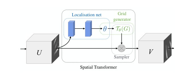
Figure 2: The architecture of a spatial transformer module. The input feature map is passed to a localisation network which regresses the transformation parameters . The regular spatial grid over is transformed to the sampling grid , which is applied to as described in Sect. 3.3, producing the warped output feature map . The combination of the localisation network and sampling mechanism defines a spatial transformer.
图 2:空间变换器模块的结构。输入特征图 被送入定位网络,由它回归出变换参数 。输出 上的规则空间网格 被变换成采样网格 ,再按第 3.3 节所述作用于 ,得到扭曲后的输出特征图 。定位网络与采样机制合在一起,就定义了一个空间变换器。
The spatial transformer mechanism is split into three parts, shown in Fig. 2. In order of computation, first a localisation network (Sect. 3.1) takes the input feature map, and through a number of hidden layers outputs the parameters of the spatial transformation that should be applied to the feature map – this gives a transformation conditional on the input. Then, the predicted transformation parameters are used to create a sampling grid, which is a set of points where the input map should be sampled to produce the transformed output. This is done by the grid generator, described in Sect. 3.2. Finally, the feature map and the sampling grid are taken as inputs to the sampler, producing the output map sampled from the input at the grid points (Sect. 3.3).
空间变换器机制分成三个部分,见图 2。按计算顺序,首先由定位网络(第 3.1 节)接收输入特征图,经过若干隐层,输出应对该特征图施加的空间变换参数——这样就得到了以输入为条件的变换。随后,用预测出的变换参数生成采样网格,也就是为得到变换后的输出而应在输入图上取样的一组点。这一步由第 3.2 节所述的网格生成器完成。最后,特征图和采样网格被送入采样器,在网格点处从输入取样,得到输出特征图(第 3.3 节)。
The combination of these three components forms a spatial transformer and will now be described in more detail in the following sections.
这三个部件合在一起,就构成一个空间变换器。下面各节再分别细述。
3.1 Localisation Network
The localisation network takes the input feature map with width , height and channels and outputs , the parameters of the transformation to be applied to the feature map: . The size of can vary depending on the transformation type that is parameterised, e.g. for an affine transformation is 6-dimensional as in (1).
定位网络接收宽为 、高为 、通道数为 的输入特征图 ,并输出应对该特征图施加的变换 的参数 :。 的维数随所参数化的变换类型而变化,例如对仿射变换, 如 (1) 所示是 6 维的。
The localisation network function can take any form, such as a fully-connected network or a convolutional network, but should include a final regression layer to produce the transformation parameters .
定位网络函数 可以取任意形式,例如全连接网络或卷积网络,但应包含一个最终的回归层,以产生变换参数 。
3.2 Parameterised Sampling Grid
To perform a warping of the input feature map, each output pixel is computed by applying a sampling kernel centered at a particular location in the input feature map (this is described fully in the next section). By pixel we refer to an element of a generic feature map, not necessarily an image. In general, the output pixels are defined to lie on a regular grid of pixels , forming an output feature map , where and are the height and width of the grid, and is the number of channels, which is the same in the input and output.
要对输入特征图做扭曲,每个输出像素都是通过在输入特征图的某个位置为中心施加采样核来计算的(下一节将完整说明)。这里所说的像素,泛指一般特征图中的一个元素,不必是图像像素。一般地,输出像素被定义在规则网格 上,其中 ,从而形成输出特征图 。 和 是网格的高度和宽度, 是通道数,与输入、输出相同。
For clarity of exposition, assume for the moment that is a 2D affine transformation . We will discuss other transformations below. In this affine case, the pointwise transformation is
为表述清楚,暂时假定 是二维仿射变换 。其他变换稍后再讨论。在这种仿射情形下,逐点变换为
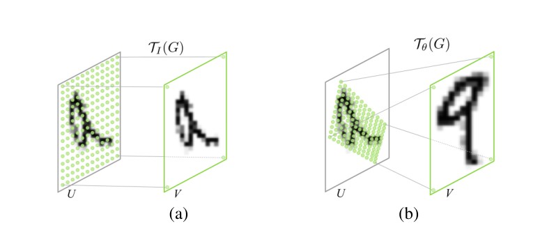
Figure 3: Two examples of applying the parameterised sampling grid to an image producing the output . (a) The sampling grid is the regular grid , where is the identity transformation parameters. (b) The sampling grid is the result of warping the regular grid with an affine transformation .
图 3:把参数化采样网格施加到图像 上、得到输出 的两个例子。(a) 采样网格就是规则网格 ,其中 是恒等变换参数。(b) 采样网格是用仿射变换 把规则网格扭曲后的结果。
where are the target coordinates of the regular grid in the output feature map, are the source coordinates in the input feature map that define the sample points, and is the affine transformation matrix. We use height and width normalised coordinates, such that when within the spatial bounds of the output, and when within the spatial bounds of the input (and similarly for the coordinates). The source/target transformation and sampling is equivalent to the standard texture mapping and coordinates used in graphics.
其中 是输出特征图中规则网格的目标坐标, 是输入特征图中定义采样点的源坐标, 是仿射变换矩阵。我们使用按高度和宽度归一化的坐标:当点落在输出的空间范围内时,;当点落在输入的空间范围内时,( 坐标同样如此)。这种源/目标变换与采样,等价于图形学中常用的纹理映射及其坐标。
The transform defined in (1) allows cropping, translation, rotation, scale, and skew to be applied to the input feature map, and requires only 6 parameters (the 6 elements of ) to be produced by the localisation network. It allows cropping because if the transformation is a contraction (i.e. the determinant of the left sub-matrix has magnitude less than unity) then the mapped regular grid will lie in a parallelogram of area less than the range of . The effect of this transformation on the grid compared to the identity transform is shown in Fig. 3.
(1) 中定义的变换可以对输入特征图做裁剪、平移、旋转、缩放和错切,定位网络只需产生 6 个参数(即 的 6 个元素)。它之所以能做裁剪,是因为若变换是收缩(即左侧 子矩阵的行列式绝对值小于 1),则映射后的规则网格会落在一块面积小于 取值范围的平行四边形内。与恒等变换相比,这一变换对网格的影响见图 3。
The class of transformations may be more constrained, such as that used for attention
变换类 也可以更受约束,例如用于注意力的那种
allowing cropping, translation, and isotropic scaling by varying , , and . The transformation can also be more general, such as a plane projective transformation with 8 parameters, piecewise affine, or a thin plate spline. Indeed, the transformation can have any parameterised form, provided that it is differentiable with respect to the parameters – this crucially allows gradients to be backpropagated through from the sample points to the localisation network output . If the transformation is parameterised in a structured, low-dimensional way, this reduces the complexity of the task assigned to the localisation network. For instance, a generic class of structured and differentiable transformations, which is a superset of attention, affine, projective, and thin plate spline transformations, is , where is a target grid representation (e.g. in (1), is the regular grid in homogeneous coordinates), and is a matrix parameterised by . In this case it is possible to not only learn how to predict for a sample, but also to learn for the task at hand.
通过改变 、 和 ,就可以做裁剪、平移和各向同性缩放。变换 也可以更一般,例如 8 参数的平面投影变换、分片仿射,或薄板样条。事实上,只要变换对参数可微,它就可以取任意参数化形式——这一点至关重要,因为它允许梯度从采样点 反向传播到定位网络的输出 。若变换以结构化、低维的方式参数化,定位网络所承担任务的复杂度就会降低。例如,一类通用的结构化可微变换(它是注意力、仿射、投影和薄板样条变换的超集)可写成 ,其中 是目标网格表示(例如在 (1) 中, 是齐次坐标下的规则网格 ), 是由 参数化的矩阵。此时不仅可以学习如何为某个样本预测 ,还可以为当前任务学习 。
3.3 Differentiable Image Sampling
To perform a spatial transformation of the input feature map, a sampler must take the set of sampling points , along with the input feature map and produce the sampled output feature map .
要对输入特征图做空间变换,采样器必须接收采样点集合 以及输入特征图 ,并产生采样后的输出特征图 。
Each coordinate in defines the spatial location in the input where a sampling kernel is applied to get the value at a particular pixel in the output . This can be written as
中的每个坐标 给出了输入中施加采样核的空间位置,从而得到输出 中某一像素的取值。它可以写成
where and are the parameters of a generic sampling kernel which defines the image interpolation (e.g. bilinear), is the value at location in channel of the input, and is the output value for pixel at location in channel . Note that the sampling is done identically for each channel of the input, so every channel is transformed in an identical way (this preserves spatial consistency between channels).
其中 和 是通用采样核 的参数,该核定义了图像插值方式(例如双线性); 是输入第 通道在位置 处的值, 是第 通道中位于 的输出像素 的值。注意,采样对输入的每个通道都以相同方式进行,因此所有通道都以相同方式被变换(这保持了通道之间的空间一致性)。
In theory, any sampling kernel can be used, as long as (sub-)gradients can be defined with respect to and . For example, using the integer sampling kernel reduces (3) to
理论上可以使用任意采样核,只要能够对 和 定义(次)梯度。例如,使用整数采样核时,(3) 就化为
where rounds to the nearest integer and is the Kronecker delta function. This sampling kernel equates to just copying the value at the nearest pixel to to the output location . Alternatively, a bilinear sampling kernel can be used, giving
其中 把 四舍五入到最近整数, 是克罗内克函数。这个采样核等价于把最靠近 的像素值复制到输出位置 。也可以改用双线性采样核,得到
To allow backpropagation of the loss through this sampling mechanism we can define the gradients with respect to and . For bilinear sampling (5) the partial derivatives are
为了让损失能够通过这一采样机制反向传播,我们可以定义对 和 的梯度。对双线性采样 (5),偏导数为
and similarly to (7) for .
对 也可类似地按 (7) 写出。
This gives us a (sub-)differentiable sampling mechanism, allowing loss gradients to flow back not only to the input feature map (6), but also to the sampling grid coordinates (7), and therefore back to the transformation parameters and localisation network since and can be easily derived from (1) for example. Due to discontinuities in the sampling fuctions, sub-gradients must be used. This sampling mechanism can be implemented very efficiently on GPU, by ignoring the sum over all input locations and instead just looking at the kernel support region for each output pixel.
这就得到了一种(次)可微的采样机制,使损失梯度不仅可以回到输入特征图 (6),也可以回到采样网格坐标 (7),进而回到变换参数 和定位网络,因为例如 和 可以由 (1) 容易地导出。由于采样函数中存在间断,必须使用次梯度。这一采样机制可以在 GPU 上实现得非常高效:不必对所有输入位置求和,只需考察每个输出像素的核支撑区域。
3.4 Spatial Transformer Networks
The combination of the localisation network, grid generator, and sampler form a spatial transformer (Fig. 2). This is a self-contained module which can be dropped into a CNN architecture at any point, and in any number, giving rise to spatial transformer networks. This module is computationally very fast and does not impair the training speed, causing very little time overhead when used naively, and even potential speedups in attentive models due to subsequent downsampling that can be applied to the output of the transformer.
定位网络、网格生成器和采样器合在一起,就构成一个空间变换器(图 2)。这是一个自包含模块,可以在 CNN 结构的任意位置、以任意数量插入,从而形成空间变换器网络。该模块计算上非常快,不会拖慢训练:即使不加特别优化,时间开销也很小;在注意力式模型中,还可以对变换器输出再做降采样,因而甚至有可能加快速度。
Placing spatial transformers within a CNN allows the network to learn how to actively transform the feature maps to help minimise the overall cost function of the network during training. The knowledge of how to transform each training sample is compressed and cached in the weights of the localisation network (and also the weights of the layers previous to a spatial transformer) during training. For some tasks, it may also be useful to feed the output of the localisation network, , forward to the rest of the network, as it explicitly encodes the transformation, and hence the pose, of a region or object.
把空间变换器放进 CNN,可以让网络在训练中学会主动变换特征图,以帮助最小化网络的总体代价函数。如何变换每个训练样本的知识,会在训练过程中被压缩并缓存在定位网络的权重里(以及空间变换器之前各层的权重里)。对某些任务,把定位网络的输出 再向前送给网络的其余部分也可能有用,因为它显式编码了某个区域或物体的变换,从而也就编码了其姿态。
It is also possible to use spatial transformers to downsample or oversample a feature map, as one can define the output dimensions and to be different to the input dimensions and . However, with sampling kernels with a fixed, small spatial support (such as the bilinear kernel), downsampling with a spatial transformer can cause aliasing effects.
也可以用空间变换器对特征图做降采样或过采样,因为可以把输出尺寸 和 定义成与输入尺寸 和 不同。不过,若采样核的空间支撑固定且较小(例如双线性核),用空间变换器做降采样可能产生混叠。
Finally, it is possible to have multiple spatial transformers in a CNN. Placing multiple spatial transformers at increasing depths of a network allow transformations of increasingly abstract representations, and also gives the localisation networks potentially more informative representations to base the predicted transformation parameters on. One can also use multiple spatial transformers in parallel – this can be useful if there are multiple objects or parts of interest in a feature map that should be focussed on individually. A limitation of this architecture in a purely feed-forward network is that the number of parallel spatial transformers limits the number of objects that the network can model.
最后,CNN 中也可以放置多个空间变换器。把多个空间变换器放在网络越来越深的位置,就可以对越来越抽象的表示做变换,同时也让定位网络有可能依据信息更丰富的表示来预测变换参数。还可以并行使用多个空间变换器——如果特征图中有多个需要分别关注的物体或部件,这就很有用。在纯前馈网络中,这一结构的一个局限是:并行空间变换器的数量,限制了网络能够建模的物体数量。
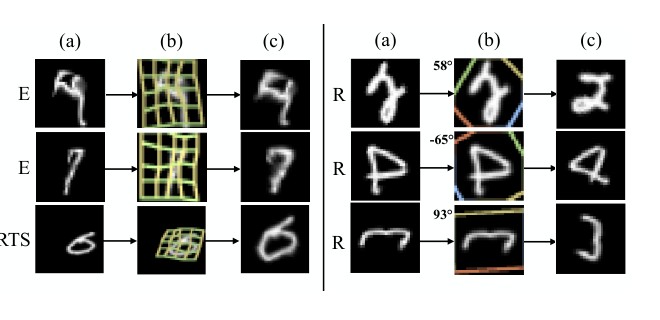
Table 1: Left: The percentage errors for different models on different distorted MNIST datasets. The different distorted MNIST datasets we test are TC: translated and cluttered, R: rotated, RTS: rotated, translated, and scaled, P: projective distortion, E: elastic distortion. All the models used for each experiment have the same number of parameters, and same base structure for all experiments. Right: Some example test images where a spatial transformer network correctly classifies the digit but a CNN fails. (a) The inputs to the networks. (b) The transformations predicted by the spatial transformers, visualised by the grid . (c) The outputs of the spatial transformers. E and RTS examples use thin plate spline spatial transformers (ST-CNN TPS), while R examples use affine spatial transformers (ST-CNN Aff) with the angles of the affine transformations given. For videos showing animations of these experiments and more see https://goo.gl/qdEhUu.
| Model | R | RTS | P | E | |
|---|---|---|---|---|---|
| FCN | 2.1 | 5.2 | 3.1 | 3.2 | |
| CNN | 1.2 | 0.8 | 1.5 | 1.4 | |
| ST-FCN | Aff | 1.2 | 0.8 | 1.5 | 2.7 |
| ST-FCN | Proj | 1.3 | 0.9 | 1.4 | 2.6 |
| ST-FCN | TPS | 1.1 | 0.8 | 1.4 | 2.4 |
| ST-CNN | Aff | 0.7 | 0.5 | 0.8 | 1.2 |
| ST-CNN | Proj | 0.8 | 0.6 | 0.8 | 1.3 |
| ST-CNN | TPS | 0.7 | 0.5 | 0.8 | 1.1 |
图为表 1 右侧的可视化。表 1:左:不同模型在不同扭曲 MNIST 数据集上的误差百分比。我们测试的不同扭曲 MNIST 数据集为 TC:平移并加杂乱背景,R:旋转,RTS:旋转、平移并缩放,P:投影扭曲,E:弹性扭曲。每个实验所用的全部模型参数量相同,且所有实验的基础结构相同。右:一些测试图像的例子,空间变换器网络能正确分类数字,而 CNN 不能。(a) 网络的输入。(b) 空间变换器预测的变换,用网格 可视化。(c) 空间变换器的输出。E 和 RTS 的例子使用薄板样条空间变换器(ST-CNN TPS),R 的例子使用仿射空间变换器(ST-CNN Aff),并给出仿射变换的角度。展示这些实验动画及更多内容的视频见 https://goo.gl/qdEhUu。
| 模型 | R | RTS | P | E | |
|---|---|---|---|---|---|
| FCN | 2.1 | 5.2 | 3.1 | 3.2 | |
| CNN | 1.2 | 0.8 | 1.5 | 1.4 | |
| ST-FCN | Aff | 1.2 | 0.8 | 1.5 | 2.7 |
| ST-FCN | Proj | 1.3 | 0.9 | 1.4 | 2.6 |
| ST-FCN | TPS | 1.1 | 0.8 | 1.4 | 2.4 |
| ST-CNN | Aff | 0.7 | 0.5 | 0.8 | 1.2 |
| ST-CNN | Proj | 0.8 | 0.6 | 0.8 | 1.3 |
| ST-CNN | TPS | 0.7 | 0.5 | 0.8 | 1.1 |
4 Experiments
In this section we explore the use of spatial transformer networks on a number of supervised learning tasks. In Sect. 4.1 we begin with experiments on distorted versions of the MNIST handwriting dataset, showing the ability of spatial transformers to improve classification performance through actively transforming the input images. In Sect. 4.2 we test spatial transformer networks on a challenging real-world dataset, Street View House Numbers [21], for number recognition, showing state-of-the-art results using multiple spatial transformers embedded in the convolutional stack of a CNN. Finally, in Sect. 4.3, we investigate the use of multiple parallel spatial transformers for fine-grained classification, showing state-of-the-art performance on CUB-200-2011 birds dataset [28] by automatically discovering object parts and learning to attend to them. Further experiments with MNIST addition and co-localisation can be found in the supplementary material.
本节在若干有监督学习任务上考察空间变换器网络的使用。第 4.1 节首先在扭曲版 MNIST 手写数据集上做实验,说明空间变换器能够通过主动变换输入图像来提高分类表现。第 4.2 节在具有挑战性的真实世界数据集 Street View House Numbers [21] 上测试空间变换器网络,用于数字识别,把多个空间变换器嵌入 CNN 的卷积堆叠后达到当时最好结果。最后,第 4.3 节研究并行使用多个空间变换器做细粒度分类,通过自动发现物体部件并学会关注它们,在 CUB-200-2011 鸟类数据集 [28] 上达到当时最好成绩。关于 MNIST 加法和协同定位的更多实验见补充材料。
4.1 Distorted MNIST
In this section we use the MNIST handwriting dataset as a testbed for exploring the range of transformations to which a network can learn invariance to by using a spatial transformer.
本节把 MNIST 手写数据集当作试验台,用来考察网络借助空间变换器能够学到对哪些范围的变换保持不变。
We begin with experiments where we train different neural network models to classify MNIST data that has been distorted in various ways: rotation (R); rotation, scale and translation (RTS); projective transformation (P); elastic warping (E) – note that elastic warping is destructive and cannot be inverted in some cases. The full details of the distortions used to generate this data are given in the supplementary material. We train baseline fully-connected (FCN) and convolutional (CNN) neural networks, as well as networks with spatial transformers acting on the input before the classification network (ST-FCN and ST-CNN). The spatial transformer networks all use bilinear sampling, but variants use different transformation functions: an affine transformation (Aff), projective transformation (Proj), and a 16-point thin plate spline transformation (TPS) with a regular grid of control points. The CNN models include two max-pooling layers. All networks have approximately the same number of parameters, are trained with identical optimisation schemes (backpropagation, SGD, scheduled learning rate decrease, with a multinomial cross entropy loss), and all with three weight layers in the classification network.
我们先做一组实验:训练不同的神经网络模型,对以各种方式扭曲过的 MNIST 数据做分类:旋转(R);旋转、缩放和平移(RTS);投影变换(P);弹性扭曲(E)——需要注意,弹性扭曲具有破坏性,有时无法求逆。生成这些数据所用扭曲的完整细节见补充材料。我们训练基线全连接网络(FCN)和卷积网络(CNN),以及在分类网络之前对输入作用空间变换器的网络(ST-FCN 和 ST-CNN)。这些空间变换器网络都使用双线性采样,但不同变体使用不同的变换函数:仿射变换(Aff)、投影变换(Proj),以及控制点落在规则网格上的 16 点薄板样条变换(TPS)。CNN 模型包含两个最大池化层。所有网络的参数量大致相同,用同一套优化方案训练(反向传播、SGD、按计划降低学习率,损失为多项交叉熵),并且分类网络都有三层带权重的层。
The results of these experiments are shown in Table 1 (left). Looking at any particular type of distortion of the data, it is clear that a spatial transformer enabled network outperforms its counterpart base network. For the case of rotation, translation, and scale distortion (RTS), the ST-CNN achieves 0.5% and 0.6% depending on the class of transform used for , whereas a CNN, with two max-pooling layers to provide spatial invariance, achieves 0.8% error. This is in fact the same error that the ST-FCN achieves, which is without a single convolution or max-pooling layer in its network, showing that using a spatial transformer is an alternative way to achieve spatial invariance. ST-CNN models consistently perform better than ST-FCN models due to max-pooling layers in ST-CNN providing even more spatial invariance, and convolutional layers better modelling local structure. We also test our models in a noisy environment, on images with translated MNIST digits and
这些实验的结果见表 1(左)。就数据的任意一种扭曲类型来看,带有空间变换器的网络都明显好于对应的基线网络。在旋转、平移和缩放扭曲(RTS)的情形下,ST-CNN 依 所用变换类别的不同,分别达到 0.5% 和 0.6%,而靠两个最大池化层提供空间不变性的 CNN 误差为 0.8%。这实际上与 ST-FCN 的误差相同,而 ST-FCN 的网络里没有任何卷积或最大池化层,说明使用空间变换器是获得空间不变性的另一条途径。ST-CNN 模型始终好于 ST-FCN 模型,因为 ST-CNN 中的最大池化层提供了更多空间不变性,卷积层也更能刻画局部结构。我们还在带噪声的环境中测试了这些模型,使用的是 图像,其中是经过平移的 MNIST 数字,并且
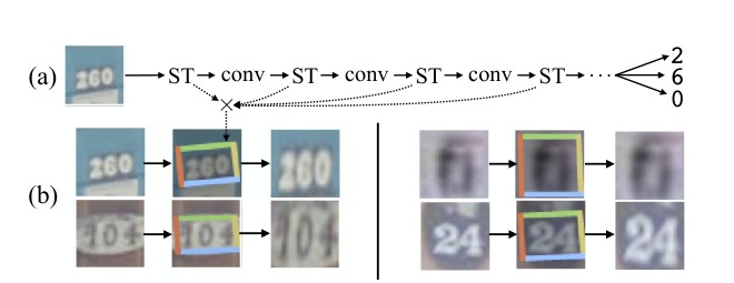
Table 2: Left: The sequence error (%) for SVHN multi-digit recognition on crops of pixels (64px), and inflated crops of (128px) which include more background. *The best reported result from [1] uses model averaging and Monte Carlo averaging, whereas the results from other models are from a single forward pass of a single model. Right: (a) The schematic of the ST-CNN Multi model. The transformations of each spatial transformer (ST) are applied to the convolutional feature map produced by the previous layer. (b) The result of the composition of the affine transformations predicted by the four spatial transformers in ST-CNN Multi, visualised on the input image.
| Model | 64px | 128px |
|---|---|---|
| Maxout CNN [10] | 4.0 | - |
| CNN (ours) | 4.0 | 5.6 |
| DRAM [1] | 3.9 | 4.5 |
| ST-CNN Single | 3.7 | 3.9 |
| ST-CNN Multi | 3.6 | 3.9 |
图为表 2 右侧的可视化。表 2:左:在 像素裁剪(64px)以及包含更多背景、放大后的 裁剪(128px)上,SVHN 多位数字识别的序列误差(%)。* [1] 报告的最好结果使用了模型平均和蒙特卡洛平均,而其他模型的结果来自单个模型的一次前向计算。右:(a) ST-CNN Multi 模型的示意。每个空间变换器(ST)的变换都施加在上一层产生的卷积特征图上。(b) 把 ST-CNN Multi 中四个空间变换器预测的仿射变换复合起来,并在输入图像上可视化的结果。
| 模型 | 64px | 128px |
|---|---|---|
| Maxout CNN [10] | 4.0 | - |
| CNN(本文) | 4.0 | 5.6 |
| DRAM [1] | 3.9 | 4.5 |
| ST-CNN Single | 3.7 | 3.9 |
| ST-CNN Multi | 3.6 | 3.9 |
background clutter (see Fig. 1 third row for an example): an FCN gets 13.2% error, a CNN gets 3.5% error, while an ST-FCN gets 2.0% error and an ST-CNN gets 1.7% error.
带有背景杂乱(例子见图 1 第三行):FCN 的误差为 13.2%,CNN 为 3.5%,而 ST-FCN 为 2.0%,ST-CNN 为 1.7%。
Looking at the results between different classes of transformation, the thin plate spline transformation (TPS) is the most powerful, being able to reduce error on elastically deformed digits by reshaping the input into a prototype instance of the digit, reducing the complexity of the task for the classification network, and does not over fit on simpler data e.g. R. Interestingly, the transformation of inputs for all ST models leads to a “standard” upright posed digit – this is the mean pose found in the training data. In Table 1 (right), we show the transformations performed for some test cases where a CNN is unable to correctly classify the digit, but a spatial transformer network can.
比较不同类别的变换可以看到,薄板样条变换(TPS)最为强大:它能把输入重塑成该数字的一个原型实例,从而降低弹性形变数字上的误差,减轻分类网络的任务复杂度,并且在更简单的数据(例如 R)上也不会过拟合。有意思的是,所有 ST 模型对输入的变换都会得到一种“标准”的端正数字——这正是训练数据中的平均姿态。表 1(右)给出了一些测试例子上所做的变换:在这些例子里 CNN 无法正确分类数字,而空间变换器网络可以。
4.2 Street View House Numbers
We now test our spatial transformer networks on a challenging real-world dataset, Street View House Numbers (SVHN) [21]. This dataset contains around 200k real world images of house numbers, with the task to recognise the sequence of numbers in each image. There are between 1 and 5 digits in each image, with a large variability in scale and spatial arrangement.
我们接下来在具有挑战性的真实世界数据集 Street View House Numbers(SVHN)[21] 上测试空间变换器网络。该数据集包含约 20 万张真实门牌号码图像,任务是识别每张图中的数字序列。每张图有 1 到 5 位数字,尺度和空间排布的变化都很大。
We follow the experimental setup as in [1, 10], where the data is preprocessed by taking crops around each digit sequence. We also use an additional more loosely cropped dataset as in [1]. We train a baseline character sequence CNN model with 11 hidden layers leading to five independent softmax classifiers, each one predicting the digit at a particular position in the sequence. This is the character sequence model used in [16], where each classifier includes a null-character output to model variable length sequences. This model matches the results obtained in [10].
我们沿用 [1, 10] 中的实验设置,预处理时在每个数字序列周围裁出 的区域。我们也如 [1] 那样,另外使用裁得更松的 数据集。我们训练一个基线字符序列 CNN 模型,它有 11 个隐层,通向五个独立的 softmax 分类器,每个分类器预测序列中某一位置的数字。这就是 [16] 中使用的字符序列模型,每个分类器都包含一个空字符输出,以便对可变长度序列建模。该模型与 [10] 中得到的结果相符。
We extend this baseline CNN to include a spatial transformer immediately following the input (ST-CNN Single), where the localisation network is a four-layer CNN. We also define another extension where before each of the first four convolutional layers of the baseline CNN, we insert a spatial transformer (ST-CNN Multi). In this case, the localisation networks are all two-layer fully connected networks with 32 units per layer. In the ST-CNN Multi model, the spatial transformer before the first convolutional layer acts on the input image as with the previous experiments, however the subsequent spatial transformers deeper in the network act on the convolutional feature maps, predicting a transformation from them and transforming these feature maps (this is visualised in Table 2 (right) (a)). This allows deeper spatial transformers to predict a transformation based on richer features rather than the raw image. All networks are trained from scratch with SGD and dropout [14], with randomly initialised weights, except for the regression layers of spatial transformers which are initialised to predict the identity transform. Affine transformations and bilinear sampling kernels are used for all spatial transformer networks in these experiments.
我们把这个基线 CNN 加以扩展,在输入之后立刻加入一个空间变换器(ST-CNN Single),其定位网络是一个四层 CNN。我们还定义了另一种扩展:在基线 CNN 的前四个卷积层之前,各插入一个空间变换器(ST-CNN Multi)。此时,定位网络都是每层 32 个单元的两层全连接网络。在 ST-CNN Multi 模型中,第一个卷积层之前的空间变换器像前面的实验一样作用在输入图像上,但网络更深处的后续空间变换器则作用在卷积特征图上,由特征图预测变换并变换这些特征图(可视化见表 2(右)(a))。这样,更深的空间变换器就可以依据更丰富的特征而不是原始图像来预测变换。所有网络都用 SGD 和 dropout [14] 从头训练,权重随机初始化,但空间变换器的回归层被初始化为预测恒等变换。这些实验中的所有空间变换器网络都使用仿射变换和双线性采样核。
The results of this experiment are shown in Table 2 (left) – the spatial transformer models obtain state-of-the-art results, reaching 3.6% error on images compared to previous state-of-the-art of 3.9% error. Interestingly on images, while other methods degrade in performance, an ST-CNN achieves 3.9% error while the previous state of the art at 4.5% error is with a recurrent attention model that uses an ensemble of models with Monte Carlo averaging – in contrast the ST-CNN models require only a single forward pass of a single model. This accuracy is achieved due to the fact that the spatial transformers crop and rescale the parts of the feature maps that correspond to the digit, focussing resolution and network capacity only on these areas (see Table 2 (right) (b)
该实验的结果见表 2(左)——空间变换器模型取得了当时最好结果,在 图像上达到 3.6% 的误差,而此前最好结果为 3.9%。有意思的是,在 图像上,其他方法的表现会下降,而 ST-CNN 达到 3.9% 的误差;此前最好结果为 4.5%,来自一个使用模型集成和蒙特卡洛平均的循环注意力模型——相比之下,ST-CNN 模型只需要对单个模型做一次前向计算。之所以能达到这一精度,是因为空间变换器裁出并重新缩放了特征图中对应数字的部分,把分辨率和网络容量都集中到这些区域(见表 2(右)(b)
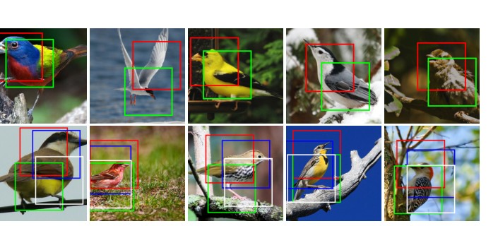
Table 3: Left: The accuracy (%) on CUB-200-2011 bird classification dataset. Spatial transformer networks with two spatial transformers (ST-CNN) and four spatial transformers (ST-CNN) in parallel outperform other models. 448px resolution images can be used with the ST-CNN without an increase in computational cost due to downsampling to 224px after the transformers. Right: The transformation predicted by the spatial transformers of ST-CNN (top row) and ST-CNN (bottom row) on the input image. Notably for the ST-CNN, one of the transformers (shown in red) learns to detect heads, while the other (shown in green) detects the body, and similarly for the ST-CNN.
| Model | Accuracy |
|---|---|
| Cimpoi ’15 [4] | 66.7 |
| Zhang ’14 [30] | 74.9 |
| Branson ’14 [2] | 75.7 |
| Lin ’15 [20] | 80.9 |
| Simon ’15 [24] | 81.0 |
| CNN (ours) 224px | 82.3 |
| ST-CNN 224px | 83.1 |
| ST-CNN 448px | 83.9 |
| ST-CNN 448px | 84.1 |
图为表 3 右侧的可视化。表 3:左:在 CUB-200-2011 鸟类分类数据集上的准确率(%)。并行使用两个空间变换器(ST-CNN)和四个空间变换器(ST-CNN)的空间变换器网络优于其他模型。ST-CNN 可以使用 448 像素分辨率的图像而不增加计算代价,因为变换器之后会降采样到 224 像素。右:ST-CNN(上行)和 ST-CNN(下行)的空间变换器在输入图像上预测的变换。值得注意的是,对 ST-CNN 而言,其中一个变换器(红色)学会了检测头部,另一个(绿色)检测身体;ST-CNN 也有类似情况。
| 模型 | 准确率 |
|---|---|
| Cimpoi ’15 [4] | 66.7 |
| Zhang ’14 [30] | 74.9 |
| Branson ’14 [2] | 75.7 |
| Lin ’15 [20] | 80.9 |
| Simon ’15 [24] | 81.0 |
| CNN(本文) 224px | 82.3 |
| ST-CNN 224px | 83.1 |
| ST-CNN 448px | 83.9 |
| ST-CNN 448px | 84.1 |
for some examples). In terms of computation speed, the ST-CNN Multi model is only 6% slower (forward and backward pass) than the CNN.
给出了一些例子)。就计算速度而言,ST-CNN Multi 模型(前向和反向)只比 CNN 慢 6%。
4.3 Fine-Grained Classification
In this section, we use a spatial transformer network with multiple transformers in parallel to perform fine-grained bird classification. We evaluate our models on the CUB-200-2011 birds dataset [28], containing 6k training images and 5.8k test images, covering 200 species of birds. The birds appear at a range of scales and orientations, are not tightly cropped, and require detailed texture and shape analysis to distinguish. In our experiments, we only use image class labels for training.
本节使用带有多个并行变换器的空间变换器网络,做细粒度鸟类分类。我们在 CUB-200-2011 鸟类数据集 [28] 上评估模型,该数据集包含 6 千张训练图像和 5.8 千张测试图像,覆盖 200 种鸟。这些鸟出现在多种尺度和朝向上,并没有被紧致裁剪,要区分它们需要对纹理和形状做细致分析。在我们的实验中,训练只使用图像类别标签。
We consider a strong baseline CNN model – an Inception architecture with batch normalisation [15] pre-trained on ImageNet [22] and fine-tuned on CUB – which by itself achieves state-of-the-art accuracy of 82.3% (previous best result is 81.0% [24]). We then train a spatial transformer network, ST-CNN, which contains 2 or 4 parallel spatial transformers, parameterised for attention and acting on the input image. Discriminative image parts, captured by the transformers, are passed to the part description sub-nets (each of which is also initialised by Inception). The resulting part representations are concatenated and classified with a single softmax layer. The whole architecture is trained on image class labels end-to-end with backpropagation (details in supplementary material).
我们采用一个较强的基线 CNN 模型——带有批归一化 [15]、在 ImageNet [22] 上预训练并在 CUB 上微调的 Inception 结构——它本身就达到了当时最好的 82.3% 准确率(此前最好结果为 81.0% [24])。随后我们训练空间变换器网络 ST-CNN,其中包含 2 个或 4 个并行的空间变换器,按注意力方式参数化,并作用在输入图像上。变换器捕捉到的有判别力的图像部件,被送入部件描述子网络(每个子网络同样由 Inception 初始化)。得到的部件表示被拼接起来,再用单个 softmax 层分类。整个结构只用图像类别标签、以反向传播做端到端训练(细节见补充材料)。
The results are shown in Table 3 (left). The ST-CNN achieves an accuracy of 84.1%, outperforming the baseline by 1.8%. In the visualisations of the transforms predicted by ST-CNN (Table 3 (right)) one can see interesting behaviour has been learnt: one spatial transformer (red) has learnt to become a head detector, while the other (green) fixates on the central part of the body of a bird. The resulting output from the spatial transformers for the classification network is a somewhat pose-normalised representation of a bird. While previous work such as [2] explicitly define parts of the bird, training separate detectors for these parts with supplied keypoint training data, the ST-CNN is able to discover and learn part detectors in a data-driven manner without any additional supervision. In addition, spatial transformers allows for the use of 448px resolution input images without any impact on performance, as the output of the transformed 448px images are sampled at 224px before being processed.
结果见表 3(左)。ST-CNN 达到 84.1% 的准确率,比基线高 1.8%。在 ST-CNN 所预测变换的可视化中(表 3(右)),可以看到已经学到了有意思的行为:一个空间变换器(红色)学会了成为头部检测器,另一个(绿色)则盯住鸟身体的中央部分。空间变换器送给分类网络的输出,因而是一种在一定程度上姿态归一化的鸟类表示。以往如 [2] 等工作会显式定义鸟的各个部件,并用提供的关键点训练数据为这些部件分别训练检测器;而 ST-CNN 能够以数据驱动的方式发现并学习部件检测器,无需任何额外监督。此外,空间变换器还允许使用 448 像素分辨率的输入图像而不影响性能,因为变换后的 448 像素图像会在处理前被采样到 224 像素。
5 Conclusion
In this paper we introduced a new self-contained module for neural networks – the spatial transformer. This module can be dropped into a network and perform explicit spatial transformations of features, opening up new ways for neural networks to model data, and is learnt in an end-to-end fashion, without making any changes to the loss function. While CNNs provide an incredibly strong baseline, we see gains in accuracy using spatial transformers across multiple tasks, resulting in state-of-the-art performance. Furthermore, the regressed transformation parameters from the spatial transformer are available as an output and could be used for subsequent tasks. While we only explore feed-forward networks in this work, early experiments show spatial transformers to be powerful in recurrent models, and useful for tasks requiring the disentangling of object reference frames.
本文为神经网络引入了一种新的自包含模块——空间变换器。这个模块可以插入网络,对特征做显式的空间变换,为神经网络建模数据开辟了新的途径,并且以端到端的方式学习,不必改动损失函数。尽管 CNN 已经是非常强的基线,我们在多个任务上仍看到使用空间变换器带来的准确率提升,并达到当时最好成绩。此外,空间变换器回归出的变换参数可以作为输出,供后续任务使用。虽然本文只考察了前馈网络,但初步实验表明,空间变换器在循环模型中也很有效,并且有助于需要把物体参考系分离出来的任务。
References
[1] J. Ba, V. Mnih, and K. Kavukcuoglu. Multiple object recognition with visual attention. ICLR, 2015.
[2] S. Branson, G. Van Horn, S. Belongie, and P. Perona. Bird species categorization using pose normalized deep convolutional nets. BMVC., 2014.
[3] J. Bruna and S. Mallat. Invariant scattering convolution networks. IEEE PAMI, 35(8):1872–1886, 2013.
[4] M. Cimpoi, S. Maji, and A. Vedaldi. Deep filter banks for texture recognition and segmentation. In CVPR, 2015.
[5] T. S. Cohen and M. Welling. Transformation properties of learned visual representations. ICLR, 2015.
[6] D. Erhan, C. Szegedy, A. Toshev, and D. Anguelov. Scalable object detection using deep neural networks. In CVPR, 2014.
[7] B. J. Frey and N. Jojic. Fast, large-scale transformation-invariant clustering. In NIPS, 2001.
[8] R. Gens and P. M. Domingos. Deep symmetry networks. In NIPS, 2014.
[9] R. B. Girshick, J. Donahue, T. Darrell, and J. Malik. Rich feature hierarchies for accurate object detection and semantic segmentation. In CVPR, 2014.
[10] I. J. Goodfellow, Y. Bulatov, J. Ibarz, S. Arnoud, and V. Shet. Multi-digit number recognition from street view imagery using deep convolutional neural networks. arXiv:1312.6082, 2013.
[11] K. Gregor, I. Danihelka, A. Graves, and D. Wierstra. Draw: A recurrent neural network for image generation. ICML, 2015.
[12] G. E. Hinton. A parallel computation that assigns canonical object-based frames of reference. In IJCAI, 1981.
[13] G. E. Hinton, A. Krizhevsky, and S. D. Wang. Transforming auto-encoders. In ICANN. 2011.
[14] G. E. Hinton, N. Srivastava, A. Krizhevsky, I. Sutskever, and R. Salakhutdinov. Improving neural networks by preventing co-adaptation of feature detectors. CoRR, abs/1207.0580, 2012.
[15] S. Ioffe and C. Szegedy. Batch normalization: Accelerating deep network training by reducing internal covariate shift. ICML, 2015.
[16] M. Jaderberg, K. Simonyan, A. Vedaldi, and A. Zisserman. Synthetic data and artificial neural networks for natural scene text recognition. NIPS DLW, 2014.
[17] A. Kanazawa, A. Sharma, and D. Jacobs. Locally scale-invariant convolutional neural networks. In NIPS, 2014.
[18] Y. LeCun, L. Bottou, Y. Bengio, and P. Haffner. Gradient-based learning applied to document recognition. Proceedings of the IEEE, 86(11):2278–2324, 1998.
[19] K. Lenc and A. Vedaldi. Understanding image representations by measuring their equivariance and equivalence. CVPR, 2015.
[20] T. Lin, A. RoyChowdhury, and S. Maji. Bilinear CNN models for fine-grained visual recognition. arXiv:1504.07889, 2015.
[21] Y. Netzer, T. Wang, A. Coates, A. Bissacco, B. Wu, and A. Y. Ng. Reading digits in natural images with unsupervised feature learning. In NIPS DLW, 2011.
[22] O. Russakovsky, J. Deng, H. Su, J. Krause, S. Satheesh, S. Ma, Z. Huang, A. Karpathy, A. Khosla, M. Bernstein, et al. Imagenet large scale visual recognition challenge. arXiv:1409.0575, 2014.
[23] P. Sermanet, A. Frome, and E. Real. Attention for fine-grained categorization. arXiv:1412.7054, 2014.
[24] M. Simon and E. Rodner. Neural activation constellations: Unsupervised part model discovery with convolutional networks. arXiv:1504.08289, 2015.
[25] K. Sohn and H. Lee. Learning invariant representations with local transformations. arXiv:1206.6418, 2012.
[26] M. F. Stollenga, J. Masci, F. Gomez, and J. Schmidhuber. Deep networks with internal selective attention through feedback connections. In NIPS, 2014.
[27] T. Tieleman. Optimizing Neural Networks that Generate Images. PhD thesis, University of Toronto, 2014.
[28] C. Wah, S. Branson, P. Welinder, P. Perona, and S. Belongie. The Caltech-UCSD Birds-200-2011 dataset. 2011.
[29] K. Xu, J. Ba, R. Kiros, K. Cho, A. Courville, R. Salakhutdinov, R. Zemel, and Y. Bengio. Show, attend and tell: Neural image caption generation with visual attention. ICML, 2015.
[30] X. Zhang, J. Zou, X. Ming, K. He, and J. Sun. Efficient and accurate approximations of nonlinear convolutional networks. arXiv:1411.4229, 2014.