Outrageously Large Neural Networks: The Sparsely-Gated Mixture-of-Experts Layer

大得离谱的神经网络：稀疏门控混合专家层

Noam Shazeer Affiliation:  Google Brain, {noam,azalia,andydavis,qvl,geoffhinton,jeff}@google.com    Azalia Mirhoseini † † thanks: Equally major contributors † † thanks: Work done as a member of the Google Brain Residency program (g.co/brainresidency) Affiliation:  Google Brain, {noam,azalia,andydavis,qvl,geoffhinton,jeff}@google.com    Krzysztof Maziarz ∗ Affiliation:  Jagiellonian University, Cracow, krzysztof.maziarz@student.uj.edu.pl    Andy Davis Affiliation:  Google Brain, {noam,azalia,andydavis,qvl,geoffhinton,jeff}@google.com    Quoc Le Affiliation:  Google Brain, {noam,azalia,andydavis,qvl,geoffhinton,jeff}@google.com    Geoffrey Hinton Affiliation:  Google Brain, {noam,azalia,andydavis,qvl,geoffhinton,jeff}@google.com    Jeff Dean Affiliation:  Google Brain, {noam,azalia,andydavis,qvl,geoffhinton,jeff}@google.com

Abstract

摘要

The capacity of a neural network to absorb information is limited by its number of parameters. Conditional computation, where parts of the network are active on a per-example basis, has been proposed in theory as a way of dramatically increasing model capacity without a proportional increase in computation. In practice, however, there are significant algorithmic and performance challenges. In this work, we address these challenges and finally realize the promise of conditional computation, achieving greater than 1000x improvements in model capacity with only minor losses in computational efficiency on modern GPU clusters. We introduce a Sparsely-Gated Mixture-of-Experts layer (MoE), consisting of up to thousands of feed-forward sub-networks. A trainable gating network determines a sparse combination of these experts to use for each example. We apply the MoE to the tasks of language modeling and machine translation, where model capacity is critical for absorbing the vast quantities of knowledge available in the training corpora. We present model architectures in which a MoE with up to 137 billion parameters is applied convolutionally between stacked LSTM layers. On large language modeling and machine translation benchmarks, these models achieve significantly better results than state-of-the-art at lower computational cost.

神经网络吸收信息的容量受参数量限制。有人在理论上提出条件计算：网络的不同部分按每个样本分别激活，从而在计算量不成比例增加的情况下大幅提高模型容量。实践中却有显著的算法与性能挑战。本文应对这些挑战，并终于兑现条件计算的承诺：在现代 GPU 集群上，模型容量提高超过 1000 倍，计算效率只受很小损失。我们引入稀疏门控混合专家层（MoE），由多达数千个前馈子网络组成。可训练的门控网络为每个样本决定使用这些专家的一个稀疏组合。我们把 MoE 用到语言模型与机器翻译上，这些任务需要很大容量来吸收训练语料中的大量知识。我们给出的结构把最多 1370 亿参数的 MoE 卷积式地插在堆叠的 LSTM 层之间。在大型语言建模与机器翻译基准上，这些模型以更低的计算代价显著超过当时最优结果。

1 Introduction and Related Work

1 引言与相关工作

1.1 Conditional Computation

1.1 条件计算

Exploiting scale in both training data and model size has been central to the success of deep learning. When datasets are sufficiently large, increasing the capacity (number of parameters) of neural networks can give much better prediction accuracy. This has been shown in domains such as text (Sutskever et al., 2014; Bahdanau et al., 2014; Jozefowicz et al., 2016; Wu et al., 2016), images (Krizhevsky et al., 2012; Le et al., 2012), and audio (Hinton et al., 2012; Amodei et al., 2015). For typical deep learning models, where the entire model is activated for every example, this leads to a roughly quadratic blow-up in training costs, as both the model size and the number of training examples increase. Unfortunately, the advances in computing power and distributed computation fall short of meeting such demand.

同时扩大训练数据与模型规模，是深度学习成功的核心。当数据集足够大时，增加神经网络的容量（参数量）能带来好得多的预测精度。这一点已在文本（Sutskever 等，2014；Bahdanau 等，2014；Jozefowicz 等，2016；Wu 等，2016）、图像（Krizhevsky 等，2012；Le 等，2012）与音频（Hinton 等，2012；Amodei 等，2015）等领域得到验证。对典型深度学习模型而言，每个样本都会激活整个模型，于是当模型规模与训练样本数同时增加时，训练代价大致呈二次膨胀。遗憾的是，算力与分布式计算的进步还赶不上这种需求。

Various forms of conditional computation have been proposed as a way to increase model capacity without a proportional increase in computational costs (Davis & Arel, 2013; Bengio et al., 2013; Eigen et al., 2013; Ludovic Denoyer, 2014; Cho & Bengio, 2014; Bengio et al., 2015; Almahairi et al., 2015). In these schemes, large parts of a network are active or inactive on a per-example basis. The gating decisions may be binary or sparse and continuous, stochastic or deterministic. Various forms of reinforcement learning and back-propagation are proposed for trarining the gating decisions.

人们提出过多种条件计算，希望在计算代价不成比例增加的情况下提高模型容量（Davis 与 Arel，2013；Bengio 等，2013；Eigen 等，2013；Ludovic Denoyer，2014；Cho 与 Bengio，2014；Bengio 等，2015；Almahairi 等，2015）。这些方案里，网络的很大部分会按每个样本分别处于激活或关闭状态。门控决策可以是二元或稀疏连续的，也可以是随机或确定性的。训练门控决策则提出过各种强化学习与反向传播形式。

While these ideas are promising in theory, no work to date has yet demonstrated massive improvements in model capacity, training time, or model quality. We blame this on a combination of the following challenges:

这些想法理论上很有希望，但迄今还没有工作展示出模型容量、训练时间或模型质量上的大幅改进。我们认为原因是以下挑战的叠加：

• • Modern computing devices, especially GPUs, are much faster at arithmetic than at branching. Most of the works above recognize this and propose turning on/off large chunks of the network with each gating decision.

• • 现代计算设备、尤其是 GPU，做算术远快于做分支。上述工作大多认识到这一点，并提议每次门控决策打开或关闭网络的很大一块。

• • Large batch sizes are critical for performance, as they amortize the costs of parameter transfers and updates. Conditional computation reduces the batch sizes for the conditionally active chunks of the network.

• • 大批次对性能至关重要，因为它可以摊销参数传输与更新的代价。条件计算会减小网络中按条件激活的那些块的批次大小。

• • Network bandwidth can be a bottleneck. A cluster of GPUs may have computational power thousands of times greater than the aggregate inter-device network bandwidth. To be computationally efficient, the relative computational versus network demands of an algorithm must exceed this ratio. Embedding layers, which can be seen as a form of conditional computation, are handicapped by this very problem. Since the embeddings generally need to be sent across the network, the number of (example, parameter) interactions is limited by network bandwidth instead of computational capacity.

• • 网络带宽可能成为瓶颈。一个 GPU 集群的计算能力可能比设备间总带宽高出数千倍。要想计算高效，算法的相对计算需求与网络需求之比必须超过这一比值。嵌入层可以看成一种条件计算，恰恰受这个问题拖累。由于嵌入通常需要跨网络传送，（样本，参数）交互次数受网络带宽而不是计算能力限制。

• • Depending on the scheme, loss terms may be necessary to achieve the desired level of sparsity per-chunk and/or per example. Bengio et al. (2015) use three such terms. These issues can affect both model quality and load-balancing.

• • 视具体方案而定，可能需要额外的损失项，才能达到每块和/或每个样本所希望的稀疏度。Bengio 等（2015）用了三项这样的损失。这些问题既影响模型质量，也影响负载均衡。

• • Model capacity is most critical for very large data sets. The existing literature on conditional computation deals with relatively small image recognition data sets consisting of up to 600,000 images. It is hard to imagine that the labels of these images provide a sufficient signal to adequately train a model with millions, let alone billions of parameters.

• • 模型容量对非常大的数据集最为关键。现有条件计算文献处理的是相对较小的图像识别数据集，最多约 60 万张图。很难想象这些图像的标签能提供足够信号，去充分训练一个百万、更不用说十亿参数的模型。

In this work, we for the first time address all of the above challenges and finally realize the promise of conditional computation. We obtain greater than 1000x improvements in model capacity with only minor losses in computational efficiency and significantly advance the state-of-the-art results on public language modeling and translation data sets.

本文首次同时应对上述全部挑战，并终于兑现条件计算的承诺。我们在计算效率只受很小损失的情况下，把模型容量提高超过 1000 倍，并在公开的语言建模与翻译数据集上显著推进了当时最优结果。

1.2 Our Approach: The Sparsely-Gated Mixture-of-Experts Layer

1.2 我们的方法：稀疏门控混合专家层

Our approach to conditional computation is to introduce a new type of general purpose neural network component: a Sparsely-Gated Mixture-of-Experts Layer (MoE). The MoE consists of a number of experts, each a simple feed-forward neural network, and a trainable gating network which selects a sparse combination of the experts to process each input (see Figure 1). All parts of the network are trained jointly by back-propagation.

我们对条件计算的做法，是引入一类新的通用神经网络组件：稀疏门控混合专家层（MoE）。MoE 由若干专家组成，每个专家是一个简单的前馈神经网络，再加上一个可训练的门控网络，为每个输入选择专家的一个稀疏组合（见图 1）。网络的所有部分通过反向传播联合训练。

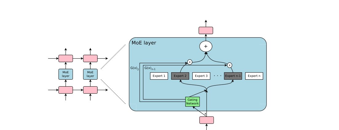
Figure 1: A Mixture of Experts (MoE) layer embedded within a recurrent language model. In this case, the sparse gating function selects two experts to perform computations. Their outputs are modulated by the outputs of the gating network.

图 1：嵌入在循环语言模型中的混合专家（MoE）层。本例中，稀疏门控函数选出两个专家进行计算。它们的输出再由门控网络的输出加以调制。

While the introduced technique is generic, in this paper we focus on language modeling and machine translation tasks, which are known to benefit from very large models. In particular, we apply a MoE convolutionally between stacked LSTM layers (Hochreiter & Schmidhuber, 1997), as in Figure 1. The MoE is called once for each position in the text, selecting a potentially different combination of experts at each position. The different experts tend to become highly specialized based on syntax and semantics (see Appendix E Table 9). On both language modeling and machine translation benchmarks, we improve on best published results at a fraction of the computational cost.

所引入的技术是通用的，但本文聚焦语言模型与机器翻译，这两类任务已知能从很大的模型中受益。具体来说，我们如图 1 所示，把 MoE 卷积式地插在堆叠的 LSTM 层（Hochreiter 与 Schmidhuber，1997）之间。文本中每个位置都会调用一次 MoE，从而在每个位置选择可能不同的专家组合。不同专家往往会按句法与语义高度特化（见附录 E 表 9）。在语言建模与机器翻译基准上，我们都以一小部分计算代价改进了此前已发表的最好结果。

1.3 Related work on Mixtures of Experts

1.3 混合专家的相关工作

Since its introduction more than two decades ago (Jacobs et al., 1991; Jordan & Jacobs, 1994), the mixture-of-experts approach has been the subject of much research. Different types of expert architectures hae been proposed such as SVMs (Collobert et al., 2002), Gaussian Processes (Tresp, 2001; Theis & Bethge, 2015; Deisenroth & Ng, 2015), Dirichlet Processes (Shahbaba & Neal, 2009), and deep networks. Other work has focused on different expert configurations such as a hierarchical structure (Yao et al., 2009), infinite numbers of experts (Rasmussen & Ghahramani, 2002), and adding experts sequentially (Aljundi et al., 2016). Garmash & Monz (2016) suggest an ensemble model in the format of mixture of experts for machine translation. The gating network is trained on a pre-trained ensemble NMT model.

自二十多年前提出以来（Jacobs 等，1991；Jordan 与 Jacobs，1994），混合专家方法已有大量研究。人们提出过不同类型的专家结构，例如 SVM（Collobert 等，2002）、高斯过程（Tresp，2001；Theis 与 Bethge，2015；Deisenroth 与 Ng，2015）、Dirichlet 过程（Shahbaba 与 Neal，2009）以及深度网络。另一些工作关注不同的专家配置，例如层次结构（Yao 等，2009）、无穷多个专家（Rasmussen 与 Ghahramani，2002），以及依次增加专家（Aljundi 等，2016）。Garmash 与 Monz（2016）为机器翻译提出一种混合专家形式的集成模型。门控网络在已预训练的集成 NMT 模型上训练。

The works above concern top-level mixtures of experts. The mixture of experts is the whole model. Eigen et al. (2013) introduce the idea of using multiple MoEs with their own gating networks as parts of a deep model. It is intuitive that the latter approach is more powerful, since complex problems may contain many sub-problems each requiring different experts. They also allude in their conclusion to the potential to introduce sparsity, turning MoEs into a vehicle for computational computation.

上述工作关心的是顶层混合专家：混合专家就是整个模型。Eigen 等（2013）提出把多个各有门控网络的 MoE 作为深度模型的组成部分。后一种做法直觉上更强，因为复杂问题可能包含许多子问题，每个都需要不同的专家。他们在结论中也提到引入稀疏性的可能，从而把 MoE 变成条件计算的载体。

Our work builds on this use of MoEs as a general purpose neural network component. While Eigen et al. (2013) uses two stacked MoEs allowing for two sets of gating decisions, our convolutional application of the MoE allows for different gating decisions at each position in the text. We also realize sparse gating and demonstrate its use as a practical way to massively increase model capacity.

我们的工作建立在把 MoE 当作通用神经网络组件这一用法之上。Eigen 等（2013）使用两个堆叠的 MoE，允许两套门控决策；我们把 MoE 卷积式地应用，从而允许文本每个位置有不同的门控决策。我们还实现了稀疏门控，并展示它作为大规模提高模型容量的实用途径。

2 The Structure of the Mixture-of-Experts layer

2 混合专家层的结构

The Mixture-of-Experts (MoE) layer consists of a set of $n$ “expert networks" $E_{1},\cdots,E_{n}$, and a “gating network" $G$ whose output is a sparse $n$-dimensional vector. Figure 1 shows an overview of the MoE module. The experts are themselves neural networks, each with their own parameters. Although in principle we only require that the experts accept the same sized inputs and produce the same-sized outputs, in our initial investigations in this paper, we restrict ourselves to the case where the models are feed-forward networks with identical architectures, but with separate parameters.

混合专家（MoE）层由一组 $n$ 个“专家网络” $E_{1},\cdots,E_{n}$ 以及一个输出为稀疏 $n$ 维向量的“门控网络” $G$ 组成。图 1 给出 MoE 模块概览。专家本身也是神经网络，各自有自己的参数。原则上我们只要求专家接受相同尺寸的输入并产生相同尺寸的输出；本文的初步研究中，我们把自己限制在各专家是结构相同、参数分开的前馈网络这一情形。

Let us denote by $G(x)$ and $E_{i}(x)$ the output of the gating network and the output of the $i$-th expert network for a given input $x$. The output $y$ of the MoE module can be written as follows:

令 $G(x)$ 与 $E_{i}(x)$ 分别表示门控网络的输出以及第 $i$ 个专家网络对给定输入 $x$ 的输出。MoE 模块的输出 $y$ 可以写成：

$$y=\sum_{i=1}^{n}G(x)_{i}E_{i}(x) \tag{1}$$

We save computation based on the sparsity of the output of $G(x)$. Wherever $G(x)_{i}=0$, we need not compute $E_{i}(x)$. In our experiments, we have up to thousands of experts, but only need to evaluate a handful of them for every example. If the number of experts is very large, we can reduce the branching factor by using a two-level hierarchical MoE. In a hierarchical MoE, a primary gating network chooses a sparse weighted combination of “experts", each of which is itself a secondary mixture-of-experts with its own gating network. In the following we focus on ordinary MoEs. We provide more details on hierarchical MoEs in Appendix B.

我们利用 $G(x)$ 输出的稀疏性来节省计算。凡是 $G(x)_{i}=0$ 的地方，就不必计算 $E_{i}(x)$。实验中我们最多有数千个专家，但每个样本只需评估其中少数几个。若专家数非常大，可以用两层层次化 MoE 来降低分支因子。在层次化 MoE 中，主门控网络选择“专家”的一个稀疏加权组合，而每个“专家”本身又是带自己门控网络的次级混合专家。下文聚焦普通 MoE。层次化 MoE 的更多细节见附录 B。

Our implementation is related to other models of conditional computation. A MoE whose experts are simple weight matrices is similar to the parameterized weight matrix proposed in (Cho & Bengio, 2014). A MoE whose experts have one hidden layer is similar to the block-wise dropout described in (Bengio et al., 2015), where the dropped-out layer is sandwiched between fully-activated layers.

我们的实现与其他条件计算模型有关。专家是简单权重矩阵的 MoE，类似于 Cho 与 Bengio（2014）提出的参数化权重矩阵。专家带一个隐藏层的 MoE，类似于 Bengio 等（2015）描述的分块 dropout，其中被丢弃的层夹在完全激活的层之间。

2.1 Gating Network

2.1 门控网络

Softmax Gating:

A simple choice of non-sparse gating function (Jordan & Jacobs, 1994) is to multiply the input by a trainable weight matrix $W_{g}$ and then apply the $Softmax$ function.

Softmax 门控：

一种简单的非稀疏门控函数（Jordan 与 Jacobs，1994）是把输入乘以可训练权重矩阵 $W_{g}$，再施加 $Softmax$ 函数。

$$G_{\sigma}(x)=Softmax(x\cdot W_{g}) \tag{2}$$

Noisy Top-K Gating:

We add two components to the Softmax gating network: sparsity and noise. Before taking the softmax function, we add tunable Gaussian noise, then keep only the top k values, setting the rest to $-\infty$ (which causes the corresponding gate values to equal $0$). The sparsity serves to save computation, as described above. While this form of sparsity creates some theoretically scary discontinuities in the output of gating function, we have not yet observed this to be a problem in practice. The noise term helps with load balancing, as will be discussed in Appendix A. The amount of noise per component is controlled by a second trainable weight matrix $W_{noise}$.

带噪声的 Top-K 门控：

我们在 Softmax 门控网络上加了两个成分：稀疏性与噪声。在取 softmax 之前，我们加入可调的高斯噪声，然后只保留前 k 个值，其余设为 $-\infty$（这会使相应门控值等于 $0$）。稀疏性用来节省计算，如上所述。这种稀疏性会在门控函数输出中造成一些理论上令人不安的不连续，但我们实践中尚未观察到这成为问题。噪声项有助于负载均衡，将在附录 A 讨论。每个分量的噪声量由第二个可训练权重矩阵 $W_{noise}$ 控制。

$$G(x)=Softmax(KeepTopK(H(x),k)) \tag{3}$$

$$H(x)_{i}=(x\cdot W_{g})_{i}+StandardNormal()\cdot Softplus((x\cdot W_{noise})_{i}) \tag{4}$$

$KeepTopK(v,k)_{i}=\begin{cases}v_{i}&\text{ifv_{i}$is in the top$k$elements of$v$.}\
-\infty&\text{otherwise.}\end{cases} \tag{5}$$

$$KeepTopK(v,k)_{i}=\begin{cases}v_{i}&\text{if $v_{i}$ is in the top $k$ elements of $v$.}\\-\infty&\text{otherwise.}\end{cases} \tag{5}$$

Training the Gating Network

We train the gating network by simple back-propagation, along with the rest of the model. If we choose $k>1$, the gate values for the top k experts have nonzero derivatives with respect to the weights of the gating network. This type of occasionally-sensitive behavior is described in (Bengio et al., 2013) with respect to noisy rectifiers. Gradients also back-propagate through the gating network to its inputs. Our method differs here from (Bengio et al., 2015) who use boolean gates and a REINFORCE-style approach to train the gating network.

训练门控网络

我们用简单的反向传播，与模型其余部分一起训练门控网络。若选择 $k>1$，前 k 个专家的门控值相对于门控网络权重具有非零导数。这种偶尔敏感的行为，Bengio 等（2013）曾就带噪声的整流器描述过。梯度也会通过门控网络回传到其输入。我们的方法在此不同于 Bengio 等（2015）：他们使用布尔门，并用类似 REINFORCE 的方式训练门控网络。

3 Addressing Performance Challenges

3 应对性能挑战

3.1 The Shrinking Batch Problem

3.1 批次缩小问题

On modern CPUs and GPUs, large batch sizes are necessary for computational efficiency, so as to amortize the overhead of parameter loads and updates. If the gating network chooses $k$ out of $n$ experts for each example, then for a batch of $b$ examples, each expert receives a much smaller batch of approximately $\frac{kb}{n}\ll b$ examples. This causes a naive MoE implementation to become very inefficient as the number of experts increases. The solution to this shrinking batch problem is to make the original batch size as large as possible. However, batch size tends to be limited by the memory necessary to store activations between the forwards and backwards passes. We propose the following techniques for increasing the batch size:

在现代 CPU 与 GPU 上，大批次对计算效率是必要的，以便摊销加载与更新参数的开销。若门控网络对每个样本从 $n$ 个专家中选出 $k$ 个，那么对大小为 $b$ 的批次，每个专家大约只收到 $\frac{kb}{n}\ll b$ 个样本。专家数增加时，朴素的 MoE 实现会因此变得非常低效。解决批次缩小问题的办法是让原始批次尽可能大。但批次大小往往受前向与反向之间存储激活所需内存的限制。我们提出以下增大批次的技术：

Mixing Data Parallelism and Model Parallelism:

In a conventional distributed training setting, multiple copies of the model on different devices asynchronously process distinct batches of data, and parameters are synchronized through a set of parameter servers. In our technique, these different batches run synchronously so that they can be combined for the MoE layer. We distribute the standard layers of the model and the gating network according to conventional data-parallel schemes, but keep only one shared copy of each expert. Each expert in the MoE layer receives a combined batch consisting of the relevant examples from all of the data-parallel input batches. The same set of devices function as data-parallel replicas (for the standard layers and the gating networks) and as model-parallel shards (each hosting a subset of the experts). If the model is distributed over $d$ devices, and each device processes a batch of size $b$, each expert receives a batch of approximately $\frac{kbd}{n}$ examples. Thus, we achieve a factor of $d$ improvement in expert batch size.

混合数据并行与模型并行：

在常规分布式训练中，不同设备上的多份模型副本异步处理不同数据批次，参数通过一组参数服务器同步。我们的做法是让这些不同批次同步运行，以便在 MoE 层合并。标准层与门控网络按常规数据并行方案分布，但每个专家只保留一份共享副本。MoE 层中的每个专家收到一个合并批次，由所有数据并行输入批次中的相关样本组成。同一组设备既作为数据并行副本（对标准层与门控网络），又作为模型并行分片（各自托管一部分专家）。若模型分布在 $d$ 台设备上，每台处理大小为 $b$ 的批次，每个专家大约收到 $\frac{kbd}{n}$ 个样本。于是专家批次大小提高了 $d$ 倍。

In the case of a hierarchical MoE (Section B), the primary gating network employs data parallelism, and the secondary MoEs employ model parallelism. Each secondary MoE resides on one device.

对层次化 MoE（附录 B），主门控网络采用数据并行，次级 MoE 采用模型并行。每个次级 MoE 驻留在一台设备上。

This technique allows us to increase the number of experts (and hence the number of parameters) by proportionally increasing the number of devices in the training cluster. The total batch size increases, keeping the batch size per expert constant. The memory and bandwidth requirements per device also remain constant, as do the step times, as does the amount of time necessary to process a number of training examples equal to the number of parameters in the model. It is our goal to train a trillion-parameter model on a trillion-word corpus. We have not scaled our systems this far as of the writing of this paper, but it should be possible by adding more hardware.

这一技术使我们能通过按比例增加训练集群中的设备数，来增加专家数（从而增加参数量）。总批次增大，每个专家的批次保持不变。每台设备的内存与带宽需求、步进时间，以及处理与模型参数量相当的训练样本所需时间也都保持不变。我们的目标是在一万亿词的语料上训练一万亿参数的模型。写本文时我们尚未扩展到这一规模，但通过增加硬件应当可以做到。

Taking Advantage of Convolutionality:

In our language models, we apply the same MoE to each time step of the previous layer. If we wait for the previous layer to finish, we can apply the MoE to all the time steps together as one big batch. Doing so increases the size of the input batch to the MoE layer by a factor of the number of unrolled time steps.

利用卷积性：

在我们的语言模型中，我们对上一层的每个时间步应用同一个 MoE。若等到上一层完成，就可以把 MoE 一次性应用到所有时间步，当作一个大批次。这会把 MoE 层的输入批次按展开时间步数放大。

Increasing Batch Size for a Recurrent MoE:

We suspect that even more powerful models may involve applying a MoE recurrently. For example, the weight matrices of a LSTM or other RNN could be replaced by a MoE. Sadly, such models break the convolutional trick from the last paragraph, since the input to the MoE at one timestep depends on the output of the MoE at the previous timestep. Gruslys et al. (2016) describe a technique for drastically reducing the number of stored activations in an unrolled RNN, at the cost of recomputing forward activations. This would allow for a large increase in batch size.

增大循环 MoE 的批次：

我们猜想，更强的模型可能涉及循环地应用 MoE。例如，LSTM 或其他 RNN 的权重矩阵可以由 MoE 替换。可惜这样的模型会打破上一段的卷积技巧，因为某一时间步 MoE 的输入依赖于上一时间步 MoE 的输出。Gruslys 等（2016）描述了一种大幅减少展开 RNN 中所存激活数量的技术，代价是重新计算前向激活。这会允许批次大幅增加。

3.2 Network Bandwidth

3.2 网络带宽

Another major performance concern in distributed computing is network bandwidth. Since the experts are stationary (see above) and the number of gating parameters is small, most of the communication involves sending the inputs and outputs of the experts across the network. To maintain computational efficiency, the ratio of an expert’s computation to the size of its input and output must exceed the ratio of computational to network capacity of the computing device. For GPUs, this may be thousands to one. In our experiments, we use experts with one hidden layer containing thousands of RELU-activated units. Since the weight matrices in the expert have sizes $input$${size}\times hidden$${size}$ and $hidden$${size}\times output$${size}$, the ratio of computation to input and output is equal to the size of the hidden layer. Conveniently, we can increase computational efficiency simply by using a larger hidden layer, or more hidden layers.

分布式计算中另一个主要性能问题是网络带宽。由于专家是固定的（见上）且门控参数很少，大部分通信是把专家的输入与输出送过网络。要保持计算效率，专家的计算量与其输入输出大小之比，必须超过计算设备的计算能力与网络能力之比。对 GPU，这可能是数千比一。实验中我们使用带一个隐藏层、含数千个 ReLU 激活单元的专家。由于专家中权重矩阵的尺寸为 $input\_size\times hidden\_size$ 与 $hidden\_size\times output\_size$，计算量与输入输出之比等于隐藏层大小。方便的是，只需使用更大的隐藏层或更多隐藏层，就可以提高计算效率。

4 Balancing Expert Utilization

4 平衡专家利用率

We have observed that the gating network tends to converge to a state where it always produces large weights for the same few experts. This imbalance is self-reinforcing, as the favored experts are trained more rapidly and thus are selected even more by the gating network. Eigen et al. (2013) describe the same phenomenon, and use a hard constraint at the beginning of training to avoid this local minimum. Bengio et al. (2015) include a soft constraint on the batch-wise average of each gate.[^1]

我们观察到，门控网络往往会收敛到总是给少数几个相同专家产生大权重的状态。这种不均衡会自我强化：受青睐的专家训练得更快，因而更常被门控网络选中。Eigen 等（2013）描述了同一现象，并在训练开始时使用硬约束来避开这一局部极小。Bengio 等（2015）对每个门在批次上的平均值加入软约束。[^1]

We take a soft constraint approach. We define the importance of an expert relative to a batch of training examples to be the batchwise sum of the gate values for that expert. We define an additional loss $L_{importance}$, which is added to the overall loss function for the model. This loss is equal to the square of the coefficient of variation of the set of importance values, multiplied by a hand-tuned scaling factor $w_{importance}$. This additional loss encourages all experts to have equal importance.

我们采取软约束做法。我们把一个专家相对于一批训练样本的重要性，定义为该专家门控值在批次上的求和。我们定义额外损失 $L_{importance}$，加到模型的总体损失上。该损失等于这组重要性值的变异系数的平方，再乘以手工调节的缩放因子 $w_{importance}$。这一额外损失鼓励所有专家具有相同的重要性。

$$Importance(X)=\sum_{x\in X}G(x) \tag{6}$$

$$L_{importance}(X)=w_{importance}\cdot CV(Importance(X))^{2} \tag{7}$$

While this loss function can ensure equal importance, experts may still receive very different numbers of examples. For example, one expert may receive a few examples with large weights, and another may receive many examples with small weights. This can cause memory and performance problems on distributed hardware. To solve this problem, we introduce a second loss function, $L_{load}$ , which ensures balanced loads. Appendix A contains the definition of this function, along with experimental results.

这一损失函数可以保证重要性相等，但专家收到的样本数仍可能差很多。例如，一个专家可能收到少数带大权重的样本，另一个可能收到许多带小权重的样本。这会在分布式硬件上造成内存与性能问题。为解决这一问题，我们引入第二个损失函数 $L_{load}$，以保证负载均衡。附录 A 给出该函数的定义以及实验结果。

5 Experiments

5 实验

5.1 1 Billion Word Language Modeling Benchmark

5.1 10 亿词语言建模基准

Dataset:

This dataset, introduced by (Chelba et al., 2013) consists of shuffled unique sentences from news articles, totaling approximately 829 million words, with a vocabulary of 793,471 words.

数据集：

该数据集由 Chelba 等（2013）引入，由新闻文章中打乱的不重复句子组成，总计约 8.29 亿词，词表大小为 793,471。

Previous State-of-the-Art:

The best previously published results (Jozefowicz et al., 2016) use models consisting of one or more stacked Long Short-Term Memory (LSTM) layers (Hochreiter & Schmidhuber, 1997; Gers et al., 2000). The number of parameters in the LSTM layers of these models vary from 2 million to 151 million. Quality increases greatly with parameter count, as do computational costs. Results for these models form the top line of Figure 2-right.

此前的最优结果：

此前发表的最好结果（Jozefowicz 等，2016）使用由一层或多层堆叠长短期记忆（LSTM）层组成的模型（Hochreiter 与 Schmidhuber，1997；Gers 等，2000）。这些模型 LSTM 层中的参数量从 200 万到 1.51 亿不等。质量随参数量大幅提高，计算代价也是如此。这些模型的结果构成图 2 右侧的上方那条线。

MoE Models:

Our models consist of two stacked LSTM layers with a MoE layer between them (see Figure 1). We vary the sizes of the layers and the number of experts. For full details on model architecture, training regimen, additional baselines and results, see Appendix C.

MoE 模型：

我们的模型由两个堆叠的 LSTM 层以及夹在中间的一个 MoE 层组成（见图 1）。我们变化各层大小与专家数。模型结构、训练安排、额外基线与结果的完整细节见附录 C。

Low Computation, Varied Capacity:

To investigate the effects of adding capacity, we trained a series of MoE models all with roughly equal computational costs: about 8 million multiply-and-adds per training example per timestep in the forwards pass, excluding the softmax layer. We call this metric (ops/timestep). We trained models with flat MoEs containing 4, 32, and 256 experts, and models with hierarchical MoEs containing 256, 1024, and 4096 experts. Each expert had about 1 million parameters. For all the MoE layers, 4 experts were active per input.

低计算量、变化容量：

为研究增加容量的效果，我们训练了一系列计算代价大致相同的 MoE 模型：前向过程中每个训练样本每个时间步大约 800 万次乘加，不包括 softmax 层。我们把这一指标叫做（ops/timestep）。我们训练了含 4、32 与 256 个专家的平坦 MoE 模型，以及含 256、1024 与 4096 个专家的层次化 MoE 模型。每个专家约有 100 万参数。对所有 MoE 层，每个输入激活 4 个专家。

The results of these models are shown in Figure 2-left. The model with 4 always-active experts performed (unsurprisingly) similarly to the computationally-matched baseline models, while the largest of the models (4096 experts) achieved an impressive 24% lower perplexity on the test set.

这些模型的结果见图 2 左侧。有 4 个始终激活专家的模型（并不意外地）与计算量匹配的基线模型表现相近，而其中最大的模型（4096 个专家）在测试集上取得了令人印象深刻的、低 24% 的困惑度。

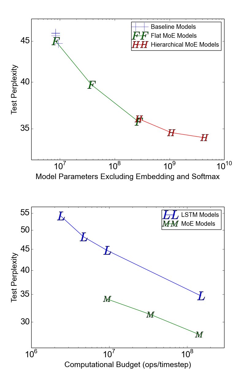
Figure 2: Model comparison on 1-Billion-Word Language-Modeling Benchmark. On the left, we plot test perplexity as a function of model capacity for models with similar computational budgets of approximately 8-million-ops-per-timestep. On the right, we plot test perplexity as a function of computational budget. The top line represents the LSTM models from (Jozefowicz et al., 2016). The bottom line represents 4-billion parameter MoE models with different computational budgets.

图 2：10 亿词语言建模基准上的模型比较。左侧画出计算预算相近（约每时间步 800 万次运算）的模型，测试困惑度随模型容量的变化。右侧画出测试困惑度随计算预算的变化。上方那条线是 Jozefowicz 等（2016）的 LSTM 模型。下方那条线是 40 亿参数、不同计算预算的 MoE 模型。

	Test	Test	#Parameters	ops/timestep	Training	TFLOPS
	Perplexity	Perplexity	excluding embedding		Time	/GPU
	10 epochs	100 epochs	and softmax layers		10 epochs
Best Published Results	34.7	30.6	151 million	151 million	59 hours, 32 k40s	1.09
Low-Budget MoE Model	34.1		4303 million	8.9 million	15 hours, 16 k40s	0.74
Medium-Budget MoE Model	31.3		4313 million	33.8 million	17 hours, 32 k40s	1.22
High-Budget MoE Model	28.0		4371 million	142.7 million	47 hours, 32 k40s	1.56

Table 1: Summary of high-capacity MoE-augmented models with varying computational budgets, vs. best previously published results (Jozefowicz et al., 2016). Details in Appendix C.

	测试	测试	参数量	ops/timestep	训练	TFLOPS
	困惑度	困惑度	不含嵌入		时间	/GPU
	10 个周期	100 个周期	与 softmax 层		10 个周期
此前发表的最好结果	34.7	30.6	151 million	151 million	59 hours, 32 k40s	1.09
低预算 MoE 模型	34.1		4303 million	8.9 million	15 hours, 16 k40s	0.74
中预算 MoE 模型	31.3		4313 million	33.8 million	17 hours, 32 k40s	1.22
高预算 MoE 模型	28.0		4371 million	142.7 million	47 hours, 32 k40s	1.56

表 1：不同计算预算的高容量 MoE 增强模型摘要，对比此前发表的最好结果（Jozefowicz 等，2016）。细节见附录 C。

Varied Computation, High Capacity:

In addition to the largest model from the previous section, we trained two more MoE models with similarly high capacity (4 billion parameters), but higher computation budgets. These models had larger LSTMs, and fewer but larger and experts. Details can be found in Appendix C.2. Results of these three models form the bottom line of Figure 2-right. Table 1 compares the results of these models to the best previously-published result on this dataset . Even the fastest of these models beats the best published result (when controlling for the number of training epochs), despite requiring only 6% of the computation.

变化计算量、高容量：

除上一节中最大的模型外，我们还训练了另外两个容量同样很高（40 亿参数）、但计算预算更高的 MoE 模型。这些模型有更大的 LSTM，以及更少但更大的专家。细节见附录 C.2。这三个模型的结果构成图 2 右侧下方那条线。表 1 把这些模型的结果与该数据集上此前发表的最好结果相比较。即便其中最快的模型，在控制训练周期数后也超过了此前发表的最好结果，尽管只需 6% 的计算量。

Computational Efficiency:

We trained our models using TensorFlow (Abadi et al., 2016) on clusters containing 16-32 Tesla K40 GPUs. For each of our models, we determine computational efficiency in TFLOPS/GPU by dividing the number of floating point operations required to process one training batch by the observed step time and the number of GPUs in the cluster. The operation counts used here are higher than the ones we report in our ops/timestep numbers in that we include the backwards pass, we include the importance-sampling-based training of the softmax layer, and we count a multiply-and-add as two separate operations. For all of our MoE models, the floating point operations involved in the experts represent between 37% and 46% of the total.

计算效率：

我们用 TensorFlow（Abadi 等，2016）在含 16–32 块 Tesla K40 GPU 的集群上训练模型。对每个模型，我们用处理一个训练批次所需的浮点运算次数，除以观测到的步进时间与集群中的 GPU 数，得到以 TFLOPS/GPU 计的计算效率。这里使用的运算计数高于我们在 ops/timestep 中报告的数字：我们计入反向过程，计入基于重要性采样的 softmax 层训练，并把一次乘加计为两次独立运算。对我们所有的 MoE 模型，专家中的浮点运算占总运算的 37% 到 46%。

For our baseline models wtih no MoE, observed computational efficiency ranged from 1.07-1.29 TFLOPS/GPU. For our low-computation MoE models, computation efficiency ranged from 0.74-0.90 TFLOPS/GPU, except for the 4-expert model which did not make full use of the available parallelism. Our highest-computation MoE model was more efficient at 1.56 TFLOPS/GPU, likely due to the larger matrices. These numbers represent a significant fraction of the theoretical maximum of 4.29 TFLOPS/GPU claimed by NVIDIA. Detailed results are in Appendix C, Table 7.

对我们没有 MoE 的基线模型，观测到的计算效率在 1.07–1.29 TFLOPS/GPU。对低计算量 MoE 模型，计算效率在 0.74–0.90 TFLOPS/GPU，但 4 专家模型没有充分利用可用并行性。计算量最高的 MoE 模型更高效，达到 1.56 TFLOPS/GPU，可能是因为矩阵更大。这些数字占 NVIDIA 宣称的理论最大值 4.29 TFLOPS/GPU 的相当一部分。详细结果见附录 C 表 7。

5.2 100 Billion Word Google News Corpus

5.2 1000 亿词的 Google 新闻语料

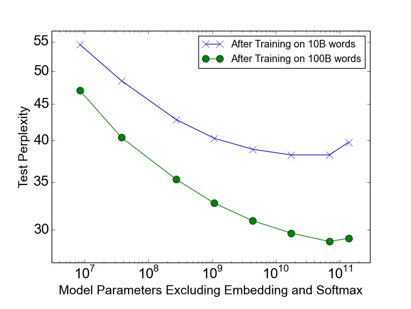
Figure 3: Language modeling on a 100 billion word corpus. Models have similar computational budgets (8 million ops/timestep).

图 3：在 1000 亿词语料上的语言建模。各模型计算预算相近（每时间步 800 万次运算）。

On the 1-billion-word corpus, adding additional capacity seems to produce diminishing returns as the number of parameters in the MoE layer exceeds 1 billion, as can be seen in Figure 2-left. We hypothesized that for a larger training set, even higher capacities would produce significant quality improvements.

在 10 亿词语料上，当 MoE 层参数超过 10 亿后，继续增加容量似乎带来递减的回报，见图 2 左侧。我们猜想，对更大的训练集，更高的容量仍会带来显著的质量改进。

We constructed a similar training set consisting of shuffled unique sentences from Google’s internal news corpus, totalling roughly 100 billion words. Similarly to the previous section, we tested a series of models with similar computational costs of about 8 million ops/timestep. In addition to a baseline LSTM model, we trained models augmented with MoE layers containing 32, 256, 1024, 4096, 16384, 65536, and 131072 experts. This corresponds to up to 137 billion parameters in the MoE layer. Details on architecture, training, and results are given in Appendix D.

我们构建了一个类似的训练集，由 Google 内部新闻语料中打乱的不重复句子组成，总计约 1000 亿词。与上一节类似，我们测试了一系列计算代价相近、约每时间步 800 万次运算的模型。除一个基线 LSTM 模型外，我们训练了 MoE 层分别含 32、256、1024、4096、16384、65536 与 131072 个专家的增强模型。这对应于 MoE 层中最多 1370 亿参数。结构、训练与结果细节见附录 D。

Results:

Figure 3 shows test perplexity as a function of capacity after training on 10 billion words (top line) and 100 billion words (bottom line). When training over the full 100 billion words, test perplexity improves significantly up to 65536 experts (68 billion parameters), dropping 39% lower than the computationally matched baseline, but degrades at 131072 experts, possibly a result of too much sparsity. The widening gap between the two lines demonstrates (unsurprisingly) that increased model capacity helps more on larger training sets.

结果：

图 3 画出在 100 亿词（上方那条线）与 1000 亿词（下方那条线）上训练后，测试困惑度随容量的变化。在全部 1000 亿词上训练时，测试困惑度一直显著改进到 65536 个专家（680 亿参数），比计算量匹配的基线低 39%，但在 131072 个专家时变差，可能是稀疏过度的结果。两条线之间逐渐拉大的差距表明（并不意外）：更大的训练集上，增加模型容量帮助更大。

Even at 65536 experts (99.994% layer sparsity), computational efficiency for the model stays at a respectable 0.72 TFLOPS/GPU.

即便在 65536 个专家（层稀疏度 99.994%）时，该模型的计算效率仍保持在可观的 0.72 TFLOPS/GPU。

5.3 Machine Translation (Single Language Pair)

5.3 机器翻译（单一语言对）

Model Architecture:

Our model was a modified version of the GNMT model described in (Wu et al., 2016). To reduce computation, we decreased the number of LSTM layers in the encoder and decoder from 9 and 8 to 3 and 2 respectively. We inserted MoE layers in both the encoder (between layers 2 and 3) and the decoder (between layers 1 and 2). Each MoE layer contained up to 2048 experts each with about two million parameters, adding a total of about 8 billion parameters to the models. Further details on model architecture, testing procedure and results can be found in Appendix E.

模型结构：

我们的模型是对 Wu 等（2016）所描述的 GNMT 模型的修改版本。为减少计算量，我们把编码器与解码器中的 LSTM 层数分别从 9 与 8 减到 3 与 2。我们在编码器（第 2 层与第 3 层之间）和解码器（第 1 层与第 2 层之间）都插入了 MoE 层。每个 MoE 层最多含 2048 个专家，每个专家约有 200 万参数，总共给模型增加约 80 亿参数。模型结构、测试流程与结果的更多细节见附录 E。

Datasets:

We benchmarked our method on the WMT’14 En$\rightarrow$Fr and En$\rightarrow$De corpora, whose training sets have 36M sentence pairs and 5M sentence pairs, respectively. The experimental protocols were also similar to those in (Wu et al., 2016): newstest2014 was used as the test set to compare against previous work (Luong et al., 2015a; Zhou et al., 2016; Wu et al., 2016), while the combination of newstest2012 and newstest2013 was used as the development set. We also tested the same model on a Google’s Production English to French data.

数据集：

我们在 WMT’14 En$\rightarrow$Fr 与 En$\rightarrow$De 语料上评测，其训练集分别有 3600 万与 500 万句对。实验协议也与 Wu 等（2016）相近：用 newstest2014 作为测试集，以便与先前工作比较（Luong 等，2015a；Zhou 等，2016；Wu 等，2016），用 newstest2012 与 newstest2013 的合并作为开发集。我们还在 Google 的生产英译法语料上测试了同一模型。

Model	Test	Test	ops/timenstep	Total	Training
	Perplexity	BLEU		#Parameters	Time
MoE with 2048 Experts	2.69	40.35	85M	8.7B	3 days/64 k40s
MoE with 2048 Experts (longer training)	2.63	40.56	85M	8.7B	6 days/64 k40s
GNMT (Wu et al., 2016)	2.79	39.22	214M	278M	6 days/96 k80s
GNMT+RL (Wu et al., 2016)	2.96	39.92	214M	278M	6 days/96 k80s
PBMT (Durrani et al., 2014)		37.0
LSTM (6-layer) (Luong et al., 2015b)		31.5
LSTM (6-layer+PosUnk) (Luong et al., 2015b)		33.1
DeepAtt (Zhou et al., 2016)		37.7
DeepAtt+PosUnk (Zhou et al., 2016)		39.2

Table 2: Results on WMT’14 En$\rightarrow$ Fr newstest2014 (bold values represent best results).

模型	测试	测试	ops/timenstep	总计	训练
	困惑度	BLEU		参数量	时间
含 2048 个专家的 MoE	2.69	40.35	85M	8.7B	3 days/64 k40s
含 2048 个专家的 MoE（更长训练）	2.63	40.56	85M	8.7B	6 days/64 k40s
GNMT (Wu et al., 2016)	2.79	39.22	214M	278M	6 days/96 k80s
GNMT+RL (Wu et al., 2016)	2.96	39.92	214M	278M	6 days/96 k80s
PBMT (Durrani et al., 2014)		37.0
LSTM (6-layer) (Luong et al., 2015b)		31.5
LSTM (6-layer+PosUnk) (Luong et al., 2015b)		33.1
DeepAtt (Zhou et al., 2016)		37.7
DeepAtt+PosUnk (Zhou et al., 2016)		39.2

表 2：WMT’14 En$\rightarrow$ Fr newstest2014 上的结果（粗体表示最好结果）。

Model	Test	Test	ops/timestep	Total	Training
	Perplexity	BLEU		#Parameters	Time
MoE with 2048 Experts	4.64	26.03	85M	8.7B	1 day/64 k40s
GNMT (Wu et al., 2016)	5.25	24.91	214M	278M	1 day/96 k80s
GNMT +RL (Wu et al., 2016)	8.08	24.66	214M	278M	1 day/96 k80s
PBMT (Durrani et al., 2014)		20.7
DeepAtt (Zhou et al., 2016)		20.6

Table 3: Results on WMT’14 En $\rightarrow$ De newstest2014 (bold values represent best results).

模型	测试	测试	ops/timestep	总计	训练
	困惑度	BLEU		参数量	时间
含 2048 个专家的 MoE	4.64	26.03	85M	8.7B	1 day/64 k40s
GNMT (Wu et al., 2016)	5.25	24.91	214M	278M	1 day/96 k80s
GNMT +RL (Wu et al., 2016)	8.08	24.66	214M	278M	1 day/96 k80s
PBMT (Durrani et al., 2014)		20.7
DeepAtt (Zhou et al., 2016)		20.6

表 3：WMT’14 En $\rightarrow$ De newstest2014 上的结果（粗体表示最好结果）。

Model	Eval	Eval	Test	Test	ops/timestep	Total	Training
	Perplexity	BLEU	Perplexity	BLEU		#Parameters	Time
MoE with 2048 Experts	2.60	37.27	2.69	36.57	85M	8.7B	1 day/64 k40s
GNMT (Wu et al., 2016)	2.78	35.80	2.87	35.56	214M	278M	6 days/96 k80s

Table 4: Results on the Google Production En$\rightarrow$ Fr dataset (bold values represent best results).

模型	评估	评估	测试	测试	ops/timestep	总计	训练
	困惑度	BLEU	困惑度	BLEU		参数量	时间
含 2048 个专家的 MoE	2.60	37.27	2.69	36.57	85M	8.7B	1 day/64 k40s
GNMT (Wu et al., 2016)	2.78	35.80	2.87	35.56	214M	278M	6 days/96 k80s

表 4：Google 生产 En$\rightarrow$ Fr 数据集上的结果（粗体表示最好结果）。

Results:

Tables 2, 3, and  4 show the results of our largest models, compared with published results. Our approach achieved BLEU scores of 40.56 and 26.03 on the WMT’14 En$\rightarrow$Fr and En$\rightarrow$De benchmarks. As our models did not use RL refinement, these results constitute significant gains of 1.34 and 1.12 BLEU score on top of the strong baselines in (Wu et al., 2016). The perplexity scores are also better.[^2] On the Google Production dataset, our model achieved 1.01 higher test BLEU score even after training for only one sixth of the time.

结果：

表 2、3 与 4 给出我们最大模型的结果，并与已发表结果比较。我们的方法在 WMT’14 En$\rightarrow$Fr 与 En$\rightarrow$De 基准上分别取得 40.56 与 26.03 的 BLEU。由于我们的模型没有使用强化学习精炼，这些结果相对 Wu 等（2016）中的强基线分别显著提高了 1.34 与 1.12 BLEU。困惑度也更好。[^2] 在 Google 生产数据集上，即便只训练了六分之一的时间，我们的模型测试 BLEU 仍高出 1.01。

5.4 Multilingual Machine Translation

5.4 多语言机器翻译

Dataset:

(Johnson et al., 2016) train a single GNMT (Wu et al., 2016) model on a very large combined dataset of twelve language pairs. Results are somewhat worse than those for 12 separately trained single-pair GNMT models. This is not surprising, given that the twelve models have 12 times the capacity and twelve times the aggregate training of the one model. We repeat this experiment with a single MoE-augmented model. See Appendix E for details on model architecture. We train our model on the same dataset as (Johnson et al., 2016) and process the same number of training examples (about 3 billion sentence pairs). Our training time was shorter due to the lower computational budget of our model.

数据集：

Johnson 等（2016）在由十二个语言对组成的很大合并数据集上训练单个 GNMT（Wu 等，2016）模型。结果略差于分别训练的 12 个单语对 GNMT 模型。这并不令人意外，因为那十二个模型的容量是单个模型的 12 倍，合计训练量也是 12 倍。我们用单个 MoE 增强模型重复这一实验。模型结构细节见附录 E。我们在与 Johnson 等（2016）相同的数据集上训练，并处理相同数量的训练样本（约 30 亿句对）。由于我们模型的计算预算更低，训练时间更短。

Results:

Results for the single-pair GNMT models, the multilingual GNMT model and the multilingual MoE model are given in Table 5. The MoE model achieves 19% lower perplexity on the dev set than the multilingual GNMT model. On BLEU score, the MoE model significantly beats the multilingual GNMT model on 11 of the 12 language pairs (by as much as 5.84 points), and even beats the monolingual GNMT models on 8 of 12 language pairs. The poor performance on English $\rightarrow$ Korean seems to be a result of severe overtraining, as for the rarer language pairs a small number of real examples were highly oversampled in the training corpus.

结果：

单语对 GNMT 模型、多语言 GNMT 模型与多语言 MoE 模型的结果见表 5。MoE 模型在开发集上的困惑度比多语言 GNMT 模型低 19%。在 BLEU 上，MoE 模型在 12 个语言对中的 11 个上显著超过多语言 GNMT 模型（最多高出 5.84 分），甚至在 12 个语言对中的 8 个上超过单语 GNMT 模型。英语 $\rightarrow$ 韩语上的较差表现似乎是严重过训练的结果，因为对较稀有的语言对，训练语料中少量真实样本被高度过采样。

	GNMT-Mono	GNMT-Multi	MoE-Multi	MoE-Multi vs.
				GNMT-Multi
Parameters	278M / model	278M	8.7B
ops/timestep	212M	212M	102M
training time, hardware	various	21 days, 96 k20s	12 days, 64 k40s
Perplexity (dev)		4.14	3.35	-19%
French $\rightarrow$ English Test BLEU	36.47	34.40	37.46	+3.06
German $\rightarrow$ English Test BLEU	31.77	31.17	34.80	+3.63
Japanese $\rightarrow$ English Test BLEU	23.41	21.62	25.91	+4.29
Korean $\rightarrow$ English Test BLEU	25.42	22.87	28.71	+5.84
Portuguese $\rightarrow$ English Test BLEU	44.40	42.53	46.13	+3.60
Spanish $\rightarrow$ English Test BLEU	38.00	36.04	39.39	+3.35
English $\rightarrow$ French Test BLEU	35.37	34.00	36.59	+2.59
English $\rightarrow$ German Test BLEU	26.43	23.15	24.53	+1.38
English $\rightarrow$ Japanese Test BLEU	23.66	21.10	22.78	+1.68
English $\rightarrow$ Korean Test BLEU	19.75	18.41	16.62	-1.79
English $\rightarrow$ Portuguese Test BLEU	38.40	37.35	37.90	+0.55
English $\rightarrow$ Spanish Test BLEU	34.50	34.25	36.21	+1.96

Table 5: Multilingual Machine Translation (bold values represent best results).

	GNMT-Mono	GNMT-Multi	MoE-Multi	MoE-Multi vs.
				GNMT-Multi
参数量	278M / model	278M	8.7B
ops/timestep	212M	212M	102M
训练时间与硬件	various	21 days, 96 k20s	12 days, 64 k40s
困惑度（开发集）		4.14	3.35	-19%
French $\rightarrow$ English 测试 BLEU	36.47	34.40	37.46	+3.06
German $\rightarrow$ English 测试 BLEU	31.77	31.17	34.80	+3.63
Japanese $\rightarrow$ English 测试 BLEU	23.41	21.62	25.91	+4.29
Korean $\rightarrow$ English 测试 BLEU	25.42	22.87	28.71	+5.84
Portuguese $\rightarrow$ English 测试 BLEU	44.40	42.53	46.13	+3.60
Spanish $\rightarrow$ English 测试 BLEU	38.00	36.04	39.39	+3.35
English $\rightarrow$ French 测试 BLEU	35.37	34.00	36.59	+2.59
English $\rightarrow$ German 测试 BLEU	26.43	23.15	24.53	+1.38
English $\rightarrow$ Japanese 测试 BLEU	23.66	21.10	22.78	+1.68
English $\rightarrow$ Korean 测试 BLEU	19.75	18.41	16.62	-1.79
English $\rightarrow$ Portuguese 测试 BLEU	38.40	37.35	37.90	+0.55
English $\rightarrow$ Spanish 测试 BLEU	34.50	34.25	36.21	+1.96

表 5：多语言机器翻译（粗体表示最好结果）。

6 Conclusion

6 结论

This work is the first to demonstrate major wins from conditional computation in deep networks. We carefully identified the design considerations and challenges of conditional computing and addressed them with a combination of algorithmic and engineering solutions. While we focused on text, conditional computation may help in other domains as well, provided sufficiently large training sets. We look forward to seeing many novel implementations and applications of conditional computation in the years to come.

这项工作首次表明，条件计算可以在深度网络中带来重大收益。我们仔细厘清了条件计算的设计考量与挑战，并用算法与工程方案的组合加以应对。虽然我们关注文本，但只要训练集足够大，条件计算也可能在其他领域有帮助。我们期待在未来若干年里看到条件计算的许多新实现与新应用。

Acknowledgments

We would like to thank all of the members of the Google Brain and Google Translate teams who helped us with this project, in particular Zhifeng Chen, Yonghui Wu, and Melvin Johnson. Thanks also to our anonymous ICLR reviewers for the helpful suggestions on making this paper better.

致谢

我们感谢 Google Brain 与 Google 翻译团队中帮助过本项目的所有成员，尤其是 Zhifeng Chen、Yonghui Wu 与 Melvin Johnson。也感谢匿名 ICLR 审稿人就改进本文提出的有益建议。

References

Abadi et al. (2016) Martín Abadi, Ashish Agarwal, Paul Barham, Eugene Brevdo, Zhifeng Chen, Craig Citro, Gregory S. Corrado, Andy Davis, Jeffrey Dean, Matthieu Devin, Sanjay Ghemawat, Ian J. Goodfellow, Andrew Harp, Geoffrey Irving, Michael Isard, Yangqing Jia, Rafal Józefowicz, Lukasz Kaiser, Manjunath Kudlur, Josh Levenberg, Dan Mané, Rajat Monga, Sherry Moore, Derek Gordon Murray, Chris Olah, Mike Schuster, Jonathon Shlens, Benoit Steiner, Ilya Sutskever, Kunal Talwar, Paul A. Tucker, Vincent Vanhoucke, Vijay Vasudevan, Fernanda B. Viégas, Oriol Vinyals, Pete Warden, Martin Wattenberg, Martin Wicke, Yuan Yu, and Xiaoqiang Zheng. Tensorflow: Large-scale machine learning on heterogeneous distributed systems. CoRR , abs/1603.04467, 2016. URL http://arxiv.org/abs/1603.04467 .

Aljundi et al. (2016) Rahaf Aljundi, Punarjay Chakravarty, and Tinne Tuytelaars. Expert gate: Lifelong learning with a network of experts. CoRR , abs/1611.06194, 2016. URL http://arxiv.org/abs/1611.06194 .

Almahairi et al. (2015) A. Almahairi, N. Ballas, T. Cooijmans, Y. Zheng, H. Larochelle, and A. Courville. Dynamic Capacity Networks. ArXiv e-prints , November 2015.

Amodei et al. (2015) Dario Amodei, Rishita Anubhai, Eric Battenberg, Carl Case, Jared Casper, Bryan Catanzaro, Jingdong Chen, Mike Chrzanowski, Adam Coates, Greg Diamos, Erich Elsen, Jesse Engel, Linxi Fan, Christopher Fougner, Tony Han, Awni Y. Hannun, Billy Jun, Patrick LeGresley, Libby Lin, Sharan Narang, Andrew Y. Ng, Sherjil Ozair, Ryan Prenger, Jonathan Raiman, Sanjeev Satheesh, David Seetapun, Shubho Sengupta, Yi Wang, Zhiqian Wang, Chong Wang, Bo Xiao, Dani Yogatama, Jun Zhan, and Zhenyao Zhu. Deep speech 2: End-to-end speech recognition in english and mandarin. arXiv preprint arXiv:1512.02595 , 2015.

Bahdanau et al. (2014) Dzmitry Bahdanau, Kyunghyun Cho, and Yoshua Bengio. Neural machine translation by jointly learning to align and translate. arXiv preprint arXiv:1409.0473 , 2014.

Bengio et al. (2015) Emmanuel Bengio, Pierre-Luc Bacon, Joelle Pineau, and Doina Precup. Conditional computation in neural networks for faster models. arXiv preprint arXiv:1511.06297 , 2015.

Bengio et al. (2013) Yoshua Bengio, Nicholas Léonard, and Aaron Courville. Estimating or propagating gradients through stochastic neurons for conditional computation. arXiv preprint arXiv:1308.3432 , 2013.

Chelba et al. (2013) Ciprian Chelba, Tomas Mikolov, Mike Schuster, Qi Ge, Thorsten Brants, Phillipp Koehn, and Tony Robinson. One billion word benchmark for measuring progress in statistical language modeling. arXiv preprint arXiv:1312.3005 , 2013.

Cho & Bengio (2014) K. Cho and Y. Bengio. Exponentially Increasing the Capacity-to-Computation Ratio for Conditional Computation in Deep Learning. ArXiv e-prints , June 2014.

Collobert et al. (2002) Ronan Collobert, Samy Bengio, and Yoshua Bengio. A parallel mixture of SVMs for very large scale problems. Neural Computing , 2002.

Davis & Arel (2013) Andrew Davis and Itamar Arel. Low-rank approximations for conditional feedforward computation in deep neural networks. arXiv preprint arXiv:1312.4461 , 2013.

Deisenroth & Ng (2015) Marc Peter Deisenroth and Jun Wei Ng. Distributed Gaussian processes. In ICML , 2015.

Duchi et al. (2010) John Duchi, Elad Hazan, and Yoram Singer. Adaptive subgradient methods for online learning and stochastic optimization, 2010.

Durrani et al. (2014) Nadir Durrani, Barry Haddow, Philipp Koehn, and Kenneth Heafield. Edinburgh’s phrase-based machine translation systems for wmt-14. In Proceedings of the Ninth Workshop on Statistical Machine Translation , 2014.

Eigen et al. (2013) David Eigen, Marc’Aurelio Ranzato, and Ilya Sutskever. Learning factored representations in a deep mixture of experts. arXiv preprint arXiv:1312.4314 , 2013.

Garmash & Monz (2016) Ekaterina Garmash and Christof Monz. Ensemble learning for multi-source neural machine translation. In staff.science.uva.nl/c.monz , 2016.

Gers et al. (2000) Felix A. Gers, Jürgen A. Schmidhuber, and Fred A. Cummins. Learning to forget: Continual prediction with lstm. Neural Computation , 2000.

Gruslys et al. (2016) Audrunas Gruslys, Rémi Munos, Ivo Danihelka, Marc Lanctot, and Alex Graves. Memory-efficient backpropagation through time. CoRR , abs/1606.03401, 2016. URL http://arxiv.org/abs/1606.03401 .

He et al. (2015) Kaiming He, Xiangyu Zhang, Shaoqing Ren, and Jian Sun. Deep residual learning for image recognition. IEEE Conference on Computer Vision and Pattern Recognition , 2015.

Hinton et al. (2012) Geoffrey Hinton, Li Deng, Dong Yu, George E. Dahl, Abdel-rahman Mohamed, Navdeep Jaitly, Andrew Senior, Vincent Vanhoucke, Patrick Nguyen, Tara N. Sainath, et al. Deep neural networks for acoustic modeling in speech recognition: The shared views of four research groups. IEEE Signal Processing Magazine , 2012.

Hochreiter & Schmidhuber (1997) Sepp Hochreiter and Jürgen Schmidhuber. Long short-term memory. Neural Computation , 1997.

Ioffe & Szegedy (2015) Sergey Ioffe and Christian Szegedy. Batch normalization: Accelerating deep network training by reducing internal covariate shift. arXiv preprint arXiv:1502.03167 , 2015.

Jacobs et al. (1991) Robert A. Jacobs, Michael I. Jordan, Steven J. Nowlan, and Geoffrey E. Hinton. Adaptive mixtures of local experts. Neural Computing , 1991.

Johnson et al. (2016) Melvin Johnson, Mike Schuster, Quoc V. Le, Maxim Krikun, Yonghui Wu, Zhifeng Chen, Nikhil Thorat, Fernanda B. Viégas, Martin Wattenberg, Greg Corrado, Macduff Hughes, and Jeffrey Dean. Google’s multilingual neural machine translation system: Enabling zero-shot translation. CoRR , abs/1611.04558, 2016. URL http://arxiv.org/abs/1611.04558 .

Jordan & Jacobs (1994) Michael I. Jordan and Robert A. Jacobs. Hierarchical mixtures of experts and the EM algorithm. Neural Computing , 1994.

Jozefowicz et al. (2016) Rafal Jozefowicz, Oriol Vinyals, Mike Schuster, Noam Shazeer, and Yonghui Wu. Exploring the limits of language modeling. arXiv preprint arXiv:1602.02410 , 2016.

Kingma & Ba (2015) Diederik Kingma and Jimmy Ba. Adam: A method for stochastic optimization. In ICLR , 2015.

Kneser & Ney (1995) Reinhard Kneser and Hermann. Ney. Improved backingoff for m-gram language modeling., 1995.

Krizhevsky et al. (2012) Alex Krizhevsky, Ilya Sutskever, and Geoffrey E. Hinton. Imagenet classification with deep convolutional neural networks. In NIPS , 2012.

Le et al. (2012) Quoc V. Le, Marc’Aurelio Ranzato, Rajat Monga, Matthieu Devin, Kai Chen, Greg S. Corrado, Jeffrey Dean, and Andrew Y. Ng. Building high-level features using large scale unsupervised learning. In ICML , 2012.

Ludovic Denoyer (2014) Patrick Gallinari Ludovic Denoyer. Deep sequential neural network. arXiv preprint arXiv:1410.0510 , 2014.

Luong et al. (2015a) Minh-Thang Luong, Hieu Pham, and Christopher D. Manning. Effective approaches to attention-based neural machine translation. EMNLP , 2015a.

Luong et al. (2015b) Minh-Thang Luong, Ilya Sutskever, Quoc V. Le, Oriol Vinyals, and Wojciech Zaremba. Addressing the rare word problem in neural machine translation. ACL , 2015b.

Rasmussen & Ghahramani (2002) Carl Edward Rasmussen and Zoubin Ghahramani. Infinite mixtures of Gaussian process experts. NIPS , 2002.

Sak et al. (2014) Hasim Sak, Andrew W Senior, and Françoise Beaufays. Long short-term memory recurrent neural network architectures for large scale acoustic modeling. In INTERSPEECH , pp. 338–342, 2014.

Schuster & Nakajima (2012) Mike Schuster and Kaisuke Nakajima. Japanese and Korean voice search. ICASSP , 2012.

Shahbaba & Neal (2009) Babak Shahbaba and Radford Neal. Nonlinear models using dirichlet process mixtures. JMLR , 2009.

Sutskever et al. (2014) Ilya Sutskever, Oriol Vinyals, and Quoc V. Le. Sequence to sequence learning with neural networks. In NIPS , 2014.

Theis & Bethge (2015) Lucas Theis and Matthias Bethge. Generative image modeling using spatial LSTMs. In NIPS , 2015.

Tresp (2001) Volker Tresp. Mixtures of Gaussian Processes. In NIPS , 2001.

Wu et al. (2016) Yonghui Wu, Mike Schuster, Zhifeng Chen, Quoc V. Le, Mohammad Norouzi, Wolfgang Macherey, Maxim Krikun, Yuan Cao, Qin Gao, Klaus Macherey, Jeff Klingner, Apurva Shah, Melvin Johnson, Xiaobing Liu, Łukasz Kaiser, Stephan Gouws, Yoshikiyo Kato, Taku Kudo, Hideto Kazawa, Keith Stevens, George Kurian, Nishant Patil, Wei Wang, Cliff Young, Jason Smith, Jason Riesa, Alex Rudnick, Oriol Vinyals, Greg Corrado, Macduff Hughes, and Jeffrey Dean. Google’s neural machine translation system: Bridging the gap between human and machine translation. arXiv preprint arXiv:1609.08144 , 2016.

Yao et al. (2009) Bangpeng Yao, Dirk Walther, Diane Beck, and Li Fei-fei. Hierarchical mixture of classification experts uncovers interactions between brain regions. In NIPS . 2009.

Zaremba et al. (2014) Wojciech Zaremba, Ilya Sutskever, and Oriol Vinyals. Recurrent neural network regularization. arXiv preprint arXiv:1409.2329 , 2014.

Zhou et al. (2016) Jie Zhou, Ying Cao, Xuguang Wang, Peng Li, and Wei Xu. Deep recurrent models with fast-forward connections for neural machine translation. arXiv preprint arXiv:1606.04199 , 2016.

Appendices

A Load-Balancing Loss

A 负载均衡损失

As discussed in section 4, for load-balancing purposes, we want to define an additional loss function to encourage experts to receive roughly equal numbers of training examples. Unfortunately, the number of examples received by an expert is a discrete quantity, so it can not be used in back-propagation. Instead, we define a smooth estimator $Load(X)$ of the number of examples assigned to each expert for a batch $X$ of inputs. The smoothness allows us to back-propagate gradients through the estimator. This is the purpose of the noise term in the gating function. We define $P(x,i)$ as the probability that $G(x)_{i}$ is nonzero, given a new random choice of noise on element $i$, but keeping the already-sampled choices of noise on the other elements. To compute $P(x,i)$, we note that the $G(x)_{i}$ is nonzero if and only if $H(x)_{i}$ is greater than the $k^{th}$-greatest element of $H(x)$ excluding itself. The probability works out to be:

如第 4 节所讨论的，出于负载均衡的目的，我们希望定义一个额外的损失函数，以鼓励各专家收到大致相同数量的训练样本。可惜，一个专家收到的样本数是离散量，不能用于反向传播。于是我们定义一个平滑估计量 $Load(X)$，用来估计一批输入 $X$ 中分配给每个专家的样本数。平滑性使我们能够把梯度通过该估计量反向传播。这正是门控函数中噪声项的用途。我们把 $P(x,i)$ 定义为：在对第 $i$ 个元素重新随机抽取噪声、同时保持其他元素已采样噪声不变的条件下，$G(x)_{i}$ 非零的概率。要计算 $P(x,i)$，我们注意到 $G(x)_{i}$ 非零，当且仅当 $H(x)_{i}$ 大于 $H(x)$ 中除去自身后的第 $k$ 大元素。该概率可写成：

$$\displaystyle P(x,i)=Pr\Big((x\cdot W_{g})_{i}+StandardNormal()\cdot Softplus((x\cdot W_{noise})_{i}) \\ \displaystyle>kth\_excluding(H(x),k,i)\Big)$$

Where $kth\_excluding(v,k,i)$ means the kth highest component of $v$, excluding component $i$. Simplifying, we get:

其中 $kth\_excluding(v,k,i)$ 表示 $v$ 中除去第 $i$ 个分量后的第 $k$ 大分量。化简后得到：

$$P(x,i)=\Phi\Big(\frac{(x\cdot W_{g})_{i}-kth\_excluding(H(x),k,i)}{Softplus((x\cdot W_{noise})_{i})}\Big) \tag{9}$$

Where $\Phi$ is the CDF of the standard normal distribution.

其中 $\Phi$ 是标准正态分布的累积分布函数。

$$Load(X)_{i}=\sum_{x\in X}P(x,i) \tag{10}$$

We can now define the load loss to be the square of the coefficient of variation of the load vector, multiplied by a hand-tuned scaling factor $w_{load}$.

现在可以把负载损失定义为负载向量变异系数的平方，再乘以手工调节的缩放因子 $w_{load}$。

$$L_{load}(X)=w_{load}\cdot CV(Load(X))^{2} \tag{11}$$

Initial Load Imbalance:

To avoid out-of-memory errors, we need to initialize the network in a state of approximately equal expert load (since the soft constraints need some time to work). To accomplish this, we initialize the matrices $W_{g}$ and $W_{noise}$ to all zeros, which yields no signal and some noise.

初始负载不均衡：

为避免内存溢出错误，我们需要把网络初始化到专家负载大致相等的状态（因为软约束需要一些时间才能起作用）。为此，我们把矩阵 $W_{g}$ 与 $W_{noise}$ 初始化为全零，从而没有信号、只有一些噪声。

Experiments:

We trained a set of models with identical architecture (the MoE-256 model described in Appendix C), using different values of $w_{importance}$ and $w_{load}$. We trained each model for 10 epochs, then measured perplexity on the test set. We also measured the coefficients of variation in $Importance$ and $Load$, as well as ratio of the load on the most overloaded expert to the average load. This last value is significant for load balancing purposes on distributed hardware. All of these metrics were averaged over several training batches.

实验：

我们用相同结构（附录 C 中描述的 MoE-256 模型）训练一组模型，采用不同的 $w_{importance}$ 与 $w_{load}$。每个模型训练 10 个周期，然后在测试集上测量困惑度。我们还测量了 $Importance$ 与 $Load$ 的变异系数，以及负载最重的专家的负载与平均负载之比。最后一个值对分布式硬件上的负载均衡很重要。这些指标都在若干训练批次上取平均。

$w_{importance}$	$w_{load}$	Test Perplexity	$CV(Importance(X))$	$CV(Load(X))$	$\frac{max(Load(X))}{mean(Load(X))}$
0.0	0.0	39.8	3.04	3.01	17.80
0.2	0.0	35.6	0.06	0.17	1.47
0.0	0.2	35.7	0.22	0.04	1.15
0.1	0.1	35.6	0.06	0.05	1.14
0.01	0.01	35.7	0.48	0.11	1.37
1.0	1.0	35.7	0.03	0.02	1.07

Table 6: Experiments with different combinations of losses.

$w_{importance}$	$w_{load}$	测试困惑度	$CV(Importance(X))$	$CV(Load(X))$	$\frac{max(Load(X))}{mean(Load(X))}$
0.0	0.0	39.8	3.04	3.01	17.80
0.2	0.0	35.6	0.06	0.17	1.47
0.0	0.2	35.7	0.22	0.04	1.15
0.1	0.1	35.6	0.06	0.05	1.14
0.01	0.01	35.7	0.48	0.11	1.37
1.0	1.0	35.7	0.03	0.02	1.07

表 6：不同损失组合的实验。

Results:

Results are reported in Table 6. All the combinations containing at least one the two losses led to very similar model quality, where having no loss was much worse. Models with higher values of $w_{load}$ had lower loads on the most overloaded expert.

结果：

结果见表 6。只要包含两个损失中的至少一个，各组合得到的模型质量都非常接近；完全没有损失则差得多。$w_{load}$ 更大的模型，负载最重的专家上的负载更低。

B Hierachical Mixture of Experts

B 层次化混合专家

If the number of experts is very large, we can reduce the branching factor by using a two-level hierarchical MoE. In a hierarchical MoE, a primary gating network chooses a sparse weighted combination of ‘‘experts", each of which is itself a secondary mixture-of-experts with its own gating network.[^3] If the hierarchical MoE consists of $a$ groups of $b$ experts each, we denote the primary gating network by $G_{primary}$, the secondary gating networks by $(G_{1},G_{2}..G_{a})$, and the expert networks by $(E_{0,0},E_{0,1}..E_{a,b})$. The output of the MoE is given by:

若专家数非常大，我们可以用两级层次化 MoE 来降低分支因子。在层次化 MoE 中，主门控网络选择一个稀疏加权的“专家”组合，而每个“专家”本身又是带有自己门控网络的次级混合专家。[^3] 若层次化 MoE 由 $a$ 组、每组 $b$ 个专家组成，我们把主门控网络记为 $G_{primary}$，次级门控网络记为 $(G_{1},G_{2}..G_{a})$，专家网络记为 $(E_{0,0},E_{0,1}..E_{a,b})$。MoE 的输出为：

$$y_{H}=\sum_{i=1}^{a}\sum_{j=1}^{b}G_{primary}(x)_{i}\cdot G_{i}(x)_{j}\cdot E_{i,j}(x) \tag{12}$$

Our metrics of expert utilization change to the following:

我们的专家利用率指标变为：

$$Importance_{H}(X)_{i,j}=\sum_{x\in X}G_{primary}(x)_{i}\cdot G_{i}(x)_{j} \tag{13}$$

$$Load_{H}(X)_{i,j}=\frac{Load_{primary}(X)_{i}\cdot Load_{i}(X^{(i)})_{j}}{|X^{(i)}|} \tag{14}$$

$Load_{primary}$ and $Load_{i}$ deonte the $Load$ functions for the primary gating network and $i^{th}$ secondary gating network respectively. $X^{(i)}$ denotes the subset of $X$ for which $G_{primary}(x)_{i}>0$.

$Load_{primary}$ 与 $Load_{i}$ 分别表示主门控网络与第 $i$ 个次级门控网络的 $Load$ 函数。$X^{(i)}$ 表示 $X$ 中满足 $G_{primary}(x)_{i}>0$ 的子集。

It would seem simpler to let $Load_{H}(X)_{i,j}=Load_{i}(X_{i})_{j}$ , but this would not have a gradient with respect to the primary gating network, so we use the formulation above.

让 $Load_{H}(X)_{i,j}=Load_{i}(X_{i})_{j}$ 看起来更简单，但这相对于主门控网络没有梯度，因此我们采用上面的写法。

C 1 Billion Word Language Modeling Benchmark - Experimental Details

C 10 亿词语言建模基准——实验细节

Model Architecture:

Our model consists of five layers: a word embedding layer, a recurrent Long Short-Term Memory (LSTM) layer (Hochreiter & Schmidhuber, 1997; Gers et al., 2000), a MoE layer, a second LSTM layer, and a softmax layer. The dimensionality of the embedding layer, the number of units in each LSTM layer, and the input and output dimensionality of the MoE layer are all equal to 512. For every layer other than the softmax, we apply drouput (Zaremba et al., 2014) to the layer output, dropping each activation with probability $DropProb$, otherwise dividing by $(1-DropProb)$. After dropout, the output of the previous layer is added to the layer output. This residual connection encourages gradient flow (He et al., 2015).

模型结构：

我们的模型由五层组成：词嵌入层、一个循环长短期记忆（LSTM）层（Hochreiter 与 Schmidhuber，1997；Gers 等，2000）、一个 MoE 层、第二个 LSTM 层，以及一个 softmax 层。嵌入层的维度、每个 LSTM 层的单元数，以及 MoE 层的输入与输出维度都等于 512。除 softmax 外的每一层，我们对层输出施加 dropout（Zaremba 等，2014），以概率 $DropProb$ 丢弃每个激活，否则除以 $(1-DropProb)$。dropout 之后，把上一层的输出加到本层输出上。这一残差连接有助于梯度流动（He 等，2015）。

MoE Layer Architecture:

Each expert in the MoE layer is a feed forward network with one ReLU-activated hidden layer of size 1024 and an output layer of size 512. Thus, each expert contains $[512*1024]+[1024*512]=1M$ parameters. The output of the MoE layer is passed through a sigmoid function before dropout. We varied the number of experts between models, using ordinary MoE layers with 4, 32 and 256 experts and hierarchical MoE layers with 256, 1024 and 4096 experts. We call the resulting models MoE-4, MoE-32, MoE-256, MoE-256-h, MoE-1024-h and MoE-4096-h. For the hierarchical MoE layers, the first level branching factor was 16, corresponding to the number of GPUs in our cluster. We use Noisy-Top-K Gating (see Section 2.1) with $k=4$ for the ordinary MoE layers and $k=2$ at each level of the hierarchical MoE layers. Thus, each example is processed by exactly 4 experts for a total of 4M ops/timestep. The two LSTM layers contribute 2M ops/timestep each for the desired total of 8M.

MoE 层结构：

MoE 层中的每个专家是一个前馈网络，带一个大小为 1024、ReLU 激活的隐藏层，以及大小为 512 的输出层。因此每个专家含 $[512*1024]+[1024*512]=1M$ 参数。MoE 层的输出在 dropout 之前经过 sigmoid 函数。我们在不同模型之间变化专家数，使用含 4、32 与 256 个专家的普通 MoE 层，以及含 256、1024 与 4096 个专家的层次化 MoE 层。我们把所得模型分别叫做 MoE-4、MoE-32、MoE-256、MoE-256-h、MoE-1024-h 与 MoE-4096-h。对层次化 MoE 层，第一级分支因子为 16，与集群中的 GPU 数对应。我们使用带噪声的 Top-K 门控（见第 2.1 节），普通 MoE 层取 $k=4$，层次化 MoE 层每一级取 $k=2$。因此每个样本恰好由 4 个专家处理，总计每时间步 400 万次运算。两个 LSTM 层各贡献每时间步 200 万次运算，达到期望的总计 800 万。

Computationally-Matched Baselines:

The MoE-4 model does not employ sparsity, since all 4 experts are always used. In addition, we trained four more computationally-matched baseline models with no sparsity:

计算量匹配的基线：

MoE-4 模型不采用稀疏性，因为 4 个专家始终都被使用。此外，我们还训练了另外四个没有稀疏性、计算量匹配的基线模型：

• • MoE-1-Wide: The MoE layer consists of a single "expert" containing one ReLU-activated hidden layer of size 4096.

• • MoE-1-Wide：MoE 层由单个“专家”组成，该专家含一个大小为 4096、ReLU 激活的隐藏层。

• • MoE-1-Deep: The MoE layer consists of a single "expert" containing four ReLU-activated hidden layers, each with size $1024$.

• • MoE-1-Deep：MoE 层由单个“专家”组成，该专家含四个 ReLU 激活的隐藏层，每个大小为 $1024$。

• • 4xLSTM-512: We replace the MoE layer with two additional 512-unit LSTM layers.

• • 4xLSTM-512：我们用另外两个 512 单元的 LSTM 层替换 MoE 层。

• • LSTM-2048-512: The model contains one 2048-unit LSTM layer (and no MoE). The output of the LSTM is projected down to 512 dimensions (Sak et al., 2014). The next timestep of the LSTM receives the projected output. This is identical to one of the models published in (Jozefowicz et al., 2016). We re-ran it to account for differences in training regimen, and obtained results very similar to the published ones.

• • LSTM-2048-512：模型含一个 2048 单元的 LSTM 层（没有 MoE）。LSTM 的输出被投影到 512 维（Sak 等，2014）。LSTM 的下一时间步接收投影后的输出。这与 Jozefowicz 等（2016）发表的模型之一相同。我们重新跑了一遍以计入训练安排的差异，得到的结果与已发表结果非常接近。

Training:

The models were trained on a cluster of 16 K40 GPUs using the synchronous method described in Section 3. Each batch consisted of a set of sentences totaling roughly 300,000 words. In the interest of time, we limited training to 10 epochs, (27,000 steps). Training took 12-16 hours for all models, except for MoE-4, which took 18 hours (since all the expert computation was performed on only 4 of 16 GPUs). We used the Adam optimizer (Kingma & Ba, 2015). The base learning rate was increased linearly for the first 1000 training steps, and decreased after that so as to be proportional to the inverse square root of the step number. The Softmax output layer was trained efficiently using importance sampling similarly to the models in (Jozefowicz et al., 2016). For each model, we performed a hyper-parmeter search to find the best dropout probability, in increments of 0.1.

训练：

模型在 16 块 K40 GPU 的集群上，用第 3 节描述的同步方法训练。每个批次由总计约 30 万词的一组句子组成。出于时间考虑，我们把训练限制在 10 个周期（27,000 步）。除 MoE-4 用了 18 小时（因为全部专家计算只在 16 块 GPU 中的 4 块上执行）外，所有模型的训练时间为 12–16 小时。我们使用 Adam 优化器（Kingma 与 Ba，2015）。基础学习率在前 1000 个训练步线性增加，之后按步数平方根的倒数下降。Softmax 输出层用与 Jozefowicz 等（2016）模型类似的重要性采样高效训练。对每个模型，我们以 0.1 为步长搜索超参数，以找到最好的 dropout 概率。

To ensure balanced expert utilization we set $w_{importance}=0.1$ and $w_{load}=0.1$, as described in Section 4 and Appendix A.

为保证专家利用率均衡，我们按第 4 节与附录 A 所述，设 $w_{importance}=0.1$ 与 $w_{load}=0.1$。

Results:

We evaluate our model using perplexity on the holdout dataset, used by (Chelba et al., 2013; Jozefowicz et al., 2016). We follow the standard procedure and sum over all the words including the end of sentence symbol. Results are reported in Table 7. For each model, we report the test perplexity, the computational budget, the parameter counts, the value of $DropProb$, and the computational efficiency.

结果：

我们用 Chelba 等（2013）与 Jozefowicz 等（2016）使用的留出数据集上的困惑度来评估模型。我们遵循标准做法，对包括句末符号在内的所有词求和。结果见表 7。对每个模型，我们报告测试困惑度、计算预算、参数量、$DropProb$ 的取值以及计算效率。

Model	Test	Test	ops/timestep	#Params excluding	Total	$Drop$-	TFLOPS
	Perplexity	Perplexity	(millions)	embed. & softmax	#Params	$Prob$	per GPU
	10 epochs	(final)		(millions)	(billions)		(observed)
Kneser-Ney 5-gram*		67.6	0.00001		1.8
LSTM-512-512*		54.1	2.4	2.4	0.8	0.1
LSTM-1024-512*		48.2	4.7	4.7	0.8	0.1
LSTM-2048-512*	45.0	43.7	9.4	9.4	0.8	0.1	0.61
LSTM-2048-512	44.7		9.4	9.4	0.8	0.1	1.21
4xLSTM-512	46.0		8.4	8.4	0.8	0.1	1.07
MoE-1-Wide	46.1		8.4	8.4	0.8	0.1	1.29
MoE-1-Deep	45.7		8.4	8.4	0.8	0.1	1.29
MoE-4	45.0		8.4	8.4	0.8	0.1	0.52
MoE-32	39.7		8.4	37.8	0.9	0.1	0.87
MoE-256	35.7		8.6	272.9	1.1	0.1	0.81
MoE-256-h	36.0		8.4	272.9	1.1	0.1	0.89
MoE-1024-h	34.6		8.5	1079.0	1.9	0.2	0.90
MoE-4096-h	34.1		8.9	4303.4	5.1	0.2	0.74
2xLSTM-8192-1024*	34.7	30.6	151.0	151.0	1.8	0.25	1.09
MoE-34M	31.3		33.8	4313.9	6.0	0.3	1.22
MoE-143M	28.0		142.7	4371.1	6.0	0.4	1.56

Table 7: Model comparison on 1 Billion Word Language Modeling Benchmark. Models marked with * are from (Jozefowicz et al., 2016).

模型	测试	测试	ops/timestep	不含嵌入与 softmax	总计	$Drop$-	TFLOPS
	困惑度	困惑度	（百万）	的参数量	参数量	$Prob$	per GPU
	10 个周期	（最终）		（百万）	（十亿）		（观测）
Kneser-Ney 5-gram*		67.6	0.00001		1.8
LSTM-512-512*		54.1	2.4	2.4	0.8	0.1
LSTM-1024-512*		48.2	4.7	4.7	0.8	0.1
LSTM-2048-512*	45.0	43.7	9.4	9.4	0.8	0.1	0.61
LSTM-2048-512	44.7		9.4	9.4	0.8	0.1	1.21
4xLSTM-512	46.0		8.4	8.4	0.8	0.1	1.07
MoE-1-Wide	46.1		8.4	8.4	0.8	0.1	1.29
MoE-1-Deep	45.7		8.4	8.4	0.8	0.1	1.29
MoE-4	45.0		8.4	8.4	0.8	0.1	0.52
MoE-32	39.7		8.4	37.8	0.9	0.1	0.87
MoE-256	35.7		8.6	272.9	1.1	0.1	0.81
MoE-256-h	36.0		8.4	272.9	1.1	0.1	0.89
MoE-1024-h	34.6		8.5	1079.0	1.9	0.2	0.90
MoE-4096-h	34.1		8.9	4303.4	5.1	0.2	0.74
2xLSTM-8192-1024*	34.7	30.6	151.0	151.0	1.8	0.25	1.09
MoE-34M	31.3		33.8	4313.9	6.0	0.3	1.22
MoE-143M	28.0		142.7	4371.1	6.0	0.4	1.56

表 7：10 亿词语言建模基准上的模型比较。标 * 的模型来自 Jozefowicz 等（2016）。

C.2 More Expensive Models

We ran two additional models (MoE-34M and MoE-143M) to investigate the effects of adding more computation in the presence of a large MoE layer. These models have computation budgets of 34M and 143M ops/timestep. Similar to the models above, these models use a MoE layer between two LSTM layers. The dimensionality of the embedding layer, and the input and output dimensionality of the MoE layer are set to 1024 instead of 512. For MoE-34M, the LSTM layers have 1024 units. For MoE-143M, the LSTM layers have 4096 units and an output projection of size 1024 (Sak et al., 2014). MoE-34M uses a hierarchical MoE layer with 1024 experts, each with a hidden layer of size 2048. MoE-143M uses a hierarchical MoE layer with 256 experts, each with a hidden layer of size 8192. Both models have 4B parameters in the MoE layers. We searched for the best $DropProb$ for each model, and trained each model for 10 epochs.

C.2 计算量更大的模型

我们另外跑了两个模型（MoE-34M 与 MoE-143M），以研究在存在很大 MoE 层时增加计算量的效果。这些模型的计算预算分别为每时间步 3400 万与 1.43 亿次运算。与上面的模型类似，这些模型在两个 LSTM 层之间使用一个 MoE 层。嵌入层的维度以及 MoE 层的输入与输出维度设为 1024 而不是 512。对 MoE-34M，LSTM 层有 1024 个单元。对 MoE-143M，LSTM 层有 4096 个单元，以及大小为 1024 的输出投影（Sak 等，2014）。MoE-34M 使用含 1024 个专家的层次化 MoE 层，每个专家有大小为 2048 的隐藏层。MoE-143M 使用含 256 个专家的层次化 MoE 层，每个专家有大小为 8192 的隐藏层。两个模型的 MoE 层都有 40 亿参数。我们为每个模型搜索最好的 $DropProb$，并各训练 10 个周期。

The two models achieved test perplexity of $31.3$ and $28.0$ respectively, showing that even in the presence of a large MoE, more computation is still useful. Results are reported at the bottom of Table 7. The larger of the two models has a similar computational budget to the best published model from the literature, and training times are similar. Comparing after 10 epochs, our model has a lower test perplexity by $18\%$.

这两个模型分别取得 $31.3$ 与 $28.0$ 的测试困惑度，表明即便存在很大的 MoE，更多计算量仍然有用。结果报告在表 7 底部。其中较大的模型与文献中已发表的最好模型计算预算相近，训练时间也相近。在训练 10 个周期后比较，我们的模型测试困惑度低 18%。

D 100 Billion Word Google News Corpus - Experimental Details

D 1000 亿词的 Google 新闻语料——实验细节

Model Architecture:

The models are similar in structure to the 8-million-operations-per-timestep models described in the previous section. We vary the number of experts between models, using an ordinary MoE layer with 32 experts and hierarchical MoE layers with 256, 1024, 4096, 16384, 65536 and 131072 experts. For the hierarchical MoE layers, the first level branching factors are 32, 32, 64, 128, 256 and 256, respectively.

模型结构：

这些模型在结构上与上一节描述的每时间步 800 万次运算的模型类似。我们在不同模型之间变化专家数，使用含 32 个专家的普通 MoE 层，以及含 256、1024、4096、16384、65536 与 131072 个专家的层次化 MoE 层。对层次化 MoE 层，第一级分支因子分别为 32、32、64、128、256 与 256。

Training:

Models are trained on a cluster of 32 Tesla K40 GPUs, except for the last two models, which are trained on clusters of 64 and 128 GPUs so as to have enough memory for all the parameters. For all models, training batch sizes are approximately 2.5 million words. Models are trained once-through over about 100 billion words.

训练：

模型在 32 块 Tesla K40 GPU 的集群上训练，但最后两个模型分别在 64 与 128 块 GPU 的集群上训练，以便有足够内存容纳全部参数。对所有模型，训练批次大小约为 250 万词。模型在约 1000 亿词上单遍训练。

We implement several memory optimizations in order to fit up to 1 billion parameters per GPU. First, we do not store the activations of the hidden layers of the experts, but instead recompute them on the backwards pass. Secondly, we modify the optimizer on the expert parameters to require less auxiliary storage:

为了在每块 GPU 上装下最多 10 亿参数，我们实现了若干内存优化。首先，我们不存储专家隐藏层的激活，而是在反向过程中重新计算。其次，我们修改专家参数上的优化器，以减少辅助存储：

The Adam optimizer (Kingma & Ba, 2015) keeps first and second moment estimates of the per-parameter gradients. This triples the required memory. To avoid keeping a first-moment estimator, we set $\beta_{1}=0$. To reduce the size of the second moment estimator, we replace it with a factored approximation. For a matrix of parameters, instead of maintaining a full matrix of second-moment estimators, we maintain vectors of row-wise and column-wise averages of that matrix. At each step, the matrix of estimators is taken to be the outer product of those two vectors divided by the mean of either one. This technique could similarly be applied to Adagrad (Duchi et al., 2010).

Adam 优化器（Kingma 与 Ba，2015）为每个参数的梯度保存一阶与二阶矩估计。这会使所需内存变为三倍。为避免保存一阶矩估计器，我们设 $\beta_{1}=0$。为减小二阶矩估计器的大小，我们用分解近似替换它。对一个参数矩阵，我们不再维护完整的二阶矩估计矩阵，而是维护该矩阵按行与按列的平均值向量。在每一步，估计矩阵取为这两个向量的外积，再除以其中任一向量的均值。这一技术同样可以应用于 Adagrad（Duchi 等，2010）。

Model	Test	Test	ops/timestep	#Params excluding	Total	TFLOPS
	Perplexity	Perplexity	(millions)	embed. & softmax	#Params	per GPU
	.1 epochs	1 epoch		(millions)	(billions)	(observed)
Kneser-Ney 5-gram	67.1	45.3	0.00001		76.0
4xLSTM-512	54.5	47.0	8.4	8.4	0.1	1.23
MoE-32	48.5	40.4	8.4	37.8	0.1	0.83
MoE-256-h	42.8	35.3	8.4	272.9	0.4	1.11
MoE-1024-h	40.3	32.7	8.5	1079.0	1.2	1.14
MoE-4096-h	38.9	30.9	8.6	4303.4	4.4	1.07
MoE-16384-h	38.2	29.7	8.8	17201.0	17.3	0.96
MoE-65536-h	38.2	28.9	9.2	68791.0	68.9	0.72
MoE-131072-h	39.8	29.2	9.7	137577.6	137.7	0.30

Table 8: Model comparison on 100 Billion Word Google News Dataset

模型	测试	测试	ops/timestep	不含嵌入与 softmax	总计	TFLOPS
	困惑度	困惑度	（百万）	的参数量	参数量	per GPU
	0.1 个周期	1 个周期		（百万）	（十亿）	（观测）
Kneser-Ney 5-gram	67.1	45.3	0.00001		76.0
4xLSTM-512	54.5	47.0	8.4	8.4	0.1	1.23
MoE-32	48.5	40.4	8.4	37.8	0.1	0.83
MoE-256-h	42.8	35.3	8.4	272.9	0.4	1.11
MoE-1024-h	40.3	32.7	8.5	1079.0	1.2	1.14
MoE-4096-h	38.9	30.9	8.6	4303.4	4.4	1.07
MoE-16384-h	38.2	29.7	8.8	17201.0	17.3	0.96
MoE-65536-h	38.2	28.9	9.2	68791.0	68.9	0.72
MoE-131072-h	39.8	29.2	9.7	137577.6	137.7	0.30

表 8：1000 亿词 Google 新闻数据集上的模型比较

Results:

We evaluate our model using perplexity on a holdout dataset. Results are reported in Table 8. Perplexity after 100 billion training words is 39% lower for the 68-billion-parameter MoE model than for the baseline model. It is notable that the measured computational efficiency of the largest model (0.30 TFLOPS/GPU) is very low compared to the other models. This is likely a result of the fact that, for purposes of comparison to the other models, we did not increase the training batch size proportionally to the number of GPUs. For comparison, we include results for a computationally matched baseline model consisting of 4 LSTMs, and for an unpruned 5-gram model with Kneser-Ney smoothing (Kneser & Ney, 1995).[^4]

结果：

我们用留出数据集上的困惑度评估模型。结果见表 8。在 1000 亿训练词之后，680 亿参数的 MoE 模型的困惑度比基线模型低 39%。值得注意的是，最大模型测得的计算效率（0.30 TFLOPS/GPU）相对其他模型非常低。这很可能是因为，为了与其他模型比较，我们没有按 GPU 数量成比例地增大训练批次。为便于比较，我们还给出由 4 个 LSTM 组成的计算量匹配基线，以及带 Kneser-Ney 平滑的未剪枝 5-gram 模型（Kneser 与 Ney，1995）的结果。[^4]

E Machine Translation - Experimental Details

E 机器翻译——实验细节

Model Architecture for Single Language Pair MoE Models:

Our model is a modified version of the GNMT model described in (Wu et al., 2016). To reduce computation, we decrease the number of LSTM layers in the encoder and decoder from 9 and 8 to 3 and 2 respectively. We insert MoE layers in both the encoder (between layers 2 and 3) and the decoder (between layers 1 and 2). We use an attention mechanism between the encoder and decoder, with the first decoder LSTM receiving output from and providing input for the attention [^5]. All of the layers in our model have input and output dimensionality of 512. Our LSTM layers have 2048 hidden units, with a 512-dimensional output projection. We add residual connections around all LSTM and MoE layers to encourage gradient flow (He et al., 2015). Similar to GNMT, to effectively deal with rare words, we used sub-word units (also known as “wordpieces") (Schuster & Nakajima, 2012) for inputs and outputs in our system.

单一语言对 MoE 模型的结构：

我们的模型是对 Wu 等（2016）所描述的 GNMT 模型的修改版本。为减少计算量，我们把编码器与解码器中的 LSTM 层数分别从 9 与 8 减到 3 与 2。我们在编码器（第 2 层与第 3 层之间）和解码器（第 1 层与第 2 层之间）都插入 MoE 层。我们在编码器与解码器之间使用注意力机制，由第一个解码器 LSTM 接收注意力的输出并向其提供输入。[^5] 模型中所有层的输入与输出维度都是 512。我们的 LSTM 层有 2048 个隐藏单元，以及 512 维的输出投影。我们在所有 LSTM 与 MoE 层周围加入残差连接，以利于梯度流动（He 等，2015）。与 GNMT 类似，为有效处理稀有词，我们在系统的输入与输出中使用子词单元（也叫做“wordpieces”）（Schuster 与 Nakajima，2012）。

We use a shared source and target vocabulary of 32K wordpieces. We also used the same beam search technique as proposed in (Wu et al., 2016).

我们使用共享的源端与目标端词表，含 32K 个 wordpiece。我们也使用了 Wu 等（2016）提出的同样的束搜索技术。

We train models with different numbers of experts in the MoE layers. In addition to a baseline model with no MoE layers, we train models with flat MoE layers containing 32 experts, and models with hierarchical MoE layers containing 512 and 2048 experts. The flat MoE layers use $k=4$ and the hierarchical MoE models use $k=2$ at each level of the gating network. Thus, each input is processed by exactly 4 experts in each MoE layer. Each expert in the MoE layer is a feed forward network with one hidden layer of size 2048 and ReLU activation. Thus, each expert contains $[512*2048]+[2048*512]=2M$ parameters. The output of the MoE layer is passed through a sigmoid function. We use the strictly-balanced gating function described in Appendix F.

我们训练 MoE 层中专家数不同的模型。除一个没有 MoE 层的基线模型外，我们训练了含 32 个专家的平坦 MoE 层模型，以及含 512 与 2048 个专家的层次化 MoE 层模型。平坦 MoE 层使用 $k=4$，层次化 MoE 模型在门控网络的每一级使用 $k=2$。因此每个输入在每个 MoE 层中恰好由 4 个专家处理。MoE 层中的每个专家是带一个大小为 2048、ReLU 激活的隐藏层的前馈网络。因此每个专家含 $[512*2048]+[2048*512]=2M$ 参数。MoE 层的输出经过 sigmoid 函数。我们使用附录 F 中描述的严格均衡门控函数。

Model Architecture for Multilingual MoE Model:

We used the same model architecture as for the single-language-pair models, with the following exceptions: We used noisy-top-k gating as described in Section 2.1, not the scheme from Appendix F. The MoE layers in the encoder and decoder are non-hierarchical MoEs with $n=512$ experts, and $k=2$. Each expert has a larger hidden layer of size $8192$. This doubles the amount of computation in the MoE layers, raising the computational budget of the entire model from 85M to 102M ops/timestep.

多语言 MoE 模型的结构：

我们使用与单一语言对模型相同的结构，但有以下例外：我们使用第 2.1 节描述的带噪声 Top-K 门控，而不是附录 F 的方案。编码器与解码器中的 MoE 层是非层次化 MoE，有 $n=512$ 个专家，$k=2$。每个专家有更大的、大小为 $8192$ 的隐藏层。这使 MoE 层中的计算量加倍，把整个模型的计算预算从每时间步 8500 万次运算提高到 1.02 亿次。

Training:

We trained our networks using the Adam optimizer (Kingma & Ba, 2015). The base learning rate was increased linearly for the first 2000 training steps, held constant for an additional 8000 steps, and decreased after that so as to be proportional to the inverse square root of the step number. For the single-language-pair models, similarly to (Wu et al., 2016), we applied dropout (Zaremba et al., 2014) to the output of all embedding, LSTM and MoE layers, using $DropProb=0.4$. Training was done synchronously on a cluster of up to 64 GPUs as described in section 3. Each training batch consisted of a set of sentence pairs containing roughly 16000 words per GPU.

训练：

我们用 Adam 优化器（Kingma 与 Ba，2015）训练网络。基础学习率在前 2000 个训练步线性增加，再保持 8000 步不变，之后按步数平方根的倒数下降。对单一语言对模型，与 Wu 等（2016）类似，我们对所有嵌入、LSTM 与 MoE 层的输出施加 dropout（Zaremba 等，2014），取 $DropProb=0.4$。训练按第 3 节所述，在最多 64 块 GPU 的集群上同步进行。每个训练批次由一组句对组成，每块 GPU 约含 16000 个词。

To ensure balanced expert utilization we set $w_{importance}=0.01$ and $w_{load}=0.01$, as described in Section 4 and Appendix A.

为保证专家利用率均衡，我们按第 4 节与附录 A 所述，设 $w_{importance}=0.01$ 与 $w_{load}=0.01$。

Metrics:

We evaluated our models using the perplexity and the standard BLEU score metric. We reported tokenized BLEU score as computed by the multi-bleu.pl script, downloaded from the public implementation of Moses (on Github), which was also used in (Luong et al., 2015a).

指标：

我们用困惑度与标准 BLEU 分数评估模型。我们报告由 multi-bleu.pl 脚本计算的分词后 BLEU，该脚本取自 Moses 的公开实现（在 Github 上），Luong 等（2015a）也使用过。

Results:

Tables 2, 3 and 4 in Section 5.3 show comparisons of our results to other published methods. Figure 4 shows test perplexity as a function of number of words in the (training data’s) source sentences processed for models with different numbers of experts. As can be seen from the Figure, as we increased the number of experts to approach 2048, the test perplexity of our model continued to improve.

结果：

第 5.3 节中的表 2、3 与 4 给出我们的结果与其他已发表方法的比较。图 4 画出测试困惑度随（训练数据）源句中已处理词数的变化，对应专家数不同的模型。从图中可以看出，当我们把专家数增加到接近 2048 时，模型的测试困惑度持续改进。

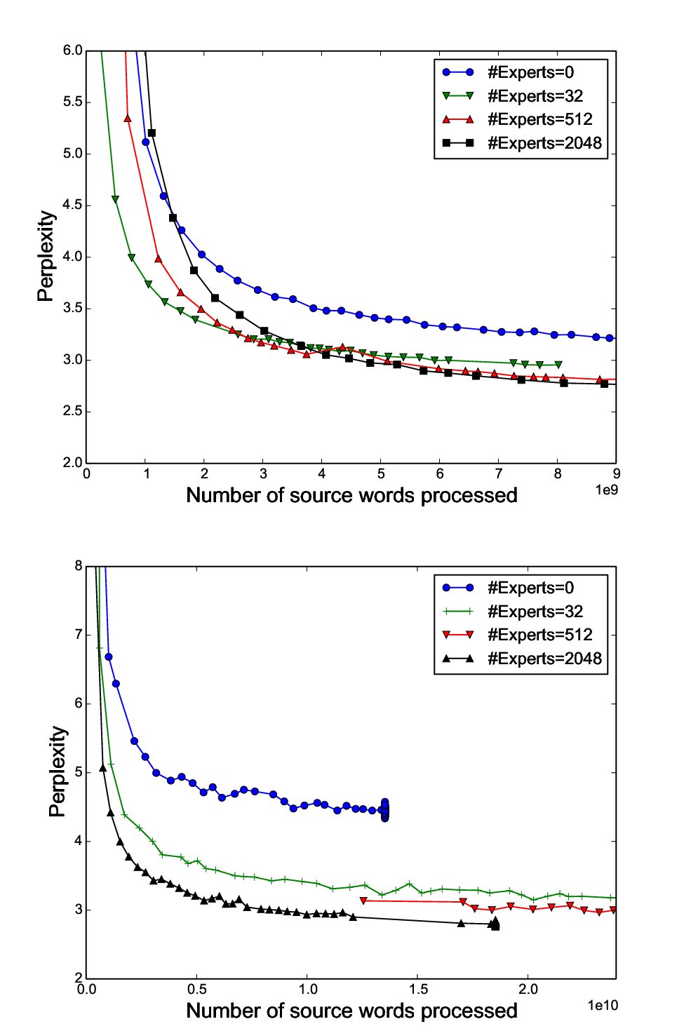
Figure 4: Perplexity on WMT’14 En$\rightarrow$ Fr (left) and Google Production En$\rightarrow$ Fr (right) datasets as a function of number of words processed. The large differences between models at the beginning of training are due to different batch sizes. All models incur the same computational budget (85M ops/timestep) except the one with no experts.

图 4：WMT’14 En$\rightarrow$ Fr（左）与 Google 生产 En$\rightarrow$ Fr（右）数据集上的困惑度随已处理词数的变化。训练开始时模型之间的较大差异来自不同的批次大小。除没有专家的那个模型外，所有模型的计算预算相同（每时间步 8500 万次运算）。

We found that the experts indeed become highly specialized by syntax and/or semantics, as can be seen in Table 9. For example, one expert is used when the indefinite article “a" introduces the direct object in a verb phrase indicating importance or leadership.

我们发现专家确实会按句法与/或语义高度专门化，如表 9 所示。例如，当不定冠词 “a” 在表示重要性或领导地位的动词短语中引入直接宾语时，会用到某一个专家。

Expert 381	Expert 752	Expert 2004
… with researchers , …	… plays a core …	… with rapidly growing …
… to innovation .	… plays a critical …	… under static conditions …
… tics researchers .	… provides a legislative …	… to swift ly …
… the generation of …	… play a leading …	… to dras tically …
… technology innovations is …	… assume a leadership …	… the rapid and …
… technological innovations , …	… plays a central …	… the fast est …
… support innovation throughout …	… taken a leading …	… the Quick Method …
… role innovation will …	… established a reconciliation …	… rec urrent ) …
… research scienti st …	… played a vital …	… provides quick access …
… promoting innovation where …	… have a central …	… of volatile organic …
…	…	…

Table 9: Contexts corresponding to a few of the 2048 experts in the MoE layer in the encoder portion of the WMT’14 En$\rightarrow$ Fr translation model. For each expert $i$, we sort the inputs in a training batch in decreasing order of $G(x)_{i}$, and show the words surrounding the corresponding positions in the input sentences.

Expert 381	Expert 752	Expert 2004
… with researchers , …	… plays a core …	… with rapidly growing …
… to innovation .	… plays a critical …	… under static conditions …
… tics researchers .	… provides a legislative …	… to swift ly …
… the generation of …	… play a leading …	… to dras tically …
… technology innovations is …	… assume a leadership …	… the rapid and …
… technological innovations , …	… plays a central …	… the fast est …
… support innovation throughout …	… taken a leading …	… the Quick Method …
… role innovation will …	… established a reconciliation …	… rec urrent ) …
… research scienti st …	… played a vital …	… provides quick access …
… promoting innovation where …	… have a central …	… of volatile organic …
…	…	…

表 9：WMT’14 En$\rightarrow$ Fr 翻译模型编码器部分 MoE 层中 2048 个专家里若干专家对应的上下文。对每个专家 $i$，我们按 $G(x)_{i}$ 降序对一个训练批次中的输入排序，并给出输入句子中相应位置周围的词。

F Strictly Balanced Gating

F 严格均衡门控

Due to some peculiarities in our infrastructure which have since been fixed, at the time we ran some of the machine translation experiments, our models ran faster if every expert received exactly the same batch size. To accommodate this, we used a different gating function which we describe below.

由于我们基础设施中一些后来已被修复的特殊性，在我们跑部分机器翻译实验时，如果每个专家收到恰好相同的批次大小，模型会跑得更快。为适应这一点，我们使用了下面描述的另一种门控函数。

Recall that we define the softmax gating function to be:

回顾一下，我们把 softmax 门控函数定义为：

$$G_{\sigma}(x)=Softmax(x\cdot W_{g}) \tag{15}$$

Sparse Gating (alternate formulation):

To obtain a sparse gating vector, we multiply $G_{\sigma}(x)$ component-wise with a sparse mask $M(G_{\sigma}(x))$ and normalize the output. The mask itself is a function of $G_{\sigma}(x)$ and specifies which experts are assigned to each input example:

稀疏门控（另一种写法）：

为得到稀疏的门控向量，我们把 $G_{\sigma}(x)$ 与稀疏掩码 $M(G_{\sigma}(x))$ 按分量相乘，并对输出归一化。掩码本身是 $G_{\sigma}(x)$ 的函数，指定每个输入样本被分配给哪些专家：

$$G(x)_{i}=\frac{G_{\sigma}(x)_{i}M(G_{\sigma}(x))_{i}}{\sum_{j=1}^{n}G_{\sigma}(x)_{j}M(G_{\sigma}(x))_{j}} \tag{16}$$

Top-K Mask:

To implement top-k gating in this formulation, we would let $M(v)=TopK(v,k)$, where:

Top-K 掩码：

要在这一写法中实现 top-k 门控，我们可以令 $M(v)=TopK(v,k)$，其中：

$TopK(v,k)_{i}=\begin{cases}1&\text{ifv_{i}$is in the top$k$elements of$v$.}\
0&\text{otherwise.}\end{cases} \tag{17}$$

Batchwise Mask:

To force each expert to receive the exact same number of examples, we introduce an alternative mask function, $M_{batchwise}(X,m)$, which operates over batches of input vectors. Instead of keeping the top $k$ values per example, we keep the top $m$ values per expert across the training batch, where $m=\frac{k|X|}{n}$, so that each example is sent to an average of $k$ experts.

批次掩码：

为迫使每个专家收到恰好相同数量的样本，我们引入另一种掩码函数 $M_{batchwise}(X,m)$，它在输入向量的批次上操作。我们不再对每个样本保留前 $k$ 个值，而是对每个专家在训练批次上保留前 $m$ 个值，其中 $m=\frac{k|X|}{n}$，从而使每个样本平均被送到 $k$ 个专家。

$M_{batchwise}(X,m)_{j,i}=\begin{cases}1&\text{ifX_{j,i}$is in the top$m$values for to expert$i$}\
0&\text{otherwise}\end{cases} \tag{18}$$

As our experiments suggest and also observed in  (Ioffe & Szegedy, 2015), using a batchwise function during training (such as $M_{batchwise}$) requires modifications to the inference when we may not have a large batch of examples. Our solution to this is to train a vector $T$ of per-expert threshold values to approximate the effects of the batchwise mask. We use the following mask at inference time:

如我们的实验所示，也如 Ioffe 与 Szegedy（2015）所观察到的，在训练时使用批次函数（如 $M_{batchwise}$）需要在推理时做修改，因为那时我们可能没有大批样本。我们的解决办法是训练一个每位专家阈值组成的向量 $T$，以近似批次掩码的效果。我们在推理时使用下面的掩码：

$M_{threshold}(x,T)_{i}=\begin{cases}1&\text{ifx_{i}>T_{i}$}\
0&\text{otherwise}\end{cases} \tag{19}$$

To learn the threshold values, we apply an additional loss at training time which is minimized when the batchwise mask and the threshold mask are identical.

为学习阈值，我们在训练时施加额外损失，当批次掩码与阈值掩码完全相同时该损失取最小。

$$L_{batchwise}(X,T,m)=\sum_{j=1}^{|X|}\sum_{i=1}^{n}(M_{threshold}(x,T)_{i}-M_{batchwise}(X,m)_{j,i})(X_{j,i}-T_{i}) \tag{20}$$

G Attention Function

G 注意力函数

The attention mechanism described in GNMT  (Wu et al., 2016) involves a learned “Attention Function" $A(x_{i},y_{j})$ which takes a “source vector" $x_{i}$ and a “target vector" $y_{j}$, and must be computed for every source time step $i$ and target time step $j$. In GNMT, the attention function is implemented as a feed forward neural network with a hidden layer of size $n$. It can be expressed as:

GNMT（Wu 等，2016）中描述的注意力机制涉及一个学得的“注意力函数” $A(x_{i},y_{j})$，它接收一个“源向量” $x_{i}$ 与一个“目标向量” $y_{j}$，并且必须对每个源时间步 $i$ 与目标时间步 $j$ 计算。在 GNMT 中，注意力函数实现为一个带大小为 $n$ 的隐藏层的前馈神经网络。它可以写成：

$$A_{GNMT}(x_{i},y_{j})=\sum_{d=1}^{n}V_{d}tanh((x_{i}U)_{d}+(y_{j}W)_{d}) \tag{21}$$

Where $U$ and $W$ are trainable weight matrices and $V$ is a trainable weight vector.

其中 $U$ 与 $W$ 是可训练的权重矩阵，$V$ 是可训练的权重向量。

For performance reasons, in our models, we used a slightly different attention function:

出于性能考虑，在我们的模型中，我们使用了略有不同的注意力函数：

$$A(x_{i},y_{j})=\sum_{d=1}^{n}V_{d}tanh((x_{i}U)_{d})tanh((y_{j}W)_{d}) \tag{22}$$

With our attention function, we can simultaneously compute the attention function on multiple source time steps and multiple target time steps using optimized matrix multiplications. We found little difference in quality between the two functions.

使用我们的注意力函数，我们可以用经过优化的矩阵乘法，同时在多个源时间步与多个目标时间步上计算注意力函数。我们发现这两个函数在质量上差别很小。