Spectral Normalization for Generative Adversarial Networks
Spectral Normalization for Generative Adversarial Networks
生成对抗网络的谱归一化
Takeru Miyato Toshiki Kataoka Masanori Koyama Yuichi Yoshida {miyato, kataoka}@preferred.jpkoyama.masanori@gmail.comyyoshida@nii.ac.jp Affiliation: Preferred Networks, Inc. Ritsumeikan University National Institute of Informatics
Abstract
摘要
One of the challenges in the study of generative adversarial networks is the instability of its training. In this paper, we propose a novel weight normalization technique called spectral normalization to stabilize the training of the discriminator. Our new normalization technique is computationally light and easy to incorporate into existing implementations. We tested the efficacy of spectral normalization on CIFAR10, STL-10, and ILSVRC2012 dataset, and we experimentally confirmed that spectrally normalized GANs (SN-GANs) is capable of generating images of better or equal quality relative to the previous training stabilization techniques. The code with Chainer Tokui et al. 2015, generated images and pretrained models are available at https://github.com/pfnet-research/sngan_projection.
生成对抗网络研究中的一大挑战是训练不稳定。本文提出一种称为谱归一化的新型权重归一化技术,用以稳定判别器的训练。该归一化计算轻量,易于并入已有实现。我们在 CIFAR10、STL-10 与 ILSVRC2012 上检验谱归一化的效力,实验确认谱归一化 GAN(SN-GANs)相对先前训练稳定技术,能够生成质量更好或相当的图像。基于 Chainer(Tokui et al. 2015)的代码、生成图像与预训练模型见 https://github.com/pfnet-research/sngan_projection。
1 Introduction
1 引言
Generative adversarial networks (GANs) Goodfellow et al. 2014 have been enjoying considerable success as a framework of generative models in recent years, and it has been applied to numerous types of tasks and datasets Radford et al. 2016; Salimans et al. 2016; Ho & Ermon 2016; Li et al. 2017. In a nutshell, GANs are a framework to produce a model distribution that mimics a given target distribution, and it consists of a generator that produces the model distribution and a discriminator that distinguishes the model distribution from the target. The concept is to consecutively train the model distribution and the discriminator in turn, with the goal of reducing the difference between the model distribution and the target distribution measured by the best discriminator possible at each step of the training. GANs have been drawing attention in the machine learning community not only for its ability to learn highly structured probability distribution but also for its theoretically interesting aspects. For example, Nowozin et al. 2016; Uehara et al. 2016; Mohamed & Lakshminarayanan 2017 revealed that the training of the discriminator amounts to the training of a good estimator for the density ratio between the model distribution and the target. This is a perspective that opens the door to the methods of implicit models Mohamed & Lakshminarayanan 2017; Tran et al. 2017 that can be used to carry out variational optimization without the direct knowledge of the density function.
生成对抗网络(GANs,Goodfellow et al. 2014)近年来作为生成模型框架取得可观成功,并被应用于众多任务与数据集(Radford et al. 2016;Salimans et al. 2016;Ho & Ermon 2016;Li et al. 2017)。简言之,GAN 旨在产生模仿给定目标分布的模型分布:生成器产生模型分布,判别器区分模型分布与目标。概念是轮流连续训练模型分布与判别器,目标是在训练每一步用当时尽可能好的判别器,缩小模型分布与目标分布之间由其度量的差异。GAN 引起机器学习社区关注,不仅因其能学习高度结构化的概率分布,也因其 在理论上也引人关注的方面。例如 Nowozin et al. 2016;Uehara et al. 2016;Mohamed & Lakshminarayanan 2017 指出,训练判别器等价于训练模型分布与目标之间密度比的良好估计器。这一视角通向 隐式模型 方法(Mohamed & Lakshminarayanan 2017;Tran et al. 2017),可在不直接知道密度函数的情况下做变分优化。
A persisting challenge in the training of GANs is the performance control of the discriminator. In high dimensional spaces, the density ratio estimation by the discriminator is often inaccurate and unstable during the training, and generator networks fail to learn the multimodal structure of the target distribution. Even worse, when the support of the model distribution and the support of the target distribution are disjoint, there exists a discriminator that can perfectly distinguish the model distribution from the target Arjovsky & Bottou 2017. Once such discriminator is produced in this situation, the training of the generator comes to complete stop, because the derivative of the so-produced discriminator with respect to the input turns out to be 0. This motivates us to introduce some form of restriction to the choice of the discriminator.
GAN 训练中持续存在的挑战是对判别器表现的控制。在高维空间中,判别器对密度比的估计在训练过程中往往不准确且不稳定,生成器网络难以学到目标分布的多峰结构。更糟的是,当模型分布的支撑与目标分布的支撑不相交时,存在能完美区分二者的判别器(Arjovsky & Bottou 2017)。一旦在此情形下得到这样的判别器,生成器训练就会完全停滞,因为该判别器对输入的导数为 0。这促使我们在判别器的选择上引入某种限制。
In this paper, we propose a novel weight normalization method called spectral normalization that can stabilize the training of discriminator networks. Our normalization enjoys following favorable properties.
本文提出一种称为 谱归一化 的新型权重归一化方法,可稳定判别器网络的训练。该归一化具有以下有利性质。
- • Lipschitz constant is the only hyper-parameter to be tuned, and the algorithm does not require intensive tuning of the only hyper-parameter for satisfactory performance.
- • Lipschitz 常数是唯一需调的超参数,算法不必对这唯一超参数做密集调优也能取得满意表现。
- • Implementation is simple and the additional computational cost is small.
- • 实现简单,额外计算开销小。
In fact, our normalization method also functioned well even without tuning Lipschitz constant, which is the only hyper parameter. In this study, we provide explanations of the effectiveness of spectral normalization for GANs against other regularization techniques, such as weight normalization Salimans & Kingma 2016, weight clipping Arjovsky et al. 2017, and gradient penalty Gulrajani et al. 2017. We also show that, in the absence of complimentary regularization techniques (e.g., batch normalization, weight decay and feature matching on the discriminator), spectral normalization can improve the sheer quality of the generated images better than weight normalization and gradient penalty.
事实上,即便不调 Lipschitz 常数(唯一超参数),我们的归一化方法也能良好工作。本研究解释谱归一化相对权重归一化(Salimans & Kingma 2016)、权重裁剪(Arjovsky et al. 2017)与梯度惩罚(Gulrajani et al. 2017)等其他正则技术对 GAN 的有效性。我们还表明:在没有配套正则(如判别器上的批归一化、权重衰减与特征匹配)时,谱归一化相对权重归一化与梯度惩罚,更能直接提升生成图像的质量。
2 Method
2 方法
In this section, we will lay the theoretical groundwork for our proposed method. Let us consider a simple discriminator made of a neural network of the following form, with the input :
本节为所提方法奠定理论框架。考虑如下形式的简单神经网络判别器,输入为 :
where is the learning parameters set, , , and is an element-wise non-linear activation function. We omit the bias term of each layer for simplicity. The final output of the discriminator is given by
其中 为学习参数集,,, 为逐元素非线性激活。为简洁省略各层偏置项。判别器最终输出为
where is an activation function corresponding to the divergence of distance measure of the user’s choice. The standard formulation of GANs is given by
其中 为对应用户所选散度或距离度量的激活函数。GAN 的标准表述为
where min and max of and are taken over the set of generator and discriminator functions, respectively. The conventional form of Goodfellow et al. 2014 is given by where is the data distribution and is the (model) generator distribution to be learned through the adversarial min-max optimization. The activation function that is used in the of this expression is some continuous function with range (e.g, sigmoid function). It is known that, for a fixed generator , the optimal discriminator for this form of is given by .
其中对 与 的 min 与 max 分别在生成器与判别器函数集合上取。 的常规形式(Goodfellow et al. 2014)为 ,其中 为数据分布, 为通过对抗 min-max 优化学习的(模型)生成器分布。该表达式中 所用的激活 是值域为 的某连续函数(例如 sigmoid)。已知对固定生成器 ,该形式 的最优判别器为 。
The machine learning community has been pointing out recently that the function space from which the discriminators are selected crucially affects the performance of GANs. A number of works Uehara et al. 2016; Qi 2017; Gulrajani et al. 2017 advocate the importance of Lipschitz continuity in assuring the boundedness of statistics. For example, the optimal discriminator of GANs on the above standard formulation takes the form
机器学习社区近来指出:选择判别器的函数空间对 GAN 表现至关重要。不少工作(Uehara et al. 2016;Qi 2017;Gulrajani et al. 2017)强调 Lipschitz 连续性对保证统计量有界的重要性。例如,上述标准表述下 GAN 的最优判别器取形式
and its derivative
其导数
can be unbounded or even incomputable. This prompts us to introduce some regularity condition to the derivative of .
可能无界甚至不可计算。这促使我们对 的导数引入某种正则性条件。
A particularly successful works in this array are Qi 2017; Arjovsky et al. 2017; Gulrajani et al. 2017, which proposed methods to control the Lipschitz constant of the discriminator by adding regularization terms defined on input examples . We would follow their footsteps and search for the discriminator from the set of -Lipschitz continuous functions, that is,
这一方向上较为成功的工作包括 Qi 2017;Arjovsky et al. 2017;Gulrajani et al. 2017:它们通过对输入样本 定义的正则项来控制判别器的 Lipschitz 常数。我们沿袭其思路,从 -Lipschitz 连续函数集合中搜索判别器 ,即
where we mean by the smallest value such that for any , with the norm being the norm.
其中 表示使对任意 有 的最小 ,范数为 范数。
While input based regularizations allow for relatively easy formulations based on samples, they also suffer from the fact that, they cannot impose regularization on the space outside of the supports of the generator and data distributions without introducing somewhat heuristic means. A method we would introduce in this paper, called spectral normalization, is a method that aims to skirt this issue by normalizing the weight matrices using the technique devised by Yoshida & Miyato 2017.
基于输入的正则相对容易用样本表述,但也有局限:若不引入某种启发式手段,就无法对生成器与数据分布支撑之外的空间施加正则。本文引入的 谱归一化 方法,旨在用 Yoshida & Miyato 2017 提出的技术对权重矩阵做 归一化,从而绕开该问题。
2.1 Spectral Normalization
2.1 谱归一化
Our spectral normalization controls the Lipschitz constant of the discriminator function by literally constraining the spectral norm of each layer . By definition, Lipschitz norm is equal to , where is the spectral norm of the matrix ( matrix norm of )
谱归一化通过约束每一层 的谱范数,来控制判别器函数 的 Lipschitz 常数。按定义,Lipschitz 范数 等于 ,其中 为矩阵 的谱范数( 的 矩阵范数)
which is equivalent to the largest singular value of . Therefore, for a linear layer , the norm is given by . If the Lipschitz norm of the activation function is equal to 1 [^1], we can use the inequality to observe the following bound on :
它等于 的最大奇异值。因此对线性层 ,范数为 。若激活函数的 Lipschitz 范数 等于 1[^1],则可利用不等式 ,得到 的如下上界:
Our spectral normalization normalizes the spectral norm of the weight matrix so that it satisfies the Lipschitz constraint :
我们的 谱归一化 对权重矩阵 做谱范数归一化,使其满足 Lipschitz 约束 :
If we normalize each using (8), we can appeal to the inequality (7) and the fact that to see that is bounded from above by .
若用 (8) 归一化每个 ,则可借助不等式 (7) 以及 ,看出 被 1 从上界定。
Here, we would like to emphasize the difference between our spectral normalization and spectral norm ”regularization” introduced by Yoshida & Miyato 2017. Unlike our method, spectral norm ”regularization” penalizes the spectral norm by adding explicit regularization term to the objective function. Their method is fundamentally different from our method in that they do not make an attempt to ‘set’ the spectral norm to a designated value. Moreover, when we reorganize the derivative of our normalized cost function and rewrite our objective function (12), we see that our method is augmenting the cost function with a sample data dependent regularization function. Spectral norm regularization, on the other hand, imposes sample data independent regularization on the cost function, just like L2 regularization and Lasso.
在此我们想强调本谱归一化与 Yoshida & Miyato 2017 引入的谱范数「正则」之间的差别。与我们的方法不同,谱范数「正则」通过在目标函数中加入显式正则项来惩罚谱范数。二者本质不同:他们并不试图把谱范数「设」为指定值。此外,当我们整理归一化代价函数的导数并改写目标(12)时,可见本方法是在代价函数上附加了依赖样本数据的正则函数;而谱范数正则则像 L2 正则与 Lasso 一样,对代价函数施加与样本无关的正则。
2.2 Fast Approximation of the Spectral Norm
2.2 谱范数 的快速近似
As we mentioned above, the spectral norm that we use to regularize each layer of the discriminator is the largest singular value of . If we naively apply singular value decomposition to compute the at each round of the algorithm, the algorithm can become computationally heavy. Instead, we can use the power iteration method to estimate Golub & Van der Vorst 2000; Yoshida & Miyato 2017. With power iteration method, we can estimate the spectral norm with very small additional computational time relative to the full computational cost of the vanilla GANs. Please see Appendix A for the detail method and Algorithm 1 for the summary of the actual spectral normalization algorithm.
如上所述,用来正则判别器各层的谱范数 即 的最大奇异值。若每轮都朴素做奇异值分解算 ,算法会计算沉重。相反,可用幂迭代估计 (Golub & Van der Vorst 2000;Yoshida & Miyato 2017)。相对原版 GAN 的总计算量,幂迭代估计谱范数的额外时间非常小。细节见附录 A,实际谱归一化算法总结见算法 1。
2.3 Gradient analysis of the spectrally normalized weights
2.3 谱归一化权重的梯度分析
The gradient[^2] of with respect to is:
对 的梯度[^2]为:
where is the matrix whose -th entry is and zero everywhere else, and and are respectively the first left and right singular vectors of . If is the hidden layer in the network to be transformed by , the derivative of the calculated over the mini-batch with respect to of the discriminator is given by:
其中 为 元为 1、其余为 0 的矩阵, 与 分别为 的第一左、右奇异向量。若 是网络中将被 变换的隐层,则在 mini-batch 上计算的 对判别器 的 的导数为:
where , , and represents empirical expectation over the mini-batch. when for some .
其中 ,, 表示 mini-batch 上的经验期望。当 (某 )时,。
We would like to comment on the implication of (12). The first term is the same as the derivative of the weights without normalization. In this light, the second term in the expression can be seen as the regularization term penalizing the first singular components with the adaptive regularization coefficient . is positive when and are pointing in similar direction, and this prevents the column space of from concentrating into one particular direction in the course of the training. In other words, spectral normalization prevents the transformation of each layer from becoming to sensitive in one direction. We can also use spectral normalization to devise a new parametrization for the model. Namely, we can split the layer map into two separate trainable components: spectrally normalized map and the spectral norm constant. As it turns out, this parametrization has its merit on its own and promotes the performance of GANs (See Appendix E).
我们想评论 (12) 的含义。第一项 与未归一化时权重的导数相同。由此,表达式中的第二项可视为以 自适应 正则系数 惩罚第一奇异分量的正则项。当 与 指向相近方向时 为正,这会阻止训练过程中 的列空间集中到某一特定方向。换言之,谱归一化防止各层变换对单一方向过于敏感。也可用谱归一化设计新的模型参数化:把层映射拆成谱归一化映射与谱范数常数两个可训练分量。事实证明该参数化本身有其价值,并能提升 GAN 表现(见附录 E)。
3 Spectral Normalization vs Other Regularization Techniques
3 谱归一化与其他正则技术
The weight normalization introduced by Salimans & Kingma 2016 is a method that normalizes the norm of each row vector in the weight matrix. Mathematically, this is equivalent to requiring the weight by the weight normalization :
Salimans & Kingma 2016 引入的权重归一化,是把权重矩阵每行向量的 范数归一化。数学上等价于要求权重归一化后的 满足:
where is a -th singular value of matrix . Therefore, up to a scaler, this is same as the Frobenius normalization, which requires the sum of the squared singular values to be 1. These normalizations, however, inadvertently impose much stronger constraint on the matrix than intended. If is the weight normalized matrix of dimension , the norm for a fixed unit vector is maximized at when and for , which means that is of rank one. Similar thing can be said to the Frobenius normalization (See the appendix for more details). Using such corresponds to using only one feature to discriminate the model probability distribution from the target. In order to retain as much norm of the input as possible and hence to make the discriminator more sensitive, one would hope to make the norm of large. For weight normalization, however, this comes at the cost of reducing the rank and hence the number of features to be used for the discriminator. Thus, there is a conflict of interests between weight normalization and our desire to use as many features as possible to distinguish the generator distribution from the target distribution. The former interest often reigns over the other in many cases, inadvertently diminishing the number of features to be used by the discriminators. Consequently, the algorithm would produce a rather arbitrary model distribution that matches the target distribution only at select few features. Weight clipping Arjovsky et al. 2017 also suffers from same pitfall.
其中 为矩阵 的第 个奇异值。因此至多差一个标量,这与要求平方奇异值之和为 1 的 Frobenius 归一化相同。然而这些归一化无意中对矩阵施加了比预期更强的约束。若 为 的权重归一化矩阵,则对固定单位向量 , 在 且 ()时取最大 ,这意味着 秩为一。Frobenius 归一化亦有类似结论(详见附录)。使用这样的 相当于只用一个特征来区分模型概率分布与目标。为尽可能保留输入范数、从而使判别器更敏感,人们希望 较大。但对权重归一化而言,这要以降低秩、从而减少判别可用特征数为代价。于是权重归一化与「尽量用多特征区分生成器分布与目标」的愿望发生冲突。前者常常压倒后者,无意中削弱判别器可用特征数。结果算法会产出相当任意的模型分布,只在少数选定特征上匹配目标。权重裁剪(Arjovsky et al. 2017)也落入同一陷阱。
Our spectral normalization, on the other hand, do not suffer from such a conflict in interest. Note that the Lipschitz constant of a linear operator is determined only by the maximum singular value. In other words, the spectral norm is independent of rank. Thus, unlike the weight normalization, our spectral normalization allows the parameter matrix to use as many features as possible while satisfying local -Lipschitz constraint. Our spectral normalization leaves more freedom in choosing the number of singular components (features) to feed to the next layer of the discriminator.
我们的谱归一化则不会陷入此类利益冲突。注意线性算子的 Lipschitz 常数只由最大奇异值决定;换言之,谱范数与秩无关。因此与权重归一化不同,谱归一化允许参数矩阵在满足局部 1-Lipschitz 约束的同时尽可能多用特征。谱归一化在选择送入判别器下一层的奇异分量(特征)数目上留下更多自由。
Brock et al. 2016 introduced orthonormal regularization on each weight to stabilize the training of GANs. In their work, Brock et al. 2016 augmented the adversarial objective function by adding the following term:
Brock et al. 2016 对每个权重引入正交归一正则以稳定 GAN 训练。他们在对抗目标上附加如下项:
While this seems to serve the same purpose as spectral normalization, orthonormal regularization are mathematically quite different from our spectral normalization because the orthonormal regularization destroys the information about the spectrum by setting all the singular values to one. On the other hand, spectral normalization only scales the spectrum so that the its maximum will be one.
这看似与谱归一化目的相同,但正交归一正则在数学上与谱归一化颇为不同:它把所有奇异值设为 1,从而破坏谱信息;而谱归一化只缩放谱,使最大奇异值为 1。
Gulrajani et al. 2017 used Gradient penalty method in combination with WGAN. In their work, they placed -Lipschitz constant on the discriminator by augmenting the objective function with the regularizer that rewards the function for having local 1-Lipschitz constant (i.e. ) at discrete sets of points of the form generated by interpolating a sample from generative distribution and a sample from the data distribution. While this rather straightforward approach does not suffer from the problems we mentioned above regarding the effective dimension of the feature space, the approach has an obvious weakness of being heavily dependent on the support of the current generative distribution. As a matter of course, the generative distribution and its support gradually changes in the course of the training, and this can destabilize the effect of such regularization. In fact, we empirically observed that a high learning rate can destabilize the performance of WGAN-GP. On the contrary, our spectral normalization regularizes the function the operator space, and the effect of the regularization is more stable with respect to the choice of the batch. Training with our spectral normalization does not easily destabilize with aggressive learning rate. Moreover, WGAN-GP requires more computational cost than our spectral normalization with single-step power iteration, because the computation of requires one whole round of forward and backward propagation. In the appendix section, we compare the computational cost of the two methods for the same number of updates.
Gulrajani et al. 2017 把梯度惩罚与 WGAN 结合:通过对形如 的离散点集(由生成分布样本 与数据样本 插值得到)奖励局部 1-Lipschitz 常数(即 ),在目标上附加正则,从而对判别器施加 -Lipschitz 常数。这一相当直接的做法不会遭受上文关于特征空间有效维的问题,但明显弱点是严重依赖当前生成分布的支撑。训练过程中生成分布及其支撑逐渐变化,可能使此类正则效果不稳定。事实上我们经验上观察到高学习率会使 WGAN-GP 表现不稳。相反,谱归一化在算子空间上正则函数,正则效果相对 batch 选择更稳定;用谱归一化训练时,激进学习率也不易破坏稳定。此外,相对单步幂迭代的谱归一化,WGAN-GP 计算更贵,因为计算 需要一整轮前向与反向。附录中我们按相同更新次数对比两种方法的计算开销。
4 Experiments
4 实验
In order to evaluate the efficacy of our approach and investigate the reason behind its efficacy, we conducted a set of extensive experiments of unsupervised image generation on CIFAR-10 Torralba et al. 2008 and STL-10 Coates et al. 2011, and compared our method against other normalization techniques. To see how our method fares against large dataset, we also applied our method on ILSVRC2012 dataset (ImageNet) Russakovsky et al. 2015 as well. This section is structured as follows. First, we will discuss the objective functions we used to train the architecture, and then we will describe the optimization settings we used in the experiments. We will then explain two performance measures on the images to evaluate the images produced by the trained generators. Finally, we will summarize our results on CIFAR-10, STL-10, and ImageNet.
为评估本方法效力并探究其背后原因,我们在 CIFAR-10(Torralba et al. 2008)与 STL-10(Coates et al. 2011)上做了大量无监督图像生成实验,并与其他归一化技术对比。为观察方法在大数据集上的表现,也在 ILSVRC2012(ImageNet,Russakovsky et al. 2015)上应用本方法。本节结构如下:先讨论训练所用目标函数,再描述优化设置;接着说明用于评估生成图像的两项性能度量;最后总结 CIFAR-10、STL-10 与 ImageNet 上的结果。
As for the architecture of the discriminator and generator, we used convolutional neural networks. Also, for the evaluation of the spectral norm for the convolutional weight , we treated the operator as a 2-D matrix of dimension [^3]. We trained the parameters of the generator with batch normalization Ioffe & Szegedy 2015. We refer the readers to Table 3 in the appendix section for more details of the architectures.
判别器与生成器结构均用卷积神经网络。对卷积权重 的谱范数,我们将其视为维数为 的二维矩阵[^3]。生成器参数用批归一化训练(Ioffe & Szegedy 2015)。结构细节见附录表 3。
For all methods other than WGAN-GP, we used the following standard objective function for the adversarial loss:
除 WGAN-GP 外,所有方法均使用如下标准对抗损失目标:
where is a latent variable, is the standard normal distribution , and is a deterministic generator function. We set to 128 for all of our experiments. For the updates of , we used the alternate cost proposed by Goodfellow et al. 2014 as used in Goodfellow et al. 2014 and Warde-Farley & Bengio 2017. For the updates of , we used the original cost defined in (15). We also tested the performance of the algorithm with the so-called hinge loss, which is given by
其中 为潜变量, 为标准正态 , 为确定性生成器。所有实验取 。更新 时使用 Goodfellow et al. 2014 提出的交替代价 ,亦见于 Warde-Farley & Bengio 2017。更新 时使用 (15) 中的原始代价。我们也用所谓 hinge 损失测试算法表现,形式为
respectively for the discriminator and the generator. Optimizing these objectives is equivalent to minimizing the so-called reverse KL divergence : . This type of loss has been already proposed and used in Lim & Ye 2017; Tran et al. 2017. The algorithm based on the hinge loss also showed good performance when evaluated with inception score and FID. For Wasserstein GANs with gradient penalty (WGAN-GP) Gulrajani et al. 2017, we used the following objective function: , where the regularization term is the one we introduced in the appendix section D.4.
分别对应判别器与生成器。优化这些目标等价于最小化所谓反向 KL 散度:。此类损失已由 Lim & Ye 2017;Tran et al. 2017 提出并使用。基于 hinge 损失的算法在 inception score 与 FID 评估下也表现良好。对带梯度惩罚的 Wasserstein GAN(WGAN-GP,Gulrajani et al. 2017),我们使用:,其中正则项即附录 D.4 所介绍者。
For quantitative assessment of generated examples, we used inception score Salimans et al. 2016 and Fréchet inception distance (FID) Heusel et al. 2017. Please see Appendix B.1 for the details of each score.
对生成样本的定量评估,我们使用 inception score(Salimans et al. 2016)与 Fréchet inception distance(FID,Heusel et al. 2017)。各项分数细节见附录 B.1。
4.1 Results on CIFAR10 and STL-10
4.1 CIFAR10 与 STL-10 上的结果
In this section, we report the accuracy of the spectral normalization (we use the abbreviation: SN-GAN for the spectrally normalized GANs) during the training, and the dependence of the algorithm’s performance on the hyperparmeters of the optimizer. We also compare the performance quality of the algorithm against those of other regularization/normalization techniques for the discriminator networks, including: Weight clipping Arjovsky et al. 2017, WGAN-GP Gulrajani et al. 2017, batch-normalization (BN) Ioffe & Szegedy 2015, layer normalization (LN) Ba et al. 2016, weight normalization (WN) Salimans & Kingma 2016 and orthonormal regularization (orthonormal) Brock et al. 2016. In order to evaluate the stand-alone efficacy of the gradient penalty, we also applied the gradient penalty term to the standard adversarial loss of GANs (15). We would refer to this method as ‘GAN-GP’. For weight clipping, we followed the original work Arjovsky et al. 2017 and set the clipping constant at 0.01 for the convolutional weight of each layer. For gradient penalty, we set to 10, as suggested in Gulrajani et al. 2017. For orthonormal, we initialized the each weight of with a randomly selected orthonormal operator and trained GANs with the objective function augmented with the regularization term used in Brock et al. 2016. For all comparative studies throughout, we excluded the multiplier parameter in the weight normalization method, as well as in batch normalization and layer normalization method. This was done in order to prevent the methods from overtly violating the Lipschitz condition. When we experimented with different multiplier parameter, we were in fact not able to achieve any improvement.
本节报告谱归一化(简称 SN-GAN)在训练中的准确度,以及算法表现对优化器超参数的依赖。我们也把算法表现质量与判别器网络上的其他正则/归一化技术对比,包括:权重裁剪(Arjovsky et al. 2017)、WGAN-GP(Gulrajani et al. 2017)、批归一化(BN,Ioffe & Szegedy 2015)、层归一化(LN,Ba et al. 2016)、权重归一化(WN,Salimans & Kingma 2016)以及正交归一正则(orthonormal,Brock et al. 2016)。为单独评估梯度惩罚效力,我们也把梯度惩罚项加到标准 GAN 对抗损失 (15) 上,称该方法为「GAN-GP」。权重裁剪按原作 Arjovsky et al. 2017,每层卷积权重裁剪常数 取 0.01。梯度惩罚按 Gulrajani et al. 2017 建议取 。对 orthonormal,我们用随机选取的正交算子初始化 的每个权重,并用 Brock et al. 2016 的正则项增强目标训练 GAN。所有对比实验中,我们排除权重归一化、批归一化与层归一化中的乘子参数 ,以防方法过度违反 Lipschitz 条件。当我们试验保留不同乘子参数时,实际上未能取得任何改进。
For optimization, we used the Adam optimizer Kingma & Ba 2015 in all of our experiments. We tested with 6 settings for (1) , the number of updates of the discriminator per one update of the generator and (2) learning rate and the first and second order momentum parameters (, ) of Adam. We list the details of these settings in Table 1 in the appendix section. Out of these 6 settings, A, B, and C are the settings used in previous representative works. The purpose of the settings D, E, and F is to the evaluate the performance of the algorithms implemented with more aggressive learning rates. For the details of the architectures of convolutional networks deployed in the generator and the discriminator, we refer the readers to Table 3 in the appendix section. The number of updates for GAN generator were 100K for all experiments, unless otherwise noted.
优化一律使用 Adam(Kingma & Ba 2015)。我们测试了 6 组设置,涉及 (1) (生成器每更新一次时判别器更新次数)与 (2) 学习率 以及 Adam 的一、二阶动量(,)。细节列于附录表 1。其中 A、B、C 为先前代表性工作所用设置;D、E、F 用于评估更激进学习率下的算法表现。生成器与判别器所用卷积网络结构见附录表 3。除非另注,GAN 生成器更新次数均为 100K。
| Setting | ||||
|---|---|---|---|---|
| A | 0.0001 | 0.5 | 0.9 | 5 |
| B | 0.0001 | 0.5 | 0.999 | 1 |
| C | 0.0002 | 0.5 | 0.999 | 1 |
| D | 0.001 | 0.5 | 0.9 | 5 |
| E | 0.001 | 0.5 | 0.999 | 5 |
| F | 0.001 | 0.9 | 0.999 | 5 |
Table 1: Hyper-parameter settings we tested in our experiments. , and are the hyperparameter settings following Gulrajani et al. 2017, Warde-Farley & Bengio 2017 and Radford et al. 2016, respectively.
| Setting | ||||
|---|---|---|---|---|
| A | 0.0001 | 0.5 | 0.9 | 5 |
| B | 0.0001 | 0.5 | 0.999 | 1 |
| C | 0.0002 | 0.5 | 0.999 | 1 |
| D | 0.001 | 0.5 | 0.9 | 5 |
| E | 0.001 | 0.5 | 0.999 | 5 |
| F | 0.001 | 0.9 | 0.999 | 5 |
表 1:实验中测试的超参数设置。、 与 分别沿用 Gulrajani et al. 2017、Warde-Farley & Bengio 2017 与 Radford et al. 2016 的超参数。
Firstly, we inspected the spectral norm of each layer during the training to make sure that our spectral normalization procedure is indeed serving its purpose. As we can see in the Figure 9 in the C.1, the spectral norms of these layers floats around – region throughout the training. Please see Appendix C.1 for more details.
首先,我们检查训练过程中各层谱范数,以确认谱归一化程序确实在起作用。如附录 C.1 图 9 所示,这些层的谱范数在训练全程浮动于约 –。更多细节见附录 C.1。
In Figures 1 and 2 we show the inception scores of each method with the settings A–F. We can see that spectral normalization is relatively robust with aggressive learning rates and momentum parameters. WGAN-GP fails to train good GANs at high learning rates and high momentum parameters on both CIFAR-10 and STL-10. Orthonormal regularization performed poorly for the setting E on the STL-10, but performed slightly better than our method with the optimal setting. These results suggests that our method is more robust than other methods with respect to the change in the setting of the training. Also, the optimal performance of weight normalization was inferior to both WGAN-GP and spectral normalization on STL-10, which consists of more diverse examples than CIFAR-10. Best scores of spectral normalization are better than almost all other methods on both CIFAR-10 and STL-10.
图 1 与图 2 展示各方法在设置 A–F 下的 inception score。可见谱归一化对激进学习率与动量参数相对稳健。WGAN-GP 在 CIFAR-10 与 STL-10 上均未能在高学习率与高动量下训出好的 GAN。正交归一正则在 STL-10 的设置 E 上表现较差,但在最优设置下略优于本方法。这些结果表明:相对其他方法,本方法对训练设置变化更稳健。此外,权重归一化的最优表现在比 CIFAR-10 样本更多样的 STL-10 上弱于 WGAN-GP 与谱归一化。谱归一化的最佳分数在 CIFAR-10 与 STL-10 上几乎都优于其他方法。
(a) CIFAR-10
(a) CIFAR-10
In Tables 2, we show the inception scores of the different methods with optimal settings on CIFAR-10 and STL-10 dataset. We see that SN-GANs performed better than almost all contemporaries on the optimal settings. SN-GANs performed even better with hinge loss (17).[^4]. For the training with same number of iterations, SN-GANs fell behind orthonormal regularization for STL-10. For more detailed comparison between orthonormal regularization and spectral normalization, please see section 4.1.2.
表 2 给出不同方法在 CIFAR-10 与 STL-10 上最优设置下的 inception score。可见 SN-GANs 在最优设置下几乎优于所有同期方法;使用 hinge 损失 (17) 时表现更好[^4]。在相同迭代次数下,SN-GANs 在 STL-10 上落后于正交归一正则。更细致的对比见 4.1.2 节。
| Method | Inception score | FID | ||
|---|---|---|---|---|
| CIFAR-10 | STL-10 | CIFAR-10 | STL-10 | |
| Real data | 11.24.12 | 26.08.26 | 7.8 | 7.9 |
| -Standard CNN- | ||||
| Weight clipping | 6.41.11 | 7.57.10 | 42.6 | 64.2 |
| GAN-GP | 6.93.08 | 37.7 | ||
| WGAN-GP | 6.68.06 | 8.42.13 | 40.2 | 55.1 |
| Batch Norm. | 6.27.10 | 56.3 | ||
| Layer Norm. | 7.19.12 | 7.61.12 | 33.9 | 75.6 |
| Weight Norm. | 6.84.07 | 7.16.10 | 34.7 | 73.4 |
| Orthonormal | 7.40.12 | 8.56.07 | 29.0 | 46.7 |
| (ours) SN-GANs | 7.42.08 | 8.28.09 | 29.3 | 53.1 |
| Orthonormal (2x updates) | 8.67.08 | 44.2 | ||
| (ours) SN-GANs (2x updates) | 8.69.09 | 47.5 | ||
| (ours) SN-GANs, Eq.(17) | 7.58.12 | 25.5 | ||
| (ours) SN-GANs, Eq.(17) (2x updates) | 8.79.14 | 43.2 | ||
| -ResNet-[^5] | ||||
| Orthonormal, Eq.(17) | 7.92.04 | 8.72.06 | 23.8.58 | 42.4.99 |
| (ours) SN-GANs, Eq.(17) | 8.22.05 | 9.10.04 | 21.7.21 | 40.1.50 |
| DCGAN | 6.64.14 | 7.84.07 | ||
| LR-GANs | 7.17.07 | |||
| Warde-Farley et al. | 7.72.13 | 8.51.13 | ||
| WGAN-GP (ResNet) | 7.86.08 |
Table 2: Inception scores and FIDs with unsupervised image generation on CIFAR-10. Radford et al. 2016 (experimented by Yang et al. 2017), Yang et al. 2017, Warde-Farley & Bengio 2017, Gulrajani et al. 2017
| Method | Inception score | FID | ||
|---|---|---|---|---|
| CIFAR-10 | STL-10 | CIFAR-10 | STL-10 | |
| Real data | 11.24.12 | 26.08.26 | 7.8 | 7.9 |
| -Standard CNN- | ||||
| Weight clipping | 6.41.11 | 7.57.10 | 42.6 | 64.2 |
| GAN-GP | 6.93.08 | 37.7 | ||
| WGAN-GP | 6.68.06 | 8.42.13 | 40.2 | 55.1 |
| Batch Norm. | 6.27.10 | 56.3 | ||
| Layer Norm. | 7.19.12 | 7.61.12 | 33.9 | 75.6 |
| Weight Norm. | 6.84.07 | 7.16.10 | 34.7 | 73.4 |
| Orthonormal | 7.40.12 | 8.56.07 | 29.0 | 46.7 |
| (ours) SN-GANs | 7.42.08 | 8.28.09 | 29.3 | 53.1 |
| Orthonormal (2x updates) | 8.67.08 | 44.2 | ||
| (ours) SN-GANs (2x updates) | 8.69.09 | 47.5 | ||
| (ours) SN-GANs, Eq.(17) | 7.58.12 | 25.5 | ||
| (ours) SN-GANs, Eq.(17) (2x updates) | 8.79.14 | 43.2 | ||
| -ResNet-[^5] | ||||
| Orthonormal, Eq.(17) | 7.92.04 | 8.72.06 | 23.8.58 | 42.4.99 |
| (ours) SN-GANs, Eq.(17) | 8.22.05 | 9.10.04 | 21.7.21 | 40.1.50 |
| DCGAN | 6.64.14 | 7.84.07 | ||
| LR-GANs | 7.17.07 | |||
| Warde-Farley et al. | 7.72.13 | 8.51.13 | ||
| WGAN-GP (ResNet) | 7.86.08 |
表 2:CIFAR-10 无监督图像生成的 inception score 与 FID。 Radford et al. 2016(由 Yang et al. 2017 实验), Yang et al. 2017, Warde-Farley & Bengio 2017, Gulrajani et al. 2017。
In Figure 6 we show the images produced by the generators trained with WGAN-GP, weight normalization, and spectral normalization. SN-GANs were consistently better than GANs with weight normalization in terms of the quality of generated images. To be more precise, as we mentioned in Section 3, the set of images generated by spectral normalization was clearer and more diverse than the images produced by the weight normalization. We can also see that WGAN-GP failed to train good GANs with high learning rates and high momentums (D,E and F). The generated images with GAN-GP, batch normalization, and layer normalization is shown in Figure 12 in the appendix section.
图 6 展示用 WGAN-GP、权重归一化与谱归一化训练的生成器所产图像。就生成图像质量而言,SN-GANs 始终优于带权重归一化的 GAN。更精确地说,如第 3 节所述,谱归一化生成的图像集合比权重归一化更清晰、更多样。也可看到 WGAN-GP 在高学习率与高动量(D、E、F)下未能训出好的 GAN。GAN-GP、批归一化与层归一化生成的图像见附录图 12。
We also compared our algorithm against multiple benchmark methods ans summarized the results on the bottom half of the Table 2. We also tested the performance of our method on ResNet based GANs used in Gulrajani et al. 2017. Please note that all methods listed thereof are all different in both optimization methods and the architecture of the model. Please see Table 8 and 5 in the appendix section for the detail network architectures. Our implementation of our algorithm was able to perform better than almost all the predecessors in the performance.
我们还与多种基准方法对比,结果总结于表 2 下半部。我们也在 Gulrajani et al. 2017 所用的基于 ResNet 的 GAN 上测试本方法。请注意其中所列方法在优化方法与模型结构上均有不同。网络结构细节见附录表 8 与表 5。我们的实现几乎优于所有先前工作。
4.1.1 Analysis of SN-GANs
(a) CIFAR-10
4.1.1 对 SN-GANs 的分析
(a) CIFAR-10
Singular values analysis on the weights of the discriminator
In Figure 3, we show the squared singular values of the weight matrices in the final discriminator produced by each method using the parameter that yielded the best inception score. As we predicted in Section 3, the singular values of the first to fifth layers trained with weight clipping and weight normalization concentrate on a few components. That is, the weight matrices of these layers tend to be rank deficit. On the other hand, the singular values of the weight matrices in those layers trained with spectral normalization is more broadly distributed. When the goal is to distinguish a pair of probability distributions on the low-dimensional nonlinear data manifold embedded in a high dimensional space, rank deficiencies in lower layers can be especially fatal. Outputs of lower layers have gone through only a few sets of rectified linear transformations, which means that they tend to lie on the space that is linear in most parts. Marginalizing out many features of the input distribution in such space can result in oversimplified discriminator. We can actually confirm the effect of this phenomenon on the generated images especially in Figure 6(b). The images generated with spectral normalization is more diverse and complex than those generated with weight normalization.
判别器 权重上的奇异值分析
图 3 展示各方法用取得最佳 inception score 的参数训出的最终判别器 中,权重矩阵的平方奇异值。如第 3 节所预测,权重裁剪与权重归一化训练的第一到第五层奇异值集中在少数分量上,即这些层的权重矩阵趋于秩亏。相反,谱归一化训练的这些层奇异值分布更广。当目标是区分嵌入在高维空间中低维非线性数据流形上的一对概率分布时,较低层的秩亏尤其致命。较低层输出只经过少数几组修正线性变换,因而大多落在局部近似线性的空间;在此空间中边缘化掉输入分布的许多特征,会导致过度简化的判别器。我们可在图 6(b) 等生成图像上实际确认该现象的影响:谱归一化生成的图像比权重归一化更多样、更复杂。
Training time
On CIFAR-10, SN-GANs is slightly slower than weight normalization (about 110 120% computational time), but significantly faster than WGAN-GP. As we mentioned in Section 3, WGAN-GP is slower than other methods because WGAN-GP needs to calculate the gradient of gradient norm . For STL-10, the computational time of SN-GANs is almost the same as vanilla GANs, because the relative computational cost of the power iteration (18) is negligible when compared to the cost of forward and backward propagation on CIFAR-10 (images size of STL-10 is larger ()). Please see Figure 10 in the appendix section for the actual computational time.
训练时间
在 CIFAR-10 上,SN-GANs 略慢于权重归一化(约 110~120% 计算时间),但显著快于 WGAN-GP。如第 3 节所述,WGAN-GP 更慢是因为需要计算梯度范数 的梯度。对 STL-10,SN-GANs 的计算时间几乎与原版 GAN 相同,因为相对 CIFAR-10 上前向与反向的开销,幂迭代 (18) 的相对成本可忽略(STL-10 图像更大,)。实际计算时间见附录图 10。
4.1.2 Comparison between SN-GANs and orthonormal regularization
Figure 4: The effect on the performance on STL-10 induced by the change of the feature map dimension of the final layer. The width of the highlighted region represents standard deviation of the results over multiple seeds of weight initialization. The orthonormal regularization does not perform well with large feature map dimension, possibly because of its design that forces the discriminator to use all dimensions including the ones that are unnecessary. For the setting of the optimizers’ hyper-parameters, We used the setting C, which was optimal for “orthonormal regularization”
4.1.2 SN-GANs 与正交归一正则的对比
图 4:改变最后一层特征图维数对 STL-10 表现的影响。高亮区域宽度表示多种权重初始化种子下结果的标准差。正交归一正则 在大特征图维数下表现不佳,可能因其设计迫使判别器使用所有维,包括不必要的维。优化器超参数我们使用对「正交归一正则」最优的设置 C。
In order to highlight the difference between our spectral normalization and orthonormal regularization, we conducted an additional set of experiments. As we explained in Section 3, orthonormal regularization is different from our method in that it destroys the spectral information and puts equal emphasis on all feature dimensions, including the ones that ’shall’ be weeded out in the training process. To see the extent of its possibly detrimental effect, we experimented by increasing the dimension of the feature space [^6], especially at the final layer (7th conv) for which the training with our spectral normalization prefers relatively small feature space (dimension ; see Figure 3(b)). As for the setting of the training, we selected the parameters for which the orthonormal regularization performed optimally. The figure 4 shows the result of our experiments. As we predicted, the performance of the orthonormal regularization deteriorates as we increase the dimension of the feature maps at the final layer. Our SN-GANs, on the other hand, does not falter with this modification of the architecture. Thus, at least in this perspective, we may such that our method is more robust with respect to the change of the network architecture.
为突出谱归一化与正交归一正则的差别,我们做了额外实验。如第 3 节所释,正交归一正则与本方法不同之处在于它破坏谱信息,并对所有特征维一视同仁——包括训练过程中「应当」被淘汰的维。为观察其可能的有害程度,我们增大特征空间维数[^6],尤其是最后一层(第 7 个卷积),而谱归一化训练偏好相对较小的特征空间(维数 ;见图 3(b))。训练设置选取正交归一正则表现最优的参数。图 4 给出实验结果。如所预测,随最后一层特征图维数增大,正交归一正则表现变差;而 SN-GANs 不因这一结构修改而动摇。至少从这一角度看,可以说本方法对网络结构变化更稳健。
4.2 Image Generation on ImageNet
4.2 ImageNet 上的图像生成
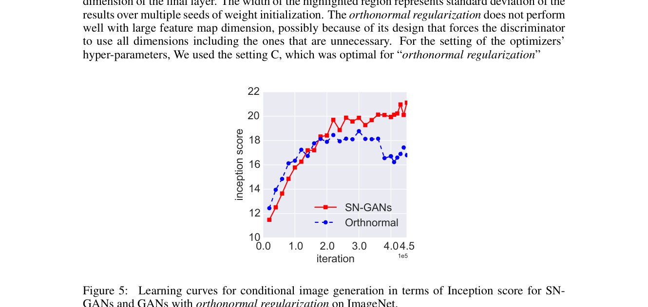
Figure 5: Learning curves for conditional image generation in terms of Inception score for SN-GANs and GANs with orthonormal regularization on ImageNet.
图 5:ImageNet 上条件图像生成的学习曲线(以 Inception score 计),对比 SN-GANs 与带 正交归一正则 的 GAN。
To show that our method remains effective on a large high dimensional dataset, we also applied our method to the training of conditional GANs on ILRSVRC2012 dataset with 1000 classes, each consisting of approximately 1300 images, which we compressed to pixels. Regarding the adversarial loss for conditional GANs, we used practically the same formulation used in Mirza & Osindero 2014, except that we replaced the standard GANs loss with hinge loss (17). Please see Appendix B.3 for the details of experimental settings.
为表明本方法在大型高维数据集上仍然有效,我们还把方法用于 ILSVRC2012 上的条件 GAN 训练:1000 类,每类约 1300 张图,压缩到 像素。条件 GAN 的对抗损失实际沿用 Mirza & Osindero 2014 的表述,只是把标准 GAN 损失换成 hinge 损失 (17)。实验设置细节见附录 B.3。
GANs without normalization and GANs with layer normalization collapsed in the beginning of training and failed to produce any meaningful images. GANs with orthonormal normalization Brock et al. 2016 and our spectral normalization, on the other hand, was able to produce images. The inception score of the orthonormal normalization however plateaued around 20Kth iterations, while SN kept improving even afterward (Figure 5.) To our knowledge, our research is the first of its kind in succeeding to produce decent images from ImageNet dataset with a single pair of a discriminator and a generator (Figure 7). To measure the degree of mode-collapse, we followed the footstep of Odena et al. 2017 and computed the intra MS-SSIM Odena et al. 2017 for pairs of independently generated GANs images of each class. We see that our SN-GANs ((intra MS-SSIM)=0.101) is suffering less from the mode-collapse than AC-GANs ((intra MS-SSIM)0.25).
无归一化的 GAN 与带层归一化的 GAN 在训练初期即崩溃,未能产生任何有意义图像。带正交归一(Brock et al. 2016)与我们的谱归一化的 GAN 则能产生图像。正交归一的 inception score 约在第 20K 次迭代后平台化,而 SN 之后仍继续提升(图 5)。据我们所知,本研究是首次用 单对 判别器与生成器从 ImageNet 数据集成功生成像样图像(图 7)。为度量模式崩溃程度,我们沿 Odena et al. 2017,对每类独立生成的 GAN 图像对计算 intra MS-SSIM(Odena et al. 2017)。可见 SN-GANs(intra MS-SSIM=0.101)比 AC-GANs(intra MS-SSIM0.25)更少受模式崩溃困扰。
To ensure that the superiority of our method is not limited within our specific setting, we also compared the performance of SN-GANs against orthonormal regularization on conditional GANs with projection discriminator Miyato & Koyama 2018 as well as the standard (unconditional) GANs. In our experiments, SN-GANs achieved better performance than orthonormal regularization for the both settings (See Figure 15 in the appendix section).
为确认本方法优势不限于特定设定,我们还在带 投影判别器(Miyato & Koyama 2018)的条件 GAN 以及标准(无条件)GAN 上,对比 SN-GANs 与 正交归一正则。实验中两种设定下 SN-GANs 均优于 正交归一正则(见附录图 15)。
5 Conclusion
5 结论
This paper proposes spectral normalization as a stabilizer of training of GANs. When we apply spectral normalization to the GANs on image generation tasks, the generated examples are more diverse than the conventional weight normalization and achieve better or comparative inception scores relative to previous studies. The method imposes global regularization on the discriminator as opposed to local regularization introduced by WGAN-GP, and can possibly used in combinations. In the future work, we would like to further investigate where our methods stand amongst other methods on more theoretical basis, and experiment our algorithm on larger and more complex datasets.
本文提出谱归一化作为 GAN 训练的稳定器。将谱归一化用于图像生成任务时,生成样本比传统权重归一化更多样,并相对先前研究取得更好或相当的 inception score。该方法对判别器施加全局正则,相对 WGAN-GP 引入的局部正则,并可能与之组合使用。未来工作中,我们希望在更理论的基础上进一步考察本方法相对其他方法的位置,并在更大、更复杂的数据集上实验本算法。
Acknowledgments
We would like to thank the members of Preferred Networks, Inc., particularly Shin-ichi Maeda, Eiichi Matsumoto, Masaki Watanabe and Keisuke Yahata for insightful comments and discussions. We also would like to thank anonymous reviewers and commenters on the OpenReview forum for insightful discussions.
致谢
感谢 Preferred Networks, Inc. 的成员,尤其是 Shin-ichi Maeda、Eiichi Matsumoto、Masaki Watanabe 与 Keisuke Yahata 的深刻评论与讨论。也感谢 OpenReview 论坛上的匿名审稿人与评论者的深入讨论。
References
参考文献
(a) CIFAR-10
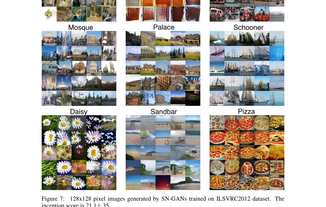
Figure 7: 128x128 pixel images generated by SN-GANs trained on ILSVRC2012 dataset. The inception score is 21.1.35.
图 7:在 ILSVRC2012 上训练的 SN-GANs 生成的 128×128 像素图像。inception score 为 21.1.35。
Arjovsky & Bottou (2017) Martin Arjovsky and Léon Bottou. Towards principled methods for training generative adversarial networks. In ICLR , 2017.
Arjovsky et al. (2017) Martin Arjovsky, Soumith Chintala, and Léon Bottou. Wasserstein generative adversarial networks. In ICML , pp. 214–223, 2017.
Arpit et al. (2016) Devansh Arpit, Yingbo Zhou, Bhargava U Kota, and Venu Govindaraju. Normalization propagation: A parametric technique for removing internal covariate shift in deep networks. In ICML , pp. 1168–1176, 2016.
Ba et al. (2016) Jimmy Lei Ba, Jamie Ryan Kiros, and Geoffrey E Hinton. Layer normalization. arXiv preprint arXiv:1607.06450 , 2016.
Brock et al. (2016) Andrew Brock, Theodore Lim, James M Ritchie, and Nick Weston. Neural photo editing with introspective adversarial networks. arXiv preprint arXiv:1609.07093 , 2016.
Coates et al. (2011) Adam Coates, Andrew Ng, and Honglak Lee. An analysis of single-layer networks in unsupervised feature learning. In AISTATS , pp. 215–223, 2011.
de Vries et al. (2017) Harm de Vries, Florian Strub, Jérémie Mary, Hugo Larochelle, Olivier Pietquin, and Aaron C Courville. Modulating early visual processing by language. In NIPS , pp. 6576–6586, 2017.
Dowson & Landau (1982) DC Dowson and BV Landau. The fréchet distance between multivariate normal distributions. Journal of Multivariate Analysis , 12(3):450–455, 1982.
Dumoulin et al. (2017) Vincent Dumoulin, Jonathon Shlens, and Manjunath Kudlur. A learned representation for artistic style. In ICLR , 2017.
Glorot et al. (2011) Xavier Glorot, Antoine Bordes, and Yoshua Bengio. Deep sparse rectifier neural networks. In AISTATS , pp. 315–323, 2011.
Golub & Van der Vorst (2000) Gene H Golub and Henk A Van der Vorst. Eigenvalue computation in the 20th century. Journal of Computational and Applied Mathematics , 123(1):35–65, 2000.
Goodfellow et al. (2014) Ian Goodfellow, Jean Pouget-Abadie, Mehdi Mirza, Bing Xu, David Warde-Farley, Sherjil Ozair, Aaron Courville, and Yoshua Bengio. Generative adversarial nets. In NIPS , pp. 2672–2680, 2014.
Gulrajani et al. (2017) Ishaan Gulrajani, Faruk Ahmed, Martin Arjovsky, Vincent Dumoulin, and Aaron Courville. Improved training of wasserstein GANs. arXiv preprint arXiv:1704.00028 , 2017.
He et al. (2016) Kaiming He, Xiangyu Zhang, Shaoqing Ren, and Jian Sun. Deep residual learning for image recognition. In CVPR , pp. 770–778, 2016.
Heusel et al. (2017) Martin Heusel, Hubert Ramsauer, Thomas Unterthiner, Bernhard Nessler, Günter Klambauer, and Sepp Hochreiter. GANs trained by a two time-scale update rule converge to a nash equilibrium. arXiv preprint arXiv:1706.08500 , 2017.
Ho & Ermon (2016) Jonathan Ho and Stefano Ermon. Generative adversarial imitation learning. In NIPS , pp. 4565–4573, 2016.
Ioffe & Szegedy (2015) Sergey Ioffe and Christian Szegedy. Batch normalization: Accelerating deep network training by reducing internal covariate shift. In ICML , pp. 448–456, 2015.
Jarrett et al. (2009) Kevin Jarrett, Koray Kavukcuoglu, Marc’Aurelio Ranzato, and Yann LeCun. What is the best multi-stage architecture for object recognition? In ICCV , pp. 2146–2153, 2009.
Jia et al. (2017) Kui Jia, Dacheng Tao, Shenghua Gao, and Xiangmin Xu. Improving training of deep neural networks via singular value bounding. In CVPR , 2017.
Kingma & Ba (2015) Diederik Kingma and Jimmy Ba. Adam: A method for stochastic optimization. In ICLR , 2015.
Li et al. (2017) Jiwei Li, Will Monroe, Tianlin Shi, Alan Ritter, and Dan Jurafsky. Adversarial learning for neural dialogue generation. In EMNLP , pp. 2147–2159, 2017.
Lim & Ye (2017) Jae Hyun Lim and Jong Chul Ye. Geometric GAN. arXiv preprint arXiv:1705.02894 , 2017.
Maas et al. (2013) Andrew L Maas, Awni Y Hannun, and Andrew Y Ng. Rectifier nonlinearities improve neural network acoustic models. In ICML Workshop on Deep Learning for Audio, Speech and Language Processing , 2013.
Mirza & Osindero (2014) Mehdi Mirza and Simon Osindero. Conditional generative adversarial nets. arXiv preprint arXiv:1411.1784 , 2014.
Miyato & Koyama (2018) Takeru Miyato and Masanori Koyama. cGANs with projection discriminator. In ICLR , 2018.
Mohamed & Lakshminarayanan (2017) Shakir Mohamed and Balaji Lakshminarayanan. Learning in implicit generative models. NIPS Workshop on Adversarial Training , 2017.
Nair & Hinton (2010) Vinod Nair and Geoffrey E Hinton. Rectified linear units improve restricted boltzmann machines. In ICML , pp. 807–814, 2010.
Nowozin et al. (2016) Sebastian Nowozin, Botond Cseke, and Ryota Tomioka. f-GAN: Training generative neural samplers using variational divergence minimization. In NIPS , pp. 271–279, 2016.
Odena et al. (2017) Augustus Odena, Christopher Olah, and Jonathon Shlens. Conditional image synthesis with auxiliary classifier GANs. In ICML , pp. 2642–2651, 2017.
Qi (2017) Guo-Jun Qi. Loss-sensitive generative adversarial networks on lipschitz densities. arXiv preprint arXiv:1701.06264 , 2017.
Radford et al. (2016) Alec Radford, Luke Metz, and Soumith Chintala. Unsupervised representation learning with deep convolutional generative adversarial networks. In ICLR , 2016.
Russakovsky et al. (2015) Olga Russakovsky, Jia Deng, Hao Su, Jonathan Krause, Sanjeev Satheesh, Sean Ma, Zhiheng Huang, Andrej Karpathy, Aditya Khosla, Michael Bernstein, Alexander C. Berg, and Li Fei-Fei. Imagenet large scale visual recognition challenge. International Journal of Computer Vision , 115(3):211–252, 2015.
Saito et al. (2017) Masaki Saito, Eiichi Matsumoto, and Shunta Saito. Temporal generative adversarial nets with singular value clipping. In ICCV , 2017.
Salimans & Kingma (2016) Tim Salimans and Diederik P Kingma. Weight normalization: A simple reparameterization to accelerate training of deep neural networks. In NIPS , pp. 901–909, 2016.
Salimans et al. (2016) Tim Salimans, Ian Goodfellow, Wojciech Zaremba, Vicki Cheung, Alec Radford, and Xi Chen. Improved techniques for training GANs. In NIPS , pp. 2226–2234, 2016.
Szegedy et al. (2015) Christian Szegedy, Wei Liu, Yangqing Jia, Pierre Sermanet, Scott Reed, Dragomir Anguelov, Dumitru Erhan, Vincent Vanhoucke, and Andrew Rabinovich. Going deeper with convolutions. In CVPR , pp. 1–9, 2015.
Tokui et al. (2015) Seiya Tokui, Kenta Oono, Shohei Hido, and Justin Clayton. Chainer: a next-generation open source framework for deep learning. In Proceedings of workshop on machine learning systems (LearningSys) in the twenty-ninth annual conference on neural information processing systems (NIPS) , 2015.
Torralba et al. (2008) Antonio Torralba, Rob Fergus, and William T Freeman. 80 million tiny images: A large data set for nonparametric object and scene recognition. IEEE Transactions on Pattern Analysis and Machine Intelligence , 30(11):1958–1970, 2008.
Tran et al. (2017) Dustin Tran, Rajesh Ranganath, and David M Blei. Deep and hierarchical implicit models. arXiv preprint arXiv:1702.08896 , 2017.
Uehara et al. (2016) Masatoshi Uehara, Issei Sato, Masahiro Suzuki, Kotaro Nakayama, and Yutaka Matsuo. Generative adversarial nets from a density ratio estimation perspective. NIPS Workshop on Adversarial Training , 2016.
Warde-Farley & Bengio (2017) David Warde-Farley and Yoshua Bengio. Improving generative adversarial networks with denoising feature matching. In ICLR , 2017.
Xiang & Li (2017) Sitao Xiang and Hao Li. On the effect of batch normalization and weight normalization in generative adversarial networks. arXiv preprint arXiv:1704.03971 , 2017.
Yang et al. (2017) Jianwei Yang, Anitha Kannan, Dhruv Batra, and Devi Parikh. LR-GAN: Layered recursive generative adversarial networks for image generation. ICLR , 2017.
Yoshida & Miyato (2017) Yuichi Yoshida and Takeru Miyato. Spectral norm regularization for improving the generalizability of deep learning. arXiv preprint arXiv:1705.10941 , 2017.
Appendix A The Algorithm of Spectral Normalization
附录 A 谱归一化算法
Let us describe the shortcut in Section 2.1 in more detail. We begin with vectors that is randomly initialized for each weight. If there is no multiplicity in the dominant singular values and if is not orthogonal to the first left singular vectors[^7], we can appeal to the principle of the power method and produce the first left and right singular vectors through the following update rule:
让我们更详细描述 2.1 节中的捷径。对每个权重从随机初始化的向量 开始。若主导奇异值无重数,且 不与第一左奇异向量正交[^7],则可诉诸幂法原理,通过如下更新规则得到第一左、右奇异向量:
We can then approximate the spectral norm of with the pair of so-approximated singular vectors:
随后可用如此近似的奇异向量对估计 的谱范数:
If we use SGD for updating , the change in at each update would be small, and hence the change in its largest singular value. In our implementation, we took advantage of this fact and reused the computed at each step of the algorithm as the initial vector in the subsequent step. In fact, with this ‘recycle’ procedure, one round of power iteration was sufficient in the actual experiment to achieve satisfactory performance. Algorithm 1 in the appendix summarizes the computation of the spectrally normalized weight matrix with this approximation. Note that this procedure is very computationally cheap even in comparison to the calculation of the forward and backward propagations on neural networks. Please see Figure 10 for actual computational time with and without spectral normalization.
若用 SGD 更新 ,则每步 的变化很小,从而最大奇异值变化也小。实现中我们利用这一点,把每步算出的 作为下一步的初始向量。事实上,借助这种「回收」手续,实际实验中一轮幂迭代就足以取得满意表现。附录算法 1 总结了用该近似计算谱归一化权重矩阵 的过程。注意即便与神经网络前向与反向传播相比,该手续计算也非常便宜。有无谱归一化的实际计算时间见图 10。
Initialize with a random vector (sampled from isotropic distribution).
For each update and each layer :
Apply power iteration method to a unnormalized weight :
Calculate with the spectral norm:
Update with SGD on mini-batch dataset with a learning rate :
Algorithm 1 SGD with spectral normalization
对 用随机向量(从各向同性分布采样)初始化 。
对每次更新与每层 :
对未归一化权重 施加幂迭代:
用谱范数计算 :
在 mini-batch 数据集 上以学习率 用 SGD 更新 :
算法 1 带谱归一化的 SGD
Appendix B Experimental Settings
附录 B 实验设置
B.1 Performance measures
B.1 性能度量
Inception score is introduced originally by Salimans et al. 2016: , where is approximated by and is the trained Inception convolutional neural network Szegedy et al. 2015, which we would refer to Inception model for short. In their work, Salimans et al. 2016 reported that this score is strongly correlated with subjective human judgment of image quality. Following the procedure in Salimans et al. 2016; Warde-Farley & Bengio 2017, we calculated the score for randomly generated 5000 examples from each trained generator to evaluate its ability to generate natural images. We repeated each experiment 10 times and reported the average and the standard deviation of the inception scores.
Inception score 最初由 Salimans et al. 2016 引入:,其中 由 近似, 为训练好的 Inception 卷积神经网络(Szegedy et al. 2015),下文简称 Inception 模型。Salimans et al. 2016 报告该分数与图像质量的主观人类判断强相关。沿用 Salimans et al. 2016;Warde-Farley & Bengio 2017 的手续,我们对每个训练好的生成器随机生成 5000 个样本计算分数,以评估其生成自然图像的能力。每项实验重复 10 次,报告 inception score 的均值与标准差。
Fréchet inception distance Heusel et al. 2017 is another measure for the quality of the generated examples that uses 2nd order information of the final layer of the inception model applied to the examples. On its own, the Frećhet distance Dowson & Landau 1982 is 2-Wasserstein distance between two distribution and assuming they are both multivariate Gaussian distributions:
Fréchet inception distance(Heusel et al. 2017)是另一项生成样本质量度量,使用 Inception 模型最终层作用于样本的二阶信息。就其本身而言,Fréchet 距离(Dowson & Landau 1982)是假定两分布 、 均为多元高斯时的 2-Wasserstein 距离:
where , are the mean and covariance of samples from and , respectively. If is the output of the final layer of the inception model before the softmax, the Fréchet inception distance (FID) between two distributions and on the images is the distance between and . We computed the Fréchet inception distance between the true distribution and the generated distribution empirically over 10000 and 5000 samples. Multiple repetition of the experiments did not exhibit any notable variations on this score.
其中 、 分别为来自 与 的样本均值与协方差。若 为 Inception 模型 softmax 前最终层输出,则图像上两分布 、 的 Fréchet inception distance(FID)是 与 之间的距离。我们在真分布与生成分布上分别用 10000 与 5000 个样本经验计算 FID。多次重复实验未显示该分数有明显波动。
B.2 Image Generation on CIFAR-10 and STL-10
B.2 CIFAR-10 与 STL-10 上的图像生成
For the comparative study, we experimented with the recent ResNet architecture of Gulrajani et al. 2017 as well as the standard CNN. For this additional set of experiments, we used Adam again for the optimization and used the very hyper parameter used in Gulrajani et al. 2017 (). For our SN-GANs, we doubled the feature map in the generator from the original, because this modification achieved better results. Note that when we doubled the dimension of the feature map for the WGAN-GP experiment, however, the performance deteriorated.
对比研究中,我们试验了 Gulrajani et al. 2017 近期的 ResNet 结构以及标准 CNN。这组额外实验仍用 Adam,并采用 Gulrajani et al. 2017 所用超参数()。对 SN-GANs,我们把生成器特征图相对原设定加倍,因为该修改效果更好。注意对 WGAN-GP 实验加倍特征图维数时,表现反而变差。
B.3 Image Generation on ImageNet
B.3 ImageNet 上的图像生成
The images used in this set of experiments were resized to pixels. The details of the architecture are given in Table 6. For the generator network of conditional GANs, we used conditional batch normalization (CBN) Dumoulin et al. 2017; de Vries et al. 2017. Namely we replaced the standard batch normalization layer with the CBN conditional to the label information . For the optimization, we used Adam with the same hyperparameters we used for ResNet on CIFAR-10 and STL-10 dataset. We trained the networks with 450K generator updates, and applied linear decay for the learning rate after 400K iterations so that the rate would be 0 at the end.
本组实验图像缩放至 像素。结构细节见表 6。条件 GAN 的生成器网络使用条件批归一化(CBN,Dumoulin et al. 2017;de Vries et al. 2017):把标准批归一化层换成以标签信息 为条件的 CBN。优化使用与 CIFAR-10、STL-10 上 ResNet 相同的 Adam 超参数。网络训练 450K 次生成器更新,并在 400K 次迭代后对学习率线性衰减,使结束时为 0。
B.4 Network Architectures
B.4 网络结构
| dense 512 |
| 44, stride=2 deconv. BN 256 ReLU |
| 44, stride=2 deconv. BN 128 ReLU |
| 44, stride=2 deconv. BN 64 ReLU |
| 33, stride=1 conv. 3 Tanh |
| RGB image |
|---|
| 33, stride=1 conv 64 lReLU |
| 44, stride=2 conv 64 lReLU |
| 33, stride=1 conv 128 lReLU |
| 44, stride=2 conv 128 lReLU |
| 33, stride=1 conv 256 lReLU |
| 44, stride=2 conv 256 lReLU |
| 33, stride=1 conv. 512 lReLU |
| dense 1 |
Table 3: Standard CNN models for CIFAR-10 and STL-10 used in our experiments on image Generation. The slopes of all lReLU functions in the networks are set to .
| dense 512 |
| 44, stride=2 deconv. BN 256 ReLU |
| 44, stride=2 deconv. BN 128 ReLU |
| 44, stride=2 deconv. BN 64 ReLU |
| 33, stride=1 conv. 3 Tanh |
| RGB image |
|---|
| 33, stride=1 conv 64 lReLU |
| 44, stride=2 conv 64 lReLU |
| 33, stride=1 conv 128 lReLU |
| 44, stride=2 conv 128 lReLU |
| 33, stride=1 conv 256 lReLU |
| 44, stride=2 conv 256 lReLU |
| 33, stride=1 conv. 512 lReLU |
| dense 1 |
表 3:图像生成实验中用于 CIFAR-10 与 STL-10 的标准 CNN 模型。网络中所有 lReLU 斜率设为 。
| Figure 8: ResBlock architecture. For the discriminator we removed BN layers in ResBlock. Table 4: ResNet architectures for CIFAR10 dataset. We use similar architectures to the ones used in Gulrajani et al. 2017. dense, ResBlock up 256 ResBlock up 256 ResBlock up 256 BN, ReLU, 33 conv, 3 Tanh (a) Generator RGB image ResBlock down 128 ResBlock down 128 ResBlock 128 ResBlock 128 ReLU Global sum pooling dense 1 (b) Discriminator | dense, | ResBlock up 256 | ResBlock up 256 | ResBlock up 256 | BN, ReLU, 33 conv, 3 Tanh | RGB image | ResBlock down 128 | ResBlock down 128 | ResBlock 128 | ResBlock 128 | ReLU | Global sum pooling | dense 1 | |
|---|---|---|---|---|---|---|---|---|---|---|---|---|---|---|
| dense, | ||||||||||||||
| ResBlock up 256 | ||||||||||||||
| ResBlock up 256 | ||||||||||||||
| ResBlock up 256 | ||||||||||||||
| BN, ReLU, 33 conv, 3 Tanh | ||||||||||||||
| RGB image | ||||||||||||||
| ResBlock down 128 | ||||||||||||||
| ResBlock down 128 | ||||||||||||||
| ResBlock 128 | ||||||||||||||
| ResBlock 128 | ||||||||||||||
| ReLU | ||||||||||||||
| Global sum pooling | ||||||||||||||
| dense 1 |
| dense, |
| ResBlock up 256 |
| ResBlock up 256 |
| ResBlock up 256 |
| BN, ReLU, 33 conv, 3 Tanh |
| RGB image |
|---|
| ResBlock down 128 |
| ResBlock down 128 |
| ResBlock 128 |
| ResBlock 128 |
| ReLU |
| Global sum pooling |
| dense 1 |
Figure 8: ResBlock architecture. For the discriminator we removed BN layers in ResBlock.
| 图 8:ResBlock 结构。判别器中我们去掉 ResBlock 里的 BN 层。表 4:CIFAR10 的 ResNet 结构。我们使用与 Gulrajani et al. 2017 类似的结构。 dense, ResBlock up 256 ResBlock up 256 ResBlock up 256 BN, ReLU, 33 conv, 3 Tanh (a) Generator RGB image ResBlock down 128 ResBlock down 128 ResBlock 128 ResBlock 128 ReLU Global sum pooling dense 1 (b) Discriminator | dense, | ResBlock up 256 | ResBlock up 256 | ResBlock up 256 | BN, ReLU, 33 conv, 3 Tanh | RGB image | ResBlock down 128 | ResBlock down 128 | ResBlock 128 | ResBlock 128 | ReLU | Global sum pooling | dense 1 | |
|---|---|---|---|---|---|---|---|---|---|---|---|---|---|---|
| dense, | ||||||||||||||
| ResBlock up 256 | ||||||||||||||
| ResBlock up 256 | ||||||||||||||
| ResBlock up 256 | ||||||||||||||
| BN, ReLU, 33 conv, 3 Tanh | ||||||||||||||
| RGB image | ||||||||||||||
| ResBlock down 128 | ||||||||||||||
| ResBlock down 128 | ||||||||||||||
| ResBlock 128 | ||||||||||||||
| ResBlock 128 | ||||||||||||||
| ReLU | ||||||||||||||
| Global sum pooling | ||||||||||||||
| dense 1 |
| dense, |
| ResBlock up 256 |
| ResBlock up 256 |
| ResBlock up 256 |
| BN, ReLU, 33 conv, 3 Tanh |
| RGB image |
|---|
| ResBlock down 128 |
| ResBlock down 128 |
| ResBlock 128 |
| ResBlock 128 |
| ReLU |
| Global sum pooling |
| dense 1 |
图 8:ResBlock 结构。判别器中我们去掉 ResBlock 里的 BN 层。
| dense, |
| ResBlock up 256 |
| ResBlock up 128 |
| ResBlock up 64 |
| BN, ReLU, 33 conv, 3 Tanh |
| RGB image |
|---|
| ResBlock down 64 |
| ResBlock down 128 |
| ResBlock down 256 |
| ResBlock down 512 |
| ResBlock 1024 |
| ReLU |
| Global sum pooling |
| dense 1 |
Table 5: ResNet architectures for STL-10 dataset.
| dense, |
| ResBlock up 256 |
| ResBlock up 128 |
| ResBlock up 64 |
| BN, ReLU, 33 conv, 3 Tanh |
| RGB image |
|---|
| ResBlock down 64 |
| ResBlock down 128 |
| ResBlock down 256 |
| ResBlock down 512 |
| ResBlock 1024 |
| ReLU |
| Global sum pooling |
| dense 1 |
表 5:STL-10 数据集上的 ResNet 结构。
| dense, |
| ResBlock up 1024 |
| ResBlock up 512 |
| ResBlock up 256 |
| ResBlock up 128 |
| ResBlock up 64 |
| BN, ReLU, 33 conv 3 |
| Tanh |
| RGB image |
|---|
| ResBlock down 64 |
| ResBlock down 128 |
| ResBlock down 256 |
| ResBlock down 512 |
| ResBlock down 1024 |
| ResBlock 1024 |
| ReLU |
| Global sum pooling |
| dense 1 |
| RGB image |
|---|
| ResBlock down 64 |
| ResBlock down 128 |
| ResBlock down 256 |
| Concat(Embed(), ) |
| ResBlock down 512 |
| ResBlock down 1024 |
| ResBlock 1024 |
| ReLU |
| Global sum pooling |
| dense 1 |
Table 6: ResNet architectures for image generation on ImageNet dataset. For the generator of conditional GANs, we replaced the usual batch normalization layer in the ResBlock with the conditional batch normalization layer. As for the model of the projection discriminator, we used the same architecture used in Miyato & Koyama 2018. Please see the paper for the details.
| dense, |
| ResBlock up 1024 |
| ResBlock up 512 |
| ResBlock up 256 |
| ResBlock up 128 |
| ResBlock up 64 |
| BN, ReLU, 33 conv 3 |
| Tanh |
| RGB image |
|---|
| ResBlock down 64 |
| ResBlock down 128 |
| ResBlock down 256 |
| ResBlock down 512 |
| ResBlock down 1024 |
| ResBlock 1024 |
| ReLU |
| Global sum pooling |
| dense 1 |
| RGB image |
|---|
| ResBlock down 64 |
| ResBlock down 128 |
| ResBlock down 256 |
| Concat(Embed(), ) |
| ResBlock down 512 |
| ResBlock down 1024 |
| ResBlock 1024 |
| ReLU |
| Global sum pooling |
| dense 1 |
表 6:ImageNet 图像生成的 ResNet 结构。条件 GAN 生成器中,我们把 ResBlock 里通常的批归一化层换成条件批归一化层。投影判别器 模型使用 Miyato & Koyama 2018 相同结构,细节见该文。
Appendix C Appendix Results
附录 C 附录结果
C.1 Accuracy of spectral normalization
C.1 谱归一化的准确度
Figure 9 shows the spectral norm of each layer in the discriminator over the course of the training. The setting of the optimizer is C in Table 1 throughout the training. In fact, they do not deviate by more than 0.05 for the most part. As an exception, 6 and 7-th convolutional layers with largest rank deviate by more than 0.1 in the beginning of the training, but the norm of this layer too stabilizes around after some iterations.
图 9 展示训练过程中判别器各层的谱范数。优化器设置全程为表 1 中的 C。事实上,它们大多偏离不超过 0.05。例外是秩最大的第 6、7 个卷积层在训练初期偏离超过 0.1,但若干迭代后该层范数也稳定在约 。
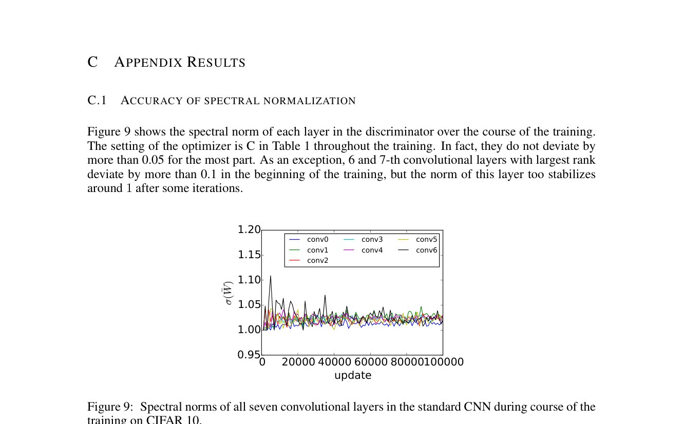
Figure 9: Spectral norms of all seven convolutional layers in the standard CNN during course of the training on CIFAR 10.
图 9:标准 CNN 在 CIFAR-10 训练过程中全部七个卷积层的谱范数。
C.2 Training Time
C.2 训练时间
| (a) CIFAR-10 (image size:) (b) STL-10 (images size:) Figure 10: Computational time for 100 updates. We set |
|---|
(a) CIFAR-10 (image size:)
| (a) CIFAR-10 (image size:) (b) STL-10 (images size:) 图 10:100 次更新的计算时间。我们设 |
|---|
(a) CIFAR-10 (image size:)
C.3 The effect of on spectral normalization and weight normalization
C.3 对谱归一化与权重归一化的影响
Figure 11 shows the effect of on the performance of weight normalization and spectral normalization. All results shown in Figure 11 follows setting D, except for the value of . For WN, the performance deteriorates with larger , which amounts to computing minimax with better accuracy. Our SN does not suffer from this unintended effect.
图 11 展示 对权重归一化与谱归一化表现的影响。图 11 所示全部结果除 外均沿用设置 D。对 WN,更大的 (相当于更精确地计算 minimax)会使表现变差;我们的 SN 不会遭受这种意外效应。
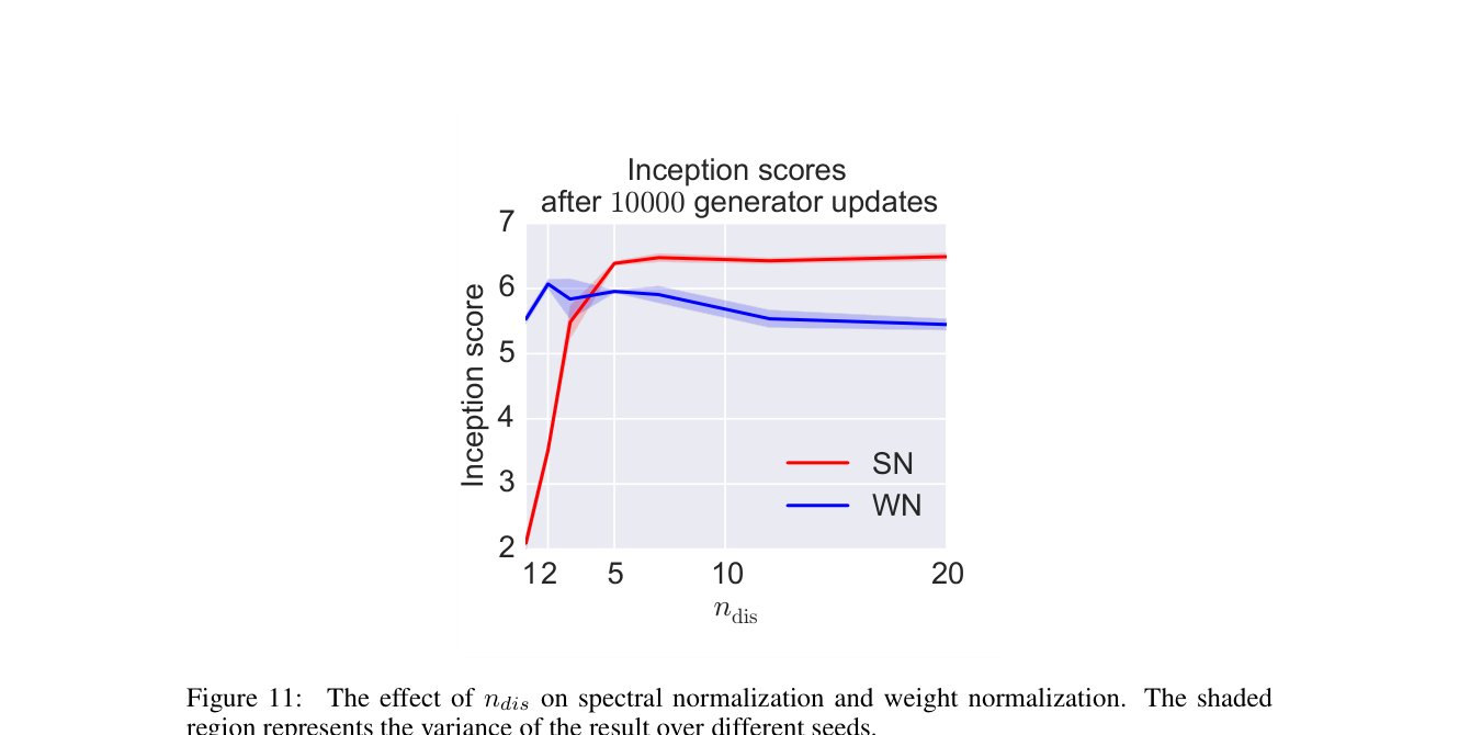
Figure 11: The effect of on spectral normalization and weight normalization. The shaded region represents the variance of the result over different seeds.
图 11: 对谱归一化与权重归一化的影响。阴影区域表示不同种子下结果的方差。
C.4 Generated Images on CIFAR10 with GAN-GP, Layer Normalization and Batch Normalization
C.4 CIFAR10 上 GAN-GP、层归一化与批归一化的生成图像
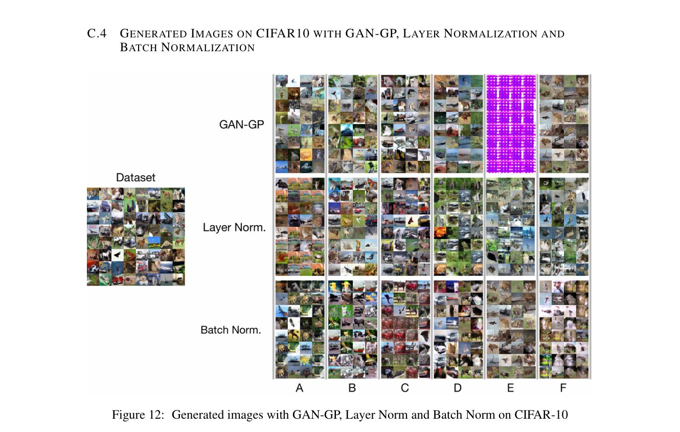
Figure 12: Generated images with GAN-GP, Layer Norm and Batch Norm on CIFAR-10
图 12:CIFAR-10 上 GAN-GP、层归一化与批归一化的生成图像
C.5 Image generation on Imagenet
C.5 ImageNet 上的图像生成
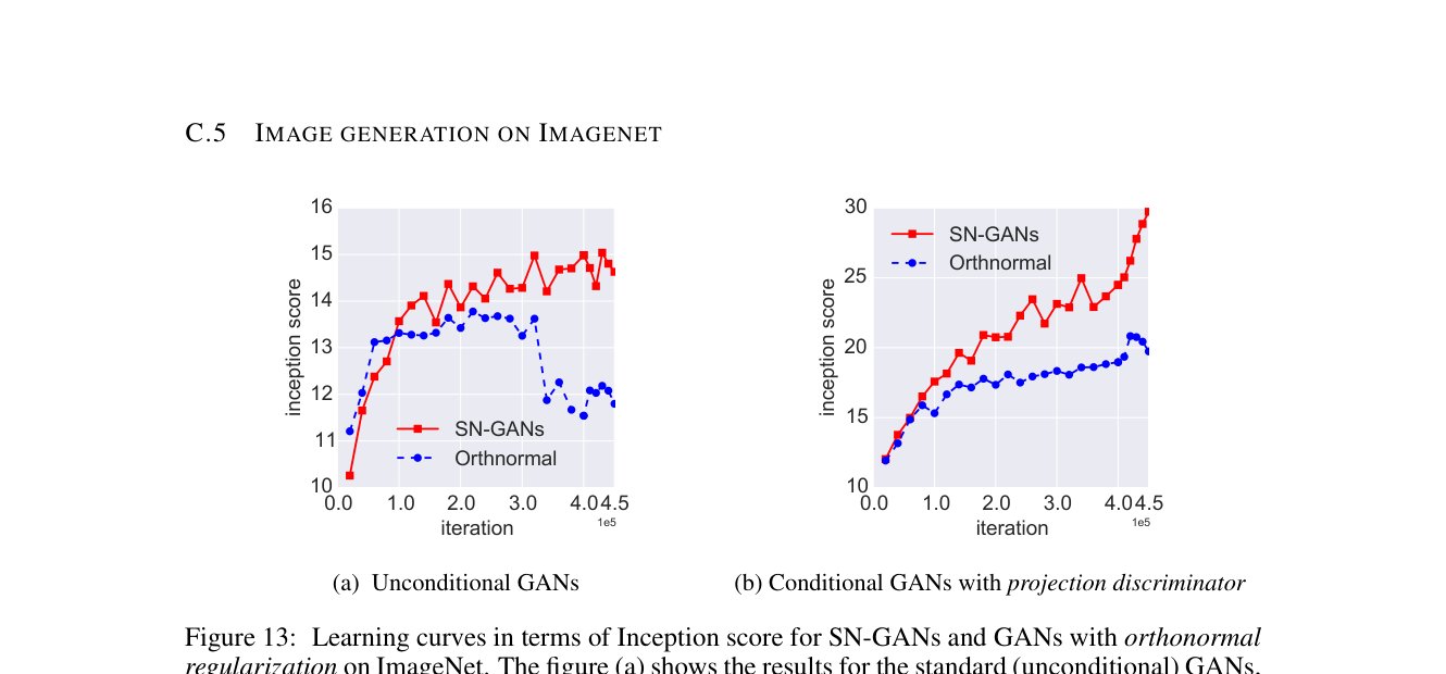
Figure 13: Unconditional GANs
图 13:无条件 GAN
Appendix D Spectral Normalization vs Other Regularization Techniques
附录 D 谱归一化与其他正则技术
This section is dedicated to the comparative study of spectral normalization and other regularization methods for discriminators. In particular, we will show that contemporary regularizations including weight normalization and weight clipping implicitly impose constraints on weight matrices that places unnecessary restriction on the search space of the discriminator. More specifically, we will show that weight normalization and weight clipping unwittingly favor low-rank weight matrices. This can force the trained discriminator to be largely dependent on select few features, rendering the algorithm to be able to match the model distribution with the target distribution only on very low dimensional feature space.
本节专门比较谱归一化与判别器上的其他正则方法。尤其将表明:包括权重归一化与权重裁剪在内的同期正则,会隐式对权重矩阵施加不必要地限制判别器搜索空间的约束。更具体地,我们将表明权重归一化与权重裁剪 无意中 偏好低秩权重矩阵。这会迫使训出的判别器很大程度上依赖少数选定特征,从而使算法只能在很低维的特征空间上匹配模型分布与目标分布。
D.1 Weight Normalization and Frobenius Normalization
D.1 权重归一化与 Frobenius 归一化
The weight normalization introduced by Salimans & Kingma 2016 is a method that normalizes the norm of each row vector in the weight matrix[^8]:
Salimans & Kingma 2016 引入的权重归一化,是把权重矩阵每行向量的 范数归一化[^8]:
where and are the th row vector of and , respectively.
其中 与 分别为 与 的第 行向量。
Still another technique to regularize the weight matrix is to use the Frobenius norm:
另一正则权重矩阵的技术是使用 Frobenius 范数:
where .
其中 。
Originally, these regularization techniques were invented with the goal of improving the generalization performance of supervised training Salimans & Kingma 2016; Arpit et al. 2016. However, recent works in the field of GANs Salimans et al. 2016; Xiang & Li 2017 found their another raison d’etat as a regularizer of discriminators, and succeeded in improving the performance of the original.
这些正则技术最初旨在提升有监督训练的泛化表现(Salimans & Kingma 2016;Arpit et al. 2016)。然而 GAN 领域近期工作(Salimans et al. 2016;Xiang & Li 2017)发现它们作为判别器正则的另一用途,并成功改进了原方法表现。
These methods in fact can render the trained discriminator to be -Lipschitz for a some prescribed and achieve the desired effect to a certain extent. However, weight normalization (25) imposes the following implicit restriction on the choice of :
这些方法确实可使训出的判别器 对某指定 成为 -Lipschitz,并在一定程度上达到期望效果。然而权重归一化 (25) 对 的选择施加如下隐式限制:
where is a -th singular value of matrix . The above equation holds because . Under this restriction, the norm for a fixed unit vector is maximized at when and for , which means that is of rank one. Using such corresponds to using only one feature to discriminate the model probability distribution from the target. Similarly, Frobenius normalization requires , and the same argument as above follows.
其中 为矩阵 的第 个奇异值。上式成立是因为 。在此限制下,对固定单位向量 , 在 且 ()时取最大 ,这意味着 秩为一。使用这样的 相当于只用一个特征区分模型概率分布与目标。类似地,Frobenius 归一化要求 ,上述论证同样成立。
Here, we see a critical problem in these two regularization methods. In order to retain as much norm of the input as possible and hence to make the discriminator more sensitive, one would hope to make the norm of large. For weight normalization, however, this comes at the cost of reducing the rank and hence the number of features to be used for the discriminator. Thus, there is a conflict of interests between weight normalization and our desire to use as many features as possible to distinguish the generator distribution from the target distribution. The former interest often reigns over the other in many cases, inadvertently diminishing the number of features to be used by the discriminators. Consequently, the algorithm would produce a rather arbitrary model distribution that matches the target distribution only at select few features.
至此可见这两种正则方法的关键问题。为尽可能保留输入范数、从而使判别器更敏感,人们希望 较大。但对权重归一化而言,这要以降低秩、从而减少判别可用特征数为代价。于是权重归一化与「尽量用多特征区分生成器分布与目标」的愿望冲突。前者常常压倒后者,无意中削弱判别器可用特征数。结果算法会产出相当任意的模型分布,只在少数选定特征上匹配目标。
Our spectral normalization, on the other hand, do not suffer from such a conflict in interest. Note that the Lipschitz constant of a linear operator is determined only by the maximum singular value. In other words, the spectral norm is independent of rank. Thus, unlike the weight normalization, our spectral normalization allows the parameter matrix to use as many features as possible while satisfying local -Lipschitz constraint. Our spectral normalization leaves more freedom in choosing the number of singular components (features) to feed to the next layer of the discriminator.
我们的谱归一化则不会陷入此类利益冲突。注意线性算子的 Lipschitz 常数只由最大奇异值决定;换言之,谱范数与秩无关。因此与权重归一化不同,谱归一化允许参数矩阵在满足局部 1-Lipschitz 约束的同时尽可能多用特征。谱归一化在选择送入判别器下一层的奇异分量(特征)数目上留下更多自由。
To see this more visually, we refer the reader to Figure (16). Note that spectral normalization allows for a wider range of choices than weight normalization.
为更直观地看到这一点,请读者参阅图 (16)。注意谱归一化允许的选择范围比权重归一化更宽。
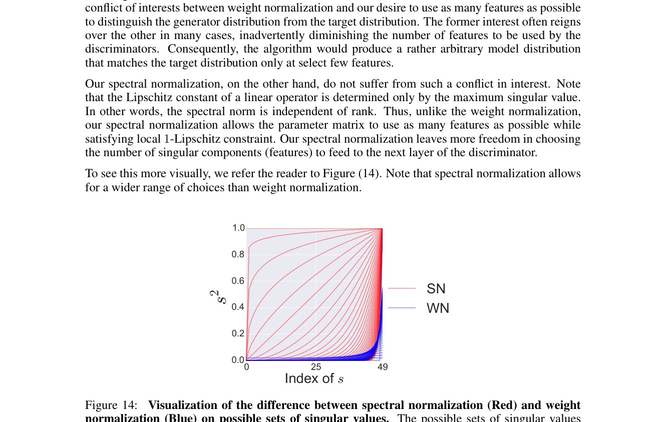
Figure 16: Visualization of the difference between spectral normalization (Red) and weight normalization (Blue) on possible sets of singular values. The possible sets of singular values plotted in increasing order for weight normalization (Blue) and for spectral normalization (Red). For the set of singular values permitted under the spectral normalization condition, we scaled by so that its spectral norm is exactly 1. By the definition of the weight normalization, the area under the blue curves are all bound to be . Note that the range of choice for the weight normalization is small.
图 16:谱归一化(红)与权重归一化(蓝)在可能奇异值集合上的差异可视化。 按递增顺序画出权重归一化(蓝)与谱归一化(红)允许的奇异值集合。对谱归一化条件下允许的奇异值集合,我们将 缩放 ,使其谱范数恰好为 1。按权重归一化定义,蓝色曲线下面积均须为 。注意权重归一化的可选范围较小。
In summary, weight normalization and Frobenius normalization favor skewed distributions of singular values, making the column spaces of the weight matrices lie in (approximately) low dimensional vector spaces. On the other hand, our spectral normalization does not compromise the number of feature dimensions used by the discriminator. In fact, we will experimentally show that GANs trained with our spectral normalization can generate a synthetic dataset with wider variety and higher inception score than the GANs trained with other two regularization methods.
总之,权重归一化与 Frobenius 归一化偏好偏斜的奇异值分布,使权重矩阵列空间落在(近似)低维向量空间。相反,谱归一化不牺牲判别器使用的特征维数。事实上我们将实验表明:用谱归一化训练的 GAN 比用另外两种正则训练的 GAN,能生成更多样、inception score 更高的合成数据。
D.2 Weight Clipping
D.2 权重裁剪
Still another regularization technique is weight clipping introduced by Arjovsky et al. 2017 in their training of Wasserstein GANs. Weight clipping simply truncates each element of weight matrices so that its absolute value is bounded above by a prescribed constant . Unfortunately, weight clipping suffers from the same problem as weight normalization and Frobenius normalization. With weight clipping with the truncation value , the value for a fixed unit vector is maximized when the rank of is again one, and the training will again favor the discriminators that use only select few features. Gulrajani et al. 2017 refers to this problem as capacity underuse problem. They also reported that the training of WGAN with weight clipping is slower than that of the original DCGAN Radford et al. 2016.
另一正则技术是 Arjovsky et al. 2017 在训练 Wasserstein GAN 时引入的 权重裁剪:简单截断权重矩阵各元素,使其绝对值不超过指定常数 。不幸的是,权重裁剪与权重归一化、Frobenius 归一化有同样问题。以截断值 做权重裁剪时,对固定单位向量 , 再次在 秩为一时取最大,训练仍会偏好只使用少数选定特征的判别器。Gulrajani et al. 2017 称之为容量利用不足问题。他们还报告带权重裁剪的 WGAN 训练慢于原版 DCGAN(Radford et al. 2016)。
D.3 Singular Value Clipping and Singular Value Constraint
D.3 奇异值裁剪与奇异值约束
One direct and straightforward way of controlling the spectral norm is to clip the singular values Saito et al. 2017, Jia et al. 2017. This approach, however, is computationally heavy because one needs to implement singular value decomposition in order to compute all the singular values.
控制谱范数的一种直接做法是裁剪奇异值(Saito et al. 2017;Jia et al. 2017)。然而该方法计算沉重,因为需要实现奇异值分解以计算全部奇异值。
A similar but less obvious approach is to parametrize as follows from the get-go and train the discriminators with this constrained parametrization:
一种类似但不那么显然的做法,是从一开始就把 参数化为如下形式,并在该约束参数化下训练判别器:
where , , and is a diagonal matrix. However, it is not a simple task to train this model while remaining absolutely faithful to this parametrization constraint. Our spectral normalization, on the other hand, can carry out the updates with relatively low computational cost without compromising the normalization constraint.
其中 ,, 为对角矩阵。然而在完全忠实于该参数化约束的前提下训练该模型并不简单。相反,谱归一化可以相对低的计算开销完成更新,且不牺牲归一化约束。
D.4 WGAN with Gradient Penalty (WGAN-GP)
D.4 带梯度惩罚的 WGAN(WGAN-GP)
Recently, Gulrajani et al. 2017 introduced a technique to enhance the stability of the training of Wasserstein GANs Arjovsky et al. 2017. In their work, they endeavored to place -Lipschitz constraint (5) on the discriminator by augmenting the adversarial loss function with the following regularizer function:
近来 Gulrajani et al. 2017 引入技术以增强 Wasserstein GAN(Arjovsky et al. 2017)训练的稳定性。他们通过在对抗损失函数上附加如下正则函数,试图对判别器施加 -Lipschitz 约束 (5):
where is a balancing coefficient and is:
其中 为平衡系数, 为:
Using this augmented objective function, Gulrajani et al. 2017 succeeded in training a GAN based on ResNet He et al. 2016 with an impressive performance. The advantage of their method in comparison to spectral normalization is that they can impose local -Lipschitz constraint directly on the discriminator function without a rather round-about layer-wise normalization. This suggest that their method is less likely to underuse the capacity of the network structure.
借助该增强目标,Gulrajani et al. 2017 成功训练了基于 ResNet(He et al. 2016)且表现令人印象深刻的 GAN。相对谱归一化,其优势是可直接对判别器函数施加局部 1-Lipschitz 约束,而无需较迂回的逐层归一化。这表明他们的方法较不易造成网络结构容量利用不足。
At the same time, this type of method that penalizes the gradients at sample points suffers from the obvious problem of not being able to regularize the function at the points outside of the support of the current generative distribution. In fact, the generative distribution and its support gradually changes in the course of the training, and this can destabilize the effect of the regularization itself.
与此同时,这类在样本点 惩罚梯度的方法有一明显问题:无法正则当前生成分布支撑之外的点上的函数。事实上,训练过程中生成分布及其支撑逐渐变化,可能使正则效果本身不稳定。
On the contrary, our spectral normalization regularizes the function itself, and the effect of the regularization is more stable with respect to the choice of the batch. In fact, we observed in the experiment that a high learning rate can destabilize the performance of WGAN-GP. Training with our spectral normalization does not falter with aggressive learning rate.
相反,谱归一化正则的是函数本身,正则效果相对 batch 选择更稳定。事实上实验中我们观察到高学习率会使 WGAN-GP 表现不稳;用谱归一化训练时,激进学习率也不易动摇。
Moreover, WGAN-GP requires more computational cost than our spectral normalization with single-step power iteration, because the computation of requires one whole round of forward and backward propagation. In Figure 10, we compare the computational cost of the two methods for the same number of updates.
此外,相对单步幂迭代的谱归一化,WGAN-GP 计算更贵,因为计算 需要一整轮前向与反向。图 10 按相同更新次数对比两种方法的计算开销。
Having said that, one shall not rule out the possibility that the gradient penalty can compliment spectral normalization and vice versa. Because these two methods regularizes discriminators by completely different means, and in the experiment section, we actually confirmed that combination of WGAN-GP and reparametrization with spectral normalization improves the quality of the generated examples over the baseline (WGAN-GP only).
话虽如此,不应排除梯度惩罚可与谱归一化互补的可能性。二者以完全不同的方式正则判别器;实验部分我们实际上确认:把 WGAN-GP 与谱归一化重参数化组合,相对仅用 WGAN-GP 的基线,可改进生成样本质量。
Appendix E Reparametrization motivated by the spectral normalization
附录 E 由谱归一化启发的重参数化
We can take advantage of the regularization effect of the spectral normalization we saw above to develop another algorithm. Let us consider another parametrization of the weight matrix of the discriminator given by: \EmphEqMainEnv ~ W := γ ¯ WSN \endEmphEqMainEnv where is a scalar variable to be learned. This parametrization compromises the -Lipschitz constraint at the layer of interest, but gives more freedom to the model while keeping the model from becoming degenerate. For this reparametrization, we need to control the Lipschitz condition by other means, such as the gradient penalty Gulrajani et al. 2017. Indeed, we can think of analogous versions of reparametrization by replacing $\bar{W}{\rm SN}Wnormalized by other criterions. The extension of this form is not new. In Salimans & Kingma 2016, they originally introduced weight normalization in order to derive the reparametrization of the form (E) with\bar{W}{\rm SN}W{\rm WN}\gamma$.
我们可以利用上文所见谱归一化的正则效应,发展另一算法。考虑判别器权重矩阵的另一参数化:,其中 为待学习标量。该参数化在所关注层上放松了 1-Lipschitz 约束,但在防止模型退化的同时给模型更多自由。对此重参数化,需用其他手段(如梯度惩罚,Gulrajani et al. 2017)控制 Lipschitz 条件。确实,也可设想用其他准则归一化的 替换 (E) 中的 ,得到类似重参数化。这一形式的扩展并非新事:Salimans & Kingma 2016 最初引入权重归一化,正是为了导出用 替换 并把 向量化的形式 (E)。
E.1 Experiments: Comparison of Reparametrization with different normalization methods
E.1 实验:不同归一化方法重参数化的对比
In this part of the addendum, we experimentally compare the reparametrizations derived from two different normalization methods (weight normalization and spectral normalization). We tested the reprametrization methods for the training of the discriminator of WGAN-GP. For the architecture of the network in WGAN-GP, we used the same CNN we used in the previous section. For the ResNet-based CNN, we used the same architecture provided by Gulrajani et al. 2017 [^9].
本附录这部分实验对比由两种不同归一化方法(权重归一化与谱归一化)导出的重参数化。我们在 WGAN-GP 判别器训练上测试重参数化方法。WGAN-GP 网络结构使用与前节相同的 CNN;基于 ResNet 的 CNN 使用 Gulrajani et al. 2017 提供的相同结构[^9]。
Tables 7, 8 summarize the result. We see that our method significantly improves the inception score from the baseline on the regular CNN, and slightly improves the score on the ResNet based CNN.
表 7、8 总结结果。可见本方法在常规 CNN 上相对基线显著提升 inception score,在基于 ResNet 的 CNN 上略有提升。
Figure 17 shows the learning curves of (a) critic losses, on train and validation sets and (b) the inception scores with different reparametrization methods. We can see the beneficial effect of spectral normalization in the learning curve of the discriminator as well. We can verify in the figure 17(a) that the discriminator with spectral normalization overfits less to the training dataset than the discriminator without reparametrization and with weight normalization, The effect of overfitting can be observed on inception score as well, and the final score with spectral normalization is better than the others. As for the best inception score achieved in the course of the training, spectral normalization achieved 7.28, whereas the spectral normalization and vanilla normalization achieved 7.04 and 6.69, respectively.
图 17 展示 (a) 训练与验证集上 critic 损失与 (b) 不同重参数化方法下 inception score 的学习曲线。也可在判别器学习曲线上看到谱归一化的益处。图 17(a) 可验证:带谱归一化的判别器相对无重参数化与带权重归一化的判别器,对训练数据过拟合更少。过拟合效应也可在 inception score 上观察到,谱归一化的最终分数优于其他。就训练过程中达到的最佳 inception score 而言,谱归一化为 7.28,而权重归一化与无归一化分别为 7.04 与 6.69。
| Method | Inception score | FID |
|---|---|---|
| WGAN-GP (Standard CNN, Baseline) | 6.68.06 | 40.1 |
| w/ Frobenius Norm. | N/A∗ | N/A∗ |
| w/ Weight Norm. | 6.36.04 | 42.4 |
| w/ Spectral Norm. | 7.20.08 | 32.0 |
| (WGAN-GP, ResNet, Gulrajani et al. 2017) | 7.86.08 | |
| WGAN-GP (ResNet, Baseline) | 7.80.11 | 24.5 |
| w/ Spectral norm. | 7.85.06 | 23.6 |
| w/ Spectral norm. (1.5x feature maps in ) | 7.96.06 | 22.5 |
Table 7: Inception scores with different reparametrization mehtods on CIFAR10 without label supervisions. (*)We reported N/A for the inception score and FID of Frobenius normalization because the training collapsed at the early stage.
| Method | Inception score | FID |
|---|---|---|
| WGAN-GP (Standard CNN, Baseline) | 6.68.06 | 40.1 |
| w/ Frobenius Norm. | N/A∗ | N/A∗ |
| w/ Weight Norm. | 6.36.04 | 42.4 |
| w/ Spectral Norm. | 7.20.08 | 32.0 |
| (WGAN-GP, ResNet, Gulrajani et al. 2017) | 7.86.08 | |
| WGAN-GP (ResNet, Baseline) | 7.80.11 | 24.5 |
| w/ Spectral norm. | 7.85.06 | 23.6 |
| w/ Spectral norm. (1.5x feature maps in ) | 7.96.06 | 22.5 |
表 7:CIFAR10 无标签监督下不同重参数化方法的 inception score。(*)Frobenius 归一化因训练早期崩溃,inception score 与 FID 记为 N/A。
| Method (ResNet) | Inception score | FID |
|---|---|---|
| (AC-WGAN-GP, Gulrajani et al. 2017) | 8.42.10 | |
| AC-WGAN-GP (Baseline) | 8.29.12 | 19.5 |
| w/ Spectral norm. | 8.59.12 | 18.6 |
| w/ Spectral norm. (1.5x feature maps in ) | 8.60.08 | 17.5 |
Table 8: Inception scores and FIDs with different reparametrization methods on CIFAR10 with the label supervision, by auxiliary classifier Odena et al. 2017.
| Method (ResNet) | Inception score | FID |
|---|---|---|
| (AC-WGAN-GP, Gulrajani et al. 2017) | 8.42.10 | |
| AC-WGAN-GP (Baseline) | 8.29.12 | 19.5 |
| w/ Spectral norm. | 8.59.12 | 18.6 |
| w/ Spectral norm. (1.5x feature maps in ) | 8.60.08 | 17.5 |
表 8:CIFAR10 带标签监督(辅助分类器,Odena et al. 2017)时不同重参数化方法的 inception score 与 FID。
(a) Critic loss
(a) Critic 损失
Appendix F The gradient of General Normalization Method
附录 F 一般归一化方法的梯度
Let us denote to be the normalized weight where to be a scalar normalized coefficient (e.g. Spectral norm or Frobenius norm). In general, we can write the derivative of loss with respect to unnormalized weight as follows:
记 为归一化权重,其中 为标量归一化系数(例如谱范数或 Frobenius 范数)。一般地,损失对未归一化权重 的导数可写为:
where and . The gradient is calculated by where , is the hidden node in the network to be transformed by and represents empirical expectation over the mini-batch. When , the derivative is:
其中 ,。梯度 由 计算,其中 , 为网络中将被 变换的隐节点, 表示 mini-batch 上的经验期望。当 时,导数为:
and when ,
而当 时,
Notice that, at least for the case or , the point of this gradient is given by :
注意至少对 或 ,该梯度的驻点由下式给出:
where
其中