SlowFast Networks for Video Recognition
SlowFast Networks for Video Recognition
Christoph Feichtenhofer Haoqi Fan Jitendra Malik Kaiming He Affiliation: Facebook AI Research (FAIR)
Abstract
摘要
We present SlowFast networks for video recognition. Our model involves (i) a Slow pathway, operating at low frame rate, to capture spatial semantics, and (ii) a Fast pathway, operating at high frame rate, to capture motion at fine temporal resolution. The Fast pathway can be made very lightweight by reducing its channel capacity, yet can learn useful temporal information for video recognition. Our models achieve strong performance for both action classification and detection in video, and large improvements are pin-pointed as contributions by our SlowFast concept. We report state-of-the-art accuracy on major video recognition benchmarks, Kinetics, Charades and AVA. Code has been made available at: https://github.com/facebookresearch/SlowFast.
我们提出用于视频识别的 SlowFast 网络。模型包含:(i) 以低帧率运行的 Slow 通路,用于捕获空间语义;(ii) 以高帧率运行的 Fast 通路,用于在细时间分辨率上捕获运动。Fast 通路可通过降低通道容量做得很轻,却仍能学到对视频识别有用的时间信息。我们的模型在动作分类与检测上都表现强劲,且大量提升可明确归因于 SlowFast 设计。我们在主要视频识别基准 Kinetics、Charades 与 AVA 上报告当时最好准确率。代码见:https://github.com/facebookresearch/SlowFast。
1 Introduction
1 引言
It is customary in the recognition of images to treat the two spatial dimensions and symmetrically. This is justified by the statistics of natural images, which are to a first approximation isotropic—all orientations are equally likely—and shift-invariant Ruderman1994; Huang1999. But what about video signals ? Motion is the spatiotemporal counterpart of orientation Adelson1985, but all spatiotemporal orientations are not equally likely. Slow motions are more likely than fast motions (indeed most of the world we see is at rest at a given moment) and this has been exploited in Bayesian accounts of how humans perceive motion stimuli Weiss2002. For example, if we see a moving edge in isolation, we perceive it as moving perpendicular to itself, even though in principle it could also have an arbitrary component of movement tangential to itself (the aperture problem in optical flow). This percept is rational if the prior favors slow movements.
识别图像 时,习惯把两个空间维 与 对称对待。这由自然图像统计支持:一阶近似各向同性——各方向同等可能——且平移不变 Ruderman1994;Huang1999。但视频信号 呢?运动是取向的时空对应物 Adelson1985,但并非所有时空取向同等可能。慢运动比快运动更常见(的确,我们所见世界在给定时刻大多静止),贝叶斯视角下人类如何感知运动刺激也利用了这一点 Weiss2002。例如,单独看到一条运动边缘时,我们会感知它沿垂直于自身的方向运动,尽管原则上还可有任意切向分量(光流中的孔径问题)。若先验偏好慢运动,这一感知是合理的。
If all spatiotemporal orientations are not equally likely, then there is no reason for us to treat space and time symmetrically, as is implicit in approaches to video recognition based on spatiotemporal convolutions Tran2015; Carreira2017. We might instead “factor” the architecture to treat spatial structures and temporal events separately. For concreteness, let us study this in the context of recognition. The categorical spatial semantics of the visual content often evolve slowly. For example, waving hands do not change their identity as “hands” over the span of the waving action, and a person is always in the “person” category even though he/she can transit from walking to running. So the recognition of the categorical semantics (as well as their colors, textures, lighting etc.) can be refreshed relatively slowly. On the other hand, the motion being performed can evolve much faster than their subject identities, such as clapping, waving, shaking, walking, or jumping. It can be desired to use fast refreshing frames (high temporal resolution) to effectively model the potentially fast changing motion.
若并非所有时空取向同等可能,就没有理由像基于时空卷积的视频识别方法那样,隐含地把空间与时间对称对待 Tran2015;Carreira2017。我们或许应「分解」架构,分别处理空间结构与时间事件。具体地,放在识别语境下:视觉内容的类别空间语义往往缓慢演化。例如挥手过程中,「手」的身份不变;人从走到跑,「人」这一类也不变。因此类别语义(及其颜色、纹理、光照等)可以相对慢地刷新。另一方面,所执行的动作可比主体身份演化得快得多,如鼓掌、挥手、抖动、走或跳。可能希望用快刷新帧(高时间分辨率)来有效建模潜在的快速变化运动。
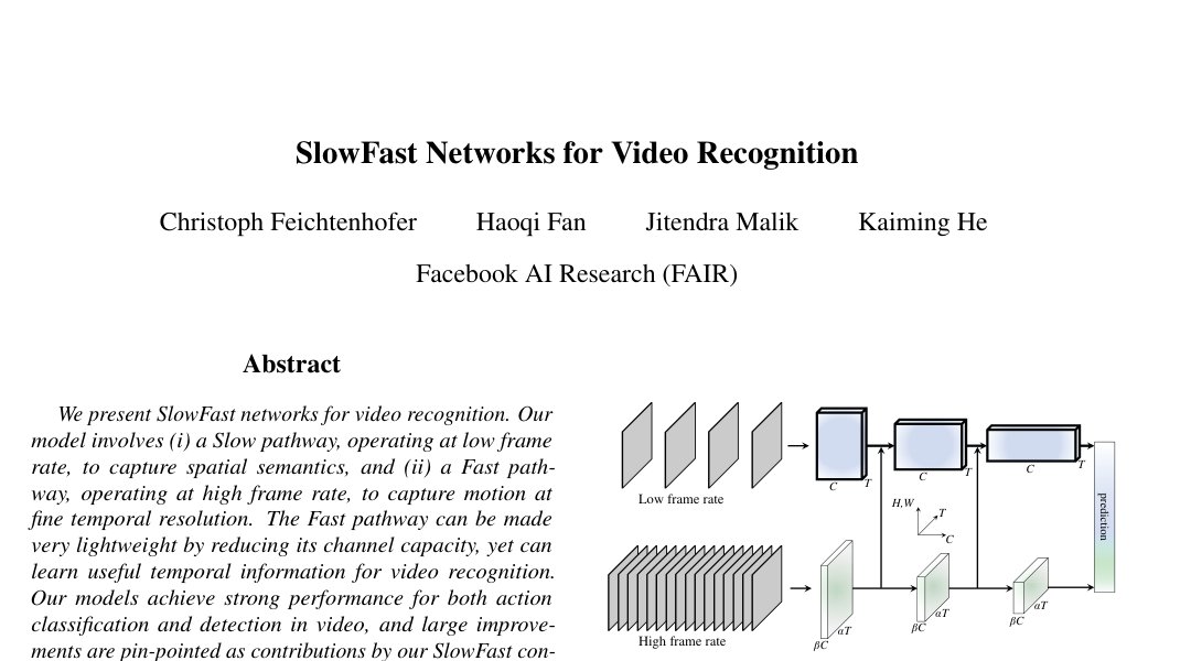
Figure 1: A SlowFast network has a low frame rate, low temporal resolution Slow pathway and a high frame rate, higher temporal resolution Fast pathway. The Fast pathway is lightweight by using a fraction (, e.g., 1/8) of channels. Lateral connections fuse them.
图 1:SlowFast 网络具有低帧率、低时间分辨率的 Slow 通路,以及帧率高 倍、时间分辨率更高的 Fast 通路。Fast 通路通道数仅为分数(,例如 1/8),因而很轻。侧向连接融合两通路。
Based on this intuition, we present a two-pathway SlowFast model for video recognition (Fig. 1). One pathway is designed to capture semantic information that can be given by images or a few sparse frames, and it operates at low frame rates and slow refreshing speed. In contrast, the other pathway is responsible for capturing rapidly changing motion, by operating at fast refreshing speed and high temporal resolution. Despite its high temporal rate, this pathway is made very lightweight, e.g., 20% of total computation. This is because this pathway is designed to have fewer channels and weaker ability to process spatial information, while such information can be provided by the first pathway in a less redundant manner. We call the first a Slow pathway and the second a Fast pathway, driven by their different temporal speeds. The two pathways are fused by lateral connections.
基于这一直觉,我们提出用于视频识别的双通路 SlowFast 模型(图 1)。一条通路用于捕获可由图像或少量稀疏帧给出的语义信息,以低帧率与慢刷新速度运行。另一条通路负责捕获快速变化的运动,以快刷新与高时间分辨率运行。尽管时间率高,该通路仍做得很轻,例如约占总算力约 20%。因为它通道更少、处理空间信息的能力更弱,而这些信息可由第一条通路以更少冗余的方式提供。按其不同时间速度,我们称前者为 Slow 通路、后者为 Fast 通路。两通路由侧向连接融合。
Our conceptual idea leads to flexible and effective designs for video models. The Fast pathway, due to its lightweight nature, does not need to perform any temporal pooling—it can operate on high frame rates for all intermediate layers and maintain temporal fidelity. Meanwhile, thanks to the lower temporal rate, the Slow pathway can be more focused on the spatial domain and semantics. By treating the raw video at different temporal rates, our method allows the two pathways to have their own expertise on video modeling.
这一概念带来灵活且有效的视频模型设计。Fast 通路因其轻量不必做任何时间池化——可在所有中间层保持高帧率并维持时间保真。同时,得益于更低时间率,Slow 通路可更专注于空间域与语义。通过对原始视频采用不同时间率,我们的方法让两通路各自专长于视频建模。
There is another well known architecture for video recognition which has a two-stream design Simonyan2014, but provides conceptually different perspectives. The Two-Stream method Simonyan2014 has not explored the potential of different temporal speeds, a key concept in our method. The two-stream method adopts the same backbone structure to both streams, whereas our Fast pathway is more lightweight. Our method does not compute optical flow, and therefore, our models are learned end-to-end from the raw data. In our experiments we observe that the SlowFast network is empirically more effective.
视频识别另有著名的双流架构 Simonyan2014,但视角概念上不同。双流方法 Simonyan2014 并未探索不同时间速度这一我们方法的关键概念。双流对两路采用相同骨干,而我们的 Fast 通路更轻。我们的方法不计算光流,因此模型从原始数据端到端学习。实验中我们观察到 SlowFast 网络经验上更有效。
Our method is partially inspired by biological studies on the retinal ganglion cells in the primate visual system Hubel1965; Livingstone1988; Derrington1984; Felleman1991; VanEssen1994, though admittedly the analogy is rough and premature. These studies found that in these cells, 80% are Parvocellular (P-cells) and 15-20% are Magnocellular (M-cells). The M-cells operate at high temporal frequency and are responsive to fast temporal changes, but not sensitive to spatial detail or color. P-cells provide fine spatial detail and color, but lower temporal resolution, responding slowly to stimuli. Our framework is analogous in that: (i) our model has two pathways separately working at low and high temporal resolutions; (ii) our Fast pathway is designed to capture fast changing motion but fewer spatial details, analogous to M-cells; and (iii) our Fast pathway is lightweight, similar to the small ratio of M-cells. We hope these relations will inspire more computer vision models for video recognition.
我们的方法部分受到灵长类视觉系统视网膜神经节细胞生物学研究启发 Hubel1965;Livingstone1988;Derrington1984;Felleman1991;VanEssen1994,尽管类比粗略且尚早。这些研究发现,约 80% 为小细胞(P-cells),约 15–20% 为大细胞(M-cells)。M 细胞以高时间频率运行,对快速时间变化敏感,但对空间细节或颜色不敏感。P 细胞提供精细空间细节与颜色,但时间分辨率较低,对刺激响应较慢。我们的框架类比在于:(i) 模型有两条分别在低、高时间分辨率工作的通路;(ii) Fast 通路用于捕获快变运动但更少空间细节,类似 M 细胞;(iii) Fast 通路轻量,类似 M 细胞占比较小。希望这些关联能启发更多视频识别的计算机视觉模型。
We evaluate our method on the Kinetics-400 Kay2017, Kinetics-600 Carreira2018, Charades Sigurdsson2016 and AVA Gu2018 datasets. Our comprehensive ablation experiments on Kinetics action classification demonstrate the efficacy contributed by SlowFast. SlowFast networks set a new state-of-the-art on all datasets with significant gains to previous systems in the literature.
我们在 Kinetics-400 Kay2017、Kinetics-600 Carreira2018、Charades Sigurdsson2016 与 AVA Gu2018 上评估。Kinetics 动作分类上的全面消融表明 SlowFast 有效。SlowFast 网络在全部数据集上刷新最好结果,相对文献中先前系统有显著提升。
2 Related Work
2 相关工作
Spatiotemporal filtering.
Actions can be formulated as spatiotemporal objects and captured by oriented filtering in spacetime, as done by HOG3D Klaeser2008 and cuboids Dollar2005. 3D ConvNets Taylor2010; Tran2015; Carreira2017 extend 2D image models Krizhevsky2012; Simonyan2015; Szegedy2015; He2016 to the spatiotemporal domain, handling both spatial and temporal dimensions similarly. There are also related methods focusing on long-term filtering and pooling using temporal strides Varol2018; Feichtenhofer2016; Wang2016a; Zhou2017, as well as decomposing the convolutions into separate 2D spatial and 1D temporal filters Feichtenhofer2016a; Tran2018; Xie2018; Qiu2017.
时空滤波。
动作可表述为时空对象,并由时空中的取向滤波捕获,如 HOG3D Klaeser2008 与 cuboids Dollar2005。3D ConvNet Taylor2010;Tran2015;Carreira2017 把二维图像模型 Krizhevsky2012;Simonyan2015;Szegedy2015;He2016 扩展到时空域,对空间与时间维类似处理。也有相关方法用时间步长做长期滤波与池化 Varol2018;Feichtenhofer2016;Wang2016a;Zhou2017,以及把卷积分解为独立的二维空间与一维时间滤波 Feichtenhofer2016a;Tran2018;Xie2018;Qiu2017。
Beyond spatiotemporal filtering or their separable versions, our work pursuits a more thorough separation of modeling expertise by using two different temporal speeds.
在时空滤波或其可分离版本之外,我们的工作追求更彻底的建模专长分离:使用两种不同的时间速度。
Optical flow for video recognition.
There is a classical branch of research focusing on hand-crafted spatiotemporal features based on optical flow. These methods, including histograms of flow Laptev2008, motion boundary histograms Dalal2006, and trajectories Wang2013, had shown competitive performance for action recognition before the prevalence of deep learning.
用于视频识别的光流。
有一支经典研究聚焦基于光流的手工时空特征。这些方法——包括光流直方图 Laptev2008、运动边界直方图 Dalal2006 与轨迹 Wang2013——在深度学习普及前对动作识别表现有竞争力。
In the context of deep neural networks, the two-stream method Simonyan2014 exploits optical flow by viewing it as another input modality. This method has been a foundation of many competitive results in the literature Feichtenhofer2016a; Feichtenhofer2016; Wang2016a. However, it is methodologically unsatisfactory given that optical flow is a hand-designed representation, and two-stream methods are often not learned end-to-end jointly with the flow.
在深度神经网络语境下,双流方法 Simonyan2014 把光流当作另一种输入模态加以利用。该方法是文献中许多有竞争力结果的基础 Feichtenhofer2016a;Feichtenhofer2016;Wang2016a。但鉴于光流是手工表示,且双流方法往往不与光流联合端到端学习,这一做法在方法上并不令人满意。
3 SlowFast Networks
3 SlowFast 网络
SlowFast networks can be described as a single stream architecture that operates at two different framerates, but we use the concept of pathways to reflect analogy with the biological Parvo- and Magnocellular counterparts. Our generic architecture has a Slow pathway (Sec. 3.1) and a Fast pathway (Sec. 3.2), which are fused by lateral connections to a SlowFast network (Sec. 3.3). Fig. 1 illustrates our concept.
SlowFast 网络可描述为在两种帧率下运行的单流架构,但我们使用「通路」概念以对应生物学上的小细胞与大细胞。通用架构含 Slow 通路(第 3.1 节)与 Fast 通路(第 3.2 节),经侧向连接融合成 SlowFast 网络(第 3.3 节)。图 1 示意这一概念。
3.1 Slow pathway
3.1 Slow 通路
The Slow pathway can be any convolutional model (e.g., Feichtenhofer2016a; Tran2015; Carreira2017; Wang2018) that works on a clip of video as a spatiotemporal volume. The key concept in our Slow pathway is a large temporal stride on input frames, i.e., it processes only one out of frames. A typical value of we studied is 16—this refreshing speed is roughly 2 frames sampled per second for 30-fps videos. Denoting the number of frames sampled by the Slow pathway as , the raw clip length is frames.
Slow 通路可以是任意作用于视频片段时空体的卷积模型(例如 Feichtenhofer2016a;Tran2015;Carreira2017;Wang2018)。关键概念是对输入帧采用大时间步长 ,即只处理每隔 帧中的一帧。我们研究的典型取值为 16——对 30-fps 视频大致相当于每秒采 2 帧。记 Slow 通路采样帧数为 ,则原始片段长度为 帧。
3.2 Fast pathway
3.2 Fast 通路
In parallel to the Slow pathway, the Fast pathway is another convolutional model with the following properties.
与 Slow 通路并行,Fast 通路是另一卷积模型,具有以下性质。
High frame rate.
Our goal here is to have a fine representation along the temporal dimension. Our Fast pathway works with a small temporal stride of , where is the frame rate ratio between the Fast and Slow pathways. The two pathways operate on the same raw clip, so the Fast pathway samples frames, times denser than the Slow pathway. A typical value is in our experiments.
高帧率。
目标是在时间维上获得精细表示。Fast 通路以小时间步长 工作,其中 为 Fast 与 Slow 的帧率比。两通路作用于同一原始片段,故 Fast 采样 帧,比 Slow 密 倍。实验中典型取 。
The presence of is in the key of the SlowFast concept (Fig. 1, time axis). It explicitly indicates that the two pathways work on different temporal speeds, and thus drives the expertise of the two subnets instantiating the two pathways.
的存在是 SlowFast 概念的关键(图 1,时间轴)。它明确表明两通路工作在不同时间速度上,从而驱动实例化两通路的子网专长。
High temporal resolution features.
Our Fast pathway not only has a high input resolution, but also pursues high-resolution features throughout the network hierarchy. In our instantiations, we use no temporal downsampling layers (neither temporal pooling nor time-strided convolutions) throughout the Fast pathway, until the global pooling layer before classification. As such, our feature tensors always have frames along the temporal dimension, maintaining temporal fidelity as much as possible.
高时间分辨率特征。
Fast 通路不仅输入分辨率高,也追求贯穿网络层级的高分辨率特征。实例化中,直到分类前的全局池化之前,我们在 Fast 通路不使用时间下采样层(既无时间池化也无时间步长卷积)。因此特征张量在时间维上始终有 帧,尽量保持时间保真。
Low channel capacity.
Our Fast pathway also distinguishes with existing models in that it can use significantly lower channel capacity to achieve good accuracy for the SlowFast model. This makes it lightweight.
低通道容量。
Fast 通路与现有模型的另一区别是:可用显著更低的通道容量,仍为 SlowFast 模型取得良好准确率。这使它轻量。
In a nutshell, our Fast pathway is a convolutional network analogous to the Slow pathway, but has a ratio of () channels of the Slow pathway. The typical value is in our experiments. Notice that the computation (floating-number operations, or FLOPs) of a common layer is often quadratic in term of its channel scaling ratio. This is what makes the Fast pathway more computation-effective than the Slow pathway. In our instantiations, the Fast pathway typically takes 20% of the total computation. Interestingly, as mentioned in Sec. 1, evidence suggests that 15-20% of the retinal cells in the primate visual system are M-cells (that are sensitive to fast motion but not color or spatial detail).
简言之,Fast 通路是类似 Slow 的卷积网络,但通道数为 Slow 的比例 ()。实验中典型取 。注意常见层的计算量(浮点运算,FLOPs)对通道缩放比往往是二次的。这正是 Fast 比 Slow 更省算力之处。实例化中,Fast 通常约占总算力 20%。有趣的是,如第 1 节所述,证据表明灵长类视觉系统中约 15–20% 的视网膜细胞是对快运动敏感、对颜色或空间细节不敏感的 M 细胞。
The low channel capacity can also be interpreted as a weaker ability of representing spatial semantics. Technically, our Fast pathway has no special treatment on the spatial dimension, so its spatial modeling capacity should be lower than the Slow pathway because of fewer channels. The good results of our model suggest that it is a desired tradeoff for the Fast pathway to weaken its spatial modeling ability while strengthening its temporal modeling ability.
低通道容量也可解读为表示空间语义的能力更弱。技术上,Fast 通路对空间维无特殊处理,因通道更少,其空间建模能力应弱于 Slow。良好结果表明:让 Fast 削弱空间建模、加强时间建模,是理想折中。
Motivated by this interpretation, we also explore different ways of weakening spatial capacity in the Fast pathway, including reducing input spatial resolution and removing color information. As we will show by experiments, these versions can all give good accuracy, suggesting that a lightweight Fast pathway with less spatial capacity can be made beneficial.
受此解读启发,我们也探索在 Fast 通路削弱空间能力的其他方式,包括降低输入空间分辨率与去除颜色信息。实验将表明这些版本都能给出良好准确率,说明空间能力较弱的轻量 Fast 通路可以有益。
3.3 Lateral connections
3.3 侧向连接
The information of the two pathways is fused, so one pathway is not unaware of the representation learned by the other pathway. We implement this by lateral connections, which have been used to fuse optical flow-based, two-stream networks Feichtenhofer2016a; Feichtenhofer2016. In image object detection, lateral connections Lin2017 are a popular technique for merging different levels of spatial resolution and semantics.
两通路的信息被融合,使一条通路不会对另一条所学表示一无所知。我们用侧向连接实现,此前已用于融合基于光流的双流网络 Feichtenhofer2016a;Feichtenhofer2016。在图像目标检测中,侧向连接 Lin2017 是合并不同空间分辨率与语义层级的常用技巧。
Similar to Feichtenhofer2016a; Lin2017, we attach one lateral connection between the two pathways for every “stage" (Fig. 1). Specifically for ResNets He2016, these connections are right after pool1, res2, res3, and res4. The two pathways have different temporal dimensions, so the lateral connections perform a transformation to match them (detailed in Sec. 3.4). We use unidirectional connections that fuse features of the Fast pathway into the Slow one (Fig. 1). We have experimented with bidirectional fusion and found similar results.
类似 Feichtenhofer2016a;Lin2017,我们在两通路每个「阶段」之间挂一条侧向连接(图 1)。对 ResNet He2016,这些连接正好在 pool1、res2、res3、res4 之后。两通路时间维不同,侧向连接做变换以匹配(第 3.4 节详述)。我们采用单向连接,把 Fast 通路特征融进 Slow(图 1)。我们也试过双向融合,结果相近。
Finally, a global average pooling is performed on each pathway’s output. Then two pooled feature vectors are concatenated as the input to the fully-connected classifier layer.
最后,对每条通路的输出做全局平均池化,再把两个池化特征向量拼接,作为全连接分类层的输入。
| stage | Slow pathway | Fast pathway | output sizes |
|---|---|---|---|
| raw clip | - | - | 64224 |
| data layer | stride 16, 1 | stride 2, 1 | \begin{array}[]{c}\text{\emph{Slow}}:\text{{4}\times{}^{\text{2}}}\\[-0.85005pt] \text{\emph{Fast}}:\text{{\color[rgb]{0.4727,0.6992,0.5}{32}}\times{}^{\text{2}}}\end{array} |
| conv1 | 17, 64 | 57, 8 | \begin{array}[]{c}\text{\emph{Slow}}:\text{{4}\times{}^{\text{2}}}\\[-0.85005pt] \text{\emph{Fast}}:\text{{\color[rgb]{0.4727,0.6992,0.5}{32}}\times{}^{\text{2}}}\end{array} |
| stride 1, 2 | stride 1, 2 | ||
| pool1 | 13 max | 13 max | \begin{array}[]{c}\text{\emph{Slow}}:\text{{4}\times{}^{\text{2}}}\\[-0.85005pt] \text{\emph{Fast}}:\text{{\color[rgb]{0.4727,0.6992,0.5}{32}}\times{}^{\text{2}}}\end{array} |
| stride 1, 2 | stride 1, 2 | ||
| res2 | \left[\begin{array}[]{c}\text{1\times{}^{\text{2}}, {64}}\\[-0.85005pt] \text{1\times{}^{\text{2}}, {64}}\\[-0.85005pt] \text{1\times{}^{\text{2}}, {256}}\end{array}\right]3 | \left[\begin{array}[]{c}\text{\lx@text@underline{3\times{}^{\text{2}}}, {\color[rgb]{1,0.5,0}8}}\\[-0.85005pt] \text{1\times{}^{\text{2}}, {\color[rgb]{1,0.5,0}8}}\\[-0.85005pt] \text{1\times{}^{\text{2}}, {\color[rgb]{1,0.5,0}32}}\end{array}\right]3 | \begin{array}[]{c}\text{\emph{Slow}}:\text{{4}\times{}^{\text{2}}}\\[-0.85005pt] \text{\emph{Fast}}:\text{{\color[rgb]{0.4727,0.6992,0.5}{32}}\times{}^{\text{2}}}\end{array} |
| res3 | \left[\begin{array}[]{c}\text{1\times{}^{\text{2}}, {128}}\\[-0.85005pt] \text{1\times{}^{\text{2}}, {128}}\\[-0.85005pt] \text{1\times{}^{\text{2}}, {512}}\end{array}\right]4 | \left[\begin{array}[]{c}\text{\lx@text@underline{3\times{}^{\text{2}}}, {\color[rgb]{1,0.5,0}16}}\\[-0.85005pt] \text{1\times{}^{\text{2}}, {\color[rgb]{1,0.5,0}16}}\\[-0.85005pt] \text{1\times{}^{\text{2}}, {\color[rgb]{1,0.5,0}64}}\end{array}\right]4 | \begin{array}[]{c}\text{\emph{Slow}}:\text{{4}\times{}^{\text{2}}}\\[-0.85005pt] \text{\emph{Fast}}:\text{{\color[rgb]{0.4727,0.6992,0.5}{32}}\times{}^{\text{2}}}\end{array} |
| res4 | \left[\begin{array}[]{c}\text{\lx@text@underline{3\times{}^{\text{2}}}, {256}}\\[-0.85005pt] \text{1\times{}^{\text{2}}, {256}}\\[-0.85005pt] \text{1\times{}^{\text{2}}, {1024}}\end{array}\right]6 | \left[\begin{array}[]{c}\text{\lx@text@underline{3\times{}^{\text{2}}}, {\color[rgb]{1,0.5,0}32}}\\[-0.85005pt] \text{1\times{}^{\text{2}}, {\color[rgb]{1,0.5,0}32}}\\[-0.85005pt] \text{1\times{}^{\text{2}}, {\color[rgb]{1,0.5,0}128}}\end{array}\right]6 | \begin{array}[]{c}\text{\emph{Slow}}:\text{{4}\times{}^{\text{2}}}\\[-0.85005pt] \text{\emph{Fast}}:\text{{\color[rgb]{0.4727,0.6992,0.5}{32}}\times{}^{\text{2}}}\end{array} |
| res5 | \left[\begin{array}[]{c}\text{\lx@text@underline{3\times{}^{\text{2}}}, {512}}\\[-0.85005pt] \text{1\times{}^{\text{2}}, {512}}\\[-0.85005pt] \text{1\times{}^{\text{2}}, {2048}}\end{array}\right]3 | \left[\begin{array}[]{c}\text{\lx@text@underline{3\times{}^{\text{2}}}, {\color[rgb]{1,0.5,0}64}}\\[-0.85005pt] \text{1\times{}^{\text{2}}, {\color[rgb]{1,0.5,0}64}}\\[-0.85005pt] \text{1\times{}^{\text{2}}, {\color[rgb]{1,0.5,0}256}}\end{array}\right]3 | \begin{array}[]{c}\text{\emph{Slow}}:\text{{4}\times{}^{\text{2}}}\\[-0.85005pt] \text{\emph{Fast}}:\text{{\color[rgb]{0.4727,0.6992,0.5}{32}}\times{}^{\text{2}}}\end{array} |
| global average pool, concate, fc | # classes |
Table 1: An example instantiation of the SlowFast network. The dimensions of kernels are denoted by , for temporal, spatial, and channel sizes. Strides are denoted as temporal stride, spatial stride2. Here the speed ratio is and the channel ratio is . is 16. The green colors mark higher temporal resolution, and orange colors mark fewer channels, for the Fast pathway. Non-degenerate temporal filters are underlined. Residual blocks are shown by brackets. The backbone is ResNet-50.
| 阶段 | Slow 通路 | Fast 通路 | 输出尺寸 |
|---|---|---|---|
| 原始片段 | - | - | 64224 |
| 数据层 | stride 16, 1 | stride 2, 1 | \begin{array}[]{c}\text{\emph{Slow}}:\text{{4}\times{}^{\text{2}}}\\[-0.85005pt] \text{\emph{Fast}}:\text{{\color[rgb]{0.4727,0.6992,0.5}{32}}\times{}^{\text{2}}}\end{array} |
| conv1 | 17, 64 | 57, 8 | \begin{array}[]{c}\text{\emph{Slow}}:\text{{4}\times{}^{\text{2}}}\\[-0.85005pt] \text{\emph{Fast}}:\text{{\color[rgb]{0.4727,0.6992,0.5}{32}}\times{}^{\text{2}}}\end{array} |
| stride 1, 2 | stride 1, 2 | ||
| pool1 | 13 max | 13 max | \begin{array}[]{c}\text{\emph{Slow}}:\text{{4}\times{}^{\text{2}}}\\[-0.85005pt] \text{\emph{Fast}}:\text{{\color[rgb]{0.4727,0.6992,0.5}{32}}\times{}^{\text{2}}}\end{array} |
| stride 1, 2 | stride 1, 2 | ||
| res2 | \left[\begin{array}[]{c}\text{1\times{}^{\text{2}}, {64}}\\[-0.85005pt] \text{1\times{}^{\text{2}}, {64}}\\[-0.85005pt] \text{1\times{}^{\text{2}}, {256}}\end{array}\right]3 | \left[\begin{array}[]{c}\text{\lx@text@underline{3\times{}^{\text{2}}}, {\color[rgb]{1,0.5,0}8}}\\[-0.85005pt] \text{1\times{}^{\text{2}}, {\color[rgb]{1,0.5,0}8}}\\[-0.85005pt] \text{1\times{}^{\text{2}}, {\color[rgb]{1,0.5,0}32}}\end{array}\right]3 | \begin{array}[]{c}\text{\emph{Slow}}:\text{{4}\times{}^{\text{2}}}\\[-0.85005pt] \text{\emph{Fast}}:\text{{\color[rgb]{0.4727,0.6992,0.5}{32}}\times{}^{\text{2}}}\end{array} |
| res3 | \left[\begin{array}[]{c}\text{1\times{}^{\text{2}}, {128}}\\[-0.85005pt] \text{1\times{}^{\text{2}}, {128}}\\[-0.85005pt] \text{1\times{}^{\text{2}}, {512}}\end{array}\right]4 | \left[\begin{array}[]{c}\text{\lx@text@underline{3\times{}^{\text{2}}}, {\color[rgb]{1,0.5,0}16}}\\[-0.85005pt] \text{1\times{}^{\text{2}}, {\color[rgb]{1,0.5,0}16}}\\[-0.85005pt] \text{1\times{}^{\text{2}}, {\color[rgb]{1,0.5,0}64}}\end{array}\right]4 | \begin{array}[]{c}\text{\emph{Slow}}:\text{{4}\times{}^{\text{2}}}\\[-0.85005pt] \text{\emph{Fast}}:\text{{\color[rgb]{0.4727,0.6992,0.5}{32}}\times{}^{\text{2}}}\end{array} |
| res4 | \left[\begin{array}[]{c}\text{\lx@text@underline{3\times{}^{\text{2}}}, {256}}\\[-0.85005pt] \text{1\times{}^{\text{2}}, {256}}\\[-0.85005pt] \text{1\times{}^{\text{2}}, {1024}}\end{array}\right]6 | \left[\begin{array}[]{c}\text{\lx@text@underline{3\times{}^{\text{2}}}, {\color[rgb]{1,0.5,0}32}}\\[-0.85005pt] \text{1\times{}^{\text{2}}, {\color[rgb]{1,0.5,0}32}}\\[-0.85005pt] \text{1\times{}^{\text{2}}, {\color[rgb]{1,0.5,0}128}}\end{array}\right]6 | \begin{array}[]{c}\text{\emph{Slow}}:\text{{4}\times{}^{\text{2}}}\\[-0.85005pt] \text{\emph{Fast}}:\text{{\color[rgb]{0.4727,0.6992,0.5}{32}}\times{}^{\text{2}}}\end{array} |
| res5 | \left[\begin{array}[]{c}\text{\lx@text@underline{3\times{}^{\text{2}}}, {512}}\\[-0.85005pt] \text{1\times{}^{\text{2}}, {512}}\\[-0.85005pt] \text{1\times{}^{\text{2}}, {2048}}\end{array}\right]3 | \left[\begin{array}[]{c}\text{\lx@text@underline{3\times{}^{\text{2}}}, {\color[rgb]{1,0.5,0}64}}\\[-0.85005pt] \text{1\times{}^{\text{2}}, {\color[rgb]{1,0.5,0}64}}\\[-0.85005pt] \text{1\times{}^{\text{2}}, {\color[rgb]{1,0.5,0}256}}\end{array}\right]3 | \begin{array}[]{c}\text{\emph{Slow}}:\text{{4}\times{}^{\text{2}}}\\[-0.85005pt] \text{\emph{Fast}}:\text{{\color[rgb]{0.4727,0.6992,0.5}{32}}\times{}^{\text{2}}}\end{array} |
| 全局平均池化、拼接、全连接 | 类别数 |
表 1:SlowFast 网络的一个实例化示例。 卷积核尺寸记为 , ,分别对应时间、空间与通道。步长记为 时间步长, 空间步长。此处速度比 ,通道比 。 为 16。绿色标记 Fast 通路更高的时间分辨率,橙色标记更少通道。非退化时间滤波器加下划线。残差块用括号表示。骨干为 ResNet-50。
3.4 Instantiations
3.4 实例化
Our idea of SlowFast is generic, and it can be instantiated with different backbones (e.g., Simonyan2015; Szegedy2015; He2016) and implementation specifics. In this subsection, we describe our instantiations of the network architectures.
SlowFast 思想是通用的,可用不同骨干(例如 Simonyan2015;Szegedy2015;He2016)与实现细节实例化。本小节描述网络架构的实例化。
An example SlowFast model is specified in Table 1. We denote spatiotemporal size by where is the temporal length and is the height and width of a square spatial crop. The details are described next.
表 1 给出一个 SlowFast 模型示例。时空尺寸记为 ,其中 为时间长度, 为正方形空间裁剪的高与宽。细节如下。
Slow pathway.
The Slow pathway in Table 1 is a temporally strided 3D ResNet, modified from Feichtenhofer2016a. It has 4 frames as the network input, sparsely sampled from a 64-frame raw clip with a temporal stride 16. We opt to not perform temporal downsampling in this instantiation, as doing so would be detrimental when the input stride is large.
Slow 通路。
表 1 中的 Slow 通路是时间步长化的 3D ResNet,改自 Feichtenhofer2016a。网络输入 4 帧,从 64 帧原始片段以时间步长 16 稀疏采样。该实例化选择不做时间下采样,因为输入步长已经很大时再下采样会有害。
Unlike typical C3D / I3D models, we use non-degenerate temporal convolutions (temporal kernel size 1, underlined in Table 1) only in res4 and res5; all filters from conv1 to res3 are essentially 2D convolution kernels in this pathway. This is motivated by our experimental observation that using temporal convolutions in earlier layers degrades accuracy. We argue that this is because when objects move fast and the temporal stride is large, there is little correlation within a temporal receptive field unless the spatial receptive field is large enough (i.e., in later layers).
与典型 C3D / I3D 不同,我们只在 res4 与 res5 使用非退化时间卷积(时间核大小 ,表 1 中加下划线);从 conv1 到 res3 的滤波器在该通路上本质上是二维卷积核。动机来自实验观察:早期层使用时间卷积会降低准确率。我们认为这是因为物体运动快且时间步长大时,除非空间感受野足够大(即较后层),时间感受野内几乎没有相关性。
Fast pathway.
Table 1 shows an example of the Fast pathway with and . It has a much higher temporal resolution (green) and lower channel capacity (orange).
Fast 通路。
表 1 给出 、 的 Fast 通路示例。它时间分辨率高得多(绿),通道容量更低(橙)。
The Fast pathway has non-degenerate temporal convolutions in every block. This is motivated by the observation that this pathway holds fine temporal resolution for the temporal convolutions to capture detailed motion. Further, the Fast pathway has no temporal downsampling layers by design.
Fast 通路在每个块都有非退化时间卷积。动机是该通路保持精细时间分辨率,供时间卷积捕获细节运动。此外,Fast 通路设计上没有时间下采样层。
Lateral connections.
Our lateral connections fuse from the Fast to the Slow pathway. It requires to match the sizes of features before fusing. Denoting the feature shape of the Slow pathway as , , , the feature shape of the Fast pathway is , , . We experiment with the following transformations in the lateral connections:
侧向连接。
侧向连接从 Fast 融向 Slow。融合前需匹配特征尺寸。记 Slow 特征形状为 , , ,则 Fast 为 , , 。我们在侧向连接中试验以下变换:
(i) Time-to-channel: We reshape and transpose , , into , , , meaning that we pack all frames into the channels of one frame.
(i) 时间到通道:把 , , 重排转置为 , , ,即把全部 帧打包进单帧的通道。
(ii) Time-strided sampling: We simply sample one out of every frames, so , , becomes , , .
(ii) 时间步长采样:简单地每隔 帧取一帧,于是 , , 变为 , , 。
(iii) Time-strided convolution: We perform a 3D convolution of a 51 kernel with output channels and stride .
(iii) 时间步长卷积:做 51 核的三维卷积,输出通道 ,步长 。
The output of the lateral connections is fused into the Slow pathway by summation or concatenation.
侧向连接的输出通过相加或拼接融进 Slow 通路。
4 Experiments: Action Classification
4 实验:动作分类
We evaluate our approach on four video recognition datasets using standard evaluation protocols. For the action classification experiments, presented in this section we consider the widely used Kinetics-400 Kay2017, the recent Kinetics-600 Carreira2018, and Charades Sigurdsson2016. For action detection experiments in Sec. 5, we use the challenging AVA dataset Gu2018.
我们在四个视频识别数据集上用标准评估协议评估方法。本节动作分类实验考虑广泛使用的 Kinetics-400 Kay2017、较新的 Kinetics-600 Carreira2018 与 Charades Sigurdsson2016。第 5 节动作检测实验使用有挑战性的 AVA 数据集 Gu2018。
Training.
Our models on Kinetics are trained from random initialization (“from scratch”), without using ImageNet Deng2009 or any pre-training. We use synchronized SGD training following the recipe in Goyal2017. See details in Appendix.
训练。
Kinetics 上的模型从随机初始化训练(「从头」),不使用 ImageNet Deng2009 或任何预训练。我们按 Goyal2017 的配方做同步 SGD 训练。细节见附录。
For the temporal domain, we randomly sample a clip (of frames) from the full-length video, and the input to the Slow and Fast pathways are respectively and frames; for the spatial domain, we randomly crop 224224 pixels from a video, or its horizontal flip, with a shorter side randomly sampled in [256, 320] pixels Simonyan2015; Wang2018.
时间域上,从完整视频随机采样一段( 帧),Slow 与 Fast 通路输入分别为 与 帧;空间域上,从视频或其水平翻转中随机裁 224224,短边在 [256, 320] 像素间随机采样 Simonyan2015;Wang2018。
Inference.
Following common practice, we uniformly sample 10 clips from a video along its temporal axis. For each clip, we scale the shorter spatial side to 256 pixels and take 3 crops of 256256 to cover the spatial dimensions, as an approximation of fully-convolutional testing, following the code of Wang2018. We average the softmax scores for prediction.
推理。
按常见做法,沿时间轴均匀采 10 个片段。对每个片段,把较短空间边缩到 256 像素,再取 3 个 256256 裁剪覆盖空间维,作为全卷积测试的近似,跟随 Wang2018 的代码。预测时对 softmax 分数取平均。
We report the actual inference-time computation. As existing papers differ in their inference strategy for cropping/clipping in space and in time. When comparing to previous work, we report the FLOPs per spacetime “view" (temporal clip with spatial crop) at inference and the number of views used. Recall that in our case, the inference-time spatial size is 2562 (instead of 2242 for training) and 10 temporal clips each with 3 spatial crops are used (30 views).
我们报告实际推理时计算量。既有论文在空间与时间上的裁剪/切段推理策略并不一致。与先前工作比较时,我们报告推理时每个时空「视图」(带空间裁剪的时间片段)的 FLOPs 以及所用视图数。回忆我们情形下,推理空间尺寸为 256²(训练为 224²),并用 10 个时间片段各配 3 个空间裁剪(30 视图)。
Datasets.
Kinetics-400 Kay2017 consists of 240k training videos and 20k validation videos in 400 human action categories. Kinetics-600 Carreira2018 has 392k training videos and 30k validation videos in 600 classes. We report top-1 and top-5 classification accuracy (%). We report the computational cost (in FLOPs) of a single, spatially center-cropped clip.
数据集。
Kinetics-400 Kay2017 约有 24 万训练视频与 2 万验证视频,覆盖 400 类人类动作。Kinetics-600 Carreira2018 约有 39.2 万训练视频与 3 万验证视频,600 类。我们报告 top-1 与 top-5 分类准确率(%),并报告单次空间中心裁剪片段的计算代价(FLOPs)。
Charades Sigurdsson2016 has 9.8k training videos and 1.8k validation videos in 157 classes in a multi-label classification setting of longer activities spanning 30 seconds on average. Performance is measured in mean Average Precision (mAP).
Charades Sigurdsson2016 约有 9.8k 训练视频与 1.8k 验证视频,157 类,多标签分类设定,活动平均跨度约 30 秒。性能用平均精度均值(mAP)衡量。
4.1 Main Results
4.1 主要结果
Kinetics-400.
Table 2 shows the comparison with state-of-the-art results for our SlowFast instantiations using various input samplings () and backbones: ResNet-50/101 (R50/101) He2016 and Nonlocal (NL) Wang2018.
Kinetics-400。
表 2 比较我们在不同输入采样()与骨干——ResNet-50/101(R50/101)He2016 与 Nonlocal(NL)Wang2018——下的 SlowFast 实例化与最好结果。
In comparison to the previous state-of-the-art Wang2018 our best model provides 2.1% higher top-1 accuracy. Notably, all our results are substantially better than existing results that are also without ImageNet pre-training. In particular, our model (79.8%) is 5.9% absolutely better than the previous best result of this kind (73.9%). We have experimented with ImageNet pretraining for SlowFast networks and found that they perform similar (0.3%) for both the pre-trained and the train from scratch (random initialization) variants.
相对先前最好结果 Wang2018,我们最好模型 top-1 高 2.1%。值得注意的是,我们全部结果都明显好于同样不用 ImageNet 预训练的已有结果。尤其我们的模型(79.8%)比该类先前最好(73.9%)绝对高出 5.9%。我们也试过给 SlowFast 做 ImageNet 预训练,发现预训练与从头(随机初始化)变体表现相近(±0.3%)。
| model | flow | pretrain | top-1 | top-5 | GFLOPsviews |
|---|---|---|---|---|---|
| I3D Carreira2017 | ImageNet | 72.1 | 90.3 | 108 N/A | |
| Two-Stream I3D Carreira2017 | ✓ | ImageNet | 75.7 | 92.0 | 216 N/A |
| S3D-G Xie2018 | ✓ | ImageNet | 77.2 | 93.0 | 143 N/A |
| Nonlocal R50 Wang2018 | ImageNet | 76.5 | 92.6 | 282 30 | |
| Nonlocal R101 Wang2018 | ImageNet | 77.7 | 93.3 | 359 30 | |
| R(2+1)D Flow Tran2018 | ✓ | - | 67.5 | 87.2 | 152 115 |
| STC Diba2018 | - | 68.7 | 88.5 | N/A N/A | |
| ARTNet Wang2018a | - | 69.2 | 88.3 | 23.5 250 | |
| S3D Xie2018 | - | 69.4 | 89.1 | 66.4 N/A | |
| ECO Zolfaghari2018 | - | 70.0 | 89.4 | N/A N/A | |
| I3D Carreira2017 | ✓ | - | 71.6 | 90.0 | 216 N/A |
| R(2+1)D Tran2018 | - | 72.0 | 90.0 | 152 115 | |
| R(2+1)D Tran2018 | ✓ | - | 73.9 | 90.9 | 304 115 |
| SlowFast 416, R50 | - | 75.6 | 92.1 | 36.1 30 | |
| SlowFast 88, R50 | - | 77.0 | 92.6 | 65.7 30 | |
| SlowFast 88, R101 | - | 77.9 | 93.2 | 106 30 | |
| SlowFast 168, R101 | - | 78.9 | 93.5 | 213 30 | |
| SlowFast 168, R101+NL | - | 79.8 | 93.9 | 234 30 |
Table 2: Comparison with the state-of-the-art on Kinetics-400. In the last column, we report the inference cost with a single “view" (temporal clip with spatial crop) the numbers of such views used. The SlowFast models are with different input sampling () and backbones (R-50, R-101, NL). “N/A” indicates the numbers are not available for us.
| 模型 | 光流 | 预训练 | top-1 | top-5 | GFLOPs视图 |
|---|---|---|---|---|---|
| I3D Carreira2017 | ImageNet | 72.1 | 90.3 | 108 N/A | |
| Two-Stream I3D Carreira2017 | ✓ | ImageNet | 75.7 | 92.0 | 216 N/A |
| S3D-G Xie2018 | ✓ | ImageNet | 77.2 | 93.0 | 143 N/A |
| Nonlocal R50 Wang2018 | ImageNet | 76.5 | 92.6 | 282 30 | |
| Nonlocal R101 Wang2018 | ImageNet | 77.7 | 93.3 | 359 30 | |
| R(2+1)D Flow Tran2018 | ✓ | - | 67.5 | 87.2 | 152 115 |
| STC Diba2018 | - | 68.7 | 88.5 | N/A N/A | |
| ARTNet Wang2018a | - | 69.2 | 88.3 | 23.5 250 | |
| S3D Xie2018 | - | 69.4 | 89.1 | 66.4 N/A | |
| ECO Zolfaghari2018 | - | 70.0 | 89.4 | N/A N/A | |
| I3D Carreira2017 | ✓ | - | 71.6 | 90.0 | 216 N/A |
| R(2+1)D Tran2018 | - | 72.0 | 90.0 | 152 115 | |
| R(2+1)D Tran2018 | ✓ | - | 73.9 | 90.9 | 304 115 |
| SlowFast 416, R50 | - | 75.6 | 92.1 | 36.1 30 | |
| SlowFast 88, R50 | - | 77.0 | 92.6 | 65.7 30 | |
| SlowFast 88, R101 | - | 77.9 | 93.2 | 106 30 | |
| SlowFast 168, R101 | - | 78.9 | 93.5 | 213 30 | |
| SlowFast 168, R101+NL | - | 79.8 | 93.9 | 234 30 |
表 2:Kinetics-400 上与最好结果的比较。最后一列报告单「视图」(带空间裁剪的时间片段)推理代价 所用视图数。SlowFast 模型使用不同输入采样()与骨干(R-50、R-101、NL)。「N/A」表示我们拿不到该数字。
Figure 2: Accuracy/complexity tradeoff on Kinetics-400 for the SlowFast (green) vs. Slow-only (blue) architectures. SlowFast is consistently better than its Slow-only counterpart in all cases (green arrows). SlowFast provides higher accuracy and lower cost than temporally heavy Slow-only (e.g. red arrow). The complexity is for a single 2562 view, and accuracy are obtained by 30-view testing.
图 2:Kinetics-400 上 SlowFast(绿)与仅 Slow(蓝)架构的准确率/复杂度折中。所有情形下 SlowFast 都持续优于对应的仅 Slow(绿箭头)。相对时间上很重的仅 Slow,SlowFast 能以更低代价拿到更高准确率(例如红箭头)。复杂度按单次 256² 视图计,准确率由 30 视图测试得到。
Our results are achieved at low inference-time cost. We notice that many existing works (if reported) use extremely dense sampling of clips along the temporal axis, which can lead to 100 views at inference time. This cost has been largely overlooked. In contrast, our method does not require many temporal clips, due to the high temporal resolution yet lightweight Fast pathway. Our cost per spacetime view can be low (e.g., 36.1 GFLOPs), while still being accurate.
我们的结果在较低推理代价下取得。我们注意到许多已有工作(若有报告)沿时间轴对片段做极密采样,推理时可超过 100 个视图。这一代价长期被忽视。相比之下,由于 Fast 通路时间分辨率高却轻量,我们的方法不需要很多时间片段。单次时空视图代价可以很低(例如 36.1 GFLOPs),同时仍然准确。
The SlowFast variants from Table 2 (with different backbones and sample rates) are compared in Fig. 2 the with their corresponding Slow-only pathway to assess the improvement brought by the Fast pathway. The horizontal axis measures model capacity for a single input clip of 2562 spatial size, which is proportional to 130 of the overall inference cost. Fig. 2 shows that for all variants the Fast pathway is able to consistently improve the performance of the Slow counterpart at comparatively low cost. The next subsection provides a more detailed analysis on Kinetics-400.
表 2 中的 SlowFast 变体(不同骨干与采样率)在图 2 中与对应的仅 Slow 通路比较,以评估 Fast 通路带来的提升。横轴衡量空间尺寸 256² 的单输入片段模型容量,约等于总体推理代价的 1/30。图 2 显示:对所有变体,Fast 通路都能以相对较低代价持续提升 Slow 对应通路的表现。下一小节对 Kinetics-400 做更细分析。
Kinetics-600
is relatively new, and existing results are limited. So our goal is mainly to provide results for future reference in Table 3. Note that the Kinetics-600 validation set overlaps with the Kinetics-400 training set Carreira2018, and therefore we do not pre-train on Kinetics-400. The winning entry He2018 of the latest ActivityNet Challenge 2018 Ghanem2018 reports a best single-model, single-modality accuracy of 79.0%. Our variants show good performance with the best model at 81.8%. SlowFast results on the recent Kinetics-700 Carreira2019 are in Feichtenhofer2019a.
Kinetics-600
相对较新,已有结果有限。因此表 3 的主要目标是为后续参考提供结果。注意 Kinetics-600 验证集与 Kinetics-400 训练集有重叠 Carreira2018,因此我们不在 Kinetics-400 上预训练。ActivityNet Challenge 2018 Ghanem2018 最新获奖条目 He2018 报告最好单模型、单模态准确率为 79.0%。我们的变体表现良好,最好模型达 81.8%。近期 Kinetics-700 Carreira2019 上的 SlowFast 结果见 Feichtenhofer2019a。
| model | pretrain | top-1 | top-5 | GFLOPsviews |
|---|---|---|---|---|
| I3D Carreira2018 | - | 71.9 | 90.1 | 108 N/A |
| StNet-IRv2 RGB He2018 | ImgNet+Kin400 | 79.0 | N/A | N/A |
| SlowFast 416, R50 | - | 78.8 | 94.0 | 36.1 30 |
| SlowFast 88, R50 | - | 79.9 | 94.5 | 65.7 30 |
| SlowFast 88, R101 | - | 80.4 | 94.8 | 106 30 |
| SlowFast 168, R101 | - | 81.1 | 95.1 | 213 30 |
| SlowFast 168, R101+NL | - | 81.8 | 95.1 | 234 30 |
Table 3: Comparison with the state-of-the-art on Kinetics-600. SlowFast models the same as in Table 2.
| 模型 | 预训练 | top-1 | top-5 | GFLOPs视图 |
|---|---|---|---|---|
| I3D Carreira2018 | - | 71.9 | 90.1 | 108 N/A |
| StNet-IRv2 RGB He2018 | ImgNet+Kin400 | 79.0 | N/A | N/A |
| SlowFast 416, R50 | - | 78.8 | 94.0 | 36.1 30 |
| SlowFast 88, R50 | - | 79.9 | 94.5 | 65.7 30 |
| SlowFast 88, R101 | - | 80.4 | 94.8 | 106 30 |
| SlowFast 168, R101 | - | 81.1 | 95.1 | 213 30 |
| SlowFast 168, R101+NL | - | 81.8 | 95.1 | 234 30 |
表 3:Kinetics-600 上与最好结果的比较。SlowFast 模型与表 2 相同。
| model | pretrain | mAP | GFLOPsviews |
|---|---|---|---|
| CoViAR, R-50 Wu2018 | ImageNet | 21.9 | N/A |
| Asyn-TF, VGG16 Sigurdsson2017 | ImageNet | 22.4 | N/A |
| MultiScale TRN Zhou2017 | ImageNet | 25.2 | N/A |
| Nonlocal, R101 Wang2018 | ImageNet+Kinetics400 | 37.5 | 544 30 |
| STRG, R101+NL Wang2018b | ImageNet+Kinetics400 | 39.7 | 630 30 |
| our baseline (Slow-only) | Kinetics-400 | 39.0 | 187 30 |
| SlowFast | Kinetics-400 | 42.1 | 213 30 |
| SlowFast, +NL | Kinetics-400 | 42.5 | 234 30 |
| SlowFast, +NL | Kinetics-600 | 45.2 | 234 30 |
Table 4: Comparison with the state-of-the-art on Charades. All our variants are based on 168, R-101.
| 模型 | 预训练 | mAP | GFLOPs视图 |
|---|---|---|---|
| CoViAR, R-50 Wu2018 | ImageNet | 21.9 | N/A |
| Asyn-TF, VGG16 Sigurdsson2017 | ImageNet | 22.4 | N/A |
| MultiScale TRN Zhou2017 | ImageNet | 25.2 | N/A |
| Nonlocal, R101 Wang2018 | ImageNet+Kinetics400 | 37.5 | 544 30 |
| STRG, R101+NL Wang2018b | ImageNet+Kinetics400 | 39.7 | 630 30 |
| 我们的基线(仅 Slow) | Kinetics-400 | 39.0 | 187 30 |
| SlowFast | Kinetics-400 | 42.1 | 213 30 |
| SlowFast, +NL | Kinetics-400 | 42.5 | 234 30 |
| SlowFast, +NL | Kinetics-600 | 45.2 | 234 30 |
表 4:Charades 上与最好结果的比较。我们全部变体基于 168、R-101。
| lateral | top-1 | top-5 | GFLOPs | |
|---|---|---|---|---|
| Slow-only | - | 72.6 | 90.3 | 27.3 |
| Fast-only | - | 51.7 | 78.5 | 6.4 |
| SlowFast | - | 73.5 | 90.3 | 34.2 |
| SlowFast | TtoC, sum | 74.5 | 91.3 | 34.2 |
| SlowFast | TtoC, concat | 74.3 | 91.0 | 39.8 |
| SlowFast | T-sample | 75.4 | 91.8 | 34.9 |
| SlowFast | T-conv | 75.6 | 92.1 | 36.1 |
| top-1 | top-5 | GFLOPs | |
|---|---|---|---|
| Slow-only | 72.6 | 90.3 | 27.3 |
| 75.6 | 91.7 | 54.5 | |
| 75.8 | 92.0 | 41.8 | |
| 75.6 | 92.1 | 36.1 | |
| 75.2 | 91.8 | 32.8 | |
| 75.1 | 91.7 | 30.6 | |
| 74.2 | 91.3 | 28.6 |
| Fast pathway | spatial | top-1 | top-5 | GFLOPs |
|---|---|---|---|---|
| RGB | - | 75.6 | 92.1 | 36.1 |
| RGB, = | half | 74.7 | 91.8 | 34.4 |
| gray-scale | - | 75.5 | 91.9 | 34.1 |
| time diff | - | 74.5 | 91.6 | 34.2 |
| optical flow | - | 73.8 | 91.3 | 35.1 |
(a) SlowFast fusion: Fusing Slow and Fast pathways with various types of lateral connections throughout the network hierarchy is consistently better than the Slow and Fast only baselines.
| 侧向 | top-1 | top-5 | GFLOPs | |
|---|---|---|---|---|
| Slow-only | - | 72.6 | 90.3 | 27.3 |
| Fast-only | - | 51.7 | 78.5 | 6.4 |
| SlowFast | - | 73.5 | 90.3 | 34.2 |
| SlowFast | TtoC, sum | 74.5 | 91.3 | 34.2 |
| SlowFast | TtoC, concat | 74.3 | 91.0 | 39.8 |
| SlowFast | T-sample | 75.4 | 91.8 | 34.9 |
| SlowFast | T-conv | 75.6 | 92.1 | 36.1 |
| top-1 | top-5 | GFLOPs | |
|---|---|---|---|
| Slow-only | 72.6 | 90.3 | 27.3 |
| 75.6 | 91.7 | 54.5 | |
| 75.8 | 92.0 | 41.8 | |
| 75.6 | 92.1 | 36.1 | |
| 75.2 | 91.8 | 32.8 | |
| 75.1 | 91.7 | 30.6 | |
| 74.2 | 91.3 | 28.6 |
| Fast 通路 | 空间 | top-1 | top-5 | GFLOPs |
|---|---|---|---|---|
| RGB | - | 75.6 | 92.1 | 36.1 |
| RGB, = | half | 74.7 | 91.8 | 34.4 |
| gray-scale | - | 75.5 | 91.9 | 34.1 |
| time diff | - | 74.5 | 91.6 | 34.2 |
| optical flow | - | 73.8 | 91.3 | 35.1 |
(a) SlowFast 融合:在网络层级中用各类侧向连接融合 Slow 与 Fast,始终优于仅 Slow 或仅 Fast 的基线。
Charades
Sigurdsson2016 is a dataset with longer range activities. Table 4 shows our SlowFast results on it. For fair comparison, our baseline is the Slow-only counterpart that has 39.0 mAP. SlowFast increases over this baseline by 3.1 mAP (to 42.1), while the extra NL leads to an additional 0.4 mAP. We also achieve 45.2 mAP when pre-trained on Kinetics-600. Overall, our SlowFast models in Table 4 outperform the previous best number (STRG Wang2018b) by solid margins, at lower cost.
Charades
Sigurdsson2016 是偏长程活动的数据集。表 4 给出我们在其上的 SlowFast 结果。为公平比较,基线是仅 Slow 对应通路,39.0 mAP。SlowFast 相对该基线提升 3.1 mAP(至 42.1),额外 NL 再加 0.4 mAP。在 Kinetics-600 上预训练时达到 45.2 mAP。总体而言,表 4 中的 SlowFast 模型以更低代价明显超过先前最好数字(STRG Wang2018b)。
4.2 Ablation Experiments
4.2 消融实验
This section provides ablation studies on Kinetics-400 comparing accuracy and computational complexity.
本节在 Kinetics-400 上做消融,比较准确率与计算复杂度。
Slow vs. SlowFast.
We first aim to explore the SlowFast complementarity by changing the sample rate () of the Slow pathway. Therefore, this ablation studies , the frame rate ratio between the Fast and Slow paths. Fig. 2 shows the accuracy vs. complexity tradeoff for various instantiations of Slow and SlowFast models. It is seen that doubling the number of frames in the Slow pathway increases performance (vertical axis) at double computational cost (horizontal axis), while SlowFast significantly extends the performance of all variants at small increase of computational cost, even if the Slow pathways operates on higher frame rate. Green arrows illustrate the gain of adding the Fast pathway to the corresponding Slow-only architecture. The red arrow illustrates that SlowFast provides higher accuracy and reduced cost.
Slow 对比 SlowFast。
我们首先通过改变 Slow 通路采样率()探索 SlowFast 互补性。因此该消融研究 ,即 Fast 与 Slow 的帧率比。图 2 展示多种 Slow 与 SlowFast 实例化的准确率相对复杂度折中。可见把 Slow 通路帧数加倍会以双倍算力提升表现(纵轴),而 SlowFast 在算力仅小幅增加时显著扩展所有变体的表现,即便 Slow 通路已工作在更高帧率。绿箭头示意在对应仅 Slow 架构上加入 Fast 通路的收益。红箭头示意 SlowFast 能同时提供更高准确率与更低代价。
Next, Table 5 shows a series of ablations on the Fast pathway design, using the default SlowFast, 416, R-50 instantiation (specified in Table 1), analyzed in turn.
接着,表 5 对 Fast 通路设计做一系列消融,默认 SlowFast、 416、R-50 实例化(见表 1),依次分析。
Individual pathways.
The first two rows in Table 5a show the results for using the structure of one individual pathway alone. The default instantiations of the Slow and Fast pathway are very lightweight with only 27.3 and 6.4 GFLOPs, 32.4M and 0.53M parameters, producing 72.6% and 51.7% top-1 accuracy, respectively. The pathways are designed with their special expertise if they are used jointly, as is ablated next.
单独通路。
表 5a 前两行给出单独使用某一通路结构的结果。默认 Slow 与 Fast 实例化都很轻,分别仅 27.3 与 6.4 GFLOPs、32.4M 与 0.53M 参数,top-1 准确率分别为 72.6% 与 51.7%。两通路在联合使用时才发挥各自专长,如下文消融。
SlowFast fusion.
Table 5a shows various ways of fusing the Slow and Fast pathways. As a naïve fusion baseline, we show a variant using no lateral connection: it only concatenates the final outputs of the two pathways. This variant has 73.5% accuracy, slightly better than the Slow counterpart by 0.9%.
SlowFast 融合。
表 5a 展示融合 Slow 与 Fast 的多种方式。作为朴素融合基线,我们给出无侧向连接的变体:只拼接两通路最终输出。该变体准确率 73.5%,仅比 Slow 对应通路高 0.9%。
Next, we ablate SlowFast models with various lateral connections: time-to-channel (TtoC), time-strided sampling (T-sample), and time-strided convolution (T-conv). For TtoC, which can match channel dimensions, we also report fusing by element-wise summation (TtoC, sum). For all other variants concatenation is employed for fusion.
接着消融带各类侧向连接的 SlowFast:时间到通道(TtoC)、时间步长采样(T-sample)与时间步长卷积(T-conv)。对可匹配通道维的 TtoC,我们也报告逐元素相加融合(TtoC, sum)。其余变体均用拼接融合。
Table 5a shows that these SlowFast models are all better than the Slow-only pathway. With the best-performing lateral connection of T-conv, the SlowFast network is 3.0% better than Slow-only. We employ T-conv as our default.
表 5a 显示这些 SlowFast 模型全部好于仅 Slow 通路。表现最好的侧向连接 T-conv 使 SlowFast 比仅 Slow 高出 3.0%。我们默认采用 T-conv。
Interestingly, the Fast pathway alone has only 51.7% accuracy (Table 5a). But it brings in up to 3.0% improvement to the Slow pathway, showing that the underlying representation modeled by the Fast pathway is largely complementary. We strengthen this observation by the next set of ablations.
有趣的是,单独 Fast 通路只有 51.7% 准确率(表 5a),却能为 Slow 通路带来最高 3.0% 提升,说明 Fast 所建模的底层表示高度互补。下一组消融强化这一观察。
Channel capacity of Fast pathway.
A key intuition for designing the Fast pathway is that it can employ a lower channel capacity for capturing motion without building a detailed spatial representation. This is controlled by the channel ratio . Table 5b shows the effect of varying .
Fast 通路的通道容量。
设计 Fast 通路的关键直觉是:它可用更低通道容量捕获运动,而不必建立细致空间表示。这由通道比 控制。表 5b 展示改变 的影响。
The best-performing values are and (our default). Nevertheless, it is surprising to see that all values from to in our SlowFast model can improve over the Slow-only counterpart. In particular, with , the Fast pathway only adds as small as 1.3 GFLOPs (5% relative), but leads to 1.6% improvement.
表现最好的 为 与 (我们的默认)。不过令人惊讶的是,在我们的 SlowFast 中, 到 的全部取值都能超过仅 Slow。尤其 时,Fast 仅额外增加约 1.3 GFLOPs(相对约 5%),却带来 1.6% 提升。
| model | pre-train | top-1 | top-5 | GFLOPs |
|---|---|---|---|---|
| 3D R-50 Wang2018 | ImageNet | 73.4 | 90.9 | 36.7 |
| 3D R-50, recipe in Wang2018 | - | 69.4 | 88.6 | 36.7 |
| 3D R-50, our recipe | - | 73.5 | 90.8 | 36.7 |
Table 6: Baselines trained from scratch: Using the same network structure as Wang2018, our training recipe achieves comparable results without ImageNet pre-training.
| 模型 | 预训练 | top-1 | top-5 | GFLOPs |
|---|---|---|---|---|
| 3D R-50 Wang2018 | ImageNet | 73.4 | 90.9 | 36.7 |
| 3D R-50, recipe in Wang2018 | - | 69.4 | 88.6 | 36.7 |
| 3D R-50, our recipe | - | 73.5 | 90.8 | 36.7 |
表 6:从头训练的基线:使用与 Wang2018 相同的网络结构,我们的训练配方在不用 ImageNet 预训练时达到可比结果。
Weaker spatial inputs to Fast pathway.
Further, we experiment with using different weaker spatial inputs to the Fast pathway in our SlowFast model. We consider: (i) a half spatial resolution (112112), with (vs. default ) to roughly maintain the FLOPs; (ii) gray-scale input frames; (iii) “time difference" frames, computed by subtracting the current frame with the previous frame; and (iv) using optical flow as the input to the Fast pathway.
给 Fast 通路更弱的空间输入。
我们进一步实验给 SlowFast 中的 Fast 通路使用不同更弱的空间输入。考虑:(i) 一半空间分辨率(112112),并取 (相对默认 )以大致维持 FLOPs;(ii) 灰度输入帧;(iii) 「时间差分」帧,由当前帧减上一帧得到;(iv) 以光流作为 Fast 通路输入。
Table 5c shows that all these variants are competitive and are better than the Slow-only baseline. In particular, the gray-scale version of the Fast pathway is nearly as good as the RGB variant, but reduces FLOPs by 5%. Interestingly, this is also consistent with the M-cell’s behavior of being insensitive to colors Hubel1965; Livingstone1988; Derrington1984; Felleman1991; VanEssen1994.
表 5c 显示这些变体都有竞争力,且优于仅 Slow 基线。尤其 Fast 的灰度版本几乎与 RGB 一样好,却减少约 5% FLOPs。有趣的是,这也与 M 细胞对颜色不敏感的行为一致 Hubel1965;Livingstone1988;Derrington1984;Felleman1991;VanEssen1994。
We believe both Table 5b and Table 5c convincingly show that the lightweight but temporally high-resolution Fast pathway is an effective component for video recognition.
我们认为表 5b 与表 5c 都有力表明:轻量但时间高分辨率的 Fast 通路是视频识别的有效组件。
Training from scratch.
Our models are trained from scratch, without ImageNet training. To draw fair comparisons, it is helpful to check the potential impacts (positive or negative) of training from scratch. To this end, we train the exact same 3D ResNet-50 architectures specified in Wang2018, using our large-scale SGD recipe trained from scratch.
从头训练。
我们的模型从头训练,不用 ImageNet。为公平比较,有必要检查从头训练的潜在影响(正面或负面)。为此,我们用大规模 SGD 配方,从头训练 Wang2018 中完全相同的 3D ResNet-50 架构。
Table 6 shows the comparisons using this 3D R-50 baseline architecture. We observe, that our training recipe achieves comparably good results as the ImageNet pre-training counterpart reported by Wang2018, while the recipe in Wang2018 is not well tuned for directly training from scratch. This suggests that our training system, as the foundation of our experiments, has no loss for this baseline model, despite not using ImageNet for pre-training.
表 6 用该 3D R-50 基线架构做比较。我们观察到,我们的训练配方达到与 Wang2018 报告的 ImageNet 预训练对应结果同样好的水平,而 Wang2018 的配方对直接从头训练并不够调好。这表明作为实验基础的训练系统,对该基线模型没有损失,尽管未用 ImageNet 预训练。
5 Experiments: AVA Action Detection
5 实验:AVA 动作检测
Dataset.
The AVA dataset Gu2018 focuses on spatiotemporal localization of human actions. The data is taken from 437 movies. Spatiotemporal labels are provided for one frame per second, with every person annotated with a bounding box and (possibly multiple) actions. Note the difficulty in AVA lies in action detection, while actor localization is less challenging Gu2018. There are 211k training and 57k validation video segments in AVA v2.1 which we use. We follow the standard protocol Gu2018 of evaluating on 60 classes (see Fig. 3). The performance metric is mean Average Precision (mAP) over 60 classes, using a frame-level IoU threshold of 0.5.
数据集。
AVA 数据集 Gu2018 聚焦人类动作的时空定位。数据取自 437 部电影。时空标签按每秒一帧给出,每个人标注边界框与(可能多个)动作。注意 AVA 的难点在动作检测,而演员定位相对不那么难 Gu2018。我们使用的 AVA v2.1 有 21.1 万训练与 5.7 万验证视频片段。按标准协议 Gu2018 在 60 类上评估(见图 3)。性能指标为 60 类上的平均精度均值(mAP),帧级 IoU 阈值为 0.5。
Detection architecture.
Our detector is similar to Faster R-CNN Ren2015 with minimal modifications adapted for video. We use the SlowFast network or its variants as the backbone. We set the spatial stride of res5 to 1 (instead of 2), and use a dilation of 2 for its filters. This increases the spatial resolution of res5 by 2. We extract region-of-interest (RoI) features Girshick2015 at the last feature map of res5. We first extend each 2D RoI at a frame into a 3D RoI by replicating it along the temporal axis, similar to the method presented in Gu2018. Subsequently, we compute RoI features by RoIAlign He2017 spatially, and global average pooling temporally. The RoI features are then max-pooled and fed to a per-class, sigmoid-based classifier for multi-label prediction.
检测架构。
检测器类似 Faster R-CNN Ren2015,仅做面向视频的最小修改。骨干用 SlowFast 网络或其变体。把 res5 的空间步长设为 1(而非 2),滤波器膨胀率设为 2,使 res5 空间分辨率提高 2 倍。在 res5 最后特征图上提取兴趣区域(RoI)特征 Girshick2015。先把某帧的二维 RoI 沿时间轴复制成三维 RoI,类似 Gu2018。随后空间上用 RoIAlign He2017、时间上全局平均池化得到 RoI 特征。RoI 特征再经最大池化,送入按类、基于 sigmoid 的分类器做多标签预测。
We follow previous works that use pre-computed proposals Gu2018; Sun2018; Jiang2018. Our region proposals are computed by an off-the-shelf person detector, i.e., that is not jointly trained with the action detection models. We adopt a person-detection model trained with Detectron Detectron2018. It is a Faster R-CNN with a ResNeXt-101-FPN Xie2017; Lin2017 backbone. It is pre-trained on ImageNet and the COCO human keypoint images Lin2014. We fine-tune this detector on AVA for person (actor) detection. The person detector produces 93.9 AP@50 on the AVA validation set. Then, the region proposals for action detection are detected person boxes with a confidence of 0.8, which has a recall of 91.1% and a precision of 90.7% for the person class.
我们跟随先前使用预计算提案的工作 Gu2018;Sun2018;Jiang2018。区域提案由现成的人检测器计算,即不与动作检测模型联合训练。我们采用用 Detectron Detectron2018 训练的人检测模型:带 ResNeXt-101-FPN Xie2017;Lin2017 骨干的 Faster R-CNN。它在 ImageNet 与 COCO 人体关键点图像 Lin2014 上预训练,再在 AVA 上微调做人(演员)检测。该人检测器在 AVA 验证集上达到 93.9 AP@50。随后,动作检测的区域提案取置信度 的人物框,对人这一类召回率 91.1%、精确率 90.7%。
Training.
We initialize the network weights from the Kinetics-400 classification models. We use step-wise learning rate, reducing the learning rate 10 when validation error saturates. We train for 14k iterations (68 epochs for 211k data), with linear warm-up Goyal2017 for the first 1k iterations. We use a weight decay of 10*-7*. All other hyper-parameters are the same as in the Kinetics experiments. Ground-truth boxes are used as the samples for training. The input is instantiation-specific frames of size 224224.
训练。
网络权重由 Kinetics-400 分类模型初始化。我们使用阶梯学习率,验证误差饱和时把学习率降为 1/10。训练 1.4 万次迭代(对约 21.1 万数据约 68 个 epoch),前 1k 次迭代线性热身 Goyal2017。权重衰减为 。其余超参与 Kinetics 实验相同。训练样本使用真实框。输入为实例化相关的 帧,尺寸 224224。
Inference.
We perform inference on a single clip with frames around the frame that is to be evaluated. We resize the spatial dimension such that its shorter side is 256 pixels. The backbone feature extractor is computed fully convolutionally, as in standard Faster R-CNN Ren2015.
推理。
我们在待评估帧周围取单个 帧片段做推理。空间维缩放使较短边为 256 像素。骨干特征提取全卷积计算,一如标准 Faster R-CNN Ren2015。
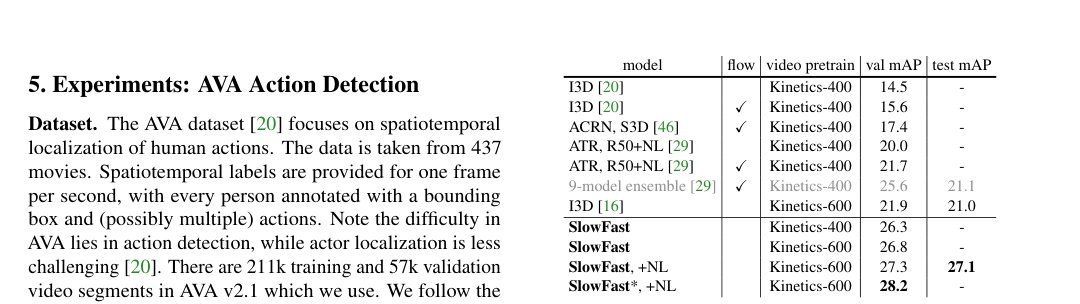
Figure 3: Per-category AP on AVA: a Slow-only baseline (19.0 mAP) vs. its SlowFast counterpart (24.2 mAP). The highlighted categories are the 5 highest absolute increase (black) or 5 highest relative increase with Slow-only AP 1.0 (orange). Categories are sorted by number of examples. Note that the SlowFast instantiation in this ablation is not our best-performing model.
图 3:AVA 上的逐类 AP:仅 Slow 基线(19.0 mAP)对比 对应 SlowFast(24.2 mAP)。高亮类别为绝对提升最大的 5 类(黑),或仅 Slow AP 时相对提升最大的 5 类(橙)。类别按样本数排序。注意该消融中的 SlowFast 实例化并非我们表现最好的模型。
| model | flow | video pretrain | val mAP | test mAP |
|---|---|---|---|---|
| I3D Gu2018 | Kinetics-400 | 14.5 | - | |
| I3D Gu2018 | ✓ | Kinetics-400 | 15.6 | - |
| ACRN, S3D Sun2018 | ✓ | Kinetics-400 | 17.4 | - |
| ATR, R50+NL Jiang2018 | Kinetics-400 | 20.0 | - | |
| ATR, R50+NL Jiang2018 | ✓ | Kinetics-400 | 21.7 | - |
| 9-model ensemble Jiang2018 | ✓ | Kinetics-400 | 25.6 | 21.1 |
| I3D Girdhar2018 | Kinetics-600 | 21.9 | 21.0 | |
| SlowFast | Kinetics-400 | 26.3 | - | |
| SlowFast | Kinetics-600 | 26.8 | - | |
| SlowFast, +NL | Kinetics-600 | 27.3 | 27.1 | |
| SlowFast, +NL* | Kinetics-600 | 28.2 | - |
Table 7: Comparison with the state-of-the-art on AVA v2.1. All our variants are based on 88, R101. Here “*” indicates a version of our method that uses our region proposals for training.
| 模型 | 光流 | 视频预训练 | 验证 mAP | 测试 mAP |
|---|---|---|---|---|
| I3D Gu2018 | Kinetics-400 | 14.5 | - | |
| I3D Gu2018 | ✓ | Kinetics-400 | 15.6 | - |
| ACRN, S3D Sun2018 | ✓ | Kinetics-400 | 17.4 | - |
| ATR, R50+NL Jiang2018 | Kinetics-400 | 20.0 | - | |
| ATR, R50+NL Jiang2018 | ✓ | Kinetics-400 | 21.7 | - |
| 9-model ensemble Jiang2018 | ✓ | Kinetics-400 | 25.6 | 21.1 |
| I3D Girdhar2018 | Kinetics-600 | 21.9 | 21.0 | |
| SlowFast | Kinetics-400 | 26.3 | - | |
| SlowFast | Kinetics-600 | 26.8 | - | |
| SlowFast, +NL | Kinetics-600 | 27.3 | 27.1 | |
| SlowFast, +NL* | Kinetics-600 | 28.2 | - |
表 7:AVA v2.1 上与最好结果的比较。我们全部变体基于 88、R101。这里「*」表示训练时使用我们区域提案的版本。
5.1 Main Results
5.1 主要结果
We compare with previous results on AVA in Table 7. An interesting observation is on the potential benefit of using optical flow (see column ‘flow’ in Table 7). Existing works have observed mild improvements: +1.1 mAP for I3D in Gu2018, and +1.7 mAP for ATR in Jiang2018. In contrast, our baseline improves by the Fast pathway by +5.2 mAP (see Table 9 in our ablation experiments in the next section). Moreover, two-stream methods using optical flow can double the computational cost, whereas our Fast pathway is lightweight.
我们在表 7 与 AVA 上先前结果比较。一个有趣观察是使用光流的潜在收益(见表 7「flow」列)。已有工作观察到温和提升:Gu2018 中 I3D +1.1 mAP,Jiang2018 中 ATR +1.7 mAP。相比之下,我们的基线经 Fast 通路提升 +5.2 mAP(见下一节消融中的表 9)。而且使用光流的双流方法可能使算力翻倍,而我们的 Fast 通路很轻。
As system-level comparisons, our SlowFast model has 26.3 mAP using only Kinetics-400 pre-training. This is 5.6 mAP higher than the previous best number under similar settings (21.7 of ATR Jiang2018, single-model), and 7.3 mAP higher than that using no optical flow (Table 7).
作为系统级比较,我们的 SlowFast 模型仅用 Kinetics-400 预训练即达 26.3 mAP。这比相近设定下先前最好数字(ATR Jiang2018 单模型 21.7)高 5.6 mAP,比不用光流的结果(表 7)高 7.3 mAP。
The work in Girdhar2018 pre-trains on the larger Kinetics-600 and achieves 21.9 mAP. For fair comparison, we observe an improvement from 26.3 mAP to 26.8 mAP for using Kinetics-600. Augmenting SlowFast with NL blocks Wang2018 increases this to 27.3 mAP. We train this model on train+val (and by 1.5 longer) and submit it to the AVA v2.1 test server AVALeaverboard2018. It achieves 27.1 mAP single crop test set accuracy.
Girdhar2018 在更大的 Kinetics-600 上预训练,达到 21.9 mAP。为公平比较,我们观察到改用 Kinetics-600 后从 26.3 mAP 升到 26.8 mAP。给 SlowFast 加上 NL 块 Wang2018 升至 27.3 mAP。我们在 train+val 上训练该模型(并加长 1.5 倍),提交到 AVA v2.1 测试服务器 AVALeaverboard2018,单裁剪测试集达到 27.1 mAP。
By using predicted proposals overlapping with ground-truth boxes by IoU 0.9, in addition to the ground truth boxes, for training we achieve 28.2 mAP single crop validation accuracy, a new state-of-the-art on AVA.
训练时除真实框外,再使用与真实框 IoU 的预测提案,单裁剪验证准确率达到 28.2 mAP,刷新 AVA 最好结果。
| model | flow | video pretrain | val mAP | test mAP |
|---|---|---|---|---|
| SlowFast, 88 | Kinetics-600 | 29.0 | - | |
| SlowFast, 168 | Kinetics-600 | 29.8 | - | |
| SlowFast++, 168 | Kinetics-600 | 30.7 | - | |
| SlowFast++, ensemble | Kinetics-600 | - | 34.3 |
Table 8: SlowFast models on AVA v2.2. Here “++” indicates a version of our method that is tested with multi-scale and horizontal flipping augmentation. The backbone is R-101+NL and region proposals are used for training.
| 模型 | 光流 | 视频预训练 | 验证 mAP | 测试 mAP |
|---|---|---|---|---|
| SlowFast, 88 | Kinetics-600 | 29.0 | - | |
| SlowFast, 168 | Kinetics-600 | 29.8 | - | |
| SlowFast++, 168 | Kinetics-600 | 30.7 | - | |
| SlowFast++, ensemble | Kinetics-600 | - | 34.3 |
表 8:AVA v2.2 上的 SlowFast 模型。这里「++」表示测试时使用多尺度与水平翻转增强的版本。骨干为 R-101+NL,训练使用区域提案。
Using the AVA v2.2 dataset (which provides more consistent annotations) improves this number to 29.0 mAP (Table 8). The longer-term SlowFast, 168 model produces 29.8 mAP and using multiple spatial scales and horizontal flip for testing, this number is increased to 30.7 mAP.
使用标注更一致的 AVA v2.2 数据集,该数字提升到 29.0 mAP(表 8)。更长程的 SlowFast 168 模型达到 29.8 mAP;测试时用多空间尺度与水平翻转,进一步升到 30.7 mAP。
Finally, we create an ensemble of 7 models and submit it to the official test server for the ActivityNet challenge 2019 ActivityNet2019. As shown in Table 8 this entry (SlowFast++, ensemble) achieved 34.3 mAP accuracy on the test set, ranking first in the AVA action detection challenge 2019. Further details on our winning solution are provided in the corresponding technical report Feichtenhofer2019a.
最后,我们集成 7 个模型并提交到 ActivityNet challenge 2019 ActivityNet2019 官方测试服务器。如表 8 所示,该条目(SlowFast++,集成)在测试集达到 34.3 mAP,在 AVA 动作检测挑战 2019 中排名第一。获胜方案的更多细节见对应技术报告 Feichtenhofer2019a。
5.2 Ablation Experiments
5.2 消融实验
Table 9 compares a Slow-only baseline with its SlowFast counterpart, with the per-category AP shown in Fig. 3. Our method improves massively by 5.2 mAP (relative 28%) from 19.0 to 24.2. This is solely contributed by our SlowFast idea.
表 9 比较仅 Slow 基线与对应 SlowFast,逐类 AP 见图 3。我们的方法从 19.0 大幅提升 5.2 mAP(相对 28%)到 24.2。这完全由 SlowFast 思想贡献。
Category-wise (Fig. 3), our SlowFast model improves in 57 out of 60 categories, vs. its Slow-only counterpart. The largest absolute gains are observed for “hand clap" (+27.7 AP), “swim" (+27.4 AP), “run/jog" (+18.8 AP), “dance" (+15.9 AP), and “eat” (+12.5 AP). We also observe large relative increase in “jump/leap”, “hand wave”, “put down”, “throw”, “hit” or “cut”. These are categories where modeling dynamics are of vital importance. The SlowFast model is worse in only 3 categories: “answer phone" (-0.1 AP), “lie/sleep" (-0.2 AP), “shoot" (-0.4 AP), and their decrease is relatively small vs. others’ increase.
按类别看(图 3),相对仅 Slow,我们的 SlowFast 在 60 类中的 57 类上提升。绝对收益最大的是「hand clap」(+27.7 AP)、「swim」(+27.4 AP)、「run/jog」(+18.8 AP)、「dance」(+15.9 AP)与「eat」(+12.5 AP)。我们还在「jump/leap」「hand wave」「put down」「throw」「hit」或「cut」上看到很大相对提升。这些类别里建模动态至关重要。仅在 3 类上变差:「answer phone」(-0.1 AP)、「lie/sleep」(-0.2 AP)、「shoot」(-0.4 AP),且降幅相对其他类的升幅较小。
6 Conclusion
6 结论
The time axis is a special dimension. This paper has investigated an architecture design that contrasts the speed along this axis. It achieves state-of-the-art accuracy for video action classification and detection. We hope that this SlowFast concept will foster further research in video recognition.
时间轴是特殊的一维。本文研究了一种沿该轴对比速度的架构设计。它在视频动作分类与检测上达到当时最好准确率。我们希望 SlowFast 概念能推动视频识别的进一步研究。
| model | mAP | ||
|---|---|---|---|
| Slow-only, R-50 | 416 | - | 19.0 |
| SlowFast, R-50 | 416 | 8 | 24.2 |
Table 9: AVA action detection baselines: Slow-only vs. SlowFast.
| 模型 | mAP | ||
|---|---|---|---|
| 仅 Slow,R-50 | 416 | - | 19.0 |
| SlowFast, R-50 | 416 | 8 | 24.2 |
表 9:AVA 动作检测基线:仅 Slow 对比 SlowFast。
Appendix A Appendix
附录 A 附录
Implementation details.
We study backbones including ResNet-50 and the deeper ResNet-101 He2016, optionally augmented with non-local (NL) blocks Wang2018. For models involving R-101, we use a scale jittering range of [256, 340]. The 168 models are initilaized from the 88 counterparts and trained for half the training epochs to reduce training time. For all models involving NL, we initialize them with the counterparts that are trained without NL, to facilitate convergence. We only use NL on the (fused) Slow features of res4 (instead of res3+res4 Wang2018).
实现细节。
我们研究包括 ResNet-50 与更深的 ResNet-101 He2016 在内的骨干,可选地加上 nonlocal(NL)块 Wang2018。涉及 R-101 的模型使用 [256, 340] 的尺度抖动范围。 168 模型由 88 对应模型初始化,训练 epoch 减半以缩短训练时间。所有含 NL 的模型由不含 NL 的对应模型初始化,以利于收敛。我们只在 res4 的(融合后)Slow 特征上使用 NL(而非 Wang2018 的 res3+res4)。
On Kinetics, we adopt synchronized SGD training in 128 GPUs following the recipe in Goyal2017, and we found its accuracy is as good as typical training in one 8-GPU machine but it scales out well. The mini-batch size is 8 clips per GPU (so the total mini-batch size is 1024). We use the initialization method in He2015. We train with Batch Normalization (BN) Ioffe2015 with BN statistics computed within each 8 clips. We adopt a half-period cosine schedule Loshchilov2016 of learning rate decaying: the learning rate at the -th iteration is , where is the maximum training iterations and the base learning rate is set as 1.6. We also use a linear warm-up strategy Goyal2017 in the first 8k iterations. For Kinetic-400, we train for 256 epochs (60k iterations with a total mini-batch size of 1024, in 240k Kinetics videos) when 4 frames, and 196 epochs when 4 frames: it is sufficient to train shorter when a clip has more frames. We use momentum of 0.9 and weight decay of 10. Dropout Hinton2012b of 0.5 is used before the final classifier layer.
在 Kinetics 上,我们按 Goyal2017 在 128 个 GPU 上做同步 SGD,发现准确率与典型单机 8 GPU 训练一样好,且扩展性良好。每 GPU 小批量 8 个片段(总小批量 1024)。初始化用 He2015。训练使用 Batch Normalization(BN)Ioffe2015,BN 统计在每 8 个片段内计算。学习率衰减采用半周期余弦调度 Loshchilov2016:第 次迭代学习率为 ,其中 为最大训练迭代,基础学习率 设为 1.6。前 8k 次迭代还使用线性热身 Goyal2017。对 Kinetics-400,当 4 帧时训 256 个 epoch(总小批量 1024 时约 6 万次迭代,约 24 万条 Kinetics 视频);当 4 帧时训 196 个 epoch:片段帧数更多时训短一些即可。动量 0.9,权重衰减 。最终分类层前使用 0.5 的 Dropout Hinton2012b。
For Kinetics-600, we extend the training epochs (and schedule) by 2 and set the base learning rate to 0.8.
对 Kinetics-600,我们把训练 epoch(及调度)延长 2 倍,并把基础学习率 设为 0.8。
For Charades, we fine-tune the Kinetics models. A per-class sigmoid output is used to account for the mutli-class nature. We train on a single machine for 24k iterations using a batch size of 16 and a base learning rate of 0.0375 (Kinetics-400 pre-trained) and 0.02 (Kinetics-600 pre-trained) with 10 step-wise decay if the validation error saturates. For inference, we temporally max-pool scores Wang2018.
对 Charades,我们微调 Kinetics 模型。使用按类 sigmoid 输出以适配多标签性质。在单机上训练 2.4 万次迭代,batch 为 16,基础学习率对 Kinetics-400 预训练为 0.0375、对 Kinetics-600 预训练为 0.02,验证误差饱和时按 10 倍阶梯衰减。推理时对分数做时间最大池化 Wang2018。
References
参考文献
(1) ActivityNet-Challenge. http://activity-net.org/challenges/2019/evaluation.html .
(2) E. H. Adelson and J. R. Bergen. Spatiotemporal energy models for the perception of motion. J. Opt. Soc. Am. A , 2(2):284–299, 1985.
(3) J. Carreira, E. Noland, A. Banki-Horvath, C. Hillier, and A. Zisserman. A short note about Kinetics-600. arXiv:1808.01340 , 2018.
(4) J. Carreira, E. Noland, C. Hillier, and A. Zisserman. A short note on the kinetics-700 human action dataset. arXiv preprint arXiv:1907.06987 , 2019.
(5) J. Carreira and A. Zisserman. Quo vadis, action recognition? a new model and the kinetics dataset. In Proc. CVPR , 2017.
(6) N. Dalal, B. Triggs, and C. Schmid. Human detection using oriented histograms of flow and appearance. In Proc. ECCV , 2006.
(7) J. Deng, W. Dong, R. Socher, L.-J. Li, K. Li, and L. Fei-Fei. ImageNet: A large-scale hierarchical image database. In Proc. CVPR , 2009.
(8) A. Derrington and P. Lennie. Spatial and temporal contrast sensitivities of neurones in lateral geniculate nucleus of macaque. The Journal of physiology , 357(1):219–240, 1984.
(9) A. Diba, M. Fayyaz, V. Sharma, M. M. Arzani, R. Yousefzadeh, J. Gall, and L. Van Gool. Spatio-temporal channel correlation networks for action classification. In Proc. ECCV , 2018.
(10) P. Dollár, V. Rabaud, G. Cottrell, and S. Belongie. Behavior recognition via sparse spatio-temporal features. In PETS Workshop, ICCV , 2005.
(11) C. Feichtenhofer, H. Fan, J. Malik, and K. He. SlowFast networks for video recognition in ActivityNet challenge 2019. http://static.googleusercontent.com/media/research.google.com/en//ava/2019/fair_slowfast.pdf , 2019.
(12) C. Feichtenhofer, A. Pinz, and R. Wildes. Spatiotemporal residual networks for video action recognition. In NIPS , 2016.
(13) C. Feichtenhofer, A. Pinz, and A. Zisserman. Convolutional two-stream network fusion for video action recognition. In Proc. CVPR , 2016.
(14) D. J. Felleman and D. C. Van Essen. Distributed hierarchical processing in the primate cerebral cortex. Cerebral cortex (New York, NY: 1991) , 1(1):1–47, 1991.
(15) B. Ghanem, J. C. Niebles, C. Snoek, F. C. Heilbron, H. Alwassel, V. Escorcia, R. Khrisna, S. Buch, and C. D. Dao. The ActivityNet large-scale activity recognition challenge 2018 summary. arXiv:1808.03766 , 2018.
(16) R. Girdhar, J. Carreira, C. Doersch, and A. Zisserman. A better baseline for AVA. arXiv:1807.10066 , 2018.
(17) R. Girshick. Fast R-CNN. In Proc. ICCV , 2015.
(18) R. Girshick, I. Radosavovic, G. Gkioxari, P. Dollár, and K. He. Detectron. https://github.com/facebookresearch/detectron , 2018.
(19) P. Goyal, P. Dollár, R. Girshick, P. Noordhuis, L. Wesolowski, A. Kyrola, A. Tulloch, Y. Jia, and K. He. Accurate, large minibatch SGD: training ImageNet in 1 hour. arXiv:1706.02677 , 2017.
(20) C. Gu, C. Sun, D. A. Ross, C. Vondrick, C. Pantofaru, Y. Li, S. Vijayanarasimhan, G. Toderici, S. Ricco, R. Sukthankar, C. Schmid, and J. Malik. AVA: A video dataset of spatio-temporally localized atomic visual actions. In Proc. CVPR , 2018.
(21) D. He, F. Li, Q. Zhao, X. Long, Y. Fu, and S. Wen. Exploiting spatial-temporal modelling and multi-modal fusion for human action recognition. arXiv:1806.10319 , 2018.
(22) K. He, G. Gkioxari, P. Dollár, and R. Girshick. Mask R-CNN. In Proc. ICCV , 2017.
(23) K. He, X. Zhang, S. Ren, and J. Sun. Delving deep into rectifiers: Surpassing human-level performance on imagenet classification. In Proc. CVPR , 2015.
(24) K. He, X. Zhang, S. Ren, and J. Sun. Deep residual learning for image recognition. In Proc. CVPR , 2016.
(25) G. E. Hinton, N. Srivastava, A. Krizhevsky, I. Sutskever, and R. R. Salakhutdinov. Improving neural networks by preventing co-adaptation of feature detectors. arXiv:1207.0580 , 2012.
(26) J. Huang and D. Mumford. Statistics of natural images and models. In Proc. CVPR , 1999.
(27) D. H. Hubel and T. N. Wrisel. Receptive fields and functional architecture in two non-striate visual areas of the cat. J. Neurophysiol , 28:229–289, 1965.
(28) S. Ioffe and C. Szegedy. Batch normalization: Accelerating deep network training by reducing internal covariate shift. In Proc. ICML , 2015.
(29) J. Jiang, Y. Cao, L. Song, S. Z. Y. Li, Z. Xu, Q. Wu, C. Gan, C. Zhang, and G. Yu. Human centric spatio-temporal action localization. In ActivityNet workshop, CVPR , 2018.
(30) W. Kay, J. Carreira, K. Simonyan, B. Zhang, C. Hillier, S. Vijayanarasimhan, F. Viola, T. Green, T. Back, P. Natsev, et al. The kinetics human action video dataset. arXiv:1705.06950 , 2017.
(31) A. Kläser, M. Marszałek, and C. Schmid. A spatio-temporal descriptor based on 3d-gradients. In Proc. BMVC. , 2008.
(32) A. Krizhevsky, I. Sutskever, and G. E. Hinton. ImageNet classification with deep convolutional neural networks. In NIPS , 2012.
(33) I. Laptev, M. Marszalek, C. Schmid, and B. Rozenfeld. Learning realistic human actions from movies. In Proc. CVPR , 2008.
(34) Leaderboard:ActivityNet-AVA. http://activity-net.org/challenges/2018/evaluation.html .
(35) T.-Y. Lin, P. Dollár, R. Girshick, K. He, B. Hariharan, and S. Belongie. Feature pyramid networks for object detection. In Proc. CVPR , 2017.
(36) T.-Y. Lin, M. Maire, S. Belongie, J. Hays, P. Perona, D. Ramanan, P. Dollár, and C. L. Zitnick. Microsoft coco: Common objects in context. In Proc. ECCV , 2014.
(37) M. Livingstone and D. Hubel. Segregation of form, color, movement, and depth: anatomy, physiology, and perception. Science , 240(4853):740–749, 1988.
(38) I. Loshchilov and F. Hutter. SGDR: Stochastic gradient descent with warm restarts. arXiv:1608.03983 , 2016.
(39) Z. Qiu, T. Yao, and T. Mei. Learning spatio-temporal representation with pseudo-3d residual networks. In Proc. ICCV , 2017.
(40) S. Ren, K. He, R. Girshick, and J. Sun. Faster R-CNN: Towards real-time object detection with region proposal networks. In NIPS , 2015.
(41) D. L. Ruderman. The statistics of natural images. Network: computation in neural systems , 5(4):517–548, 1994.
(42) G. A. Sigurdsson, S. K. Divvala, A. Farhadi, and A. Gupta. Asynchronous temporal fields for action recognition. In CVPR , 2017.
(43) G. A. Sigurdsson, G. Varol, X. Wang, A. Farhadi, I. Laptev, and A. Gupta. Hollywood in homes: Crowdsourcing data collection for activity understanding. In ECCV , 2016.
(44) K. Simonyan and A. Zisserman. Two-stream convolutional networks for action recognition in videos. In NIPS , 2014.
(45) K. Simonyan and A. Zisserman. Very deep convolutional networks for large-scale image recognition. In Proc. ICLR , 2015.
(46) C. Sun, A. Shrivastava, C. Vondrick, K. Murphy, R. Sukthankar, and C. Schmid. Actor-centric relation network. In ECCV , 2018.
(47) C. Szegedy, W. Liu, Y. Jia, P. Sermanet, S. Reed, D. Anguelov, D. Erhan, V. Vanhoucke, and A. Rabinovich. Going deeper with convolutions. In Proc. CVPR , 2015.
(48) G. W. Taylor, R. Fergus, Y. LeCun, and C. Bregler. Convolutional learning of spatio-temporal features. In Proc. ECCV , 2010.
(49) D. Tran, L. Bourdev, R. Fergus, L. Torresani, and M. Paluri. Learning spatiotemporal features with 3D convolutional networks. In Proc. ICCV , 2015.
(50) D. Tran, H. Wang, L. Torresani, J. Ray, Y. LeCun, and M. Paluri. A closer look at spatiotemporal convolutions for action recognition. In Proc. CVPR , 2018.
(51) D. C. Van Essen and J. L. Gallant. Neural mechanisms of form and motion processing in the primate visual system. Neuron , 13(1):1–10, 1994.
(52) G. Varol, I. Laptev, and C. Schmid. Long-term temporal convolutions for action recognition. IEEE PAMI , 2018.
(53) H. Wang and C. Schmid. Action recognition with improved trajectories. In Proc. ICCV , 2013.
(54) L. Wang, W. Li, W. Li, and L. Van Gool. Appearance-and-relation networks for video classification. In Proc. CVPR , 2018.
(55) L. Wang, Y. Xiong, Z. Wang, Y. Qiao, D. Lin, X. Tang, and L. Val Gool. Temporal segment networks: Towards good practices for deep action recognition. In Proc. ECCV , 2016.
(56) X. Wang, R. Girshick, A. Gupta, and K. He. Non-local neural networks. In Proc. CVPR , 2018.
(57) X. Wang and A. Gupta. Videos as space-time region graphs. In ECCV , 2018.
(58) Y. Weiss, E. P. Simoncelli, and E. H. Adelson. Motion illusions as optimal percepts. Nature neuroscience , 5(6):598, 2002.
(59) C.-Y. Wu, M. Zaheer, H. Hu, R. Manmatha, A. J. Smola, and P. Krähenbühl. Compressed video action recognition. In CVPR , 2018.
(60) S. Xie, R. Girshick, P. Dollár, Z. Tu, and K. He. Aggregated residual transformations for deep neural networks. In Proc. CVPR , 2017.
(61) S. Xie, C. Sun, J. Huang, Z. Tu, and K. Murphy. Rethinking spatiotemporal feature learning for video understanding. arXiv:1712.04851 , 2017.
(62) B. Zhou, A. Andonian, A. Oliva, and A. Torralba. Temporal relational reasoning in videos. In ECCV , 2018.
(63) M. Zolfaghari, K. Singh, and T. Brox. ECO: efficient convolutional network for online video understanding. In Proc. ECCV , 2018.