Exploring Simple Siamese Representation Learning

探索简单的孪生表示学习

Xinlei Chen   Kaiming He Facebook AI Research (FAIR)

Abstract

摘要

Siamese networks have become a common structure in various recent models for unsupervised visual representation learning. These models maximize the similarity between two augmentations of one image, subject to certain conditions for avoiding collapsing solutions. In this paper, we report surprising empirical results that simple Siamese networks can learn meaningful representations even using none of the following: (i) negative sample pairs, (ii) large batches, (iii) momentum encoders. Our experiments show that collapsing solutions do exist for the loss and structure, but a stop-gradient operation plays an essential role in preventing collapsing. We provide a hypothesis on the implication of stop-gradient, and further show proof-of-concept experiments verifying it. Our “SimSiam” method achieves competitive results on ImageNet and downstream tasks. We hope this simple baseline will motivate people to rethink the roles of Siamese architectures for unsupervised representation learning. Code will be made available.

孪生网络已成为近期多种无监督视觉表示学习模型中的常见结构。这些模型在避免塌缩解的若干条件下，最大化同一图像两份增强视图之间的相似度。本文报告令人惊讶的经验结果：简单孪生网络即便完全不用以下任一手段仍可学到有意义表示：(i) 负样本对，(ii) 大 batch，(iii) 动量编码器。实验表明损失与结构下塌缩解确实存在，但 stop-gradient 操作在防止塌缩中起关键作用。我们就 stop-gradient 的含义提出假设，并用概念验证实验加以检验。我们的「SimSiam」方法在 ImageNet 与下游任务上取得有竞争力的结果。希望这一简单基线促使人们重新思考孪生架构在无监督表示学习中的角色。代码将公开。

1 Introduction

1 引言

Recently there has been steady progress in un-/self-supervised representation learning, with encouraging results on multiple visual tasks (\eg, [2, 17, 8, 15, 7]). Despite various original motivations, these methods generally involve certain forms of Siamese networks [4]. Siamese networks are weight-sharing neural networks applied on two or more inputs. They are natural tools for comparing (including but not limited to “contrasting”) entities. Recent methods define the inputs as two augmentations of one image, and maximize the similarity subject to different conditions.

近期无/自监督表示学习稳步进展，多项视觉任务上结果令人鼓舞（例如 [2, 17, 8, 15, 7]）。尽管初始动机各异，这些方法通常都涉及某种形式的孪生网络 [4]。孪生网络是作用于两个或多个输入、共享权重的神经网络，是比较（包括但不限于「对比」）实体的自然工具。近期方法把输入定义为同一图像的两份增强，并在不同条件下最大化相似度。

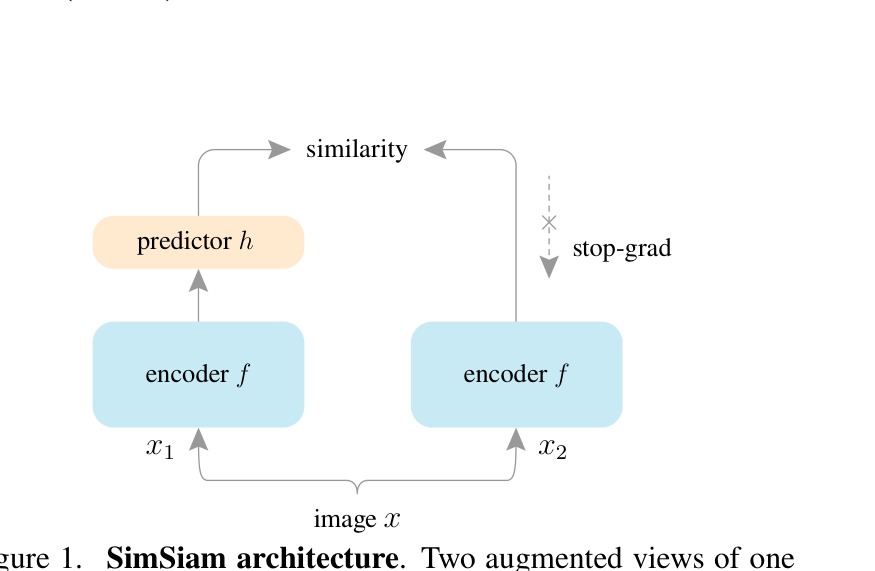
Figure 1: SimSiam architecture. Two augmented views of one image are processed by the same encoder network $f$ (a backbone plus a projection MLP). Then a prediction MLP $h$ is applied on one side, and a stop-gradient operation is applied on the other side. The model maximizes the similarity between both sides. It uses neither negative pairs nor a momentum encoder.

图 1：SimSiam 架构。同一图像的两份增强视图由同一编码器网络 $f$（骨干加投影 MLP）处理。随后一侧接预测 MLP $h$，另一侧施加 stop-gradient。模型最大化两侧相似度。既不用负样本对，也不用动量编码器。

An undesired trivial solution to Siamese networks is all outputs “collapsing” to a constant. There have been several general strategies for preventing Siamese networks from collapsing. Contrastive learning [16], \eg, instantiated in SimCLR [8], repulses different images (negative pairs) while attracting the same image’s two views (positive pairs). The negative pairs preclude constant outputs from the solution space. Clustering [5] is another way of avoiding constant output, and SwAV [7] incorporates online clustering into Siamese networks. Beyond contrastive learning and clustering, BYOL [15] relies only on positive pairs but it does not collapse in case a momentum encoder is used.

孪生网络不受欢迎的平凡解是所有输出「塌缩」成常数。已有若干通用策略防止孪生网络塌缩。对比学习 [16]，例如在 SimCLR [8] 中的实例化，排斥不同图像（负对）同时吸引同一图像的两视图（正对）。负对把常数输出排除出解空间。聚类 [5] 是另一避免常数输出的途径，SwAV [7] 把在线聚类并入孪生网络。在对比学习与聚类之外，BYOL [15] 仅依赖正对，但在使用动量编码器时不塌缩。

In this paper, we report that simple Siamese networks can work surprisingly well with none of the above strategies for preventing collapsing. Our model directly maximizes the similarity of one image’s two views, using neither negative pairs nor a momentum encoder. It works with typical batch sizes and does not rely on large-batch training. We illustrate this “SimSiam” method in Figure 1.

本文报告：简单孪生网络即便完全不用上述防塌缩策略也能出奇地好用。我们的模型直接最大化同一图像两视图的相似度，既不用负对 也不用动量编码器。它在常见 batch 大小下工作，不依赖大 batch 训练。图 1 示意这一「SimSiam」方法。

Thanks to the conceptual simplicity, SimSiam can serve as a hub that relates several existing methods. In a nutshell, our method can be thought of as “BYOL without the momentum encoder”. Unlike BYOL but like SimCLR and SwAV, our method directly shares the weights between the two branches, so it can also be thought of as “SimCLR without negative pairs”, and “SwAV without online clustering”. Interestingly, SimSiam is related to each method by removing one of its core components. Even so, SimSiam does not cause collapsing and can perform competitively.

得益于概念简洁，SimSiam 可作为关联多种已有方法的枢纽。简言之，可视为「去掉动量编码器的 BYOL」。与 BYOL 不同而类似 SimCLR 与 SwAV，我们的方法两支路直接共享权重，因而也可视为「去掉负对的 SimCLR」以及「去掉在线聚类的 SwAV」。有趣的是，SimSiam 与各方法的关系都是去掉其中一个核心组件；即便如此，它仍不塌缩且表现有竞争力。

We empirically show that collapsing solutions do exist, but a stop-gradient operation (Figure 1) is critical to prevent such solutions. The importance of stop-gradient suggests that there should be a different underlying optimization problem that is being solved. We hypothesize that there are implicitly two sets of variables, and SimSiam behaves like alternating between optimizing each set. We provide proof-of-concept experiments to verify this hypothesis.

我们经验上表明塌缩解确实存在，但 stop-gradient 操作（图 1）对防止此类解至关重要。stop-gradient 的重要性暗示实际求解的是另一个底层优化问题。我们假设隐式存在两套变量，SimSiam 表现得像在交替优化每一套。我们提供概念验证实验检验该假设。

Our simple baseline suggests that the Siamese architectures can be an essential reason for the common success of the related methods. Siamese networks can naturally introduce inductive biases for modeling invariance, as by definition “invariance” means that two observations of the same concept should produce the same outputs. Analogous to convolutions [25], which is a successful inductive bias via weight-sharing for modeling translation-invariance, the weight-sharing Siamese networks can model invariance \wrtmore complicated transformations (\eg, augmentations). We hope our exploration will motivate people to rethink the fundamental roles of Siamese architectures for unsupervised representation learning.

这一简单基线表明，孪生架构可能是相关方法共同成功的关键原因。孪生网络可自然引入建模不变性的归纳偏置，因为按定义「不变性」意味着同一概念的两次观测应产生相同输出。类比卷积 [25]——通过权重共享成功建模平移不变性的归纳偏置——权重共享的孪生网络可建模相对更复杂变换（例如增强）的不变性。希望我们的探索促使人们重新思考孪生架构对无监督表示学习的根本作用。

2 Related Work

2 相关工作

Siamese networks.

Siamese networks [4] are general models for comparing entities. Their applications include signature [4] and face [34] verification, tracking [3], one-shot learning [23], and others. In conventional use cases, the inputs to Siamese networks are from different images, and the comparability is determined by supervision.

孪生网络。

孪生网络 [4] 是比较实体的通用模型。应用包括签名 [4] 与人脸 [34] 验证、跟踪 [3]、单样本学习 [23] 等。传统用法中输入来自不同图像，可比性由监督决定。

Contrastive learning.

The core idea of contrastive learning [16] is to attract the positive sample pairs and repulse the negative sample pairs. This methodology has been recently popularized for un-/self-supervised representation learning [36, 30, 20, 37, 21, 2, 35, 17, 29, 8, 9]. Simple and effective instantiations of contrastive learning have been developed using Siamese networks [37, 2, 17, 8, 9].

对比学习。

对比学习 [16] 的核心思想是吸引正样本对、排斥负样本对。该方法近期在无/自监督表示学习中流行 [36, 30, 20, 37, 21, 2, 35, 17, 29, 8, 9]。用孪生网络已发展出简单有效的对比学习实例 [37, 2, 17, 8, 9]。

In practice, contrastive learning methods benefit from a large number of negative samples [36, 35, 17, 8]. These samples can be maintained in a memory bank [36]. In a Siamese network, MoCo [17] maintains a queue of negative samples and turns one branch into a momentum encoder to improve consistency of the queue. SimCLR [8] directly uses negative samples coexisting in the current batch, and it requires a large batch size to work well.

实践中，对比学习受益于大量负样本 [36, 35, 17, 8]。负样本可保存在记忆库中 [36]。在孪生网络中，MoCo [17] 维护负样本队列并把一支变成动量编码器以改善队列一致性。SimCLR [8] 直接使用当前 batch 中共存的负样本，因而需要大 batch 才能表现良好。

Clustering.

Another category of methods for unsupervised representation learning are based on clustering [5, 6, 1, 7]. They alternate between clustering the representations and learning to predict the cluster assignment. SwAV [7] incorporates clustering into a Siamese network, by computing the assignment from one view and predicting it from another view. SwAV performs online clustering under a balanced partition constraint for each batch, which is solved by the Sinkhorn-Knopp transform [10].

聚类。

无监督表示学习的另一类方法基于聚类 [5, 6, 1, 7]。它们在聚类表示与学习预测聚类分配之间交替。SwAV [7] 通过从一视图计算分配、从另一视图预测之，把聚类并入孪生网络。SwAV 在每 batch 的平衡划分约束下做在线聚类，由 Sinkhorn-Knopp 变换 [10] 求解。

While clustering-based methods do not define negative exemplars, the cluster centers can play as negative prototypes. Like contrastive learning, clustering-based methods require either a memory bank [5, 6, 1], large batches [7], or a queue [7] to provide enough samples for clustering.

虽聚类方法不定义负样本范例，聚类中心可扮演负原型。与对比学习类似，聚类方法需要记忆库 [5, 6, 1]、大 batch [7] 或队列 [7] 以提供足够样本。

BYOL.

BYOL [15] directly predicts the output of one view from another view. It is a Siamese network in which one branch is a momentum encoder.[^1] It is hypothesized in [15] that the momentum encoder is important for BYOL to avoid collapsing, and it reports failure results if removing the momentum encoder (0.3% accuracy, Table 5 in [15]).[^2] Our empirical study challenges the necessity of the momentum encoder for preventing collapsing. We discover that the stop-gradient operation is critical. This discovery can be obscured with the usage of a momentum encoder, which is always accompanied with stop-gradient (as it is not updated by its parameters’ gradients). While the moving-average behavior may improve accuracy with an appropriate momentum coefficient, our experiments show that it is not directly related to preventing collapsing.

BYOL。

BYOL [15] 直接由一视图预测另一视图的输出。它是孪生网络，其中一支为动量编码器。[^1] [15] 假设动量编码器对 BYOL 避免塌缩很重要，并报告去掉动量编码器后失败（0.3% 准确率，[15] 表 5）。[^2] 我们的经验研究挑战动量编码器对防塌缩的必要性。我们发现 stop-gradient 操作才是关键。该发现可能被动量编码器的使用掩盖——动量编码器总伴随 stop-gradient（因其不由其参数梯度更新）。虽滑动平均行为可能在合适动量系数下提升准确率，实验表明它与防塌缩无直接关系。

3 Method

3 方法

f: backbone + projection mlp

h: prediction mlp

for x in loader: # load a minibatch x with n samples
x1, x2 = aug(x), aug(x) # random augmentation
z1, z2 = f(x1), f(x2) # projections, n-by-d
p1, p2 = h(z1), h(z2) # predictions, n-by-d

L = D(p1, z2)/2 + D(p2, z1)/2 # loss

L.backward() # back-propagate
update(f, h) # SGD update

def D(p, z): # negative cosine similarity
z = z.detach() # stop gradient

p = normalize(p, dim=1) # l2-normalize
z = normalize(z, dim=1) # l2-normalize
return -(p*z).sum(dim=1).mean()

Algorithm 1 SimSiam Pseudocode, PyTorch-like

f：骨干 + 投影 mlp

h：预测 mlp

for x in loader: # 加载含 n 个样本的小批量 x
x1, x2 = aug(x), aug(x) # 随机增强
z1, z2 = f(x1), f(x2) # 投影，n-by-d
p1, p2 = h(z1), h(z2) # 预测，n-by-d

L = D(p1, z2)/2 + D(p2, z1)/2 # 损失

L.backward() # 反向传播
update(f, h) # SGD 更新

def D(p, z): # 负余弦相似度
z = z.detach() # 停止梯度

p = normalize(p, dim=1) # l2 归一化
z = normalize(z, dim=1) # l2 归一化
return -(p*z).sum(dim=1).mean()

算法 1 SimSiam 伪代码，类 PyTorch

	acc. (%)
w/ stop-grad	67.7$\pm$0.1
w/o stop-grad	0.1

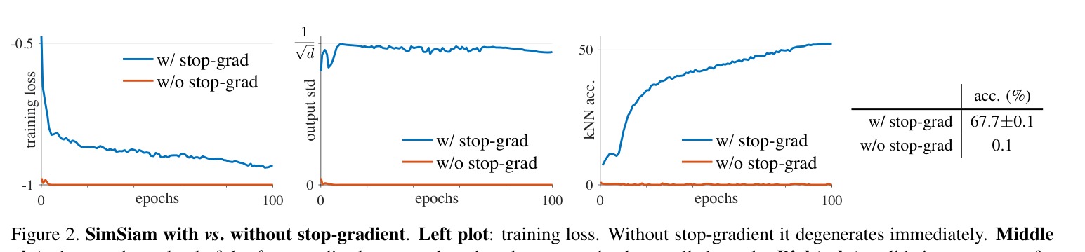
Figure 2: SimSiam with \vswithout stop-gradient. Left plot: training loss. Without stop-gradient it degenerates immediately. Middle plot: the per-channel std of the $\ell_{2}$-normalized output, plotted as the averaged std over all channels. Right plot: validation accuracy of a kNN classifier [36] as a monitor of progress. Table: ImageNet linear evaluation (“w/ stop-grad” is mean$\pm$std over 5 trials).

	acc. (%)
w/ stop-grad	67.7$\pm$0.1
w/o stop-grad	0.1

图 2：SimSiam 有/无 stop-gradient。左图：训练损失。无 stop-gradient 时立即退化。中图：对 $\ell_{2}$ 归一化输出的逐通道标准差，画为所有通道平均 std。右图：kNN 分类器 [36] 验证准确率，用作进度监视。表：ImageNet 线性评估（「w/ stop-grad」为 5 次试验的均值$\pm$标准差）。

Our architecture (Figure 1) takes as input two randomly augmented views $x_{1}$ and $x_{2}$ from an image $x$. The two views are processed by an encoder network $f$ consisting of a backbone (\eg, ResNet [19]) and a projection MLP head [8]. The encoder $f$ shares weights between the two views. A prediction MLP head [15], denoted as $h$, transforms the output of one view and matches it to the other view. Denoting the two output vectors as ${p}_{1}\!\triangleq\!h(f(x_{1}))$ and ${z}_{2}\!\triangleq\!f(x_{2})$, we minimize their negative cosine similarity:

我们的架构（图 1）以图像 $x$ 的两份随机增强视图 $x_{1}$、$x_{2}$ 为输入。两视图由编码器网络 $f$ 处理，$f$ 由骨干（例如 ResNet [19]）与投影 MLP 头 [8] 组成。编码器 $f$ 在两视图间共享权重。预测 MLP 头 [15] 记为 $h$，变换一视图的输出并与另一视图匹配。记两输出向量为 ${p}_{1}\!\triangleq\!h(f(x_{1}))$ 与 ${z}_{2}\!\triangleq\!f(x_{2})$，最小化其负余弦相似度：

$$\mathcal{D}({p}_{1},{z}_{2})=-\frac{{p}_{1}}{\left\lVert{{p}_{1}}\right\rVert_{2}}{\cdot}\frac{{z}_{2}}{\left\lVert{{z}_{2}}\right\rVert_{2}}, \tag{1}$$

where ${\left\lVert{\cdot}\right\rVert_{2}}$ is $\ell_{2}$-norm. This is equivalent to the mean squared error of $\ell_{2}$-normalized vectors [15], up to a scale of 2. Following [15], we define a symmetrized loss as:

其中 ${\left\lVert{\cdot}\right\rVert_{2}}$ 为 $\ell_{2}$ 范数。这等价于 $\ell_{2}$ 归一化向量的均方误差 [15]，相差一个 2 的尺度。沿用 [15]，定义对称损失为：

$$\mathcal{L}=\frac{1}{2}\mathcal{D}({p}_{1},{z}_{2})+\frac{1}{2}\mathcal{D}({p}_{2},{z}_{1}). \tag{2}$$

This is defined for each image, and the total loss is averaged over all images. Its minimum possible value is $-1$.

该损失对每张图像定义，总损失对所有图像取平均。其可能最小值为 $-1$。

An important component for our method to work is a stop-gradient (stopgrad) operation (Figure 1). We implement it by modifying (1) as:

方法能工作的一个重要组件是 stop-gradient（stopgrad）操作（图 1）。我们通过把 (1) 改成下式实现：

$$\mathcal{D}({p}_{1},\texttt{stopgrad}({z}_{2})). \tag{3}$$

This means that ${z}_{2}$ is treated as a constant in this term. Similarly, the form in (2) is implemented as:

这意味着在该项中把 ${z}_{2}$ 当作常数。类似地，(2) 的形式实现为：

$$\mathcal{L}{=}\frac{1}{2}\mathcal{D}({p}_{1},\texttt{stopgrad}({z}_{2})){+}\frac{1}{2}\mathcal{D}({p}_{2},\texttt{stopgrad}({z}_{1})). \tag{4}$$

Here the encoder on $x_{2}$ receives no gradient from ${z}_{2}$ in the first term, but it receives gradients from ${p}_{2}$ in the second term (and vice versa for $x_{1}$).

此处 $x_{2}$ 上的编码器在第一项中不从 ${z}_{2}$ 接收梯度，但在第二项中从 ${p}_{2}$ 接收梯度（$x_{1}$ 反之亦然）。

The pseudo-code of SimSiam is in Algorithm 1.

SimSiam 的伪代码见算法 1。

Baseline settings.

Unless specified, our explorations use the following settings for unsupervised pre-training:

基线设定。

除非另有说明，无监督预训练探索使用以下设定：

• • Optimizer. We use SGD for pre-training. Our method does not require a large-batch optimizer such as LARS [38] (unlike [8, 15, 7]). We use a learning rate of $lr{\times}$BatchSize${/}256$ (linear scaling [14]), with a base $lr\!=\!0.05$. The learning rate has a cosine decay schedule [27, 8]. The weight decay is $0.0001$ and the SGD momentum is $0.9$. The batch size is 512 by default, which is friendly to typical 8-GPU implementations. Other batch sizes also work well (Sec. 4.3). We use batch normalization (BN) [22] synchronized across devices, following [8, 15, 7].

• • 优化器。预训练使用 SGD。我们的方法不需要 LARS [38] 一类大 batch 优化器（不同于 [8, 15, 7]）。学习率为 $lr{\times}$BatchSize${/}256$（线性缩放 [14]），基础 $lr\!=\!0.05$。学习率采用余弦衰减日程 [27, 8]。权重衰减 $0.0001$，SGD 动量 $0.9$。默认 batch 大小 512，对常见 8 GPU 实现友好。其他 batch 大小也表现良好（第 4.3 节）。我们跨设备同步批归一化（BN）[22]，沿用 [8, 15, 7]。

• • Projection MLP. The projection MLP (in $f$) has BN applied to each fully-connected (fc) layer, including its output fc. Its output fc has no ReLU. The hidden fc is $2048$-d. This MLP has 3 layers.

• • 投影 MLP。投影 MLP（在 $f$ 中）对每个全连接（fc）层施加 BN，包括输出 fc。输出 fc 无 ReLU。隐层 fc 为 $2048$ 维。该 MLP 共 3 层。

• • Prediction MLP. The prediction MLP ($h$) has BN applied to its hidden fc layers. Its output fc does not have BN (ablation in Sec. 4.4) or ReLU. This MLP has 2 layers. The dimension of $h$’s input and output (${z}$ and ${p}$) is $d\!=\!2048$, and $h$’s hidden layer’s dimension is $512$, making $h$ a bottleneck structure (ablation in supplement).

• • 预测 MLP。预测 MLP（$h$）对隐层 fc 施加 BN。输出 fc 无 BN（第 4.4 节消融）也无 ReLU。该 MLP 共 2 层。$h$ 的输入与输出（${z}$ 与 ${p}$）维度为 $d\!=\!2048$，$h$ 隐层维度为 $512$，使 $h$ 呈瓶颈结构（附录消融）。

We use ResNet-50 [19] as the default backbone. Other implementation details are in supplement. We perform 100-epoch pre-training in ablation experiments.

默认骨干为 ResNet-50 [19]。其他实现细节见附录。消融实验做 100 epoch 预训练。

Experimental setup.

We do unsupervised pre-training on the 1000-class ImageNet training set [11] without using labels. The quality of the pre-trained representations is evaluated by training a supervised linear classifier on frozen representations in the training set, and then testing it in the validation set, which is a common protocol. The implementation details of linear classification are in supplement.

实验设置。

我们在不含标签的 1000 类 ImageNet 训练集 [11] 上做无监督预训练。预训练表示质量通过在训练集冻结表示上训练有监督线性分类器、再在验证集上测试来评估，这是常用协议。线性分类实现细节见附录。

4 Empirical Study

4 经验研究

In this section we empirically study the SimSiam behaviors. We pay special attention to what may contribute to the model’s non-collapsing solutions.

本节经验研究 SimSiam 行为，特别关注什么可能促成模型的非塌缩解。

4.1 Stop-gradient

Figure 2 presents a comparison on “with \vswithout stop-gradient”. The architectures and all hyper-parameters are kept unchanged, and stop-gradient is the only difference.

图 2 给出「有 \vs 无 stop-gradient」的比较。架构与全部超参数保持不变，唯一差别是 stop-gradient。

Figure 2 (left) shows the training loss. Without stop-gradient, the optimizer quickly finds a degenerated solution and reaches the minimum possible loss of $-1$. To show that the degeneration is caused by collapsing, we study the standard deviation (std) of the $\ell_{2}$-normalized output ${{z}}/{\left\lVert{{z}}\right\rVert_{2}}$. If the outputs collapse to a constant vector, their std over all samples should be zero for each channel. This can be observed from the red curve in Figure 2 (middle).

图 2（左）给出训练损失。没有 stop-gradient 时，优化器迅速找到退化解并达到可能的最小损失 $-1$。为说明退化由塌缩引起，我们研究 $\ell_{2}$ 归一化输出 ${{z}}/{\left\lVert{{z}}\right\rVert_{2}}$ 的标准差（std）。若输出塌缩为常向量，则对每个通道、对所有样本的 std 应为零。这可从图 2（中）红曲线观察到。

As a comparison, if the output ${z}$ has a zero-mean isotropic Gaussian distribution, we can show that the std of ${{z}}/{\left\lVert{{z}}\right\rVert_{2}}$ is $\frac{1}{\sqrt{d}}$.[^3] The blue curve in Figure 2 (middle) shows that with stop-gradient, the std value is near $\frac{1}{\sqrt{d}}$. This indicates that the outputs do not collapse, and they are scattered on the unit hypersphere.

作为对照，若输出 ${z}$ 为零均值各向同性高斯分布，可证 ${{z}}/{\left\lVert{{z}}\right\rVert_{2}}$ 的 std 为 $\frac{1}{\sqrt{d}}$。[^3] 图 2（中）蓝曲线显示：有 stop-gradient 时，std 值接近 $\frac{1}{\sqrt{d}}$。这表明输出未塌缩，并散布在单位超球面上。

Figure 2 (right) plots the validation accuracy of a k-nearest-neighbor (kNN) classifier [36]. This kNN classifier can serve as a monitor of the progress. With stop-gradient, the kNN monitor shows a steadily improving accuracy.

图 2（右）画出 k 近邻（kNN）分类器 [36] 的验证准确率。该 kNN 分类器可用作进度监视。有 stop-gradient 时，kNN 监视器显示准确率稳步提升。

The linear evaluation result is in the table in Figure 2. SimSiam achieves a nontrivial accuracy of 67.7%. This result is reasonably stable as shown by the std of 5 trials. Solely removing stop-gradient, the accuracy becomes 0.1%, which is the chance-level guess in ImageNet.

线性评估结果见图 2 中的表。SimSiam 达到非平凡准确率 67.7%。5 次试验的标准差表明该结果相当稳定。仅去掉 stop-gradient，准确率变为 0.1%，即 ImageNet 上的随机猜测水平。

Discussion.

Our experiments show that there exist collapsing solutions. The collapse can be observed by the minimum possible loss and the constant outputs.[^4] The existence of the collapsing solutions implies that it is insufficient for our method to prevent collapsing solely by the architecture designs (\eg, predictor, BN, $\ell_{2}$-norm). In our comparison, all these architecture designs are kept unchanged, but they do not prevent collapsing if stop-gradient is removed.

讨论。

实验表明存在塌缩解。塌缩可由可能的最小损失与常数输出观察到。[^4] 塌缩解的存在意味着：仅靠架构设计（例如预测器、BN、$\ell_{2}$ 范数）不足以防止我们的方法塌缩。在比较中这些架构设计均保持不变，但去掉 stop-gradient 后它们并不能防止塌缩。

The introduction of stop-gradient implies that there should be another optimization problem that is being solved underlying. We propose a hypothesis in Sec. 5.

引入 stop-gradient 意味着背后应有另一个正在求解的优化问题。我们在第 5 节提出假设。

4.2 Predictor

4.2 预测器

	pred. MLP $h$	acc. (%)
baseline	$lr$ with cosine decay	67.7
(a)	no pred. MLP	0.1
(b)	fixed random init.	1.5
(c)	$lr$ not decayed	68.1

Table 1: Effect of prediction MLP (ImageNet linear evaluation accuracy with 100-epoch pre-training). In all these variants, we use the same schedule for the encoder $f$ ($lr$ with cosine decay).

	pred. MLP $h$	acc. (%)
baseline	$lr$ with cosine decay	67.7
(a)	no pred. MLP	0.1
(b)	fixed random init.	1.5
(c)	$lr$ not decayed	68.1

表 1：预测 MLP 的影响（100 epoch 预训练的 ImageNet 线性评估准确率）。所有变体中编码器 $f$ 使用同一日程（带余弦衰减的 $lr$）。

In Table 1 we study the predictor MLP’s effect.

表 1 研究预测 MLP 的作用。

The model does not work if removing $h$ (Table 1a), \ie, $h$ is the identity mapping. Actually, this observation can be expected if the symmetric loss (4) is used. Now the loss is $\frac{1}{2}\mathcal{D}({z}_{1},\texttt{stopgrad}({z}_{2}))$ ${+}$ $\frac{1}{2}\mathcal{D}({z}_{2},\texttt{stopgrad}({z}_{1}))$. Its gradient has the same direction as the gradient of $\mathcal{D}({z}_{1},{z}_{2})$, with the magnitude scaled by $1/2$. In this case, using stop-gradient is equivalent to removing stop-gradient and scaling the loss by 1/2. Collapsing is observed (Table 1a).

去掉 $h$（表 1a）时模型不工作，即 $h$ 为恒等映射。若使用对称损失 (4)，该观察其实可预期。此时损失为 $\frac{1}{2}\mathcal{D}({z}_{1},\texttt{stopgrad}({z}_{2}))$ ${+}$ $\frac{1}{2}\mathcal{D}({z}_{2},\texttt{stopgrad}({z}_{1}))$。其梯度方向与 $\mathcal{D}({z}_{1},{z}_{2})$ 的梯度相同，幅度缩放 $1/2$。此时使用 stop-gradient 等价于去掉 stop-gradient 并把损失乘 $1/2$。观察到塌缩（表 1a）。

We note that this derivation on the gradient direction is valid only for the symmetrized loss. But we have observed that the asymmetric variant (3) also fails if removing $h$, while it can work if $h$ is kept (Sec. 4.6). These experiments suggest that $h$ is helpful for our model.

注意该梯度方向推导仅对对称损失成立。但我们观察到非对称变体 (3) 在去掉 $h$ 时也失败，而保留 $h$ 时可工作（第 4.6 节）。这些实验表明 $h$ 对我们的模型有帮助。

If $h$ is fixed as random initialization, our model does not work either (Table 1b). However, this failure is not about collapsing. The training does not converge, and the loss remains high. The predictor $h$ should be trained to adapt to the representations.

若 $h$ 固定为随机初始化，模型也不工作（表 1b）。但该失败不是塌缩：训练不收敛，损失保持很高。预测器 $h$ 应训练以适配表示。

We also find that $h$ with a constant $lr$ (without decay) can work well and produce even better results than the baseline (Table 1c). A possible explanation is that $h$ should adapt to the latest representations, so it is not necessary to force it converge (by reducing $lr$) before the representations are sufficiently trained. In many variants of our model, we have observed that $h$ with a constant $lr$ provides slightly better results. We use this form in the following subsections.

我们还发现恒定 $lr$（不衰减）的 $h$ 可良好工作，甚至比基线更好（表 1c）。一种可能解释是 $h$ 应适配最新表示，因此不必在表示充分训练前强迫它收敛（通过降低 $lr$）。在许多变体中，恒定 $lr$ 的 $h$ 略优。后续小节采用该形式。

4.3 Batch Size

4.3 Batch 大小

batch size	64	128	256	512	1024	2048	4096
acc. (%)	66.1	67.3	68.1	68.1	68.0	67.9	64.0

Table 2: Effect of batch sizes (ImageNet linear evaluation accuracy with 100-epoch pre-training).

batch size	64	128	256	512	1024	2048	4096
acc. (%)	66.1	67.3	68.1	68.1	68.0	67.9	64.0

表 2：Batch 大小的影响（100 epoch 预训练的 ImageNet 线性评估准确率）。

Table 2 reports the results with a batch size from 64 to 4096. When the batch size changes, we use the same linear scaling rule ($lr$$\times$BatchSize/256) [14] with base $lr\!=\!0.05$. We use 10 epochs of warm-up [14] for batch sizes $\geq\!$ 1024. Note that we keep using the same SGD optimizer (rather than LARS [38]) for all batch sizes studied.

表 2 报告 batch 从 64 到 4096 的结果。改变 batch 时使用同一线性缩放规则（$lr$$imes$BatchSize/256）[14]，基础 $lr\!=\!0.05$。对 batch $\geq\!$ 1024 使用 10 epoch warm-up [14]。注意所有研究的 batch 大小都继续使用同一 SGD 优化器（而非 LARS [38]）。

Our method works reasonably well over this wide range of batch sizes. Even a batch size of 128 or 64 performs decently, with a drop of 0.8% or 2.0% in accuracy. The results are similarly good when the batch size is from 256 to 2048, and the differences are at the level of random variations.

在这一宽泛 batch 范围内方法表现合理。即便 128 或 64 的 batch 也尚可，准确率分别掉 0.8% 或 2.0%。batch 从 256 到 2048 结果相近，差异处于随机波动水平。

This behavior of SimSiam is noticeably different from SimCLR [8] and SwAV [7]. All three methods are Siamese networks with direct weight-sharing, but SimCLR and SwAV both require a large batch (\eg, 4096) to work well.

SimSiam 的这一行为与 SimCLR [8]、SwAV [7] 明显不同。三者都是直接权重共享的孪生网络，但 SimCLR 与 SwAV 都需要大 batch（例如 4096）才能表现良好。

We also note that the standard SGD optimizer does not work well when the batch is too large (even in supervised learning [14, 38]), and our result is lower with a 4096 batch. We expect a specialized optimizer (\eg, LARS [38]) will help in this case. However, our results show that a specialized optimizer is not necessary for preventing collapsing.

我们也注意到标准 SGD 在 batch 过大时表现不佳（即便在监督学习中 [14, 38]），4096 batch 下我们的结果偏低。预期专用优化器（例如 LARS [38]）对此会有帮助。但结果表明专用优化器对防塌缩并非必要。

4.4 Batch Normalization

4.4 批归一化

		proj. MLP’s BN	pred. MLP’s BN
case	hidden	output	hidden	output	acc. (%)
(a)	none	-	-	-	-	34.6
(b)	hidden-only	✓	-	✓	-	67.4
(c)	default	✓	✓	✓	-	68.1
(d)	all	✓	✓	✓	✓	unstable

Table 3: Effect of batch normalization on MLP heads (ImageNet linear evaluation accuracy with 100-epoch pre-training).

		proj. MLP’s BN	pred. MLP’s BN
case	hidden	output	hidden	output	acc. (%)
(a)	none	-	-	-	-	34.6
(b)	hidden-only	✓	-	✓	-	67.4
(c)	default	✓	✓	✓	-	68.1
(d)	all	✓	✓	✓	✓	unstable

表 3：MLP 头上批归一化的影响（100 epoch 预训练的 ImageNet 线性评估准确率）。

Table 3 compares the configurations of BN on the MLP heads. In Table 3a we remove all BN layers in the MLP heads (10-epoch warmup [14] is used specifically for this entry). This variant does not cause collapse, although the accuracy is low (34.6%). The low accuracy is likely because of optimization difficulty. Adding BN to the hidden layers (Table 3b) increases accuracy to 67.4%.

表 3 比较 MLP 头上 BN 的配置。表 3a 去掉 MLP 头中所有 BN 层（该条目专门使用 10 epoch warm-up [14]）。该变体不导致塌缩，但准确率偏低（34.6%）。低准确率很可能来自优化困难。对隐层加 BN（表 3b）把准确率提到 67.4%。

Further adding BN to the output of the projection MLP (\ie, the output of $f$) boosts accuracy to 68.1% (Table 3c), which is our default configuration. In this entry, we also find that the learnable affine transformation (scale and offset [22]) in $f$’s output BN is not necessary, and disabling it leads to a comparable accuracy of 68.2%.

进一步对投影 MLP 的输出（即 $f$ 的输出）加 BN，准确率升至 68.1%（表 3c），这是我们的默认配置。该条目中我们还发现 $f$ 输出 BN 中的可学习仿射变换（尺度与偏移 [22]）并非必要，关掉后准确率仍可比（68.2%）。

Adding BN to the output of the prediction MLP $h$ does not work well (Table 3d). We find that this is not about collapsing. The training is unstable and the loss oscillates.

对预测 MLP $h$ 的输出加 BN 效果不佳（表 3d）。我们发现这不是塌缩问题：训练不稳定，损失振荡。

In summary, we observe that BN is helpful for optimization when used appropriately, which is similar to BN’s behavior in other supervised learning scenarios. But we have seen no evidence that BN helps to prevent collapsing: actually, the comparison in Sec. 4.1 (Figure 2) has exactly the same BN configuration for both entries, but the model collapses if stop-gradient is not used.

总之，我们观察到在恰当使用时 BN 有助于优化，这与 BN 在其他监督学习场景中的行为类似。但没有证据表明 BN 有助于防塌缩：实际上第 4.1 节（图 2）的比较中两条目 BN 配置完全相同，但不用 stop-gradient 时模型仍塌缩。

4.5 Similarity Function

4.5 相似度函数

Besides the cosine similarity function (1), our method also works with cross-entropy similarity. We modify $\mathcal{D}$ as: $\mathcal{D}({p}_{1},{z}_{2})\!=\!{-}\texttt{softmax}({{z}_{2}}){\cdot}\log\texttt{softmax}({{p}_{1}})$. Here the softmax function is along the channel dimension. The output of softmax can be thought of as the probabilities of belonging to each of $d$ pseudo-categories.

除余弦相似度函数 (1) 外，方法也可用交叉熵相似度。把 $\mathcal{D}$ 改为：$\mathcal{D}({p}_{1},{z}_{2})\!=\!{-}\texttt{softmax}({{z}_{2}}){\cdot}\log\texttt{softmax}({{p}_{1}})$。此处 softmax 沿通道维。softmax 输出可视为属于 $d$ 个伪类别各自的概率。

We simply replace the cosine similarity with the cross-entropy similarity, and symmetrize it using (4). All hyper-parameters and architectures are unchanged, though they may be suboptimal for this variant. Here is the comparison:

我们简单用交叉熵相似度替换余弦相似度，并用 (4) 对称化。全部超参数与架构不变，尽管对该变体可能并非最优。比较如下：

The cross-entropy variant can converge to a reasonable result without collapsing. This suggests that the collapsing prevention behavior is not just about the cosine similarity.

交叉熵变体可收敛到合理结果且不塌缩。这表明防塌缩行为不只关乎余弦相似度。

This variant helps to set up a connection to SwAV [7], which we discuss in Sec. 6.2.

该变体有助于建立与 SwAV [7] 的联系，第 6.2 节讨论。

4.6 Symmetrization

4.6 对称化

Thus far our experiments have been based on the symmetrized loss (4). We observe that SimSiam’s behavior of preventing collapsing does not depend on symmetrization. We compare with the asymmetric variant (3) as follows:

至此实验均基于对称损失 (4)。我们观察到 SimSiam 的防塌缩行为并不依赖对称化。与非对称变体 (3) 比较如下：

The asymmetric variant achieves reasonable results. Symmetrization is helpful for boosting accuracy, but it is not related to collapse prevention. Symmetrization makes one more prediction for each image, and we may roughly compensate for this by sampling two pairs for each image in the asymmetric version (“2$\times$”). It makes the gap smaller.

非对称变体取得合理结果。对称化有助于提升准确率，但与防塌缩无关。对称化使每张图像多一次预测；非对称版本中对每张图像采样两对（「2$\times$」）可大致补偿，差距随之缩小。

4.7 Summary

4.7 小结

We have empirically shown that in a variety of settings, SimSiam can produce meaningful results without collapsing. The optimizer (batch size), batch normalization, similarity function, and symmetrization may affect accuracy, but we have seen no evidence that they are related to collapse prevention. It is mainly the stop-gradient operation that plays an essential role.

我们经验表明，在多种设定下 SimSiam 都能产生有意义结果而不塌缩。优化器（batch 大小）、批归一化、相似度函数与对称化可能影响准确率，但未见证据表明它们与防塌缩相关。主要是 stop-gradient 操作起关键作用。

5 Hypothesis

5 假设

We discuss a hypothesis on what is implicitly optimized by SimSiam, with proof-of-concept experiments provided.

我们就 SimSiam 隐式优化什么提出假设，并给出概念验证实验。

5.1 Formulation

5.1 形式化

Our hypothesis is that SimSiam is an implementation of an Expectation-Maximization (EM) like algorithm. It implicitly involves two sets of variables, and solves two underlying sub-problems. The presence of stop-gradient is the consequence of introducing the extra set of variables.

我们的假设是：SimSiam 是一种类期望最大化（EM）算法的实现。它隐式涉及两套变量，并求解两个底层子问题。stop-gradient 的出现是引入额外变量集的结果。

We consider a loss function of the following form:

我们考虑如下形式的损失函数：

$$\mathcal{L}(\theta,\eta)=\mathbb{E}_{x,\mathcal{T}}\Big[\big\|\mathcal{F}_{\theta}(\mathcal{T}(x))-\eta_{x}\big\|_{2}^{2}\Big]. \tag{5}$$

$\mathcal{F}$ is a network parameterized by $\theta$. $\mathcal{T}$ is the augmentation. $x$ is an image. The expectation $\mathbb{E}[\cdot]$ is over the distribution of images and augmentations. For the ease of analysis, here we use the mean squared error $\|\cdot\|^{2}_{2}$, which is equivalent to the cosine similarity if the vectors are $\ell_{2}$-normalized. We do not consider the predictor yet and will discuss it later.

$\mathcal{F}$ 是参数为 $\theta$ 的网络。$\mathcal{T}$ 是增强。$x$ 是图像。期望 $\mathbb{E}[\cdot]$ 对图像与增强的分布取。为便于分析，此处用均方误差 $\|\cdot\|^{2}_{2}$，在向量经 $\ell_{2}$ 归一化时等价于余弦相似度。暂不考虑预测器，稍后讨论。

In (5), we have introduced another set of variables which we denote as $\eta$. The size of $\eta$ is proportional to the number of images. Intuitively, $\eta_{x}$ is the representation of the image $x$, and the subscript x means using the image index to access a sub-vector of $\eta$. $\eta$ is not necessarily the output of a network; it is the argument of an optimization problem.

在 (5) 中我们引入了另一套变量，记为 $\eta$。$\eta$ 的规模与图像数成正比。直观上，$\eta_{x}$ 是图像 $x$ 的表示，下标 x 表示用图像索引访问 $\eta$ 的子向量。$\eta$ 不一定是网络输出；它是优化问题的自变量。

With this formulation, we consider solving:

在此形式下，我们考虑求解：

$$\min_{\theta,\eta}\mathcal{L}(\theta,\eta). \tag{6}$$

Here the problem is \wrtboth $\theta$ and $\eta$. This formulation is analogous to k-means clustering [28]. The variable $\theta$ is analogous to the clustering centers: it is the learnable parameters of an encoder. The variable $\eta_{x}$ is analogous to the assignment vector of the sample $x$ (a one-hot vector in k-means): it is the representation of $x$.

此处问题同时关于 $\theta$ 与 $\eta$。该形式类比 k-means 聚类 [28]。变量 $\theta$ 类比聚类中心：是编码器的可学习参数。变量 $\eta_{x}$ 类比样本 $x$ 的分配向量（k-means 中为一热向量）：是 $x$ 的表示。

Also analogous to k-means, the problem in (6) can be solved by an alternating algorithm, fixing one set of variables and solving for the other set. Formally, we can alternate between solving these two subproblems:

同样类比 k-means，(6) 中的问题可用交替算法求解：固定一套变量求解另一套。形式地，可交替求解这两个子问题：

$$\displaystyle\theta^{t} \\ \displaystyle\leftarrow \\ \displaystyle\arg\min_{\theta}\penalty\ \mathcal{L}(\theta,\eta^{t{-}1}) \\ \displaystyle\eta^{t} \\ \displaystyle\leftarrow \\ \displaystyle\arg\min_{\eta}\penalty\ \mathcal{L}(\theta^{t},\eta) \tag{7}$$

Here $t$ is the index of alternation and “$\leftarrow$” means assigning.

此处 $t$ 是交替索引，「$\leftarrow$」表示赋值。

Solving for $\theta$.

One can use SGD to solve the sub-problem (7). The stop-gradient operation is a natural consequence, because the gradient does not back-propagate to $\eta^{t-1}$ which is a constant in this subproblem.

求解 $\theta$。

可用 SGD 求解子问题 (7)。stop-gradient 操作是自然结果，因为梯度不回传到该子问题中为常数的 $\eta^{t-1}$。

Solving for $\eta$.

The sub-problem (8) can be solved independently for each $\eta_{x}$. Now the problem is to minimize: $\mathbb{E}_{\mathcal{T}}\Big[\|\mathcal{F}_{\theta^{t}}(\mathcal{T}(x))-\eta_{x}\|^{2}_{2}\Big]$ for each image $x$, noting that the expectation is over the distribution of augmentation $\mathcal{T}$. Due to the mean squared error,[^5] it is easy to solve it by:

求解 $\eta$。

子问题 (8) 可对每个 $\eta_{x}$ 独立求解。此时问题是对每张图像 $x$ 最小化：$\mathbb{E}_{\mathcal{T}}\Big[\|\mathcal{F}_{\theta^{t}}(\mathcal{T}(x))-\eta_{x}\|^{2}_{2}\Big]$，注意期望对增强 $\mathcal{T}$ 的分布取。由于均方误差，[^5] 易得解：

$$\eta^{t}_{x}\leftarrow\mathbb{E}_{\mathcal{T}}\Big[\mathcal{F}_{\theta^{t}}(\mathcal{T}(x))\Big]. \tag{9}$$

This indicates that $\eta_{x}$ is assigned with the average representation of $x$ over the distribution of augmentation.

这表明把 $\eta_{x}$ 赋值为 $x$ 在增强分布上的平均表示。

One-step alternation.

SimSiam can be approximated by one-step alternation between (7) and (8). First, we approximate (9) by sampling the augmentation only once, denoted as $\mathcal{T}^{\prime}$, and ignoring $\mathbb{E}_{\mathcal{T}}[\cdot]$:

一步交替。

SimSiam 可用 (7) 与 (8) 之间的一步交替来近似。首先，仅采样增强一次（记为 $\mathcal{T}^{\prime}$）并忽略 $\mathbb{E}_{\mathcal{T}}[\cdot]$ 来近似 (9)：

$$\eta^{t}_{x}\leftarrow\mathcal{F}_{\theta^{t}}(\mathcal{T^{\prime}}(x)). \tag{10}$$

Inserting it into the sub-problem (7), we have:

代入子问题 (7)，得到：

$$\displaystyle\theta^{t+1}\leftarrow\arg\min_{\theta}\mathbb{E}_{x,\mathcal{T}}\Big[\big\|\mathcal{F}_{\theta}(\mathcal{T}(x))-\mathcal{F}_{\theta^{t}}(\mathcal{T^{\prime}}(x))\big\|_{2}^{2}\Big]. \tag{11}$$

Now $\theta^{t}$ is a constant in this sub-problem, and $\mathcal{T^{\prime}}$ implies another view due to its random nature. This formulation exhibits the Siamese architecture. Second, if we implement (11) by reducing the loss with one SGD step, then we can approach the SimSiam algorithm: a Siamese network naturally with stop-gradient applied.

此时 $\theta^{t}$ 在该子问题中为常数，而 $\mathcal{T^{\prime}}$ 因其随机性意味着另一视图。该形式呈现孪生架构。其次，若用一步 SGD 降低损失来实现 (11)，便可逼近 SimSiam 算法：自然带有 stop-gradient 的孪生网络。

Predictor.

Our above analysis does not involve the predictor $h$. We further assume that $h$ is helpful in our method because of the approximation due to (10).

预测器。

上述分析未涉及预测器 $h$。我们进一步假设 $h$ 在方法中有帮助，是因为 (10) 带来的近似。

By definition, the predictor $h$ is expected to minimize: $\mathbb{E}_{z}\Big[\big\|h({z}_{1})-z_{2}\big\|^{2}_{2}\Big]$. The optimal solution to $h$ should satisfy: $h(z_{1})\!=\!\mathbb{E}_{z}[z_{2}]\!=\!\mathbb{E}_{\mathcal{T}}\big[f(\mathcal{T}(x))\big]$ for any image $x$. This term is similar to the one in (9). In our approximation in (10), the expectation $\mathbb{E}_{\mathcal{T}}[\cdot]$ is ignored. The usage of $h$ may fill this gap. In practice, it would be unrealistic to actually compute the expectation $\mathbb{E}_{\mathcal{T}}$. But it may be possible for a neural network (\eg, the preditor $h$) to learn to predict the expectation, while the sampling of $\mathcal{T}$ is implicitly distributed across multiple epochs.

按定义，预测器 $h$ 期望最小化：$\mathbb{E}_{z}\Big[\big\|h({z}_{1})-z_{2}\big\|^{2}_{2}\Big]$。$h$ 的最优解应满足：对任意图像 $x$，$h(z_{1})\!=\!\mathbb{E}_{z}[z_{2}]\!=\!\mathbb{E}_{\mathcal{T}}\big[f(\mathcal{T}(x))\big]$。该项类似 (9) 中的项。我们在 (10) 的近似中忽略了期望 $\mathbb{E}_{\mathcal{T}}[\cdot]$。使用 $h$ 可能填补这一缺口。实践中真正计算 $\mathbb{E}_{\mathcal{T}}$ 不现实，但神经网络（例如预测器 $h$）或许能学会预测该期望，而 $\mathcal{T}$ 的采样隐式分布在多个 epoch 中。

Symmetrization.

Our hypothesis does not involve symmetrization. Symmetrization is like denser sampling $\mathcal{T}$ in (11). Actually, the SGD optimizer computes the empirical expectation of $\mathbb{E}_{x,\mathcal{T}}[\cdot]$ by sampling a batch of images and one pair of augmentations ($\mathcal{T}_{1}$, $\mathcal{T}_{2}$). In principle, the empirical expectation should be more precise with denser sampling. Symmetrization supplies an extra pair ($\mathcal{T}_{2}$, $\mathcal{T}_{1}$). This explains that symmetrization is not necessary for our method to work, yet it is able to improve accuracy, as we have observed in Sec. 4.6.

对称化。

我们的假设不涉及对称化。对称化类似在 (11) 中更稠密地采样 $\mathcal{T}$。实际上，SGD 优化器通过对一批图像与一对增强（$\mathcal{T}_{1}$，$\mathcal{T}_{2}$）采样来计算 $\mathbb{E}_{x,\mathcal{T}}[\cdot]$ 的经验期望。原则上，采样越密经验期望越精确。对称化额外提供一对（$\mathcal{T}_{2}$，$\mathcal{T}_{1}$）。这解释了对称化对我们方法能工作并非必要，却能提升准确率，如第 4.6 节所观察。

5.2 Proof of concept

5.2 概念验证

We design a series of proof-of-concept experiments that stem from our hypothesis. They are methods different with SimSiam, and they are designed to verify our hypothesis.

我们设计一系列源自假设的概念验证实验。它们是与 SimSiam 不同的方法，旨在检验假设。

Multi-step alternation.

We have hypothesized that the SimSiam algorithm is like alternating between (7) and (8), with an interval of one step of SGD update. Under this hypothesis, it is likely for our formulation to work if the interval has multiple steps of SGD.

多步交替。

我们假设 SimSiam 算法类似在 (7) 与 (8) 之间交替，间隔为一步 SGD 更新。在该假设下，若间隔为多步 SGD，我们的形式仍可能工作。

In this variant, we treat $t$ in (7) and (8) as the index of an outer loop; and the sub-problem in (7) is updated by an inner loop of $k$ SGD steps. In each alternation, we pre-compute the $\eta_{x}$ required for all $k$ SGD steps using (10) and cache them in memory. Then we perform $k$ SGD steps to update $\theta$. We use the same architecture and hyper-parameters as SimSiam. The comparison is as follows:

该变体中，把 (7)(8) 中的 $t$ 视为外环索引；子问题 (7) 由内环 $k$ 步 SGD 更新。每次交替中，用 (10) 预计算全部 $k$ 步 SGD 所需的 $\eta_{x}$ 并缓存。然后执行 $k$ 步 SGD 更新 $\theta$。架构与超参数与 SimSiam 相同。比较如下：

Here, “1-step” is equivalent to SimSiam, and “1-epoch” denotes the $k$ steps required for one epoch. All multi-step variants work well. The 10-/100-step variants even achieve better results than SimSiam, though at the cost of extra pre-computation. This experiment suggests that the alternating optimization is a valid formulation, and SimSiam is a special case of it.

此处「1-step」等价于 SimSiam，「1-epoch」表示一个 epoch 所需的 $k$ 步。所有多步变体都工作良好。10/100 步变体甚至取得更好结果，代价是额外预计算。该实验表明交替优化是有效形式，SimSiam 是其特例。

method	batch size	batch	size	negative pairs	negative	pairs	momentum encoder	momentum	encoder	100 ep	200 ep	400 ep	800 ep
batch
size
negative
pairs
momentum
encoder
SimCLR (repro.+)	4096	✓		66.5	68.3	69.8	70.4
MoCo v2 (repro.+)	256	✓	✓	67.4	69.9	71.0	72.2
BYOL (repro.)	4096		✓	66.5	70.6	73.2	74.3
SwAV (repro.+)	4096			66.5	69.1	70.7	71.8
SimSiam	256			68.1	70.0	70.8	71.3

batch
size

negative
pairs

momentum
encoder

Table 4: Comparisons on ImageNet linear classification. All are based on ResNet-50 pre-trained with two 224$\times$224 views. Evaluation is on a single crop. All competitors are from our reproduction, and “+” denotes improved reproduction \vsoriginal papers (see supplement).

method	batch size	batch	size	negative pairs	negative	pairs	momentum encoder	momentum	encoder	100 ep	200 ep	400 ep	800 ep
batch
size
negative
pairs
momentum
encoder
SimCLR (repro.+)	4096	✓		66.5	68.3	69.8	70.4
MoCo v2 (repro.+)	256	✓	✓	67.4	69.9	71.0	72.2
BYOL (repro.)	4096		✓	66.5	70.6	73.2	74.3
SwAV (repro.+)	4096			66.5	69.1	70.7	71.8
SimSiam	256			68.1	70.0	70.8	71.3

batch
size

negative
pairs

momentum
encoder

表 4：ImageNet 线性分类比较。均基于以两份 224$\times$224 视图预训练的 ResNet-50。评估用单裁剪。所有对照为我们的复现，「+」表示相对原论文的改进复现（见附录）。

	VOC 07 detection	VOC 07+12 detection	COCO detection	COCO instance seg.
pre-train	AP${}_{\text{50}}$	AP	AP${}_{\text{75}}$	AP${}_{\text{50}}$	AP	AP${}_{\text{75}}$	AP${}_{\text{50}}$	AP	AP${}_{\text{75}}$	AP${}^{\text{mask}}_{\text{50}}$	AP${}^{\text{mask}}$	AP${}^{\text{mask}}_{\text{75}}$
scratch	35.9	16.8	13.0	60.2	33.8	33.1	44.0	26.4	27.8	46.9	29.3	30.8
ImageNet supervised	74.4	42.4	42.7	81.3	53.5	58.8	58.2	38.2	41.2	54.7	33.3	35.2
SimCLR (repro.+)	75.9	46.8	50.1	81.8	55.5	61.4	57.7	37.9	40.9	54.6	33.3	35.3
MoCo v2 (repro.+)	77.1	48.5	52.5	82.3	57.0	63.3	58.8	39.2	42.5	55.5	34.3	36.6
BYOL (repro.)	77.1	47.0	49.9	81.4	55.3	61.1	57.8	37.9	40.9	54.3	33.2	35.0
SwAV (repro.+)	75.5	46.5	49.6	81.5	55.4	61.4	57.6	37.6	40.3	54.2	33.1	35.1
SimSiam, base	75.5	47.0	50.2	82.0	56.4	62.8	57.5	37.9	40.9	54.2	33.2	35.2
SimSiam, optimal	77.3	48.5	52.5	82.4	57.0	63.7	59.3	39.2	42.1	56.0	34.4	36.7

Table 5: Transfer Learning. All unsupervised methods are based on 200-epoch pre-training in ImageNet. VOC 07 detection: Faster R-CNN [32] fine-tuned in VOC 2007 trainval, evaluated in VOC 2007 test; VOC 07+12 detection: Faster R-CNN fine-tuned in VOC 2007 trainval + 2012 train, evaluated in VOC 2007 test; COCO detection and COCO instance segmentation: Mask R-CNN [18] (1$\times$ schedule) fine-tuned in COCO 2017 train, evaluated in COCO 2017 val. All Faster/Mask R-CNN models are with the C4-backbone [13]. All VOC results are the average over 5 trials. Bold entries are within 0.5 below the best.

	VOC 07 detection	VOC 07+12 detection	COCO detection	COCO instance seg.
pre-train	AP${}_{\text{50}}$	AP	AP${}_{\text{75}}$	AP${}_{\text{50}}$	AP	AP${}_{\text{75}}$	AP${}_{\text{50}}$	AP	AP${}_{\text{75}}$	AP${}^{\text{mask}}_{\text{50}}$	AP${}^{\text{mask}}$	AP${}^{\text{mask}}_{\text{75}}$
scratch	35.9	16.8	13.0	60.2	33.8	33.1	44.0	26.4	27.8	46.9	29.3	30.8
ImageNet supervised	74.4	42.4	42.7	81.3	53.5	58.8	58.2	38.2	41.2	54.7	33.3	35.2
SimCLR (repro.+)	75.9	46.8	50.1	81.8	55.5	61.4	57.7	37.9	40.9	54.6	33.3	35.3
MoCo v2 (repro.+)	77.1	48.5	52.5	82.3	57.0	63.3	58.8	39.2	42.5	55.5	34.3	36.6
BYOL (repro.)	77.1	47.0	49.9	81.4	55.3	61.1	57.8	37.9	40.9	54.3	33.2	35.0
SwAV (repro.+)	75.5	46.5	49.6	81.5	55.4	61.4	57.6	37.6	40.3	54.2	33.1	35.1
SimSiam, base	75.5	47.0	50.2	82.0	56.4	62.8	57.5	37.9	40.9	54.2	33.2	35.2
SimSiam, optimal	77.3	48.5	52.5	82.4	57.0	63.7	59.3	39.2	42.1	56.0	34.4	36.7

表 5：迁移学习。所有无监督方法基于 ImageNet 上 200 epoch 预训练。VOC 07 检测：Faster R-CNN [32] 在 VOC 2007 trainval 微调，VOC 2007 test 评估；VOC 07+12 检测：在 VOC 2007 trainval + 2012 train 微调，VOC 2007 test 评估；COCO 检测与COCO 实例分割：Mask R-CNN [18]（1$\times$ 日程）在 COCO 2017 train 微调，COCO 2017 val 评估。全部 Faster/Mask R-CNN 使用 C4 骨干 [13]。VOC 结果为 5 次试验平均。加粗项与最优相差不超过 0.5。

Expectation over augmentations.

The usage of the predictor $h$ is presumably because the expectation $\mathbb{E}_{\mathcal{T}}[\cdot]$ in (9) is ignored. We consider another way to approximate this expectation, in which we find $h$ is not needed.

增强上的期望。

使用预测器 $h$ 大概是因为忽略了 (9) 中的期望 $\mathbb{E}_{\mathcal{T}}[\cdot]$。我们考虑另一种近似该期望的方式，其中发现不需要 $h$。

In this variant, we do not update $\eta_{x}$ directly by the assignment (10); instead, we maintain a moving-average: $\eta^{t}_{x}\leftarrow m*\eta^{t-1}_{x}+(1-m)*\mathcal{F}_{\theta^{t}}(\mathcal{T^{\prime}}(x))$, where $m$ is a momentum coefficient (0.8 here). This computation is similar to maintaining the memory bank as in [36]. This moving-average provides an approximated expectation of multiple views. This variant has 55.0% accuracy without the predictor $h$. As a comparison, it fails completely if we remove $h$ but do not maintain the moving average (as shown in Table 1a). This proof-of-concept experiment supports that the usage of predictor $h$ is related to approximating $\mathbb{E}_{\mathcal{T}}[\cdot]$.

该变体中，我们不直接用赋值 (10) 更新 $\eta_{x}$；而是维护滑动平均：$\eta^{t}_{x}\leftarrow m*\eta^{t-1}_{x}+(1-m)*\mathcal{F}_{\theta^{t}}(\mathcal{T^{\prime}}(x))$，其中 $m$ 为动量系数（此处 0.8）。该计算类似 [36] 中维护记忆库。滑动平均提供多视图期望的近似。该变体在没有预测器 $h$ 时准确率 55.0%。对照地，若去掉 $h$ 又不维护滑动平均则完全失败（如表 1a）。这一概念验证实验支持：使用预测器 $h$ 与近似 $\mathbb{E}_{\mathcal{T}}[\cdot]$ 相关。

5.3 Discussion

5.3 讨论

Our hypothesis is about what the optimization problem can be. It does not explain why collapsing is prevented. We point out that SimSiam and its variants’ non-collapsing behavior still remains as an empirical observation.

我们的假设关乎优化问题可以是什么。它不解释为何塌缩被防止。我们指出 SimSiam 及其变体的非塌缩行为仍是经验观察。

Here we briefly discuss our understanding on this open question. The alternating optimization provides a different trajectory, and the trajectory depends on the initialization. It is unlikely that the initialized $\eta$, which is the output of a randomly initialized network, would be a constant. Starting from this initialization, it may be difficult for the alternating optimizer to approach a constant $\eta_{x}$ for all $x$, because the method does not compute the gradients \wrt$\eta$ jointly for all $x$. The optimizer seeks another trajectory (Figure 2 left), in which the outputs are scattered (Figure 2 middle).

此处简要讨论我们对这一开放问题的理解。交替优化提供不同轨迹，且轨迹依赖初始化。随机初始化网络输出的初始 $\eta$ 不太可能是常数。从该初始化出发，交替优化器可能难以对所有 $x$ 逼近常数 $\eta_{x}$，因为方法并不对所有 $x$ 联合计算关于 $\eta$ 的梯度。优化器另寻轨迹（图 2 左），其中输出呈散布（图 2 中）。

6 Comparisons

6 比较

6.1 Result Comparisons

6.1 结果比较

ImageNet.

We compare with the state-of-the-art frameworks in Table 4 on ImageNet linear evaluation. For fair comparisons, all competitors are based on our reproduction, and “+” denotes improved reproduction \vsthe original papers (see supplement). For each individual method, we follow the hyper-parameter and augmentation recipes in its original paper.[^6] All entries are based on a standard ResNet-50, with two 224$\times$224 views used during pre-training.

ImageNet。

表 4 在 ImageNet 线性评估上与当时最优框架比较。为公平，所有对照基于我们的复现，「+」表示相对原论文的改进复现（见附录）。对各方法，我们遵循其原论文的超参数与增强配方。[^6] 全部条目基于标准 ResNet-50，预训练使用两份 224$\times$224 视图。

Table 4 shows the results and the main properties of the methods. SimSiam is trained with a batch size of 256, using neither negative samples nor a momentum encoder. Despite it simplicity, SimSiam achieves competitive results. It has the highest accuracy among all methods under 100-epoch pre-training, though its gain of training longer is smaller. It has better results than SimCLR in all cases.

表 4 给出结果与方法主要性质。SimSiam 以 batch 256 训练，既不用负样本也不用动量编码器。尽管简单，SimSiam 取得有竞争力的结果。在 100 epoch 预训练下它在所有方法中准确率最高，尽管更长训练的增益较小。所有情形下都优于 SimCLR。

Transfer Learning.

In Table 5 we compare the representation quality by transferring them to other tasks, including VOC [12] object detection and COCO [26] object detection and instance segmentation. We fine-tune the pre-trained models end-to-end in the target datasets. We use the public codebase from MoCo [17] for all entries, and search the fine-tuning learning rate for each individual method. All methods are based on 200-epoch pre-training in ImageNet using our reproduction.

迁移学习。

表 5 通过迁移到其他任务比较表示质量，包括 VOC [12] 目标检测与 COCO [26] 目标检测及实例分割。在目标数据集上端到端微调预训练模型。全部条目使用 MoCo [17] 公开代码库，并为各方法搜索微调学习率。所有方法基于我们复现的 ImageNet 200 epoch 预训练。

Table 5 shows that SimSiam’s representations are transferable beyond the ImageNet task. It is competitive among these leading methods. The “base” SimSiam in Table 5 uses the baseline pre-training recipe as in our ImageNet experiments. We find that another recipe of $lr\!=\!\text{0.5}$ and $wd\!=\!\text{1e-5}$ (with similar ImageNet accuracy) can produce better results in all tasks (Table 5, “SimSiam, optimal”).

表 5 表明 SimSiam 的表示在 ImageNet 任务之外可迁移。在这些领先方法中具有竞争力。表 5 中「base」SimSiam 使用与 ImageNet 实验相同的基线预训练配方。我们发现另一配方 $lr\!=\!\text{0.5}$、$wd\!=\!\text{1e-5}$（ImageNet 准确率相近）在所有任务上更好（表 5，「SimSiam, optimal」）。

We emphasize that all these methods are highly successful for transfer learning—in Table 5, they can surpass or be on par with the ImageNet supervised pre-training counterparts in all tasks. Despite many design differences, a common structure of these methods is the Siamese network. This comparison suggests that the Siamese structure is a core factor for their general success.

我们强调所有这些方法对迁移学习都高度成功——表 5 中它们在全部任务上可超过或持平 ImageNet有监督预训练对应物。尽管设计差异很多，这些方法的共同结构是孪生网络。该比较表明孪生结构是其普遍成功的核心因素。

6.2 Methodology Comparisons

6.2 方法学比较

Beyond accuracy, we also compare the methodologies of these Siamese architectures. Our method plays as a hub to connect these methods. Figure 3 abstracts these methods. The “encoder” subsumes all layers that can be shared between both branches (\eg, backbone, projection MLP [8], prototypes [7]). The components in red are those missing in SimSiam. We discuss the relations next.

除准确率外，我们也比较这些孪生架构的方法学。我们的方法充当连接它们的枢纽。图 3 抽象这些方法。「编码器」涵盖两支路可共享的所有层（例如骨干、投影 MLP [8]、原型 [7]）。红色组件是 SimSiam 所缺。接下来讨论关系。

Relation to SimCLR

[8]. SimCLR relies on negative samples (“dissimilarity”) to prevent collapsing. SimSiam can be thought of as “SimCLR without negatives”.

与 SimCLR 的关系

[8]。SimCLR 依赖负样本（「不相似」）防塌缩。SimSiam 可视为「去掉负样本的 SimCLR」。

To have a more thorough comparison, we append the prediction MLP $h$ and stop-gradient to SimCLR.[^7] Here is the ablation on our SimCLR reproduction:

为更彻底比较，我们给 SimCLR 附加预测 MLP $h$ 与 stop-gradient。[^7] 以下是对我们 SimCLR 复现的消融：

Neither the stop-gradient nor the extra predictor is necessary or helpful for SimCLR. As we have analyzed in Sec. 5, the introduction of the stop-gradient and extra predictor is presumably a consequence of another underlying optimization problem. It is different from the contrastive learning problem, so these extra components may not be helpful.

对 SimCLR 而言，stop-gradient 与额外预测器既非必要也无帮助。如第 5 节分析，引入 stop-gradient 与额外预测器大概是另一底层优化问题的结果。它不同于对比学习问题，因而这些额外组件可能无帮助。

Relation to SwAV

[7]. SimSiam is conceptually analogous to “SwAV without online clustering”. We build up this connection by recasting a few components in SwAV. (i) The shared prototype layer in SwAV can be absorbed into the Siamese encoder. (ii) The prototypes were weight-normalized outside of gradient propagation in [7]; we instead implement by full gradient computation [33].[^8] (iii) The similarity function in SwAV is cross-entropy. With these abstractions, a highly simplified SwAV illustration is shown in Figure 3.

与 SwAV 的关系

[7]。概念上 SimSiam 类似「去掉在线聚类的 SwAV」。通过改写 SwAV 中若干组件建立该联系。(i) SwAV 中共享原型层可并入孪生编码器。(ii) [7] 在梯度传播之外对原型做权重归一化；我们改为完整梯度计算 [33]。[^8] (iii) SwAV 的相似度函数为交叉熵。经这些抽象，高度简化的 SwAV 示意见图 3。

SwAV applies the Sinkhorn-Knopp (SK) transform [10] on the target branch (which is also symmetrized [7]). The SK transform is derived from online clustering [7]: it is the outcome of clustering the current batch subject to a balanced partition constraint. The balanced partition can avoid collapsing. Our method does not involve this transform.

SwAV 在目标支路上施加 Sinkhorn-Knopp（SK）变换 [10]（亦对称化 [7]）。SK 变换源自在线聚类 [7]：是在平衡划分约束下对当前 batch 聚类的结果。平衡划分可避免塌缩。我们的方法不涉及该变换。

We study the effect of the prediction MLP $h$ and stop-gradient on SwAV. Note that SwAV applies stop-gradient on the SK transform, so we ablate by removing it. Here is the comparison on our SwAV reproduction:

我们研究预测 MLP $h$ 与 stop-gradient 对 SwAV 的影响。注意 SwAV 在 SK 变换上施加 stop-gradient，故通过去掉它来消融。以下是对我们 SwAV 复现的比较：

Adding the predictor does not help either. Removing stop-gradient (so the model is trained end-to-end) leads to divergence. As a clustering-based method, SwAV is inherently an alternating formulation [7]. This may explain why stop-gradient should not be removed from SwAV.

加预测器同样无帮助。去掉 stop-gradient（因而端到端训练）导致发散。作为基于聚类的方法，SwAV 本质上是交替形式 [7]。这或可解释为何不应从 SwAV 去掉 stop-gradient。

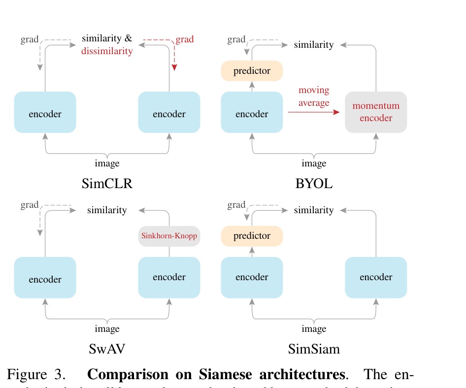
Figure 3: Comparison on Siamese architectures. The encoder includes all layers that can be shared between both branches. The dash lines indicate the gradient propagation flow. In BYOL, SwAV, and SimSiam, the lack of a dash line implies stop-gradient, and their symmetrization is not illustrated for simplicity. The components in red are those missing in SimSiam.

图 3：孪生架构比较。编码器包含两支路可共享的所有层。虚线表示梯度传播路径。在 BYOL、SwAV 与 SimSiam 中，缺少虚线意味着 stop-gradient；为简洁未画出对称化。红色组件是 SimSiam 所缺。

Relation to BYOL

[15]. Our method can be thought of as “BYOL without the momentum encoder”, subject to many implementation differences. The momentum encoder may be beneficial for accuracy (Table 4), but it is not necessary for preventing collapsing. Given our hypothesis in Sec. 5, the $\eta$ sub-problem (8) can be solved by other optimizers, \eg, a gradient-based one. This may lead to a temporally smoother update on $\eta$. Although not directly related, the momentum encoder also produces a smoother version of $\eta$. We believe that other optimizers for solving (8) are also plausible, which can be a future research problem.

与 BYOL 的关系

[15]。我们的方法可视为「去掉动量编码器的 BYOL」，存在许多实现差异。动量编码器可能有利于准确率（表 4），但对防塌缩并非必要。根据第 5 节假设，$\eta$ 子问题 (8) 可用其他优化器求解，例如基于梯度的。这可能导致对 $\eta$ 更平滑的时间更新。虽非直接相关，动量编码器也产生更平滑版本的 $\eta$。我们相信求解 (8) 的其他优化器同样可行，可作为未来研究问题。

7 Conclusion

7 结论

We have explored Siamese networks with simple designs. The competitiveness of our minimalist method suggests that the Siamese shape of the recent methods can be a core reason for their effectiveness. Siamese networks are natural and effective tools for modeling invariance, which is a focus of representation learning. We hope our study will attract the community’s attention to the fundamental role of Siamese networks in representation learning.

我们探索了设计简单的孪生网络。这一极简方法的竞争力表明，近期方法的孪生形态可能是其有效性的核心原因。孪生网络是建模不变性的自然且有效工具，而不变性是表示学习的焦点。希望本研究引起社区对孪生网络在表示学习中根本角色的关注。

References

参考文献

[1] Yuki Markus Asano, Christian Rupprecht, and Andrea Vedaldi. Self-labelling via simultaneous clustering and representation learning. arXiv:1911.05371 , 2019.

[2] Philip Bachman, R Devon Hjelm, and William Buchwalter. Learning representations by maximizing mutual information across views. arXiv:1906.00910 , 2019.

[3] Luca Bertinetto, Jack Valmadre, Joao F Henriques, Andrea Vedaldi, and Philip HS Torr. Fully-convolutional Siamese networks for object tracking. In ECCV , 2016.

[4] Jane Bromley, Isabelle Guyon, Yann LeCun, Eduard Säckinger, and Roopak Shah. Signature verification using a “Siamese” time delay neural network. In NeurIPS , 1994.

[5] Mathilde Caron, Piotr Bojanowski, Armand Joulin, and Matthijs Douze. Deep clustering for unsupervised learning of visual features. In ECCV , 2018.

[6] Mathilde Caron, Piotr Bojanowski, Julien Mairal, and Armand Joulin. Unsupervised pre-training of image features on non-curated data. In ICCV , 2019.

[7] Mathilde Caron, Ishan Misra, Julien Mairal, Priya Goyal, Piotr Bojanowski, and Armand Joulin. Unsupervised learning of visual features by contrasting cluster assignments. arXiv:2006.09882 , 2020.

[8] Ting Chen, Simon Kornblith, Mohammad Norouzi, and Geoffrey Hinton. A simple framework for contrastive learning of visual representations. arXiv:2002.05709 , 2020.

[9] Xinlei Chen, Haoqi Fan, Ross Girshick, and Kaiming He. Improved baselines with momentum contrastive learning. arXiv:2003.04297 , 2020.

[10] Marco Cuturi. Sinkhorn distances: Lightspeed computation of optimal transport. In NeurIPS , 2013.

[11] Jia Deng, Wei Dong, Richard Socher, Li-Jia Li, Kai Li, and Li Fei-Fei. ImageNet: A large-scale hierarchical image database. In CVPR , 2009.

[12] Mark Everingham, Luc Van Gool, Christopher KI Williams, John Winn, and Andrew Zisserman. The PASCAL Visual Object Classes (VOC) Challenge. IJCV , 2010.

[13] Ross Girshick, Ilija Radosavovic, Georgia Gkioxari, Piotr Dollár, and Kaiming He. Detectron, 2018.

[14] Priya Goyal, Piotr Dollár, Ross Girshick, Pieter Noordhuis, Lukasz Wesolowski, Aapo Kyrola, Andrew Tulloch, Yangqing Jia, and Kaiming He. Accurate, large minibatch SGD: Training ImageNet in 1 hour. arXiv:1706.02677 , 2017.

[15] Jean-Bastien Grill, Florian Strub, Florent Altché, Corentin Tallec, Pierre H. Richemond, Elena Buchatskaya, Carl Doersch, Bernardo Avila Pires, Zhaohan Daniel Guo, Mohammad Gheshlaghi Azar, Bilal Piot, Koray Kavukcuoglu, Rémi Munos, and Michal Valko. Bootstrap your own latent: A new approach to self-supervised learning. arXiv:2006.07733v1 , 2020.

[16] Raia Hadsell, Sumit Chopra, and Yann LeCun. Dimensionality reduction by learning an invariant mapping. In CVPR , 2006.

[17] Kaiming He, Haoqi Fan, Yuxin Wu, Saining Xie, and Ross Girshick. Momentum contrast for unsupervised visual representation learning. arXiv:1911.05722 , 2019.

[18] Kaiming He, Georgia Gkioxari, Piotr Dollár, and Ross Girshick. Mask R-CNN. In ICCV , 2017.

[19] Kaiming He, Xiangyu Zhang, Shaoqing Ren, and Jian Sun. Deep residual learning for image recognition. In CVPR , 2016.

[20] R Devon Hjelm, Alex Fedorov, Samuel Lavoie-Marchildon, Karan Grewal, Adam Trischler, and Yoshua Bengio. Learning deep representations by mutual information estimation and maximization. In ICLR , 2019.

[21] Olivier J. Hénaff, Aravind Srinivas, Jeffrey De Fauw, Ali Razavi, Carl Doersch, S. M. Ali Eslami, and Aaron van den Oord. Data-efficient image recognition with contrastive predictive coding. arXiv:1905.09272v2 , 2019.

[22] Sergey Ioffe and Christian Szegedy. Batch normalization: Accelerating deep network training by reducing internal covariate shift. In ICML , 2015.

[23] Gregory Koch, Richard Zemel, and Ruslan Salakhutdinov. Siamese neural networks for one-shot image recognition. In ICML deep learning workshop , 2015.

[24] Alex Krizhevsky. Learning multiple layers of features from tiny images. Tech Report , 2009.

[25] Yann LeCun, Bernhard Boser, John S Denker, Donnie Henderson, Richard E Howard, Wayne Hubbard, and Lawrence D Jackel. Backpropagation applied to handwritten zip code recognition. Neural computation , 1989.

[26] Tsung-Yi Lin, Michael Maire, Serge Belongie, James Hays, Pietro Perona, Deva Ramanan, Piotr Dollár, and C Lawrence Zitnick. Microsoft COCO: Common objects in context. In ECCV . 2014.

[27] Ilya Loshchilov and Frank Hutter. SGDR: Stochastic gradient descent with warm restarts. In ICLR , 2017.

[28] James MacQueen et al. Some methods for classification and analysis of multivariate observations. 1967.

[29] Ishan Misra and Laurens van der Maaten. Self-supervised learning of pretext-invariant representations. arXiv:1912.01991 , 2019.

[30] Aaron van den Oord, Yazhe Li, and Oriol Vinyals. Representation learning with contrastive predictive coding. arXiv:1807.03748 , 2018.

[31] Adam Paszke, Sam Gross, Francisco Massa, Adam Lerer, James Bradbury, Gregory Chanan, Trevor Killeen, Zeming Lin, Natalia Gimelshein, Luca Antiga, et al. PyTorch: An imperative style, high-performance deep learning library. In NeurIPS , 2019.

[32] Shaoqing Ren, Kaiming He, Ross Girshick, and Jian Sun. Faster R-CNN: Towards real-time object detection with region proposal networks. In NeurIPS , 2015.

[33] Tim Salimans and Diederik P Kingma. Weight normalization: A simple reparameterization to accelerate training of deep neural networks. In NeurIPS , 2016.

[34] Yaniv Taigman, Ming Yang, MarcAurelio Ranzato, and Lior Wolf. DeepFace: Closing the gap to human-level performance in face verification. In CVPR , 2014.

[35] Yonglong Tian, Dilip Krishnan, and Phillip Isola. Contrastive multiview coding. arXiv:1906.05849 , 2019.

[36] Zhirong Wu, Yuanjun Xiong, Stella Yu, and Dahua Lin. Unsupervised feature learning via non-parametric instance discrimination. In CVPR , 2018.

[37] Mang Ye, Xu Zhang, Pong C Yuen, and Shih-Fu Chang. Unsupervised embedding learning via invariant and spreading instance feature. In CVPR , 2019.

[38] Yang You, Igor Gitman, and Boris Ginsburg. Large batch training of convolutional networks. arXiv:1708.03888 , 2017.

Appendix A Implementation Details

附录 A 实现细节

Unsupervised pre-training.

Our implementation follows the practice of existing works [36, 17, 8, 9, 15].

无监督预训练。

实现沿用已有工作实践 [36, 17, 8, 9, 15]。

Data augmentation. We describe data augmentation using the PyTorch [31] notations. Geometric augmentation is RandomResizedCrop with scale in $[0.2,1.0]$ [36] and RandomHorizontalFlip. Color augmentation is ColorJitter with {brightness, contrast, saturation, hue} strength of {0.4, 0.4, 0.4, 0.1} with an applying probability of 0.8, and RandomGrayscale with an applying probability of 0.2. Blurring augmentation [8] has a Gaussian kernel with std in $[0.1,2.0]$.

数据增强。用 PyTorch [31] 记号描述数据增强。几何增强为 scale 在 $[0.2,1.0]$ 的 RandomResizedCrop [36] 与 RandomHorizontalFlip。颜色增强为 {brightness, contrast, saturation, hue} 强度 {0.4, 0.4, 0.4, 0.1}、施加概率 0.8 的 ColorJitter，以及施加概率 0.2 的 RandomGrayscale。模糊增强 [8] 使用 std 在 $[0.1,2.0]$ 的高斯核。

Initialization. The convolution and fc layers follow the default PyTorch initializers. Note that by default PyTorch initializes fc layers’ weight and bias by a uniform distribution $\mathcal{U}(-\sqrt{k},\sqrt{k})$ where $k{=}\frac{1}{\text{in\_channels}}$. Models with substantially different fc initializers (\eg, a fixed std of 0.01) may not converge. Moreover, similar to the implementation of [8], we initialize the scale parameters as 0 [14] in the last BN layer for every residual block.

初始化。卷积与 fc 层遵循 PyTorch 默认初始化器。注意默认下 PyTorch 用均匀分布 $\mathcal{U}(-\sqrt{k},\sqrt{k})$（$k{=}\frac{1}{\text{in\_channels}}$）初始化 fc 层权重与偏置。fc 初始化器差异过大（例如固定 std 0.01）的模型可能不收敛。此外，类似 [8] 的实现，我们把每个残差块最后 BN 层的尺度参数初始化为 0 [14]。

Weight decay. We use a weight decay of 0.0001 for all parameter layers, including the BN scales and biases, in the SGD optimizer. This is in contrast to the implementation of [8, 15] that excludes BN scales and biases from weight decay in their LARS optimizer.

权重衰减。SGD 优化器中对所有参数层（包括 BN 尺度与偏置）使用权重衰减 0.0001。这与 [8, 15] 在其 LARS 优化器中把 BN 尺度与偏置排除出权重衰减的实现相反。

Linear evaluation.

Given the pre-trained network, we train a supervised linear classifier on frozen features, which are from ResNet’s global average pooling layer (pool5). The linear classifier training uses base $lr\!=\!0.02$ with a cosine decay schedule for 90 epochs, weight decay$\penalty\ \!=\!0$, momentum$\penalty\ \!=\!0.9$, batch size$\penalty\ \!=\!4096$ with a LARS optimizer [38]. We have also tried the SGD optimizer following [17] with base $lr\!=\!30.0$, weight decay$\penalty\ \!=\!0$, momentum$\penalty\ \!=\!0.9$, and batch size$\penalty\ \!=\!256$, which gives $\scriptstyle\sim$1% lower accuracy. After training the linear classifier, we evaluate it on the center $224{\times}224$ crop in the validation set.

线性评估。

给定预训练网络，我们在冻结特征上训练有监督线性分类器，特征来自 ResNet 的全局平均池化层（pool5）。线性分类器训练使用基础 $lr\!=\!0.02$、余弦衰减 90 epoch、权重衰减$\penalty\ \!=\!0$、动量$\penalty\ \!=\!0.9$、batch$\penalty\ \!=\!4096$ 与 LARS 优化器 [38]。我们也试过沿用 [17] 的 SGD：基础 $lr\!=\!30.0$、权重衰减$\penalty\ \!=\!0$、动量$\penalty\ \!=\!0.9$、batch$\penalty\ \!=\!256$，准确率约低 $\scriptstyle\sim$1%。训练线性分类器后，在验证集中心 $224{\times}224$ 裁剪上评估。

Appendix B Additional Ablations on ImageNet

附录 B ImageNet 上的额外消融

The following table reports the SimSiam results \vsthe output dimension $d$:

下表报告 SimSiam 结果相对输出维度 $d$：

It benefits from a larger $d$ and gets saturated at $d\!=\!\text{2048}$. This is unlike existing methods [36, 17, 8, 15] whose accuracy is saturated when $d$ is 256 or 512.

它受益于更大的 $d$，并在 $d\!=\!\text{2048}$ 饱和。这与已有方法 [36, 17, 8, 15] 在 $d$ 为 256 或 512 时即饱和不同。

In this table, the prediction MLP’s hidden layer dimension is always 1/4 of the output dimension. We find that this bottleneck structure is more robust. If we set the hidden dimension to be equal to the output dimension, the training can be less stable or fail in some variants of our exploration. We hypothesize that this bottleneck structure, which behaves like an auto-encoder, can force the predictor to digest the information. We recommend to use this bottleneck structure for our method.

该表中预测 MLP 隐层维度恒为输出维度的 1/4。我们发现该瓶颈结构更稳健。若把隐层维度设为等于输出维度，训练在我们探索的某些变体中可能不够稳定或失败。我们假设该瓶颈结构类似自编码器，可迫使预测器消化信息。建议对我们的方法使用该瓶颈结构。

Appendix C Reproducing Related Methods

附录 C 复现相关方法

Our comparison in Table 4 is based on our reproduction of the related methods. We re-implement the related methods as faithfully as possible following each individual paper. In addition, we are able to improve SimCLR, MoCo v2, and SwAV by small and straightforward modifications: specifically, we use 3 layers in the projection MLP in SimCLR and SwAV (\vsoriginally 2), and use symmetrized loss for MoCo v2 (\vsoriginally asymmetric). Table C.1 compares our reproduction of these methods with the original papers’ results (if available). Our reproduction has better results for SimCLR, MoCo v2, and SwAV (denoted as “+” in Table 4), and has at least comparable results for BYOL.

表 4 的比较基于我们对相关方法的复现。我们尽可能忠实按各论文重实现。此外，通过小而直接的修改改进了 SimCLR、MoCo v2 与 SwAV：具体地，SimCLR 与 SwAV 的投影 MLP 用 3 层（相对原先 2 层），MoCo v2 用对称损失（相对原先非对称）。表 C.1 把我们的复现与原论文结果（若有）比较。对 SimCLR、MoCo v2 与 SwAV，复现结果更好（表 4 中记为「+」）；对 BYOL 至少可比。

	SimCLR	MoCo v2	BYOL	SwAV
epoch	200	800	1000	200	800	300	800	1000	400
origin	66.6	68.3	69.3	67.5	71.1	72.5	-	74.3	70.1
repro.	68.3	70.4	-	69.9	72.2	72.4	74.3	-	70.7

Table C.1: Our reproduction \vsoriginal papers’ results. All are based on ResNet-50 pre-trained with two 224$\times$224 crops.

	SimCLR	MoCo v2	BYOL	SwAV
epoch	200	800	1000	200	800	300	800	1000	400
origin	66.6	68.3	69.3	67.5	71.1	72.5	-	74.3	70.1
repro.	68.3	70.4	-	69.9	72.2	72.4	74.3	-	70.7

表 C.1：我们的复现 \vs 原论文结果。均基于以两份 224$\times$224 裁剪预训练的 ResNet-50。

Appendix D CIFAR Experiments

附录 D CIFAR 实验

We have observed similar behaviors of SimSiam in the CIFAR-10 dataset [24]. The implementation is similar to that in ImageNet. We use SGD with base $lr\!=\!0.03$ and a cosine decay schedule for 800 epochs, weight decay$\penalty\ \!=\!0.0005$, momentum$\penalty\ \!=\!0.9$, and batch size$\penalty\ \!=\!512$. The input image size is 32$\times$32. We do not use blur augmentation. The backbone is the CIFAR variant of ResNet-18 [19], followed by a 2-layer projection MLP. The outputs are 2048-d.

我们在 CIFAR-10 数据集 [24] 上观察到 SimSiam 的类似行为。实现与 ImageNet 类似。使用基础 $lr\!=\!0.03$、余弦衰减 800 epoch 的 SGD，权重衰减$\penalty\ \!=\!0.0005$，动量$\penalty\ \!=\!0.9$，batch$\penalty\ \!=\!512$。输入图像大小 32$\times$32。不使用模糊增强。骨干为 CIFAR 变体的 ResNet-18 [19]，后接 2 层投影 MLP。输出为 2048 维。

Figure D.1 shows the kNN classification accuracy (left) and the linear evaluation (right). Similar to the ImageNet observations, SimSiam achieves a reasonable result and does not collapse. We compare with SimCLR [8] trained with the same setting. Interestingly, the training curves are similar between SimSiam and SimCLR. SimSiam is slightly better by 0.7% under this setting.

图 D.1 给出 kNN 分类准确率（左）与线性评估（右）。与 ImageNet 观察类似，SimSiam 取得合理结果且不塌缩。与同一设定下训练的 SimCLR [8] 比较。有趣的是，SimSiam 与 SimCLR 的训练曲线相似。该设定下 SimSiam 略优 0.7%。

	acc. (%)
SimCLR	91.1
SimSiam	91.8

Figure D.1: CIFAR-10 experiments. Left: validation accuracy of kNN classification as a monitor during pre-training. Right: linear evaluation accuracy. The backbone is ResNet-18.

	acc. (%)
SimCLR	91.1
SimSiam	91.8

图 D.1：CIFAR-10 实验。左：预训练期间作为监视的 kNN 分类验证准确率。右：线性评估准确率。骨干为 ResNet-18。