SimCSE: Simple Contrastive Learning of Sentence Embeddings
Proceedings of the 2021 Conference on Empirical Methods in Natural Language Processing, pages 6894–6910
November 7–11, 2021. ©2021 Association for Computational Linguistics
SimCSE: Simple Contrastive Learning of Sentence Embeddings
∗The first two authors contributed equally (listed in alphabetical order). This work was done when Xingcheng visited the Princeton NLP group remotely.
Abstract
摘要
This paper presents SimCSE, a simple contrastive learning framework that greatly advances the state-of-the-art sentence embeddings. We first describe an unsupervised approach, which takes an input sentence and predicts itself in a contrastive objective, with only standard dropout used as noise. This simple method works surprisingly well, performing on par with previous supervised counterparts. We find that dropout acts as minimal data augmentation and removing it leads to a representation collapse. Then, we propose a supervised approach, which incorporates annotated pairs from natural language inference datasets into our contrastive learning framework, by using “entailment” pairs as positives and “contradiction” pairs as hard negatives. We evaluate SimCSE on standard semantic textual similarity (STS) tasks, and our unsupervised and supervised models using BERT achieve an average of 76.3% and 81.6% Spearman’s correlation respectively, a 4.2% and 2.2% improvement compared to previous best results. We also show—both theoretically and empirically—that contrastive learning objective regularizes pre-trained embeddings’ anisotropic space to be more uniform, and it better aligns positive pairs when supervised signals are available.[^1]
本文提出 SimCSE,这是一个简单的对比学习框架,显著推进了句子嵌入的最好水平。我们首先给出一种无监督方法:把输入句子本身放到对比目标里去预测,噪声只用标准的 dropout。这一简单做法出人意料地有效,表现已经能与此前的有监督方法持平。我们发现,dropout 起到了最轻微的数据增广作用;去掉它,表示就会崩塌。随后,我们提出一种有监督方法,把自然语言推断数据集中的标注句子对纳入同一套对比学习框架:把“蕴涵”对当作正样本,把“矛盾”对当作困难负样本。我们在标准的语义文本相似度(STS)任务上评估 SimCSE,使用 BERT 时,无监督和有监督模型的平均 Spearman 相关系数分别达到 76.3% 和 81.6%,比此前最好结果分别高出 4.2 和 2.2 个百分点。我们还从理论和实验两方面表明:对比学习目标会把预训练嵌入的各向异性空间约束得更均匀;在有监督信号时,它还能更好地对齐正样本对。[^1]
[^1]: Our code and pre-trained models are publicly available at https://github.com/princeton-nlp/SimCSE.
[^1]: 代码和预训练模型公开发布于 https://github.com/princeton-nlp/SimCSE。
1 Introduction
1 引言
Learning universal sentence embeddings is a fundamental problem in natural language processing and has been studied extensively in the literature (Kiros et al., 2015; Hill et al., 2016; Conneau et al., 2017; Logeswaran and Lee, 2018; Cer et al., 2018; Reimers and Gurevych, 2019, inter alia). In this work, we advance state-of-the-art sentence embedding methods and demonstrate that a contrastive objective can be extremely effective when coupled with pre-trained language models such as BERT (Devlin et al., 2019) or RoBERTa (Liu et al., 2019). We present SimCSE, a simple contrastive sentence embedding framework, which can produce superior sentence embeddings, from either unlabeled or labeled data.
学习通用句子嵌入是自然语言处理中的一个基本问题,文献中已有大量研究(Kiros et al., 2015; Hill et al., 2016; Conneau et al., 2017; Logeswaran and Lee, 2018; Cer et al., 2018; Reimers and Gurevych, 2019, inter alia)。本文推进句子嵌入方法的最好水平,并表明:当对比目标与 BERT(Devlin et al., 2019)或 RoBERTa(Liu et al., 2019)这类预训练语言模型结合时,可以非常有效。我们提出 SimCSE 这一简单的对比句子嵌入框架,无论是从无标注数据还是从有标注数据,都能得到更好的句子嵌入。
Our unsupervised SimCSE simply predicts the input sentence itself with only dropout (Srivastava et al., 2014) used as noise (Figure 1(a)). In other words, we pass the same sentence to the pre-trained encoder twice: by applying the standard dropout twice, we can obtain two different embeddings as “positive pairs”. Then we take other sentences in the same mini-batch as “negatives”, and the model predicts the positive one among negatives. Although it may appear strikingly simple, this approach outperforms training objectives such as predicting next sentences (Logeswaran and Lee, 2018) and discrete data augmentation (e.g., word deletion and replacement) by a large margin, and even matches previous supervised methods. Through careful analysis, we find that dropout acts as minimal “data augmentation” of hidden representations, while removing it leads to a representation collapse.
我们的无监督 SimCSE 只是预测输入句子本身,噪声只用 dropout(Srivastava et al., 2014)(图 1(a))。换句话说,我们把同一句话两次送入预训练编码器:通过两次施加标准 dropout,可以得到两个不同的嵌入,作为“正样本对”。然后把同一小批量中的其他句子当作“负样本”,模型要在这些负样本中找出那个正样本。尽管看起来极其简单,这一做法大幅优于预测下一句(Logeswaran and Lee, 2018)以及离散数据增广(例如删词和替换)这类训练目标,甚至能与此前的有监督方法持平。经过仔细分析,我们发现 dropout 相当于对隐表示做最轻微的“数据增广”;去掉它,表示就会崩塌。
Our supervised SimCSE builds upon the recent success of using natural language inference (NLI) datasets for sentence embeddings (Conneau et al., 2017; Reimers and Gurevych, 2019) and incorporates annotated sentence pairs in contrastive learning (Figure 1(b)). Unlike previous work that casts it as a 3-way classification task (entailment, neutral and contradiction), we leverage the fact that entailment pairs can be naturally used as positive instances. We also find that adding corresponding contradiction pairs as hard negatives further improves performance. This simple use of NLI datasets achieves a substantial improvement compared to prior methods using the same datasets. We also compare to other labeled sentence-pair datasets and find that NLI datasets are especially effective for learning sentence embeddings.
我们的有监督 SimCSE 建立在近来用自然语言推断(NLI)数据集学习句子嵌入的成功之上(Conneau et al., 2017; Reimers and Gurevych, 2019),并把带标注的句子对纳入对比学习(图 1(b))。与以往把它做成三分类任务(蕴涵、中立和矛盾)不同,我们利用的是:蕴涵对本来就可以当作正样本。我们还发现,把对应的矛盾对作为困难负样本,可以进一步提高表现。这样简单地使用 NLI 数据,比此前使用同一批数据的方法有明显提升。我们还与其他带标注的句子对数据集做了比较,发现 NLI 数据对学习句子嵌入尤为有效。
To better understand the strong performance of SimCSE, we borrow the analysis tool from Wang and Isola (2020), which takes alignment between semantically-related positive pairs and uniformity of the whole representation space to measure the quality of learned embeddings. Through empirical analysis, we find that our unsupervised SimCSE essentially improves uniformity while avoiding degenerated alignment via dropout noise, thus improving the expressiveness of the representations. The same analysis shows that the NLI training signal can further improve alignment between positive pairs and produce better sentence embeddings. We also draw a connection to the recent findings that pre-trained word embeddings suffer from anisotropy (Ethayarajh, 2019; Li et al., 2020) and prove that—through a spectrum perspective—the contrastive learning objective “flattens” the singular value distribution of the sentence embedding space, hence improving uniformity.
为了更好地理解 SimCSE 的出色表现,我们借用 Wang and Isola(2020)的分析工具:用语义相关正样本对之间的对齐(alignment),以及整个表示空间的均匀性(uniformity),来衡量学到的嵌入质量。通过实证分析,我们发现无监督 SimCSE 本质上是在改善均匀性,同时又借助 dropout 噪声避免对齐退化,从而提升表示的表达能力。同一套分析还表明,NLI 训练信号能进一步改善正样本对的对齐,得到更好的句子嵌入。我们还把这一点与近来的发现联系起来:预训练词嵌入存在各向异性(Ethayarajh, 2019; Li et al., 2020);并从频谱角度证明,对比学习目标会把句子嵌入空间的奇异值分布“压平”,从而改善均匀性。
We conduct a comprehensive evaluation of SimCSE on seven standard semantic textual similarity (STS) tasks (Agirre et al., 2012, 2013, 2014, 2015, 2016; Cer et al., 2017; Marelli et al., 2014) and seven transfer tasks (Conneau and Kiela, 2018). On the STS tasks, our unsupervised and supervised models achieve a 76.3% and 81.6% averaged Spearman’s correlation respectively using BERT, a 4.2% and 2.2% improvement compared to previous best results. We also achieve competitive performance on the transfer tasks. Finally, we identify an incoherent evaluation issue in the literature and consolidate results of different settings for future work in evaluation of sentence embeddings.
我们在七项标准语义文本相似度(STS)任务(Agirre et al., 2012, 2013, 2014, 2015, 2016; Cer et al., 2017; Marelli et al., 2014)以及七项迁移任务(Conneau and Kiela, 2018)上对 SimCSE 做了全面评估。在 STS 任务上,使用 BERT 时,无监督和有监督模型的平均 Spearman 相关系数分别达到 76.3% 和 81.6%,比此前最好结果分别高出 4.2 和 2.2 个百分点。在迁移任务上,我们也取得了有竞争力的表现。最后,我们指出文献中评估设定并不一致的问题,并把不同设定下的结果整理出来,供后续句子嵌入评估工作使用。
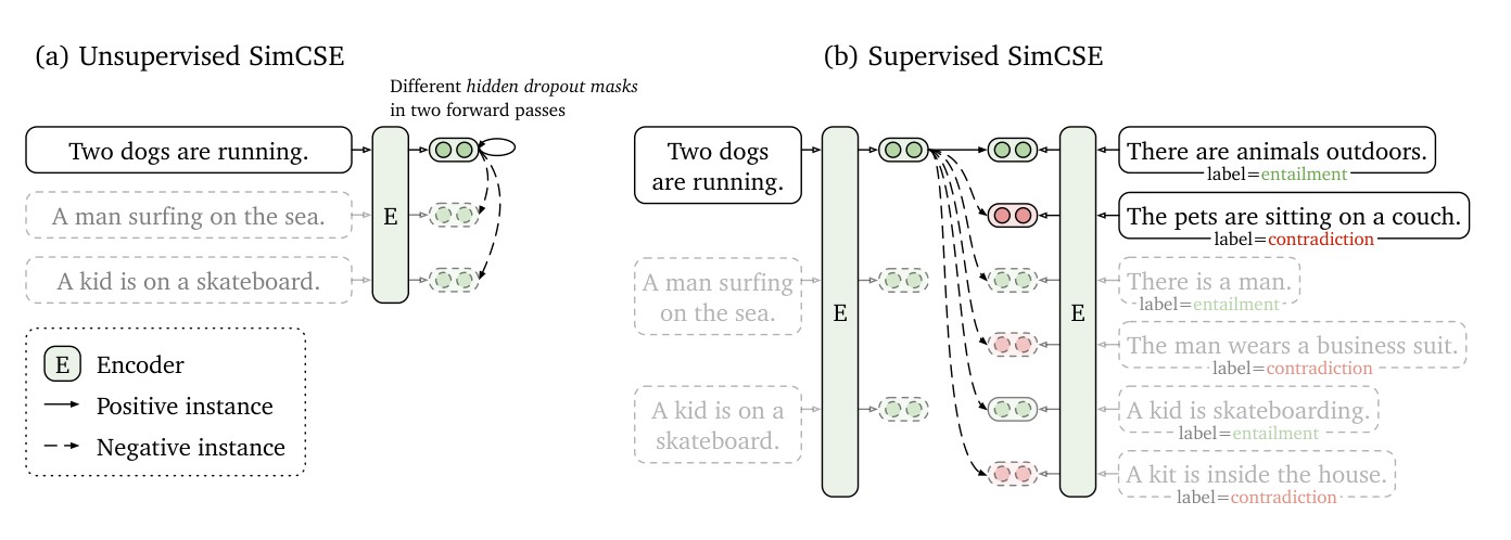
Figure 1: (a) Unsupervised SimCSE predicts the input sentence itself from in-batch negatives, with different hidden dropout masks applied. (b) Supervised SimCSE leverages the NLI datasets and takes the entailment (premise-hypothesis) pairs as positives, and contradiction pairs as well as other in-batch instances as negatives.
图 1:(a) 无监督 SimCSE 从批内负样本中预测输入句子本身,两次前向传播使用不同的隐层 dropout 掩码。(b) 有监督 SimCSE 利用 NLI 数据集,把蕴涵(前提–假设)对当作正样本,并把矛盾对以及其他批内实例当作负样本。
2 Background: Contrastive Learning
2 背景:对比学习
Contrastive learning aims to learn effective representation by pulling semantically close neighbors together and pushing apart non-neighbors (Hadsell et al., 2006). It assumes a set of paired examples , where and are semantically related. We follow the contrastive framework in Chen et al. (2020) and take a cross-entropy objective with in-batch negatives (Chen et al., 2017; Henderson et al., 2017): let and denote the representations of and , the training objective for with a mini-batch of pairs is:
对比学习的目标是学到有效的表示:把语义相近的邻居拉近,把非邻居推开(Hadsell et al., 2006)。它假设有一组成对样本 ,其中 与 在语义上相关。我们沿用 Chen et al.(2020)的对比框架,并采用带批内负样本的交叉熵目标(Chen et al., 2017; Henderson et al., 2017):用 和 表示 与 的表示,则对一个大小为 的小批量中的 ,训练目标为:
where is a temperature hyperparameter and is the cosine similarity . In this work, we encode input sentences using a pre-trained language model such as BERT (Devlin et al., 2019) or RoBERTa (Liu et al., 2019): , and then fine-tune all the parameters using the contrastive learning objective (Eq. 1).
其中 是温度超参数, 是余弦相似度 。本文用 BERT(Devlin et al., 2019)或 RoBERTa(Liu et al., 2019)这类预训练语言模型对输入句子编码:,再用对比学习目标(公式 1)微调全部参数。
Positive instances.
正样本。
One critical question in contrastive learning is how to construct pairs. In visual representations, an effective solution is to take two random transformations of the same image (e.g., cropping, flipping, distortion and rotation) as and (Dosovitskiy et al., 2014). A similar approach has been recently adopted in language representations (Wu et al., 2020; Meng et al., 2021) by applying augmentation techniques such as word deletion, reordering, and substitution. However, data augmentation in NLP is inherently difficult because of its discrete nature. As we will see in §3, simply using standard dropout on intermediate representations outperforms these discrete operators.
对比学习中的一个关键问题,是如何构造 对。在视觉表示里,一个有效做法是把同一张图像的两次随机变换(例如裁剪、翻转、扭曲和旋转)分别作为 和 (Dosovitskiy et al., 2014)。语言表示近来也采用了类似思路(Wu et al., 2020; Meng et al., 2021),使用删词、重排和替换等增广。然而,由于文本是离散的,NLP 中的数据增广本质上就很难。我们将在第 3 节看到,仅仅在中间表示上使用标准 dropout,就已经优于这些离散操作。
In NLP, a similar contrastive learning objective has been explored in different contexts (Henderson et al., 2017; Gillick et al., 2019; Karpukhin et al., 2020). In these cases, are collected from supervised datasets such as question-passage pairs. Because of the distinct nature of and , these approaches always use a dual-encoder framework, i.e., using two independent encoders and for and . For sentence embeddings, Logeswaran and Lee (2018) also use contrastive learning with a dual-encoder approach, by forming current sentence and next sentence as .
在 NLP 中,类似的对比学习目标已在不同情境下被探索过(Henderson et al., 2017; Gillick et al., 2019; Karpukhin et al., 2020)。这些情形里, 来自问句–段落对这类有监督数据。由于 与 性质不同,这些方法总是使用双编码器框架,也就是用两个独立的编码器 和 分别处理 和 。在句子嵌入方面,Logeswaran and Lee(2018)也用对比学习加双编码器,把当前句和下一句组成 。
Alignment and uniformity.
对齐与均匀性。
Recently, Wang and Isola (2020) identify two key properties related to contrastive learning—alignment and uniformity—and propose to use them to measure the quality of representations. Given a distribution of positive pairs , alignment calculates expected distance between embeddings of the paired instances (assuming representations are already normalized):
近来,Wang and Isola(2020)指出与对比学习相关的两个关键性质——对齐(alignment)和均匀性(uniformity)——并提议用它们来衡量表示质量。给定正样本对的分布 ,对齐计算成对实例嵌入之间的期望距离(假定表示已经归一化):
On the other hand, uniformity measures how well the embeddings are uniformly distributed:
另一方面,均匀性衡量嵌入在空间中分布得有多均匀:
where denotes the data distribution. These two metrics are well aligned with the objective of contrastive learning: positive instances should stay close and embeddings for random instances should scatter on the hypersphere. In the following sections, we will also use the two metrics to justify the inner workings of our approaches.
其中 表示数据分布。这两个指标与对比学习的目标十分吻合:正样本应当靠近,随机实例的嵌入则应散布在超球面上。在后面各节中,我们也会用这两个指标来说明我们方法的内在机制。
3 Unsupervised SimCSE
3 无监督 SimCSE
The idea of unsupervised SimCSE is extremely simple: we take a collection of sentences and use . The key ingredient to get this to work with identical positive pairs is through the use of independently sampled dropout masks for and . In standard training of Transformers (Vaswani et al., 2017), there are dropout masks placed on fully-connected layers as well as attention probabilities (default ). We denote where is a random mask for dropout. We simply feed the same input to the encoder twice and get two embeddings with different dropout masks , and the training objective of SimCSE becomes:
无监督 SimCSE 的想法极其简单:取一组句子 ,并令 。要让完全相同的正样本对也能学起来,关键在于对 和 独立采样 dropout 掩码。在 Transformer 的标准训练中(Vaswani et al., 2017),全连接层以及注意力概率上都会放置 dropout 掩码(默认 )。我们记 ,其中 是随机的 dropout 掩码。我们只需把同一输入两次送入编码器,得到带有不同 dropout 掩码 的两个嵌入,于是 SimCSE 的训练目标变为:
for a mini-batch of sentences. Note that is just the standard dropout mask in Transformers and we do not add any additional dropout.
这里的小批量大小为 。需要注意的是, 就是 Transformer 里的标准 dropout 掩码,我们没有再额外添加 dropout。
Dropout noise as data augmentation.
把 dropout 噪声当作数据增广。
We view it as a minimal form of data augmentation: the positive pair takes exactly the same sentence, and their embeddings only differ in dropout masks. We compare this approach to other training objectives on the STS-B development set (Cer et al., 2017)[^2]. Table 1 compares our approach to common data augmentation techniques such as crop, word deletion and replacement, which can be viewed as and is a (random) discrete operator on . We note that even deleting one word would hurt performance and none of the discrete augmentations outperforms dropout noise.
我们把它看作最轻微的一种数据增广:正样本对用的是完全同一句话,它们的嵌入只在 dropout 掩码上不同。我们在 STS-B 开发集上把这一做法与其他训练目标做了比较(Cer et al., 2017)[^2]。表 1 把我们的方法与常见数据增广做了对比,例如裁剪、删词和替换,它们都可以写成 ,其中 是作用在 上的(随机)离散操作。我们注意到,即便只删一个词也会损害表现,而且没有任何一种离散增广超过 dropout 噪声。
[^2]: We randomly sample sentences from English Wikipedia and fine-tune BERT with learning rate = 3e-5, = 64. In all our experiments, no STS training sets are used.
[^2]: 我们从英文维基百科中随机采样 个句子,并用学习率 3e-5、 = 64 微调 BERT。在我们的全部实验中,都没有使用 STS 训练集。
Table 1: Comparison of data augmentations on STS-B development set (Spearman’s correlation). Crop %: keep % of the length; word deletion %: delete % words; Synonym replacement: use nlpaug (Ma, 2019) to randomly replace one word with its synonym; MLM %: use BERT to replace % of words.
| Data augmentation | STS-B | ||
|---|---|---|---|
| None (unsup. SimCSE) | 82.5 | ||
| Crop | 10% | 20% | 30% |
| 77.8 | 71.4 | 63.6 | |
| Word deletion | 10% | 20% | 30% |
| 75.9 | 72.2 | 68.2 | |
| Delete one word | 75.9 | ||
| w/o dropout | 74.2 | ||
| Synonym replacement | 77.4 | ||
| MLM 15% | 62.2 |
表 1:不同数据增广在 STS-B 开发集上的比较(Spearman 相关系数)。 Crop %:保留长度的 %;word deletion %:删除 % 的词;同义替换:用 nlpaug(Ma, 2019)随机把一个词换成同义词;MLM %:用 BERT 替换 % 的词。
| 数据增广 | STS-B | ||
|---|---|---|---|
| 无(无监督 SimCSE) | 82.5 | ||
| 裁剪 | 10% | 20% | 30% |
| 77.8 | 71.4 | 63.6 | |
| 删词 | 10% | 20% | 30% |
| 75.9 | 72.2 | 68.2 | |
| 删除一个词 | 75.9 | ||
| 去掉 dropout | 74.2 | ||
| 同义替换 | 77.4 | ||
| MLM 15% | 62.2 |
We also compare this self-prediction training objective to the next-sentence objective used in Logeswaran and Lee (2018), taking either one encoder or two independent encoders. As shown in Table 2, we find that SimCSE performs much better than the next-sentence objectives (82.5 vs 67.4 on STS-B) and using one encoder instead of two makes a significant difference in our approach.
我们还把这种“预测自身”的训练目标,与 Logeswaran and Lee(2018)使用的下一句目标做了比较,分别尝试一个编码器以及两个独立编码器。如表 2 所示,SimCSE 明显优于下一句目标(在 STS-B 上为 82.5 对 67.4);而且在我们的方法里,用一个编码器而不是两个,差别也很大。
Table 2: Comparison of different unsupervised objectives (STS-B development set, Spearman’s correlation). The two columns denote whether we use one encoder or two independent encoders. Next 3 sentences: randomly sample one from the next 3 sentences. Delete one word: delete one word randomly (see Table 1).
| Training objective | ||
|---|---|---|
| Next sentence | 67.1 | 68.9 |
| Next 3 sentences | 67.4 | 68.8 |
| Delete one word | 75.9 | 73.1 |
| Unsupervised SimCSE | 82.5 | 80.7 |
表 2:不同无监督目标的比较(STS-B 开发集,Spearman 相关系数)。 两列分别表示使用一个编码器,或使用两个独立编码器。Next 3 sentences:从随后 3 句中随机采样一句。Delete one word:随机删除一个词(见表 1)。
| 训练目标 | ||
|---|---|---|
| 下一句 | 67.1 | 68.9 |
| 随后 3 句中的一句 | 67.4 | 68.8 |
| 删除一个词 | 75.9 | 73.1 |
| 无监督 SimCSE | 82.5 | 80.7 |
Why does it work?
为什么有效?
To further understand the role of dropout noise in unsupervised SimCSE, we try out different dropout rates in Table 3 and observe that all the variants underperform the default dropout probability from Transformers. We find two extreme cases particularly interesting: “no dropout” () and “fixed 0.1” (using default dropout but the same dropout masks for the pair). In both cases, the resulting embeddings for the pair are exactly the same, and it leads to a dramatic performance degradation. We take the checkpoints of these models every 10 steps during training and visualize the alignment and uniformity metrics[^3] in Figure 2, along with a simple data augmentation model “delete one word”. As clearly shown, starting from pre-trained checkpoints, all models greatly improve uniformity. However, the alignment of the two special variants also degrades drastically, while our unsupervised SimCSE keeps a steady alignment, thanks to the use of dropout noise. It also demonstrates that starting from a pre-trained checkpoint is crucial, for it provides good initial alignment. At last, “delete one word” improves the alignment yet achieves a smaller gain on the uniformity metric, and eventually underperforms unsupervised SimCSE.
为了进一步理解 dropout 噪声在无监督 SimCSE 中的作用,我们在表 3 中尝试了不同的 dropout 率,发现所有变体都不如 Transformer 默认的 dropout 概率 。有两种极端情形尤其值得注意:“无 dropout”()和“固定 0.1”(仍用默认的 ,但对这一对样本使用同一张 dropout 掩码)。在这两种情形下,这对样本得到的嵌入完全相同,表现会大幅下降。我们在训练过程中每隔 10 步取出这些模型的检查点,并把对齐和均匀性指标[^3]画在图 2 中,同时加入一个简单的数据增广模型“删除一个词”。可以清楚看到,从预训练检查点出发,所有模型都大幅改善了均匀性。然而,那两个特殊变体的对齐也会急剧变差;而无监督 SimCSE 则靠 dropout 噪声保持了稳定的对齐。这也说明,从预训练检查点出发至关重要,因为它提供了良好的初始对齐。最后,“删除一个词”虽然改善了对齐,但在均匀性指标上的提升较小,最终仍不如无监督 SimCSE。
[^3]: We take STS-B pairs with a score higher than 4 as and all STS-B sentences as .
[^3]: 我们把评分高于 4 的 STS-B 句子对作为 ,并把 STS-B 中的全部句子作为 。
Table 3: Effects of different dropout probabilities on the STS-B development set (Spearman’s correlation, BERT). Fixed 0.1: default 0.1 dropout rate but apply the same dropout mask on both and .
| 0.0 | 0.01 | 0.05 | 0.1 | |
|---|---|---|---|---|
| STS-B | 71.1 | 72.6 | 81.1 | 82.5 |
| 0.15 | 0.2 | 0.5 | Fixed 0.1 | |
| STS-B | 81.4 | 80.5 | 71.0 | 43.6 |
表 3:不同 dropout 概率 在 STS-B 开发集上的影响(Spearman 相关系数,BERT)。 Fixed 0.1:默认 0.1 的 dropout 率,但对 和 使用同一张 dropout 掩码。
| 0.0 | 0.01 | 0.05 | 0.1 | |
|---|---|---|---|---|
| STS-B | 71.1 | 72.6 | 81.1 | 82.5 |
| 0.15 | 0.2 | 0.5 | Fixed 0.1 | |
| STS-B | 81.4 | 80.5 | 71.0 | 43.6 |
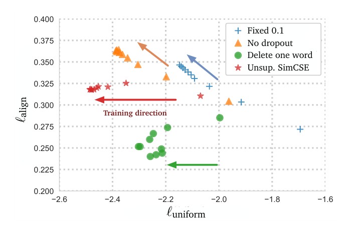
Figure 2: - plot for unsupervised SimCSE, “no dropout”, “fixed 0.1”, and “delete one word”. We visualize checkpoints every 10 training steps and the arrows indicate the training direction. For both and , lower numbers are better.
图 2:无监督 SimCSE、“无 dropout”、“固定 0.1”以及“删除一个词”的 - 图。我们每隔 10 个训练步可视化一次检查点,箭头表示训练方向。对 和 而言,数值越低越好。
4 Supervised SimCSE
4 有监督 SimCSE
We have demonstrated that adding dropout noise is able to keep a good alignment for positive pairs . In this section, we study whether we can leverage supervised datasets to provide better training signals for improving alignment of our approach. Prior work (Conneau et al., 2017; Reimers and Gurevych, 2019) has demonstrated that supervised natural language inference (NLI) datasets (Bowman et al., 2015; Williams et al., 2018) are effective for learning sentence embeddings, by predicting whether the relationship between two sentences is entailment, neutral or contradiction. In our contrastive learning framework, we instead directly take pairs from supervised datasets and use them to optimize Eq. 1.
我们已经表明,加入 dropout 噪声,能够为 这类正样本对保持良好的对齐。本节研究能否借助有监督数据集,为改善对齐提供更强的训练信号。已有工作(Conneau et al., 2017; Reimers and Gurevych, 2019)表明,有监督的自然语言推断(NLI)数据集(Bowman et al., 2015; Williams et al., 2018)对学习句子嵌入很有效,做法是预测两句之间的关系是蕴涵、中立还是矛盾。在我们的对比学习框架里,我们改为直接从有监督数据中取出 对,用来优化公式 1。
Choices of labeled data.
标注数据的选择。
We first explore which supervised datasets are especially suitable for constructing positive pairs . We experiment with a number of datasets with sentence-pair examples, including 1) QQP[^4]: Quora question pairs; 2) Flickr30k (Young et al., 2014): each image is annotated with 5 human-written captions and we consider any two captions of the same image as a positive pair; 3) ParaNMT (Wieting and Gimpel, 2018): a large-scale back-translation paraphrase dataset[^5]; and finally 4) NLI datasets: SNLI (Bowman et al., 2015) and MNLI (Williams et al., 2018).
我们首先考察哪些有监督数据集特别适合构造正样本对 。我们试验了若干带句子对样本的数据集,包括:1)QQP[^4]:Quora 问句对;2)Flickr30k(Young et al., 2014):每张图像配有 5 条人工撰写的描述,我们把同一图像的任意两条描述当作正样本对;3)ParaNMT(Wieting and Gimpel, 2018):一个大规模回译复述数据集[^5];以及最后 4)NLI 数据集:SNLI(Bowman et al., 2015)和 MNLI(Williams et al., 2018)。
[^5]: ParaNMT is automatically constructed by machine translation systems. Strictly speaking, we should not call it “supervised”. It underperforms our unsupervised SimCSE though.
[^5]: ParaNMT 是由机器翻译系统自动构造的。严格说来,不应称之为“有监督”。它的表现其实不如我们的无监督 SimCSE。
We train the contrastive learning model (Eq. 1) with different datasets and compare the results in Table 4. For a fair comparison, we also run experiments with the same # of training pairs. Among all the options, using entailment pairs from the NLI (SNLI + MNLI) datasets performs the best. We think this is reasonable, as the NLI datasets consist of high-quality and crowd-sourced pairs. Also, human annotators are expected to write the hypotheses manually based on the premises and two sentences tend to have less lexical overlap. For instance, we find that the lexical overlap (F1 measured between two bags of words) for the entailment pairs (SNLI + MNLI) is 39%, while they are 60% and 55% for QQP and ParaNMT.
我们用不同数据集训练对比学习模型(公式 1),并在表 4 中比较结果。为了公平比较,我们也在相同训练对数下做了实验。在所有选项中,使用来自 NLI(SNLI + MNLI)的蕴涵对效果最好。我们认为这是合理的,因为 NLI 数据集由高质量、众包得到的句子对组成。同时,标注者需要根据前提手工写出假设,两句的词汇重叠往往更少。例如,我们发现蕴涵对(SNLI + MNLI)的词汇重叠(以两个词袋之间的 F1 衡量)为 39%,而 QQP 和 ParaNMT 分别为 60% 和 55%。
Contradiction as hard negatives.
把矛盾对当作困难负样本。
Finally, we further take the advantage of the NLI datasets by using its contradiction pairs as hard negatives[^6]. In NLI datasets, given one premise, annotators are required to manually write one sentence that is absolutely true (entailment), one that might be true (neutral), and one that is definitely false (contradiction). Therefore, for each premise and its entailment hypothesis, there is an accompanying contradiction hypothesis[^7] (see Figure 1 for an example).
最后,我们进一步利用 NLI 数据集,把它的矛盾对当作困难负样本[^6]。在 NLI 数据中,给定一个前提,标注者需要手工写出一句绝对为真的句子(蕴涵)、一句可能为真的句子(中立),以及一句肯定为假的句子(矛盾)。因此,对每个前提及其蕴涵假设,都有一个配套的矛盾假设[^7](示例见图 1)。
[^6]: We also experimented with adding neutral hypotheses as hard negatives. See Section 6.3 for more discussion.
[^6]: 我们也试验过把中立假设当作困难负样本。更多讨论见第 6.3 节。
[^7]: In fact, one premise can have multiple contradiction hypotheses. In our implementation, we only sample one as the hard negative and we did not find a difference by using more.
Formally, we extend to , where is the premise, and are entailment and contradiction hypotheses. The training objective is then defined by ( is mini-batch size):
形式上,我们把 扩展为 ,其中 是前提, 和 分别是蕴涵假设和矛盾假设。训练目标 于是定义为( 为小批量大小):
As shown in Table 4, adding hard negatives can further improve performance (84.9 → 86.2) and this is our final supervised SimCSE. We also tried to add the ANLI dataset (Nie et al., 2020) or combine it with our unsupervised SimCSE approach, but didn’t find a meaningful improvement. We also considered a dual encoder framework in supervised SimCSE and it hurt performance (86.2 → 84.2).
如表 4 所示,加入困难负样本还能进一步提高表现(84.9 → 86.2),这就是我们最终的有监督 SimCSE。我们也尝试过加入 ANLI 数据集(Nie et al., 2020),或把它与无监督 SimCSE 结合,但都没有看到有意义的提升。我们还在有监督 SimCSE 中考虑过双编码器框架,结果损害了表现(86.2 → 84.2)。
Table 4: Comparisons of different supervised datasets as positive pairs. Results are Spearman’s correlations on the STS-B development set using BERT (we use the same hyperparameters as the final SimCSE model). Numbers in brackets denote the # of pairs. Sample: subsampling 134k positive pairs for a fair comparison among datasets; full: using the full dataset. In the last block, we use entailment pairs as positives and contradiction pairs as hard negatives (our final model).
| Dataset | sample | full |
|---|---|---|
| Unsup. SimCSE (1m) | - | 82.5 |
| QQP (134k) | 81.8 | 81.8 |
| Flickr30k (318k) | 81.5 | 81.4 |
| ParaNMT (5m) | 79.7 | 78.7 |
| SNLI+MNLI | ||
| entailment (314k) | 84.1 | 84.9 |
| neutral (314k)[^8] | 82.6 | 82.9 |
| contradiction (314k) | 77.5 | 77.6 |
| all (942k) | 81.7 | 81.9 |
| SNLI+MNLI | ||
| entailment + hard neg. | - | 86.2 |
| + ANLI (52k) | - | 85.0 |
表 4:把不同有监督数据集用作正样本对的比较。 结果为使用 BERT 在 STS-B 开发集上的 Spearman 相关系数(超参数与最终 SimCSE 模型相同)。括号中的数字表示对数。Sample:为了在数据集之间公平比较,子采样 134k 个正样本对;full:使用全部数据。在最后一组中,我们把蕴涵对当作正样本、把矛盾对当作困难负样本(即最终模型)。
| 数据集 | sample | full |
|---|---|---|
| 无监督 SimCSE(1m) | - | 82.5 |
| QQP(134k) | 81.8 | 81.8 |
| Flickr30k(318k) | 81.5 | 81.4 |
| ParaNMT(5m) | 79.7 | 78.7 |
| SNLI+MNLI | ||
| 蕴涵(314k) | 84.1 | 84.9 |
| 中立(314k)[^8] | 82.6 | 82.9 |
| 矛盾(314k) | 77.5 | 77.6 |
| 全部(942k) | 81.7 | 81.9 |
| SNLI+MNLI | ||
| 蕴涵 + 困难负样本 | - | 86.2 |
| + ANLI(52k) | - | 85.0 |
[^8]: Though our final model only takes entailment pairs as positive instances, here we also try taking neutral and contradiction pairs from the NLI datasets as positive pairs.
[^8]: 尽管最终模型只把蕴涵对当作正样本,这里我们也尝试把 NLI 数据中的中立对和矛盾对当作正样本。
5 Connection to Anisotropy
5 与各向异性的联系
Recent work identifies an anisotropy problem in language representations (Ethayarajh, 2019; Li et al., 2020), i.e., the learned embeddings occupy a narrow cone in the vector space, which severely limits their expressiveness. Gao et al. (2019) demonstrate that language models trained with tied input/output embeddings lead to anisotropic word embeddings, and this is further observed by Ethayarajh (2019) in pre-trained contextual representations. Wang et al. (2020) show that singular values of the word embedding matrix in a language model decay drastically: except for a few dominating singular values, all others are close to zero.
近期工作指出,语言表示存在各向异性问题(Ethayarajh, 2019; Li et al., 2020),也就是学到的嵌入只占据向量空间中一个狭窄的锥体,严重限制了表达能力。Gao et al.(2019)表明,输入/输出嵌入绑定训练的语言模型会导致各向异性的词嵌入;Ethayarajh(2019)进一步在预训练的上下文表示中观察到了这一点。Wang et al.(2020)表明,语言模型中词嵌入矩阵的奇异值衰减得非常快:除了少数几个占主导的奇异值,其余都接近于零。
A simple way to alleviate the problem is post-processing, either to eliminate the dominant principal components (Arora et al., 2017; Mu and Viswanath, 2018), or to map embeddings to an isotropic distribution (Li et al., 2020; Su et al., 2021). Another common solution is to add regularization during training (Gao et al., 2019; Wang et al., 2020). In this work, we show that—both theoretically and empirically—the contrastive objective can also alleviate the anisotropy problem.
缓解这一问题的一个简单办法是后处理:要么消去占主导的主成分(Arora et al., 2017; Mu and Viswanath, 2018),要么把嵌入映射到各向同性分布(Li et al., 2020; Su et al., 2021)。另一种常见做法是在训练时加入正则(Gao et al., 2019; Wang et al., 2020)。本文从理论和实验两方面表明,对比目标同样可以缓解各向异性问题。
The anisotropy problem is naturally connected to uniformity (Wang and Isola, 2020), both highlighting that embeddings should be evenly distributed in the space. Intuitively, optimizing the contrastive learning objective can improve uniformity (or ease the anisotropy problem), as the objective pushes negative instances apart. Here, we take a singular spectrum perspective—which is a common practice in analyzing word embeddings (Mu and Viswanath, 2018; Gao et al., 2019; Wang et al., 2020), and show that the contrastive objective can “flatten” the singular value distribution of sentence embeddings and make the representations more isotropic.
各向异性问题与均匀性(Wang and Isola, 2020)有着自然的联系,两者都强调嵌入应当在空间中均匀分布。直观上看,优化对比学习目标可以改善均匀性(或缓解各向异性),因为这一目标会把负样本推开。这里我们从奇异谱的角度出发——这是分析词嵌入时的常用做法(Mu and Viswanath, 2018; Gao et al., 2019; Wang et al., 2020)——并表明对比目标可以把句子嵌入的奇异值分布“压平”,使表示更加各向同性。
Following Wang and Isola (2020), the asymptotics of the contrastive learning objective (Eq. 1) can be expressed by the following equation when the number of negative instances approaches infinity (assuming is normalized):
沿用 Wang and Isola(2020),当负样本数目趋于无穷(并假定 已经归一化)时,对比学习目标(公式 1)的渐近形式可以写成:
$$\begin{aligned}
&-\frac{1}{\tau}\underset{(x,x^+)\sim p_{\mathrm{pos}}}{\mathbb{E}}\left[f(x)^{\top}f(x^+)\right]\
&+\underset{x\sim p_{\mathrm{data}}}{\mathbb{E}}\left[\log\underset{x^-\sim p_{\mathrm{data}}}{\mathbb{E}}\left[e^{f(x)^{\top}f(x^-)/\tau}\right]\right],
\end{aligned} \tag{6}$$
where the first term keeps positive instances similar and the second pushes negative pairs apart. When is uniform over finite samples , with , we can derive the following formula from the second term with Jensen’s inequality:
其中第一项让正样本保持相近,第二项把负样本对推开。当 在有限样本 上均匀,并令 时,可以由第二项结合 Jensen 不等式得到:
$$\begin{aligned}
&\underset{x\sim p_{\mathrm{data}}}{\mathbb{E}}\left[\log\underset{x^-\sim p_{\mathrm{data}}}{\mathbb{E}}\left[e^{f(x)^{\top}f(x^-)/\tau}\right]\right]\
=&\frac{1}{m}\sum_{i=1}^{m}\log\left(\frac{1}{m}\sum_{j=1}^{m}e^{\mathbf{h}i^{\top}\mathbf{h}j/\tau}\right)\
\geq&\frac{1}{\tau m^2}\sum{i=1}^{m}\sum{j=1}^{m}\mathbf{h}_i^{\top}\mathbf{h}_j.
\end{aligned} \tag{7}$$
Let be the sentence embedding matrix corresponding to , i.e., the -th row of is . Optimizing the second term in Eq. 6 essentially minimizes an upper bound of the summation of all elements in , i.e., .
令 为与 对应的句子嵌入矩阵,也就是 的第 行是 。优化公式 6 中的第二项,本质上是在最小化 所有元素之和的一个上界,即 。
Since we normalize , all elements on the diagonal of are 1 and then (the sum of all eigenvalues) is a constant. According to Merikoski (1984), if all elements in are positive, which is the case in most times according to Figure G.1, then is an upper bound for the largest eigenvalue of . When minimizing the second term in Eq. 6, we reduce the top eigenvalue of and inherently “flatten” the singular spectrum of the embedding space. Therefore, contrastive learning is expected to alleviate the representation degeneration problem and improve uniformity of sentence embeddings.
由于我们对 做了归一化, 对角线上的元素都是 1,于是 (全部特征值之和)是一个常数。根据 Merikoski(1984),如果 中的所有元素都为正——从图 G.1 看,多数时候确实如此——那么 就是 最大特征值的一个上界。最小化公式 6 中的第二项时,我们降低了 的最大特征值,从而在本质上把嵌入空间的奇异谱“压平”。因此,对比学习有望缓解表示退化问题,并改善句子嵌入的均匀性。
Compared to post-processing methods in Li et al. (2020); Su et al. (2021), which only aim to encourage isotropic representations, contrastive learning also optimizes for aligning positive pairs by the first term in Eq. 6, which is the key to the success of SimCSE. A quantitative analysis is given in §7.
与 Li et al.(2020);Su et al.(2021)中只鼓励各向同性表示的后处理方法相比,对比学习还会通过公式 6 中的第一项去对齐正样本对,而这正是 SimCSE 成功的关键。第 7 节给出了定量分析。
6 Experiment
6 实验
6.1 Evaluation Setup
6.1 评估设定
We conduct our experiments on 7 semantic textual similarity (STS) tasks. Note that all our STS experiments are fully unsupervised and no STS training sets are used. Even for supervised SimCSE, we simply mean that we take extra labeled datasets for training, following previous work (Conneau et al., 2017). We also evaluate 7 transfer learning tasks and provide detailed results in Appendix E. We share a similar sentiment with Reimers and Gurevych (2019) that the main goal of sentence embeddings is to cluster semantically similar sentences and hence take STS as the main result.
我们在 7 项语义文本相似度(STS)任务上开展实验。需要说明的是,我们所有的 STS 实验都是完全无监督的,没有使用任何 STS 训练集。即使是有监督 SimCSE,也只是指我们像以往工作(Conneau et al., 2017)那样,额外使用带标注的数据集来训练。我们还评估了 7 项迁移学习任务,详细结果见附录 E。我们与 Reimers and Gurevych(2019)持相近看法:句子嵌入的主要目标是把语义相近的句子聚在一起,因此把 STS 作为主要结果。
Semantic textual similarity tasks.
语义文本相似度任务。
We evaluate on 7 STS tasks: STS 2012–2016 (Agirre et al., 2012, 2013, 2014, 2015, 2016), STS Benchmark (Cer et al., 2017) and SICK-Relatedness (Marelli et al., 2014). When comparing to previous work, we identify invalid comparison patterns in published papers in the evaluation settings, including (a) whether to use an additional regressor, (b) Spearman’s vs Pearson’s correlation, and (c) how the results are aggregated (Table B.1). We discuss the detailed differences in Appendix B and choose to follow the setting of Reimers and Gurevych (2019) in our evaluation (no additional regressor, Spearman’s correlation, and “all” aggregation). We also report our replicated study of previous work as well as our results evaluated in a different setting in Table B.2 and Table B.3. We call for unifying the setting in evaluating sentence embeddings for future research.
我们在 7 项 STS 任务上评估:STS 2012–2016(Agirre et al., 2012, 2013, 2014, 2015, 2016)、STS Benchmark(Cer et al., 2017)以及 SICK-Relatedness(Marelli et al., 2014)。在与以往工作比较时,我们发现已发表论文的评估设定中存在一些不宜直接比较的情形,包括:(a) 是否使用额外的回归器;(b) 使用 Spearman 相关还是 Pearson 相关;(c) 结果如何汇总(表 B.1)。我们在附录 B 中讨论了这些差异的细节,并选择在评估中沿用 Reimers and Gurevych(2019)的设定(不加额外回归器、使用 Spearman 相关,以及 “all” 汇总方式)。我们也在表 B.2 和表 B.3 中报告了对以往工作的复现,以及在另一种设定下评估我们模型的结果。我们呼吁后续研究在句子嵌入评估中统一设定。
Training details.
训练细节。
We start from pre-trained checkpoints of BERT (Devlin et al., 2019) (uncased) or RoBERTa (Liu et al., 2019) (cased) and take the [CLS] representation as the sentence embedding[^9] (see §6.3 for comparison between different pooling methods). We train unsupervised SimCSE on randomly sampled sentences from English Wikipedia, and train supervised SimCSE on the combination of MNLI and SNLI datasets (314k). More training details can be found in Appendix A.
我们从 BERT(Devlin et al., 2019)(uncased)或 RoBERTa(Liu et al., 2019)(cased)的预训练检查点出发,并把 [CLS] 表示当作句子嵌入[^9](不同池化方法的比较见第 6.3 节)。无监督 SimCSE 在从英文维基百科随机采样的 个句子上训练;有监督 SimCSE 在 MNLI 与 SNLI 的合并数据(314k)上训练。更多训练细节见附录 A。
[^9]: There is an MLP layer over [CLS] in BERT’s original implementation and we keep it with random initialization.
[^9]: BERT 的原始实现里,[CLS] 之上有一个 MLP 层;我们保留这一层,并做随机初始化。
6.2 Main Results
6.2 主要结果
We compare unsupervised and supervised SimCSE to previous state-of-the-art sentence embedding methods on STS tasks. Unsupervised baselines include average GloVe embeddings (Pennington et al., 2014), average BERT or RoBERTa embeddings[^10], and post-processing methods such as BERT-flow (Li et al., 2020) and BERT-whitening (Su et al., 2021). We also compare to several recent methods using a contrastive objective, including 1) IS-BERT (Zhang et al., 2020), which maximizes the agreement between global and local features; 2) DeCLUTR (Giorgi et al., 2021), which takes different spans from the same document as positive pairs; 3) CT (Carlsson et al., 2021), which aligns embeddings of the same sentence from two different encoders.[^11] Other supervised methods include InferSent (Conneau et al., 2017), Universal Sentence Encoder (Cer et al., 2018), and SBERT/SRoBERTa (Reimers and Gurevych, 2019) with post-processing methods (BERT-flow, whitening, and CT). We provide more details of these baselines in Appendix C.
我们在 STS 任务上,把无监督和有监督 SimCSE 与此前最好的句子嵌入方法进行比较。无监督基线包括平均 GloVe 嵌入(Pennington et al., 2014)、平均 BERT 或 RoBERTa 嵌入[^10],以及 BERT-flow(Li et al., 2020)和 BERT-whitening(Su et al., 2021)这类后处理方法。我们还与若干使用对比目标的近期方法进行比较,包括:1)IS-BERT(Zhang et al., 2020),它最大化全局特征与局部特征之间的一致性;2)DeCLUTR(Giorgi et al., 2021),它把同一文档中的不同片段当作正样本对;3)CT(Carlsson et al., 2021),它对同一句子来自两个不同编码器的嵌入做对齐。[^11] 其他有监督方法包括 InferSent(Conneau et al., 2017)、Universal Sentence Encoder(Cer et al., 2018),以及带后处理(BERT-flow、whitening 和 CT)的 SBERT/SRoBERTa(Reimers and Gurevych, 2019)。这些基线的更多细节见附录 C。
[^10]: Following Su et al. (2021), we take the average of the first and the last layers, which is better than only taking the last.
[^10]: 沿用 Su et al.(2021),我们取第一层和最后一层的平均,这比只取最后一层更好。
[^11]: We do not compare to CLEAR (Wu et al., 2020), because they use their own version of pre-trained models, and the numbers appear to be much lower. Also note that CT is a concurrent work to ours.
[^11]: 我们没有与 CLEAR(Wu et al., 2020)比较,因为他们使用的是自己版本的预训练模型,而且数字看起来低很多。另外需要说明,CT 与本文是同期工作。
Table 5 shows the evaluation results on 7 STS tasks. SimCSE can substantially improve results on all the datasets with or without extra NLI supervision, greatly outperforming the previous state-of-the-art models. Specifically, our unsupervised SimCSE-BERT improves the previous best averaged Spearman’s correlation from 72.05% to 76.25%, even comparable to supervised baselines. When using NLI datasets, SimCSE-BERT further pushes the state-of-the-art results to 81.57%. The gains are more pronounced on RoBERTa encoders, and our supervised SimCSE achieves 83.76% with RoBERTa.
表 5 给出了 7 项 STS 任务上的评估结果。无论是否使用额外的 NLI 监督,SimCSE 都能在所有数据集上显著提升结果,大幅超过此前最好的模型。具体来说,我们的无监督 SimCSE-BERT 把此前最好的平均 Spearman 相关系数从 72.05% 提高到 76.25%,甚至已经可以与有监督基线相比。使用 NLI 数据后,SimCSE-BERT 进一步把最好结果推到 81.57%。在 RoBERTa 编码器上,提升更为明显:有监督 SimCSE 使用 RoBERTa 达到了 83.76%。
In Appendix E, we show that SimCSE also achieves on par or better transfer task performance compared to existing work, and an auxiliary MLM objective can further boost performance.
在附录 E 中我们表明,SimCSE 在迁移任务上的表现也与已有工作持平或更好,而且加入辅助的 MLM 目标还能进一步提高表现。
Table 5: Sentence embedding performance on STS tasks (Spearman’s correlation, “all” setting). We highlight the highest numbers among models with the same pre-trained encoder. ♣: results from Reimers and Gurevych (2019); ♥: results from Zhang et al. (2020); all other results are reproduced or reevaluated by ourselves. For BERT-flow (Li et al., 2020) and whitening (Su et al., 2021), we only report the “NLI” setting (see Table C.1).
| Model | STS12 | STS13 | STS14 | STS15 | STS16 | STS-B | SICK-R | Avg. |
|---|---|---|---|---|---|---|---|---|
| Unsupervised models | ||||||||
| GloVe embeddings (avg.)♣ | 55.14 | 70.66 | 59.73 | 68.25 | 63.66 | 58.02 | 53.76 | 61.32 |
| BERT (first-last avg.) | 39.70 | 59.38 | 49.67 | 66.03 | 66.19 | 53.87 | 62.06 | 56.70 |
| BERT-flow | 58.40 | 67.10 | 60.85 | 75.16 | 71.22 | 68.66 | 64.47 | 66.55 |
| BERT-whitening | 57.83 | 66.90 | 60.90 | 75.08 | 71.31 | 68.24 | 63.73 | 66.28 |
| IS-BERT♥ | 56.77 | 69.24 | 61.21 | 75.23 | 70.16 | 69.21 | 64.25 | 66.58 |
| CT-BERT | 61.63 | 76.80 | 68.47 | 77.50 | 76.48 | 74.31 | 69.19 | 72.05 |
| ∗SimCSE-BERT | 68.40 | 82.41 | 74.38 | 80.91 | 78.56 | 76.85 | 72.23 | 76.25 |
| RoBERTa (first-last avg.) | 40.88 | 58.74 | 49.07 | 65.63 | 61.48 | 58.55 | 61.63 | 56.57 |
| RoBERTa-whitening | 46.99 | 63.24 | 57.23 | 71.36 | 68.99 | 61.36 | 62.91 | 61.73 |
| DeCLUTR-RoBERTa | 52.41 | 75.19 | 65.52 | 77.12 | 78.63 | 72.41 | 68.62 | 69.99 |
| ∗SimCSE-RoBERTa | 70.16 | 81.77 | 73.24 | 81.36 | 80.65 | 80.22 | 68.56 | 76.57 |
| ∗SimCSE-RoBERTa | 72.86 | 83.99 | 75.62 | 84.77 | 81.80 | 81.98 | 71.26 | 78.90 |
| Supervised models | ||||||||
| InferSent-GloVe♣ | 52.86 | 66.75 | 62.15 | 72.77 | 66.87 | 68.03 | 65.65 | 65.01 |
| Universal Sentence Encoder♣ | 64.49 | 67.80 | 64.61 | 76.83 | 73.18 | 74.92 | 76.69 | 71.22 |
| SBERT♣ | 70.97 | 76.53 | 73.19 | 79.09 | 74.30 | 77.03 | 72.91 | 74.89 |
| SBERT-flow | 69.78 | 77.27 | 74.35 | 82.01 | 77.46 | 79.12 | 76.21 | 76.60 |
| SBERT-whitening | 69.65 | 77.57 | 74.66 | 82.27 | 78.39 | 79.52 | 76.91 | 77.00 |
| CT-SBERT | 74.84 | 83.20 | 78.07 | 83.84 | 77.93 | 81.46 | 76.42 | 79.39 |
| ∗SimCSE-BERT | 75.30 | 84.67 | 80.19 | 85.40 | 80.82 | 84.25 | 80.39 | 81.57 |
| SRoBERTa♣ | 71.54 | 72.49 | 70.80 | 78.74 | 73.69 | 77.77 | 74.46 | 74.21 |
| SRoBERTa-whitening | 70.46 | 77.07 | 74.46 | 81.64 | 76.43 | 79.49 | 76.65 | 76.60 |
| ∗SimCSE-RoBERTa | 76.53 | 85.21 | 80.95 | 86.03 | 82.57 | 85.83 | 80.50 | 82.52 |
| ∗SimCSE-RoBERTa | 77.46 | 87.27 | 82.36 | 86.66 | 83.93 | 86.70 | 81.95 | 83.76 |
表 5:句子嵌入在 STS 任务上的表现(Spearman 相关系数,“all” 设定)。 我们在使用同一预训练编码器的模型中标出最高数字。♣:结果来自 Reimers and Gurevych(2019);♥:结果来自 Zhang et al.(2020);其余结果均由我们复现或重新评估。对 BERT-flow(Li et al., 2020)和 whitening(Su et al., 2021),我们只报告 “NLI” 设定(见表 C.1)。
| Model | STS12 | STS13 | STS14 | STS15 | STS16 | STS-B | SICK-R | Avg. |
|---|---|---|---|---|---|---|---|---|
| 无监督模型 | ||||||||
| GloVe embeddings (avg.)♣ | 55.14 | 70.66 | 59.73 | 68.25 | 63.66 | 58.02 | 53.76 | 61.32 |
| BERT (first-last avg.) | 39.70 | 59.38 | 49.67 | 66.03 | 66.19 | 53.87 | 62.06 | 56.70 |
| BERT-flow | 58.40 | 67.10 | 60.85 | 75.16 | 71.22 | 68.66 | 64.47 | 66.55 |
| BERT-whitening | 57.83 | 66.90 | 60.90 | 75.08 | 71.31 | 68.24 | 63.73 | 66.28 |
| IS-BERT♥ | 56.77 | 69.24 | 61.21 | 75.23 | 70.16 | 69.21 | 64.25 | 66.58 |
| CT-BERT | 61.63 | 76.80 | 68.47 | 77.50 | 76.48 | 74.31 | 69.19 | 72.05 |
| ∗SimCSE-BERT | 68.40 | 82.41 | 74.38 | 80.91 | 78.56 | 76.85 | 72.23 | 76.25 |
| RoBERTa (first-last avg.) | 40.88 | 58.74 | 49.07 | 65.63 | 61.48 | 58.55 | 61.63 | 56.57 |
| RoBERTa-whitening | 46.99 | 63.24 | 57.23 | 71.36 | 68.99 | 61.36 | 62.91 | 61.73 |
| DeCLUTR-RoBERTa | 52.41 | 75.19 | 65.52 | 77.12 | 78.63 | 72.41 | 68.62 | 69.99 |
| ∗SimCSE-RoBERTa | 70.16 | 81.77 | 73.24 | 81.36 | 80.65 | 80.22 | 68.56 | 76.57 |
| ∗SimCSE-RoBERTa | 72.86 | 83.99 | 75.62 | 84.77 | 81.80 | 81.98 | 71.26 | 78.90 |
| 有监督模型 | ||||||||
| InferSent-GloVe♣ | 52.86 | 66.75 | 62.15 | 72.77 | 66.87 | 68.03 | 65.65 | 65.01 |
| Universal Sentence Encoder♣ | 64.49 | 67.80 | 64.61 | 76.83 | 73.18 | 74.92 | 76.69 | 71.22 |
| SBERT♣ | 70.97 | 76.53 | 73.19 | 79.09 | 74.30 | 77.03 | 72.91 | 74.89 |
| SBERT-flow | 69.78 | 77.27 | 74.35 | 82.01 | 77.46 | 79.12 | 76.21 | 76.60 |
| SBERT-whitening | 69.65 | 77.57 | 74.66 | 82.27 | 78.39 | 79.52 | 76.91 | 77.00 |
| CT-SBERT | 74.84 | 83.20 | 78.07 | 83.84 | 77.93 | 81.46 | 76.42 | 79.39 |
| ∗SimCSE-BERT | 75.30 | 84.67 | 80.19 | 85.40 | 80.82 | 84.25 | 80.39 | 81.57 |
| SRoBERTa♣ | 71.54 | 72.49 | 70.80 | 78.74 | 73.69 | 77.77 | 74.46 | 74.21 |
| SRoBERTa-whitening | 70.46 | 77.07 | 74.46 | 81.64 | 76.43 | 79.49 | 76.65 | 76.60 |
| ∗SimCSE-RoBERTa | 76.53 | 85.21 | 80.95 | 86.03 | 82.57 | 85.83 | 80.50 | 82.52 |
| ∗SimCSE-RoBERTa | 77.46 | 87.27 | 82.36 | 86.66 | 83.93 | 86.70 | 81.95 | 83.76 |
6.3 Ablation Studies
6.3 消融实验
We investigate the impact of different pooling methods and hard negatives. All reported results in this section are based on the STS-B development set. We provide more ablation studies (normalization, temperature, and MLM objectives) in Appendix D.
我们考察不同池化方法以及困难负样本的影响。本节报告的结果均基于 STS-B 开发集。更多消融实验(归一化、温度以及 MLM 目标)见附录 D。
Pooling methods.
池化方法。
Reimers and Gurevych (2019); Li et al. (2020) show that taking the average embeddings of pre-trained models (especially from both the first and last layers) leads to better performance than [CLS]. Table 6 shows the comparison between different pooling methods in both unsupervised and supervised SimCSE. For [CLS] representation, the original BERT implementation takes an extra MLP layer on top of it. Here, we consider three different settings for [CLS]: 1) keeping the MLP layer; 2) no MLP layer; 3) keeping MLP during training but removing it at testing time. We find that for unsupervised SimCSE, taking [CLS] representation with MLP only during training works the best; for supervised SimCSE, different pooling methods do not matter much. By default, we take [CLS] with MLP (train) for unsupervised SimCSE and [CLS] with MLP for supervised SimCSE.
Reimers and Gurevych(2019);Li et al.(2020)表明,对预训练模型取平均嵌入(尤其是同时取第一层和最后一层)比 [CLS] 效果更好。表 6 比较了无监督和有监督 SimCSE 中的不同池化方法。对 [CLS] 表示,BERT 的原始实现会在其上再加一个 MLP 层。这里我们对 [CLS] 考虑三种设定:1)保留 MLP 层;2)不加 MLP 层;3)训练时保留 MLP,测试时去掉。我们发现,对无监督 SimCSE 来说,只在训练时对 [CLS] 表示使用 MLP 效果最好;对有监督 SimCSE,不同池化方法差别不大。默认情况下,无监督 SimCSE 采用 [CLS] with MLP (train),有监督 SimCSE 采用 [CLS] with MLP。
Table 6: Ablation studies of different pooling methods in unsupervised and supervised SimCSE. [CLS] w/ MLP (train): using MLP on [CLS] during training but removing it during testing. The results are based on the development set of STS-B using BERT.
| Pooler | Unsup. | Sup. |
|---|---|---|
| [CLS] w/ MLP | 81.7 | 86.2 |
| [CLS] w/ MLP (train) | 82.5 | 85.8 |
| [CLS] w/o MLP | 80.9 | 86.2 |
| First-last avg. | 81.2 | 86.1 |
表 6:无监督和有监督 SimCSE 中不同池化方法的消融。 [CLS] w/ MLP (train):训练时在 [CLS] 上使用 MLP,测试时去掉。结果基于使用 BERT 的 STS-B 开发集。
| 池化器 | 无监督 | 有监督 |
|---|---|---|
| [CLS] w/ MLP | 81.7 | 86.2 |
| [CLS] w/ MLP (train) | 82.5 | 85.8 |
| [CLS] w/o MLP | 80.9 | 86.2 |
| First-last avg. | 81.2 | 86.1 |
Hard negatives.
困难负样本。
Intuitively, it may be beneficial to differentiate hard negatives (contradiction examples) from other in-batch negatives. Therefore, we extend our training objective defined in Eq. 5 to incorporate weighting of different negatives:
直观上,把困难负样本(矛盾例子)与其他批内负样本区分开来,可能是有益的。因此,我们把公式 5 中定义的训练目标加以扩展,以纳入对不同负样本的加权:
$$\begin{aligned}
-\log\frac{e^{\mathrm{sim}(\mathbf{h}_i,\mathbf{h}i^+)/\tau}}{\sum{j=1}^{N}\left(e^{\mathrm{sim}(\mathbf{h}_i,\mathbf{h}j^+)/\tau}+\alpha^{\mathbbm{1}^{j}{i}}e^{\mathrm{sim}(\mathbf{h}_i,\mathbf{h}_j^-)/\tau}\right)},
\end{aligned} \tag{8}$$
where is an indicator that equals 1 if and only if . We train SimCSE with different values of and evaluate the trained models on the development set of STS-B. We also consider taking neutral hypotheses as hard negatives. As shown in Table 7, performs the best, and neutral hypotheses do not bring further gains.
其中 是示性函数,当且仅当 时取 1。我们用不同的 训练 SimCSE,并在 STS-B 开发集上评估。我们也考虑把中立假设当作困难负样本。如表 7 所示, 效果最好,而中立假设并不能带来进一步提升。
Table 7: STS-B development results with different hard negative policies. “N/A”: no hard negative.
| Hard neg | N/A | Contradiction | Contra.+Neutral | ||
|---|---|---|---|---|---|
| - | 0.5 | 1.0 | 2.0 | 1.0 | |
| STS-B | 84.9 | 86.1 | 86.2 | 86.2 | 85.3 |
表 7:不同困难负样本策略在 STS-B 开发集上的结果。 “N/A”:没有困难负样本。
| 困难负样本 | N/A | 矛盾 | 矛盾+中立 | ||
|---|---|---|---|---|---|
| - | 0.5 | 1.0 | 2.0 | 1.0 | |
| STS-B | 84.9 | 86.1 | 86.2 | 86.2 | 85.3 |
7 Analysis
7 分析
In this section, we conduct further analyses to understand the inner workings of SimCSE.
本节做进一步分析,以理解 SimCSE 的内在机制。
Uniformity and alignment.
均匀性与对齐。
Figure 3 shows uniformity and alignment of different sentence embedding models along with their averaged STS results. In general, models which have both better alignment and uniformity achieve better performance, confirming the findings in Wang and Isola (2020). We also observe that (1) though pre-trained embeddings have good alignment, their uniformity is poor (i.e., the embeddings are highly anisotropic); (2) post-processing methods like BERT-flow and BERT-whitening greatly improve uniformity but also suffer a degeneration in alignment; (3) unsupervised SimCSE effectively improves uniformity of pre-trained embeddings whereas keeping a good alignment; (4) incorporating supervised data in SimCSE further amends alignment. In Appendix F, we further show that SimCSE can effectively flatten singular value distribution of pre-trained embeddings. In Appendix G, we demonstrate that SimCSE provides more distinguishable cosine similarities between different sentence pairs.
图 3 给出了不同句子嵌入模型的均匀性与对齐,以及它们的平均 STS 结果。总体来看,对齐和均匀性都更好的模型,表现也更好,这印证了 Wang and Isola(2020)的发现。我们还观察到:(1) 预训练嵌入虽然对齐较好,但均匀性很差(也就是说嵌入高度各向异性);(2) BERT-flow 和 BERT-whitening 这类后处理方法大幅改善了均匀性,但对齐也会退化;(3) 无监督 SimCSE 有效改善了预训练嵌入的均匀性,同时又保持了良好的对齐;(4) 在 SimCSE 中引入有监督数据,还能进一步修正对齐。在附录 F 中,我们进一步表明 SimCSE 能有效压平预训练嵌入的奇异值分布。在附录 G 中,我们表明 SimCSE 能在不同句子对之间给出更可区分的余弦相似度。
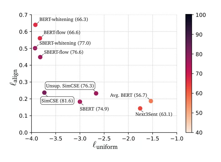
Figure 3: - plot of models based on BERT. Color of points and numbers in brackets represent average STS performance (Spearman’s correlation). Next3Sent: “next 3 sentences” from Table 2.
图 3:基于 BERT 的各模型的 - 图。点的颜色以及括号中的数字表示平均 STS 表现(Spearman 相关系数)。Next3Sent:表 2 中的“随后 3 句中的一句”。
Qualitative comparison.
定性比较。
We conduct a small-scale retrieval experiment using SBERT and SimCSE-BERT. We use 150k captions from Flickr30k dataset and take any random sentence as query to retrieve similar sentences (based on cosine similarity). As several examples shown in Table 8, the retrieved sentences by SimCSE have a higher quality compared to those retrieved by SBERT.
我们用 SBERT 和 SimCSE-BERT 做了一个小规模检索实验。我们使用 Flickr30k 中的 15 万条描述,随机取一句作为查询,按余弦相似度检索相似句子。如表 8 中的若干例子所示,SimCSE 检索到的句子质量高于 SBERT。
Table 8: Retrieved top-3 examples by SBERT and supervised SimCSE from Flickr30k (150k sentences).
| SBERT | Supervised SimCSE-BERT | |
|---|---|---|
| Query: A man riding a small boat in a harbor. | ||
| #1 | A group of men traveling over the ocean in a small boat. | A man on a moored blue and white boat. |
| #2 | Two men sit on the bow of a colorful boat. | A man is riding in a boat on the water. |
| #3 | A man wearing a life jacket is in a small boat on a lake. | A man in a blue boat on the water. |
| Query: A dog runs on the green grass near a wooden fence. | ||
| #1 | A dog runs on the green grass near a grove of trees. | The dog by the fence is running on the grass. |
| #2 | A brown and white dog runs through the green grass. | Dog running through grass in fenced area. |
| #3 | The dogs run in the green field. | A dog runs on the green grass near a grove of trees. |
表 8:SBERT 与有监督 SimCSE 从 Flickr30k(15 万句)中检索到的前 3 个例子。
| SBERT | 有监督 SimCSE-BERT | |
|---|---|---|
| 查询:A man riding a small boat in a harbor. | ||
| #1 | A group of men traveling over the ocean in a small boat. | A man on a moored blue and white boat. |
| #2 | Two men sit on the bow of a colorful boat. | A man is riding in a boat on the water. |
| #3 | A man wearing a life jacket is in a small boat on a lake. | A man in a blue boat on the water. |
| 查询:A dog runs on the green grass near a wooden fence. | ||
| #1 | A dog runs on the green grass near a grove of trees. | The dog by the fence is running on the grass. |
| #2 | A brown and white dog runs through the green grass. | Dog running through grass in fenced area. |
| #3 | The dogs run in the green field. | A dog runs on the green grass near a grove of trees. |
8 Related Work
8 相关工作
Early work in sentence embeddings builds upon the distributional hypothesis by predicting surrounding sentences of a given one (Kiros et al., 2015; Hill et al., 2016; Logeswaran and Lee, 2018). Pagliardini et al. (2018) show that simply augmenting the idea of word2vec (Mikolov et al., 2013) with n-gram embeddings leads to strong results. Several recent (and concurrent) approaches adopt contrastive objectives (Zhang et al., 2020; Giorgi et al., 2021; Wu et al., 2020; Meng et al., 2021; Carlsson et al., 2021; Kim et al., 2021; Yan et al., 2021) by taking different views—from data augmentation or different copies of models—of the same sentence or document. Compared to these work, SimCSE uses the simplest idea by taking different outputs of the same sentence from standard dropout, and performs the best on STS tasks.
早期的句子嵌入工作建立在分布假说之上,做法是预测给定句子的周围句子(Kiros et al., 2015; Hill et al., 2016; Logeswaran and Lee, 2018)。Pagliardini et al.(2018)表明,只需把 word2vec(Mikolov et al., 2013)的想法与 n-gram 嵌入结合起来,就能得到很强的结果。若干近期(以及同期)方法采用对比目标(Zhang et al., 2020; Giorgi et al., 2021; Wu et al., 2020; Meng et al., 2021; Carlsson et al., 2021; Kim et al., 2021; Yan et al., 2021),通过数据增广或模型的不同副本,对同一句子或文档构造不同视图。与这些工作相比,SimCSE 的想法最简单:只用标准 dropout 得到同一句子的不同输出,却在 STS 任务上取得了最好表现。
Supervised sentence embeddings are promised to have stronger performance compared to unsupervised counterparts. Conneau et al. (2017) propose to fine-tune a Siamese model on NLI datasets, which is further extended to other encoders or pre-trained models (Cer et al., 2018; Reimers and Gurevych, 2019). Furthermore, Wieting and Gimpel (2018); Wieting et al. (2020) demonstrate that bilingual and back-translation corpora provide useful supervision for learning semantic similarity. Another line of work focuses on regularizing embeddings (Li et al., 2020; Su et al., 2021; Huang et al., 2021) to alleviate the representation degeneration problem (as discussed in §5), and yields substantial improvement over pre-trained language models.
有监督句子嵌入理应比无监督方法有更强的表现。Conneau et al.(2017)提出在 NLI 数据集上微调孪生模型,这一做法后来被扩展到其他编码器或预训练模型(Cer et al., 2018; Reimers and Gurevych, 2019)。此外,Wieting and Gimpel(2018);Wieting et al.(2020)表明,双语和回译语料可以为学习语义相似度提供有用的监督。另一条线索则侧重对嵌入做正则(Li et al., 2020; Su et al., 2021; Huang et al., 2021),以缓解表示退化问题(见第 5 节的讨论),并在预训练语言模型上带来了可观提升。
9 Conclusion
9 结论
In this work, we propose SimCSE, a simple contrastive learning framework, which greatly improves state-of-the-art sentence embeddings on semantic textual similarity tasks. We present an unsupervised approach which predicts input sentence itself with dropout noise and a supervised approach utilizing NLI datasets. We further justify the inner workings of our approach by analyzing alignment and uniformity of SimCSE along with other baseline models. We believe that our contrastive objective, especially the unsupervised one, may have a broader application in NLP. It provides a new perspective on data augmentation with text input, and can be extended to other continuous representations and integrated in language model pre-training.
本文提出 SimCSE,这是一个简单的对比学习框架,在语义文本相似度任务上显著提升了句子嵌入的最好水平。我们给出一种用 dropout 噪声预测输入句子本身的无监督方法,以及一种利用 NLI 数据的有监督方法。我们还通过分析 SimCSE 与其他基线模型的对齐和均匀性,来说明这一方法的内在机制。我们认为,这一对比目标,尤其是无监督版本,在 NLP 中可能有更广的用途。它为文本输入上的数据增广提供了新的视角,也可以扩展到其他连续表示,并融入语言模型预训练。
Acknowledgements
致谢
We thank Tao Lei, Jason Lee, Zhengyan Zhang, Jinhyuk Lee, Alexander Wettig, Zexuan Zhong, and the members of the Princeton NLP group for helpful discussion and valuable feedback. This research is supported by a Graduate Fellowship at Princeton University and a gift award from Apple.
我们感谢 Tao Lei、Jason Lee、Zhengyan Zhang、Jinhyuk Lee、Alexander Wettig、Zexuan Zhong 以及 Princeton NLP 组的成员,感谢他们有益的讨论和宝贵的反馈。本研究得到 Princeton University 研究生奖学金以及 Apple 赠款的支持。
Appendix A Training Details
附录 A 训练细节
We implement SimCSE with transformers package (Wolf et al., 2020). For supervised SimCSE, we train our models for 3 epochs, evaluate the model every 250 training steps on the development set of STS-B and keep the best checkpoint for the final evaluation on test sets. We do the same for the unsupervised SimCSE, except that we train the model for one epoch. We carry out grid-search of batch size and learning rate on STS-B development set and adopt the hyperparameter settings in Table A.1. We find that SimCSE is not sensitive to batch sizes as long as tuning the learning rates accordingly, which contradicts the finding that contrastive learning requires large batch sizes (Chen et al., 2020). It is probably due to that all SimCSE models start from pre-trained checkpoints, which already provide us a good set of initial parameters.
我们用 transformers 工具包(Wolf et al., 2020)实现 SimCSE。对有监督 SimCSE,我们训练 3 个 epoch,每隔 250 个训练步在 STS-B 开发集上评估,并保留最好的检查点用于最终测试集评估。无监督 SimCSE 也采用同样做法,只是只训练 1 个 epoch。我们在 STS-B 开发集上对批量大小 和学习率 做网格搜索,并采用表 A.1 中的超参数设定。我们发现,只要相应地调整学习率,SimCSE 对批量大小并不敏感,这与对比学习需要大批量的发现并不一致(Chen et al., 2020)。这很可能是因为所有 SimCSE 模型都从预训练检查点出发,已经有了一组较好的初始参数。
Table A.1: Batch sizes and learning rates for SimCSE.
| Unsupervised | Supervised | |||||
|---|---|---|---|---|---|---|
| BERT | BERT | RoBERTa | RoBERTa | base | large | |
| base | large | base | large | |||
| Batch size | 64 | 64 | 512 | 512 | 512 | 512 |
| Learning rate | 3e-5 | 1e-5 | 1e-5 | 3e-5 | 5e-5 | 1e-5 |
表 A.1:SimCSE 的批量大小与学习率。
| 无监督 | 有监督 | |||||
|---|---|---|---|---|---|---|
| BERT | BERT | RoBERTa | RoBERTa | base | large | |
| base | large | base | large | |||
| 批量大小 | 64 | 64 | 512 | 512 | 512 | 512 |
| 学习率 | 3e-5 | 1e-5 | 1e-5 | 3e-5 | 5e-5 | 1e-5 |
For both unsupervised and supervised SimCSE, we take the [CLS] representation with an MLP layer on top of it as the sentence representation. Specially, for unsupervised SimCSE, we discard the MLP layer and only use the [CLS] output during test, since we find that it leads to better performance (ablation study in §6.3).
对无监督和有监督 SimCSE,我们都把带有上层 MLP 的 [CLS] 表示作为句子表示。特别地,对无监督 SimCSE,我们在测试时去掉 MLP,只使用 [CLS] 输出,因为我们发现这样效果更好(消融见第 6.3 节)。
Finally, we introduce one more optional variant which adds a masked language modeling (MLM) objective (Devlin et al., 2019) as an auxiliary loss to Eq. 1: ( is a hyperparameter). This helps SimCSE avoid catastrophic forgetting of token-level knowledge. As we will show in Table D.2, we find that adding this term can help improve performance on transfer tasks (not on sentence-level STS tasks).
最后,我们再引入一个可选变体:把掩码语言模型(MLM)目标(Devlin et al., 2019)作为辅助损失加到公式 1 上:( 是超参数)。这有助于 SimCSE 避免遗忘词元级知识。如表 D.2 所示,我们发现加入这一项有助于提升迁移任务上的表现(但不是句子级 STS 任务)。
Appendix B Different Settings for STS Evaluation
附录 B STS 评估的不同设定
We elaborate the differences in STS evaluation settings in previous work in terms of (a) whether to use additional regressors; (b) reported metrics; (c) different ways to aggregate results.
我们从以下几个方面说明以往工作中 STS 评估设定的差异:(a) 是否使用额外的回归器;(b) 所报告的指标;(c) 汇总结果的不同方式。
Additional regressors. The default SentEval implementation applies a linear regressor on top of frozen sentence embeddings for STS-B and SICK-R, and train the regressor on the training sets of the two tasks, while most sentence representation papers take the raw embeddings and evaluate in an unsupervised way. In our experiments, we do not apply any additional regressors and directly take cosine similarities for all STS tasks.
额外的回归器。SentEval 的默认实现会在冻结的句子嵌入之上,为 STS-B 和 SICK-R 再接一个线性回归器,并在这两个任务的训练集上训练该回归器;而大多数句子表示论文直接使用原始嵌入,以无监督方式评估。在我们的实验中,不加任何额外回归器,对所有 STS 任务都直接使用余弦相似度。
Metrics. Both Pearson’s and Spearman’s correlation coefficients are used in the literature. Reimers et al. (2016) argue that Spearman correlation, which measures the rankings instead of the actual scores, better suits the need of evaluating sentence embeddings. For all of our experiments, we report Spearman’s rank correlation.
指标。文献中既使用 Pearson 相关系数,也使用 Spearman 相关系数。Reimers et al.(2016)认为,Spearman 相关衡量的是排序而不是绝对分数,更适合评估句子嵌入。我们的全部实验都报告 Spearman 秩相关。
Aggregation methods. Given that each year’s STS challenge contains several subsets, there are different choices to gather results from them: one way is to concatenate all the topics and report the overall Spearman’s correlation (denoted as “all”), and the other is to calculate results for different subsets separately and average them (denoted as “mean” if it is simple average or “wmean” if weighted by the subset sizes). However, most papers do not claim the method they take, making it challenging for a fair comparison. We take some of the most recent work: SBERT (Reimers and Gurevych, 2019), BERT-flow (Li et al., 2020) and BERT-whitening (Su et al., 2021)[^12] as an example: In Table B.2, we compare our reproduced results to reported results of SBERT and BERT-whitening, and find that Reimers and Gurevych (2019) take the “all” setting but Li et al. (2020); Su et al. (2021) take the “wmean” setting, even though Li et al. (2020) claim that they take the same setting as Reimers and Gurevych (2019). Since the “all” setting fuses data from different topics together, it makes the evaluation closer to real-world scenarios, and unless specified, we take the “all” setting.
汇总方法。由于每年的 STS 挑战都包含若干子集,从中汇总结果有不同选择:一种是把所有主题拼接起来,报告总体的 Spearman 相关(记为 “all”);另一种是分别计算各子集的结果再取平均(简单平均记为 “mean”,按子集规模加权则记为 “wmean”)。然而,大多数论文并未说明采用了哪种方法,这给公平比较带来了困难。我们以若干近期工作为例:SBERT(Reimers and Gurevych, 2019)、BERT-flow(Li et al., 2020)和 BERT-whitening(Su et al., 2021)[^12]。在表 B.2 中,我们把复现结果与 SBERT 和 BERT-whitening 的报告结果相比较,发现 Reimers and Gurevych(2019)采用的是 “all” 设定,而 Li et al.(2020);Su et al.(2021)采用的是 “wmean” 设定,尽管 Li et al.(2020)声称他们采用了与 Reimers and Gurevych(2019)相同的设定。由于 “all” 设定把不同主题的数据融合在一起,评估更接近真实场景;除非另有说明,我们采用 “all” 设定。
[^12]: Li et al. (2020) and Su et al. (2021) have consistent results, so we assume that they take the same evaluation and just take BERT-whitening in experiments here.
[^12]: Li et al.(2020)与 Su et al.(2021)的结果一致,因此我们假定他们采用了相同的评估,并在这里的实验中只取 BERT-whitening。
We list evaluation settings for a number of previous work in Table B.1. Some of the settings are reported by the paper and some of them are inferred by comparing the results and checking their code. As we can see, the evaluation protocols are very incoherent across different papers. We call for unifying the setting in evaluating sentence embeddings for future research. We will also release our evaluation code for better reproducibility. Since previous work uses different evaluation protocols from ours, we further evaluate our models in these settings to make a direct comparison to the published numbers. We evaluate SimCSE with “wmean” and Spearman’s correlation to directly compare to Li et al. (2020) and Su et al. (2021) in Table B.3.
我们在表 B.1 中列出了若干以往工作的评估设定。其中一些由论文明确报告,另一些则是通过比较结果并检查其代码推断出来的。可以看到,不同论文的评估协议非常不一致。我们呼吁后续研究在句子嵌入评估中统一设定。我们也将发布评估代码,以便更好地复现。由于以往工作使用的评估协议与我们不同,我们还在这些设定下进一步评估了自己的模型,以便与已发表数字直接比较。我们用 “wmean” 和 Spearman 相关评估 SimCSE,以便在表 B.3 中与 Li et al.(2020)和 Su et al.(2021)直接比较。
Table B.1: STS evaluation protocols used in different papers. “Reg.”: whether an additional regressor is used; “aggr.”: methods to aggregate different subset results.
| Paper | Reg. | Metric | Aggr. |
|---|---|---|---|
| Hill et al. (2016) | Both | all | |
| Conneau et al. (2017) | ✓ | Pearson | mean |
| Conneau and Kiela (2018) | ✓ | Pearson | mean |
| Reimers and Gurevych (2019) | Spearman | all | |
| Zhang et al. (2020) | Spearman | all | |
| Li et al. (2020) | Spearman | wmean | |
| Su et al. (2021) | Spearman | wmean | |
| Wieting et al. (2020) | Pearson | mean | |
| Giorgi et al. (2021) | Spearman | mean | |
| Ours | Spearman | all |
表 B.1:不同论文使用的 STS 评估协议。 “Reg.”:是否使用额外的回归器;“aggr.”:汇总不同子集结果的方法。
| 论文 | Reg. | 指标 | 汇总 |
|---|---|---|---|
| Hill et al. (2016) | Both | all | |
| Conneau et al. (2017) | ✓ | Pearson | mean |
| Conneau and Kiela (2018) | ✓ | Pearson | mean |
| Reimers and Gurevych (2019) | Spearman | all | |
| Zhang et al. (2020) | Spearman | all | |
| Li et al. (2020) | Spearman | wmean | |
| Su et al. (2021) | Spearman | wmean | |
| Wieting et al. (2020) | Pearson | mean | |
| Giorgi et al. (2021) | Spearman | mean | |
| 本文 | Spearman | all |
Table B.2: Comparisons of our reproduced results using different evaluation protocols and the original numbers. ♣: results from Reimers and Gurevych (2019); ♠: results from Su et al. (2021); Other results are reproduced by us. From the table we see that SBERT takes the “all” evaluation and BERT-whitening takes the “wmean” evaluation.
| Model | STS12 | STS13 | STS14 | STS15 | STS16 | STS-B | SICK-R | Avg. |
|---|---|---|---|---|---|---|---|---|
| SBERT (all) | 70.97 | 76.53 | 73.19 | 79.09 | 74.30 | 76.98 | 72.91 | 74.85 |
| SBERT (wmean) | 66.35 | 73.76 | 73.88 | 77.33 | 73.62 | 76.98 | 72.91 | 73.55 |
| SBERT♣ | 70.97 | 76.53 | 73.19 | 79.09 | 74.30 | 77.03 | 72.91 | 74.89 |
| BERT-whitening (NLI, all) | 57.83 | 66.90 | 60.89 | 75.08 | 71.30 | 68.23 | 63.73 | 66.28 |
| BERT-whitening (NLI, wmean) | 61.43 | 65.90 | 65.96 | 74.80 | 73.10 | 68.23 | 63.73 | 67.59 |
| BERT-whitening (NLI)♠ | 61.69 | 65.70 | 66.02 | 75.11 | 73.11 | 68.19 | 63.60 | 67.63 |
| BERT-whitening (target, all) | 42.88 | 77.77 | 66.27 | 63.60 | 67.58 | 71.34 | 60.40 | 64.26 |
| BERT-whitening (target, wmean) | 63.38 | 73.01 | 69.13 | 74.48 | 72.56 | 71.34 | 60.40 | 69.19 |
| BERT-whitening (target)♠ | 63.62 | 73.02 | 69.23 | 74.52 | 72.15 | 71.34 | 60.60 | 69.21 |
表 B.2:用不同评估协议复现的结果与原始数字的比较。 ♣:结果来自 Reimers and Gurevych(2019);♠:结果来自 Su et al.(2021);其余结果由我们复现。从表中可以看出,SBERT 采用 “all” 评估,BERT-whitening 采用 “wmean” 评估。
| Model | STS12 | STS13 | STS14 | STS15 | STS16 | STS-B | SICK-R | Avg. |
|---|---|---|---|---|---|---|---|---|
| SBERT (all) | 70.97 | 76.53 | 73.19 | 79.09 | 74.30 | 76.98 | 72.91 | 74.85 |
| SBERT (wmean) | 66.35 | 73.76 | 73.88 | 77.33 | 73.62 | 76.98 | 72.91 | 73.55 |
| SBERT♣ | 70.97 | 76.53 | 73.19 | 79.09 | 74.30 | 77.03 | 72.91 | 74.89 |
| BERT-whitening (NLI, all) | 57.83 | 66.90 | 60.89 | 75.08 | 71.30 | 68.23 | 63.73 | 66.28 |
| BERT-whitening (NLI, wmean) | 61.43 | 65.90 | 65.96 | 74.80 | 73.10 | 68.23 | 63.73 | 67.59 |
| BERT-whitening (NLI)♠ | 61.69 | 65.70 | 66.02 | 75.11 | 73.11 | 68.19 | 63.60 | 67.63 |
| BERT-whitening (target, all) | 42.88 | 77.77 | 66.27 | 63.60 | 67.58 | 71.34 | 60.40 | 64.26 |
| BERT-whitening (target, wmean) | 63.38 | 73.01 | 69.13 | 74.48 | 72.56 | 71.34 | 60.40 | 69.19 |
| BERT-whitening (target)♠ | 63.62 | 73.02 | 69.23 | 74.52 | 72.15 | 71.34 | 60.60 | 69.21 |
Table B.3: STS results with “wmean” setting (Spearman). ♠: from Li et al. (2020); Su et al. (2021).
| Model | STS12 | STS13 | STS14 | STS15 | STS16 | STS-B | SICK-R | Avg. |
|---|---|---|---|---|---|---|---|---|
| BERT (first-last avg.)♠ | 57.86 | 61.97 | 62.49 | 70.96 | 69.76 | 59.04 | 63.75 | 63.69 |
| + flow (NLI)♠ | 59.54 | 64.69 | 64.66 | 72.92 | 71.84 | 58.56 | 65.44 | 65.38 |
| + flow (target)♠ | 63.48 | 72.14 | 68.42 | 73.77 | 75.37 | 70.72 | 63.11 | 69.57 |
| + whitening (NLI)♠ | 61.69 | 65.70 | 66.02 | 75.11 | 73.11 | 68.19 | 63.60 | 67.63 |
| + whitening (target)♠ | 63.62 | 73.02 | 69.23 | 74.52 | 72.15 | 71.34 | 60.60 | 69.21 |
| ∗Unsup. SimCSE-BERT | 70.14 | 79.56 | 75.91 | 81.46 | 79.07 | 76.85 | 72.23 | 76.46 |
| SBERT (first-last avg.)♠ | 68.70 | 74.37 | 74.73 | 79.65 | 75.21 | 77.63 | 74.84 | 75.02 |
| + flow (NLI)♠ | 67.75 | 76.73 | 75.53 | 80.63 | 77.58 | 79.10 | 78.03 | 76.48 |
| + flow (target)♠ | 68.95 | 78.48 | 77.62 | 81.95 | 78.94 | 81.03 | 74.97 | 77.42 |
| + whitening (NLI)♠ | 69.11 | 75.79 | 75.76 | 82.31 | 79.61 | 78.66 | 76.33 | 76.80 |
| + whitening (target)♠ | 69.01 | 78.10 | 77.04 | 80.83 | 77.93 | 80.50 | 72.54 | 76.56 |
| ∗Sup. SimCSE-BERT | 70.90 | 81.49 | 80.19 | 83.79 | 81.89 | 84.25 | 80.39 | 80.41 |
表 B.3:“wmean” 设定下的 STS 结果(Spearman)。 ♠:来自 Li et al.(2020);Su et al.(2021)。
| Model | STS12 | STS13 | STS14 | STS15 | STS16 | STS-B | SICK-R | Avg. |
|---|---|---|---|---|---|---|---|---|
| BERT (first-last avg.)♠ | 57.86 | 61.97 | 62.49 | 70.96 | 69.76 | 59.04 | 63.75 | 63.69 |
| + flow (NLI)♠ | 59.54 | 64.69 | 64.66 | 72.92 | 71.84 | 58.56 | 65.44 | 65.38 |
| + flow (target)♠ | 63.48 | 72.14 | 68.42 | 73.77 | 75.37 | 70.72 | 63.11 | 69.57 |
| + whitening (NLI)♠ | 61.69 | 65.70 | 66.02 | 75.11 | 73.11 | 68.19 | 63.60 | 67.63 |
| + whitening (target)♠ | 63.62 | 73.02 | 69.23 | 74.52 | 72.15 | 71.34 | 60.60 | 69.21 |
| ∗Unsup. SimCSE-BERT | 70.14 | 79.56 | 75.91 | 81.46 | 79.07 | 76.85 | 72.23 | 76.46 |
| SBERT (first-last avg.)♠ | 68.70 | 74.37 | 74.73 | 79.65 | 75.21 | 77.63 | 74.84 | 75.02 |
| + flow (NLI)♠ | 67.75 | 76.73 | 75.53 | 80.63 | 77.58 | 79.10 | 78.03 | 76.48 |
| + flow (target)♠ | 68.95 | 78.48 | 77.62 | 81.95 | 78.94 | 81.03 | 74.97 | 77.42 |
| + whitening (NLI)♠ | 69.11 | 75.79 | 75.76 | 82.31 | 79.61 | 78.66 | 76.33 | 76.80 |
| + whitening (target)♠ | 69.01 | 78.10 | 77.04 | 80.83 | 77.93 | 80.50 | 72.54 | 76.56 |
| ∗Sup. SimCSE-BERT | 70.90 | 81.49 | 80.19 | 83.79 | 81.89 | 84.25 | 80.39 | 80.41 |
Appendix C Baseline Models
附录 C 基线模型
We elaborate on how we obtain different baselines for comparison in our experiments:
我们说明实验中用于比较的各基线是如何得到的:
- For average GloVe embedding (Pennington et al., 2014), InferSent (Conneau et al., 2017) and Universal Sentence Encoder (Cer et al., 2018), we directly report the results from Reimers and Gurevych (2019), since our evaluation setting is the same as theirs.
- 对平均 GloVe 嵌入(Pennington et al., 2014)、InferSent(Conneau et al., 2017)以及 Universal Sentence Encoder(Cer et al., 2018),我们直接报告 Reimers and Gurevych(2019)的结果,因为我们的评估设定与他们相同。
- For BERT (Devlin et al., 2019) and RoBERTa (Liu et al., 2019), we download the pre-trained model weights from HuggingFace’s Transformers[^13], and evaluate the models with our own scripts.
- 对 BERT(Devlin et al., 2019)和 RoBERTa(Liu et al., 2019),我们从 HuggingFace 的 Transformers[^13] 下载预训练模型权重,并用自己的脚本评估。
- For SBERT and SRoBERTa (Reimers and Gurevych, 2019), we reuse the results from the original paper. For results not reported by Reimers and Gurevych (2019), such as the performance of SRoBERTa on transfer tasks, we download the model weights from SentenceTransformers[^14] and evaluate them.
- 对 SBERT 和 SRoBERTa(Reimers and Gurevych, 2019),我们沿用原论文的结果。对 Reimers and Gurevych(2019)未报告的结果,例如 SRoBERTa 在迁移任务上的表现,我们从 SentenceTransformers[^14] 下载模型权重并自行评估。
- For DeCLUTR (Giorgi et al., 2021) and contrastive tension (Carlsson et al., 2021), we reevaluate their checkpoints in our setting.
- 对 DeCLUTR(Giorgi et al., 2021)和 contrastive tension(Carlsson et al., 2021),我们在自己的设定下重新评估了它们的检查点。
- For BERT-flow (Li et al., 2020), since their original numbers take a different setting, we retrain their models using their code[^15], and evaluate the models using our own script.
- 对 BERT-flow(Li et al., 2020),由于其原始数字采用了不同设定,我们用他们的代码[^15]重新训练模型,并用自己的脚本评估。
- For BERT-whitening (Su et al., 2021), we implemented our own version of whitening script following the same pooling method in Su et al. (2021), i.e. first-last average pooling. Our implementation can reproduce the results from the original paper (see Table B.2).
- 对 BERT-whitening(Su et al., 2021),我们按照 Su et al.(2021)相同的池化方法(即 first-last 平均池化)实现了自己的 whitening 脚本。我们的实现能够复现原论文的结果(见表 B.2)。
For both BERT-flow and BERT-whitening, they have two variants of postprocessing: one takes the NLI data (“NLI”) and one directly learns the embedding distribution on the target sets (“target”). We find that in our evaluation setting, “target” is generally worse than “NLI” (Table C.1), so we only report the NLI variant in the main results.
对 BERT-flow 和 BERT-whitening,后处理都有两个变体:一个使用 NLI 数据(“NLI”),一个直接在目标集上学习嵌入分布(“target”)。我们发现,在我们的评估设定下,“target” 总体上不如 “NLI”(表 C.1),因此在主要结果中只报告 NLI 变体。
Table C.1: Comparison of using NLI or target data for postprocessing methods (“all”, Spearman’s correlation).
| Model | STS12 | STS13 | STS14 | STS15 | STS16 | STS-B | SICK-R | Avg. |
|---|---|---|---|---|---|---|---|---|
| BERT-flow (NLI) | 58.40 | 67.10 | 60.85 | 75.16 | 71.22 | 68.66 | 64.47 | 66.55 |
| BERT-flow (target) | 53.15 | 78.38 | 66.02 | 62.09 | 70.84 | 71.70 | 61.97 | 66.31 |
| BERT-whitening (NLI) | 57.83 | 66.90 | 60.90 | 75.08 | 71.31 | 68.24 | 63.73 | 66.28 |
| BERT-whitening (target) | 42.88 | 77.77 | 66.28 | 63.60 | 67.58 | 71.34 | 60.40 | 64.26 |
| SBERT-flow (NLI) | 69.78 | 77.27 | 74.35 | 82.01 | 77.46 | 79.12 | 76.21 | 76.60 |
| SBERT-flow (target) | 66.18 | 82.69 | 76.22 | 73.72 | 75.71 | 79.99 | 73.82 | 75.48 |
| SBERT-whitening (NLI) | 69.65 | 77.57 | 74.66 | 82.27 | 78.39 | 79.52 | 76.91 | 77.00 |
| SBERT-whitening (target) | 52.91 | 81.91 | 75.44 | 72.24 | 72.93 | 80.50 | 72.54 | 72.64 |
表 C.1:后处理方法使用 NLI 或目标数据的比较(“all”,Spearman 相关系数)。
| Model | STS12 | STS13 | STS14 | STS15 | STS16 | STS-B | SICK-R | Avg. |
|---|---|---|---|---|---|---|---|---|
| BERT-flow (NLI) | 58.40 | 67.10 | 60.85 | 75.16 | 71.22 | 68.66 | 64.47 | 66.55 |
| BERT-flow (target) | 53.15 | 78.38 | 66.02 | 62.09 | 70.84 | 71.70 | 61.97 | 66.31 |
| BERT-whitening (NLI) | 57.83 | 66.90 | 60.90 | 75.08 | 71.31 | 68.24 | 63.73 | 66.28 |
| BERT-whitening (target) | 42.88 | 77.77 | 66.28 | 63.60 | 67.58 | 71.34 | 60.40 | 64.26 |
| SBERT-flow (NLI) | 69.78 | 77.27 | 74.35 | 82.01 | 77.46 | 79.12 | 76.21 | 76.60 |
| SBERT-flow (target) | 66.18 | 82.69 | 76.22 | 73.72 | 75.71 | 79.99 | 73.82 | 75.48 |
| SBERT-whitening (NLI) | 69.65 | 77.57 | 74.66 | 82.27 | 78.39 | 79.52 | 76.91 | 77.00 |
| SBERT-whitening (target) | 52.91 | 81.91 | 75.44 | 72.24 | 72.93 | 80.50 | 72.54 | 72.64 |
Appendix D Ablation Studies
附录 D 消融实验
Normalization and temperature.
归一化与温度。
We train SimCSE using both dot product and cosine similarity with different temperatures and evaluate them on the STS-B development set. As shown in Table D.1, with a carefully tuned temperature , cosine similarity is better than dot product.
我们分别用点积和余弦相似度、并配合不同温度训练 SimCSE,在 STS-B 开发集上评估。如表 D.1 所示,在仔细调好温度 后,余弦相似度优于点积。
Table D.1: STS-B development results (Spearman’s correlation) with different temperatures. “N/A”: Dot product instead of cosine similarity.
| N/A | 0.001 | 0.01 | 0.05 | 0.1 | 1 | |
|---|---|---|---|---|---|---|
| STS-B | 85.9 | 84.9 | 85.4 | 86.2 | 82.0 | 64.0 |
表 D.1:不同温度在 STS-B 开发集上的结果(Spearman 相关系数)。 “N/A”:使用点积而不是余弦相似度。
| N/A | 0.001 | 0.01 | 0.05 | 0.1 | 1 | |
|---|---|---|---|---|---|---|
| STS-B | 85.9 | 84.9 | 85.4 | 86.2 | 82.0 | 64.0 |
MLM auxiliary task.
MLM 辅助任务。
Finally, we study the impact of the MLM auxiliary objective with different . As shown in Table D.2, the token-level MLM objective improves the averaged performance on transfer tasks modestly, yet it brings a consistent drop in semantic textual similarity tasks.
最后,我们考察不同 下 MLM 辅助目标的影响。如表 D.2 所示,词元级 MLM 目标对迁移任务的平均表现有小幅提升,但会在语义文本相似度任务上带来一贯的下降。
Table D.2: Ablation studies of the MLM objective based on the development sets using BERT.
| Model | STS-B | Avg. transfer |
|---|---|---|
| w/o MLM | 86.2 | 85.8 |
| w/ MLM, | 85.7 | 86.1 |
| w/ MLM, | 85.7 | 86.2 |
| w/ MLM, | 85.1 | 85.8 |
表 D.2:基于开发集、使用 BERT 的 MLM 目标消融。
| 模型 | STS-B | 平均迁移 |
|---|---|---|
| 不加 MLM | 86.2 | 85.8 |
| 加 MLM, | 85.7 | 86.1 |
| 加 MLM, | 85.7 | 86.2 |
| 加 MLM, | 85.1 | 85.8 |
Appendix E Transfer Tasks
附录 E 迁移任务
We evaluate our models on the following transfer tasks: MR (Pang and Lee, 2005), CR (Hu and Liu, 2004), SUBJ (Pang and Lee, 2004), MPQA (Wiebe et al., 2005), SST-2 (Socher et al., 2013), TREC (Voorhees and Tice, 2000) and MRPC (Dolan and Brockett, 2005). A logistic regression classifier is trained on top of (frozen) sentence embeddings produced by different methods. We follow default configurations from SentEval[^16].
我们在下列迁移任务上评估模型:MR(Pang and Lee, 2005)、CR(Hu and Liu, 2004)、SUBJ(Pang and Lee, 2004)、MPQA(Wiebe et al., 2005)、SST-2(Socher et al., 2013)、TREC(Voorhees and Tice, 2000)以及 MRPC(Dolan and Brockett, 2005)。在不同方法得到的(冻结)句子嵌入之上训练一个逻辑回归分类器。我们沿用 SentEval 的默认配置[^16]。
Table E.1 shows the evaluation results on transfer tasks. We find that supervised SimCSE performs on par or better than previous approaches, although the trend of unsupervised models remains unclear. We find that adding this MLM term consistently improves performance on transfer tasks, confirming our intuition that sentence-level objective may not directly benefit transfer tasks. We also experiment with post-processing methods (BERT-flow/whitening) and find that they both hurt performance compared to their base models, showing that good uniformity of representations does not lead to better embeddings for transfer learning. As we argued earlier, we think that transfer tasks are not a major goal for sentence embeddings, and thus we take the STS results for main comparison.
表 E.1 给出了迁移任务上的评估结果。我们发现,有监督 SimCSE 的表现与以往方法持平或更好,但无监督模型的趋势仍不清晰。我们发现,加入这一 MLM 项会一贯提升迁移任务上的表现,这印证了我们的直觉:句子级目标未必能直接惠及迁移任务。我们还试验了后处理方法(BERT-flow/whitening),发现它们相对各自的基础模型都会损害表现,说明表示具有良好的均匀性,并不意味着在迁移学习上会得到更好的嵌入。正如前文所述,我们认为迁移任务并不是句子嵌入的主要目标,因此以 STS 结果作为主要比较。
Table E.1: Transfer task results of different sentence embedding models (measured as accuracy). ♣: results from Reimers and Gurevych (2019); ♥: results from Zhang et al. (2020). We highlight the highest numbers among models with the same pre-trained encoder. MLM: adding MLM as an auxiliary task with .
| Model | MR | CR | SUBJ | MPQA | SST | TREC | MRPC | Avg. |
|---|---|---|---|---|---|---|---|---|
| Unsupervised models | ||||||||
| GloVe embeddings (avg.)♣ | 77.25 | 78.30 | 91.17 | 87.85 | 80.18 | 83.00 | 72.87 | 81.52 |
| Skip-thought♥ | 76.50 | 80.10 | 93.60 | 87.10 | 82.00 | 92.20 | 73.00 | 83.50 |
| Avg. BERT embeddings♣ | 78.66 | 86.25 | 94.37 | 88.66 | 84.40 | 92.80 | 69.54 | 84.94 |
| BERT-[CLS] embedding♣ | 78.68 | 84.85 | 94.21 | 88.23 | 84.13 | 91.40 | 71.13 | 84.66 |
| IS-BERT♥ | 81.09 | 87.18 | 94.96 | 88.75 | 85.96 | 88.64 | 74.24 | 85.83 |
| ∗SimCSE-BERT | 81.18 | 86.46 | 94.45 | 88.88 | 85.50 | 89.80 | 74.43 | 85.81 |
| w/ MLM | 82.92 | 87.23 | 95.71 | 88.73 | 86.81 | 87.01 | 78.07 | 86.64 |
| ∗SimCSE-RoBERTa | 81.04 | 87.74 | 93.28 | 86.94 | 86.60 | 84.60 | 73.68 | 84.84 |
| w/ MLM | 83.37 | 87.76 | 95.05 | 87.16 | 89.02 | 90.80 | 75.13 | 86.90 |
| ∗SimCSE-RoBERTa | 82.74 | 87.87 | 93.66 | 88.22 | 88.58 | 92.00 | 69.68 | 86.11 |
| w/ MLM | 84.66 | 88.56 | 95.43 | 87.50 | 89.46 | 95.00 | 72.41 | 87.57 |
| Supervised models | ||||||||
| InferSent-GloVe♣ | 81.57 | 86.54 | 92.50 | 90.38 | 84.18 | 88.20 | 75.77 | 85.59 |
| Universal Sentence Encoder♣ | 80.09 | 85.19 | 93.98 | 86.70 | 86.38 | 93.20 | 70.14 | 85.10 |
| SBERT♣ | 83.64 | 89.43 | 94.39 | 89.86 | 88.96 | 89.60 | 76.00 | 87.41 |
| ∗SimCSE-BERT | 82.69 | 89.25 | 94.81 | 89.59 | 87.31 | 88.40 | 73.51 | 86.51 |
| w/ MLM | 82.68 | 88.88 | 94.52 | 89.82 | 88.41 | 87.60 | 76.12 | 86.86 |
| SRoBERTa | 84.91 | 90.83 | 92.56 | 88.75 | 90.50 | 88.60 | 78.14 | 87.76 |
| ∗SimCSE-RoBERTa | 84.92 | 92.00 | 94.11 | 89.82 | 91.27 | 88.80 | 75.65 | 88.08 |
| w/ MLM | 85.08 | 91.76 | 94.02 | 89.72 | 92.31 | 91.20 | 76.52 | 88.66 |
| ∗SimCSE-RoBERTa | 88.12 | 92.37 | 95.11 | 90.49 | 92.75 | 91.80 | 76.64 | 89.61 |
| w/ MLM | 88.45 | 92.53 | 95.19 | 90.58 | 93.30 | 93.80 | 77.74 | 90.23 |
表 E.1:不同句子嵌入模型在迁移任务上的结果(以准确率衡量)。 ♣:结果来自 Reimers and Gurevych(2019);♥:结果来自 Zhang et al.(2020)。我们在使用同一预训练编码器的模型中标出最高数字。MLM:把 MLM 作为辅助任务加入,且 。
| 模型 | MR | CR | SUBJ | MPQA | SST | TREC | MRPC | Avg. |
|---|---|---|---|---|---|---|---|---|
| 无监督模型 | ||||||||
| GloVe embeddings (avg.)♣ | 77.25 | 78.30 | 91.17 | 87.85 | 80.18 | 83.00 | 72.87 | 81.52 |
| Skip-thought♥ | 76.50 | 80.10 | 93.60 | 87.10 | 82.00 | 92.20 | 73.00 | 83.50 |
| Avg. BERT embeddings♣ | 78.66 | 86.25 | 94.37 | 88.66 | 84.40 | 92.80 | 69.54 | 84.94 |
| BERT-[CLS] embedding♣ | 78.68 | 84.85 | 94.21 | 88.23 | 84.13 | 91.40 | 71.13 | 84.66 |
| IS-BERT♥ | 81.09 | 87.18 | 94.96 | 88.75 | 85.96 | 88.64 | 74.24 | 85.83 |
| ∗SimCSE-BERT | 81.18 | 86.46 | 94.45 | 88.88 | 85.50 | 89.80 | 74.43 | 85.81 |
| w/ MLM | 82.92 | 87.23 | 95.71 | 88.73 | 86.81 | 87.01 | 78.07 | 86.64 |
| ∗SimCSE-RoBERTa | 81.04 | 87.74 | 93.28 | 86.94 | 86.60 | 84.60 | 73.68 | 84.84 |
| w/ MLM | 83.37 | 87.76 | 95.05 | 87.16 | 89.02 | 90.80 | 75.13 | 86.90 |
| ∗SimCSE-RoBERTa | 82.74 | 87.87 | 93.66 | 88.22 | 88.58 | 92.00 | 69.68 | 86.11 |
| w/ MLM | 84.66 | 88.56 | 95.43 | 87.50 | 89.46 | 95.00 | 72.41 | 87.57 |
| 有监督模型 | ||||||||
| InferSent-GloVe♣ | 81.57 | 86.54 | 92.50 | 90.38 | 84.18 | 88.20 | 75.77 | 85.59 |
| Universal Sentence Encoder♣ | 80.09 | 85.19 | 93.98 | 86.70 | 86.38 | 93.20 | 70.14 | 85.10 |
| SBERT♣ | 83.64 | 89.43 | 94.39 | 89.86 | 88.96 | 89.60 | 76.00 | 87.41 |
| ∗SimCSE-BERT | 82.69 | 89.25 | 94.81 | 89.59 | 87.31 | 88.40 | 73.51 | 86.51 |
| w/ MLM | 82.68 | 88.88 | 94.52 | 89.82 | 88.41 | 87.60 | 76.12 | 86.86 |
| SRoBERTa | 84.91 | 90.83 | 92.56 | 88.75 | 90.50 | 88.60 | 78.14 | 87.76 |
| ∗SimCSE-RoBERTa | 84.92 | 92.00 | 94.11 | 89.82 | 91.27 | 88.80 | 75.65 | 88.08 |
| w/ MLM | 85.08 | 91.76 | 94.02 | 89.72 | 92.31 | 91.20 | 76.52 | 88.66 |
| ∗SimCSE-RoBERTa | 88.12 | 92.37 | 95.11 | 90.49 | 92.75 | 91.80 | 76.64 | 89.61 |
| w/ MLM | 88.45 | 92.53 | 95.19 | 90.58 | 93.30 | 93.80 | 77.74 | 90.23 |
Appendix F Distribution of Singular Values
附录 F 奇异值分布
Figure F.1 shows the singular value distribution of SimCSE together with other baselines. For both unsupervised and supervised cases, singular value drops the fastest for vanilla BERT or SBERT embeddings, while SimCSE helps flatten the spectrum distribution. Postprocessing-based methods such as BERT-flow or BERT-whitening flatten the curve even more since they directly aim for the goal of mapping embeddings to an isotropic distribution.
图 F.1 给出了 SimCSE 以及其他基线的奇异值分布。无论是无监督还是有监督情形,原始 BERT 或 SBERT 嵌入的奇异值下降都最快,而 SimCSE 有助于把谱分布压得更平。BERT-flow 或 BERT-whitening 这类基于后处理的方法会把曲线压得更平,因为它们直接以把嵌入映射到各向同性分布为目标。
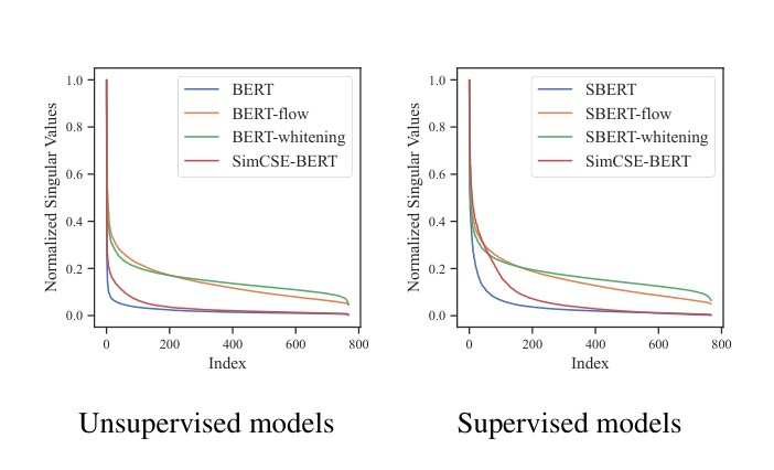
Figure F.1: Singular value distributions of sentence embedding matrix from sentences in STS-B. We normalize the singular values so that the largest one is 1.
图 F.1:来自 STS-B 句子的句子嵌入矩阵的奇异值分布。我们将奇异值归一化,使最大值为 1。
Appendix G Cosine-similarity Distribution
附录 G 余弦相似度分布
To directly show the strengths of our approaches on STS tasks, we illustrate the cosine similarity distributions of STS-B pairs with different groups of human ratings in Figure G.1. Compared to all the baseline models, both unsupervised and supervised SimCSE better distinguish sentence pairs with different levels of similarities, thus leading to a better performance on STS tasks. In addition, we observe that SimCSE generally shows a more scattered distribution than BERT or SBERT, but also preserves a lower variance on semantically similar sentence pairs compared to whitened distribution. This observation further validates that SimCSE can achieve a better alignment-uniformity balance.
为了直接展示我们的方法在 STS 任务上的优势,我们在图 G.1 中给出了不同人工评分组别下 STS-B 句子对的余弦相似度分布。与所有基线模型相比,无监督和有监督 SimCSE 都能更好地区分不同相似程度的句子对,从而在 STS 任务上取得更好表现。此外我们观察到,与 BERT 或 SBERT 相比,SimCSE 的分布通常更分散,但在语义相近的句子对上,方差又低于 whitening 后的分布。这一观察进一步印证:SimCSE 能够在对齐与均匀性之间取得更好的平衡。
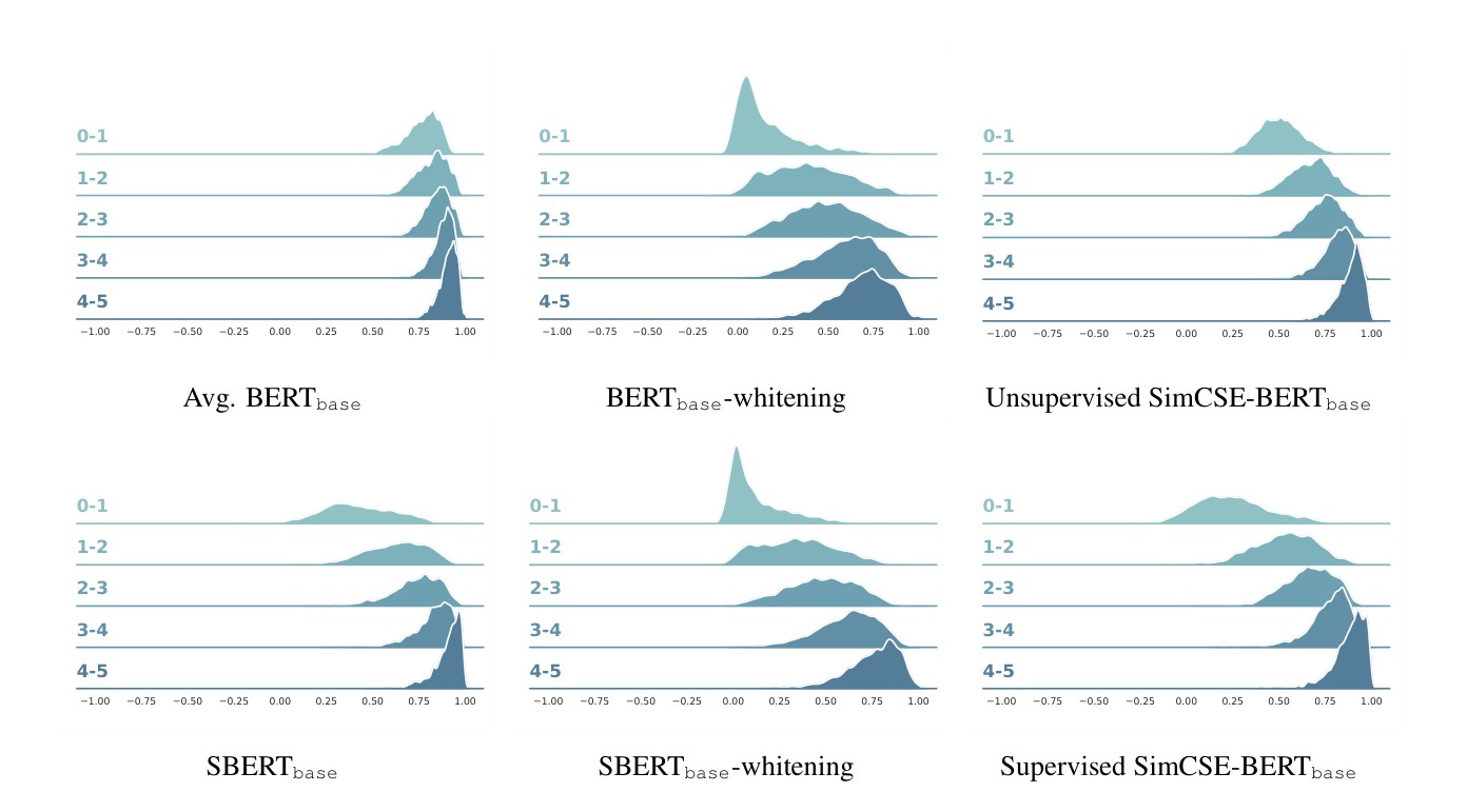
Figure G.1: Density plots of cosine similarities between sentence pairs in STS-B. Pairs are divided into 5 groups based on ground truth ratings (higher means more similar) along the y-axis, and x-axis is the cosine similarity.
图 G.1:STS-B 中句子对余弦相似度的密度图。句子对按真实评分分成 5 组(越高表示越相似),沿 y 轴排列;x 轴为余弦相似度。
References
参考文献
Eneko Agirre, Carmen Banea, Claire Cardie, Daniel Cer, Mona Diab, Aitor Gonzalez-Agirre, Weiwei Guo, Iñigo Lopez-Gazpio, Montse Maritxalar, Rada Mihalcea, German Rigau, Larraitz Uria, and Janyce Wiebe. 2015. SemEval-2015 task 2: Semantic textual similarity, English, Spanish and pilot on interpretability. In Proceedings of the 9th International Workshop on Semantic Evaluation (SemEval 2015), pages 252–263.
Eneko Agirre, Carmen Banea, Claire Cardie, Daniel Cer, Mona Diab, Aitor Gonzalez-Agirre, Weiwei Guo, Rada Mihalcea, German Rigau, and Janyce Wiebe. 2014. SemEval-2014 task 10: Multilingual semantic textual similarity. In Proceedings of the 8th International Workshop on Semantic Evaluation (SemEval 2014), pages 81–91.
Eneko Agirre, Carmen Banea, Daniel Cer, Mona Diab, Aitor Gonzalez-Agirre, Rada Mihalcea, German Rigau, and Janyce Wiebe. 2016. SemEval-2016 task 1: Semantic textual similarity, monolingual and cross-lingual evaluation. In Proceedings of the 10th International Workshop on Semantic Evaluation (SemEval-2016), pages 497–511. Association for Computational Linguistics.
Eneko Agirre, Daniel Cer, Mona Diab, and Aitor Gonzalez-Agirre. 2012. SemEval-2012 task 6: A pilot on semantic textual similarity. In *SEM 2012: The First Joint Conference on Lexical and Computational Semantics – Volume 1: Proceedings of the main conference and the shared task, and Volume 2: Proceedings of the Sixth International Workshop on Semantic Evaluation (SemEval 2012), pages 385–393.
Eneko Agirre, Daniel Cer, Mona Diab, Aitor Gonzalez-Agirre, and Weiwei Guo. 2013. *SEM 2013 shared task: Semantic textual similarity. In Second Joint Conference on Lexical and Computational Semantics (*SEM), Volume 1: Proceedings of the Main Conference and the Shared Task: Semantic Textual Similarity, pages 32–43.
Sanjeev Arora, Yingyu Liang, and Tengyu Ma. 2017. A simple but tough-to-beat baseline for sentence embeddings. In International Conference on Learning Representations (ICLR).
Samuel R. Bowman, Gabor Angeli, Christopher Potts, and Christopher D. Manning. 2015. A large annotated corpus for learning natural language inference. In Empirical Methods in Natural Language Processing (EMNLP), pages 632–642.
Fredrik Carlsson, Amaru Cuba Gyllensten, Evangelia Gogoulou, Erik Ylipää Hellqvist, and Magnus Sahlgren. 2021. Semantic re-tuning with contrastive tension. In International Conference on Learning Representations (ICLR).
Daniel Cer, Mona Diab, Eneko Agirre, Iñigo Lopez-Gazpio, and Lucia Specia. 2017. SemEval-2017 task 1: Semantic textual similarity multilingual and crosslingual focused evaluation. In Proceedings of the 11th International Workshop on Semantic Evaluation (SemEval-2017), pages 1–14.
Daniel Cer, Yinfei Yang, Sheng-yi Kong, Nan Hua, Nicole Limtiaco, Rhomni St. John, Noah Constant, Mario Guajardo-Cespedes, Steve Yuan, Chris Tar, Brian Strope, and Ray Kurzweil. 2018. Universal sentence encoder for English. In Empirical Methods in Natural Language Processing (EMNLP): System Demonstrations, pages 169–174.
Ting Chen, Simon Kornblith, Mohammad Norouzi, and Geoffrey Hinton. 2020. A simple framework for contrastive learning of visual representations. In International Conference on Machine Learning (ICML), pages 1597–1607.
Ting Chen, Yizhou Sun, Yue Shi, and Liangjie Hong. 2017. On sampling strategies for neural network-based collaborative filtering. In ACM SIGKDD International Conference on Knowledge Discovery and Data Mining, pages 767–776.
Alexis Conneau and Douwe Kiela. 2018. SentEval: An evaluation toolkit for universal sentence representations. In International Conference on Language Resources and Evaluation (LREC).
Alexis Conneau, Douwe Kiela, Holger Schwenk, Loïc Barrault, and Antoine Bordes. 2017. Supervised learning of universal sentence representations from natural language inference data. In Empirical Methods in Natural Language Processing (EMNLP), pages 670–680.
Jacob Devlin, Ming-Wei Chang, Kenton Lee, and Kristina Toutanova. 2019. BERT: Pre-training of deep bidirectional transformers for language understanding. In North American Chapter of the Association for Computational Linguistics: Human Language Technologies (NAACL-HLT), pages 4171–4186.
William B. Dolan and Chris Brockett. 2005. Automatically constructing a corpus of sentential paraphrases. In Proceedings of the Third International Workshop on Paraphrasing (IWP2005).
Alexey Dosovitskiy, Jost Tobias Springenberg, Martin Riedmiller, and Thomas Brox. 2014. Discriminative unsupervised feature learning with convolutional neural networks. In Advances in Neural Information Processing Systems (NIPS), volume 27.
Kawin Ethayarajh. 2019. How contextual are contextualized word representations? comparing the geometry of BERT, ELMo, and GPT-2 embeddings. In Empirical Methods in Natural Language Processing and International Joint Conference on Natural Language Processing (EMNLP-IJCNLP), pages 55–65.
Jun Gao, Di He, Xu Tan, Tao Qin, Liwei Wang, and Tieyan Liu. 2019. Representation degeneration problem in training natural language generation models. In International Conference on Learning Representations (ICLR).
Dan Gillick, Sayali Kulkarni, Larry Lansing, Alessandro Presta, Jason Baldridge, Eugene Ie, and Diego Garcia-Olano. 2019. Learning dense representations for entity retrieval. In Computational Natural Language Learning (CoNLL), pages 528–537.
John Giorgi, Osvald Nitski, Bo Wang, and Gary Bader. 2021. DeCLUTR: Deep contrastive learning for unsupervised textual representations. In Association for Computational Linguistics and International Joint Conference on Natural Language Processing (ACL-IJCNLP), pages 879–895.
Raia Hadsell, Sumit Chopra, and Yann LeCun. 2006. Dimensionality reduction by learning an invariant mapping. In IEEE/CVF Conference on Computer Vision and Pattern Recognition (CVPR), volume 2, pages 1735–1742. IEEE.
Matthew Henderson, Rami Al-Rfou, Brian Strope, Yun-Hsuan Sung, László Lukács, Ruiqi Guo, Sanjiv Kumar, Balint Miklos, and Ray Kurzweil. 2017. Efficient natural language response suggestion for smart reply. arXiv preprint arXiv:1705.00652.
Felix Hill, Kyunghyun Cho, and Anna Korhonen. 2016. Learning distributed representations of sentences from unlabelled data. In North American Chapter of the Association for Computational Linguistics: Human Language Technologies (NAACL-HLT), pages 1367–1377.
Minqing Hu and Bing Liu. 2004. Mining and summarizing customer reviews. In ACM SIGKDD international conference on Knowledge discovery and data mining.
Junjie Huang, Duyu Tang, Wanjun Zhong, Shuai Lu, Linjun Shou, Ming Gong, Daxin Jiang, and Nan Duan. 2021. Whiteningbert: An easy unsupervised sentence embedding approach. arXiv preprint arXiv:2104.01767.
Vladimir Karpukhin, Barlas Oguz, Sewon Min, Patrick Lewis, Ledell Wu, Sergey Edunov, Danqi Chen, and Wen-tau Yih. 2020. Dense passage retrieval for open-domain question answering. In Empirical Methods in Natural Language Processing (EMNLP), pages 6769–6781.
Taeuk Kim, Kang Min Yoo, and Sang-goo Lee. 2021. Self-guided contrastive learning for BERT sentence representations. In Association for Computational Linguistics and International Joint Conference on Natural Language Processing (ACL-IJCNLP), pages 2528–2540.
Ryan Kiros, Yukun Zhu, Ruslan Salakhutdinov, Richard S Zemel, Antonio Torralba, Raquel Urtasun, and Sanja Fidler. 2015. Skip-thought vectors. In Advances in Neural Information Processing Systems (NIPS), pages 3294–3302.
Bohan Li, Hao Zhou, Junxian He, Mingxuan Wang, Yiming Yang, and Lei Li. 2020. On the sentence embeddings from pre-trained language models. In Empirical Methods in Natural Language Processing (EMNLP), pages 9119–9130.
Yinhan Liu, Myle Ott, Naman Goyal, Jingfei Du, Mandar Joshi, Danqi Chen, Omer Levy, Mike Lewis, Luke Zettlemoyer, and Veselin Stoyanov. 2019. Roberta: A robustly optimized bert pretraining approach. arXiv preprint arXiv:1907.11692.
Lajanugen Logeswaran and Honglak Lee. 2018. An efficient framework for learning sentence representations. In International Conference on Learning Representations (ICLR).
Edward Ma. 2019. Nlp augmentation. https://github.com/makcedward/nlpaug.
Marco Marelli, Stefano Menini, Marco Baroni, Luisa Bentivogli, Raffaella Bernardi, and Roberto Zamparelli. 2014. A SICK cure for the evaluation of compositional distributional semantic models. In International Conference on Language Resources and Evaluation (LREC), pages 216–223.
Yu Meng, Chenyan Xiong, Payal Bajaj, Saurabh Tiwary, Paul Bennett, Jiawei Han, and Xia Song. 2021. COCO-LM: Correcting and contrasting text sequences for language model pretraining. arXiv preprint arXiv:2102.08473.
Jorma Kaarlo Merikoski. 1984. On the trace and the sum of elements of a matrix. Linear Algebra and its Applications, 60:177–185.
Tomas Mikolov, Ilya Sutskever, Kai Chen, G. Corrado, and J. Dean. 2013. Distributed representations of words and phrases and their compositionality. In Advances in Neural Information Processing Systems (NIPS).
Jiaqi Mu and Pramod Viswanath. 2018. All-but-the-top: Simple and effective postprocessing for word representations. In International Conference on Learning Representations (ICLR).
Yixin Nie, Adina Williams, Emily Dinan, Mohit Bansal, Jason Weston, and Douwe Kiela. 2020. Adversarial NLI: A new benchmark for natural language understanding. In Association for Computational Linguistics (ACL), pages 4885–4901.
Matteo Pagliardini, Prakhar Gupta, and Martin Jaggi. 2018. Unsupervised learning of sentence embeddings using compositional n-gram features. In North American Chapter of the Association for Computational Linguistics: Human Language Technologies (NAACL-HLT), pages 528–540.
Bo Pang and Lillian Lee. 2004. A sentimental education: Sentiment analysis using subjectivity summarization based on minimum cuts. In Association for Computational Linguistics (ACL), pages 271–278.
Bo Pang and Lillian Lee. 2005. Seeing stars: Exploiting class relationships for sentiment categorization with respect to rating scales. In Association for Computational Linguistics (ACL), pages 115–124.
Jeffrey Pennington, Richard Socher, and Christopher Manning. 2014. GloVe: Global vectors for word representation. In Proceedings of the 2014 Conference on Empirical Methods in Natural Language Processing (EMNLP), pages 1532–1543.
Nils Reimers, Philip Beyer, and Iryna Gurevych. 2016. Task-oriented intrinsic evaluation of semantic textual similarity. In International Conference on Computational Linguistics (COLING), pages 87–96.
Nils Reimers and Iryna Gurevych. 2019. Sentence-BERT: Sentence embeddings using Siamese BERT-networks. In Empirical Methods in Natural Language Processing and International Joint Conference on Natural Language Processing (EMNLP-IJCNLP), pages 3982–3992.
Richard Socher, Alex Perelygin, Jean Wu, Jason Chuang, Christopher D. Manning, Andrew Ng, and Christopher Potts. 2013. Recursive deep models for semantic compositionality over a sentiment treebank. In Empirical Methods in Natural Language Processing (EMNLP), pages 1631–1642.
Nitish Srivastava, Geoffrey Hinton, Alex Krizhevsky, Ilya Sutskever, and Ruslan Salakhutdinov. 2014. Dropout: a simple way to prevent neural networks from overfitting. The Journal of Machine Learning Research (JMLR), 15(1):1929–1958.
Jianlin Su, Jiarun Cao, Weijie Liu, and Yangyiwen Ou. 2021. Whitening sentence representations for better semantics and faster retrieval. arXiv preprint arXiv:2103.15316.
Ashish Vaswani, Noam Shazeer, Niki Parmar, Jakob Uszkoreit, Llion Jones, Aidan N Gomez, Łukasz Kaiser, and Illia Polosukhin. 2017. Attention is all you need. In Advances in Neural Information Processing Systems (NIPS), pages 6000–6010.
Ellen M Voorhees and Dawn M Tice. 2000. Building a question answering test collection. In the 23rd annual international ACM SIGIR conference on Research and development in information retrieval, pages 200–207.
Lingxiao Wang, Jing Huang, Kevin Huang, Ziniu Hu, Guangtao Wang, and Quanquan Gu. 2020. Improving neural language generation with spectrum control. In International Conference on Learning Representations (ICLR).
Tongzhou Wang and Phillip Isola. 2020. Understanding contrastive representation learning through alignment and uniformity on the hypersphere. In International Conference on Machine Learning (ICML), pages 9929–9939.
Janyce Wiebe, Theresa Wilson, and Claire Cardie. 2005. Annotating expressions of opinions and emotions in language. Language resources and evaluation, 39(2-3):165–210.
John Wieting and Kevin Gimpel. 2018. ParaNMT-50M: Pushing the limits of paraphrastic sentence embeddings with millions of machine translations. In Association for Computational Linguistics (ACL), pages 451–462.
John Wieting, Graham Neubig, and Taylor Berg-Kirkpatrick. 2020. A bilingual generative transformer for semantic sentence embedding. In Empirical Methods in Natural Language Processing (EMNLP), pages 1581–1594.
Adina Williams, Nikita Nangia, and Samuel Bowman. 2018. A broad-coverage challenge corpus for sentence understanding through inference. In North American Chapter of the Association for Computational Linguistics: Human Language Technologies (NAACL-HLT), pages 1112–1122.
Thomas Wolf, Lysandre Debut, Victor Sanh, Julien Chaumond, Clement Delangue, Anthony Moi, Pierric Cistac, Tim Rault, Remi Louf, Morgan Funtowicz, Joe Davison, Sam Shleifer, Patrick von Platen, Clara Ma, Yacine Jernite, Julien Plu, Canwen Xu, Teven Le Scao, Sylvain Gugger, Mariama Drame, Quentin Lhoest, and Alexander Rush. 2020. Transformers: State-of-the-art natural language processing. In Empirical Methods in Natural Language Processing (EMNLP): System Demonstrations, pages 38–45.
Zhuofeng Wu, Sinong Wang, Jiatao Gu, Madian Khabsa, Fei Sun, and Hao Ma. 2020. Clear: Contrastive learning for sentence representation. arXiv preprint arXiv:2012.15466.
Yuanmeng Yan, Rumei Li, Sirui Wang, Fuzheng Zhang, Wei Wu, and Weiran Xu. 2021. ConSERT: A contrastive framework for self-supervised sentence representation transfer. In Association for Computational Linguistics and International Joint Conference on Natural Language Processing (ACL-IJCNLP), pages 5065–5075.
Peter Young, Alice Lai, Micah Hodosh, and Julia Hockenmaier. 2014. From image descriptions to visual denotations: New similarity metrics for semantic inference over event descriptions. Transactions of the Association for Computational Linguistics, 2:67–78.
Yan Zhang, Ruidan He, Zuozhu Liu, Kwan Hui Lim, and Lidong Bing. 2020. An unsupervised sentence embedding method by mutual information maximization. In Empirical Methods in Natural Language Processing (EMNLP), pages 1601–1610.