A Simple Framework for Contrastive Learning of Visual Representations

视觉表征对比学习的简单框架（A Simple Framework for Contrastive Learning of Visual Representations）

Ting Chen Affiliation:  Google Research, Brain Team Correspondence to: iamtingchen@google.com    Simon Kornblith Affiliation:  Google Research, Brain Team    Mohammad Norouzi Affiliation:  Google Research, Brain Team    Geoffrey Hinton Affiliation:  Google Research, Brain Team

Abstract

摘要

This paper presents SimCLR: a simple framework for contrastive learning of visual representations. We simplify recently proposed contrastive self-supervised learning algorithms without requiring specialized architectures or a memory bank. In order to understand what enables the contrastive prediction tasks to learn useful representations, we systematically study the major components of our framework. We show that (1) composition of data augmentations plays a critical role in defining effective predictive tasks, (2) introducing a learnable nonlinear transformation between the representation and the contrastive loss substantially improves the quality of the learned representations, and (3) contrastive learning benefits from larger batch sizes and more training steps compared to supervised learning. By combining these findings, we are able to considerably outperform previous methods for self-supervised and semi-supervised learning on ImageNet. A linear classifier trained on self-supervised representations learned by SimCLR achieves 76.5% top-1 accuracy, which is a 7% relative improvement over previous state-of-the-art, matching the performance of a supervised ResNet-50. When fine-tuned on only 1% of the labels, we achieve 85.8% top-5 accuracy, outperforming AlexNet with 100$\times$ fewer labels. [^1]

本文提出 SimCLR：一个用于视觉表征对比学习的简单框架。我们简化了近来多数自监督方法中无需特定架构或存储库的对比学习算法。为理解是什么促成高质量预测，我们对该框架的主要组成部分做了系统研究，并发现：（1）数据增强组合在定义有效的预测性任务中起关键作用；（2）在表征与对比损失之间引入可学习的非线性变换，大幅提升表征质量；（3）对比学习受益于更大的 batch 与更长的训练，相对监督学习更甚。我们用一组标准 ResNet 得到在 ImageNet 上此前领先一个数量级的自监督与半监督学习结果。在仅用全部标签的 1% 做微调时，我们达到 85.8%（top-5），相对当时最佳报告结果相对提升 10%。在匹配监督 ResNet-50 的架构下，自监督学到的线性分类器也达到 76.5% 的 top-1 精度，与监督基线持平。

1 Introduction

1 引言

Keywords:

Learning effective visual representations without human supervision is a long-standing problem. Most mainstream approaches fall into one of two classes: generative or discriminative. Generative approaches learn to generate or otherwise model pixels in the input space (Hinton et al., 2006; Kingma & Welling, 2013; Goodfellow et al., 2014). However, pixel-level generation is computationally expensive and may not be necessary for representation learning. Discriminative approaches learn representations using objective functions similar to those used for supervised learning, but train networks to perform pretext tasks where both the inputs and labels are derived from an unlabeled dataset. Many such approaches have relied on heuristics to design pretext tasks (Doersch et al., 2015; Zhang et al., 2016; Noroozi & Favaro, 2016; Gidaris et al., 2018), which could limit the generality of the learned representations. Discriminative approaches based on contrastive learning in the latent space have recently shown great promise, achieving state-of-the-art results (Hadsell et al., 2006; Dosovitskiy et al., 2014; Oord et al., 2018; Bachman et al., 2019).

关键词:

在不受人监督的情况下学习有效的视觉表现是一个长期存在的问题. 大多数主流方法属于两个类别之一:基因或歧视。 基因方法在输入空间中学习生成或建模像素(Hinton等人,2006年;Kingma & Welling,2013年;Goodfellow等人,2014年)。 然而,像素级的生成在计算上是昂贵的,对于代表学习可能没有必要. 歧视性做法利用与监督学习相似的目标函数来学习表达方式,但如果输入和标签都来自一个没有标签的数据集,则训练网络执行借口任务。 许多此类方法都依靠热力设计借口任务(Doersch等人,2015年;Zhang等人,2016年;Noroozi & Favaro,2016年;Gidaris等人,2018年),这可能会限制所学表述的泛泛性. 基于潜在空间的对比性学习的歧视性做法最近显示出巨大的希望,取得了最新成果(Hadsell等人,2006年;Dosovitskiy等人,2014年;Oord等人,2018年;Bachman等人,2019年)。

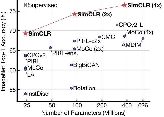
Figure 1: ImageNet Top-1 accuracy of linear classifiers trained on representations learned with different self-supervised methods (pretrained on ImageNet). Gray cross indicates supervised ResNet-50. Our method, SimCLR, is shown in bold.

图1:ImageNet Top-1精度线性分类者经过训练,掌握使用不同自监督方法(在ImageNet上预先训练)所学到的表示. Gray cross表示受监督的ResNet-50. 我们的方法,SimCLR,用粗体显示.

In this work, we introduce a simple framework for contrastive learning of visual representations, which we call SimCLR. Not only does SimCLR outperform previous work (Figure 1), but it is also simpler, requiring neither specialized architectures (Bachman et al., 2019; Hénaff et al., 2019) nor a memory bank (Wu et al., 2018; Tian et al., 2019; He et al., 2019; Misra & van der Maaten, 2019).

在这部作品中,我们引入了一个比较学习视觉表现的简单框架,我们称之为SimCLR. SimCLR不仅超越了以前的作品(图1),而且更为简单,既不需要专业建筑(Bachman等人,2019年;Hénaff等人,2019年),也不需要一个记忆库(Wu等人,2018年;Tian等人,2019年;He等人,2019年;Misra & van der Maaten,2019年).

In order to understand what enables good contrastive representation learning, we systematically study the major components of our framework and show that:

为了了解什么能促进良好的对比性代表性学习,我们系统地研究我们框架的主要组成部分,并表明:

• • Composition of multiple data augmentation operations is crucial in defining the contrastive prediction tasks that yield effective representations. In addition, unsupervised contrastive learning benefits from stronger data augmentation than supervised learning.
• • Introducing a learnable nonlinear transformation between the representation and the contrastive loss substantially improves the quality of the learned representations.
• • Representation learning with contrastive cross entropy loss benefits from normalized embeddings and an appropriately adjusted temperature parameter.
• • Contrastive learning benefits from larger batch sizes and longer training compared to its supervised counterpart. Like supervised learning, contrastive learning benefits from deeper and wider networks.

· 多重数据扩充业务的构成对于确定产生有效表示的对比预测任务至关重要。 此外,无监督的对比性学习比有监督的学习更能增加数据。
• 在代表性和对比性损失之间实行可学习的非线性转变,大大提高了学到的代表性的质量。
· 通过正规嵌入和适当调整的温度参数,利用对比性交叉演算损失来进行代表性学习。

• 与受监督的对口单位相比,批量较大、训练时间更长,学习效益相矛盾。 像受监督的学习一样,对比性的学习从更深入和更广泛的网络中获益。

We combine these findings to achieve a new state-of-the-art in self-supervised and semi-supervised learning on ImageNet ILSVRC-2012 (Russakovsky et al., 2015). Under the linear evaluation protocol, SimCLR achieves 76.5% top-1 accuracy, which is a 7% relative improvement over previous state-of-the-art (Hénaff et al., 2019). When fine-tuned with only 1% of the ImageNet labels, SimCLR achieves 85.8% top-5 accuracy, a relative improvement of 10% (Hénaff et al., 2019). When fine-tuned on other natural image classification datasets, SimCLR performs on par with or better than a strong supervised baseline (Kornblith et al., 2019) on 10 out of 12 datasets.

我们把这些调查结果结合起来,在ImageNet ILSVRC-2012上实现自监督和半监督学习的新先进水平(Russakovsky等人,2015年)。 根据线性评价协议,SimCLR达到了76.5%的顶级-1精度,比之前的先进水平(Hénaff等人,2019年)有7%的相对改进. 在仅用1%的ImageNet标签进行微调时,SimCLR实现了85.8%的上-5精度,相对改善10%(Hénaff等人,2019年). 在对其他自然图像分类数据集进行微调时,SimCLR在12个数据集中,有10个数据集的功能与强有力的监督基线相同或更好(Kornblith等人,2019年)。

2 Method

2 方法

2.1 The Contrastive Learning Framework

2.1 对比学习框架

Inspired by recent contrastive learning algorithms (see Section 7 for an overview), SimCLR learns representations by maximizing agreement between differently augmented views of the same data example via a contrastive loss in the latent space. As illustrated in Figure 2, this framework comprises the following four major components.

受最近对比性学习算法(参见第7节概述)的启发,SimCLR通过潜在空间的对比性损失,最大限度地实现对同一数据实例的不同增益观点之间的一致,从而学习表达式. 如图2所示,力求使该框架包括以下四个主要组成部分。

• • A stochastic data augmentation module that transforms any given data example randomly resulting in two correlated views of the same example, denoted $\tilde{\bm{x}}_{i}$ and $\tilde{\bm{x}}_{j}$, which we consider as a positive pair. In this work, we sequentially apply three simple augmentations: random cropping followed by resize back to the original size, random color distortions, and random Gaussian blur. As shown in Section 3, the combination of random crop and color distortion is crucial to achieve a good performance.
• • A neural network base encoder $f(\cdot)$ that extracts representation vectors from augmented data examples. Our framework allows various choices of the network architecture without any constraints. We opt for simplicity and adopt the commonly used ResNet (He et al., 2016) to obtain $\bm{h}_{i}=f(\tilde{\bm{x}}_{i})=\mathrm{ResNet}(\tilde{\bm{x}}_{i})$ where $\bm{h}_{i}\in\mathbb{R}^{d}$ is the output after the average pooling layer.
• • A small neural network projection head $g(\cdot)$ that maps representations to the space where contrastive loss is applied. We use a MLP with one hidden layer to obtain $\bm{z}_{i}=g(\bm{h}_{i})=W^{(2)}\sigma(W^{(1)}\bm{h}_{i})$ where $\sigma$ is a ReLU non-linearity. As shown in section 4, we find it beneficial to define the contrastive loss on $\bm{z}_{i}$’s rather than $\bm{h}_{i}$’s.
• • A contrastive loss function defined for a contrastive prediction task. Given a set $\{\tilde{\bm{x}}_{k}\}$ including a positive pair of examples $\tilde{\bm{x}}_{i}$ and $\tilde{\bm{x}}_{j}$, the contrastive prediction task aims to identify $\tilde{\bm{x}}_{j}$ in $\{\tilde{\bm{x}}_{k}\}_{k\neq i}$ for a given $\tilde{\bm{x}}_{i}$.

• 一个结构化的数据增强模块,将任何特定数据实例随机转换,导致同一实例的两个相关观点,表示XXMAT 你真是XX和$\tilde{\bm{x}}_{j}$,我们认为它们是正对。 在这部作品中,我们依次应用了三个简单的增强: 随机裁剪,然后调整大小回原大小, 随机色彩扭曲,和 随机高斯模糊. 如第3节所示,随机作物和颜色扭曲的组合对实现良好的性能至关重要。
• 神经网络 * 碱性编码器 *$f(\cdot)$从增加的数据示例中提取表示矢量。 我们的框架允许不受任何限制地选择网络架构。 我们选择简单化,采用常用的ResNet(He等人,2016年),以获得$\bm{h}_{i}=f(\tilde{\bm{x}}_{i})=\mathrm{ResNet}(\tilde{\bm{x}}_{i})$,其中$\bm{h}_{i}\in\mathbb{R}^{d}$是平均集合层后的输出.
• 一个小神经网络 * 投影头 * $g(\cdot)$,将表示图映射到应用对比性损失的空间。 我们用一个隐藏层的MLP来获得$\bm{z}_{i}=g(\bm{h}_{i})=W^{(2)}\sigma(W^{(1)}\bm{h}_{i})$,其中$\sigma$是ReLU的非线性. 如第4节所示,我们认为界定$\bm{z}_{i}$而不是$\bm{h}_{i}$的对比性损失是有益的。
• 为对比性预测任务确定的“连续损失函数”。 明天将举行为期一年的为期一年的为期一年的为期一年的为期一年的为期一年的为期一年的为期一年的为期一年的为期一年的为期一年的为期一年的为期一年的为期一年的为期一年的为期一年的为期一年的为期一年的为期一年的为期一年的为期一年的为期一年的为期一年的为期一年的为期一年的为期一年的为期一年的为期一年的为期一年的为期一年的为期一年的为期一年的为期一年的为期一年的为期一年的为期一年的为期一年的为期一年的为期一年的为期一年的为期一年的为期一年的为期一年的为期一年的为期一年的为期一年的为期一年的为期一年的为期一年的为期一年的为期一年的为期一年的为期一年的为期一年的为期一年的为期一年的为期为一年的为期一年的为期一年的为期一年的为期一年的为期为一年的为期一年的为期一年的为期一年的为期一年的为期一年的为期不超过一年的为期一年的为期一年的为期一年的为期一年的为期为一年的为期为一年的为期为一年的为期一年的为期一年的为期一年的为期为一年的为期一年的为期为一年的一年的

Figure 2: A simple framework for contrastive learning of visual representations. Two separate data augmentation operators are sampled from the same family of augmentations ($t\sim\mathcal{T}$ and $t^{\prime}\sim\mathcal{T}$) and applied to each data example to obtain two correlated views. A base encoder network $f(\cdot)$ and a projection head $g(\cdot)$ are trained to maximize agreement using a contrastive loss. After training is completed, we throw away the projection head $g(\cdot)$ and use encoder $f(\cdot)$ and representation $\bm{h}$ for downstream tasks.

图2:视觉表现对比性学习的简单框架. 对两个不同的数据增强操作员从同一个增强系统($t\sim\mathcal{T}$和$t^{\prime}\sim\mathcal{T}$)进行抽样,并应用于每个数据实例,以获取两个相关的观点。 一个基础编码器网络$f(\cdot)$和一个投影头$g(\cdot)$都经过了训练,以便利用对比性损失来达成最大的一致. 训练完成后,我们丢掉投影头$g(\cdot)$,用编码器$f(\cdot)$和代表器$\bm{h}$执行下游任务.

We randomly sample a minibatch of $N$ examples and define the contrastive prediction task on pairs of augmented examples derived from the minibatch, resulting in $2N$ data points. We do not sample negative examples explicitly. Instead, given a positive pair, similar to (Chen et al., 2017), we treat the other $2(N-1)$ augmented examples within a minibatch as negative examples. Let $\mathrm{sim}(\bm{u},\bm{v})=\bm{u}^{\top}\bm{v}/\lVert\bm{u}\rVert\lVert\bm{v}\rVert$ denote the dot product between $\ell_{2}$ normalized $\bm{u}$ and $\bm{v}$ (i.e. cosine similarity). Then the loss function for a positive pair of examples $(i,j)$ is defined as

31. 致致 致 备 的 致 的 致 的 致 的 致 的 致 收 的 致 的 致 的 致 的 致 的 致 的 致 的 致 的 致 的 致 的 致 的 的 致 的 的 致 的 的 致 的 的 的 迟 的 的 。 我们没有明确的抽样。 相反,给一个正对,类似于(Chen等人,2017年),我们把一个小批次中另一个$2(N-1)$的扩展例子当作负对例. 让$\mathrm{sim}(\bm{u},\bm{v})=\bm{u}^{\top}\bm{v}/\lVert\bm{u}\rVert\lVert\bm{v}\rVert$表示$\ell_{2}$正常化的$\bm{u}$和$\bm{v}$(即余弦相似性)之间的点产物. 然后,一个正对示例$(i,j)$的损失函数被定义为

$$\ell_{i,j}=-\log\frac{\exp(\mathrm{sim}(\bm{z}_{i},\bm{z}_{j})/\tau)}{\sum_{k=1}^{2N}\mathbbm{1}_{[k\neq i]}\exp(\mathrm{sim}(\bm{z}_{i},\bm{z}_{k})/\tau)}~, \tag{1}$$

where $\mathbbm{1}_{[k\neq i]}\in\{0,1\}$ is an indicator function evaluating to $1$ iff $k\neq i$ and $\tau$ denotes a temperature parameter. The final loss is computed across all positive pairs, both $(i,j)$ and $(j,i)$, in a mini-batch. This loss has been used in previous work (Sohn, 2016; Wu et al., 2018; Oord et al., 2018); for convenience, we term it NT-Xent (the normalized temperature-scaled cross entropy loss).

其中$\mathbbm{1}_{[k\neq i]}\in\{0,1\}$是一个指标函数,如果$k\neq i$和$\tau$表示温度参数,则该函数被评价为$1$. 最终损失是用小批量计算出的所有正对双,即$(i,j)$和$(j,i)$。 之前的作品(Sohn, 2016;Wu等人, 2018;Oord等人, 2018)中曾使用过这一损失;为方便起见,我们将其命名为NT-Xent(正常温度尺度的交叉肽损失).

Algorithm 1 summarizes the proposed method.

算法1总结了拟议方法.

input: batch size $N$, constant $\tau$, structure of $f$, $g$, $\mathcal{T}$.
for sampled minibatch $\{\bm{x}_{k}\}_{k=1}^{N}$ do
for all $k\in\{1,\ldots,N\}$ do
draw two augmentation functions $t\!\sim\!\mathcal{T}$, $t^{\prime}\!\sim\!\mathcal{T}$

the first augmentation

$\tilde{\bm{x}}_{2k-1}=t(\bm{x}_{k})$
$\bm{h}_{2k-1}=f(\tilde{\bm{x}}_{2k-1})$                               # representation
$\bm{z}_{2k-1}=g({\bm{h}}_{2k-1})$                                 # projection

the second augmentation

$\tilde{\bm{x}}_{2k}=t^{\prime}(\bm{x}_{k})$
$\bm{h}_{2k}=f(\tilde{\bm{x}}_{2k})$                                       # representation
$\bm{z}_{2k}=g({\bm{h}}_{2k})$                                         # projection
end for
for all $i\in\{1,\ldots,2N\}$ and $j\in\{1,\dots,2N\}$ do
$s_{i,j}=\bm{z}_{i}^{\top}\bm{z}_{j}/(\lVert\bm{z}_{i}\rVert\lVert\bm{z}_{j}\rVert)$         # pairwise similarity
end for
define $\ell(i,j)$ as  $\ell(i,j)\!=\!-\log\frac{\exp(s_{i,j}/\tau)}{\sum_{k=1}^{2N}\mathbbm{1}_{[k\neq i]}\exp(s_{i,k}/\tau)}$
$\mathcal{L}=\frac{1}{2N}\sum_{k=1}^{N}\left[\ell(2k\!-\!1,2k)+\ell(2k,2k\!-\!1)\right]$
update networks $f$ and $g$ to minimize $\mathcal{L}$
end for
return encoder network $f(\cdot)$, and throw away $g(\cdot)$

Algorithm 1 SimCLR’s main learning algorithm.

输入:批量大小$N$,常数$\tau$,结构为$f$,$g$,$\mathcal{T}$.
** 对于** 抽样的小批量$\{\bm{x}_{k}\}_{k=1}^{N}$** do**
** 所有国家**
绘制两个增强功能 $t\!\sim\!\mathcal{T}$, $t^{\prime}\!\sim\!\mathcal{T}$
第一次增强
第二十届
$\bm{h}_{2k-1}=f(\tilde{\bm{x}}_{2k-1})$ # 代表权
$\bm{z}_{2k-1}=g({\bm{h}}_{2k-1})$ # 预测
第二次增强
第二十二届
$\bm{h}_{2k}=f(\tilde{\bm{x}}_{2k})$ # 代表权
$\bm{z}_{2k}=g({\bm{h}}_{2k})$ # 预测
** 结束**
** 所有国家**
$s_{i,j}=\bm{z}_{i}^{\top}\bm{z}_{j}/(\lVert\bm{z}_{i}\rVert\lVert\bm{z}_{j}\rVert)$ # 双向相似性
** 结束**
定义$\ell(i,j)$ as$\ell(i,j)\!=\!-\log\frac{\exp(s_{i,j}/\tau)}{\sum_{k=1}^{2N}\mathbbm{1}_{[k\neq i]}\exp(s_{i,k}/\tau)}$
第二十届
更新网络 $f$和$g$,尽量减少$\mathcal{L}$
** 结束** ** 用于**
** 返回**编码器网络$f(\cdot)$,并丢弃$g(\cdot)$

** 算法 1** SimCLR的主要学习算法.

2.2 Training with Large Batch Size

2.2 用大批量训练

To keep it simple, we do not train the model with a memory bank (Wu et al., 2018; He et al., 2019). Instead, we vary the training batch size $N$ from 256 to 8192. A batch size of 8192 gives us 16382 negative examples per positive pair from both augmentation views. Training with large batch size may be unstable when using standard SGD/Momentum with linear learning rate scaling (Goyal et al., 2017). To stabilize the training, we use the LARS optimizer (You et al., 2017) for all batch sizes. We train our model with Cloud TPUs, using 32 to 128 cores depending on the batch size.[^2]

为了简单起见,我们不用记忆库来训练模型(Wu等人,2018年;He等人,2019年)。 相反,我们把训练批量的$N$从256个改为8192个。 批量大小为8192,从两个增益角度,每对正对给出16382个负例. 在使用具有线性学习速率尺度的标准SGD/Momentum(Goyal等人,2017年)时,大批量的训练可能不稳定。 为了稳定训练,我们使用LARS优化器(You et al., 2017)进行所有批量尺寸的训练. 我们用Cloud TPU训练我们的模型,根据批量大小使用32到128个核. [^2].

Global BN. Standard ResNets use batch normalization (Ioffe & Szegedy, 2015). In distributed training with data parallelism, the BN mean and variance are typically aggregated locally per device. In our contrastive learning, as positive pairs are computed in the same device, the model can exploit the local information leakage to improve prediction accuracy without improving representations. We address this issue by aggregating BN mean and variance over all devices during the training. Other approaches include shuffling data examples across devices (He et al., 2019), or replacing BN with layer norm (Hénaff et al., 2019).

** 全球BN**.标准ResNets使用批归一化(Ioffe & Szegedy,2015年)。 在具有数据并行性的分布式训练中,BN平均值和差异一般是每个设备在当地汇总的。 在我们的对比性学习中,由于正对在同一个设备中计算,该模型可以利用局部信息渗漏来提高预测的准确性而不改进表达. 我们通过汇总训练期间所有装置的BN平均值和差异来解决这一问题。 其他方法包括将数据实例分散到设备之间(He等人,2019年),或用层规范取代BN(Hénaff等人,2019年)。

2.3 Evaluation Protocol

2.3 评估协议

Here we lay out the protocol for our empirical studies, which aim to understand different design choices in our framework.

我们在此阐述了我们经验研究的程序,其目的是了解我们框架内的不同设计选择。

Dataset and Metrics. Most of our study for unsupervised pretraining (learning encoder network $f$ without labels) is done using the ImageNet ILSVRC-2012 dataset (Russakovsky et al., 2015). Some additional pretraining experiments on CIFAR-10 (Krizhevsky & Hinton, 2009) can be found in Appendix B.9. We also test the pretrained results on a wide range of datasets for transfer learning. To evaluate the learned representations, we follow the widely used linear evaluation protocol (Zhang et al., 2016; Oord et al., 2018; Bachman et al., 2019; Kolesnikov et al., 2019), where a linear classifier is trained on top of the frozen base network, and test accuracy is used as a proxy for representation quality. Beyond linear evaluation, we also compare against state-of-the-art on semi-supervised and transfer learning.

** 数据与计量。 ** 我们对无监督预训练(学习编码器网络$f$无标签)的研究大多使用ImageNet ILSVRC-2012数据集(Russakovsky等人,2015年)进行. 关于CIFAR-10(Krizhevsky & Hinton,2009年)的一些额外预训练实验可参见附录B.9. 我们还在各种用于转移学习的数据集上测试预先训练的结果。 为了评价学到的表达方式,我们遵循广泛使用的线性评价规程(张等,2016年;Oord等,2018年;Bachman等,2019年;Kolesnikov等,2019年),在冷冻基网顶部训练线性分类器,测试精度作为表示质量的代称. 除了线性评价外,我们还比较了半监督学习和转移学习的最新技术。

Default setting. Unless otherwise specified, for data augmentation we use random crop and resize (with random flip), color distortions, and Gaussian blur (for details, see Appendix A). We use ResNet-50 as the base encoder network, and a 2-layer MLP projection head to project the representation to a 128-dimensional latent space. As the loss, we use NT-Xent, optimized using LARS with learning rate of 4.8 ($=0.3\times\mathrm{BatchSize}/256$) and weight decay of $10^{-6}$. We train at batch size 4096 for 100 epochs.[^3] Furthermore, we use linear warmup for the first 10 epochs, and decay the learning rate with the cosine decay schedule without restarts (Loshchilov & Hutter, 2016).

** 过失设置。 ** 除非另有说明,在数据增强方面,我们使用随机裁剪和调整大小(带有随机翻转),色彩扭曲,以及高斯模糊(详情见附录A)。 我们使用ResNet-50作为基准编码器网络,和一个2层的MLP投影头来投影到一个128维的潜在空间. 作为损失,我们使用NT-Xent,优化使用LARS,学习率为4.8($=0.3\times\mathrm{BatchSize}/256$),重量衰减为$10^{-6}$. 我们以4096的批量规模训练100个世纪。[^3] 此外,我们对前10个纪元使用线性热身,不重启就用余弦衰减时间表来衰减学习率(Loshchilov & Hutter, 2016)。

3 Data Augmentation for Contrastive Representation Learning

3 对比表征学习中的数据增强

(a) Global and local views.

(a) 全球和地方观点。

(a) Original

(a) 原件

Data augmentation defines predictive tasks. While data augmentation has been widely used in both supervised and unsupervised representation learning (Krizhevsky et al., 2012; Hénaff et al., 2019; Bachman et al., 2019), it has not been considered as a systematic way to define the contrastive prediction task. Many existing approaches define contrastive prediction tasks by changing the architecture. For example, Hjelm et al. (2018); Bachman et al. (2019) achieve global-to-local view prediction via constraining the receptive field in the network architecture, whereas Oord et al. (2018); Hénaff et al. (2019) achieve neighboring view prediction via a fixed image splitting procedure and a context aggregation network. We show that this complexity can be avoided by performing simple random cropping (with resizing) of target images, which creates a family of predictive tasks subsuming the above mentioned two, as shown in Figure 3. This simple design choice conveniently decouples the predictive task from other components such as the neural network architecture. Broader contrastive prediction tasks can be defined by extending the family of augmentations and composing them stochastically.

** 数据增强定义了预测性任务。 ** 虽然数据扩增被广泛用于监督和非监督的表达学习(Krizhevsky等人,2012年;Hénaff等人,2019年;Bachman等人,2019年),但并未被视为定义对比性预测任务的系统方法. 许多现有方法通过改变架构来定义对比性预测任务. 例如,Hjelm等人(2018年);Bachman等人(2019年)通过限制网络架构中的可接受性领域实现全局到局部视图预测,而Oord等人(2018年);Hénaff等人(2019年)通过固定的图像分割程序和上下文聚合网络实现相邻视图预测. 我们表明,通过对目标图像进行简单的随机收割(再生),可以避免这种复杂性,这将形成一个预测性任务家族,将上述两个任务归并,如图3所示。 这种简单的设计选择方便地将预测性任务与神经网络架构等其他组件脱钩. 比较广泛的对比性预测任务可以通过扩展增殖的家族来定义,并按部就班地加以组合.

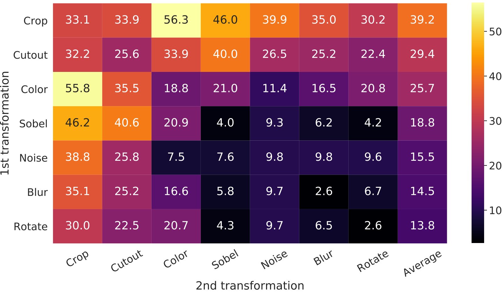
Figure 5: Linear evaluation (ImageNet top-1 accuracy) under individual or composition of data augmentations, applied only to one branch. For all columns but the last, diagonal entries correspond to single transformation, and off-diagonals correspond to composition of two transformations (applied sequentially). The last column reflects the average over the row.

图5:数据扩增的单个或构成下的线性评价(ImageNet顶级-1精度),仅适用于一个分支. 对于除最后一个外的所有列,对角条目对应单一变换,对角部分对应两个变换的构成(按顺序应用). 最后一栏反映了该行的平均数。

3.1 Composition of data augmentation operations is crucial for learning good representations

3.1 数据增强操作的组合对学好表征至关重要

To systematically study the impact of data augmentation, we consider several common augmentations here. One type of augmentation involves spatial/geometric transformation of data, such as cropping and resizing (with horizontal flipping), rotation (Gidaris et al., 2018) and cutout (DeVries & Taylor, 2017). The other type of augmentation involves appearance transformation, such as color distortion (including color dropping, brightness, contrast, saturation, hue) (Howard, 2013; Szegedy et al., 2015), Gaussian blur, and Sobel filtering. Figure 4 visualizes the augmentations that we study in this work.

为了系统地研究数据扩充的影响,我们在此考虑若干共同的扩充。 一种增强方式涉及数据的空间/几何转换,如裁剪和再大小(带有水平翻转),旋转(Gidaris等人,2018年)和剪切(DeVries & Taylor,2017年). 另一种增强方式涉及外观变换,如色彩扭曲(包括颜色下降,亮度,对比度,饱和度,hue)(Howard,2013年;Szegedy等人,2015年),高斯模糊,以及索贝尔过滤. 图4显示了我们在这项工作中研究的增强。

To understand the effects of individual data augmentations and the importance of augmentation composition, we investigate the performance of our framework when applying augmentations individually or in pairs. Since ImageNet images are of different sizes, we always apply crop and resize images (Krizhevsky et al., 2012; Szegedy et al., 2015), which makes it difficult to study other augmentations in the absence of cropping. To eliminate this confound, we consider an asymmetric data transformation setting for this ablation. Specifically, we always first randomly crop images and resize them to the same resolution, and we then apply the targeted transformation(s) only to one branch of the framework in Figure 2, while leaving the other branch as the identity (i.e. $t(\bm{x}_{i})=\bm{x}_{i}$). Note that this asymmetric data augmentation hurts the performance. Nonetheless, this setup should not substantively change the impact of individual data augmentations or their compositions.

为了了解单个数据扩增的影响和扩增构成的重要性,我们在单独或成对地应用扩增时调查我们框架的表现。 由于ImageNet的图像大小不同,我们总是应用裁剪和缩放图像(Krizhevsky等人,2012年;Szegedy等人,2015年),这使得在没有裁剪的情况下难以研究其他增强. 为消除这种混乱,我们考虑为这种萎缩设置不对称的数据转换。 具体来说,我们总是先随机裁剪图像,然后将其大小调整到同一个分辨率,然后对图2中框架的一个分支(即$t(\bm{x}_{i})=\bm{x}_{i}$)应用目标变换**. 注意这种不对称的数据增强会损害性能. 然而,这种设置不应实质性地改变个别数据扩充的影响或其组成。

Figure 5 shows linear evaluation results under individual and composition of transformations. We observe that no single transformation suffices to learn good representations, even though the model can almost perfectly identify the positive pairs in the contrastive task. When composing augmentations, the contrastive prediction task becomes harder, but the quality of representation improves dramatically. Appendix B.2 provides a further study on composing broader set of augmentations.

图5显示个别和转型构成下的线性评价结果。 我们观察到,没有一个单一的转变足以学习好的表达式,尽管模型几乎可以完美地识别对比性任务中的正对. 在编组增强时,对比性的预测任务变得更加困难,但表述质量大为提高. 附录B.2对构成更广泛的增强部分作了进一步研究。

One composition of augmentations stands out: random cropping and random color distortion. We conjecture that one serious issue when using only random cropping as data augmentation is that most patches from an image share a similar color distribution. Figure 6 shows that color histograms alone suffice to distinguish images. Neural nets may exploit this shortcut to solve the predictive task. Therefore, it is critical to compose cropping with color distortion in order to learn generalizable features.

扩增的一个成分突出:随机裁剪和随机色彩扭曲. 我们猜想,在仅仅使用随机裁剪作为数据增强时,一个严重的问题是,来自图像的大部分补丁都具有类似的颜色分布。 图6显示,仅彩色直方图就足以区分图像。 神经网可能利用这个捷径来解决预测性任务. 因此,至关重要的是用色彩扭曲来编织作物,以便学习一般特征。

(a) Without color distortion.

(a) 不扭曲颜色。

3.2 Contrastive learning needs stronger data augmentation than supervised learning

3.2 对比学习需要比监督学习更强的数据增强

	Color distortion strength
Methods	1/8	1/4	1/2	1	1 (+Blur)	AutoAug
SimCLR	59.6	61.0	62.6	63.2	64.5	61.1
Supervised	77.0	76.7	76.5	75.7	75.4	77.1

Table 1: Top-1 accuracy of unsupervised ResNet-50 using linear evaluation and supervised ResNet-50[^5], under varied color distortion strength (see Appendix A) and other data transformations. Strength 1 (+Blur) is our default data augmentation policy.

	颜色扭曲强度
方法	1/8	1/4	1/2	1	1 (+Blur) (韩语)	自动Aug
SimCLR 数据	59.6	61.0	62.6	63.2	64.5	61.1
监督	77.0	76.7	76.5	75.7	75.4	77.1

表1:无监督的ResNet-50使用线性评价和受监督的ResNet-50[^5],在不同的颜色扭曲强度下(见附录A)和其他数据转换的顶-1精度. 强1(+Blur)是我们的默认数据增强政策.

To further demonstrate the importance of the color augmentation, we adjust the strength of color augmentation as shown in Table 1. Stronger color augmentation substantially improves the linear evaluation of the learned unsupervised models. In this context, AutoAugment (Cubuk et al., 2019), a sophisticated augmentation policy found using supervised learning, does not work better than simple cropping + (stronger) color distortion. When training supervised models with the same set of augmentations, we observe that stronger color augmentation does not improve or even hurts their performance. Thus, our experiments show that unsupervised contrastive learning benefits from stronger (color) data augmentation than supervised learning. Although previous work has reported that data augmentation is useful for self-supervised learning (Doersch et al., 2015; Bachman et al., 2019; Hénaff et al., 2019; Asano et al., 2019), we show that data augmentation that does not yield accuracy benefits for supervised learning can still help considerably with contrastive learning.

为进一步展示增色的重要性,我们调整了表1所示的增色强度. 更强的色彩增强大大改进了对所学的无监督模型的线性评价. 在这方面,AutoAugment(Cubuk等人,2019年)是一种复杂的增强政策,它采用监督学习的方式,但并不比简单的裁剪+(更强烈的)色彩扭曲更好。 当训练有监督的模型 具有相同的增强, 我们发现, 更强的色彩增强 没有改善甚至损害 它们的性能。 因此,我们的实验表明,无监督的对比性学习比有监督的学习更能增强数据。 虽然先前的工作报告称数据扩增对自监督的学习很有用(Doersch等人,2015年;Bachman等人,2019年;Hénaff等人,2019年;Asano等人,2019年),但我们显示,数据扩增不能为监督的学习带来准确性好处,仍然可以极大地帮助对比性学习.

4 Architectures for Encoder and Head

4 编码器与投影头的架构

4.1 Unsupervised contrastive learning benefits (more) from bigger models

4.1 无监督对比学习从更大模型中受益（更多）

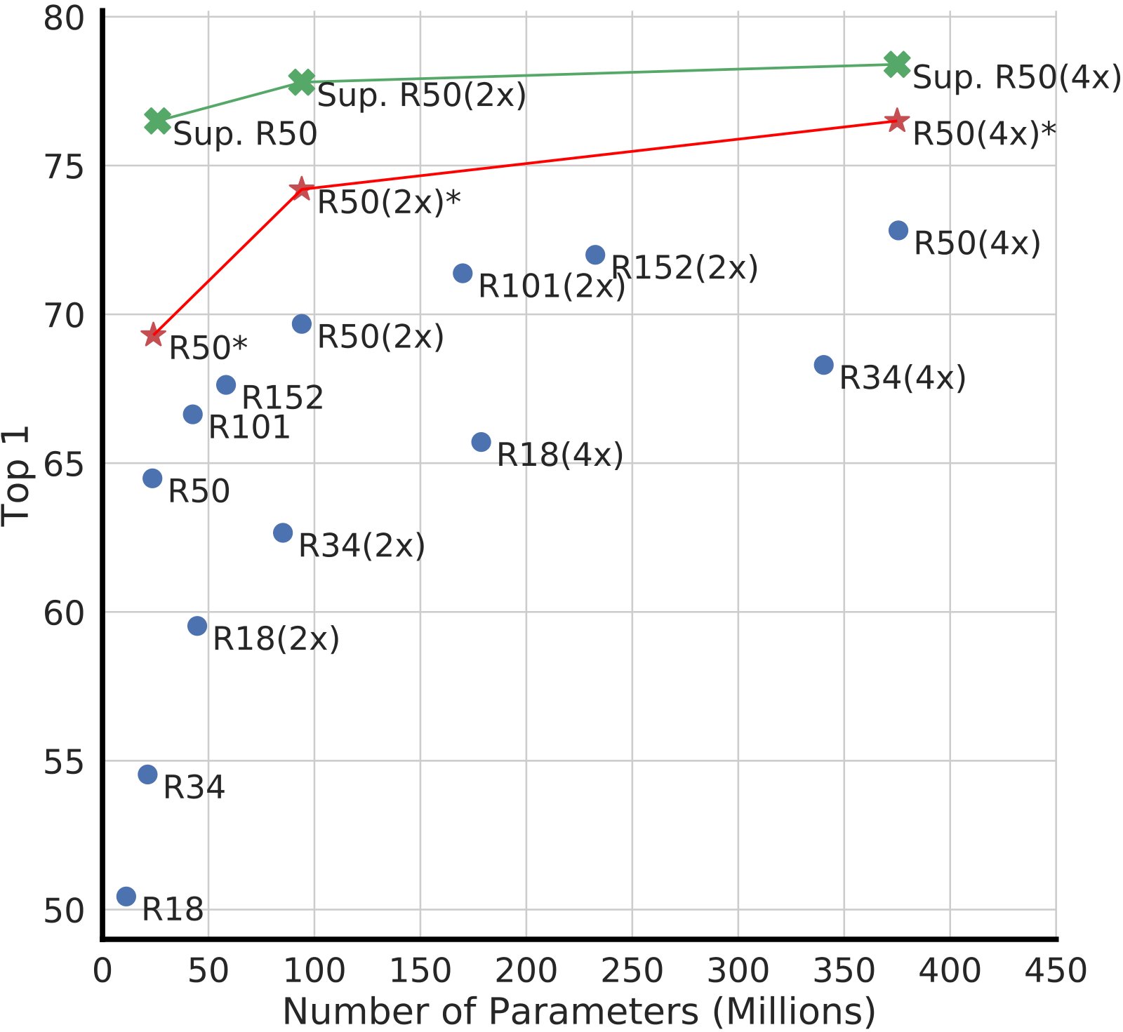
Figure 7: Linear evaluation of models with varied depth and width. Models in blue dots are ours trained for 100 epochs, models in red stars are ours trained for 1000 epochs, and models in green crosses are supervised ResNets trained for 90 epochs[^7] (He et al., 2016).

图7 对深度和宽度各不相同的模型进行线性评价。 蓝点模型是我们为100个纪元而训练的,红星模型是我们为1000个纪元而训练的,绿色十字模型被监督ResNets为90个纪元而训练的^7.

Figure 7 shows, perhaps unsurprisingly, that increasing depth and width both improve performance. While similar findings hold for supervised learning (He et al., 2016), we find the gap between supervised models and linear classifiers trained on unsupervised models shrinks as the model size increases, suggesting that unsupervised learning benefits more from bigger models than its supervised counterpart.

图7显示,也许不足为奇的是,深度和宽度的提高都改善了业绩。 虽然类似的发现对有监督的学习很重要(He等人,2016年),但我们发现,在无监督模型方面受过训练的有监督模型和线性分类者之间的差距随着模型大小的增加而缩小,这表明,无监督的学习比其有监督的对应者 更能从更大的模型中获益。

Name	Negative loss function	Gradient w.r.t. $\bm{u}$
NT-Xent	$\bm{u}^{T}\bm{v}^{+}/\tau-\log\sum_{\bm{v}\in\{\bm{v}^{+},\bm{v}^{-}\}}\exp(\bm{u}^{T}\bm{v}/\tau)$	$(1-\frac{\exp(\bm{u}^{T}\bm{v}^{+}/\tau)}{Z(\bm{u})})/\tau\bm{v}^{+}-\sum_{\bm{v}^{-}}\frac{\exp(\bm{u}^{T}\bm{v}^{-}/\tau)}{Z(\bm{u})}/\tau\bm{v}^{-}$
NT-Logistic	$\log\sigma(\bm{u}^{T}\bm{v}^{+}/\tau)+\log\sigma(-\bm{u}^{T}\bm{v}^{-}/\tau)$	$(\sigma(-\bm{u}^{T}\bm{v}^{+}/\tau))/\tau\bm{v}^{+}-\sigma(\bm{u}^{T}\bm{v}^{-}/\tau)/\tau\bm{v}^{-}$
Margin Triplet	$-\max(\bm{u}^{T}\bm{v}^{-}-\bm{u}^{T}\bm{v}^{+}+m,0)$	$\bm{v}^{+}-\bm{v}^{-}\text{ if }\bm{u}^{T}\bm{v}^{+}-\bm{u}^{T}\bm{v}^{-}<m\text{ else }\bm{0}$

Table 2: Negative loss functions and their gradients. All input vectors, i.e. $\bm{u},\bm{v}^{+},\bm{v}^{-}$, are $\ell_{2}$ normalized. NT-Xent is an abbreviation for “Normalized Temperature-scaled Cross Entropy”. Different loss functions impose different weightings of positive and negative examples.

我们可以用这把刀	负损失函数	Gradient w.r.t. $\bm{u}$
NT - X 类型	第二十届	第二十届
NT- 逻辑	第二十届	第二十届
边距三进制	$-\max(\bm{u}^{T}\bm{v}^{-}-\bm{u}^{T}\bm{v}^{+}+m,0)$	第二十届

表2:负损失函数及其梯度。 所有输入向量,即$\bm{u},\bm{v}^{+},\bm{v}^{-}$,均实现$\ell_{2}$正常化. NT-Xent是“Normalized Went-scaled Cross Entropy”的缩写。 不同的损失函数对正负例子规定了不同的权重.

4.2 A nonlinear projection head improves the representation quality of the layer before it

4.2 非线性投影头能提升其之前一层的表征质量

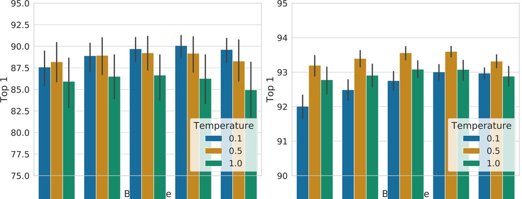
Figure 8: Linear evaluation of representations with different projection heads $g(\cdot)$ and various dimensions of $\bm{z}=g(\bm{h})$. The representation $\bm{h}$ (before projection) is 2048-dimensional here.

图8:对不同投影头$g(\cdot)$和$\bm{z}=g(\bm{h})$不同维度的表示进行线性评价. 表示式$\bm{h}$(在投影前)在此为2048维.

We then study the importance of including a projection head, i.e. $g(\bm{h})$. Figure 8 shows linear evaluation results using three different architecture for the head: (1) identity mapping; (2) linear projection, as used by several previous approaches (Wu et al., 2018); and (3) the default nonlinear projection with one additional hidden layer (and ReLU activation), similar to Bachman et al. (2019). We observe that a nonlinear projection is better than a linear projection (+3%), and much better than no projection (>10%). When a projection head is used, similar results are observed regardless of output dimension. Furthermore, even when nonlinear projection is used, the layer before the projection head, $\bm{h}$, is still much better (>10%) than the layer after, $\bm{z}=g(\bm{h})$, which shows that the hidden layer before the projection head is a better representation than the layer after.

然后,我们研究列入一个投影头,即$g(\bm{h})$的重要性。 图8采用三种不同架构对头进行线性评价的结果: (1)身份映射; (2)线性投影,如之前的几种方法(Wu等人,2018年); (3)默认的非线性投影,再增加一个隐藏层(和ReLU激活),类似于Bachman等人(2019年). 我们认为,非线性预测比线性预测(+3%)好,比无线性预测(>10%)好得多。 在使用投影头时,无论输出大小,都观察到类似的结果. 此外,即使在使用非线性投影时,投影头前的层,$\bm{h}$,仍然比之后的层,$\bm{z}=g(\bm{h})$,要好得多(>10%),这表明,投影头前的隐藏层,比之后的层要好得多.

We conjecture that the importance of using the representation before the nonlinear projection is due to loss of information induced by the contrastive loss. In particular, $\bm{z}=g(\bm{h})$ is trained to be invariant to data transformation. Thus, $g$ can remove information that may be useful for the downstream task, such as the color or orientation of objects. By leveraging the nonlinear transformation $g(\cdot)$, more information can be formed and maintained in $\bm{h}$. To verify this hypothesis, we conduct experiments that use either $\bm{h}$ or $g(\bm{h})$ to learn to predict the transformation applied during the pretraining. Here we set $g(h)=W^{(2)}\sigma(W^{(1)}h)$, with the same input and output dimensionality (i.e. 2048). Table 3 shows $\bm{h}$ contains much more information about the transformation applied, while $g(\bm{h})$ loses information. Further analysis can be found in Appendix B.4.

我们推测,在非线性预测之前使用表述的重要性,是由于相对损失导致的信息丢失。 特别是,$\bm{z}=g(\bm{h})$被训练成对数据转换不具有变化性. 因此,$g$可以删除可能对下游任务有用的信息,如物体的颜色或方向. 通过利用非线性转换$g(\cdot)$,可以在$\bm{h}$中形成和维护更多信息. 为了验证这个假说,我们进行实验,使用$\bm{h}$或$g(\bm{h})$来学习预测在预训练期间应用的转化. 在这里,我们设定了$g(h)=W^{(2)}\sigma(W^{(1)}h)$,输入和输出维度相同(即2048)。 表3显示$\bm{h}$包含更多关于所应用的转换的信息,而$g(\bm{h})$丢失信息. 进一步的分析见附录B.4。

What to predict?	Random guess	Representation
$\bm{h}$	$g(\bm{h})$
Color vs grayscale	80	99.3	97.4
Rotation	25	67.6	25.6
Orig. vs corrupted	50	99.5	59.6
Orig. vs Sobel filtered	50	96.6	56.3

Table 3: Accuracy of training additional MLPs on different representations to predict the transformation applied. Other than crop and color augmentation, we additionally and independently add rotation (one of $\{0\degree,90\degree,180\degree,270\degree\}$), Gaussian noise, and Sobel filtering transformation during the pretraining for the last three rows. Both $\bm{h}$ and $g(\bm{h})$ are of the same dimensionality, i.e. 2048.

预测什么?	随机猜测	代表权
$\bm{h}$	$g(\bm{h})$
颜色对灰度	80	99.3	97.4
旋转	25	67.6	25.6
奥瑞格 vs 腐败	50	99.5	59.6
奥瑞格 vs Sobel 过滤	50	96.6	56.3

表3:为预测所应用的转变,对不同的表述方式进行额外中期规划训练的准确性。 除了作物和色彩增强,我们额外和独立地增加了旋转($\{0\degree,90\degree,180\degree,270\degree\}$之一),高斯噪音,以及索贝尔在前三行预训练期间的过滤转换. $\bm{h}$和$g(\bm{h})$都具有相同的维度,即2048.

5 Loss Functions and Batch Size

5 损失函数与批量大小

5.1 Normalized cross entropy loss with adjustable temperature works better than alternatives

5.1 带可调温度的归一化交叉熵损失优于其他选择

We compare the NT-Xent loss against other commonly used contrastive loss functions, such as logistic loss (Mikolov et al., 2013), and margin loss (Schroff et al., 2015). Table 2 shows the objective function as well as the gradient to the input of the loss function. Looking at the gradient, we observe 1) $\ell_{2}$ normalization (i.e. cosine similarity) along with temperature effectively weights different examples, and an appropriate temperature can help the model learn from hard negatives; and 2) unlike cross-entropy, other objective functions do not weigh the negatives by their relative hardness. As a result, one must apply semi-hard negative mining (Schroff et al., 2015) for these loss functions: instead of computing the gradient over all loss terms, one can compute the gradient using semi-hard negative terms (i.e., those that are within the loss margin and closest in distance, but farther than positive examples).

我们比较NT-Xent损失与其他常用的对比性损失功能,如后勤损失(Mikolov等人,2013年)和保证金损失(Schroff等人,2015年)。 表2显示损失函数输入的目标函数和梯度。 从梯度看,我们观察到1)$\ell_{2}$正常化(即同位素相似性)与温度有效加权不同的例子,适当的温度可以帮助模型从硬负数中学习;2) 与跨正负值不同的是,其他客观函数不会用相对硬度来权衡负值. 因此,对这些损失函数必须采用半硬性负采矿法(Schroff等人,2015年):人们不能够计算所有损失条款的梯度,而可以使用半硬性负词(即那些在损失幅度内且距离最近,但比正例更远)计算梯度。

To make the comparisons fair, we use the same $\ell_{2}$ normalization for all loss functions, and we tune the hyperparameters, and report their best results.[^8] Table 4 shows that, while (semi-hard) negative mining helps, the best result is still much worse than our default NT-Xent loss.

为了进行公平的比较,我们对所有损失函数使用相同的$\ell_{2}$正常化,调整超参数,并报告其最佳结果。 表4显示,虽然(半硬的)负面开采有帮助,但最佳结果仍然比我们默认的NT-Xent损失要糟糕得多。

We next test the importance of the $\ell_{2}$ normalization (i.e. cosine similarity vs dot product) and temperature $\tau$ in our default NT-Xent loss. Table 5 shows that without normalization and proper temperature scaling, performance is significantly worse. Without $\ell_{2}$ normalization, the contrastive task accuracy is higher, but the resulting representation is worse under linear evaluation.

我们接下来检验$\ell_{2}$正常化(即余弦相似度与点产品)和温度$\tau$在我们默认NT-Xent损失中的重要性. 表5显示,如果没有正常化和适当的温度缩放,性能就会大为恶化。 没有$\ell_{2}$正常化,对比性任务精确度更高,但在线性评价下,由此产生的表述更糟糕.

Margin	NT-Logi.	Margin (sh)	NT-Logi.(sh)	NT-Xent
50.9	51.6	57.5	57.9	63.9

Table 4: Linear evaluation (top-1) for models trained with different loss functions. “sh” means using semi-hard negative mining.

边距	(原始内容存档于2018-09-13). NT-Logi.	边距 (sh)	NT-Logi. (sh) (英语).	NT - X 类型
50.9	51.6	57.5	57.9	63.9

表4:经过不同损失功能训练的模型的线性评价(上-1). “sh”是指使用半硬性负式采矿。

$\ell_{2}$ norm?	$\tau$	Entropy	Contrastive acc.	Top 1
Yes	0.05	1.0	90.5	59.7
0.1	4.5	87.8	64.4
0.5	8.2	68.2	60.7
1	8.3	59.1	58.0
No	10	0.5	91.7	57.2
100	0.5	92.1	57.0

Table 5: Linear evaluation for models trained with different choices of $\ell_{2}$ norm and temperature $\tau$ for NT-Xent loss. The contrastive distribution is over 4096 examples.

$\ell_{2}$规范?	$\tau$	环形	(原始内容存档于2018-09-26). Extrastic acc.	顶级 1
对	0.05	1.0	90.5	59.7
0.1	4.5	87.8	64.4
0.5	8.2	68.2	60.7
1	8.3	59.1	58.0
没有	10	0.5	91.7	57.2
100	0.5	92.1	57.0

表5:对经过训练 60. $\ell_{2}$规范不同选择的模型进行线性评价,对NT-Xent损失进行温度 $\tau$。 对比分布超过4096例.

5.2 Contrastive learning benefits (more) from larger batch sizes and longer training

5.2 对比学习从更大 batch 与更长训练中受益（更多）

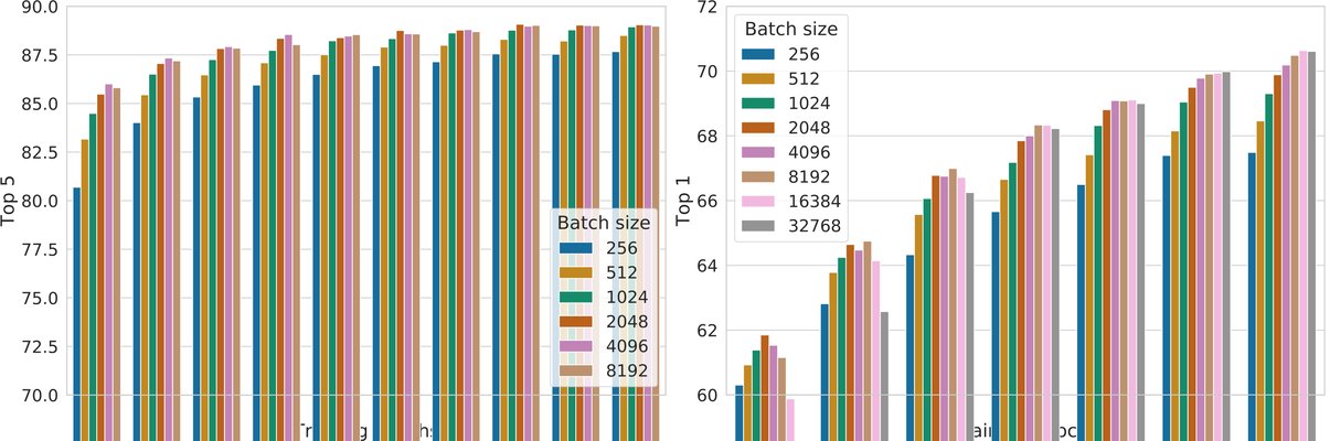
Figure 9: Linear evaluation models (ResNet-50) trained with different batch size and epochs. Each bar is a single run from scratch.[^10]

图9:线性评价模型(ResNet-50)经过不同批量大小和时代的训练。 每个栏杆都是从零开始的单跑 [^10].

Figure 9 shows the impact of batch size when models are trained for different numbers of epochs. We find that, when the number of training epochs is small (e.g. 100 epochs), larger batch sizes have a significant advantage over the smaller ones. With more training steps/epochs, the gaps between different batch sizes decrease or disappear, provided the batches are randomly resampled. In contrast to supervised learning (Goyal et al., 2017), in contrastive learning, larger batch sizes provide more negative examples, facilitating convergence (i.e. taking fewer epochs and steps for a given accuracy). Training longer also provides more negative examples, improving the results. In Appendix B.1, results with even longer training steps are provided.

图9显示模型为不同数目的纪元训练时批量大小的影响. 我们发现,当训练时代的数量很少(例如100个时代)时,较大的批量规模比较小的有显著优势. 随着训练步骤/时间的增多,不同批次尺寸之间的差距缩小或消失,只要批次被随机重印. 与监督学习形成对比(Goyal等人,2017年),在对比学习中,较大的批量大小提供了更多的负面例子,促进了趋同(即为给定准确性采取较少的时代和步骤). 训练时间更长也提供了更多的负面例子,改善了结果。 附录B.1提供了训练步骤更长的成果。

Method	Architecture	Param (M)	Top 1	Top 5
Methods using ResNet-50:
Local Agg.	ResNet-50	24	60.2	-
MoCo	ResNet-50	24	60.6	-
PIRL	ResNet-50	24	63.6	-
CPC v2	ResNet-50	24	63.8	85.3
SimCLR (ours)	ResNet-50	24	69.3	89.0
Methods using other architectures:
Rotation	RevNet-50 ($4\times$)	86	55.4	-
BigBiGAN	RevNet-50 ($4\times$)	86	61.3	81.9
AMDIM	Custom-ResNet	626	68.1	-
CMC	ResNet-50 ($2\times$)	188	68.4	88.2
MoCo	ResNet-50 ($4\times$)	375	68.6	-
CPC v2	ResNet-161 ($*$)	305	71.5	90.1
SimCLR (ours)	ResNet-50 ($2\times$)	94	74.2	92.0
SimCLR (ours)	ResNet-50 ($4\times$)	375	76.5	93.2

Table 6: ImageNet accuracies of linear classifiers trained on representations learned with different self-supervised methods.

方法	建筑	参数( M)	顶级 1	前5类
shin-50方法:
当地人Agg.	有助于促进家庭发展	24	60.2	-
如何能够让MoCo	ResNet-50 网络	24	60.6	-
总统	ResNet-50 网络	24	63.6	-
产品总分类v2	是否可以使用网络50	24	63.8	85.3
SimCLR (我们)	ResNet-50 网络	24	页:1	页:1
* 使用其他架构的方法:*
旋转	RevNet-50($4\times$) (中文( 增编) ).	86	55.4	-
大边疆	Rev提供资料 你在说什么?	86	61.3	81.9
阿曼	自定义网络	626	68.1	-
社区监测中心	ResNet-50($2\times$ ) (中文(简体) ).	188	68.4	88.2
你为什么要这么做?	ResNet-50($4\times$ ) (中文(简体) ).	375	68.6	-
产品总分类v2	ResNet-161 ($*$)	305	71.5	90.1
SimCLR (我们)	ResNet-50($2\times$ ) (中文(简体) ).	94	74.2	92.0
SimCLR( 我们)	ResNet-50($4\times$ ) (中文(简体) ).	375	** 第76.5段**	93.2 经常预算:

表6:ImageNet精准的线性分类人员接受过不同自监督方法所学习的表达法训练.

Method	Architecture	Label fraction
1%	10%
Top 5
Supervised baseline	ResNet-50	48.4	80.4
Methods using other label-propagation:
Pseudo-label	ResNet-50	51.6	82.4
VAT+Entropy Min.	ResNet-50	47.0	83.4
UDA (w. RandAug)	ResNet-50	-	88.5
FixMatch (w. RandAug)	ResNet-50	-	89.1
S4L (Rot+VAT+En. M.)	ResNet-50 (4$\times$)	-	91.2
Methods using representation learning only:
InstDisc	ResNet-50	39.2	77.4
BigBiGAN	RevNet-50 ($4\times$)	55.2	78.8
PIRL	ResNet-50	57.2	83.8
CPC v2	ResNet-161($*$)	77.9	91.2
SimCLR (ours)	ResNet-50	75.5	87.8
SimCLR (ours)	ResNet-50 ($2\times$)	83.0	91.2
SimCLR (ours)	ResNet-50 ($4\times$)	85.8	92.6

Table 7: ImageNet accuracy of models trained with few labels.

方法	建筑	标签分数
1%	10%
前5类
监督基线	ResNet-50 网络	48.4	80.4
* 使用其他标签传播的方法:*
修道士标签	ResNet-50 网络	51.6	82.4
增值税+进取税.	ResNet-50 网络	47.0	83.4
U的设想( W. RandAug)	ResNet-50 (韩语)	-	88.5
FixMatch (w. RandAug) (英语).	ResNet-50 网络	-	89.1
S Bauers (Rot+VAT+En. M.) (英语:	ResNet-50 (4$\times$) (中文(简体) ).	-	91.2
* 仅使用代表学习的方法:*
硬盘	ResNet-50 网络	39.2	77.4
大边疆	RevNet-50($4\times$) (中文(简体) ).	55.2	78.8
总统	ResNet-50 网络	57.2	83.8
产品总分类v2	ResNet-161($*$)	77.9	91.2
SimCLR (我们)	ResNet-50 网络	75.5	87.8
SimCLR (我们)	ResNet-50($2\times$ ) (中文(简体) ).	83.0	91.2
SimCLR (我们)	ResNet-50($4\times$ ) (中文(简体) ).	**的一般性说明。	92.6 国家

表7:经过训练且标签很少的模型的ImageNet精度.

	Food	CIFAR10	CIFAR100	Birdsnap	SUN397	Cars	Aircraft	VOC2007	DTD	Pets	Caltech-101	Flowers
Linear evaluation:
SimCLR (ours)	76.9	95.3	80.2	48.4	65.9	60.0	61.2	84.2	78.9	89.2	93.9	95.0
Supervised	75.2	95.7	81.2	56.4	64.9	68.8	63.8	83.8	78.7	92.3	94.1	94.2
Fine-tuned:
SimCLR (ours)	89.4	98.6	89.0	78.2	68.1	92.1	87.0	86.6	77.8	92.1	94.1	97.6
Supervised	88.7	98.3	88.7	77.8	67.0	91.4	88.0	86.5	78.8	93.2	94.2	98.0
Random init	88.3	96.0	81.9	77.0	53.7	91.3	84.8	69.4	64.1	82.7	72.5	92.5

Table 8: Comparison of transfer learning performance of our self-supervised approach with supervised baselines across 12 natural image classification datasets, for ResNet-50 $(4\times)$ models pretrained on ImageNet. Results not significantly worse than the best ($p>0.05$, permutation test) are shown in bold. See Appendix B.8 for experimental details and results with standard ResNet-50.

	粮食	第10条	中非共和国100	鸟巢	第397号	汽车	飞机	VOC 2007 (英语).	发展	宠物	Cal霞科技101	鲜花
* 参考评价:*
SimCLR (我们)	页:1	页:1	80.2	48.4	** 第65.9段 **	60.0	61.2	页:1	** ** 78.9 **	89.2	页:1	页:1
监督	75.2	页:1	** 81.2** 国家	页:1	64.9	** 68.8** (单位:千美元)	页:1	83.8	页:1	页:1	94.1 (单位:千美元)	94.2
*好调: *
SimCLR (我们)	页:1	** 98.6 **	页:1	页:1	** 68.1 **	92.1 国家	页:1	页:1	** 77.8** (单位:千美元)	92.1	94.1 (单位:千美元)	97.6
监督	88.7	98.3	88.7 (单位:千美元)	** 77.8** (单位:千美元)	67.0	91.4	** ** 88.0** (单位:千美元)	86.5	页:1	93.2 经常预算:	** 94.2 **	**98.0آ
随机输入	88.3	96.0	81.9	页:1	53.7	91.3	84.8	69.4	64.1	82.7	72.5	92.5

表8:对ResNet-50 $(4\times)$模型在ImageNet上预先训练的自监督方法的转让学习绩效与12个自然图像分类数据集的受监督基线的比较。 以粗体显示的结果并不比最好的结果($p>0.05$,穿透测试)差。 关于试验细节和结果,见附录B.8,以及标准ResNet-50。

6 Comparison with State-of-the-art

6 与当时最佳方法的比较

In this subsection, similar to Kolesnikov et al. (2019); He et al. (2019), we use ResNet-50 in 3 different hidden layer widths (width multipliers of $1\times$, $2\times$, and $4\times$). For better convergence, our models here are trained for 1000 epochs.

在本小节中,与Kolesnikov等人(2019年);He等人(2019年)相似,我们在3个不同的隐藏层宽度($1\times$,$2\times$和$4\times$的width乘数)中使用ResNet-50. 为了更好的趋同,我们这里的模型被训练了1000个世纪。

Linear evaluation. Table 6 compares our results with previous approaches (Zhuang et al., 2019; He et al., 2019; Misra & van der Maaten, 2019; Hénaff et al., 2019; Kolesnikov et al., 2019; Donahue & Simonyan, 2019; Bachman et al., 2019; Tian et al., 2019) in the linear evaluation setting (see Appendix B.6). Table 1 shows more numerical comparisons among different methods. We are able to use standard networks to obtain substantially better results compared to previous methods that require specifically designed architectures. The best result obtained with our ResNet-50 ($4\times$) can match the supervised pretrained ResNet-50.

** 评价。 ** 表6 将我们的结果与以往的方法(Zhuang等人,2019年;He等人,2019年;Misra & van der Maaten,2019年;Hénaff等人,2019年;Kolesnikov等人,2019年;Donahue & Simonyan,2019年;Bachman等人,2019年;Tian等人,2019年)在线性评估中进行比较(见附录B.6)。 表1显示不同方法之间的数字比较较多。 与以前需要专门设计的建筑相比,我们能够使用标准网络来取得更好的结果。 通过我们的ResNet-50($4\times$)获得的最佳结果可以与经过监督的预先训练的ResNet-50匹配.

Semi-supervised learning. We follow Zhai et al. (2019) and sample 1% or 10% of the labeled ILSVRC-12 training datasets in a class-balanced way ($\sim$12.8 and $\sim$128 images per class respectively). [^11] We simply fine-tune the whole base network on the labeled data without regularization (see Appendix B.5). Table 7 shows the comparisons of our results against recent methods (Zhai et al., 2019; Xie et al., 2019; Sohn et al., 2020; Wu et al., 2018; Donahue & Simonyan, 2019; Misra & van der Maaten, 2019; Hénaff et al., 2019). The supervised baseline from (Zhai et al., 2019) is strong due to intensive search of hyper-parameters (including augmentation). Again, our approach significantly improves over state-of-the-art with both 1% and 10% of the labels. Interestingly, fine-tuning our pretrained ResNet-50 (2$\times,4\times$) on full ImageNet are also significantly better then training from scratch (up to 2%, see Appendix B.2).

** 半监督学习。 ** 我们跟随Zhai等人(2019年),以班级平衡的方式对标注的ILSVRC-12训练数据集进行1%或10%的抽样(每班分别为$\sim$ 12.8和$\sim$ 128图像). [^11]. 我们只是根据标注的数据对整个基网进行微调,而不规范化(见附录B.5)。 表7显示了我们的结果与近期方法的比较(Zhai等人,2019年;Xie等人,2019年;Sohn等人,2020年;Wu等人,2018年;Donahue & Simonyan,2019年;Misra & van der Maaten,2019年;Hénaff等人,2019年)。 由于密集搜索超参数(包括加固),从(Zhai等人,2019年)监测的基线很强。 同样,我们的做法大大改进了先进水平,有1%和10%的标签。 有趣的是,精细调整我们预先训练的ResNet-50(2 $\times,4\times$)在 * full * ImageNet从零开始训练也明显更好(最高2%,见附录B.2)。

Transfer learning. We evaluate transfer learning performance across 12 natural image datasets in both linear evaluation (fixed feature extractor) and fine-tuning settings. Following Kornblith et al. (2019), we perform hyperparameter tuning for each model-dataset combination and select the best hyperparameters on a validation set. Table 8 shows results with the ResNet-50 ($4\times$) model. When fine-tuned, our self-supervised model significantly outperforms the supervised baseline on 5 datasets, whereas the supervised baseline is superior on only 2 (i.e. Pets and Flowers). On the remaining 5 datasets, the models are statistically tied. Full experimental details as well as results with the standard ResNet-50 architecture are provided in Appendix B.8.

** 转让学习。 ** 我们在线性评价(固定特征提取器)和微调设置中评价12个自然图像数据集的转移学习性能. 继Kornblith等人(2019年)之后,我们对每个模型-数据集组合进行超参数调制,并在一个验证集上选择最好的超参数. 表8显示ResNet-50($4\times$)模式的结果。 微调后,我们自行监督的模型在5个数据集上大大超过了被监督的基准,而仅2个数据集(即宠物和花卉)的被监督基准则优于被监督的基准. 在其余5个数据集上,模型在统计上是捆绑的. 完整的试验细节以及标准ResNet-50架构的结果见附录B.8。

7 Related Work

7 相关工作

The idea of making representations of an image agree with each other under small transformations dates back to Becker & Hinton (1992). We extend it by leveraging recent advances in data augmentation, network architecture and contrastive loss. A similar consistency idea, but for class label prediction, has been explored in other contexts such as semi-supervised learning (Xie et al., 2019; Berthelot et al., 2019).

在小变换下使图像的表示相互一致的想法可以追溯到Becker & Hinton(1992年). 我们通过利用数据扩增、网络架构和对比性损失方面的最新进展来扩大这一框架。 在半监督学习等其他场合(谢等人,2019年;Berthelot等人,2019年),探索了类似的一致性理念,但对类标签预测 而言.

Handcrafted pretext tasks. The recent renaissance of self-supervised learning began with artificially designed pretext tasks, such as relative patch prediction (Doersch et al., 2015), solving jigsaw puzzles (Noroozi & Favaro, 2016), colorization (Zhang et al., 2016) and rotation prediction (Gidaris et al., 2018; Chen et al., 2019). Although good results can be obtained with bigger networks and longer training (Kolesnikov et al., 2019), these pretext tasks rely on somewhat ad-hoc heuristics, which limits the generality of learned representations.

** 编造借口的任务。 最近自监督学习的复兴始于人工设计的借口任务,如相对补丁预测(Doersch等人,2015年),解决拼图谜题(Noroozi & Favaro,2016年),色化(Zhang等人,2016年)和旋转预测(Gidaris等人,2018年;Chen等人,2019年). 虽然通过更大的网络和更长的训练可以取得好的结果(Kolesnikov等人,2019年),但这些借口任务依赖于一些临时性的heuristic,这限制了所学表现的一般性.

Contrastive visual representation learning. Dating back to Hadsell et al. (2006), these approaches learn representations by contrasting positive pairs against negative pairs. Along these lines, Dosovitskiy et al. (2014) proposes to treat each instance as a class represented by a feature vector (in a parametric form). Wu et al. (2018) proposes to use a memory bank to store the instance class representation vector, an approach adopted and extended in several recent papers  (Zhuang et al., 2019; Tian et al., 2019; He et al., 2019; Misra & van der Maaten, 2019). Other work explores the use of in-batch samples for negative sampling instead of a memory bank (Doersch & Zisserman, 2017; Ye et al., 2019; Ji et al., 2019).

** 视觉表现学习。 ** 追溯到Hadsell等人(2006年),这些方法通过对比正对和负对来学习表现. 按照这些思路,Dosovitskiy等人(2014年)建议将每个实例视为以特征矢量(以参数形式)为代表的类别。 Wu等人(2018年)提议使用存储库存储实例类代表矢量,这一做法在近期多篇论文(Zhuang等人,2019年;Tian等人,2019年;He等人,2019年;Misra & van der Maaten,2019年)中采用并扩展. 其他工作探索使用包内样品代替记忆库进行负取样(Doersch & Zisserman,2017;Ye等人,2019;Ji等人,2019).

Recent literature has attempted to relate the success of their methods to maximization of mutual information between latent representations (Oord et al., 2018; Hénaff et al., 2019; Hjelm et al., 2018; Bachman et al., 2019). However, it is not clear if the success of contrastive approaches is determined by the mutual information, or by the specific form of the contrastive loss (Tschannen et al., 2019).

近期文献试图将各自方法的成功程度联系起来,以最大限度地实现潜在表达之间的相互信息(Oord等人,2018年;Hénaff等人,2019年;Hjelm等人,2018年;Bachman等人,2019年)。 然而,尚不清楚的是,对比性办法的成功与否是由相互信息还是由对比性损失的具体形式决定的(Tschannn等人,2019年)。

We note that almost all individual components of our framework have appeared in previous work, although the specific instantiations may be different. The superiority of our framework relative to previous work is not explained by any single design choice, but by their composition. We provide a comprehensive comparison of our design choices with those of previous work in Appendix C.

我们注意到,我们框架的几乎所有个别组成部分都出现在先前的工作中,尽管具体的即时评论可能有所不同。 我们的框架相对于以前工作的优越性不是由任何单一的设计选择来解释的,而是其构成。 我们全面比较了我们的设计选择与附录C中以往工作的选择。

8 Conclusion

8 结论

In this work, we present a simple framework and its instantiation for contrastive visual representation learning. We carefully study its components, and show the effects of different design choices. By combining our findings, we improve considerably over previous methods for self-supervised, semi-supervised, and transfer learning.

在这项工作中,我们提出一个简单的框架,以及它对于对比的视觉表现学习的即时性。 我们仔细研究它的组件,并显示不同设计选择的效果. 通过综合我们的调查结果,我们大大改进了以往自监督、半监督以及转移学习的方法。

Our approach differs from standard supervised learning on ImageNet only in the choice of data augmentation, the use of a nonlinear head at the end of the network, and the loss function. The strength of this simple framework suggests that, despite a recent surge in interest, self-supervised learning remains undervalued.

我们的方法与ImageNet上的标准监督学习不同,只在选择数据增强、使用网络末端的非线性头和损失功能方面。 这一简单框架的优点表明,尽管最近兴趣激增,但自监督的学习仍然被低估。

Acknowledgements

致谢

We would like to thank Xiaohua Zhai, Rafael Müller and Yani Ioannou for their feedback on the draft. We are also grateful for general support from Google Research teams in Toronto and elsewhere.

我们感谢小 751 Zhai、Rafael Müller和Yani Ioannou对草案的反馈。 我们还感谢多伦多和其他地方的Google研究小组提供的一般性支持。

References

参考文献

Asano et al. (2019) Asano, Y. M., Rupprecht, C., and Vedaldi, A. A critical analysis of self-supervision, or what we can learn from a single image. arXiv preprint arXiv:1904.13132 , 2019.

Bachman et al. (2019) Bachman, P., Hjelm, R. D., and Buchwalter, W. Learning representations by maximizing mutual information across views. In Advances in Neural Information Processing Systems , pp. 15509–15519, 2019.

Becker & Hinton (1992) Becker, S. and Hinton, G. E. Self-organizing neural network that discovers surfaces in random-dot stereograms. Nature , 355(6356):161–163, 1992.

Berg et al. (2014) Berg, T., Liu, J., Lee, S. W., Alexander, M. L., Jacobs, D. W., and Belhumeur, P. N. Birdsnap: Large-scale fine-grained visual categorization of birds. In IEEE Conference on Computer Vision and Pattern Recognition (CVPR) , pp. 2019–2026. IEEE, 2014.

Berthelot et al. (2019) Berthelot, D., Carlini, N., Goodfellow, I., Papernot, N., Oliver, A., and Raffel, C. A. Mixmatch: A holistic approach to semi-supervised learning. In Advances in Neural Information Processing Systems , pp. 5050–5060, 2019.

Bossard et al. (2014) Bossard, L., Guillaumin, M., and Van Gool, L. Food-101–mining discriminative components with random forests. In European conference on computer vision , pp. 446–461. Springer, 2014.

Chen et al. (2017) Chen, T., Sun, Y., Shi, Y., and Hong, L. On sampling strategies for neural network-based collaborative filtering. In Proceedings of the 23rd ACM SIGKDD International Conference on Knowledge Discovery and Data Mining , pp. 767–776, 2017.

Chen et al. (2019) Chen, T., Zhai, X., Ritter, M., Lucic, M., and Houlsby, N. Self-supervised gans via auxiliary rotation loss. In Proceedings of the IEEE Conference on Computer Vision and Pattern Recognition , pp. 12154–12163, 2019.

Cimpoi et al. (2014) Cimpoi, M., Maji, S., Kokkinos, I., Mohamed, S., and Vedaldi, A. Describing textures in the wild. In IEEE Conference on Computer Vision and Pattern Recognition (CVPR) , pp. 3606–3613. IEEE, 2014.

Cubuk et al. (2019) Cubuk, E. D., Zoph, B., Mane, D., Vasudevan, V., and Le, Q. V. Autoaugment: Learning augmentation strategies from data. In Proceedings of the IEEE conference on computer vision and pattern recognition , pp. 113–123, 2019.

DeVries & Taylor (2017) DeVries, T. and Taylor, G. W. Improved regularization of convolutional neural networks with cutout. arXiv preprint arXiv:1708.04552 , 2017.

Doersch & Zisserman (2017) Doersch, C. and Zisserman, A. Multi-task self-supervised visual learning. In Proceedings of the IEEE International Conference on Computer Vision , pp. 2051–2060, 2017.

Doersch et al. (2015) Doersch, C., Gupta, A., and Efros, A. A. Unsupervised visual representation learning by context prediction. In Proceedings of the IEEE International Conference on Computer Vision , pp. 1422–1430, 2015.

Donahue & Simonyan (2019) Donahue, J. and Simonyan, K. Large scale adversarial representation learning. In Advances in Neural Information Processing Systems , pp. 10541–10551, 2019.

Donahue et al. (2014) Donahue, J., Jia, Y., Vinyals, O., Hoffman, J., Zhang, N., Tzeng, E., and Darrell, T. Decaf: A deep convolutional activation feature for generic visual recognition. In International Conference on Machine Learning , pp. 647–655, 2014.

Dosovitskiy et al. (2014) Dosovitskiy, A., Springenberg, J. T., Riedmiller, M., and Brox, T. Discriminative unsupervised feature learning with convolutional neural networks. In Advances in neural information processing systems , pp. 766–774, 2014.

Everingham et al. (2010) Everingham, M., Van Gool, L., Williams, C. K., Winn, J., and Zisserman, A. The pascal visual object classes (voc) challenge. International Journal of Computer Vision , 88(2):303–338, 2010.

Fei-Fei et al. (2004) Fei-Fei, L., Fergus, R., and Perona, P. Learning generative visual models from few training examples: An incremental bayesian approach tested on 101 object categories. In IEEE Conference on Computer Vision and Pattern Recognition (CVPR) Workshop on Generative-Model Based Vision , 2004.

Gidaris et al. (2018) Gidaris, S., Singh, P., and Komodakis, N. Unsupervised representation learning by predicting image rotations. arXiv preprint arXiv:1803.07728 , 2018.

Goodfellow et al. (2014) Goodfellow, I., Pouget-Abadie, J., Mirza, M., Xu, B., Warde-Farley, D., Ozair, S., Courville, A., and Bengio, Y. Generative adversarial nets. In Advances in neural information processing systems , pp. 2672–2680, 2014.

Goyal et al. (2017) Goyal, P., Dollár, P., Girshick, R., Noordhuis, P., Wesolowski, L., Kyrola, A., Tulloch, A., Jia, Y., and He, K. Accurate, large minibatch sgd: Training imagenet in 1 hour. arXiv preprint arXiv:1706.02677 , 2017.

Hadsell et al. (2006) Hadsell, R., Chopra, S., and LeCun, Y. Dimensionality reduction by learning an invariant mapping. In 2006 IEEE Computer Society Conference on Computer Vision and Pattern Recognition (CVPR’06) , volume 2, pp. 1735–1742. IEEE, 2006.

He et al. (2016) He, K., Zhang, X., Ren, S., and Sun, J. Deep residual learning for image recognition. In Proceedings of the IEEE conference on computer vision and pattern recognition , pp. 770–778, 2016.

He et al. (2019) He, K., Fan, H., Wu, Y., Xie, S., and Girshick, R. Momentum contrast for unsupervised visual representation learning. arXiv preprint arXiv:1911.05722 , 2019.

Hénaff et al. (2019) Hénaff, O. J., Razavi, A., Doersch, C., Eslami, S., and Oord, A. v. d. Data-efficient image recognition with contrastive predictive coding. arXiv preprint arXiv:1905.09272 , 2019.

Hinton et al. (2006) Hinton, G. E., Osindero, S., and Teh, Y.-W. A fast learning algorithm for deep belief nets. Neural computation , 18(7):1527–1554, 2006.

Hjelm et al. (2018) Hjelm, R. D., Fedorov, A., Lavoie-Marchildon, S., Grewal, K., Bachman, P., Trischler, A., and Bengio, Y. Learning deep representations by mutual information estimation and maximization. arXiv preprint arXiv:1808.06670 , 2018.

Howard (2013) Howard, A. G. Some improvements on deep convolutional neural network based image classification. arXiv preprint arXiv:1312.5402 , 2013.

Ioffe & Szegedy (2015) Ioffe, S. and Szegedy, C. Batch normalization: Accelerating deep network training by reducing internal covariate shift. arXiv preprint arXiv:1502.03167 , 2015.

Ji et al. (2019) Ji, X., Henriques, J. F., and Vedaldi, A. Invariant information clustering for unsupervised image classification and segmentation. In Proceedings of the IEEE International Conference on Computer Vision , pp. 9865–9874, 2019.

Kingma & Welling (2013) Kingma, D. P. and Welling, M. Auto-encoding variational bayes. arXiv preprint arXiv:1312.6114 , 2013.

Kolesnikov et al. (2019) Kolesnikov, A., Zhai, X., and Beyer, L. Revisiting self-supervised visual representation learning. In Proceedings of the IEEE conference on Computer Vision and Pattern Recognition , pp. 1920–1929, 2019.

Kornblith et al. (2019) Kornblith, S., Shlens, J., and Le, Q. V. Do better ImageNet models transfer better? In Proceedings of the IEEE conference on computer vision and pattern recognition , pp. 2661–2671, 2019.

Krause et al. (2013) Krause, J., Deng, J., Stark, M., and Fei-Fei, L. Collecting a large-scale dataset of fine-grained cars. In Second Workshop on Fine-Grained Visual Categorization , 2013.

Krizhevsky & Hinton (2009) Krizhevsky, A. and Hinton, G. Learning multiple layers of features from tiny images. Technical report, University of Toronto, 2009. URL https://www.cs.toronto.edu/~kriz/learning-features-2009-TR.pdf .

Krizhevsky et al. (2012) Krizhevsky, A., Sutskever, I., and Hinton, G. E. Imagenet classification with deep convolutional neural networks. In Advances in neural information processing systems , pp. 1097–1105, 2012.

Loshchilov & Hutter (2016) Loshchilov, I. and Hutter, F. Sgdr: Stochastic gradient descent with warm restarts. arXiv preprint arXiv:1608.03983 , 2016.

Maaten & Hinton (2008) Maaten, L. v. d. and Hinton, G. Visualizing data using t-sne. Journal of machine learning research , 9(Nov):2579–2605, 2008.

Maji et al. (2013) Maji, S., Kannala, J., Rahtu, E., Blaschko, M., and Vedaldi, A. Fine-grained visual classification of aircraft. Technical report, 2013.

Mikolov et al. (2013) Mikolov, T., Chen, K., Corrado, G., and Dean, J. Efficient estimation of word representations in vector space. arXiv preprint arXiv:1301.3781 , 2013.

Misra & van der Maaten (2019) Misra, I. and van der Maaten, L. Self-supervised learning of pretext-invariant representations. arXiv preprint arXiv:1912.01991 , 2019.

Nilsback & Zisserman (2008) Nilsback, M.-E. and Zisserman, A. Automated flower classification over a large number of classes. In Computer Vision, Graphics & Image Processing, 2008. ICVGIP’08. Sixth Indian Conference on , pp. 722–729. IEEE, 2008.

Noroozi & Favaro (2016) Noroozi, M. and Favaro, P. Unsupervised learning of visual representations by solving jigsaw puzzles. In European Conference on Computer Vision , pp. 69–84. Springer, 2016.

Oord et al. (2018) Oord, A. v. d., Li, Y., and Vinyals, O. Representation learning with contrastive predictive coding. arXiv preprint arXiv:1807.03748 , 2018.

Parkhi et al. (2012) Parkhi, O. M., Vedaldi, A., Zisserman, A., and Jawahar, C. Cats and dogs. In IEEE Conference on Computer Vision and Pattern Recognition (CVPR) , pp. 3498–3505. IEEE, 2012.

Russakovsky et al. (2015) Russakovsky, O., Deng, J., Su, H., Krause, J., Satheesh, S., Ma, S., Huang, Z., Karpathy, A., Khosla, A., Bernstein, M., et al. Imagenet large scale visual recognition challenge. International journal of computer vision , 115(3):211–252, 2015.

Schroff et al. (2015) Schroff, F., Kalenichenko, D., and Philbin, J. Facenet: A unified embedding for face recognition and clustering. In Proceedings of the IEEE conference on computer vision and pattern recognition , pp. 815–823, 2015.

Simonyan & Zisserman (2014) Simonyan, K. and Zisserman, A. Very deep convolutional networks for large-scale image recognition. arXiv preprint arXiv:1409.1556 , 2014.

Sohn (2016) Sohn, K. Improved deep metric learning with multi-class n-pair loss objective. In Advances in neural information processing systems , pp. 1857–1865, 2016.

Sohn et al. (2020) Sohn, K., Berthelot, D., Li, C.-L., Zhang, Z., Carlini, N., Cubuk, E. D., Kurakin, A., Zhang, H., and Raffel, C. Fixmatch: Simplifying semi-supervised learning with consistency and confidence. arXiv preprint arXiv:2001.07685 , 2020.

Szegedy et al. (2015) Szegedy, C., Liu, W., Jia, Y., Sermanet, P., Reed, S., Anguelov, D., Erhan, D., Vanhoucke, V., and Rabinovich, A. Going deeper with convolutions. In Proceedings of the IEEE conference on computer vision and pattern recognition , pp. 1–9, 2015.

Tian et al. (2019) Tian, Y., Krishnan, D., and Isola, P. Contrastive multiview coding. arXiv preprint arXiv:1906.05849 , 2019.

Tschannen et al. (2019) Tschannen, M., Djolonga, J., Rubenstein, P. K., Gelly, S., and Lucic, M. On mutual information maximization for representation learning. arXiv preprint arXiv:1907.13625 , 2019.

Wu et al. (2018) Wu, Z., Xiong, Y., Yu, S. X., and Lin, D. Unsupervised feature learning via non-parametric instance discrimination. In Proceedings of the IEEE Conference on Computer Vision and Pattern Recognition , pp. 3733–3742, 2018.

Xiao et al. (2010) Xiao, J., Hays, J., Ehinger, K. A., Oliva, A., and Torralba, A. Sun database: Large-scale scene recognition from abbey to zoo. In IEEE Conference on Computer Vision and Pattern Recognition (CVPR) , pp. 3485–3492. IEEE, 2010.

Xie et al. (2019) Xie, Q., Dai, Z., Hovy, E., Luong, M.-T., and Le, Q. V. Unsupervised data augmentation. arXiv preprint arXiv:1904.12848 , 2019.

Ye et al. (2019) Ye, M., Zhang, X., Yuen, P. C., and Chang, S.-F. Unsupervised embedding learning via invariant and spreading instance feature. In Proceedings of the IEEE Conference on Computer Vision and Pattern Recognition , pp. 6210–6219, 2019.

You et al. (2017) You, Y., Gitman, I., and Ginsburg, B. Large batch training of convolutional networks. arXiv preprint arXiv:1708.03888 , 2017.

Zhai et al. (2019) Zhai, X., Oliver, A., Kolesnikov, A., and Beyer, L. S4l: Self-supervised semi-supervised learning. In The IEEE International Conference on Computer Vision (ICCV) , October 2019.

Zhang et al. (2016) Zhang, R., Isola, P., and Efros, A. A. Colorful image colorization. In European conference on computer vision , pp. 649–666. Springer, 2016.

Zhuang et al. (2019) Zhuang, C., Zhai, A. L., and Yamins, D. Local aggregation for unsupervised learning of visual embeddings. In Proceedings of the IEEE International Conference on Computer Vision , pp. 6002–6012, 2019.

Appendix A Data Augmentation Details

附录 A 数据增强细节

In our default pretraining setting (which is used to train our best models), we utilize random crop (with resize and random flip), random color distortion, and random Gaussian blur as the data augmentations. The details of these three augmentations are provided below.

在我们的默认预训练设置(用于训练我们最好的模型)中,我们利用随机的裁剪(有调整大小和随机翻转),随机的颜色扭曲,随机的高斯语模糊作为数据增强. 下文详细介绍了这三项扩大措施。

Random crop and resize to 224x224

We use standard Inception-style random cropping (Szegedy et al., 2015). The crop of random size (uniform from 0.08 to 1.0 in area) of the original size and a random aspect ratio (default: of 3/4 to 4/3) of the original aspect ratio is made. This crop is finally resized to the original size. This has been implemented in Tensorflow as “$\mathrm{slim.preprocessing.inception\_preprocessing.distorted\_bounding\_box\_crop}$”, or in Pytorch as “$\mathrm{torchvision.transforms.RandomResizedCrop}$”. Additionally, the random crop (with resize) is always followed by a random horizontal/left-to-right flip with $50\%$ probability. This is helpful but not essential. By removing this from our default augmentation policy, the top-1 linear evaluation drops from 64.5% to 63.4% for our ResNet-50 model trained in 100 epochs.

• 随机作物并调整为224x224

我们使用标准的Inception式随机收割(Szegedy等人,2015年)。 原尺寸的随机大小作物(面积单数为0.08至1.0)和原尺寸比例的随机尺寸比(默认:3/4至4/3)被制成. 这种作物最终被调整为原来的尺寸. 这已在Tensorflow中作为“$\mathrm{slim.preprocessing.inception\_preprocessing.distorted\_bounding\_box\_crop}$”执行,在Pytorch中作为“$\mathrm{torchvision.transforms.RandomResizedCrop}$ ”执行。 此外,随机裁剪(有调整大小)之后总是随机水平/左对右翻转,并带有$50\%$概率. 这很有帮助,但并非必不可少。 通过从我们默认的增强政策中去除这一点,对于在100个时代受训的ResNet-50模型,前1线性评价从64.5%下降到63.4%。

Color distortion

Color distortion is composed by color jittering and color dropping. We find stronger color jittering usually helps, so we set a strength parameter.

QQ 颜色扭曲

颜色扭曲是由颜色抖动和颜色下降组成的. 我们发现更强烈的颜色振动通常有帮助, 所以我们设置了一个强度参数。

A pseudo-code for color distortion using TensorFlow is as follows.

使用 TensorFlow 的色彩扭曲假码如下.

A pseudo-code for color distortion using Pytorch is as follows [^12].

使用 Pytorch 的色彩扭曲伪代码如下 [^12].

Gaussian blur

This augmentation is in our default policy. We find it helpful, as it improves our ResNet-50 trained for 100 epochs from 63.2% to 64.5%. We blur the image 50% of the time using a Gaussian kernel. We randomly sample $\sigma\in[0.1,2.0]$, and the kernel size is set to be 10% of the image height/width.

高斯语模糊

这种增加是我们默认的政策。 我们发现它很有帮助,因为它改进了我们的ResNet-50训练,训练对象为100个时代,从63.2%增加到64.5%。 我们用高斯核来模糊50%的图像。 我们随机抽取$\sigma\in[0.1,2.0]$,内核大小设定为图像高度/宽的10%.

Appendix B Additional Experimental Results

附录 B 补充实验结果

B.1 Batch Size and Training Steps

B.1 批量大小与训练步数

Figure B.2 shows the top-5 accuracy on linear evaluation when trained with different batch sizes and training epochs. The conclusion is very similar to top-1 accuracy shown before, except that the differences between different batch sizes and training steps seems slightly smaller here.

图B.2显示在经过不同批量大小和训练时代训练的线性评价中最高5级的准确度。 该结论与之前显示的顶级-1精度非常相似,只是不同的批俨尺寸与训练步骤之间的差别在这里似乎略小.

In both Figure 9 and Figure B.2, we use a linear scaling of learning rate similar to (Goyal et al., 2017) when training with different batch sizes. Although linear learning rate scaling is popular with SGD/Momentum optimizer, we find a square root learning rate scaling is more desirable with LARS optimizer. With square root learning rate scaling, we have $\mathrm{LearningRate}=0.075\times\sqrt{\mathrm{BatchSize}}$, instead of $\mathrm{LearningRate}=0.3\times\mathrm{BatchSize}/256$ in the linear scaling case, but the learning rate is the same under both scaling methods when batch size of 4096 (our default batch size). A comparison is presented in Table B.1, where we observe that square root learning rate scaling improves the performance for models trained with small batch sizes and in smaller number of epochs.

在图9和图B.2中,我们采用了与(Goyal等人,2017年)不同批量规模的训练相似的线性学习率。 虽然线性学习速率缩放在SGD/Momentum优化器上很受欢迎,但我们发现平方根学习速率缩放在LARS优化器上更为可取. 有了平方根的学习速率缩放,我们有$\mathrm{LearningRate}=0.075\times\sqrt{\mathrm{BatchSize}}$,而不是线性缩放的$\mathrm{LearningRate}=0.3\times\mathrm{BatchSize}/256$,但在批量大小为4096(我们的默认批量大小)的两种缩放方法下,学习速率是一样的. 表B.1作了比较,我们观察到,平方根学习率的提高提高了受过小批量规模和较少时代训练的模型的性能。

Batch size \  Epochs	100	200	400	800
256	57.5 / 62.8	61.9 / 64.3	64.7 / 65.7	66.6 / 66.5
512	60.7 / 63.8	64.0 / 65.6	66.2 / 66.7	67.8 / 67.4
1024	62.8 / 64.3	65.3 / 66.1	67.2 / 67.2	68.5 / 68.3
2048	64.0 / 64.7	66.1 / 66.8	68.1 / 67.9	68.9 / 68.8
4096	64.6 / 64.5	66.5 / 66.8	68.2 / 68.0	68.9 / 69.1
8192	64.8 / 64.8	66.6 / 67.0	67.8 / 68.3	69.0 / 69.1

Table B.1: Linear evaluation (top-1) under different batch sizes and training epochs. On the left side of slash sign are models trained with linear LR scaling, and on the right are models trained with square root LR scaling. The result is bolded if it is more than 0.5% better. Square root LR scaling works better for smaller batch size trained in fewer epochs (with LARS optimizer).

批量大小 \ Epochs	100	200	400	800
256	57.5 / **62.8 **	61.9 / **64.3 **	64.7 / 65.7	66.6 / 66.5
512	60.7 / **63.8 **	64.0 / **65.6 **	66.2 / 66.7	67.8 / 67.4
1024	是促进《公约》的执行	65.3 / **66.1 **	67.2 / 67.2	68.5 / 68.3
2048	64.0 / **64.7 **	66.1 / **66.8 **	68.1 / 67.9	68.9 / 68.8
4096	64.6 / 64.5	66.5 / 66.8	68.2 / 68.0	68.9 / 69.1
8192	64.8 / 64.8	66.6 / 67.0	67.8 / 68.3	69.0 / 69.1

表B.1:不同批量大小和训练时代的线性评价(顶-1)。 斜线标志左侧是用线性LR缩放训练的模型,右侧是用方根LR缩放训练的模型. 如果结果好于0.5%,则结果大胆。 Square root LR 缩放对于在更少的纪元(带有LARS优化器)中训练的更小批量尺寸更有效.

We also train with larger batch size (up to 32K) and longer (up to 3200 epochs), with the square root learning rate scaling. A shown in Figure B.2, the performance seems to saturate with a batch size of 8192, while training longer can still significantly improve the performance.

我们还以更大的批量规模(最高为32K)和更长的时间(最高为3200个纪元)进行训练,平方根的学习速率会逐渐提升. 图B.2显示的A,* 性能似乎饱和,批量尺寸为8192,而较长的训练仍能显著改善性能*.

Figure B.1: Linear evaluation (top-5) of ResNet-50 trained with different batch sizes and epochs. Each bar is a single run from scratch. See Figure 9 for top-1 accuracy.

图B.1:ResNet-50的线性评价(Top-5),经过不同批量大小和时代的训练。 每个酒吧都是从零开始的 最高1级的准确性见图9。

B.2 Broader composition of data augmentations further improves performance

B.2 更广的数据增强组合可进一步提升性能

Our best results in the main text (Table 6 and 7) can be further improved when expanding the default augmentation policy to include the following: (1) Sobel filtering, (2) additional color distortion (equalize, solarize), and (3) motion blur. For linear evaluation protocol, the ResNet-50 models ($1\times,2\times,4\times$) trained with broader data augmentations achieve 70.0 (+0.7), 74.4 (+0.2), 76.8 (+0.3), respectively.

我们在正文中的最佳结果(表6和表7)在扩大默认增强政策时可以进一步改进,包括以下内容:(1)索贝尔过滤,(2)额外的色彩扭曲(均匀,日化),(3)运动模糊. 就线性评价协议而言,ResNet-50模型($1\times,2\times,4\times$)经过更广泛的数据增强训练,分别达到70.0(+0.7),74.4(+0.2),76.8(+0.3)。

Table B.2 shows ImageNet accuracy obtained by fine-tuning the SimCLR model (see Appendix B.5 for the details of fine-tuning procedure). Interestingly, when fine-tuned on full (100%) ImageNet training set, our ResNet (4$\times$) model achieves 80.4% top-1 / 95.4% top-5 [^13], which is significantly better than that (78.4% top-1 / 94.2% top-5) of training from scratch using the same set of augmentations (i.e. random crop and horizontal flip). For ResNet-50 (2$\times$), fine-tuning our pre-trained ResNet-50 (2$\times$) is also better than training from scratch (77.8% top-1 / 93.9% top-5). There is no improvement from fine-tuning for ResNet-50.

表B.2显示通过微调SimCLR模型(微调程序细节见附录B.5)获得的ImageNet精度. 有趣的是,当在全(100%)ImageNet训练集上进行微调时,我们的ResNet(4 $\times$)模式实现了80.4%的顶级-1/95.4%的顶级-5[^13],这大大优于(78.4%的顶级-1/94.2%的顶级-5)使用同一套增强(即随机作物和水平翻转)从头进行训练。 对ResNet-50(2 $\times$)来说,微调我们经过预训练的ResNet-50(2 $\times$)也优于从零开始的训练(77.8%为前1/93.9%). ResNet-50的微调没有任何改进。

Architecture	Label fraction
1%	10%	100%
Top 1	Top 5	Top 1	Top 5	Top 1	Top 5
ResNet-50	49.4	76.6	66.1	88.1	76.0	93.1
ResNet-50 (2$\times$)	59.4	83.7	71.8	91.2	79.1	94.8
ResNet-50 (4$\times$)	64.1	86.6	74.8	92.8	80.4	95.4

Table B.2: Classification accuracy obtained by fine-tuning the SimCLR (which is pretrained with broader data augmentations) on 1%, 10% and full of ImageNet. As a reference, our ResNet-50 (4$\times$) trained from scratch on 100% labels achieves 78.4% top-1 / 94.2% top-5.

建筑	标签分数
1%	10%	100%
顶级 1	前5类	前 1 个会带来问题	前5类	快走 头 1	前5类
ResNet-50 网络	49.4	76.6	66.1	88.1	76.0	93.1
ResNet-50(2$\times$)	59.4	83.7	71.8	91.2	79.1	94.8
ءيش الك الحري الحري الحي الحري الحري 4 (4$\times$)	64.1	86.6	74.8	92.8	80.4	95.4

表B.2:通过微调SimCLR(通过更广泛的数据增强预先训练)在1%、10%和满载的ImageNet上获得的分类精度。 作为参考,我们的ResNet-50(4$\times$)从零开始在100%的标签上训练,达到了78.4%的顶级-1/94.2%的顶级-5。

B.3 Effects of Longer Training for Supervised Models

B.3 监督模型更长训练的影响

Here we perform experiments to see how training steps and stronger data augmentation affect supervised training. We test ResNet-50 and ResNet-50 (4$\times$) under the same set of data augmentations (random crops, color distortion, 50% Gaussian blur) as used in our unsupervised models. Figure B.3 shows the top-1 accuracy. We observe that there is no significant benefit from training supervised models longer on ImageNet. Stronger data augmentation slightly improves the accuracy of ResNet-50 (4$\times$) but does not help on ResNet-50. When stronger data augmentation is applied, ResNet-50 generally requires longer training (e.g. 500 epochs [^14]) to obtain the optimal result, while ResNet-50 (4$\times$) does not benefit from longer training.

在这里,我们进行实验,看看训练步骤和加强数据扩充如何影响监督训练。 我们测试ResNet-50和ResNet-50 (4 $\times$) , 依据与我们未经监督的模型相同的数据增强(随机作物,色彩扭曲,50%高斯模糊). 图B.3显示的是最高1级的准确度。 我们发现,在ImageNet上接受更多受监督的模型训练没有多大好处。 增强数据能略微提高ResNet-50(4 $\times$)的准确性,但对ResNet-50没有帮助. 在应用更强大的数据增强时,ResNet-50一般需要更长的训练(例如500个时代[^14])才能获得最佳结果,而ResNet-50(4 $\times$)则无法从更长的训练中受益.

Model	Training epochs	Top 1
Crop	+Color	+Color+Blur
ResNet-50	90	76.5	75.6	75.3
500	76.2	76.5	76.7
1000	75.8	75.2	76.4
ResNet-50 (4$\times$)	90	78.4	78.9	78.7
500	78.3	78.4	78.5
1000	77.9	78.2	78.3

Table B.3: Top-1 accuracy of supervised models trained longer under various data augmentation procedures (from the same set of data augmentations for contrastive learning).

型号	训练时代	顶级 1
迥别	+颜色	+颜色+颜色
ResNet-50 在适当情况下,	90	76.5	75.6	75.3
500	76.2	76.5	76.7
1000	75.8	75.2	76.4
ResNet-50 (4$\times$) (中文(简体) ).	90	78.4	78.9	78.7
500	78.3	78.4	78.5
1000	77.9	78.2	78.3

表B.3:在各种数据扩增程序下训练时间较长的受监督模型的顶级-1精度(来自用于对比性学习的同一套数据扩增)。

B.4 Understanding The Non-Linear Projection Head

B.4 理解非线性投影头

(a) Y-axis in uniform scale.

(a) Y轴统一比例。

Figure B.4 shows the eigenvalue distribution of linear projection matrix $W\in R^{2048\times 2048}$ used to compute $\bm{z}=W\bm{h}$. This matrix has relatively few large eigenvalues, indicating that it is approximately low-rank.

图B.4显示用于计算$\bm{z}=W\bm{h}$的线性预测矩阵$W\in R^{2048\times 2048}$的均值分布. 这种基质的大型基质值相对较少,表明其大致排名较低.

Figure B.4 shows t-SNE (Maaten & Hinton, 2008) visualizations of $\bm{h}$ and $\bm{z}=g(\bm{h})$ for randomly selected 10 classes by our best ResNet-50 (top-1 linear evaluation 69.3%). Classes represented by $\bm{h}$ are better separated compared to $\bm{z}$.

图B.4显示了T-SNE(Maaten & Hinton,2008年)通过最佳ResNet-50(顶级1线性评价69.3%)随机选择的$\bm{h}$和$\bm{z}=g(\bm{h})$的可视化. 与$\bm{z}$相比,以$\bm{h}$为代表的类别分离较好.

B.5 Semi-supervised Learning via Fine-Tuning

B.5 通过微调做半监督学习

Fine-tuning Procedure

We fine-tune using the Nesterov momentum optimizer with a batch size of 4096, momentum of 0.9, and a learning rate of 0.8 (following $\mathrm{LearningRate}=0.05\times\mathrm{BatchSize}/256$) without warmup. Only random cropping (with random left-to-right flipping and resizing to 224x224) is used for preprocessing. We do not use any regularization (including weight decay). For 1% labeled data we fine-tune for 60 epochs, and for 10% labeled data we fine-tune for 30 epochs. For the inference, we resize the given image to 256x256, and take a single center crop of 224x224.

• 微调程序

我们利用Nesterov动力优化器进行微调,批量尺寸为4096,动力0.9,学习率为0.8(跟随$\mathrm{LearningRate}=0.05\times\mathrm{BatchSize}/256$)而不热身. 预处理时只使用随机裁剪(有随机的左对右翻转和重新大小到224x224). 我们不使用任何正规化方法(包括重量衰减)。 对于1%的标注数据 我们微调了60个纪元 对于10%的标注数据 我们微调了30个纪元 为了推理,我们把给定的图像调整为256x256,取一个224x224的单中心作物.

Table B.4 shows the comparisons of top-1 accuracy for different methods for semi-supervised learning. Our models significantly improve state-of-the-art.

表B.4显示半监督学习不同方法的顶-1精度比较. 我们的模式大大提高了先进水平.

Method	Architecture	Label fraction
1%	10%
Top 1
Supervised baseline	ResNet-50	25.4	56.4
Methods using label-propagation:
UDA (w. RandAug)	ResNet-50	-	68.8
FixMatch (w. RandAug)	ResNet-50	-	71.5
S4L (Rot+VAT+Ent. Min.)	ResNet-50 (4$\times$)	-	73.2
Methods using self-supervised representation learning only:
CPC v2	ResNet-161($*$)	52.7	73.1
SimCLR (ours)	ResNet-50	48.3	65.6
SimCLR (ours)	ResNet-50 ($2\times$)	58.5	71.7
SimCLR (ours)	ResNet-50 ($4\times$)	63.0	74.4

Table B.4: ImageNet top-1 accuracy of models trained with few labels. See Table 7 for top-5 accuracy.

方法	建筑	标签分数
1%	10%
报表 1
监督基线	ResNet-50 网络	25.4	56.4
* 使用标签传播的方法:*
UDA (w. RandAug) (英语).	ResNet-50 网络	-	68.8
FixMatch (w. RandAug) (英语).	ResNet-50 网络	-	71.5
S壶(Rot+VAT+Ent. Min.).	ResNet-50 (4$\times$) (中文(简体) ).	-	73.2
* 仅采用自监督的代表性学习方法:*
产品总分类v2	ResNet-161($*$)	52.7	73.1
SimCLR (我们)	ResNet-50号卫星	48.3	65.6
(我们)	ResNet-50($2\times$ ) (中文(简体) ).	58.5	71.7
SimCLR (我们)	ResNet-50 ($4\times$ ) (中文(简体) ).	** 63.0** (单位:千美元)	页:1

表B.4楷模的ImageNet顶级-1精度被训练了很少的标签. 前5名的准确性见表7。

B.6 Linear Evaluation

B.6 线性评估

For linear evaluation, we follow similar procedure as fine-tuning (described in Appendix B.5), except that a larger learning rate of 1.6 (following $\mathrm{LearningRate}=0.1\times\mathrm{BatchSize}/256$) and longer training of 90 epochs. Alternatively, using LARS optimizer with the pretraining hyper-parameters also yield similar results. Furthermore, we find that attaching the linear classifier on top of the base encoder (with a $\mathrm{stop\_gradient}$ on the input to linear classifier to prevent the label information from influencing the encoder) and train them simultaneously during the pretraining achieves similar performance.

就线性评价而言,我们采用与微调相似的程序(附录B.5),但较大的学习率为1.6(在$\mathrm{LearningRate}=0.1\times\mathrm{BatchSize}/256$之后),训练时间更长的90个世纪。 或者,使用带有预训练超参数的LARS优化器也会产生类似的结果。 此外,我们发现,将线性分类器附加在基编码器上方(输入线性分类器上有一个$\mathrm{stop\_gradient}$,以防止标签信息影响编码器),并在预训练期间同时对其进行训练,实现类似的性能.

B.7 Correlation Between Linear Evaluation and Fine-Tuning

B.7 线性评估与微调之间的相关性

Here we study the correlation between linear evaluation and fine-tuning under different settings of training step and network architecture.

在此,我们研究在训练步骤和网络结构的不同背景下线性评价和微调之间的相互关系。

Figure B.5 shows linear evaluation versus fine-tuning when training epochs of a ResNet-50 (using batch size of 4096) are varied from 50 to 3200 as in Figure B.2. While they are almost linearly correlated, it seems fine-tuning on a small fraction of labels benefits more from training longer.

图B.5显示,如图B.2所示,ResNet-50(使用批量大小为4096)的训练日期从50个到3 200个不等。 虽然它们几乎是线性关联的,但似乎对一小部分标签作了微调,训练时间更长,受益更多。

Figure B.5: Top-1 accuracy of models trained in different epochs (from Figure B.2), under linear evaluation and fine-tuning.

图B.5:线性评价和微调下不同时代训练的模型的顶级-1精度(来自图B.2).

Figure B.6 shows shows linear evaluation versus fine-tuning for different architectures of choice.

图B.6显示不同结构的线性评价与微调。

Figure B.6: Top-1 accuracy of different architectures under linear evaluation and fine-tuning.

图B.6:线性评价和微调下不同架构的顶级-1精度.

B.8 Transfer Learning

B.8 迁移学习

We evaluated the performance of our self-supervised representation for transfer learning in two settings: linear evaluation, where a logistic regression classifier is trained to classify a new dataset based on the self-supervised representation learned on ImageNet, and fine-tuning, where we allow all weights to vary during training. In both cases, we follow the approach described by Kornblith et al. (2019), although our preprocessing differs slightly.

我们评价了在两种情况下自监督的转移学习表现的绩效:线性评价,即根据在ImageNet上学到的自监督表现,训练后勤回归分类器对新的数据集进行分类;以及微调,在训练期间,我们允许所有权重有所不同。 在这两种情况下,我们都遵循Kornblith等人(2019年)描述的方法,尽管我们的预处理略有不同.

Datasets

We investigated transfer learning performance on the Food-101 dataset (Bossard et al., 2014), CIFAR-10 and CIFAR-100 (Krizhevsky & Hinton, 2009), Birdsnap (Berg et al., 2014), the SUN397 scene dataset (Xiao et al., 2010), Stanford Cars (Krause et al., 2013), FGVC Aircraft (Maji et al., 2013), the PASCAL VOC 2007 classification task (Everingham et al., 2010), the Describable Textures Dataset (DTD) (Cimpoi et al., 2014), Oxford-IIIT Pets (Parkhi et al., 2012), Caltech-101 (Fei-Fei et al., 2004), and Oxford 102 Flowers (Nilsback & Zisserman, 2008). We follow the evaluation protocols in the papers introducing these datasets, i.e., we report top-1 accuracy for Food-101, CIFAR-10, CIFAR-100, Birdsnap, SUN397, Stanford Cars, and DTD; mean per-class accuracy for FGVC Aircraft, Oxford-IIIT Pets, Caltech-101, and Oxford 102 Flowers; and the 11-point mAP metric as defined in Everingham et al. (2010) for PASCAL VOC 2007. For DTD and SUN397, the dataset creators defined multiple train/test splits; we report results only for the first split. Caltech-101 defines no train/test split, so we randomly chose 30 images per class and test on the remainder, for fair comparison with previous work (Donahue et al., 2014; Simonyan & Zisserman, 2014).

数据集

我们调查了Food-101数据集(Bossard等人,2014年)、CIFAR-10和CIFAR-100(Krishevsky & Hinton,2009年)、Birdsnap(Berg等人,2014年)、SUN397场景数据集(Xiao等人,2010年)、斯坦福汽车(Krause等人,2013年)、FGVC飞机(Maji等人,2013年)、PASAL VOC 2007年分类任务(Everingham等人,2010年)、可流通纹理数据集(DTD)(Cimpoi等人,2014年)、牛津-IIIT Pets(Parkhi等人,2012年)、Caltech-101(Fei等人,2004年)和牛津102花(Nilsback & Zisserman,2008年)。 我们遵循介绍这些数据集的文件中的评价协议,* 即* 我们报告Food-101、CIFAR-10、CIFAR-100、Birdsnap、SUN397、斯坦福汽车和DTD的精度最高1;FGVC飞机、牛津-IIIT Pets、Caltech-101和牛津102花卉的平均精度;以及Everingham等人(2010年)为PASCAL VOC 2007定义的11分mAP度量。 对于DTD和SUN397,数据集创建者定义了多个列车/测试拆分;我们只报告第一个拆分的结果. Caltech-101定义了不进行列车/测试拆分,因此我们随机选择每班30幅图像,其余部分进行测试,以便与之前的作品进行公平比较(Donahue等人,2014年;Simonyan & Zisserman,2014年).

We used the validation sets specified by the dataset creators to select hyperparameters for FGVC Aircraft, PASCAL VOC 2007, DTD, and Oxford 102 Flowers. For other datasets, we held out a subset of the training set for validation while performing hyperparameter tuning. After selecting the optimal hyperparameters on the validation set, we retrained the model using the selected parameters using all training and validation images. We report accuracy on the test set.

我们利用数据集创建者指定的验证装置,为FGVC飞机、PASCAL VOC 2007、DTD和牛津102 Flowers选择了超参数。 对于其他数据集,我们在进行超参数调试的同时,保留了一组用于验证的训练。 在测试集上选择了最佳的超参数后,我们利用所有训练和验证图像使用选定的参数对模型进行再训练. 我们报告测试组的准确性

Transfer Learning via a Linear Classifier

We trained an $\ell_{2}$-regularized multinomial logistic regression classifier on features extracted from the frozen pretrained network. We used L-BFGS to optimize the softmax cross-entropy objective and we did not apply data augmentation. As preprocessing, all images were resized to 224 pixels along the shorter side using bicubic resampling, after which we took a $224\times 224$ center crop. We selected the $\ell_{2}$ regularization parameter from a range of 45 logarithmically spaced values between $10^{-6}$ and $10^{5}$.

QQ 通过线性分类器进行转移学习

我们训练了一个$\ell_{2}$- 常规的多鼻后勤回归分类器 从冷冻的预训练网络提取的特性。 我们使用L-BFGS来优化软马克思跨直径目标,我们没有应用数据增强. 作为预处理,所有图像都通过双立方复刻图沿短边调整为224像素,之后我们取了$224\times 224$中心作物. 我们从$10^{-6}$和$10^{5}$之间的45个对数空间值范围中选择了$\ell_{2}$规范化参数.

Transfer Learning via Fine-Tuning

We fine-tuned the entire network using the weights of the pretrained network as initialization. We trained for 20,000 steps at a batch size of 256 using SGD with Nesterov momentum with a momentum parameter of 0.9. We set the momentum parameter for the batch normalization statistics to $\max(1-10/s,0.9)$ where $s$ is the number of steps per epoch. As data augmentation during fine-tuning, we performed only random crops with resize and flips; in contrast to pretraining, we did not perform color augmentation or blurring. At test time, we resized images to 256 pixels along the shorter side and took a $224\times 224$ center crop. (Additional accuracy improvements may be possible with further optimization of data augmentation, particularly on the CIFAR-10 and CIFAR-100 datasets.) We selected the learning rate and weight decay, with a grid of 7 logarithmically spaced learning rates between 0.0001 and 0.1 and 7 logarithmically spaced values of weight decay between $10^{-6}$ and $10^{-3}$, as well as no weight decay. We divide these values of weight decay by the learning rate.

QQ 通过 Fine-Tuning 进行转移学习

我们利用预先训练的网络的重量来调整整个网络,作为初始化. 我们使用Nesterov动力的SGD进行20 000步的分批训练,分批规模为256步,动力参数为0.9。 我们把批归一化统计的势头参数设定为$\max(1-10/s,0.9)$,其中$s$是每个时代的步数. 作为微调过程中的数据增殖,我们只用调整大小和翻转来做随机作物;与预训练相反,我们没有进行色增殖或模糊. 在测试时,我们沿着较短的一侧将图像调整为256像素,并采用了$224\times 224$中心作物. (通过进一步优化数据扩增,特别是在CIFAR-10和CIFAR-100数据集上的数据扩增,有可能提高额外准确性。 ) 我们选择了学习速率和体重衰减,网格的对数间距学习速率在0.0001到0.1到7之间,对数间距的重量衰减值在$10^{-6}$到$10^{-3}$之间,没有重量衰减. 我们把这些重量衰减的值除以学习速度。

Training from Random Initialization

We trained the network from random initialization using the same procedure as for fine-tuning, but for longer, and with an altered hyperparameter grid. We chose hyperparameters from a grid of 7 logarithmically spaced learning rates between 0.001 and 1.0 and 8 logarithmically spaced values of weight decay between $10^{-5}$ and $10^{-1.5}$. Importantly, our random initialization baselines are trained for 40,000 steps, which is sufficiently long to achieve near-maximal accuracy, as demonstrated in Figure 8 of Kornblith et al. (2019).

别担心 随机初始化训练

我们用与微调相同的程序对网络进行随机初始化训练,但时间更长,而且使用改变的超参数网格。 我们从一个由0.001至1.0和8个对数的方格中选择了超参数,在$10^{-5}$和$10^{-1.5}$之间对数的方格中计算重量衰减值。 重要的是,我们的随机初始化基线为40,000个步骤进行了训练,这些步骤足够长,足以达到接近最大精度的准确性,如Kornblith等人(2019年)图8所示。

On Birdsnap, there are no statistically significant differences among methods, and on Food-101, Stanford Cars, and FGVC Aircraft datasets, fine-tuning provides only a small advantage over training from random initialization. However, on the remaining 8 datasets, pretraining has clear advantages.

在Birdsnap上,方法之间没有统计上的重大差异,在Food-101,斯坦福汽车,以及FGVC Aircraft数据集上,微调比随机初始化的训练只能提供很小的优势. 然而,在其余8个数据集上,预训练有明显的优势.

Supervised Baselines

We compare against architecturally identical ResNet models trained on ImageNet with standard cross-entropy loss. These models are trained with the same data augmentation as our self-supervised models (crops, strong color augmentation, and blur) and are also trained for 1000 epochs. We found that, although stronger data augmentation and longer training time do not benefit accuracy on ImageNet, these models performed significantly better than a supervised baseline trained for 90 epochs and ordinary data augmentation for linear evaluation on a subset of transfer datasets. The supervised ResNet-50 baseline achieves 76.3% top-1 accuracy on ImageNet, vs. 69.3% for the self-supervised counterpart, while the ResNet-50 ($4\times$) baseline achieves 78.3%, vs. 76.5% for the self-supervised model.

• 监督基线

我们比较了在ImageNet上接受过训练的建筑上相同的ResNet模型,并比较了标准的交叉性损失. 这些模型与我们自监督的模型(作物、强色增强和模糊)一样接受数据增强训练,并为1000个世纪接受训练。 我们发现,虽然加强数据扩充和延长训练时间不利于ImageNet的准确性,但这些模型的绩效大大优于为90个世纪训练的有监督的基线和对一组传输数据集进行线性评价的普通数据扩充。 受监督的ResNet-50基线在ImageNet上达到76.3%的顶级-1精度,对自监督的对应方达到69.3%,而ResNet-50($4\times$)基线则达到78.3%,对自监督的模型达到76.5%。

Statistical Significance Testing

We test for the significance of differences between model with a permutation test. Given predictions of two models, we generate 100,000 samples from the null distribution by randomly exchanging predictions for each example and computing the difference in accuracy after performing this randomization. We then compute the percentage of samples from the null distribution that are more extreme than the observed difference in predictions. For top-1 accuracy, this procedure yields the same result as the exact McNemar test. The assumption of exchangeability under the null hypothesis is also valid for mean per-class accuracy, but not when computing average precision curves. Thus, we perform significance testing for a difference in accuracy on VOC 2007 rather than a difference in mAP. A caveat of this procedure is that it does not consider run-to-run variability when training the models, only variability arising from using a finite sample of images for evaluation.

我们通过演化测试测试模型之间差异的意义. 根据对两个模型的预测,我们通过随机交换对每个例子的预测,并在进行这种随机化后计算精确度的差异,从无效分布中产生10万个样本. 然后,我们计算出从无效分布中得出的比观测到的预测差异更极端的样本百分比。 为了顶级1号的准确性,这一程序得出了与精确的麦克尼马尔测试相同的结果. 空假说下的可交换性假设对于平均每类精度也是有效的,但在计算平均精度曲线时则无效. 因此,我们对VOC 2007的精度差异进行意义测试,而不是对mAP进行区别测试。 这一程序的一个告诫是,在训练模型时,它不考虑运行中的变化,而只是使用有限的图像样本进行评价所产生的变化。

B.8.2 Results with Standard ResNet

	Food	CIFAR10	CIFAR100	Birdsnap	SUN397	Cars	Aircraft	VOC2007	DTD	Pets	Caltech-101	Flowers
Linear evaluation:
SimCLR (ours)	68.4	90.6	71.6	37.4	58.8	50.3	50.3	80.5	74.5	83.6	90.3	91.2
Supervised	72.3	93.6	78.3	53.7	61.9	66.7	61.0	82.8	74.9	91.5	94.5	94.7
Fine-tuned:
SimCLR (ours)	88.2	97.7	85.9	75.9	63.5	91.3	88.1	84.1	73.2	89.2	92.1	97.0
Supervised	88.3	97.5	86.4	75.8	64.3	92.1	86.0	85.0	74.6	92.1	93.3	97.6
Random init	86.9	95.9	80.2	76.1	53.6	91.4	85.9	67.3	64.8	81.5	72.6	92.0

Table B.5: Comparison of transfer learning performance of our self-supervised approach with supervised baselines across 12 natural image datasets, using ImageNet-pretrained ResNet models. See also Figure 8 for results with the ResNet ($4\times$) architecture.

B.8.2 标准 ResNet 上的结果

	Food	CIFAR10	CIFAR100	Birdsnap	SUN397	Cars	Aircraft	VOC2007	DTD	Pets	Caltech-101	Flowers
线性评估：
SimCLR (ours)	68.4	90.6	71.6	37.4	58.8	50.3	50.3	80.5	74.5	83.6	90.3	91.2
Supervised	72.3	93.6	78.3	53.7	61.9	66.7	61.0	82.8	74.9	91.5	94.5	94.7
微调：
SimCLR (ours)	88.2	97.7	85.9	75.9	63.5	91.3	88.1	84.1	73.2	89.2	92.1	97.0
Supervised	88.3	97.5	86.4	75.8	64.3	92.1	86.0	85.0	74.6	92.1	93.3	97.6
Random init	86.9	95.9	80.2	76.1	53.6	91.4	85.9	67.3	64.8	81.5	72.6	92.0

Table B.5: Comparison of transfer learning performance of our self-supervised approach with supervised baselines across 12 natural image datasets, using ImageNet-pretrained ResNet models. See also Figure 8 for results with the ResNet ($4\times$) architecture.

The ResNet-50 ($4\times$) results shown in Table 8 of the text show no clear advantage to the supervised or self-supervised models. With the narrower ResNet-50 architecture, however, supervised learning maintains a clear advantage over self-supervised learning. The supervised ResNet-50 model outperforms the self-supervised model on all datasets with linear evaluation, and most (10 of 12) datasets with fine-tuning. The weaker performance of the ResNet model compared to the ResNet ($4\times$) model may relate to the accuracy gap between the supervised and self-supervised models on ImageNet. The self-supervised ResNet gets 69.3% top-1 accuracy, 6.8% worse than the supervised model in absolute terms, whereas the self-supervised ResNet $(4\times)$ model gets 76.5%, which is only 1.8% worse than the supervised model.

案文表8显示的ResNet-50($4\times$)结果对受监督或自监督的模型没有明显的优势。 然而,由于ResNet-50架构较窄,监督学习比自监督学习有明显优势。 受监督的ResNet-50模型在所有具有线性评价的数据集上都超过了自监督的模型,大多数(12个中的10个)数据集都有微调. ResNet模型与ResNet($4\times$)模型相比性能较弱,可能与ImageNet上受监督的模型和自监督的模型之间的准确性差距有关. 自行监管的ResNet获得69.3%的顶级-1精度,绝对值比被监管的模型差6.8%,而自行监管的ResNet $(4\times)$模型获得76.5%,仅比被监管的模型差1.8%.

B.9 CIFAR-10

While we focus on using ImageNet as the main dataset for pretraining our unsupervised model, our method also works with other datasets. We demonstrate it by testing on CIFAR-10 as follows.

虽然我们专注于使用ImageNet作为主要数据集来预先训练我们不受监督的模型,但我们的方法也与其他数据集一起工作. 我们通过在CIFAR-10上进行测试来证明这一点。

Setup

As our goal is not to optimize CIFAR-10 performance, but rather to provide further confirmation of our observations on ImageNet, we use the same architecture (ResNet-50) for CIFAR-10 experiments. Because CIFAR-10 images are much smaller than ImageNet images, we replace the first 7x7 Conv of stride 2 with 3x3 Conv of stride 1, and also remove the first max pooling operation. For data augmentation, we use the same Inception crop (flip and resize to 32x32) as ImageNet,[^15] and color distortion (strength=0.5), leaving out Gaussian blur. We pretrain with learning rate in $\{0.5,1.0,1.5\}$, temperature in $\{0.1,0.5,1.0\}$, and batch size in $\{256,512,1024,2048,4096\}$. The rest of the settings (including optimizer, weight decay, etc.) are the same as our ImageNet training.

QQ 设置

由于我们的目标不是优化CIFAR-10的性能,而是进一步证实我们在ImageNet上的观测结果,我们使用同样的架构(ResNet-50)进行CIFAR-10实验. 由于CIFAR-10的图像远小于ImageNet的图像,我们用3x3的Conv of stread 1取代了第一个7x7的stride 2的Conv,同时移除第一个最大集合操作. 对于数据增强,我们使用相同的Inception裁剪(flip and resize to 32x32)作为ImageNet,[^15]和色彩扭曲(strength=0.5),留下高斯模糊. 我们以$\{0.5,1.0,1.5\}$的学习率、$\{0.1,0.5,1.0\}$的温度和$\{256,512,1024,2048,4096\}$的批量规模进行预训练。 其余设置(包括优化器,重量衰减等)与我们的ImageNet训练相同.

Our best model trained with batch size 1024 can achieve a linear evaluation accuracy of 94.0%, compared to 95.1% from the supervised baseline using the same architecture and batch size. The best self-supervised model that reports linear evaluation result on CIFAR-10 is AMDIM (Bachman et al., 2019), which achieves 91.2% with a model $25\times$ larger than ours. We note that our model can be improved by incorporating extra data augmentations as well as using a more suitable base network.

我们经过批量尺寸1024训练的最佳模型能够实现94.0%的线性评价精度,而使用相同的结构和批量尺寸,从受监督的基线中达到95.1%。 在CIFAR 待机10上报告线性评价结果的最佳自监督模型是AMDIM(Bachman等人,2019年),它实现了91.2%,其模型$25\times$比我们的更大. 我们注意到,可以通过增加额外数据以及利用更合适的基础网络改进我们的模型。

Performance under different batch sizes and training steps

Figure B.7 shows the linear evaluation performance under different batch sizes and training steps. The results are consistent with our observations on ImageNet, although the largest batch size of 4096 seems to cause a small degradation in performance on CIFAR-10.

• 不同批量规模下的业绩和训练步骤

图B.7显示不同批量规模和训练步骤下的线性评价业绩。 这些结果与我们在ImageNet上的观察一致,尽管最大的批量规模4096似乎导致CIFAR-10的性能略有下降.

Figure B.7: Linear evaluation of ResNet-50 (with adjusted stem) trained with different batch size and epochs on CIFAR-10 dataset. Each bar is averaged over 3 runs with different learning rates (0.5, 1.0, 1.5) and temperature $\tau=0.5$. Error bar denotes standard deviation.

图B.7:在CIFAR-10数据集上经过不同批量大小和时代训练的ResNet-50(经调整的干)线性评价。 每个栏平均在3个以上,学习率(0.5、1.0、1.5)和温度($\tau=0.5$)不同。 错误栏表示标准偏差。

Optimal temperature under different batch sizes

Figure B.8 shows the linear evaluation of model trained with three different temperatures under various batch sizes. We find that when training to convergence (e.g. training epochs > 300), the optimal temperature in $\{0.1,0.5,1.0\}$ is 0.5 and seems consistent regardless of the batch sizes. However, the performance with $\tau=0.1$ improves as batch size increases, which may suggest a small shift of optimal temperature towards 0.1.

不同批量尺寸下的最佳温度

图B.8显示了对不同批量尺寸下三个不同温度下训练的模型的线性评价。 我们发现,当训练到 是吗(例如训练时间 > 300)时,$\{0.1,0.5,1.0\}$中的最佳温度为0.5,无论批量大小,似乎都一致。 然而,随着批量尺寸的增加,$\tau=0.1$的性能有所改进,这可能意味着最佳温度小幅转向0.1.

(a) Training epochs $\leq$ 300

(a) 训练目标

B.10 Tuning For Other Loss Functions

B.10 对其它损失函数调参

The learning rate that works best for NT-Xent loss may not be a good learning rate for other loss functions. To ensure a fair comparison, we also tune hyperparameters for both margin loss and logistic loss. Specifically, we tune learning rate in $\{0.01,0.1,0.3,0.5,1.0\}$ for both loss functions. We further tune the margin in $\{0,0.4,0.8,1.6\}$ for margin loss, the temperature in $\{0.1,0.2,0.5,1.0\}$ for logistic loss. For simplicity, we only consider the negatives from one augmentation view (instead of both sides), which slightly impairs performance but ensures fair comparison.

对NT-Xent损失最有利的学习率,对于其他损失函数可能不是很好的学习率. 为了确保进行公平的比较,我们还对利润损失和后勤损失进行超参数调整。 具体来说,我们在$\{0.01,0.1,0.3,0.5,1.0\}$中调制两种损失函数的学习率。 我们进一步调整第$\{0,0.4,0.8,1.6\}$号的差值,调整第$\{0.1,0.2,0.5,1.0\}$号的差值,调整后勤损失的差值。 简而言之,我们只考虑从一个增强角度(而不是从双方角度)得出的负数,这些负数略有损害业绩,但能确保公平比较。

Appendix C Further Comparison to Related Methods

附录 C 与相关方法的进一步比较

As we have noted in the main text, most individual components of SimCLR have appeared in previous work, and the improved performance is a result of a combination of these design choices. Table C.1 provides a high-level comparison of the design choices of our method with those of previous methods. Compared with previous work, our design choices are generally simpler.

正如我们在正文中指出的,SimCLR的大多数单个组件都出现在之前的作品中,而改进的性能是这些设计选择组合的结果. 表C.1提供了我们方法的设计选择与以前方法的设计选择之间的高级别比较。 与之前的作品相比,我们的设计选择一般比较简单.

Model	Data Augmentation	Base Encoder	Projection Head	Loss	Batch Size	Train Epochs
CPC v2	Custom	ResNet-161 (modified)	PixelCNN	Xent	512#	$\sim$200
AMDIM	Fast AutoAug.	Custom ResNet	Non-linear MLP	Xent w/ clip,reg	1008#	150
CMC	Fast AutoAug.	ResNet-50 ($2\times$, L+ab)	Linear layer	Xent w/ $\ell_{2},\tau$	156∗	280
MoCo	Crop+color	ResNet-50 (4$\times$)	Linear layer	Xent w/ $\ell_{2},\tau$	256∗	200
PIRL	Crop+color	ResNet-50 (2$\times$)	Linear layer	Xent w/ $\ell_{2},\tau$	1024∗	800
SimCLR	Crop+color+blur	ResNet-50 ($4\times$)	Non-linear MLP	Xent w/ $\ell_{2},\tau$	4096	1000

Table C.1: A high-level comparison of design choices and training setup (for best result on ImageNet) for each method. Note that descriptions provided here are general; even when they match for two methods, formulations and implementations may differ (e.g. for color augmentation). Refer to the original papers for more details. #Examples are split into multiple patches, which enlarges the effective batch size. ∗A memory bank is employed.

型号	数据增强功能	基准编码器	投影头	Loss	批量大小	火车 Epochs
产品总分类v2	自定义	ResNet-161(已修改)	像 CNN	目标	512#	$\sim$200
阿曼	快自动Aug.	自定义ResNet	非线性 MLP	Xent w/ 弹夹, reg	1008#	150
社区监测中心	快自动Aug.	ResNet-50($2\times$,L+ab) 互联网档案馆的存檔,存档日期2013-03-02.	线性图层	Xent w/$\ell_{2},\tau$(韩语 19.	156* (中文(简体) ).	280
摩尔科	裁剪+颜色	ResNet-50 (4$\times$) (中文(简体) ).	线性图层	Xent w/$\ell_{2},\tau$函数	256* (中文(简体) ).	200
总统	裁剪+颜色	本来就是,	放宽线性层	Xent w/$\ell_{2},\tau$函数	第1024号决议*	800
SimCLR 数据	作物+ 颜色+ 蓝色	ResNet-50($4\times$ ) (中文(简体) ).	非线性 MLP	Xent w/$\ell_{2},\tau$函数	4096	1000

表C.1:每种方法的设计选择和训练设置(在ImageNet上取得最佳结果)的高级别比较。 请注意,此处提供的描述是一般性的;即使与两种方法相匹配,表述和执行也可能有所不同(例如,色彩增强)。 详见原件。 #实例被拆分为多个补丁,这扩大了有效的批量大小. * 使用记忆库。

In below, we provide an in-depth comparison of our method to the recently proposed contrastive representation learning methods:

在下文中,我们对我们的方法与最近提出的对比性代表性学习方法进行了深入的比较:

• • DIM/AMDIM (Hjelm et al., 2018; Bachman et al., 2019) achieve global-to-local/local-to-neighbor prediction by predicting the middle layer of ConvNet. The ConvNet is a ResNet that has bewen modified to place significant constraints on the receptive fields of the network (e.g. replacing many 3x3 Convs with 1x1 Convs). In our framework, we decouple the prediction task and encoder architecture, by random cropping (with resizing) and using the final representations of two augmented views for prediction, so we can use standard and more powerful ResNets. Our NT-Xent loss function leverages normalization and temperature to restrict the range of similarity scores, whereas they use a tanh function with regularization. We use a simpler data augmentation policy, while they use FastAutoAugment for their best result.
• • CPC v1 and v2 (Oord et al., 2018; Hénaff et al., 2019) define the context prediction task using a deterministic strategy to split examples into patches, and a context aggregation network (a PixelCNN) to aggregate these patches. The base encoder network sees only patches, which are considerably smaller than the original image. We decouple the prediction task and the encoder architecture, so we do not require a context aggregation network, and our encoder can look at the images of wider spectrum of resolutions. In addition, we use the NT-Xent loss function, which leverages normalization and temperature, whereas they use an unnormalized cross-entropy-based objective. We use simpler data augmentation.
• • InstDisc, MoCo, PIRL (Wu et al., 2018; He et al., 2019; Misra & van der Maaten, 2019) generalize the Exemplar approach originally proposed by Dosovitskiy et al. (2014) and leverage an explicit memory bank. We do not use a memory bank; we find that, with a larger batch size, in-batch negative example sampling suffices. We also utilize a nonlinear projection head, and use the representation before the projection head. Although we use similar types of augmentations (e.g., random crop and color distortion), we expect specific parameters may be different.
• • CMC (Tian et al., 2019) uses a separated network for each view, while we simply use a single network shared for all randomly augmented views. The data augmentation, projection head and loss function are also different. We use larger batch size instead of a memory bank.
• • Whereas Ye et al. (2019) maximize similarity between augmented and unaugmented copies of the same image, we apply data augmentation symmetrically to both branches of our framework (Figure 2). We also apply a nonlinear projection on the output of base feature network, and use the representation before projection network, whereas Ye et al. (2019) use the linearly projected final hidden vector as the representation. When training with large batch sizes using multiple accelerators, we use global BN to avoid shortcuts that can greatly decrease representation quality.

• DIM/AMDIM(Hjelm等人,2018年;Bachman等人,2019年)通过预测ConvNet的中层实现全球对本地/本地对邻居的预测. ConvNet是一个ResNet,已经修改,以给网络的可接受性领域设置重大限制(例如用1x1 Convs取代许多3x3 Convs). 在我们的框架中,我们通过随机裁剪(与再裁量),并利用两个扩展视图的最终表述来进行预测,来解析预测任务和编码器架构,这样我们就可以使用标准更强大的ResNets. 我们的NT-Xent损失函数利用正常化和温度来限制相似性分数的范围,而它们则使用规范化的tanh函数. 我们使用更简单的数据增强政策,而他们则使用FastAutoAugment来达到最佳效果.

• CPC v1和v2(O潇n et al., 2018;Hénaff et al., 2019)用定型策略定义上下文预测任务,将实例分成补丁,并用上下文聚合网络(一个PixelCNN)来汇总这些补丁. 基础编码器网络只看到补丁,这些补丁大大小于原始图像. 我们解开预测任务和编码器架构,所以我们不需要上下文聚合网络,我们的编码器可以查看更广泛的分辨率的图像. 此外,我们使用NT-Xent损失函数,它利用了常态和温度,而它们则使用非常态的跨常态目标. 我们使用更简单的数据增强。
• InstDisc, MoCo, PIRL(Wu et al., 2018;He et al., 2019;Misra & van der Maaten, 2019)将最初由Dosovitskiy et al. (2014)提出的Exemplar方法概括起来,并利用明确的记忆库. 我们没有使用存储库;我们发现,如果批量更大,批次中的负面实例取样就足够了。 我们还使用非线性投影头,并在投影头前使用表示. 虽然我们使用相似类型的增强(如随机作物和颜色扭曲),但我们期望具体的参数可能不同.
• CMC(Tian等人,2019年)对每个视图使用分离的网络,而我们只是对所有随机扩展的视图使用共享的单一网络。 数据增强、预测头和损失功能也不同。 我们用更大的批量规模 而不是记忆库
• Ye等人(2019年)将同一图像的放大和未放大拷贝的相似性最大化,但我们对我们框架的两个分支对称地应用数据放大(图2)。 我们还对基础特征网络的输出采用非线性投影,在投影网络之前使用表示法,而Ye等人(2019年)则使用线性预测最终隐藏向量作为表示法. 在使用多个加速器进行大批量大小的训练时,我们使用全球BN来避免可以大大降低代表质量的捷径.