Show, Attend and Tell: Neural Image Caption Generation with Visual Attention
Show, Attend and Tell: Neural Image Caption Generation with Visual Attention
Show, Attend and Tell:带视觉注意力的神经图像描述生成
Kelvin Xu kelvin.xu@umontreal.ca
Jimmy Lei Ba jimmy@psi.utoronto.ca
Ryan Kiros rkiros@cs.toronto.edu
Kyunghyun Cho kyunghyun.cho@umontreal.ca
Aaron Courville aaron.courville@umontreal.ca
Ruslan Salakhutdinov rsalakhu@cs.toronto.edu
Richard S. Zemel zemel@cs.toronto.edu
Yoshua Bengio find-me@the.web
Abstract
摘要
Inspired by recent work in machine translation and object detection, we introduce an attention based model that automatically learns to describe the content of images. We describe how we can train this model in a deterministic manner using standard backpropagation techniques and stochastically by maximizing a variational lower bound. We also show through visualization how the model is able to automatically learn to fix its gaze on salient objects while generating the corresponding words in the output sequence. We validate the use of attention with state-of-the-art performance on three benchmark datasets: Flickr8k, Flickr30k and MS COCO.
受机器翻译与目标检测近期工作的启发,我们提出一种基于注意力的模型,能够自动学会描述图像内容。我们说明如何用标准反向传播以确定性方式训练该模型,以及如何通过最大化变分下界以随机方式训练。我们还通过可视化展示:模型在生成输出序列中对应词语时,能够自动把目光落到显著物体上。我们在三个基准数据集上验证了注意力的作用,并取得了当时最优表现:Flickr8k、Flickr30k 与 MS COCO。
1 Introduction
1 引言
Automatically generating captions of an image is a task very close to the heart of scene understanding — one of the primary goals of computer vision. Not only must caption generation models be powerful enough to solve the computer vision challenges of determining which objects are in an image, but they must also be capable of capturing and expressing their relationships in a natural language. For this reason, caption generation has long been viewed as a difficult problem. It is a very important challenge for machine learning algorithms, as it amounts to mimicking the remarkable human ability to compress huge amounts of salient visual infomation into descriptive language.
自动为图像生成描述,非常接近场景理解——计算机视觉的核心目标之一。描述生成模型不仅要足以应对“图中有哪些物体”这类视觉难题,还必须能捕捉它们之间的关系,并用自然语言表达出来。正因如此,描述生成长期被视为难题。对机器学习算法来说,这也是一项重要挑战,因为它相当于模仿人类把大量显著视觉信息压缩成描述性语言的能力。
Despite the challenging nature of this task, there has been a recent surge of research interest in attacking the image caption generation problem. Aided by advances in training neural networks (Krizhevsky et al., 2012) and large classification datasets (Russakovsky et al., 2014), recent work has significantly improved the quality of caption generation using a combination of convolutional neural networks (convnets) to obtain vectorial representation of images and recurrent neural networks to decode those representations into natural language sentences (see Sec. 2).
尽管任务困难,近期仍出现了一批攻克图像描述生成的研究。借助神经网络训练的进展(Krizhevsky 等,2012)以及大规模分类数据集(Russakovsky 等,2014),近期工作把卷积神经网络得到的图像向量表示,与把这些表示解码成自然语言句子的循环神经网络结合起来,显著提升了描述质量(见第 2 节)。
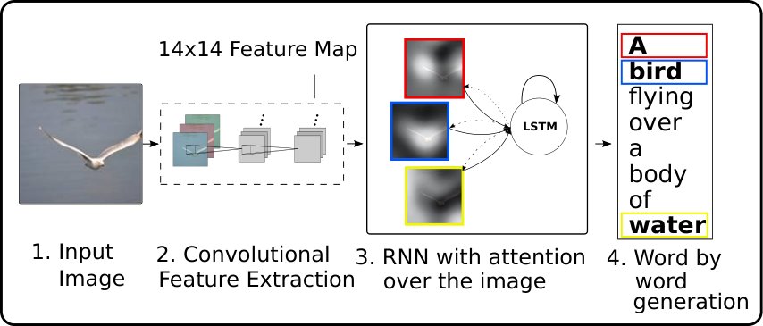
Figure 1: Our model learns a words/image alignment. The visualized attentional maps (3) are explained in section 3.1 & 5.4
图 1:我们的模型学习词与图像的对齐。可视化的注意力图(3)在第 3.1 节与第 5.4 节解释。
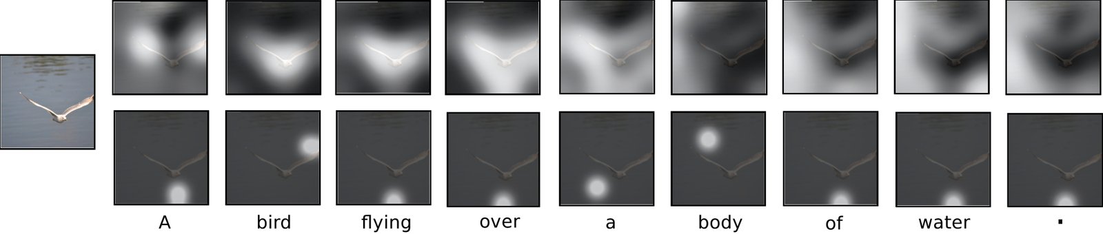
Figure 2: Attention over time. As the model generates each word, its attention changes to reflect the relevant parts of the image. “soft” (top row) vs “hard” (bottom row) attention. (Note that both models generated the same captions in this example.)
图 2:随时间变化的注意力。模型每生成一个词,注意力就会转到图像中相关的部分。上一行是“软”注意力,下一行是“硬”注意力。(注意本例中两个模型生成了相同的描述。)
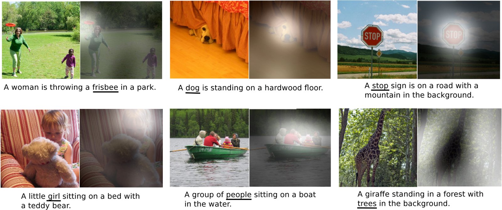
Figure 3: Examples of attending to the correct object (white indicates the attended regions, underlines indicated the corresponding word)
图 3:注意到正确物体的例子(白色表示被注意的区域,下划线标出对应的词)
One of the most curious facets of the human visual system is the presence of attention (Rensink, 2000; Corbetta & Shulman, 2002). Rather than compress an entire image into a static representation, attention allows for salient features to dynamically come to the forefront as needed. This is especially important when there is a lot of clutter in an image. Using representations (such as those from the top layer of a convnet) that distill information in image down to the most salient objects is one effective solution that has been widely adopted in previous work. Unfortunately, this has one potential drawback of losing information which could be useful for richer, more descriptive captions. Using more low-level representation can help preserve this information. However working with these features necessitates a powerful mechanism to steer the model to information important to the task at hand.
人类视觉系统最令人好奇的特点之一,就是注意力的存在(Rensink,2000;Corbetta 与 Shulman,2002)。注意力不是把整张图压成一个静态表示,而是让显著特征在需要时动态走到前台。图像很杂乱时,这一点尤为重要。用卷积网络顶层这类表示,把图像信息提炼到最显著的物体,是以往工作广泛采用的有效办法。可惜它有一个潜在缺点:可能丢掉对更丰富、更细致描述有用的信息。使用更低层的表示有助于保留这些信息。但要处理这些特征,就需要一种有力的机制,把模型引导到当前任务真正重要的信息上。
In this paper, we describe approaches to caption generation that attempt to incorporate a form of attention with two variants: a “hard” attention mechanism and a “soft” attention mechanism. We also show how one advantage of including attention is the ability to visualize what the model “sees”. Encouraged by recent advances in caption generation and inspired by recent success in employing attention in machine translation (Bahdanau et al., 2014) and object recognition (Ba et al., 2014; Mnih et al., 2014), we investigate models that can attend to salient part of an image while generating its caption.
本文描述的描述生成方法试图引入一种注意力,并给出两个变体:“硬”注意力机制与“软”注意力机制。我们还说明,加入注意力的一个好处是能够可视化模型“看见”了什么。受近期描述生成进展的鼓舞,并受到机器翻译(Bahdanau 等,2014)与物体识别(Ba 等,2014;Mnih 等,2014)中注意力成功应用的启发,我们研究能在生成描述时注视图像显著部分的模型。
The contributions of this paper are the following:
本文贡献如下:
- • We introduce two attention-based image caption generators under a common framework (Sec. 3.1): 1) a “soft” deterministic attention mechanism trainable by standard back-propagation methods and 2) a “hard” stochastic attention mechanism trainable by maximizing an approximate variational lower bound or equivalently by REINFORCE (Williams, 1992).
- • 我们在同一框架下引入两种基于注意力的图像描述生成器(第 3.1 节):1)可用标准反向传播训练的“软”确定性注意力机制;2)通过最大化近似变分下界(或等价地用 REINFORCE(Williams,1992))训练的“硬”随机注意力机制。
- • We show how we can gain insight and interpret the results of this framework by visualizing “where” and “what” the attention focused on. (see Sec. 5.4)
- • 我们展示如何通过可视化注意力聚焦在“何处”以及“何物”,来理解并解释该框架的结果。(见第 5.4 节)
- • Finally, we quantitatively validate the usefulness of attention in caption generation with state of the art performance (Sec. 5.3) on three benchmark datasets: Flickr8k (Hodosh et al., 2013) , Flickr30k (Young et al., 2014) and the MS COCO dataset (Lin et al., 2014).
- • 最后,我们在三个基准数据集上用当时最优表现定量验证注意力对描述生成的用处(第 5.3 节):Flickr8k(Hodosh 等,2013)、Flickr30k(Young 等,2014)以及 MS COCO 数据集(Lin 等,2014)。
2 Related Work
2 相关工作
In this section we provide relevant background on previous work on image caption generation and attention. Recently, several methods have been proposed for generating image descriptions. Many of these methods are based on recurrent neural networks and inspired by the successful use of sequence to sequence training with neural networks for machine translation (Cho et al., 2014; Bahdanau et al., 2014; Sutskever et al., 2014). One major reason image caption generation is well suited to the encoder-decoder framework (Cho et al., 2014) of machine translation is because it is analogous to “translating” an image to a sentence.
本节给出图像描述生成与注意力方面的相关背景。近期已有多种生成图像描述的方法。其中许多基于循环神经网络,并受到机器翻译中序列到序列神经网络训练成功应用的启发(Cho 等,2014;Bahdanau 等,2014;Sutskever 等,2014)。描述生成很适合机器翻译的编码器–解码器框架(Cho 等,2014),一个主要原因是它类似于把图像“翻译”成句子。
The first approach to use neural networks for caption generation was Kiros et al. (2014a), who proposed a multimodal log-bilinear model that was biased by features from the image. This work was later followed by Kiros et al. (2014b) whose method was designed to explicitly allow a natural way of doing both ranking and generation. Mao et al. (2014) took a similar approach to generation but replaced a feed-forward neural language model with a recurrent one. Both Vinyals et al. (2014) and Donahue et al. (2014) use LSTM RNNs for their models. Unlike Kiros et al. (2014a) and Mao et al. (2014) whose models see the image at each time step of the output word sequence, Vinyals et al. (2014) only show the image to the RNN at the beginning. Along with images, Donahue et al. (2014) also apply LSTMs to videos, allowing their model to generate video descriptions.
最早把神经网络用于描述生成的是 Kiros 等(2014a),他们提出一种由图像特征偏置的多模态对数双线性模型。随后 Kiros 等(2014b)的方法被设计成能自然地同时做排序与生成。Mao 等(2014)采取类似的生成思路,但用循环神经语言模型替换了前馈语言模型。Vinyals 等(2014)与 Donahue 等(2014)都在模型中使用 LSTM RNN。与 Kiros 等(2014a)和 Mao 等(2014)在输出词序列的每一步都看到图像不同,Vinyals 等(2014)只在开始时把图像交给 RNN。除图像外,Donahue 等(2014)还把 LSTM 用到视频上,使模型能够生成视频描述。
All of these works represent images as a single feature vector from the top layer of a pre-trained convolutional network. Karpathy & Li (2014) instead proposed to learn a joint embedding space for ranking and generation whose model learns to score sentence and image similarity as a function of R-CNN object detections with outputs of a bidirectional RNN. Fang et al. (2014) proposed a three-step pipeline for generation by incorporating object detections. Their model first learn detectors for several visual concepts based on a multi-instance learning framework. A language model trained on captions was then applied to the detector outputs, followed by rescoring from a joint image-text embedding space. Unlike these models, our proposed attention framework does not explicitly use object detectors but instead learns latent alignments from scratch. This allows our model to go beyond “objectness” and learn to attend to abstract concepts.
这些工作都把图像表示成预训练卷积网络顶层的单个特征向量。Karpathy 与 Li(2014)则提出学习一个用于排序与生成的联合嵌入空间,其模型根据 R-CNN 物体检测与双向 RNN 的输出,给句子与图像的相似度打分。Fang 等(2014)提出三步生成流程,引入物体检测:模型先在多实例学习框架下学习若干视觉概念的检测器,再把检测器输出送入在描述上训练的语言模型,最后用联合图文嵌入空间重打分。与这些模型不同,我们提出的注意力框架并不显式使用物体检测器,而是从零开始学习潜在对齐。这使模型可以超越“物体性”,学会注意抽象概念。
Prior to the use of neural networks for generating captions, two main approaches were dominant. The first involved generating caption templates which were filled in based on the results of object detections and attribute discovery (Kulkarni et al. (2013), Li et al. (2011), Yang et al. (2011), Mitchell et al. (2012), Elliott & Keller (2013)). The second approach was based on first retrieving similar captioned images from a large database then modifying these retrieved captions to fit the query (Kuznetsova et al., 2012; Kuznetsova et al., 2014). These approaches typically involved an intermediate “generalization” step to remove the specifics of a caption that are only relevant to the retrieved image, such as the name of a city. Both of these approaches have since fallen out of favour to the now dominant neural network methods.
在用神经网络生成描述之前,主流大致有两类方法。第一类是生成描述模板,再根据物体检测与属性发现的结果填空(Kulkarni 等(2013),Li 等(2011),Yang 等(2011),Mitchell 等(2012),Elliott 与 Keller(2013))。第二类是先从大型数据库中检索相似的带描述图像,再修改这些检索到的描述以适配查询(Kuznetsova 等,2012;Kuznetsova 等,2014)。这类方法通常还需要一步中间的“泛化”,去掉只与被检索图像相关的细节,例如城市名。这两类方法后来都让位于如今占主导的神经网络方法。
There has been a long line of previous work incorporating attention into neural networks for vision related tasks. Some that share the same spirit as our work include Larochelle & Hinton (2010); Denil et al. (2012); Tang et al. (2014). In particular however, our work directly extends the work of Bahdanau et al. (2014); Mnih et al. (2014); Ba et al. (2014).
把注意力引入视觉相关神经网络已有很长的研究脉络。与我们工作精神相近的包括 Larochelle 与 Hinton(2010);Denil 等(2012);Tang 等(2014)。不过,本文直接延伸的是 Bahdanau 等(2014);Mnih 等(2014);Ba 等(2014)的工作。
3 Image Caption Generation with Attention Mechanism
3 带注意力机制的图像描述生成
3.1 Model Details
3.1 模型细节
In this section, we describe the two variants of our attention-based model by first describing their common framework. The main difference is the definition of the function which we describe in detail in Section 4. We denote vectors with bolded font and matrices with capital letters. In our description below, we suppress bias terms for readability.
本节先描述两种基于注意力的模型变体的共同框架。主要差别在于 函数的定义,我们在第 4 节详细说明。向量用粗体,矩阵用大写字母。为便于阅读,下面的描述略去偏置项。
3.1.1 Encoder: Convolutional Features
Our model takes a single raw image and generates a caption encoded as a sequence of 1-of- encoded words.
3.1.1 编码器:卷积特征
我们的模型接收一张原始图像,并生成描述 ,它被编码为一串 1-of- 的词。
where is the size of the vocabulary and is the length of the caption.
其中 是词表大小, 是描述长度。
We use a convolutional neural network in order to extract a set of feature vectors which we refer to as annotation vectors. The extractor produces vectors, each of which is a D-dimensional representation corresponding to a part of the image.
我们用卷积神经网络提取一组特征向量,称为标注向量。提取器产生 个向量,每个都是对应图像某一部分的 维表示。
In order to obtain a correspondence between the feature vectors and portions of the 2-D image, we extract features from a lower convolutional layer unlike previous work which instead used a fully connected layer. This allows the decoder to selectively focus on certain parts of an image by selecting a subset of all the feature vectors.
为了让特征向量与二维图像的各个部分对应起来,我们从较低的卷积层提取特征,而不是像以往工作那样使用全连接层。这样,解码器可以通过选择特征向量子集,有选择地聚焦图像的某些部分。
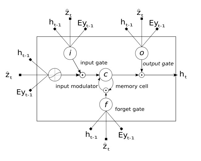
Figure 4: A LSTM cell, lines with bolded squares imply projections with a learnt weight vector. Each cell learns how to weigh its input components (input gate), while learning how to modulate that contribution to the memory (input modulator). It also learns weights which erase the memory cell (forget gate), and weights which control how this memory should be emitted (output gate).
图 4:一个 LSTM 单元,带粗方框的线表示带可学习权重向量的投影。每个单元学习如何权衡其输入分量(输入门),同时学习如何调节该贡献写入记忆(输入调制器)。它还学习擦除记忆单元的权重(遗忘门),以及控制这段记忆如何输出的权重(输出门)。
3.1.2 Decoder: Long Short-Term Memory Network
We use a long short-term memory (LSTM) network (Hochreiter & Schmidhuber, 1997) that produces a caption by generating one word at every time step conditioned on a context vector, the previous hidden state and the previously generated words. Our implementation of LSTM closely follows the one used in Zaremba et al. (2014) (see Fig. 4). Using to denote a simple affine transformation with parameters that are learned,
3.1.2 解码器:长短期记忆网络
我们使用长短期记忆(LSTM)网络(Hochreiter 与 Schmidhuber,1997),它在每一步根据上下文向量、上一隐藏状态以及此前生成的词,生成描述中的一个词。我们的 LSTM 实现紧密沿用 Zaremba 等(2014)的做法(见图 4)。用 表示带可学习参数的简单仿射变换,
$$\displaystyle\begin{pmatrix}\mathbf{i}{t}\
\mathbf{f}{t}\
\mathbf{o}{t}\
\mathbf{g}{t}\
\end{pmatrix}= \ \displaystyle\begin{pmatrix}\sigma\
\sigma\
\sigma\
\tanh\
\end{pmatrix}T_{D+m+n,n}\begin{pmatrix}\mathbf{E}\mathbf{y}{t-1}\
\mathbf{h}{t-1}\
\hat{\mathbf{z}{t}}\
\end{pmatrix} \ \displaystyle\mathbf{c}{t} \ \displaystyle=\mathbf{f}{t}\odot\mathbf{c}{t-1}+\mathbf{i}{t}\odot\mathbf{g}{t} \ \displaystyle\mathbf{h}{t} \ \displaystyle=\mathbf{o}{t}\odot\tanh(\mathbf{c}_{t}). \tag{1}$$
Here, , , , , are the input, forget, memory, output and hidden state of the LSTM, respectively. The vector is the context vector, capturing the visual information associated with a particular input location, as explained below. is an embedding matrix. Let and denote the embedding and LSTM dimensionality respectively and and be the logistic sigmoid activation and element-wise multiplication respectively.
这里,、、、、 分别是 LSTM 的输入、遗忘、记忆、输出与隐藏状态。向量 是上下文向量,捕捉与特定输入位置相关的视觉信息,下文说明。 是嵌入矩阵。令 与 分别表示嵌入维数与 LSTM 维数, 与 分别是 logistic sigmoid 激活与逐元素乘法。
In simple terms, the context vector (equations (1)–(3)) is a dynamic representation of the relevant part of the image input at time . We define a mechanism that computes from the annotation vectors corresponding to the features extracted at different image locations. For each location , the mechanism generates a positive weight which can be interpreted either as the probability that location is the right place to focus for producing the next word (the “hard” but stochastic attention mechanism), or as the relative importance to give to location in blending the ’s together. The weight of each annotation vector is computed by an attention model for which we use a multilayer perceptron conditioned on the previous hidden state . The soft version of this attention mechanism was introduced by Bahdanau et al. (2014). For emphasis, we note that the hidden state varies as the output RNN advances in its output sequence: “where” the network looks next depends on the sequence of words that has already been generated.
简单来说,上下文向量 (式(1)–(3))是时刻 与图像输入相关部分对应的动态表示。我们定义机制 ,从对应于不同图像位置所提特征的标注向量 计算 。对每个位置 ,该机制生成一个正权重 :它既可以解释为“位置 是生成下一个词时该注视之处”的概率(“硬”但随机的注意力机制),也可以解释为把各个 混合时赋予位置 的相对重要性。每个标注向量 的权重 由注意力模型 计算,我们用一个以先前隐藏状态 为条件的多层感知机来实现。这种注意力机制的软版本由 Bahdanau 等(2014)引入。需要强调的是,隐藏状态会随着输出 RNN 在输出序列上推进而变化:网络接下来看“哪里”,取决于已经生成的词序列。
Once the weights (which sum to one) are computed, the context vector is computed by
权重(和为 1)计算完成后,上下文向量 由下式得到
where is a function that returns a single vector given the set of annotation vectors and their corresponding weights. The details of function are discussed in Sec. 4.
其中 根据一组标注向量及其对应权重返回单个向量。 函数的细节在第 4 节讨论。
The initial memory state and hidden state of the LSTM are predicted by an average of the annotation vectors fed through two separate MLPs (init,c and init,h):
LSTM 的初始记忆状态与隐藏状态,由标注向量的平均分别通过两个 MLP(init,c 与 init,h)来预测:
In this work, we use a deep output layer (Pascanu et al., 2014) to compute the output word probability given the LSTM state, the context vector and the previous word:
本文用深层输出层(Pascanu 等,2014),根据 LSTM 状态、上下文向量以及前一个词来计算输出词概率:
Where , , , and are learned parameters initialized randomly.
其中 、、 以及 都是随机初始化的可学习参数。
4 Learning Stochastic “Hard” vs Deterministic “Soft” Attention
4 学习随机“硬”注意力与确定性“软”注意力
In this section we discuss two alternative mechanisms for the attention model : stochastic attention and deterministic attention.
本节讨论注意力模型 的两种替代机制:随机注意力与确定性注意力。
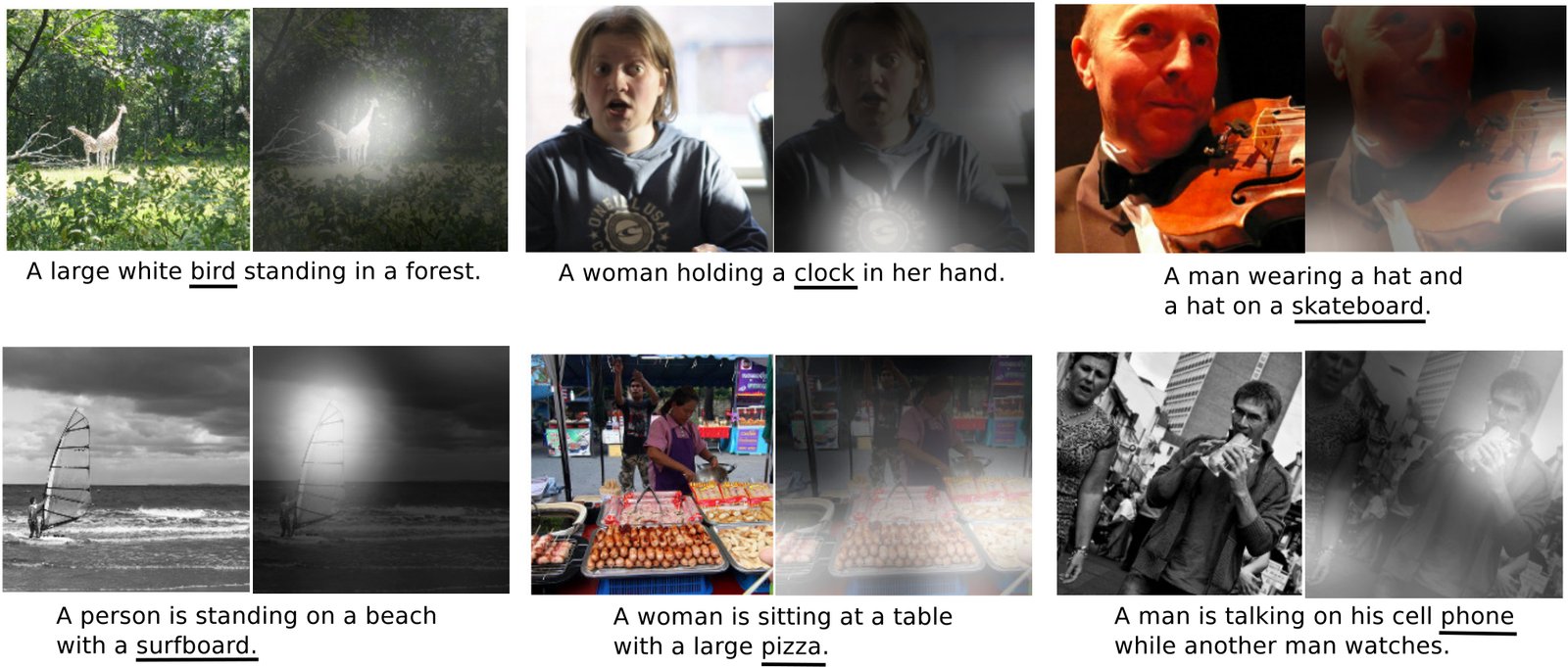
Figure 5: Examples of mistakes where we can use attention to gain intuition into what the model saw.
图 5:一些错误例子,我们可以借助注意力来直觉地理解模型当时看见了什么。
4.1 Stochastic “Hard” Attention
4.1 随机“硬”注意力
We represent the location variable as where the model decides to focus attention when generating the word. is an indicator one-hot variable which is set to 1 if the -th location (out of ) is the one used to extract visual features. By treating the attention locations as intermediate latent variables, we can assign a multinoulli distribution parametrized by , and view as a random variable:
我们用位置变量 表示模型在生成第 个词时决定把注意力放在哪里。 是一个指示独热变量:若第 个位置(共 个)被用来提取视觉特征,则取 1。把注意力位置当作中间隐变量,我们可以赋予由 参数化的多项伯努利分布,并把 视为随机变量:
We define a new objective function that is a variational lower bound on the marginal log-likelihood of observing the sequence of words given image features . The learning algorithm for the parameters of the models can be derived by directly optimizing :
我们定义新的目标函数 ,它是在给定图像特征 时观察到词序列 的边际对数似然 的变分下界。模型参数 的学习算法可以通过直接优化 导出:
$$\frac{\partial L_{s}}{\partial W}=\sum_{s}p(s\mid\mathbf{a})\bigg[\frac{\partial\log p(\mathbf{y}\mid s,\mathbf{a})}{\partial W}+\
\log p(\mathbf{y}\mid s,\mathbf{a})\frac{\partial\log p(s\mid\mathbf{a})}{\partial W}\bigg]. \tag{11}$$
Equation 11 suggests a Monte Carlo based sampling approximation of the gradient with respect to the model parameters. This can be done by sampling the location from a multinouilli distribution defined by Equation 8.
式 11 表明,可以用基于蒙特卡洛采样的方法来近似对模型参数的梯度。做法是按式 8 定义的多项伯努利分布采样位置 。
$$\frac{\partial L_{s}}{\partial W}\approx\frac{1}{N}\sum_{n=1}^{N}\bigg[\frac{\partial\log p(\mathbf{y}\mid\tilde{s}^{n},\mathbf{a})}{\partial W}+\
\log p(\mathbf{y}\mid\tilde{s}^{n},\mathbf{a})\frac{\partial\log p(\tilde{s}^{n}\mid\mathbf{a})}{\partial W}\bigg] \tag{12}$$
A moving average baseline is used to reduce the variance in the Monte Carlo estimator of the gradient, following Weaver & Tao (2001). Similar, but more complicated variance reduction techniques have previously been used by Mnih et al. (2014) and Ba et al. (2014). Upon seeing the mini-batch, the moving average baseline is estimated as an accumulated sum of the previous log likelihoods with exponential decay:
为降低梯度蒙特卡洛估计的方差,我们沿用 Weaver 与 Tao(2001)使用滑动平均基线。Mnih 等(2014)与 Ba 等(2014)曾使用类似但更复杂的方差削减技术。看到第 个小批次时,滑动平均基线按此前对数似然的指数衰减累加来估计:
To further reduce the estimator variance, an entropy term on the multinouilli distribution is added. Also, with probability 0.5 for a given image, we set the sampled attention location to its expected value . Both techniques improve the robustness of the stochastic attention learning algorithm. The final learning rule for the model is then the following:
为进一步降低估计方差,还加入多项伯努利分布上的熵项 。此外,对给定图像以 0.5 的概率把采样到的注意力位置 设成其期望值 。两种技术都提高了随机注意力学习算法的稳健性。模型最终的学习规则如下:
$$\frac{\partial L_{s}}{\partial W}\approx\frac{1}{N}\sum_{n=1}^{N}\bigg[\frac{\partial\log p(\mathbf{y}\mid\tilde{s}^{n},\mathbf{a})}{\partial W}+\
\lambda_{r}(\log p(\mathbf{y}\mid\tilde{s}^{n},\mathbf{a})-b)\frac{\partial\log p(\tilde{s}^{n}\mid\mathbf{a})}{\partial W}+\lambda_{e}\frac{\partial H[\tilde{s}^{n}]}{\partial W}\bigg] \tag{13}$$
where, and are two hyper-parameters set by cross-validation. As pointed out and used in Ba et al. (2014) and Mnih et al. (2014), this is formulation is equivalent to the REINFORCE learning rule (Williams, 1992), where the reward for the attention choosing a sequence of actions is a real value proportional to the log likelihood of the target sentence under the sampled attention trajectory.
其中 与 是由交叉验证设定的两个超参数。正如 Ba 等(2014)与 Mnih 等(2014)所指出并采用的,这一形式等价于 REINFORCE 学习规则(Williams,1992):注意力选择一系列动作的奖励,是与目标句子在采样注意力轨迹下的对数似然成正比的实值。
In making a hard choice at every point, from Equation 6 is a function that returns a sampled at every point in time based upon a multinouilli distribution parameterized by .
由于每一步都做硬选择,式 6 中的 是一个函数:它在每一时刻根据由 参数化的多项伯努利分布,返回一个采样得到的 。
4.2 Deterministic “Soft” Attention
4.2 确定性“软”注意力
Learning stochastic attention requires sampling the attention location each time, instead we can take the expectation of the context vector directly,
学习随机注意力需要每次采样注意力位置 ,我们也可以直接取上下文向量 的期望,
and formulate a deterministic attention model by computing a soft attention weighted annotation vector as introduced by Bahdanau et al. (2014). This corresponds to feeding in a soft weighted context into the system. The whole model is smooth and differentiable under the deterministic attention, so learning end-to-end is trivial by using standard back-propagation.
并按 Bahdanau 等(2014)引入的方式,用软注意力加权的标注向量 来构成确定性注意力模型。这相当于把经 软加权的上下文送入系统。在确定性注意力下整个模型光滑可微,用标准反向传播即可端到端学习。
Learning the deterministic attention can also be understood as approximately optimizing the marginal likelihood in Equation 10 under the attention location random variable from Sec. 4.1. The hidden activation of LSTM is a linear projection of the stochastic context vector followed by non-linearity. To the first order Taylor approximation, the expected value is equal to computing using a single forward prop with the expected context vector . Considering Eq. 7, let , denotes computed by setting the random variable value to . We define the normalized weighted geometric mean for the softmax word prediction:
学习确定性注意力也可以理解为:在第 4.1 节的注意力位置随机变量 下,近似优化式 10 中的边际似然。LSTM 的隐藏激活 是随机上下文向量 的线性投影再接 非线性。按一阶泰勒近似,期望 等于用期望上下文向量 做一次前向计算得到的 。考虑式 7,令 , 表示把随机变量 取成 时算出的 。我们为 softmax 第 个词的预测定义归一化加权几何平均:
The equation above shows the normalized weighted geometric mean of the caption prediction can be approximated well by using the expected context vector, where . It shows that the NWGM of a softmax unit is obtained by applying softmax to the expectations of the underlying linear projections. Also, from the results in Baldi & Sadowski (2014), under softmax activation. That means the expectation of the outputs over all possible attention locations induced by random variable is computed by simple feedforward propagation with expected context vector . In other words, the deterministic attention model is an approximation to the marginal likelihood over the attention locations.
上式表明,描述预测的归一化加权几何平均可以用期望上下文向量很好地近似,其中 。这说明 softmax 单元的 NWGM,是对底层线性投影的期望再做 softmax 得到的。此外,根据 Baldi 与 Sadowski(2014)的结果,在 softmax 激活下有 。也就是说,对随机变量 诱导的所有可能注意力位置,输出的期望可以通过用期望上下文向量 做一次简单前馈计算得到。换句话说,确定性注意力模型是对注意力位置边际似然的一种近似。
4.2.1 Doubly Stochastic Attention
By construction, as they are the output of a softmax. In training the deterministic version of our model we introduce a form of doubly stochastic regularization, where we also encourage . This can be interpreted as encouraging the model to pay equal attention to every part of the image over the course of generation. In our experiments, we observed that this penalty was important quantitatively to improving overall BLEU score and that qualitatively this leads to more rich and descriptive captions. In addition, the soft attention model predicts a gating scalar from previous hidden state at each time step , such that, , where . We notice our attention weights put more emphasis on the objects in the images by including the scalar .
4.2.1 双重随机注意力
由构造可知,,因为它们是 softmax 的输出。在训练模型的确定性版本时,我们引入一种双重随机正则:还鼓励 。这可以理解为鼓励模型在整段生成过程中对图像各部分给予大致均等的注意。实验中我们观察到,这一惩罚在定量上对提高总体 BLEU 很重要,在定性上也带来更丰富、更细致的描述。此外,软注意力模型在每一时刻 还从先前隐藏状态 预测一个门控标量 ,使得 ,其中 。我们注意到,加入标量 后,注意力权重更强调图像中的物体。
| BLEU | |||||||||||||||||||||||||||||||||||||||||||||||||
|---|---|---|---|---|---|---|---|---|---|---|---|---|---|---|---|---|---|---|---|---|---|---|---|---|---|---|---|---|---|---|---|---|---|---|---|---|---|---|---|---|---|---|---|---|---|---|---|---|---|
| Dataset | Model | BLEU-1 | BLEU-2 | BLEU-3 | BLEU-4 | METEOR | |||||||||||||||||||||||||||||||||||||||||||
| Flickr8k | Google NIC(Vinyals et al., 2014)†Σ Log Bilinear (Kiros et al., 2014a)∘ Soft-Attention Hard-Attention | Google NIC(Vinyals et al., 2014)†Σ | Log Bilinear (Kiros et al., 2014a)∘ | Soft-Attention | Hard-Attention | 63 65.6 67 67 | 63 | 65.6 | 67 | 67 | 41 42.4 44.8 45.7 | 41 | 42.4 | 44.8 | 45.7 | 27 27.7 29.9 31.4 | 27 | 27.7 | 29.9 | 31.4 | — 17.7 19.5 21.3 | — | 17.7 | 19.5 | 21.3 | — 17.31 18.93 20.30 | — | 17.31 | 18.93 | 20.30 | |||||||||||||||||||
| Google NIC(Vinyals et al., 2014)†Σ | |||||||||||||||||||||||||||||||||||||||||||||||||
| Log Bilinear (Kiros et al., 2014a)∘ | |||||||||||||||||||||||||||||||||||||||||||||||||
| Soft-Attention | |||||||||||||||||||||||||||||||||||||||||||||||||
| Hard-Attention | |||||||||||||||||||||||||||||||||||||||||||||||||
| 63 | |||||||||||||||||||||||||||||||||||||||||||||||||
| 65.6 | |||||||||||||||||||||||||||||||||||||||||||||||||
| 67 | |||||||||||||||||||||||||||||||||||||||||||||||||
| 67 | |||||||||||||||||||||||||||||||||||||||||||||||||
| 41 | |||||||||||||||||||||||||||||||||||||||||||||||||
| 42.4 | |||||||||||||||||||||||||||||||||||||||||||||||||
| 44.8 | |||||||||||||||||||||||||||||||||||||||||||||||||
| 45.7 | |||||||||||||||||||||||||||||||||||||||||||||||||
| 27 | |||||||||||||||||||||||||||||||||||||||||||||||||
| 27.7 | |||||||||||||||||||||||||||||||||||||||||||||||||
| 29.9 | |||||||||||||||||||||||||||||||||||||||||||||||||
| 31.4 | |||||||||||||||||||||||||||||||||||||||||||||||||
| — | |||||||||||||||||||||||||||||||||||||||||||||||||
| 17.7 | |||||||||||||||||||||||||||||||||||||||||||||||||
| 19.5 | |||||||||||||||||||||||||||||||||||||||||||||||||
| 21.3 | |||||||||||||||||||||||||||||||||||||||||||||||||
| — | |||||||||||||||||||||||||||||||||||||||||||||||||
| 17.31 | |||||||||||||||||||||||||||||||||||||||||||||||||
| 18.93 | |||||||||||||||||||||||||||||||||||||||||||||||||
| 20.30 | |||||||||||||||||||||||||||||||||||||||||||||||||
| Flickr30k | Google NIC†∘Σ Log Bilinear Soft-Attention Hard-Attention | Google NIC†∘Σ | Log Bilinear | Soft-Attention | Hard-Attention | 66.3 60.0 66.7 66.9 | 66.3 | 60.0 | 66.7 | 66.9 | 42.3 38 43.4 43.9 | 42.3 | 38 | 43.4 | 43.9 | 27.7 25.4 28.8 29.6 | 27.7 | 25.4 | 28.8 | 29.6 | 18.3 17.1 19.1 19.9 | 18.3 | 17.1 | 19.1 | 19.9 | — 16.88 18.49 18.46 | — | 16.88 | 18.49 | 18.46 | |||||||||||||||||||
| Google NIC†∘Σ | |||||||||||||||||||||||||||||||||||||||||||||||||
| Log Bilinear | |||||||||||||||||||||||||||||||||||||||||||||||||
| Soft-Attention | |||||||||||||||||||||||||||||||||||||||||||||||||
| Hard-Attention | |||||||||||||||||||||||||||||||||||||||||||||||||
| 66.3 | |||||||||||||||||||||||||||||||||||||||||||||||||
| 60.0 | |||||||||||||||||||||||||||||||||||||||||||||||||
| 66.7 | |||||||||||||||||||||||||||||||||||||||||||||||||
| 66.9 | |||||||||||||||||||||||||||||||||||||||||||||||||
| 42.3 | |||||||||||||||||||||||||||||||||||||||||||||||||
| 38 | |||||||||||||||||||||||||||||||||||||||||||||||||
| 43.4 | |||||||||||||||||||||||||||||||||||||||||||||||||
| 43.9 | |||||||||||||||||||||||||||||||||||||||||||||||||
| 27.7 | |||||||||||||||||||||||||||||||||||||||||||||||||
| 25.4 | |||||||||||||||||||||||||||||||||||||||||||||||||
| 28.8 | |||||||||||||||||||||||||||||||||||||||||||||||||
| 29.6 | |||||||||||||||||||||||||||||||||||||||||||||||||
| 18.3 | |||||||||||||||||||||||||||||||||||||||||||||||||
| 17.1 | |||||||||||||||||||||||||||||||||||||||||||||||||
| 19.1 | |||||||||||||||||||||||||||||||||||||||||||||||||
| 19.9 | |||||||||||||||||||||||||||||||||||||||||||||||||
| — | |||||||||||||||||||||||||||||||||||||||||||||||||
| 16.88 | |||||||||||||||||||||||||||||||||||||||||||||||||
| 18.49 | |||||||||||||||||||||||||||||||||||||||||||||||||
| 18.46 | |||||||||||||||||||||||||||||||||||||||||||||||||
| COCO | CMU/MS Research (Chen & Zitnick, 2014)a MS Research (Fang et al., 2014)†a BRNN (Karpathy & Li, 2014)∘ Google NIC†∘Σ Log Bilinear∘ Soft-Attention Hard-Attention | CMU/MS Research (Chen & Zitnick, 2014)a | MS Research (Fang et al., 2014)†a | BRNN (Karpathy & Li, 2014)∘ | Google NIC†∘Σ | Log Bilinear∘ | Soft-Attention | Hard-Attention | — — 64.2 66.6 70.8 70.7 71.8 | — | — | 64.2 | 66.6 | 70.8 | 70.7 | 71.8 | — — 45.1 46.1 48.9 49.2 50.4 | — | — | 45.1 | 46.1 | 48.9 | 49.2 | 50.4 | — — 30.4 32.9 34.4 34.4 35.7 | — | — | 30.4 | 32.9 | 34.4 | 34.4 | 35.7 | — — 20.3 24.6 24.3 24.3 25.0 | — | — | 20.3 | 24.6 | 24.3 | 24.3 | 25.0 | 20.41 20.71 — — 20.03 23.90 23.04 | 20.41 | 20.71 | — | — | 20.03 | 23.90 | 23.04 | |
| CMU/MS Research (Chen & Zitnick, 2014)a | |||||||||||||||||||||||||||||||||||||||||||||||||
| MS Research (Fang et al., 2014)†a | |||||||||||||||||||||||||||||||||||||||||||||||||
| BRNN (Karpathy & Li, 2014)∘ | |||||||||||||||||||||||||||||||||||||||||||||||||
| Google NIC†∘Σ | |||||||||||||||||||||||||||||||||||||||||||||||||
| Log Bilinear∘ | |||||||||||||||||||||||||||||||||||||||||||||||||
| Soft-Attention | |||||||||||||||||||||||||||||||||||||||||||||||||
| Hard-Attention | |||||||||||||||||||||||||||||||||||||||||||||||||
| — | |||||||||||||||||||||||||||||||||||||||||||||||||
| — | |||||||||||||||||||||||||||||||||||||||||||||||||
| 64.2 | |||||||||||||||||||||||||||||||||||||||||||||||||
| 66.6 | |||||||||||||||||||||||||||||||||||||||||||||||||
| 70.8 | |||||||||||||||||||||||||||||||||||||||||||||||||
| 70.7 | |||||||||||||||||||||||||||||||||||||||||||||||||
| 71.8 | |||||||||||||||||||||||||||||||||||||||||||||||||
| — | |||||||||||||||||||||||||||||||||||||||||||||||||
| — | |||||||||||||||||||||||||||||||||||||||||||||||||
| 45.1 | |||||||||||||||||||||||||||||||||||||||||||||||||
| 46.1 | |||||||||||||||||||||||||||||||||||||||||||||||||
| 48.9 | |||||||||||||||||||||||||||||||||||||||||||||||||
| 49.2 | |||||||||||||||||||||||||||||||||||||||||||||||||
| 50.4 | |||||||||||||||||||||||||||||||||||||||||||||||||
| — | |||||||||||||||||||||||||||||||||||||||||||||||||
| — | |||||||||||||||||||||||||||||||||||||||||||||||||
| 30.4 | |||||||||||||||||||||||||||||||||||||||||||||||||
| 32.9 | |||||||||||||||||||||||||||||||||||||||||||||||||
| 34.4 | |||||||||||||||||||||||||||||||||||||||||||||||||
| 34.4 | |||||||||||||||||||||||||||||||||||||||||||||||||
| 35.7 | |||||||||||||||||||||||||||||||||||||||||||||||||
| — | |||||||||||||||||||||||||||||||||||||||||||||||||
| — | |||||||||||||||||||||||||||||||||||||||||||||||||
| 20.3 | |||||||||||||||||||||||||||||||||||||||||||||||||
| 24.6 | |||||||||||||||||||||||||||||||||||||||||||||||||
| 24.3 | |||||||||||||||||||||||||||||||||||||||||||||||||
| 24.3 | |||||||||||||||||||||||||||||||||||||||||||||||||
| 25.0 | |||||||||||||||||||||||||||||||||||||||||||||||||
| 20.41 | |||||||||||||||||||||||||||||||||||||||||||||||||
| 20.71 | |||||||||||||||||||||||||||||||||||||||||||||||||
| — | |||||||||||||||||||||||||||||||||||||||||||||||||
| — | |||||||||||||||||||||||||||||||||||||||||||||||||
| 20.03 | |||||||||||||||||||||||||||||||||||||||||||||||||
| 23.90 | |||||||||||||||||||||||||||||||||||||||||||||||||
| 23.04 |
| Google NIC(Vinyals et al., 2014)†Σ |
|---|
| Log Bilinear (Kiros et al., 2014a)∘ |
| Soft-Attention |
| Hard-Attention |
| 63 |
|---|
| 65.6 |
| 67 |
| 67 |
| 41 |
|---|
| 42.4 |
| 44.8 |
| 45.7 |
| 27 |
|---|
| 27.7 |
| 29.9 |
| 31.4 |
| — |
|---|
| 17.7 |
| 19.5 |
| 21.3 |
| — |
|---|
| 17.31 |
| 18.93 |
| 20.30 |
| Google NIC†∘Σ |
|---|
| Log Bilinear |
| Soft-Attention |
| Hard-Attention |
| 66.3 |
|---|
| 60.0 |
| 66.7 |
| 66.9 |
| 42.3 |
|---|
| 38 |
| 43.4 |
| 43.9 |
| 27.7 |
|---|
| 25.4 |
| 28.8 |
| 29.6 |
| 18.3 |
|---|
| 17.1 |
| 19.1 |
| 19.9 |
| — |
|---|
| 16.88 |
| 18.49 |
| 18.46 |
| CMU/MS Research (Chen & Zitnick, 2014)a |
|---|
| MS Research (Fang et al., 2014)†a |
| BRNN (Karpathy & Li, 2014)∘ |
| Google NIC†∘Σ |
| Log Bilinear∘ |
| Soft-Attention |
| Hard-Attention |
| — |
|---|
| — |
| 64.2 |
| 66.6 |
| 70.8 |
| 70.7 |
| 71.8 |
| — |
|---|
| — |
| 45.1 |
| 46.1 |
| 48.9 |
| 49.2 |
| 50.4 |
| — |
|---|
| — |
| 30.4 |
| 32.9 |
| 34.4 |
| 34.4 |
| 35.7 |
| — |
|---|
| — |
| 20.3 |
| 24.6 |
| 24.3 |
| 24.3 |
| 25.0 |
| 20.41 |
|---|
| 20.71 |
| — |
| — |
| 20.03 |
| 23.90 |
| 23.04 |
Table 1: BLEU-1,2,3,4/METEOR metrics compared to other methods, indicates a different split, (—) indicates an unknown metric, indicates the authors kindly provided missing metrics by personal communication, indicates an ensemble, indicates using AlexNet
| 数据集 | 模型 | BLEU-1 | BLEU-2 | BLEU-3 | BLEU-4 | METEOR |
|---|---|---|---|---|---|---|
| Flickr8k | Google NIC(Vinyals 等,2014)†Σ | 63 | 41 | 27 | — | — |
| Flickr8k | Log Bilinear(Kiros 等,2014a)∘ | 65.6 | 42.4 | 27.7 | 17.7 | 17.31 |
| Flickr8k | Soft-Attention | 67 | 44.8 | 29.9 | 19.5 | 18.93 |
| Flickr8k | Hard-Attention | 67 | 45.7 | 31.4 | 21.3 | 20.30 |
| Flickr30k | Google NIC†∘Σ | 66.3 | 42.3 | 27.7 | 18.3 | — |
| Flickr30k | Log Bilinear | 60.0 | 38 | 25.4 | 17.1 | 16.88 |
| Flickr30k | Soft-Attention | 66.7 | 43.4 | 28.8 | 19.1 | 18.49 |
| Flickr30k | Hard-Attention | 66.9 | 43.9 | 29.6 | 19.9 | 18.46 |
| COCO | CMU/MS Research(Chen 与 Zitnick,2014)a | — | — | — | — | 20.41 |
| COCO | MS Research(Fang 等,2014)†a | — | — | — | — | 20.71 |
| COCO | BRNN(Karpathy 与 Li,2014)∘ | 64.2 | 45.1 | 30.4 | 20.3 | — |
| COCO | Google NIC†∘Σ | 66.6 | 46.1 | 32.9 | 24.6 | — |
| COCO | Log Bilinear∘ | 70.8 | 48.9 | 34.4 | 24.3 | 20.03 |
| COCO | Soft-Attention | 70.7 | 49.2 | 34.4 | 24.3 | 23.90 |
| COCO | Hard-Attention | 71.8 | 50.4 | 35.7 | 25.0 | 23.04 |
表 1:与其他方法比较的 BLEU-1,2,3,4 / METEOR 指标。 表示使用了不同划分,(—)表示未知指标, 表示作者通过私人通信惠予补全缺失指标, 表示集成, 表示使用 AlexNet。
Concretely, the model is trained end-to-end by minimizing the following penalized negative log-likelihood:
具体来说,模型通过最小化下面这个带惩罚的负对数似然来端到端训练:
4.3 Training Procedure
4.3 训练流程
Both variants of our attention model were trained with stochastic gradient descent using adaptive learning rate algorithms. For the Flickr8k dataset, we found that RMSProp (Tieleman & Hinton, 2012) worked best, while for Flickr30k/MS COCO dataset we used the recently proposed Adam algorithm (Kingma & Ba, 2014) .
我们注意力模型的两个变体都用随机梯度下降、配合自适应学习率算法来训练。对 Flickr8k 数据集,我们发现 RMSProp(Tieleman 与 Hinton,2012)效果最好;对 Flickr30k / MS COCO 数据集,我们使用当时新提出的 Adam 算法(Kingma 与 Ba,2014)。
To create the annotations used by our decoder, we used the Oxford VGGnet (Simonyan & Zisserman, 2014) pre-trained on ImageNet without finetuning. In principle however, any encoding function could be used. In addition, with enough data, we could also train the encoder from scratch (or fine-tune) with the rest of the model. In our experiments we use the 1414512 feature map of the fourth convolutional layer before max pooling. This means our decoder operates on the flattened 196 512 (i.e ) encoding.
解码器所用的标注 ,来自在 ImageNet 上预训练、未经微调的 Oxford VGGnet(Simonyan 与 Zisserman,2014)。原则上任何编码函数都可以用。此外,若数据足够,我们也可以与模型其余部分一起从零训练(或微调)编码器。实验中我们使用最大池化之前第四个卷积层的 特征图。这意味着解码器在展平后的 (即 )编码上操作。
As our implementation requires time proportional to the length of the longest sentence per update, we found training on a random group of captions to be computationally wasteful. To mitigate this problem, in preprocessing we build a dictionary mapping the length of a sentence to the corresponding subset of captions. Then, during training we randomly sample a length and retrieve a mini-batch of size 64 of that length. We found that this greatly improved convergence speed with no noticeable diminishment in performance. On our largest dataset (MS COCO), our soft attention model took less than 3 days to train on an NVIDIA Titan Black GPU.
由于我们的实现每步更新的耗时与最长句子长度成正比,我们发现随机抽取一组描述来训练在计算上很浪费。为缓解这一点,预处理时我们建立一个从句子长度到相应描述子集的词典。训练时随机采样一个长度,再取出该长度、大小为 64 的小批次。我们发现这大大加快了收敛,而表现没有明显下降。在我们最大的数据集(MS COCO)上,软注意力模型在一块 NVIDIA Titan Black GPU 上训练不到 3 天。
In addition to dropout (Srivastava et al., 2014), the only other regularization strategy we used was early stopping on BLEU score. We observed a breakdown in correlation between the validation set log-likelihood and BLEU in the later stages of training during our experiments. Since BLEU is the most commonly reported metric, we used BLEU on our validation set for model selection.
除 dropout(Srivastava 等,2014)外,我们使用的另一种正则策略是按 BLEU 做早停。实验后期我们观察到验证集对数似然与 BLEU 的相关性会破裂。由于 BLEU 是最常报告的指标,我们用验证集 BLEU 来做模型选择。
In our experiments with soft attention, we also used Whetlab[^1] (Snoek et al., 2012; Snoek et al., 2014) in our Flickr8k experiments. Some of the intuitions we gained from hyperparameter regions it explored were especially important in our Flickr30k and COCO experiments.
在软注意力实验中,我们还在 Flickr8k 实验里使用了 Whetlab[^1](Snoek 等,2012;Snoek 等,2014)。从它探索的超参数区域中得到的一些直觉,对我们的 Flickr30k 与 COCO 实验尤为重要。
We make our code for these models based in Theano (Bergstra et al., 2010) publicly available upon publication to encourage future research in this area.
基于 Theano(Bergstra 等,2010)的这些模型代码将在发表时公开,以鼓励该方向的后续研究。
5 Experiments
5 实验
We describe our experimental methodology and quantitative results which validate the effectiveness of our model for caption generation.
我们描述实验方法与定量结果,以验证本模型在描述生成上的有效性。
5.1 Data
5.1 数据
We report results on the popular Flickr8k and Flickr30k dataset which has 8,000 and 30,000 images respectively as well as the more challenging Microsoft COCO dataset which has 82,783 images. The Flickr8k/Flickr30k dataset both come with 5 reference sentences per image, but for the MS COCO dataset, some of the images have references in excess of 5 which for consistency across our datasets we discard. We applied only basic tokenization to MS COCO so that it is consistent with the tokenization present in Flickr8k and Flickr30k. For all our experiments, we used a fixed vocabulary size of 10,000.
我们在流行的 Flickr8k 与 Flickr30k 数据集上报告结果,二者分别有 8,000 与 30,000 张图像;同时也在更具挑战性、含 82,783 张图像的 Microsoft COCO 数据集上报告结果。Flickr8k/Flickr30k 每张图都带 5 句参考描述;MS COCO 中部分图像的参考句超过 5 句,为与其他数据集保持一致,我们丢掉多余的。我们对 MS COCO 只做了基本分词,使其与 Flickr8k 和 Flickr30k 中的分词一致。所有实验使用固定词表大小 10,000。
Results for our attention-based architecture are reported in Table 1. We report results with the frequently used BLEU metric[^2] which is the standard in the caption generation literature. We report BLEU from 1 to 4 without a brevity penalty. There has been, however, criticism of BLEU, so in addition we report another common metric METEOR (Denkowski & Lavie, 2014), and compare whenever possible.
基于注意力的结构结果见表 1。我们报告文献中常用的标准指标 BLEU[^2]。我们报告不加长度惩罚的 BLEU-1 到 BLEU-4。不过 BLEU 也受到过批评,因此我们另外报告另一个常用指标 METEOR(Denkowski 与 Lavie,2014),并在可能时加以比较。
5.2 Evaluation Procedures
5.2 评测流程
A few challenges exist for comparison, which we explain here. The first is a difference in choice of convolutional feature extractor. For identical decoder architectures, using more recent architectures such as GoogLeNet or Oxford VGG Szegedy et al. (2014), Simonyan & Zisserman (2014) can give a boost in performance over using the AlexNet (Krizhevsky et al., 2012). In our evaluation, we compare directly only with results which use the comparable GoogLeNet/Oxford VGG features, but for METEOR comparison we note some results that use AlexNet.
比较时存在几处困难,在此说明。第一是卷积特征提取器选择不同。对相同的解码器结构,使用更近的结构如 GoogLeNet 或 Oxford VGG(Szegedy 等,2014;Simonyan 与 Zisserman,2014),相对 AlexNet(Krizhevsky 等,2012)能带来提升。评测中我们只与使用相当的 GoogLeNet/Oxford VGG 特征的结果直接比较;在 METEOR 比较中,我们会注明一些使用 AlexNet 的结果。
The second challenge is a single model versus ensemble comparison. While other methods have reported performance boosts by using ensembling, in our results we report a single model performance.
第二是单模型与集成的比较。其他方法报告过集成带来的提升,我们的结果报告的是单模型表现。
Finally, there is challenge due to differences between dataset splits. In our reported results, we use the pre-defined splits of Flickr8k. However, one challenge for the Flickr30k and COCO datasets is the lack of standardized splits. As a result, we report with the publicly available splits[^3] used in previous work (Karpathy & Li, 2014). In our experience, differences in splits do not make a substantial difference in overall performance, but we note the differences where they exist.
最后还有数据集划分不同带来的困难。报告结果时,Flickr8k 使用预定义划分。但 Flickr30k 与 COCO 缺少标准化划分。因此我们采用以往工作(Karpathy 与 Li,2014)使用的公开划分[^3]。按我们的经验,划分差异对总体表现影响不大,但在存在差异处我们仍会注明。
5.3 Quantitative Analysis
5.3 定量分析
In Table 1, we provide a summary of the experiment validating the quantitative effectiveness of attention. We obtain state of the art performance on the Flickr8k, Flickr30k and MS COCO. In addition, we note that in our experiments we are able to significantly improve the state of the art performance METEOR on MS COCO that we speculate is connected to some of the regularization techniques we used 4.2.1 and our lower level representation. Finally, we also note that we are able to obtain this performance using a single model without an ensemble.
表 1 汇总了验证注意力定量有效性的实验。我们在 Flickr8k、Flickr30k 与 MS COCO 上取得了当时最优表现。此外,我们在 MS COCO 的 METEOR 上显著改进了当时最优,我们推测这与第 4.2.1 节使用的一些正则技术以及我们采用的更低层表示有关。最后,我们是用单个模型、而非集成得到这些表现的。
5.4 Qualitative Analysis: Learning to attend
5.4 定性分析:学会注视
By visualizing the attention component learned by the model, we are able to add an extra layer of interpretability to the output of the model (see Fig. 1). Other systems that have done this rely on object detection systems to produce candidate alignment targets (Karpathy & Li, 2014). Our approach is much more flexible, since the model can attend to “non object” salient regions.
通过可视化模型学到的注意力分量,我们能为模型输出增加一层可解释性(见图 1)。其他做过类似事情的系统依赖物体检测系统来产生候选对齐目标(Karpathy 与 Li,2014)。我们的方法灵活得多,因为模型也可以注视“非物体”的显著区域。
The 19-layer OxfordNet uses stacks of 3x3 filters meaning the only time the feature maps decrease in size are due to the max pooling layers. The input image is resized so that the shortest side is 256 dimensional with preserved aspect ratio. The input to the convolutional network is the center cropped 224x224 image. Consequently, with 4 max pooling layers we get an output dimension of the top convolutional layer of 14x14. Thus in order to visualize the attention weights for the soft model, we simply upsample the weights by a factor of = 16 and apply a Gaussian filter. We note that the receptive fields of each of the 14x14 units are highly overlapping.
19 层 OxfordNet 使用成叠的 3x3 滤波器,特征图尺寸减小只发生在最大池化层。输入图像被缩放,使短边为 256 并保持宽高比。送入卷积网络的是中心裁剪的 224x224 图像。因此,经过 4 次最大池化后,顶层卷积的输出尺寸为 14x14。于是,为了可视化软模型的注意力权重,我们只需把权重上采样 倍,再施加高斯滤波。需要注意的是,这 14x14 个单元的感受野高度重叠。
As we can see in Figure 2 and 3, the model learns alignments that correspond very strongly with human intuition. Especially in the examples of mistakes, we see that it is possible to exploit such visualizations to get an intuition as to why those mistakes were made. We provide a more extensive list of visualizations in Appendix A for the reader.
如图 2 与图 3 所示,模型学到的对齐与人类直觉高度吻合。尤其在错误例子中,可以看到可以利用这类可视化来直觉地理解错误为何发生。我们在附录 A 中为读者提供了更广泛的可视化列表。
6 Conclusion
6 结论
We propose an attention based approach that gives state of the art performance on three benchmark datasets using the BLEU and METEOR metric. We also show how the learned attention can be exploited to give more interpretability into the models generation process, and demonstrate that the learned alignments correspond very well to human intuition. We hope that the results of this paper will encourage future work in using visual attention. We also expect that the modularity of the encoder-decoder approach combined with attention to have useful applications in other domains.
我们提出一种基于注意力的方法,在三个基准数据集上按 BLEU 与 METEOR 指标达到当时最优。我们还展示如何利用学到的注意力,为模型的生成过程提供更多可解释性,并表明学到的对齐与人类直觉相当吻合。希望本文结果能鼓励后续工作继续使用视觉注意力。我们也预期,编码器–解码器方法的模块性与注意力相结合,在其他领域也会有用。
Acknowledgments
致谢
The authors would like to thank the developers of Theano (Bergstra et al., 2010; Bastien et al., 2012). We acknowledge the support of the following organizations for research funding and computing support: the Nuance Foundation, NSERC, Samsung, Calcul Québec, Compute Canada, the Canada Research Chairs and CIFAR. The authors would also like to thank Nitish Srivastava for assistance with his ConvNet package as well as preparing the Oxford convolutional network and Relu Patrascu for helping with numerous infrastructure related problems.
作者感谢 Theano 的开发者(Bergstra 等,2010;Bastien 等,2012)。我们感谢以下机构提供研究资助与计算支持:Nuance Foundation、NSERC、Samsung、Calcul Québec、Compute Canada、Canada Research Chairs 以及 CIFAR。作者还感谢 Nitish Srivastava 协助其 ConvNet 软件包并准备 Oxford 卷积网络,以及 Relu Patrascu 帮助解决许多基础设施相关问题。
References
参考文献
Ba et al. (2014) Ba, Jimmy Lei, Mnih, Volodymyr, and Kavukcuoglu, Koray. Multiple object recognition with visual attention. arXiv: 1412.7755 , December 2014.
Bahdanau et al. (2014) Bahdanau, Dzmitry, Cho, Kyunghyun, and Bengio, Yoshua. Neural machine translation by jointly learning to align and translate. arXiv: 1409.0473 , September 2014.
Baldi & Sadowski (2014) Baldi, Pierre and Sadowski, Peter. The dropout learning algorithm. Artificial intelligence , 210:78–122, 2014.
Bastien et al. (2012) Bastien, Frederic, Lamblin, Pascal, Pascanu, Razvan, Bergstra, James, Goodfellow, Ian, Bergeron, Arnaud, Bouchard, Nicolas, Warde-Farley, David, and Bengio, Yoshua. Theano: new features and speed improvements. Submited to the Deep Learning and Unsupervised Feature Learning NIPS 2012 Workshop, 2012.
Bergstra et al. (2010) Bergstra, James, Breuleux, Olivier, Bastien, Frédéric, Lamblin, Pascal, Pascanu, Razvan, Desjardins, Guillaume, Turian, Joseph, Warde-Farley, David, and Bengio, Yoshua. Theano: a CPU and GPU math expression compiler. In Proceedings of the Python for Scientific Computing Conference (SciPy) , 2010.
Chen & Zitnick (2014) Chen, Xinlei and Zitnick, C Lawrence. Learning a recurrent visual representation for image caption generation. arXiv preprint arXiv:1411.5654 , 2014.
Cho et al. (2014) Cho, Kyunghyun, van Merrienboer, Bart, Gulcehre, Caglar, Bougares, Fethi, Schwenk, Holger, and Bengio, Yoshua. Learning phrase representations using RNN encoder-decoder for statistical machine translation. In EMNLP , October 2014.
Corbetta & Shulman (2002) Corbetta, Maurizio and Shulman, Gordon L. Control of goal-directed and stimulus-driven attention in the brain. Nature reviews neuroscience , 3(3):201–215, 2002.
Denil et al. (2012) Denil, Misha, Bazzani, Loris, Larochelle, Hugo, and de Freitas, Nando. Learning where to attend with deep architectures for image tracking. Neural Computation , 2012.
Denkowski & Lavie (2014) Denkowski, Michael and Lavie, Alon. Meteor universal: Language specific translation evaluation for any target language. In Proceedings of the EACL 2014 Workshop on Statistical Machine Translation , 2014.
Donahue et al. (2014) Donahue, Jeff, Hendrikcs, Lisa Anne, Guadarrama, Segio, Rohrbach, Marcus, Venugopalan, Subhashini, Saenko, Kate, and Darrell, Trevor. Long-term recurrent convolutional networks for visual recognition and description. arXiv: 1411.4389v2 , November 2014.
Elliott & Keller (2013) Elliott, Desmond and Keller, Frank. Image description using visual dependency representations. In EMNLP , 2013.
Fang et al. (2014) Fang, Hao, Gupta, Saurabh, Iandola, Forrest, Srivastava, Rupesh, Deng, Li, Dollár, Piotr, Gao, Jianfeng, He, Xiaodong, Mitchell, Margaret, Platt, John, et al. From captions to visual concepts and back. arXiv: 1411.4952 , November 2014.
Hochreiter & Schmidhuber (1997) Hochreiter, S. and Schmidhuber, J. Long short-term memory. Neural Computation , 9(8):1735–1780, 1997.
Hodosh et al. (2013) Hodosh, Micah, Young, Peter, and Hockenmaier, Julia. Framing image description as a ranking task: Data, models and evaluation metrics. Journal of Artificial Intelligence Research , pp. 853–899, 2013.
Karpathy & Li (2014) Karpathy, Andrej and Li, Fei-Fei. Deep visual-semantic alignments for generating image descriptions. arXiv: 1412.2306 , December 2014.
Kingma & Ba (2014) Kingma, Diederik P. and Ba, Jimmy. Adam: A Method for Stochastic Optimization. arXiv: 1412.6980 , December 2014.
Kiros et al. (2014a) Kiros, Ryan, Salahutdinov, Ruslan, and Zemel, Richard. Multimodal neural language models. In International Conference on Machine Learning , pp. 595–603, 2014a.
Kiros et al. (2014b) Kiros, Ryan, Salakhutdinov, Ruslan, and Zemel, Richard. Unifying visual-semantic embeddings with multimodal neural language models. arXiv: 1411.2539 , November 2014b.
Krizhevsky et al. (2012) Krizhevsky, Alex, Sutskever, Ilya, and Hinton, Geoffrey. ImageNet classification with deep convolutional neural networks. In NIPS . 2012.
Kulkarni et al. (2013) Kulkarni, Girish, Premraj, Visruth, Ordonez, Vicente, Dhar, Sagnik, Li, Siming, Choi, Yejin, Berg, Alexander C, and Berg, Tamara L. Babytalk: Understanding and generating simple image descriptions. PAMI, IEEE Transactions on , 35(12):2891–2903, 2013.
Kuznetsova et al. (2012) Kuznetsova, Polina, Ordonez, Vicente, Berg, Alexander C, Berg, Tamara L, and Choi, Yejin. Collective generation of natural image descriptions. In Association for Computational Linguistics . ACL, 2012.
Kuznetsova et al. (2014) Kuznetsova, Polina, Ordonez, Vicente, Berg, Tamara L, and Choi, Yejin. Treetalk: Composition and compression of trees for image descriptions. TACL , 2(10):351–362, 2014.
Larochelle & Hinton (2010) Larochelle, Hugo and Hinton, Geoffrey E. Learning to combine foveal glimpses with a third-order boltzmann machine. In NIPS , pp. 1243–1251, 2010.
Li et al. (2011) Li, Siming, Kulkarni, Girish, Berg, Tamara L, Berg, Alexander C, and Choi, Yejin. Composing simple image descriptions using web-scale n-grams. In Computational Natural Language Learning . ACL, 2011.
Lin et al. (2014) Lin, Tsung-Yi, Maire, Michael, Belongie, Serge, Hays, James, Perona, Pietro, Ramanan, Deva, Dollár, Piotr, and Zitnick, C Lawrence. Microsoft coco: Common objects in context. In ECCV , pp. 740–755. 2014.
Mao et al. (2014) Mao, Junhua, Xu, Wei, Yang, Yi, Wang, Jiang, and Yuille, Alan. Deep captioning with multimodal recurrent neural networks (m-rnn). arXiv: 1412.6632 , December 2014.
Mitchell et al. (2012) Mitchell, Margaret, Han, Xufeng, Dodge, Jesse, Mensch, Alyssa, Goyal, Amit, Berg, Alex, Yamaguchi, Kota, Berg, Tamara, Stratos, Karl, and Daumé III, Hal. Midge: Generating image descriptions from computer vision detections. In European Chapter of the Association for Computational Linguistics , pp. 747–756. ACL, 2012.
Mnih et al. (2014) Mnih, Volodymyr, Hees, Nicolas, Graves, Alex, and Kavukcuoglu, Koray. Recurrent models of visual attention. In NIPS , 2014.
Pascanu et al. (2014) Pascanu, Razvan, Gulcehre, Caglar, Cho, Kyunghyun, and Bengio, Yoshua. How to construct deep recurrent neural networks. In ICLR , 2014.
Rensink (2000) Rensink, Ronald A. The dynamic representation of scenes. Visual cognition , 7(1-3):17–42, 2000.
Russakovsky et al. (2014) Russakovsky, Olga, Deng, Jia, Su, Hao, Krause, Jonathan, Satheesh, Sanjeev, Ma, Sean, Huang, Zhiheng, Karpathy, Andrej, Khosla, Aditya, Bernstein, Michael, Berg, Alexander C., and Fei-Fei, Li. ImageNet Large Scale Visual Recognition Challenge, 2014.
Simonyan & Zisserman (2014) Simonyan, K. and Zisserman, A. Very deep convolutional networks for large-scale image recognition. CoRR , abs/1409.1556, 2014.
Snoek et al. (2012) Snoek, Jasper, Larochelle, Hugo, and Adams, Ryan P. Practical bayesian optimization of machine learning algorithms. In NIPS , pp. 2951–2959, 2012.
Snoek et al. (2014) Snoek, Jasper, Swersky, Kevin, Zemel, Richard S, and Adams, Ryan P. Input warping for bayesian optimization of non-stationary functions. arXiv preprint arXiv:1402.0929 , 2014.
Srivastava et al. (2014) Srivastava, Nitish, Hinton, Geoffrey, Krizhevsky, Alex, Sutskever, Ilya, and Salakhutdinov, Ruslan. Dropout: A simple way to prevent neural networks from overfitting. JMLR , 15, 2014.
Sutskever et al. (2014) Sutskever, Ilya, Vinyals, Oriol, and Le, Quoc VV. Sequence to sequence learning with neural networks. In NIPS , pp. 3104–3112, 2014.
Szegedy et al. (2014) Szegedy, Christian, Liu, Wei, Jia, Yangqing, Sermanet, Pierre, Reed, Scott, Anguelov, Dragomir, Erhan, Dumitru, Vanhoucke, Vincent, and Rabinovich, Andrew. Going deeper with convolutions. arXiv preprint arXiv:1409.4842 , 2014.
Tang et al. (2014) Tang, Yichuan, Srivastava, Nitish, and Salakhutdinov, Ruslan R. Learning generative models with visual attention. In NIPS , pp. 1808–1816, 2014.
Tieleman & Hinton (2012) Tieleman, Tijmen and Hinton, Geoffrey. Lecture 6.5 - rmsprop. Technical report, 2012.
Vinyals et al. (2014) Vinyals, Oriol, Toshev, Alexander, Bengio, Samy, and Erhan, Dumitru. Show and tell: A neural image caption generator. arXiv: 1411.4555 , November 2014.
Weaver & Tao (2001) Weaver, Lex and Tao, Nigel. The optimal reward baseline for gradient-based reinforcement learning. In Proc. UAI’2001 , pp. 538–545, 2001.
Williams (1992) Williams, Ronald J. Simple statistical gradient-following algorithms for connectionist reinforcement learning. Machine learning , 8(3-4):229–256, 1992.
Yang et al. (2011) Yang, Yezhou, Teo, Ching Lik, Daumé III, Hal, and Aloimonos, Yiannis. Corpus-guided sentence generation of natural images. In EMNLP , pp. 444–454. ACL, 2011.
Young et al. (2014) Young, Peter, Lai, Alice, Hodosh, Micah, and Hockenmaier, Julia. From image descriptions to visual denotations: New similarity metrics for semantic inference over event descriptions. TACL , 2:67–78, 2014.
Zaremba et al. (2014) Zaremba, Wojciech, Sutskever, Ilya, and Vinyals, Oriol. Recurrent neural network regularization. arXiv preprint arXiv:1409.2329 , September 2014.
Appendix A Appendix
附录 A 附录
Visualizations from our “hard” (a) and “soft” (b) attention model. White indicates the regions where the model roughly attends to (see section 5.4).
来自我们“硬”(a)与“软”(b)注意力模型的可视化。白色大致表示模型注视的区域(见第 5.4 节)。
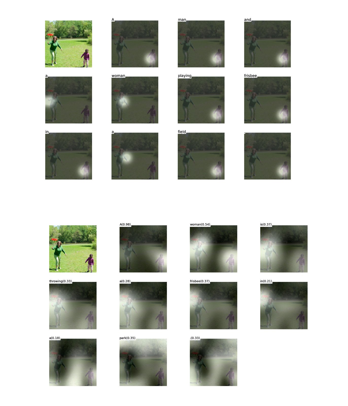
(a) A man and a woman playing frisbee in a field.
(b) A woman is throwing a frisbee in a park.
Figure 6:
(a)一男一女在田野里玩飞盘。
(b)一位女士在公园里扔飞盘。
图 6:
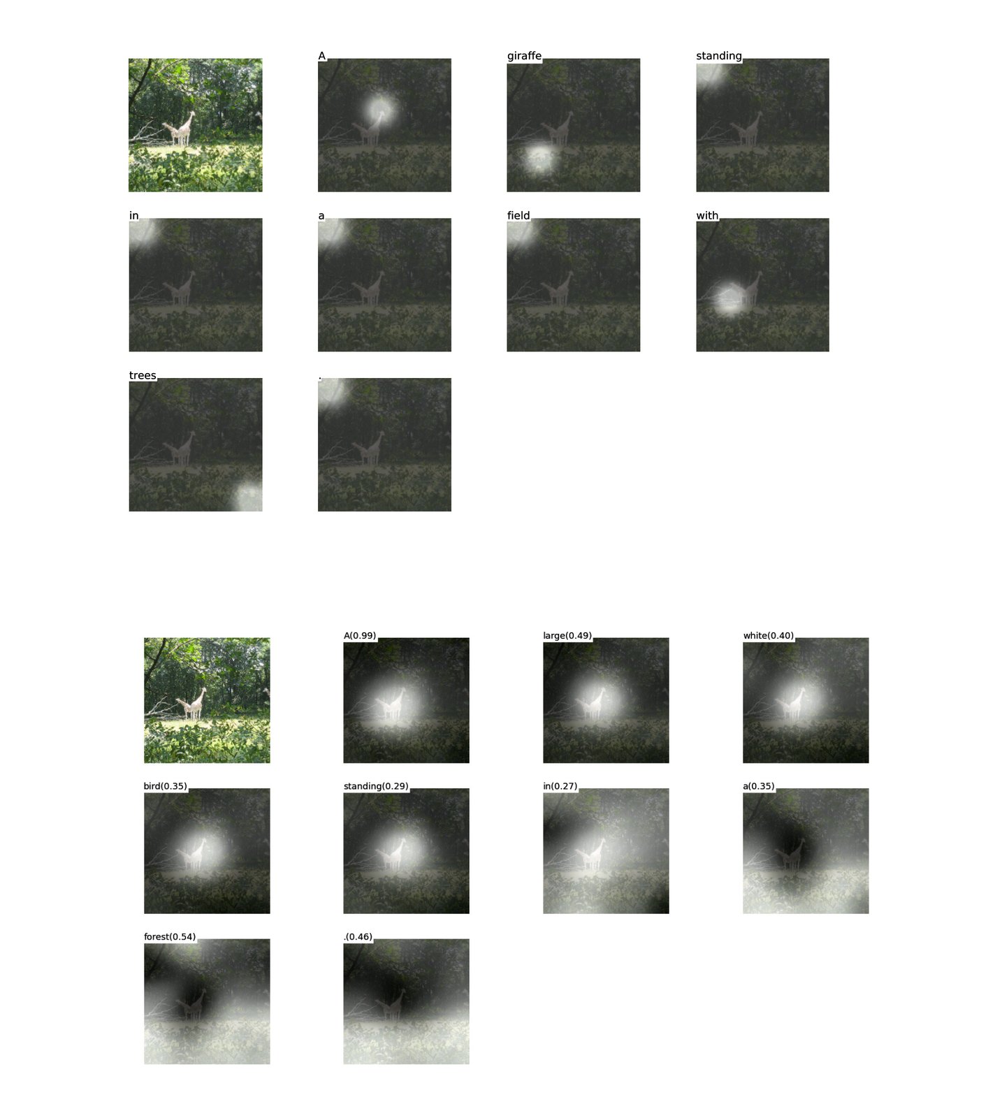
(a) A giraffe standing in the field with trees.
(b) A large white bird standing in a forest.
Figure 7:
(a)一只长颈鹿站在有树的田野里。
(b)一只大白鸟站在森林里。
图 7:
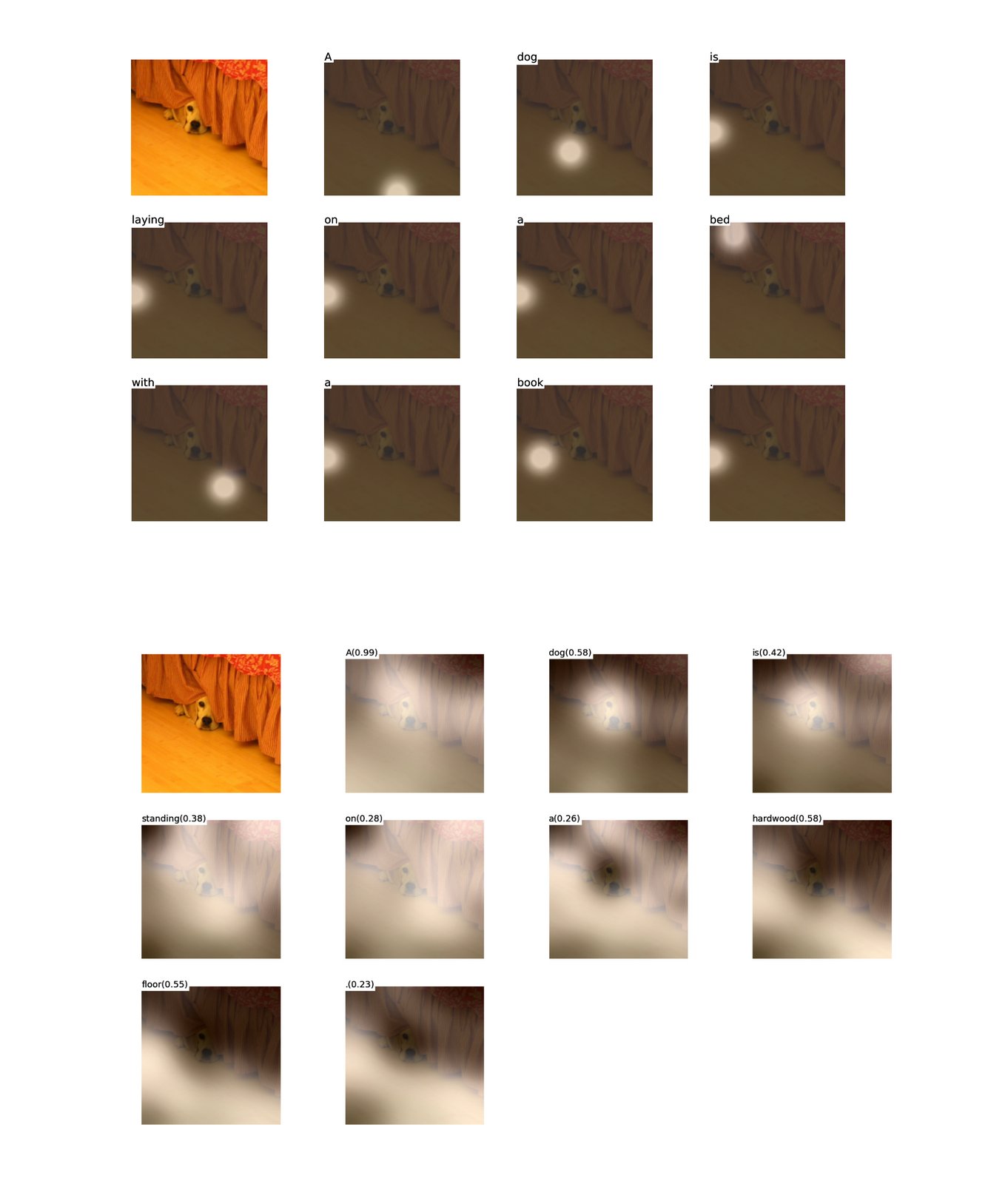
(a) A dog is laying on a bed with a book.
(b) A dog is standing on a hardwood floor.
Figure 8:
(a)一只狗躺在床上,旁边有一本书。
(b)一只狗站在硬木地板上。
图 8:
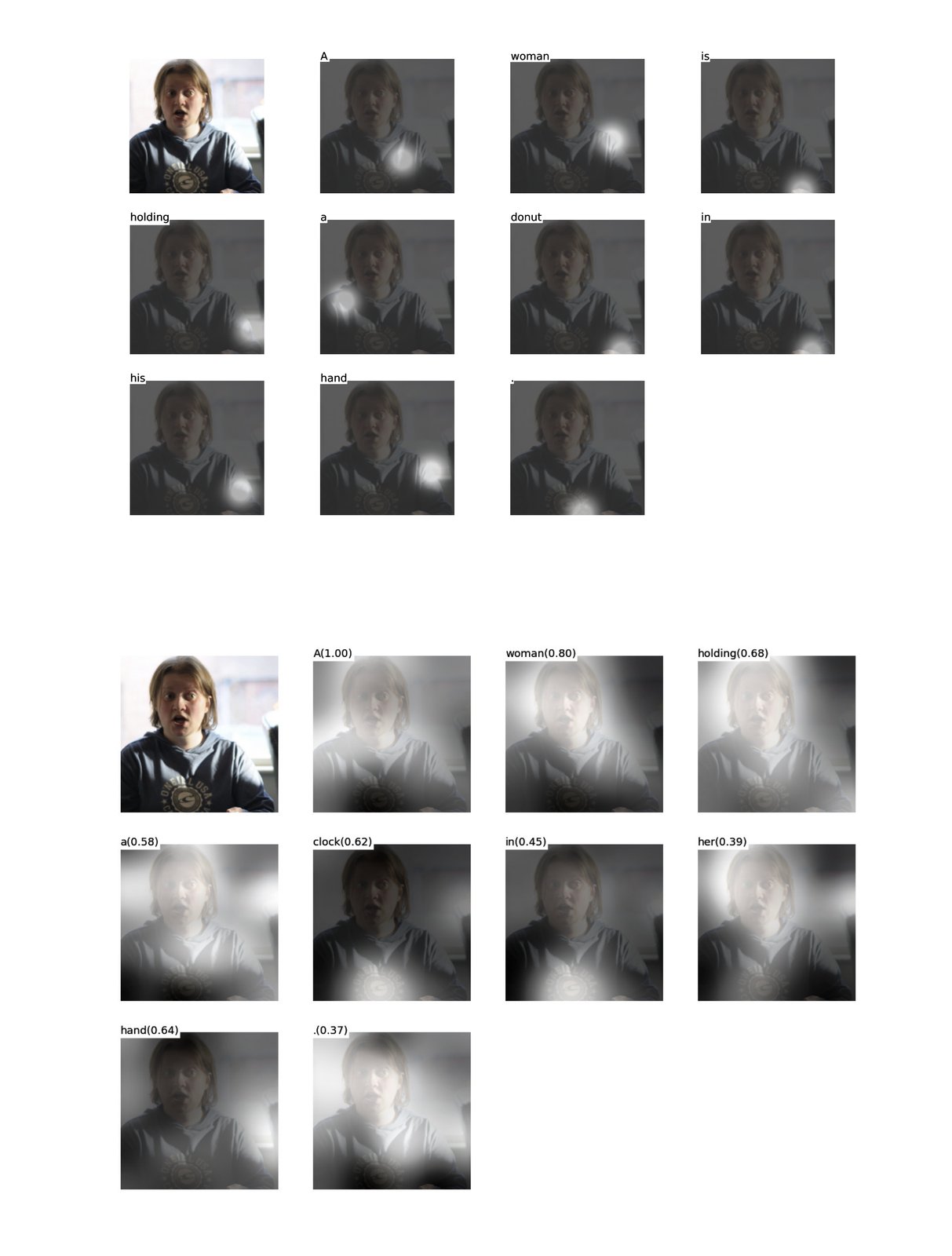
(a) A woman is holding a donut in his hand.
(b) A woman holding a clock in her hand.
Figure 9:
(a)一位女士手里拿着甜甜圈。
(b)一位女士手里拿着一只钟。
图 9:
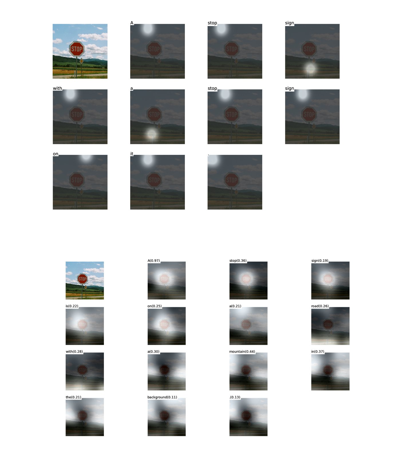
(a) A stop sign with a stop sign on it.
(b) A stop sign is on a road with a mountain in the background.
Figure 10:
(a)一块上面又有停车标志的停车标志。
(b)路边有一块停车标志,背景是山。
图 10:
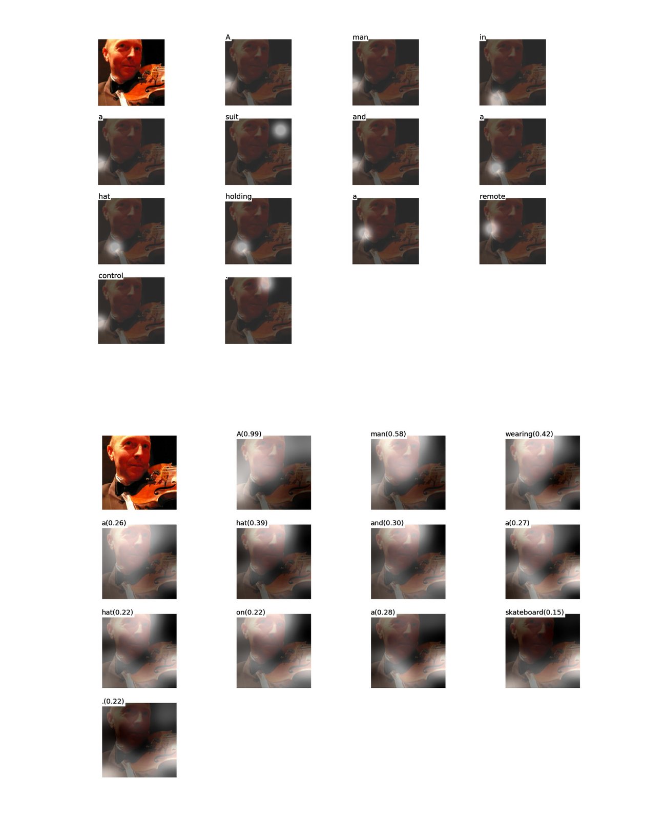
(a) A man in a suit and a hat holding a remote control.
(b) A man wearing a hat and a hat on a skateboard.
Figure 11:
(a)一位穿西装戴帽子的男士拿着遥控器。
(b)一位戴帽子的男士在滑板上。
图 11:
(a) A little girl sitting on a couch with a teddy bear.
(b) A little girl sitting on a bed with a teddy bear.
(a)一个小女孩坐在沙发上,抱着泰迪熊。
(b)一个小女孩坐在床上,抱着泰迪熊。
(a) A man is standing on a beach with a surfboard.
(b) A person is standing on a beach with a surfboard.
(a)一位男士拿着冲浪板站在海滩上。
(b)一个人拿着冲浪板站在海滩上。
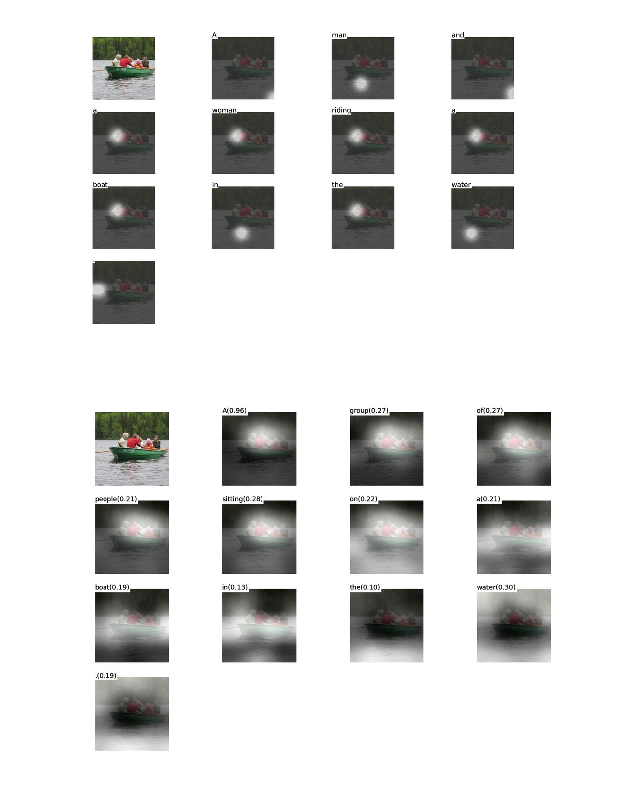
(a) A man and a woman riding a boat in the water.
(b) A group of people sitting on a boat in the water.
Figure 12:
(a)一男一女在水上乘船。
(b)一群人坐在水上的船上。
图 12:
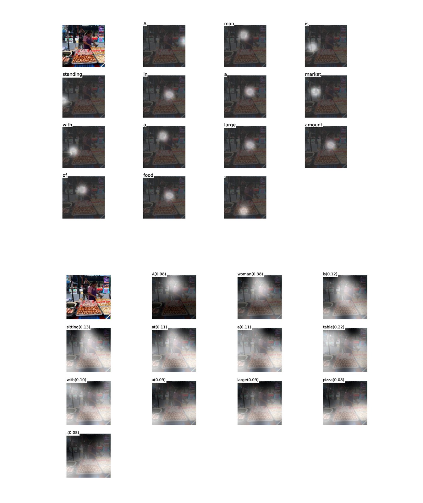
(a) A man is standing in a market with a large amount of food.
(b) A woman is sitting at a table with a large pizza.
Figure 13:
(a)一位男士站在摆满食物的市场里。
(b)一位女士坐在桌边,面前是一大块披萨。
图 13:
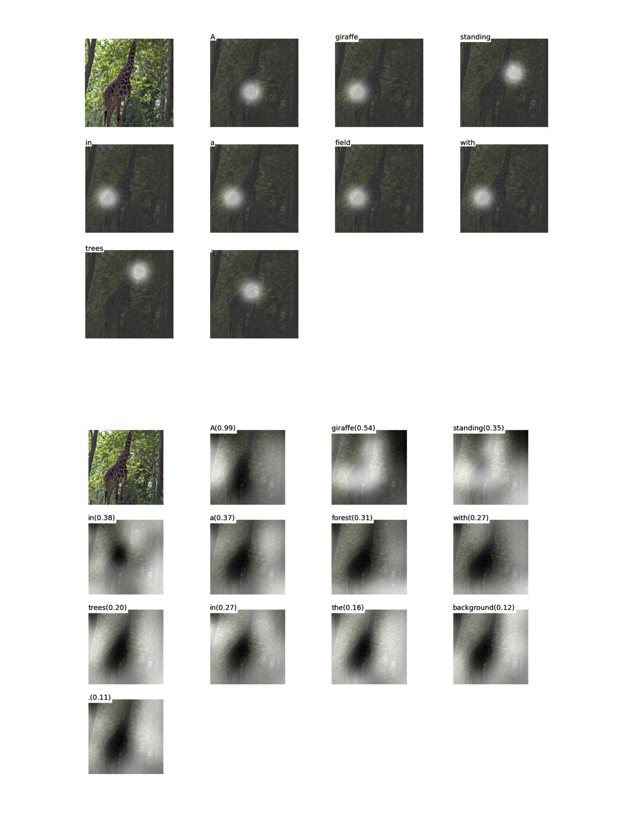
(a) A giraffe standing in a field with trees.
(b) A giraffe standing in a forest with trees in the background.
Figure 14:
(a)一只长颈鹿站在有树的田野里。
(b)一只长颈鹿站在森林里,背景有树。
图 14:
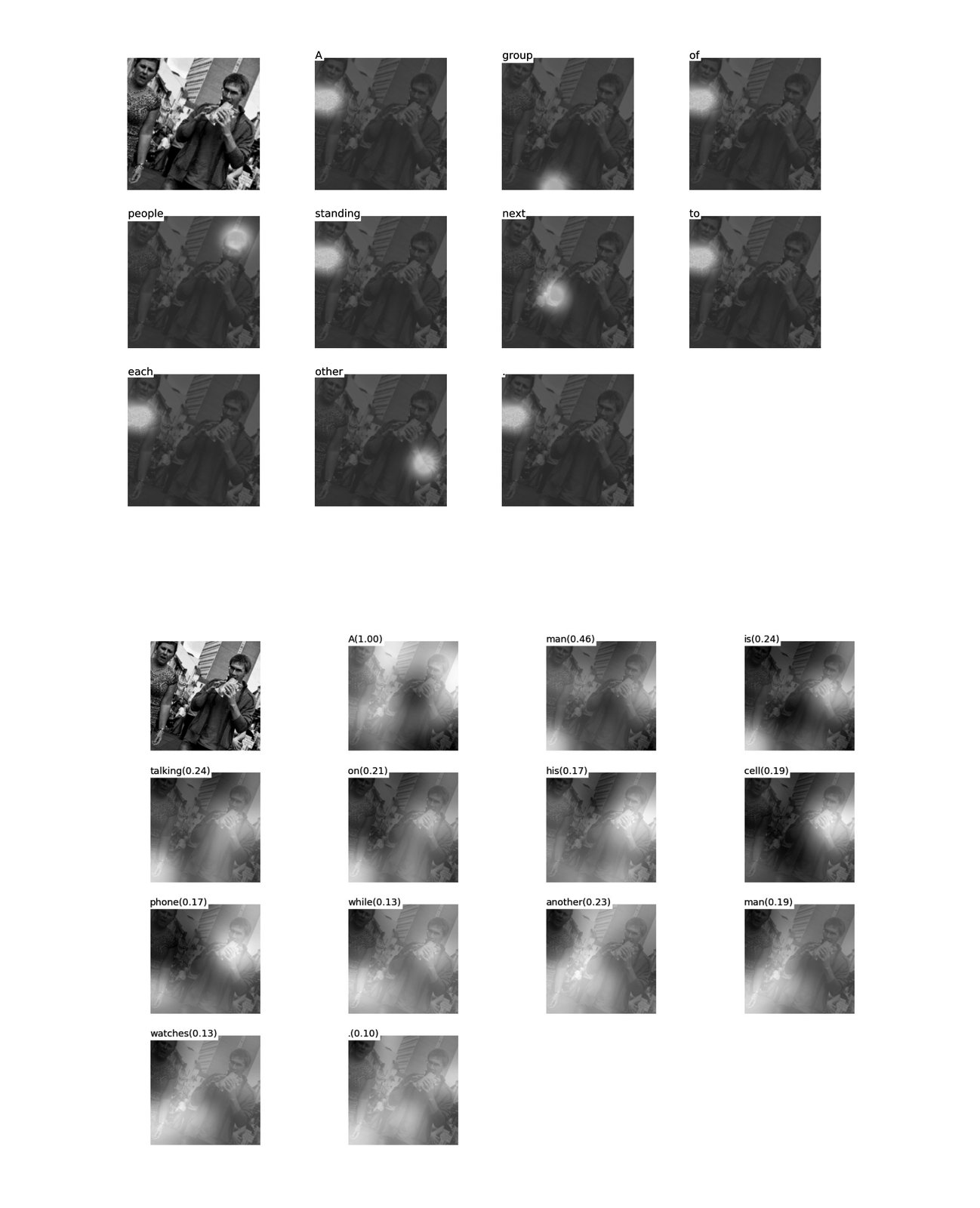
(a) A group of people standing next to each other.
(b) A man is talking on his cell phone while another man watches.
Figure 15:
(a)一群人并排站着。
(b)一位男士在打电话,另一位男士在看。
图 15: