Show and Tell: A Neural Image Caption Generator

Show and Tell：一种神经图像描述生成器

Oriol Vinyals
Google
vinyals@google.com
Alexander Toshev
Google
toshev@google.com
Samy Bengio
Google
bengio@google.com
Dumitru Erhan
Google
dumitru@google.com

Abstract

摘要

Automatically describing the content of an image is a fundamental problem in artificial intelligence that connects computer vision and natural language processing. In this paper, we present a generative model based on a deep recurrent architecture that combines recent advances in computer vision and machine translation and that can be used to generate natural sentences describing an image.

自动写出一张图的内容，是人工智能里把计算机视觉和自然语言处理连在一起的一个基本问题。本文给出一个基于深度循环结构的生成模型：它把计算机视觉和机器翻译里较新的进展合在一起，用来生成描述图像的自然语句。

The model is trained to maximize the likelihood of the target description sentence given the training image. Experiments on several datasets show the accuracy of the model and the fluency of the language it learns solely from image descriptions. Our model is often quite accurate, which we verify both qualitatively and quantitatively. For instance, while the current state-of-the-art BLEU-1 score (the higher the better) on the Pascal dataset is 25, our approach yields 59, to be compared to human performance around 69. We also show BLEU-1 score improvements on Flickr30k, from 56 to 66, and on SBU, from 19 to 28. Lastly, on the newly released COCO dataset, we achieve a BLEU-4 of 27.7, which is the current state-of-the-art.

训练目标是：在给定训练图像时，最大化目标描述句的似然。在多套数据上的实验表明，这个模型的准确性，以及它仅仅从图像描述里学到的语言通顺程度。我们的模型常常相当准确，这一点我们从定性和定量两方面都做了核验。例如，Pascal 上当时最好的 BLEU-1（越高越好）是 25，我们的方法得到 59，人工水平大约是 69。我们也报告了 Flickr30k 上 BLEU-1 从 56 提到 66，以及 SBU 上从 19 提到 28。最后，在新发布的 COCO 上，我们得到 BLEU-4 为 27.7，这是当时最好的结果。

1. Introduction

1. 引言

Being able to automatically describe the content of an image using properly formed English sentences is a very challenging task, but it could have great impact, for instance by helping visually impaired people better understand the content of images on the web. This task is significantly harder, for example, than the well-studied image classification or object recognition tasks, which have been a main focus in the computer vision community [27]. Indeed, a description must capture not only the objects contained in an image, but it also must express how these objects relate to each other as well as their attributes and the activities they are involved in. Moreover, the above semantic knowledge has to be expressed in a natural language like English, which means that a language model is needed in addition to visual understanding.

用语法正确的英文句子自动描述一张图的内容，是一项很有难度的任务，但影响可能很大，比如帮助视障人士更好地理解网上的图像内容。它比方说比已经研究得很充分的图像分类或物体识别要难得多，后两者一直是计算机视觉社区的主要关注点 [27]。描述不仅要抓住图中的物体，还要说出这些物体彼此如何关联、它们有什么属性、以及它们在做哪些活动。而且这些语义还要用英语这样的自然语言写出来，所以除了视觉理解，还需要一个语言模型。

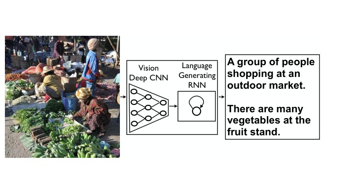
Figure 1. NIC, our model, is based end-to-end on a neural network consisting of a vision CNN followed by a language generating RNN. It generates complete sentences in natural language from an input image, as shown on the example above.

图 1. 我们的模型 NIC 是端到端的神经网络：前面是视觉 CNN，后面是生成语言的 RNN。它从输入图像生成完整的自然语言句子，如上例所示。

Most previous attempts have proposed to stitch together existing solutions of the above sub-problems, in order to go from an image to its description [6, 16]. In contrast, we would like to present in this work a single joint model that takes an image I as input, and is trained to maximize the likelihood p(S|I) of producing a target sequence of words S = {S1, S2, . . .} where each word St comes from a given dictionary, that describes the image adequately.

此前多数尝试是把上述子问题的现成解法拼接起来，从而从图像走到描述 [6, 16]。与此不同，我们希望在本文给出一个单一的联合模型：输入是图像 I，训练目标是最大化生成目标词序列 S = {S1, S2, …} 的似然 p(S|I)，其中每个词 St 来自给定词典，并且能够恰当地描述这张图。

The main inspiration of our work comes from recent advances in machine translation, where the task is to transform a sentence S written in a source language, into its translation T in the target language, by maximizing p(T|S). For many years, machine translation was also achieved by a series of separate tasks (translating words individually, aligning words, reordering, etc), but recent work has shown that translation can be done in a much simpler way using Recurrent Neural Networks (RNNs) [3, 2, 30] and still reach state-of-the-art performance. An “encoder” RNN reads the source sentence and transforms it into a rich fixed-length vector representation, which in turn in used as the initial hidden state of a “decoder” RNN that generates the target sentence.

我们工作的主要启发来自机器翻译的近期进展：任务是把源语言中的句子 S 变成目标语言中的译文 T，通过最大化 p(T|S) 来完成。多年来，机器翻译也是拆成一串分开的子任务（逐词翻译、对齐、调序等），但近来的工作表明，用循环神经网络（RNN）[3, 2, 30] 可以更简单地做翻译，并且仍然能达到当时最好的水平。一个「编码器」RNN 读入源句，把它变成丰富的定长向量表示，再把这个表示用作「解码器」RNN 的初始隐状态，由后者生成目标句。

Here, we propose to follow this elegant recipe, replacing the encoder RNN by a deep convolution neural network (CNN). Over the last few years it has been convincingly shown that CNNs can produce a rich representation of the input image by embedding it to a fixed-length vector, such that this representation can be used for a variety of vision tasks [28]. Hence, it is natural to use a CNN as an image “encoder”, by first pre-training it for an image classification task and using the last hidden layer as an input to the RNN decoder that generates sentences (see Fig. 1). We call this model the Neural Image Caption, or NIC.

这里我们沿用这一简洁做法，只是把编码器 RNN 换成深度卷积神经网络（CNN）。过去几年已经较有说服力地表明，CNN 可以把输入图像嵌入成定长向量，得到丰富的表示，并用于多种视觉任务 [28]。因此，很自然地把 CNN 当作图像「编码器」：先在图像分类任务上预训练，再用最后一层隐表示作为生成句子的 RNN 解码器的输入（见图 1）。我们把这个模型叫做 Neural Image Caption，简称 NIC。

Our contributions are as follows. First, we present an end-to-end system for the problem. It is a neural net which is fully trainable using stochastic gradient descent. Second, our model combines state-of-art sub-networks for vision and language models. These can be pre-trained on larger corpora and thus can take advantage of additional data. Finally, it yields significantly better performance compared to state-of-the-art approaches; for instance, on the Pascal dataset, NIC yielded a BLEU score of 59, to be compared to the current state-of-the-art of 25, while human performance reaches 69. On Flickr30k, we improve from 56 to 66, and on SBU, from 19 to 28.

我们的贡献如下。第一，我们为这个问题给出一个端到端系统：这是一个完全可以用随机梯度下降训练的神经网络。第二，我们的模型把视觉和语言模型里当时先进的子网络组合起来。它们可以在更大的语料上预训练，从而利用额外数据。最后，它的表现明显好于当时最好的方法；例如在 Pascal 上，NIC 的 BLEU 为 59，当时最好结果是 25，人工水平达到 69。在 Flickr30k 上，我们从 56 提到 66；在 SBU 上，从 19 提到 28。

2. Related Work

2. 相关工作

The problem of generating natural language descriptions from visual data has long been studied in computer vision, but mainly for video [7, 32]. This has led to complex systems composed of visual primitive recognizers combined with a structured formal language, e.g. And-Or Graphs or logic systems, which are further converted to natural language via rule-based systems. Such systems are heavily hand-designed, relatively brittle and have been demonstrated only on limited domains, e.g. traffic scenes or sports.

从视觉数据生成自然语言描述，在计算机视觉里已经研究了很久，但主要是针对视频 [7, 32]。由此出现的系统往往很复杂：先识别视觉基元，再与结构化的形式语言（例如与或图或逻辑系统）结合，最后用基于规则的系统转成自然语言。这类系统手工设计的成分很重，也比较脆弱，而且只在有限领域里演示过，例如交通场景或体育。

The problem of still image description with natural text has gained interest more recently. Leveraging recent advances in recognition of objects, their attributes and locations, allows us to drive natural language generation systems, though these are limited in their expressivity. Farhadi et al. [6] use detections to infer a triplet of scene elements which is converted to text using templates. Similarly, Li et al. [19] start off with detections and piece together a final description using phrases containing detected objects and relationships. A more complex graph of detections beyond triplets is used by Kulkani et al. [16], but with template-based text generation. More powerful language models based on language parsing have been used as well [23, 1, 17, 18, 5]. The above approaches have been able to describe images “in the wild”, but they are heavily hand-designed and rigid when it comes to text generation.

用自然语言描述静态图像，是更近才受到关注的问题。借助物体、属性与位置识别的进展，可以驱动自然语言生成系统，不过这些系统的表达能力仍然有限。Farhadi 等人 [6] 用检测结果推断场景要素三元组，再用模板转成文本。类似地，Li 等人 [19] 也从检测出发，用包含被检物体和关系的短语拼出最终描述。Kulkani 等人 [16] 用了比三元组更复杂的检测图，但文本生成仍是基于模板。也有工作使用基于句法分析、能力更强的语言模型 [23, 1, 17, 18, 5]。上述方法已经能描述「野外」图像，但手工设计很重，生成文本时也比较死板。

A large body of work has addressed the problem of ranking descriptions for a given image [11, 8, 24]. Such approaches are based on the idea of co-embedding of images and text in the same vector space. For an image query, descriptions are retrieved which lie close to the image in the embedding space. Most closely, neural networks are used to co-embed images and sentences together [29] or even image crops and subsentences [13] but do not attempt to generate novel descriptions. In general, the above approaches cannot describe previously unseen compositions of objects, even though the individual objects might have been observed in the training data. Moreover, they avoid addressing the problem of evaluating how good a generated description is.

还有大量工作讨论的是：给定一张图，如何给已有描述排序 [11, 8, 24]。这类方法的想法是把图像和文本共同嵌入同一个向量空间。对于图像查询，就取嵌入空间里离这张图近的描述。最接近的做法是用神经网络把图像和句子一起嵌入 [29]，甚至把图像裁块和子句一起嵌入 [13]，但并不试图生成新的描述。总的来说，上述方法无法描述此前没见过的物体组合，即便单个物体在训练数据里出现过。此外，它们也回避了如何评价生成描述好坏这一问题。

In this work we combine deep convolutional nets for image classification [12] with recurrent networks for sequence modeling [10], to create a single network that generates descriptions of images. The RNN is trained in the context of this single “end-to-end” network. The model is inspired by recent successes of sequence generation in machine translation [3, 2, 30], with the difference that instead of starting with a sentence, we provide an image processed by a convolutional net. The closest works are by Kiros et al. [15] who use a neural net, but a feedforward one, to predict the next word given the image and previous words. A recent work by Mao et al. [21] uses a recurrent NN for the same prediction task. This is very similar to the present proposal but there are a number of important differences: we use a more powerful RNN model, and provide the visual input to the RNN model directly, which makes it possible for the RNN to keep track of the objects that have been explained by the text. As a result of these seemingly insignificant differences, our system achieves substantially better results on the established benchmarks. Lastly, Kiros et al. [14] propose to construct a joint multimodal embedding space by using a powerful computer vision model and an LSTM that encodes text. In contrast to our approach, they use two separate pathways (one for images, one for text) to define a joint embedding, and, even though they can generate text, their approach is highly tuned for ranking.

本文把用于图像分类的深度卷积网络 [12] 和用于序列建模的循环网络 [10] 结合起来，做成一个生成图像描述的单一网络。RNN 是在这个单一的「端到端」网络里训练的。模型的启发来自机器翻译中序列生成的近期成功 [3, 2, 30]，不同之处在于：我们不是从句子出发，而是提供一张经过卷积网络处理的图像。最接近的工作是 Kiros 等人 [15]，他们也用神经网络根据图像和已有词预测下一个词，但用的是前馈网络。Mao 等人 [21] 近期用循环神经网络做同一预测任务。这和本文的方案很像，但有几处重要不同：我们用了更强的 RNN 模型，并且把视觉输入直接送给 RNN，使 RNN 能够跟踪文本已经说明过哪些物体。这些看起来不大的差别，却让我们的系统在已有基准上明显更好。最后，Kiros 等人 [14] 提出用强大的视觉模型和编码文本的 LSTM 构造联合多模态嵌入空间。与我们不同，他们用两条分开的通路（一条图像、一条文本）来定义联合嵌入；虽然也能生成文本，但其方法主要是为排序任务调的。

3. Model

3. 模型

In this paper, we propose a neural and probabilistic framework to generate descriptions from images. Recent advances in statistical machine translation have shown that, given a powerful sequence model, it is possible to achieve state-of-the-art results by directly maximizing the probability of the correct translation given an input sentence in an “end-to-end” fashion – both for training and inference. These models make use of a recurrent neural network which encodes the variable length input into a fixed dimensional vector, and uses this representation to “decode” it to the desired output sentence. Thus, it is natural to use the same approach where, given an image (instead of an input sentence in the source language), one applies the same principle of “translating” it into its description.

本文提出一个神经、概率的框架，用来从图像生成描述。统计机器翻译的近期进展表明：只要有足够强的序列模型，就可以用「端到端」的方式直接最大化正确译文在给定输入句时的概率，训练和推断都是如此，并达到当时最好结果。这类模型用循环神经网络把可变长度的输入编成固定维向量，再用这个表示「解码」出目标输出句。因此，很自然地把同样的思路用到图像上：给定一张图（而不是源语言中的输入句），用同样的原则把它「翻译」成描述。

Thus, we propose to directly maximize the probability of the correct description given the image by using the following formulation:

于是，我们提出直接最大化正确描述在给定图像时的概率，采用如下写法：

θ⋆ = arg max_θ Σ_{(I,S)} log p(S|I; θ) (1)

where θ are the parameters of our model, I is an image, and S its correct transcription. Since S represents any sentence, its length is unbounded. Thus, it is common to apply the chain rule to model the joint probability over S0, . . . , SN, where N is the length of this particular example as

其中 θ 是模型参数，I 是图像，S 是它的正确转写。由于 S 可以是任意句子，长度没有上界。因此通常用链式法则来建模 S0, …, SN 上的联合概率，其中 N 是这个样本的长度：

log p(S|I) = Σ_{t=0}^{N} log p(S_t | I, S_0, . . . , S_{t−1}) (2)

where we dropped the dependency on θ for convenience. At training time, (S, I) is a training example pair, and we optimize the sum of the log probabilities as described in (2) over the whole training set using stochastic gradient descent (further training details are given in Section 4).

为方便起见，这里去掉了对 θ 的依赖。训练时，(S, I) 是一对训练样本，我们在整个训练集上用随机梯度下降优化 (2) 中的对数概率之和（更多训练细节见第 4 节）。

It is natural to model p(S_t|I, S_0, . . . , S_{t−1}) with a Recurrent Neural Network (RNN), where the variable number of words we condition upon up to t − 1 is expressed by a fixed length hidden state or memory h_t. This memory is updated after seeing a new input x_t by using a non-linear function f:

很自然地用循环神经网络（RNN）来建模 p(S_t|I, S_0, …, S_{t−1})：到 t−1 为止所条件于的可变数量的词，用一个定长隐状态或记忆 h_t 来表示。看到新输入 x_t 之后，用非线性函数 f 更新这个记忆：

h_{t+1} = f(h_t, x_t) . (3)

To make the above RNN more concrete two crucial design choices are to be made: what is the exact form of f and how are the images and words fed as inputs x_t. For f we use a Long-Short Term Memory (LSTM) net, which has shown state-of-the art performance on sequence tasks such as translation. This model is outlined in the next section.

要把上述 RNN 落成具体模型，有两个关键设计选择：f 的具体形式是什么，以及图像和词怎样作为输入 x_t 送进去。对 f，我们采用长短期记忆网络（LSTM），它在翻译等序列任务上已表现出当时一流的水平。下一节概述这一模型。

For the representation of images, we use a Convolutional Neural Network (CNN). They have been widely used and studied for image tasks, and are currently state-of-the art for object recognition and detection. Our particular choice of CNN uses a novel approach to batch normalization and yields the current best performance on the ILSVRC 2014 classification competition [12]. Furthermore, they have been shown to generalize to other tasks such as scene classification by means of transfer learning [4]. The words are represented with an embedding model.

图像表示我们采用卷积神经网络（CNN）。它们在图像任务上已被广泛使用和研究，并且在物体识别和检测上是当时最好的一类方法。我们选用的 CNN 采用了一种新的批归一化做法，并在 ILSVRC 2014 分类竞赛上取得了当时最好的成绩 [12]。此外，借助迁移学习，它们也被表明可以推广到场景分类等其他任务 [4]。词则用嵌入模型来表示。

3.1. LSTM-based Sentence Generator

3.1. 基于 LSTM 的句子生成器

The choice of f in (3) is governed by its ability to deal with vanishing and exploding gradients [10], the most common challenge in designing and training RNNs. To address this challenge, a particular form of recurrent nets, called LSTM, was introduced [10] and applied with great success to translation [3, 30] and sequence generation [9].

(3) 式中 f 的选择，取决于它处理梯度消失和爆炸的能力 [10]，这是设计和训练 RNN 时最常见的困难。为应对这一困难，人们提出了名为 LSTM 的一类循环网络 [10]，并在翻译 [3, 30] 和序列生成 [9] 上取得了很大成功。

The core of the LSTM model is a memory cell c encoding knowledge at every time step of what inputs have been observed up to this step (see Figure 2). The behavior of the cell is controlled by “gates” – layers which are applied multiplicatively and thus can either keep a value from the gated layer if the gate is 1 or zero this value if the gate is 0. In particular, three gates are being used which control whether to forget the current cell value (forget gate f), if it should read its input (input gate i) and whether to output the new cell value (output gate o). The definition of the gates and cell update and output are as follows:

LSTM 模型的核心是记忆单元 c，它在每个时间步编码到这一步为止已经观察到哪些输入（见图 2）。单元的行为由「门」控制——这些层以相乘的方式作用，因此门为 1 时保留被控层的值，门为 0 时把该值置零。具体用了三个门：是否忘记当前单元值（遗忘门 f）、是否读入输入（输入门 i），以及是否输出新的单元值（输出门 o）。各门以及单元更新与输出的定义如下：

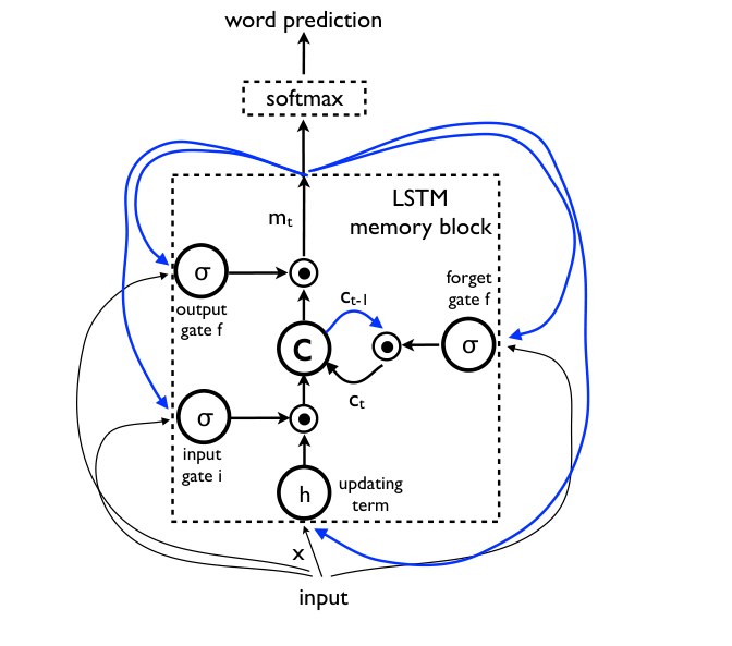
Figure 2. LSTM: the memory block contains a cell c which is controlled by three gates. In blue we show the recurrent connections – the output m at time t − 1 is fed back to the memory at time t via the three gates; the cell value is fed back via the forget gate; the predicted word at time t − 1 is fed back in addition to the memory output m at time t into the Softmax for word prediction.

图 2. LSTM：记忆块里有一个由三个门控制的单元 c。蓝色表示循环连接——时刻 t−1 的输出 m 经过三个门送回时刻 t 的记忆；单元值经遗忘门送回；时刻 t−1 的预测词，连同时刻 t 的记忆输出 m，一起送入 Softmax 做词预测。

i_t = σ(W_{ix} x_t + W_{im} m_{t−1}) (4)
f_t = σ(W_{fx} x_t + W_{fm} m_{t−1}) (5)
o_t = σ(W_{ox} x_t + W_{om} m_{t−1}) (6)
c_t = f_t ⊙ c_{t−1} + i_t ⊙ h(W_{cx} x_t + W_{cm} m_{t−1}) (7)
m_t = o_t ⊙ c_t (8)
p_{t+1} = Softmax(m_t) (9)

where ⊙ represents the product with a gate value, and the various W matrices are trained parameters. Such multiplicative gates make it possible to train the LSTM robustly as these gates deal well with exploding and vanishing gradients [10]. The nonlinearities are sigmoid σ(·) and hyperbolic tangent h(·). The last equation m_t is what is used to feed to a Softmax, which will produce a probability distribution p_t over all words.

其中 ⊙ 表示与门值相乘，各个 W 矩阵是待训练的参数。这种相乘的门使 LSTM 能够稳健地训练，因为它们能较好地应对梯度爆炸和消失 [10]。非线性是 sigmoid σ(·) 和双曲正切 h(·)。最后一式的 m_t 被送入 Softmax，得到在全部词上的概率分布 p_t。

Training

训练

The LSTM model is trained to predict each word of the sentence after it has seen the image as well as all preceding words as defined by p(S_t|I, S_0, . . . , S_{t−1}). For this purpose, it is instructive to think of the LSTM in unrolled form – a copy of the LSTM memory is created for the image and each sentence word such that all LSTMs share the same parameters and the output m_{t−1} of the LSTM at time t − 1 is fed to the LSTM at time t (see Figure 3). All recurrent connections are transformed to feed-forward connections in the unrolled version. In more detail, if we denote by I the input image and by S = (S_0, . . . , S_N) a true sentence describing this image, the unrolling procedure reads:

LSTM 的训练目标是：在已经看到图像以及前面所有词之后，按 p(S_t|I, S_0, …, S_{t−1}) 预测句子里的每一个词。为此，把 LSTM 想成展开形式会更清楚——为图像和句子中的每个词各放一份 LSTM 记忆的副本，所有 LSTM 共享同一套参数，并且时刻 t−1 的输出 m_{t−1} 送到时刻 t 的 LSTM（见图 3）。在展开版本里，所有循环连接都变成了前馈连接。更具体地，记 I 为输入图像，S = (S_0, …, S_N) 为描述该图的正确句子，展开过程可以写成：

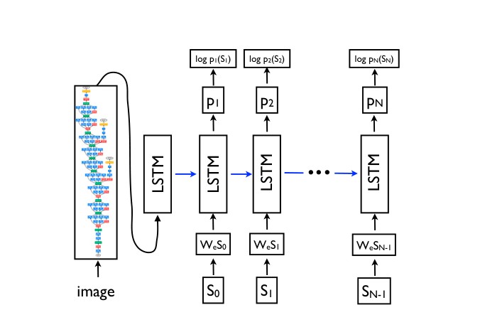
Figure 3. LSTM model combined with a CNN image embedder (as defined in [12]) and word embeddings. The unrolled connections between the LSTM memories are in blue and they correspond to the recurrent connections in Figure 2. All LSTMs share the same parameters.

图 3. LSTM 模型与 CNN 图像嵌入器（定义见 [12]）以及词嵌入结合在一起。LSTM 记忆之间展开后的连接用蓝色画出，它们对应图 2 中的循环连接。所有 LSTM 共享同一套参数。

x_{−1} = CNN(I) (10)
x_t = W_e S_t, t ∈ {0 . . . N − 1} (11)
p_{t+1} = LSTM(x_t), t ∈ {0 . . . N − 1} (12)

where we represent each word as a one-hot vector S_t of dimension equal to the size of the dictionary. Note that we denote by S_0 a special start word and by S_N a special stop word which designates the start and end of the sentence. In particular by emitting the stop word the LSTM signals that a complete sentence has been generated. Both the image and the words are mapped to the same space, the image by using a vision CNN, the words by using word embedding W_e. The image I is only input once, at t = −1, to inform the LSTM about the image contents. We empirically verified that feeding the image at each time step as an extra input yields inferior results, as the network can explicitly exploit noise in the image and overfits more easily.

其中每个词表示成维数等于词典大小的 one-hot 向量 S_t。我们用 S_0 表示一个特殊的起始词，用 S_N 表示一个特殊的终止词，用来标记句子的开头和结尾。尤其是，LSTM 一旦放出终止词，就表示已经生成了完整句子。图像和词被映射到同一个空间：图像通过视觉 CNN，词通过词嵌入 W_e。图像 I 只在 t = −1 时输入一次，用来把图像内容告诉 LSTM。我们通过实验核验过：如果在每个时间步都把图像当作额外输入送进去，效果反而更差，因为网络可以显式地利用图像里的噪声，也更容易过拟合。

Our loss is the sum of the negative log likelihood of the correct word at each step as follows:

我们的损失是每一步正确词的负对数似然之和，如下：

L(I, S) = − Σ_{t=1}^{N} log p_t(S_t) . (13)

The above loss is minimized w.r.t. all the parameters of the LSTM, the top layer of the image embedder CNN and word embeddings W_e.

上述损失对 LSTM 的全部参数、图像嵌入 CNN 的顶层以及词嵌入 W_e 做最小化。

Inference

推断

There are multiple approaches that can be used to generate a sentence given an image, with NIC. The first one is Sampling where we just sample the first word according to p_1, then provide the corresponding embedding as input and sample p_2, continuing like this until we sample the special end-of-sentence token or some maximum length. The second one is BeamSearch: iteratively consider the set of the k best sentences up to time t as candidates to generate sentences of size t + 1, and keep only the resulting best k of them. This better approximates S = arg max_{S'} p(S'|I). We used the BeamSearch approach in the following experiments, with a beam of size 20. Using a beam size of 1 (i.e., greedy search) did degrade our results by 2 BLEU points on average.

给定一张图，NIC 可以用多种方式生成句子。第一种是采样：按 p_1 采出第一个词，再把对应嵌入作为输入去采 p_2，如此继续，直到采到特殊的句末标记，或达到某个最大长度。第二种是束搜索：迭代地把到时刻 t 为止最好的 k 个句子当作候选，用来生成长度为 t+1 的句子，再只保留其中最好的 k 个。这样能更好地逼近 S = arg max_{S'} p(S'|I)。后面的实验里我们用束搜索，束宽为 20。把束宽设为 1（即贪心搜索）会使结果平均下降 2 个 BLEU 点。

4. Experiments

4. 实验

We performed an extensive set of experiments to assess the effectiveness of our model using several metrics, data sources, and model architectures, in order to compare to prior art.

我们做了一组较完整的实验，用多种指标、数据来源和模型结构来评估效果，以便与已有工作比较。

4.1. Evaluation Metrics

4.1. 评价指标

Although it is sometimes not clear whether a description should be deemed successful or not given an image, prior art has proposed several evaluation metrics. The most reliable (but time consuming) is to ask for raters to give a subjective score on the usefulness of each description given the image. In this paper, we used this to reinforce that some of the automatic metrics indeed correlate with this subjective score, following the guidelines proposed in [11], which asks the graders to evaluate each generated sentence with a scale from 1 to 4.

给定一张图，有时并不容易判断一条描述算不算成功，但已有工作提出了若干评价指标。最可靠（但也最费时）的是请评分人就每条描述对这张图的有用程度给出主观分数。本文用这一做法来进一步确认：某些自动指标的确与这种主观分数相关。我们遵循 [11] 提出的指南，请评分人按 1 到 4 分给每条生成句打分。

1 The raters are asked whether the image is described without any errors, described with minor errors, with a somewhat related description, or with an unrelated description, with a score of 4 being the best and 1 being the worst.

注 1：评分人需要判断图像是被毫无差错地描述、带有轻微错误地描述、描述只是有些相关，还是描述并不相关；4 分最好，1 分最差。

For this metric, we set up an Amazon Mechanical Turk experiment. Each image was rated by 2 workers. The typical level of agreement between workers is 65%. In case of disagreement we simply average the scores and record the average as the score. For variance analysis, we perform bootstrapping (re-sampling the results with replacement and computing means/standard deviation over the resampled results). Like [11] we report the fraction of scores which are larger or equal than a set of predefined thresholds.

为这一指标，我们在 Amazon Mechanical Turk 上做了实验。每张图由 2 名工作人员评分。工作人员之间的典型一致率是 65%。意见不一致时，我们直接把分数取平均，并把平均值记为该样本的分数。为分析方差，我们做自助法（有放回地重采样结果，再在重采样结果上计算均值和标准差）。与 [11] 一样，我们报告分数大于或等于一组预定阈值的比例。

The rest of the metrics can be computed automatically assuming one has access to groundtruth, i.e. human generated descriptions. The most commonly used metric so far in the image description literature has been the BLEU score [25], which is a form of precision of word n-grams between generated and reference sentences. Even though this metric has some obvious drawbacks, it has been shown to correlate well with human evaluations. In this work, we corroborate this as well, as we show in Section 4.3. An extensive evaluation protocol, as well as the generated outputs of our system, can be found at http://nic.droppages.com/.

其余指标在有人工生成的参考描述（即真值）时可以自动计算。图像描述文献里迄今最常用的是 BLEU 分数 [25]，它衡量的是生成句和参考句之间词 n 元组的一种精度。尽管这一指标有一些明显缺点，但已被表明与人工评价相关性较好。本文在第 4.3 节也对此做了印证。更完整的评价协议以及本系统的生成结果，见 http://nic.droppages.com/。

2 In this literature, most previous work report BLEU-1, i.e., they only compute precision at the unigram level, whereas BLEU-n is a geometric average of precision over 1- to n-grams.

注 2：在这一文献里，此前多数工作报告的是 BLEU-1，也就是只计算一元文法上的精度；而 BLEU-n 是 1 到 n 元文法精度的几何平均。

Besides BLEU, one can use the perplexity of the model for a given transcription (which is closely related to our objective function in (1)). The perplexity is the geometric mean of the inverse probability for each predicted word. We used this metric to perform choices regarding model selection and hyperparameter tuning in our held-out set, but we do not report it since BLEU is always preferred.

除了 BLEU，还可以用模型对给定转写的困惑度（这与 (1) 中的目标函数密切相关）。困惑度是每个预测词的概率倒数的几何平均。我们用这一指标在留出集上做模型选择和超参数调节，但并不在文中报告，因为总是更倾向于报告 BLEU。

3 Even though it would be more desirable, optimizing for BLEU score yields a discrete optimization problem. In general, perplexity and BLEU scores are fairly correlated.

注 3：尽管直接优化 BLEU 会更理想，但这会变成离散优化问题。一般而言，困惑度与 BLEU 分数相当相关。

A much more detailed discussion regarding metrics can be found in [31], and research groups working on this topic have been reporting other metrics which are deemed more appropriate for evaluating caption. We report two such metrics – METEOR and Cider – hoping for much more discussion and research to arise regarding the choice of metric.

关于指标的更细致讨论见 [31]；做这一课题的研究组也在报告其他被认为更适合评价描述的指标。我们报告其中两种——METEOR 和 Cider——希望围绕指标选择出现更多讨论和研究。

Lastly, the current literature on image description has also been using the proxy task of ranking a set of available descriptions with respect to a given image (see for instance [14]). Doing so has the advantage that one can use known ranking metrics like recall@k. On the other hand, transforming the description generation task into a ranking task is unsatisfactory: as the complexity of images to describe grows, together with its dictionary, the number of possible sentences grows exponentially with the size of the dictionary, and the likelihood that a predefined sentence will fit a new image will go down unless the number of such sentences also grows exponentially, which is not realistic; not to mention the underlying computational complexity of evaluating efficiently such a large corpus of stored sentences for each image. The same argument has been used in speech recognition, where one has to produce the sentence corresponding to a given acoustic sequence; while early attempts concentrated on classification of isolated phonemes or words, state-of-the-art approaches for this task are now generative and can produce sentences from a large dictionary.

最后，当前图像描述文献也把「相对给定图像，对一组已有描述排序」当作替代任务（例如见 [14]）。这样做的好处是可以用 Recall@k 这类已知的排序指标。另一方面，把描述生成变成排序并不令人满意：随着要描述的图像变复杂、词典变大，可能的句子数目会随词典大小指数增长；除非预先存好的句子数目也指数增长（这并不现实），否则一条预先写好的句子能配上一张新图的可能性会下降；更不必说对每张图高效检索如此庞大的存句库所带来的计算复杂度。语音识别里也有过同样的论证：任务是为给定声学序列写出对应句子；早期尝试集中在孤立音素或词的分类上，而现在这一任务上最好的方法已经是生成式的，并能从很大的词典里产出句子。

Now that our models can generate descriptions of reasonable quality, and despite the ambiguities of evaluating an image description (where there could be multiple valid descriptions not in the groundtruth) we believe we should concentrate on evaluation metrics for the generation task rather than for ranking.

既然我们的模型已经能生成质量尚可的描述，尽管评价图像描述仍有含糊之处（可能有多条合理描述并不在真值里），我们认为应当把评价集中在生成任务本身，而不是排序。

4.2. Datasets

4.2. 数据集

For evaluation we use a number of datasets which consist of images and sentences in English describing these images. The statistics of the datasets are as follows:

评价时我们使用若干由图像和描述这些图像的英文句子组成的数据集。各数据集的规模如下：

Dataset name	size train	size valid.	size test
Pascal VOC 2008 [6]	–	–	1000
Flickr8k [26]	6000	1000	1000
Flickr30k [33]	28000	1000	1000
MSCOCO [20]	82783	40504	40775
SBU [24]	1M	–	–

数据集	训练集规模	验证集规模	测试集规模
Pascal VOC 2008 [6]	–	–	1000
Flickr8k [26]	6000	1000	1000
Flickr30k [33]	28000	1000	1000
MSCOCO [20]	82783	40504	40775
SBU [24]	1M	–	–

With the exception of SBU, each image has been annotated by labelers with 5 sentences that are relatively visual and unbiased. SBU consists of descriptions given by image owners when they uploaded them to Flickr. As such they are not guaranteed to be visual or unbiased and thus this dataset has more noise.

除 SBU 外，每张图都由标注者写了 5 句相对视觉化、也相对中性的句子。SBU 的描述来自图像所有者把照片上传到 Flickr 时写下的文字。因此它们并不保证是视觉化或中性的，这套数据噪声也更大。

The Pascal dataset is customary used for testing only after a system has been trained on different data such as any of the other four dataset. In the case of SBU, we hold out 1000 images for testing and train on the rest as used by [18]. Similarly, we reserve 4K random images from the MSCOCO validation set as test, called COCO-4k, and use it to report results in the following section.

Pascal 这套数据通常只作测试，系统要先在别的数据上训练，例如其余四套中的任何一套。对 SBU，我们留出 1000 张图作测试，其余用于训练，做法与 [18] 相同。类似地，我们从 MSCOCO 验证集中随机留出 4K 张图作为测试，称为 COCO-4k，并在下一节用它报告结果。

4.3. Results

4.3. 结果

Since our model is data driven and trained end-to-end, and given the abundance of datasets, we wanted to answer questions such as “how dataset size affects generalization”, “what kinds of transfer learning it would be able to achieve”, and “how it would deal with weakly labeled examples”. As a result, we performed experiments on five different datasets, explained in Section 4.2, which enabled us to understand our model in depth.

由于我们的模型是数据驱动、端到端训练的，而可用的数据集又不少，我们希望回答这样一些问题：「数据规模如何影响泛化」「能做成怎样的迁移学习」，以及「如何处理弱标注样本」。因此，我们在第 4.2 节说明的五套不同数据上做了实验，以便更深入地理解这个模型。

4.3.1 Training Details

4.3.1 训练细节

Many of the challenges that we faced when training our models had to do with overfitting. Indeed, purely supervised approaches require large amounts of data, but the datasets that are of high quality have less than 100000 images. The task of assigning a description is strictly harder than object classification and data driven approaches have only recently become dominant thanks to datasets as large as ImageNet (with ten times more data than the datasets we described in this paper, with the exception of SBU). As a result, we believe that, even with the results we obtained which are quite good, the advantage of our method versus most current human-engineered approaches will only increase in the next few years as training set sizes will grow.

训练这些模型时，我们遇到的许多困难都和过拟合有关。纯监督方法确实需要大量数据，但高质量数据集的图像数还不到 10 万。给图像配上描述，严格来说比物体分类更难；数据驱动方法最近才占主导，靠的是像 ImageNet 这样大规模的数据（除 SBU 外，其规模大约是本文所述数据集的十倍）。因此我们认为，即便我们已经得到了相当好的结果，随着训练集继续变大，我们的方法相对目前多数人工设计方法的优势，在接下来几年里只会进一步扩大。

Nonetheless, we explored several techniques to deal with overfitting. The most obvious way to not overfit is to initialize the weights of the CNN component of our system to a pretrained model (e.g., on ImageNet). We did this in all the experiments (similar to [8]), and it did help quite a lot in terms of generalization. Another set of weights that could be sensibly initialized are W_e, the word embeddings. We tried initializing them from a large news corpus [22], but no significant gains were observed, and we decided to just leave them uninitialized for simplicity. Lastly, we did some model level overfitting-avoiding techniques. We tried dropout [34] and ensembling models, as well as exploring the size (i.e., capacity) of the model by trading off number of hidden units versus depth. Dropout and ensembling gave a few BLEU points improvement, and that is what we report throughout the paper.

尽管如此，我们仍探索了若干应对过拟合的技术。最显而易见的办法，是把系统中 CNN 部分的权重初始化成预训练模型（例如在 ImageNet 上训好的）。所有实验都这样做了（与 [8] 类似），对泛化确实很有帮助。另一组可以合理初始化的权重是词嵌入 W_e。我们试过用大规模新闻语料 [22] 来初始化，但没有看到明显收益，为简单起见就让它们保持未初始化。最后，我们还做了一些模型层面的防过拟合：试了 dropout [34] 和模型集成，并在隐单元数与深度之间做权衡，以探索模型容量。Dropout 和集成能再提高几个 BLEU 点，文中报告的就是加上这些技巧后的数字。

We trained all sets of weights using stochastic gradient descent with fixed learning rate and no momentum. All weights were randomly initialized except for the CNN weights, which we left unchanged because changing them had a negative impact. We used 512 dimensions for the embeddings and the size of the LSTM memory.

全部权重都用固定学习率、不加动量的随机梯度下降来训练。除 CNN 权重外，其余权重都随机初始化；CNN 权重保持不变，因为改动它们会带来负面效果。词嵌入和 LSTM 记忆的维数都取 512。

Descriptions were preprocessed with basic tokenization, keeping all words that appeared at least 5 times in the training set.

描述先做基本分词，并保留训练集中至少出现 5 次的词。

4.3.2 Generation Results

4.3.2 生成结果

We report our main results on all the relevant datasets in Tables 1 and 2. Since PASCAL does not have a training set, we used the system trained using MSCOCO (arguably the largest and highest quality dataset for this task). The state-of-the-art results for PASCAL and SBU did not use image features based on deep learning, so arguably a big improvement on those scores comes from that change alone. The Flickr datasets have been used recently [11, 21, 14], but mostly evaluated in a retrieval framework. A notable exception is [21], where they did both retrieval and generation, and which yields the best performance on the Flickr datasets up to now.

我们在表 1 和表 2 中报告所有相关数据集上的主要结果。由于 PASCAL 没有训练集，我们使用在 MSCOCO 上训练的系统（可以说是这一任务上规模最大、质量也最高的数据）。PASCAL 和 SBU 上当时最好的结果并没有使用基于深度学习的图像特征，因此这些分数上的大幅提升，可以说有很大一部分就来自这一改动。Flickr 数据集近来也被使用 [11, 21, 14]，但多半是在检索框架下评价。一个明显的例外是 [21]，他们同时做了检索和生成，并且直到当时在 Flickr 数据上给出了最好成绩。

Human scores in Table 2 were computed by comparing one of the human captions against the other four. We do this for each of the five raters, and average their BLEU scores. Since this gives a slight advantage to our system, given the BLEU score is computed against five reference sentences and not four, we add back to the human scores the average difference of having five references instead of four.

表 2 中的人工分数，是把其中一条人工描述与其余四条比较得到的。我们对五位标注者都这样做，再把他们的 BLEU 取平均。由于我们的系统是对着五条参考句算 BLEU，而人工是对着四条，这会给我们的系统一点便宜，于是我们把「用五条参考而非四条」的平均差值加回到人工分数上。

Given that the field has seen significant advances in the last years, we do think it is more meaningful to report BLEU-4, which is the standard in machine translation moving forward. Additionally, we report metrics shown to correlate better with human evaluations in Table 1. Despite recent efforts on better evaluation metrics [31], our model fares strongly versus human raters. However, when evaluating our captions using human raters (see Section 4.3.6), our model fares much more poorly, suggesting more work is needed towards better metrics. On the official test set for which labels are only available through the official website, our model had a 27.2 BLEU-4.

鉴于这一领域近年来已有明显进展，我们认为报告 BLEU-4 更有意义，它也正在成为机器翻译中的标准。此外，我们在表 1 中报告了与人工评价相关性更好的指标。尽管近期已有更好评价指标的努力 [31]，我们的模型在相对人工评分者时仍显得很强。可是，当用人工评分者来评价我们的描述时（见第 4.3.6 节），模型要差得多，这说明在更好的指标上还需要更多工作。在只能通过官方网站取得标签的正式测试集上，我们的模型 BLEU-4 为 27.2。

4 We used the implementation of these metrics kindly provided in http://www.mscoco.org.

注 4：这些指标我们使用了 http://www.mscoco.org 上惠予提供的实现。

Metric	BLEU-4	METEOR	CIDER
NIC	27.7	23.7	85.5
Random	4.6	9.0	5.1
Nearest Neighbor	9.9	15.7	36.5
Human	21.7	25.2	85.4

指标	BLEU-4	METEOR	CIDER
NIC	27.7	23.7	85.5
随机	4.6	9.0	5.1
最近邻	9.9	15.7	36.5
人工	21.7	25.2	85.4

Table 1. Scores on the MSCOCO development set.

表 1. 在 MSCOCO 开发集上的分数。

Approach	PASCAL (xfer)	Flickr 30k	Flickr 8k	SBU
Im2Text [24]				11
TreeTalk [18]				19
BabyTalk [16]	25
Tri5Sem [11]			48
m-RNN [21]		55	58
MNLM [14]		56	51
SOTA	25	56	58	19
NIC	59	66	63	28
Human	69	68	70

方法	PASCAL（迁移）	Flickr 30k	Flickr 8k	SBU
Im2Text [24]				11
TreeTalk [18]				19
BabyTalk [16]	25
Tri5Sem [11]			48
m-RNN [21]		55	58
MNLM [14]		56	51
当时最好	25	56	58	19
NIC	59	66	63	28
人工	69	68	70

Table 2. BLEU-1 scores. We only report previous work results when available. SOTA stands for the current state-of-the-art.

表 2. BLEU-1 分数。仅在已有结果时报告先前工作。SOTA 表示当时最好结果。

5 We computed these BLEU scores with the outputs that the authors of [14] kindly provided for their OxfordNet system.

注 5：这些 BLEU 分数是用 [14] 作者惠予提供的 OxfordNet 系统输出计算的。

4.3.3 Transfer Learning, Data Size and Label Quality

4.3.3 迁移学习、数据规模与标注质量

Since we have trained many models and we have several testing sets, we wanted to study whether we could transfer a model to a different dataset, and how much the mismatch in domain would be compensated with e.g. higher quality labels or more training data.

既然我们训练了许多模型，也有多套测试集，我们就想研究：模型能否迁移到另一套数据上，以及领域不匹配能在多大程度上被更高质量的标注或更多训练数据弥补。

The most obvious case for transfer learning and data size is between Flickr30k and Flickr8k. The two datasets are similarly labeled as they were created by the same group. Indeed, when training on Flickr30k (with about 4 times more training data), the results obtained are 4 BLEU points better. It is clear that in this case, we see gains by adding more training data since the whole process is data-driven and overfitting prone. MSCOCO is even bigger (5 times more training data than Flickr30k), but since the collection process was done differently, there are likely more differences in vocabulary and a larger mismatch. Indeed, all the BLEU scores degrade by 10 points. Nonetheless, the descriptions are still reasonable.

迁移学习和数据规模最明显的例子，是 Flickr30k 与 Flickr8k 之间。两套数据的标注方式相近，因为由同一组人创建。的确，在 Flickr30k 上训练（训练数据大约多 4 倍）时，结果会再高 4 个 BLEU 点。在这种情形下，增加训练数据显然有收益，因为整个过程是数据驱动的，也容易过拟合。MSCOCO 更大（训练数据大约是 Flickr30k 的 5 倍），但由于收集过程不同，词汇上的差异可能更多，错配也更大。的确，所有 BLEU 分数都下降约 10 个点。尽管如此，描述看起来仍然合理。

Since PASCAL has no official training set and was collected independently of Flickr and MSCOCO, we report transfer learning from MSCOCO (in Table 2). Doing transfer learning from Flickr30k yielded worse results with BLEU-1 at 53 (cf. 59).

由于 PASCAL 没有官方训练集，并且是独立于 Flickr 和 MSCOCO 收集的，我们报告从 MSCOCO 迁过去的结果（见表 2）。从 Flickr30k 迁移过去的效果更差，BLEU-1 为 53（相比之下为 59）。

Lastly, even though SBU has weak labeling (i.e., the labels were captions and not human generated descriptions), the task is much harder with a much larger and noisier vocabulary. However, much more data is available for training. When running the MSCOCO model on SBU, our performance degrades from 28 down to 16.

最后，尽管 SBU 的标注较弱（标签是配文，而不是人工写的描述），任务也更难，词汇更大、更吵。不过可用于训练的数据要多得多。把在 MSCOCO 上训练的模型直接拿到 SBU 上跑，成绩会从 28 降到 16。

4.3.4 Generation Diversity Discussion

4.3.4 关于生成多样性的讨论

Having trained a generative model that gives p(S|I), an obvious question is whether the model generates novel captions, and whether the generated captions are both diverse and high quality. Table 3 shows some samples when returning the N-best list from our beam search decoder instead of the best hypothesis. Notice how the samples are diverse and may show different aspects from the same image. The agreement in BLEU score between the top 15 generated sentences is 58, which is similar to that of humans among them. This indicates the amount of diversity our model generates. In bold are the sentences that are not present in the training set. If we take the best candidate, the sentence is present in the training set 80% of the times. This is not too surprising given that the amount of training data is quite small, so it is relatively easy for the model to pick “exemplar” sentences and use them to generate descriptions. If we instead analyze the top 15 generated sentences, about half of the times we see a completely novel description, but still with a similar BLEU score, indicating that they are of enough quality, yet they provide a healthy diversity.

既然已经训好一个给出 p(S|I) 的生成模型，一个很自然的问题是：模型会不会生成全新的描述，以及这些描述是否既多样又足够好。表 3 给出的是束搜索解码器返回 N-best 列表、而不只是最好一条假设时的若干样本。可以看到这些样本是多样的，并且可能展示同一张图的不同侧面。前 15 条生成句之间的 BLEU 一致性是 58，与人与人之间的一致性相近。这说明模型能产生相当程度的多样性。加粗的句子是训练集里没有的。如果只看最好的那一条候选，句子有 80% 的时候出现在训练集里。这并不太令人意外，因为训练数据还相当少，模型比较容易挑出「样板」句子再用来生成描述。如果转而分析前 15 条生成句，大约一半的时候会看到完全新的描述，但 BLEU 仍然相近，说明它们质量足够，同时又提供了健康的多样性。

Generated sentences
A man throwing a frisbee in a park.
A man holding a frisbee in his hand.
A man standing in the grass with a frisbee.
A close up of a sandwich on a plate.
A close up of a plate of food with french fries.
A white plate topped with a cut in half sandwich.
A display case filled with lots of donuts.
A display case filled with lots of cakes.
A bakery display case filled with lots of donuts.

生成句
A man throwing a frisbee in a park.
A man holding a frisbee in his hand.
A man standing in the grass with a frisbee.
A close up of a sandwich on a plate.
A close up of a plate of food with french fries.
A white plate topped with a cut in half sandwich.
A display case filled with lots of donuts.
A display case filled with lots of cakes.
A bakery display case filled with lots of donuts.

Table 3. N-best examples from the MSCOCO test set. Bold lines indicate a novel sentence not present in the training set.

表 3. 来自 MSCOCO 测试集的 N-best 例子。加粗行表示训练集中未出现过的新句子。

4.3.5 Ranking Results

4.3.5 排序结果

While we think ranking is an unsatisfactory way to evaluate description generation from images, many papers report ranking scores, using the set of testing captions as candidates to rank given a test image. The approach that works best on these metrics (MNLM), specifically implemented a ranking-aware loss. Nevertheless, NIC is doing surprisingly well on both ranking tasks (ranking descriptions given images, and ranking images given descriptions), as can be seen in Tables 4 and 5. Note that for the Image Annotation task, we normalized our scores similar to what [21] used.

虽然我们认为用排序来评价从图像生成描述并不令人满意，许多论文仍然报告排序分数：给定测试图像，把测试集中的描述当作候选项来排序。在这些指标上最好的方法（MNLM）专门实现了考虑排序的损失。尽管如此，NIC 在两项排序任务上（给定图像给描述排序，以及给定描述给图像排序）仍然出人意料地好，见表 4 和表 5。需要说明的是，在图像标注任务上，我们按与 [21] 类似的方式对分数做了归一化。

Approach	Image Annotation R@1	Image Annotation R@10	Image Annotation Med r	Image Search R@1	Image Search R@10	Image Search Med r
DeFrag [13]	13	44	14	10	43	15
m-RNN [21]	15	49	11	12	42	15
MNLM [14]	18	55	8	13	52	10
NIC	20	61	6	19	64	5

方法	图像标注 R@1	图像标注 R@10	图像标注中位排名	图像检索 R@1	图像检索 R@10	图像检索中位排名
DeFrag [13]	13	44	14	10	43	15
m-RNN [21]	15	49	11	12	42	15
MNLM [14]	18	55	8	13	52	10
NIC	20	61	6	19	64	5

Table 4. Recall@k and median rank on Flickr8k.

表 4. Flickr8k 上的 Recall@k 与中位排名。

Approach	Image Annotation R@1	Image Annotation R@10	Image Annotation Med r	Image Search R@1	Image Search R@10	Image Search Med r
DeFrag [13]	16	55	8	10	45	13
m-RNN [21]	18	51	10	13	42	16
MNLM [14]	23	63	5	17	57	8
NIC	17	56	7	17	57	7

方法	图像标注 R@1	图像标注 R@10	图像标注中位排名	图像检索 R@1	图像检索 R@10	图像检索中位排名
DeFrag [13]	16	55	8	10	45	13
m-RNN [21]	18	51	10	13	42	16
MNLM [14]	23	63	5	17	57	8
NIC	17	56	7	17	57	7

Table 5. Recall@k and median rank on Flickr30k.

表 5. Flickr30k 上的 Recall@k 与中位排名。

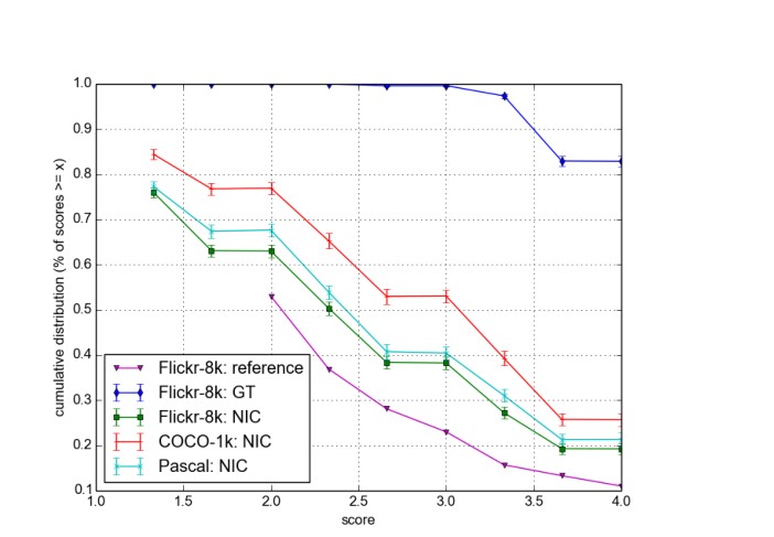
Figure 4. Flickr-8k: NIC: predictions produced by NIC on the Flickr8k test set (average score: 2.37); Pascal: NIC: (average score: 2.45); COCO-1k: NIC: A subset of 1000 images from the MSCOCO test set with descriptions produced by NIC (average score: 2.72); Flickr-8k: ref: these are results from [11] on Flickr8k rated using the same protocol, as a baseline (average score: 2.08); Flickr-8k: GT: we rated the groundtruth labels from Flickr8k using the same protocol. This provides us with a “calibration” of the scores (average score: 3.89)

图 4. Flickr-8k: NIC：NIC 在 Flickr8k 测试集上给出的预测（平均分 2.37）；Pascal: NIC：（平均分 2.45）；COCO-1k: NIC：从 MSCOCO 测试集取出的 1000 张图像子集，描述由 NIC 生成（平均分 2.72）；Flickr-8k: ref：来自 [11] 在 Flickr8k 上、按同一协议评分的结果，作为基线（平均分 2.08）；Flickr-8k: GT：我们用同一协议给 Flickr8k 的真值标注打分。这为分数提供了一种「校准」（平均分 3.89）。

4.3.6 Human Evaluation

4.3.6 人工评价

Figure 4 shows the result of the human evaluations of the descriptions provided by NIC, as well as a reference system and groundtruth on various datasets. We can see that NIC is better than the reference system, but clearly worse than the groundtruth, as expected. This shows that BLEU is not a perfect metric, as it does not capture well the difference between NIC and human descriptions assessed by raters. Examples of rated images can be seen in Figure 5. It is interesting to see, for instance in the second image of the first column, how the model was able to notice the frisbee given its size.

图 4 给出了对 NIC 所给描述的人工评价，以及参考系统和真值在多套数据上的结果。可以看到 NIC 好于参考系统，但正如所料，明显不如真值。这说明 BLEU 并不是完美的指标，因为它没有很好地抓住评分人所看到的 NIC 与人工描述之间的差别。被评分的图像例子见图 5。有意思的是，例如第一列第二张图，模型在飞盘很小的情况下仍然注意到了它。

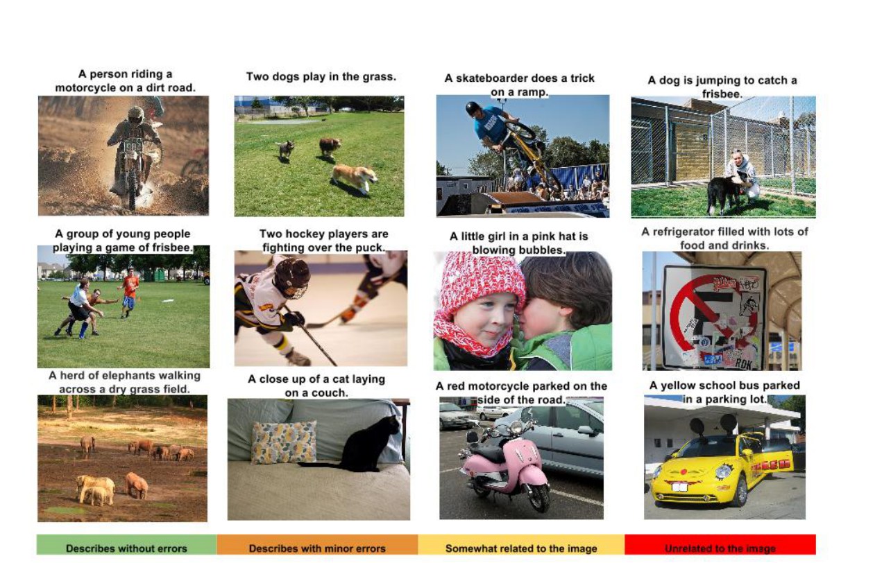
Figure 5. A selection of evaluation results, grouped by human rating.

图 5. 一组评价结果，按人工评分分组。

4.3.7 Analysis of Embeddings

4.3.7 对嵌入的分析

In order to represent the previous word S_{t−1} as input to the decoding LSTM producing S_t, we use word embedding vectors [22], which have the advantage of being independent of the size of the dictionary (contrary to a simpler one-hot-encoding approach). Furthermore, these word embeddings can be jointly trained with the rest of the model. It is remarkable to see how the learned representations have captured some semantic from the statistics of the language. Table 4.3.7 shows, for a few example words, the nearest other words found in the learned embedding space.

为了把前一个词 S_{t−1} 作为输入送给生成 S_t 的解码 LSTM，我们使用词嵌入向量 [22]，其好处是与词典大小无关（这与更简单的 one-hot 编码不同）。而且这些词嵌入可以和模型其余部分一起联合训练。值得注意的是，学到的表示已经从语言的统计里抓住了一些语义。表 4.3.7 给出若干例子词在学到的嵌入空间里最近的其他词。

Note how some of the relationships learned by the model will help the vision component. Indeed, having “horse”, “pony”, and “donkey” close to each other will encourage the CNN to extract features that are relevant to horse-looking animals. We hypothesize that, in the extreme case where we see very few examples of a class (e.g., “unicorn”), its proximity to other word embeddings (e.g., “horse”) should provide a lot more information that would be completely lost with more traditional bag-of-words based approaches.

可以看到，模型学到的某些关系会对视觉部分有帮助。的确，若 “horse”、“pony” 和 “donkey” 彼此靠近，就会促使 CNN 提取与像马的动物相关的特征。我们猜想，在某一类例子极少的极端情形下（例如 “unicorn”），它与其他词嵌入（例如 “horse”）的接近，应当能提供更多信息；而这些信息在更传统的词袋方法里会完全丢失。

Word	Neighbors
car	van, cab, suv, vehicule, jeep
boy	toddler, gentleman, daughter, son
street	road, streets, highway, freeway
horse	pony, donkey, pig, goat, mule
computer	computers, pc, crt, chip, compute

词	近邻
car	van, cab, suv, vehicule, jeep
boy	toddler, gentleman, daughter, son
street	road, streets, highway, freeway
horse	pony, donkey, pig, goat, mule
computer	computers, pc, crt, chip, compute

Table 6. Nearest neighbors of a few example words

表 6. 若干例子词的最近邻

5. Conclusion

5. 结论

We have presented NIC, an end-to-end neural network system that can automatically view an image and generate a reasonable description in plain English. NIC is based on a convolution neural network that encodes an image into a compact representation, followed by a recurrent neural network that generates a corresponding sentence. The model is trained to maximize the likelihood of the sentence given the image. Experiments on several datasets show the robustness of NIC in terms of qualitative results (the generated sentences are very reasonable) and quantitative evaluations, using either ranking metrics or BLEU, a metric used in machine translation to evaluate the quality of generated sentences. It is clear from these experiments that, as the size of the available datasets for image description increases, so will the performance of approaches like NIC. Furthermore, it will be interesting to see how one can use unsupervised data, both from images alone and text alone, to improve image description approaches.

我们介绍了 NIC：一个端到端的神经网络系统，能够自动查看一张图像，并生成一句还算合理的英文描述。NIC 的基础是一个把图像编成紧凑表示的卷积神经网络，后面再接一个生成对应句子的循环神经网络。模型的训练目标是最大化句子在给定图像时的似然。在多套数据上的实验表明，NIC 在定性结果（生成的句子相当合理）和定量评价上都比较稳健，定量指标既可以是排序指标，也可以是机器翻译里用来评价生成句质量的 BLEU。这些实验清楚表明：随着可用于图像描述的数据规模增大，像 NIC 这样的方法，表现也会随之提高。此外，如何同时利用仅有图像和仅有文本的无监督数据来改进图像描述方法，也将是一件有意思的事。

References

参考文献

[1] A. Aker and R. Gaizauskas. Generating image descriptions using dependency relational patterns. In ACL, 2010. 2

[2] D. Bahdanau, K. Cho, and Y. Bengio. Neural machine translation by jointly learning to align and translate. arXiv:1409.0473, 2014. 1, 2

[3] K. Cho, B. van Merrienboer, C. Gulcehre, F. Bougares, H. Schwenk, and Y. Bengio. Learning phrase representations using RNN encoder-decoder for statistical machine translation. In EMNLP, 2014. 1, 2, 3

[4] J. Donahue, Y. Jia, O. Vinyals, J. Hoffman, N. Zhang, E. Tzeng, and T. Darrell. Decaf: A deep convolutional activation feature for generic visual recognition. In ICML, 2014. 3

[5] D. Elliott and F. Keller. Image description using visual dependency representations. In EMNLP, 2013. 2

[6] A. Farhadi, M. Hejrati, M. A. Sadeghi, P. Young, C. Rashtchian, J. Hockenmaier, and D. Forsyth. Every picture tells a story: Generating sentences from images. In ECCV, 2010. 1, 2, 5

[7] R. Gerber and H.-H. Nagel. Knowledge representation for the generation of quantified natural language descriptions of vehicle traffic in image sequences. In ICIP. IEEE, 1996. 2

[8] Y. Gong, L. Wang, M. Hodosh, J. Hockenmaier, and S. Lazebnik. Improving image-sentence embeddings using large weakly annotated photo collections. In ECCV, 2014. 2, 5

[9] A. Graves. Generating sequences with recurrent neural networks. arXiv:1308.0850, 2013. 3

[10] S. Hochreiter and J. Schmidhuber. Long short-term memory. Neural Computation, 9(8), 1997. 2, 3

[11] M. Hodosh, P. Young, and J. Hockenmaier. Framing image description as a ranking task: Data, models and evaluation metrics. JAIR, 47, 2013. 2, 4, 6, 7

[12] S. Ioffe and C. Szegedy. Batch normalization: Accelerating deep network training by reducing internal covariate shift. In arXiv:1502.03167, 2015. 2, 3, 4

[13] A. Karpathy, A. Joulin, and L. Fei-Fei. Deep fragment embeddings for bidirectional image sentence mapping. NIPS, 2014. 2, 7

[14] R. Kiros, R. Salakhutdinov, and R. S. Zemel. Unifying visual-semantic embeddings with multimodal neural language models. In arXiv:1411.2539, 2014. 2, 5, 6, 7

[15] R. Kiros and R. Z. R. Salakhutdinov. Multimodal neural language models. In NIPS Deep Learning Workshop, 2013. 2

[16] G. Kulkarni, V. Premraj, S. Dhar, S. Li, Y. Choi, A. C. Berg, and T. L. Berg. Baby talk: Understanding and generating simple image descriptions. In CVPR, 2011. 1, 2, 6

[17] P. Kuznetsova, V. Ordonez, A. C. Berg, T. L. Berg, and Y. Choi. Collective generation of natural image descriptions. In ACL, 2012. 2

[18] P. Kuznetsova, V. Ordonez, T. Berg, and Y. Choi. Treetalk: Composition and compression of trees for image descriptions. ACL, 2(10), 2014. 2, 5, 6

[19] S. Li, G. Kulkarni, T. L. Berg, A. C. Berg, and Y. Choi. Composing simple image descriptions using web-scale n-grams. In Conference on Computational Natural Language Learning, 2011. 2

[20] T.-Y. Lin, M. Maire, S. Belongie, J. Hays, P. Perona, D. Ramanan, P. Dollár, and C. L. Zitnick. Microsoft coco: Common objects in context. arXiv:1405.0312, 2014. 5

[21] J. Mao, W. Xu, Y. Yang, J. Wang, and A. Yuille. Explain images with multimodal recurrent neural networks. In arXiv:1410.1090, 2014. 2, 6, 7

[22] T. Mikolov, K. Chen, G. Corrado, and J. Dean. Efficient estimation of word representations in vector space. In ICLR, 2013. 6, 8

[23] M. Mitchell, X. Han, J. Dodge, A. Mensch, A. Goyal, A. C. Berg, K. Yamaguchi, T. L. Berg, K. Stratos, and H. D. III. Midge: Generating image descriptions from computer vision detections. In EACL, 2012. 2

[24] V. Ordonez, G. Kulkarni, and T. L. Berg. Im2text: Describing images using 1 million captioned photographs. In NIPS, 2011. 2, 5, 6

[25] K. Papineni, S. Roukos, T. Ward, and W. J. Zhu. BLEU: A method for automatic evaluation of machine translation. In ACL, 2002. 4

[26] C. Rashtchian, P. Young, M. Hodosh, and J. Hockenmaier. Collecting image annotations using amazon’s mechanical turk. In NAACL HLT Workshop on Creating Speech and Language Data with Amazon’s Mechanical Turk, pages 139–147, 2010. 5

[27] O. Russakovsky, J. Deng, H. Su, J. Krause, S. Satheesh, S. Ma, Z. Huang, A. Karpathy, A. Khosla, M. Bernstein, A. C. Berg, and L. Fei-Fei. ImageNet Large Scale Visual Recognition Challenge, 2014. 1

[28] P. Sermanet, D. Eigen, X. Zhang, M. Mathieu, R. Fergus, and Y. LeCun. Overfeat: Integrated recognition, localization and detection using convolutional networks. arXiv preprint arXiv:1312.6229, 2013. 2

[29] R. Socher, A. Karpathy, Q. V. Le, C. Manning, and A. Y. Ng. Grounded compositional semantics for finding and describing images with sentences. In ACL, 2014. 2

[30] I. Sutskever, O. Vinyals, and Q. V. Le. Sequence to sequence learning with neural networks. In NIPS, 2014. 1, 2, 3

[31] R. Vedantam, C. L. Zitnick, and D. Parikh. CIDEr: Consensus-based image description evaluation. In arXiv:1411.5726, 2015. 5, 6

[32] B. Z. Yao, X. Yang, L. Lin, M. W. Lee, and S.-C. Zhu. I2t: Image parsing to text description. Proceedings of the IEEE, 98(8), 2010. 2

[33] P. Young, A. Lai, M. Hodosh, and J. Hockenmaier. From image descriptions to visual denotations: New similarity metrics for semantic inference over event descriptions. In ACL, 2014. 5

[34] W. Zaremba, I. Sutskever, and O. Vinyals. Recurrent neural network regularization. In arXiv:1409.2329, 2014. 6