A Unified Approach to Interpreting Model Predictions

一种统一的模型预测解释方法

Scott M. Lundberg
Paul G. Allen School of Computer Science
University of Washington
Seattle, WA 98105
slund1@cs.washington.edu

Su-In Lee
Paul G. Allen School of Computer Science
Department of Genome Sciences
University of Washington
Seattle, WA 98105
suinlee@cs.washington.edu

Abstract

摘要

Understanding why a model makes a certain prediction can be as crucial as the prediction’s accuracy in many applications. However, the highest accuracy for large modern datasets is often achieved by complex models that even experts struggle to interpret, such as ensemble or deep learning models, creating a tension between accuracy and interpretability. In response, various methods have recently been proposed to help users interpret the predictions of complex models, but it is often unclear how these methods are related and when one method is preferable over another. To address this problem, we present a unified framework for interpreting predictions, SHAP (SHapley Additive exPlanations). SHAP assigns each feature an importance value for a particular prediction. Its novel components include: (1) the identification of a new class of additive feature importance measures, and (2) theoretical results showing there is a unique solution in this class with a set of desirable properties. The new class unifies six existing methods, notable because several recent methods in the class lack the proposed desirable properties. Based on insights from this unification, we present new methods that show improved computational performance and/or better consistency with human intuition than previous approaches.

在许多应用里，弄清模型为什么给出某次预测，其重要性并不亚于预测本身准不准。可是，在当今大规模数据上往往最准的是集成模型或深度学习这类复杂模型，连专家也很难解释，于是精度和可解释性之间出现了张力。作为回应，近来已经有多种方法帮助使用者解释复杂模型的预测，但这些方法彼此如何关联、何时一种方法更合适，常常并不清楚。为解决这个问题，我们提出一套统一的预测解释框架 SHAP（SHapley Additive exPlanations）。SHAP 为某一次预测中的每个特征赋一个重要性值。其新意主要包括：（1）识别出一类新的可加特征重要性度量；（2）从理论上证明，在这类度量中，满足一组理想性质的解是唯一的。这个新类把已有的六种方法统一到一起，这一点值得注意，因为其中若干近期方法并不具备文中提出的那些理想性质。基于这一统一带来的认识，我们提出新的方法，它们在计算效率上优于已有做法，并且／或者与人类直觉更一致。

1 Introduction

1 引言

The ability to correctly interpret a prediction model’s output is extremely important. It engenders appropriate user trust, provides insight into how a model may be improved, and supports understanding of the process being modeled. In some applications, simple models (e.g., linear models) are often preferred for their ease of interpretation, even if they may be less accurate than complex ones. However, the growing availability of big data has increased the benefits of using complex models, so bringing to the forefront the trade-off between accuracy and interpretability of a model’s output. A wide variety of different methods have been recently proposed to address this issue [5, 8, 9, 3, 4, 1]. But an understanding of how these methods relate and when one method is preferable to another is still lacking.

正确解释预测模型的输出极为重要。它能带来恰当的使用者信任，提供如何改进模型的线索，也有助于理解被建模的过程。在一些应用中，人们常常更愿意用简单模型（例如线性模型），因为它们容易解释，即便精度可能不如复杂模型。然而，随着大数据越来越容易获得，使用复杂模型的好处也在增加，模型输出的精度与可解释性之间的权衡因此被推到台前。近来已有多种不同方法试图应对这一问题 [5, 8, 9, 3, 4, 1]。但这些方法如何相互关联，以及何时一种方法优于另一种，人们仍然缺少清楚的认识。

Here, we present a novel unified approach to interpreting model predictions.[^1] Our approach leads to three potentially surprising results that bring clarity to the growing space of methods:

在此，我们提出一种新的、统一的模型预测解释方法。[^1] 这一方法带来三个可能出人意料的结果，为日益增多的方法澄清了关系：

1. We introduce the perspective of viewing any explanation of a model’s prediction as a model itself, which we term the explanation model. This lets us define the class of additive feature attribution methods (Section 2), which unifies six current methods.

1. 我们引入这样一种视角：把对模型某次预测的任何解释本身也看成一个模型，并称之为解释模型（explanation model）。由此可以定义可加特征归因方法（additive feature attribution methods）这一类（第 2 节），并把当前的六种方法统一进来。

2. We then show that game theory results guaranteeing a unique solution apply to the entire class of additive feature attribution methods (Section 3) and propose SHAP values as a unified measure of feature importance that various methods approximate (Section 4).

2. 接着我们证明，保证唯一解的博弈论结果适用于整个可加特征归因方法类（第 3 节），并提出 SHAP 值，作为各种方法都在逼近的统一特征重要性度量（第 4 节）。

3. We propose new SHAP value estimation methods and demonstrate that they are better aligned with human intuition as measured by user studies and more effectually discriminate among model output classes than several existing methods (Section 5).

3. 我们提出新的 SHAP 值估计方法，并表明它们在用户研究中与人类直觉更一致，也比若干已有方法更能有效地区分模型的输出类别（第 5 节）。

2 Additive Feature Attribution Methods

2 可加特征归因方法

The best explanation of a simple model is the model itself; it perfectly represents itself and is easy to understand. For complex models, such as ensemble methods or deep networks, we cannot use the original model as its own best explanation because it is not easy to understand. Instead, we must use a simpler explanation model, which we define as any interpretable approximation of the original model. We show below that six current explanation methods from the literature all use the same explanation model. This previously unappreciated unity has interesting implications, which we describe in later sections.

对简单模型最好的解释就是模型自己：它完美地表示自身，也容易理解。对集成方法或深度网络这类复杂模型，我们不能把原模型当作它自己最好的解释，因为它不容易懂。于是必须使用更简单的解释模型，我们把它定义为对原模型的任何可解释近似。下面将表明，文献中现有的六种解释方法都使用同一种解释模型。这一此前未被重视的统一有一些有趣的含义，我们将在后面几节讨论。

Let $f$ be the original prediction model to be explained and $g$ the explanation model. Here, we focus on local methods designed to explain a prediction $f(x)$ based on a single input $x$, as proposed in LIME [5]. Explanation models often use simplified inputs $x^{\prime}$ that map to the original inputs through a mapping function $x=h_{x}(x^{\prime})$. Local methods try to ensure $g(z^{\prime})\approx f(h_{x}(z^{\prime}))$ whenever $z^{\prime}\approx x^{\prime}$. (Note that $h_{x}(x^{\prime})=x$ even though $x^{\prime}$ may contain less information than $x$ because $h_{x}$ is specific to the current input $x$.)

设 $f$ 是有待解释的原预测模型，$g$ 是解释模型。这里我们关注用于解释单个输入 $x$ 上的预测 $f(x)$ 的局部方法，正如 LIME [5] 所提出的。解释模型常常使用简化输入 $x'$，再通过映射函数 $x=h_x(x')$ 映回原始输入。局部方法试图保证：只要 $z'\approx x'$，就有 $g(z')\approx f(h_x(z'))$。（注意，即便 $x'$ 所含信息可能少于 $x$，仍有 $h_x(x')=x$，因为 $h_x$ 是针对当前输入 $x$ 的。）

Definition 1

Additive feature attribution methodshave an explanation model that is a linear function of binary variables:

定义 1

$$g(z^{\prime})=\phi_{0}+\sum_{i=1}^{M}\phi_{i}z_{i}^{\prime}, \tag{1}$$

where $z^{\prime}\in\{0,1\}^{M}$, $M$ is the number of simplified input features, and $\phi_{i}\in\mathbb{R}$.

其中 $z'\in\{0,1\}^{M}$，$M$ 是简化输入特征的个数，$\phi_i\in\mathbb{R}$。

Methods with explanation models matching Definition 1 attribute an effect $\phi_{i}$ to each feature, and summing the effects of all feature attributions approximates the output $f(x)$ of the original model. Many current methods match Definition 1, several of which are discussed below.

符合定义 1 的方法把效应 $\phi_i$ 归于每个特征，所有特征效应之和逼近原模型在 $f(x)$ 上的输出。把 $z_i'=1$ 解释为该特征被观察到，$z_i'=0$ 解释为未知，是常见但并非必须的约定。

2.1 LIME

The LIME method interprets individual model predictions based on locally approximating the model around a given prediction [5]. The local linear explanation model that LIME uses adheres to Equation 1 exactly and is thus an additive feature attribution method. LIME refers to simplified inputs $x^{\prime}$ as “interpretable inputs,” and the mapping $x=h_{x}(x^{\prime})$ converts a binary vector of interpretable inputs into the original input space. Different types of $h_{x}$ mappings are used for different input spaces. For bag of words text features, $h_{x}$ converts a vector of $1$’s or $0$’s (present or not) into the original word count if the simplified input is one, or zero if the simplified input is zero. For images, $h_{x}$ treats the image as a set of super pixels; it then maps $1$ to leaving the super pixel as its original value and $0$ to replacing the super pixel with an average of neighboring pixels (this is meant to represent being missing).

LIME 方法基于对原模型的局部近似来解释单次模型预测。文中作者提议用各种解释模型 $g$ 做这种近似，并用多种损失函数 $L$ 和正则化项度量这种近似。这里我们关注使用作者所谓稀疏线性解释模型的 LIME，也是他们唯一用于展示和对比的解释模型。这一种 LIME 使用可加特征归因方法的解释模型（定义 1），其中 $x'$ 将原始输入映射到 $\{0,1\}^M$，而 $h_x$ 把 $1$ 映回原始输入中对应的值，把 $0$ 映回另一基值，例如均值。

To find $\phi$, LIME minimizes the following objective function:

为了求出 $\phi$，LIME 最小化下面的目标函数：

$$\xi=\mathop{{\arg\min}\vphantom{\sim}}\limits_{{}_{g\in\mathcal{G}}}~L(f,g,\pi_{x^{\prime}})+\Omega(g). \tag{2}$$

$$\xi=\mathop{{\arg\min}\vphantom{\sim}}\limits_{{}_{g\in\mathcal{G}}}~L(f,g,\pi_{x'})+\Omega(g) \tag{2}$$

Faithfulness of the explanation model $g(z^{\prime})$ to the original model $f(h_{x}(z^{\prime}))$ is enforced through the loss $L$ over a set of samples in the simplified input space weighted by the local kernel $\pi_{x^{\prime}}$. $\Omega$ penalizes the complexity of $g$. Since in LIME $g$ follows Equation 1 and $L$ is a squared loss, Equation 2 can be solved using penalized linear regression.

解释模型 $g(z')$ 对原模型 $f(h_x(z'))$ 的忠实程度，由损失函数 $L$ 在由局部核 $\pi_{x'}$ 加权的样本上施加。由于在 LIME 中 $\Omega$、$\pi$ 和 $L$ 的选择都带有启发性，即便是为了改进公平性而做的调整，也并不总是能恢复到与人类直觉一致的解，第 5 节会给出例子。

2.2 DeepLIFT

DeepLIFT was recently proposed as a recursive prediction explanation method for deep learning [8, 7]. It attributes to each input $x_{i}$ a value $C_{\Delta x_{i}\Delta y}$ that represents the effect of that input being set to a reference value as opposed to its original value. This means that for DeepLIFT, the mapping $x=h_{x}(x^{\prime})$ converts binary values into the original inputs, where $1$ indicates that an input takes its original value, and $0$ indicates that it takes the reference value. The reference value, though chosen by the user, represents a typical uninformative background value for the feature.

DeepLIFT 最近被提出，作为一种面向深度网络的递归预测解释方法 [8]。它把差值归因于所有输入特征的相对变化，而这个差值是相对于某个参考值而言的。DeepLIFT 也属于可加特征归因方法，其简化输入 $x'$ 表示输入中的二值指示：某个输入要么取原始值，要么取参考值（方程 1）。DeepLIFT 用线性组合规则把模型中每个非线性单元上的差值近似分配下去。各分量的效应 $\phi_i$ 对应于每个输入的归因量 $C_{\Delta x_i \Delta o}$。

DeepLIFT uses a "summation-to-delta" property that states:

DeepLIFT 使用一条“对差值求和”性质，其表述为：

$$\sum_{i=1}^{n}C_{\Delta x_{i}\Delta o}=\Delta o, \tag{3}$$

where $o=f(x)$ is the model output, $\Delta o=f(x)-f(r)$, $\Delta x_{i}=x_{i}-r_{i}$, and $r$ is the reference input. If we let $\phi_{i}=C_{\Delta x_{i}\Delta o}$ and $\phi_{0}=f(r)$, then DeepLIFT’s explanation model matches Equation 1 and is thus another additive feature attribution method.

其中 $o=f(x)$ 是模型输出，$\Delta o=f(x)-f(r)$，$\Delta x_i=x_i-r_i$，$r$ 是参考输入。可以把方程 3 改写成定义 1 的形式：令 $\phi_i=C_{\Delta x_i\Delta o}$，$\phi_0=f(r)$，就与方程 3 以及 $z_i'=1_{x_i\neq r_i}$ 相一致。

2.3 Layer-Wise Relevance Propagation

2.3 逐层相关性传播

The layer-wise relevance propagation method interprets the predictions of deep networks [1]. As noted by [8], this menthod is equivalent to DeepLIFT with the reference activations of all neurons fixed to zero. Thus, $x=h_{x}(x^{\prime})$ converts binary values into the original input space, where $1$ means that an input takes its original value, and $0$ means an input takes the $0$ value. Layer-wise relevance propagation’s explanation model, like DeepLIFT’s, matches Equation 1.

逐层相关性传播（layer-wise relevance propagation）方法解释深度网络的预测 [1]。该技术沿着网络反向操作，把每次预测的解释重新分配到每一个输入。其简化输入表示一个输入是否取了参考值，而该参考值被设为 $0$。于是，相关性传播的递推规则给出的值 $R_i$ 可以视为满足定义 1 的值 $\phi_i$，其中 $z_i'=1_{x_i\neq 0}$。

2.4 Classic Shapley Value Estimation

2.4 经典 Shapley 值估计

Three previous methods use classic equations from cooperative game theory to compute explanations of model predictions: Shapley regression values [4], Shapley sampling values [9], and Quantitative Input Influence [3].

先前已有三种方法用合作博弈论中的经典方程来计算 $g$ 的解，而不是像前面的方法那样设法用启发式规则来避免它。

Shapley regression values are feature importances for linear models in the presence of multicollinearity. This method requires retraining the model on all feature subsets $S\subseteq F$, where $F$ is the set of all features. It assigns an importance value to each feature that represents the effect on the model prediction of including that feature. To compute this effect, a model $f_{S\cup\{i\}}$ is trained with that feature present, and another model $f_{S}$ is trained with the feature withheld. Then, predictions from the two models are compared on the current input $f_{S\cup\{i\}}(x_{S\cup\{i\}})-f_{S}(x_{S})$, where $x_{S}$ represents the values of the input features in the set $S$. Since the effect of withholding a feature depends on other features in the model, the preceding differences are computed for all possible subsets $S\subseteq F\setminus\{i\}$. The Shapley values are then computed and used as feature attributions. They are a weighted average of all possible differences:

Shapley 回归值是存在特征多重共线性时线性模型的特征重要性，其计算来自每个特征在所有可能特征子集上的边际贡献的加权平均 [4]。Shapley 回归值对应于定义 1 中的特征归因，而其中的 $h_x$ 把 $1$ 或 $0$ 映回原始输入或某个基值。

$$\phi_{i}=\sum_{S\subseteq F\setminus\{i\}}\frac{|S|!(|F|-|S|-1)!}{|F|!}\left[f_{S\cup\{i\}}(x_{S\cup\{i\}})-f_{S}(x_{S})\right]. \tag{4}$$

$$\phi_{i}=\sum_{S\subseteq F\setminus\{i\}}\frac{|S|!(|F|-|S|-1)!}{|F|!}\left[f_{S\cup\{i\}}(x_{S\cup\{i\}})-f_{S}(x_{S})\right] \tag{4}$$

For Shapley regression values, $h_{x}$ maps $1$ or $0$ to the original input space, where $1$ indicates the input is included in the model, and $0$ indicates exclusion from the model. If we let $\phi_{0}=f_{\varnothing}(\varnothing)$, then the Shapley regression values match Equation 1 and are hence an additive feature attribution method.

对 Shapley 回归值而言，$h_x$ 把 $1$ 或 $0$ 映回原始输入空间，缺失特征用对可能取值的积分来表示。$F$ 是所有特征的集合，$S$ 是 $F$ 中不含特征 $i$ 的子集，$f_{S}$ 是只在 $S$ 中特征上训练的模型。

Shapley sampling values are meant to explain any model by: (1) applying sampling approximations to Equation 4, and (2) approximating the effect of removing a variable from the model by integrating over samples from the training dataset. This eliminates the need to retrain the model and allows fewer than $2^{|F|}$ differences to be computed. Since the explanation model form of Shapley sampling values is the same as that for Shapley regression values, it is also an additive feature attribution method.

Shapley 采样值旨在解释任意模型，做法是：（1）把经典 Shapley 方程（方程 4）中的 $f_{S\cup\{i\}}(x_{S\cup\{i\}})-f_S(x_S)$ 项换成对随机实例中缺失特征做抽样后的差值；（2）对求和做近似，只使用特征排列的一个子集 [9]。这同样属于可加特征归因方法，其简化输入表示一个输入是否被纳入抽样的近似。

Quantitative input influence is a broader framework that addresses more than feature attributions. However, as part of its method it independently proposes a sampling approximation to Shapley values that is nearly identical to Shapley sampling values. It is thus another additive feature attribution method.

定量输入影响（quantitative input influence）是一个更宽的框架，讨论的不止是特征归因，其中一个选项就是用抽样来近似 Shapley 值，这和 Shapley 采样值非常接近 [3]。

3 Simple Properties Uniquely Determine Additive Feature Attributions

3 若干简单性质唯一确定可加特征归因

A surprising attribute of the class of additive feature attribution methods is the presence of a single unique solution in this class with three desirable properties (described below). While these properties are familiar to the classical Shapley value estimation methods, they were previously unknown for other additive feature attribution methods.

可加特征归因方法这一类有一个出人意料的属性：只有一个解满足三个我们看来很自然的性质。这一节把这些性质和对应的唯一解形式化。

The first desirable property is local accuracy. When approximating the original model $f$ for a specific input $x$, local accuracy requires the explanation model to at least match the output of $f$ for the simplified input $x^{\prime}$ (which corresponds to the original input $x$).

第一条理想性质是局部准确（local accuracy）。在用解释模型逼近原模型时，我们希望至少在被解释的那一点上与原模型完全吻合。

Property 1(Local accuracy)

$$f(x)=g(x^{\prime})=\phi_{0}+\sum_{i=1}^{M}\phi_{i}x_{i}^{\prime} \tag{5}$$

性质 1（局部准确）

$$f(x)=g(x^{\prime})=\phi_{0}+\sum_{i=1}^{M}\phi_{i}x_{i}^{\prime} \tag{5}$$

The explanation model $g(x')$ matches the original model $f(x)$ when $x=h_x(x')$, where $\phi_0=f(h_x(0))$ represents the model output with all simplified inputs toggled off (i.e. missing).

当 $x=h_x(x')$ 时，解释模型 $g(x')$ 与原模型 $f(x)$ 相一致，其中 $\phi_0=f(h_x(0))$ 表示所有简化输入都被关掉（也即缺失）时的模型输出。

The second property is missingness. If the simplified inputs represent feature presence, then missingness requires features missing in the original input to have no impact. All of the methods described in Section 2 obey the missingness property.

第二条性质是缺失（missingness）。如果简化输入表示的是特征是否出现，那么缺失性要求：在原始输入中已经缺失的特征不应产生影响。第 2 节描述的方法都允许缺失性。

Property 2(Missingness)

$$x^{\prime}_{i}=0\implies\phi_{i}=0 \tag{6}$$

性质 2（缺失）

$$x^{\prime}_{i}=0\implies\phi_{i}=0 \tag{6}$$

Missingness constrains features where $x^{\prime}_{i}=0$ to have no attributed impact.

缺失性约束了 $x'_i=0$ 的特征，使其没有被归因的影响。

The third property is consistency. Consistency states that if a model changes so that some simplified input’s contribution increases or stays the same regardless of the other inputs, that input’s attribution should not decrease.

第三条性质是一致性（consistency）。一致性说的是：如果一个模型发生改变，使某个简化输入的贡献增大或保持不变（不论其他输入如何），则该输入的归因不应下降。

Property 3(Consistency)

Let $f_{x}(z^{\prime})=f(h_{x}(z^{\prime}))$ and $z^{\prime}\setminus i$ denote setting $z^{\prime}_{i}=0$. For any two models $f$ and $f^{\prime}$, if

性质 3（一致性）

设 $f_x(z')=f(h_x(z'))$，并用 $z'\setminus i$ 表示令 $z'_i=0$。对任意两个模型 $f$ 和 $f'$，若

$$f^{\prime}_{x}(z^{\prime})-f^{\prime}_{x}(z^{\prime}\setminus i)\geq f_{x}(z^{\prime})-f_{x}(z^{\prime}\setminus i) \tag{7}$$

for all inputs $z^{\prime}\in\{0,1\}^{M}$, then $\phi_{i}(f^{\prime},x)\geq\phi_{i}(f,x)$.

对所有输入 $z'\in\{0,1\}^{M}$ 都成立，则 $\phi_i(f',x)\geq\phi_i(f,x)$。

Theorem 1

Only one possible explanation model $g$ follows Definition 1 and satisfies Properties 1, 2, and 3:

定理 1

只有一种可能的解释模型 $g$ 既符合定义 1，又满足性质 1、2 和 3：

$$\phi_{i}(f,x)=\sum_{z^{\prime}\subseteq x^{\prime}}\frac{|z^{\prime}|!(M-|z^{\prime}|-1)!}{M!}\left[f_{x}(z^{\prime})-f_{x}(z^{\prime}\setminus i)\right] \tag{8}$$

where $|z^{\prime}|$ is the number of non-zero entries in $z^{\prime}$, and $z^{\prime}\subseteq x^{\prime}$ represents all $z^{\prime}$ vectors where the non-zero entries are a subset of the non-zero entries in $x^{\prime}$.

其中 $|z'|$ 是 $z'$ 中非零项的个数，$z'\subseteq x'$ 表示 $z'$ 的非零项是 $x'$ 非零项的子集。

Theorem 1 follows from combined cooperative game theory results, where the values $\phi_{i}$ are known as Shapley values [6]. [10] (1985) demonstrated that Shapley values are the only set of values that satisfy three axioms similar to Property 1, Property 3, and a final property that we show to be redundant in this setting (see Supplementary Material). Property 2 is required to adapt the Shapley proofs to the class of additive feature attribution methods.

定理 1 来自合作博弈论结果的结合，其中 $\phi_i$ 被称为 Shapley 值。Young [10] 给出的结果证明了 Shapley 值是唯一满足与性质 1、性质 3 以及另一条性质相似的三条公理的归因，而那条额外性质在本文设定下是冗余的（见补充材料）。性质 2 则是为了把 Shapley 值适配到定义 1 所需要的，在博弈论文献中通常是隐含的。

Under Properties 1-3, for a given simplified input mapping $h_{x}$, Theorem 1 shows that there is only one possible additive feature attribution method. This result implies that methods not based on Shapley values violate local accuracy and/or consistency (methods in Section 2 already respect missingness). The following section proposes a unified approach that improves previous methods, preventing them from unintentionally violating Properties 1 and 3.

在性质 1–3 之下，对给定的简化输入映射 $h_x$，定理 1 表明只有一种可能的可加特征归因方法。这个方法就是第 2 节描述的 Shapley 回归、Shapley 采样和定量输入影响方法所追求的（当 $h_x$ 把 $x'$ 映回原始输入空间时）。

4 SHAP (SHapley Additive exPlanation) Values

4 SHAP（SHapley Additive exPlanation）值

We propose SHAP values as a unified measure of feature importance. These are the Shapley values of a conditional expectation function of the original model; thus, they are the solution to Equation 8, where $f_{x}(z^{\prime})=f(h_{x}(z^{\prime}))=E[f(z)\mid z_{S}]$, and $S$ is the set of non-zero indexes in $z^{\prime}$ (Figure 1). Based on Sections 2 and 3, SHAP values provide the unique additive feature importance measure that adheres to Properties 1-3 and uses conditional expectations to define simplified inputs. Implicit in this definition of SHAP values is a simplified input mapping, $h_{x}(z^{\prime})=z_{S}$, where $z_{S}$ has missing values for features not in the set $S$. Since most models cannot handle arbitrary patterns of missing input values, we approximate $f(z_{S})$ with $E[f(z)\mid z_{S}]$. This definition of SHAP values is designed to closely align with the Shapley regression, Shapley sampling, and quantitative input influence feature attributions, while also allowing for connections with LIME, DeepLIFT, and layer-wise relevance propagation.

我们提出用 SHAP 值作为统一的特征重要性度量。它们是原模型条件期望函数的 Shapley 值；因此，它们是方程 8 的解，其中 $f_x(z')=f(h_x(z'))=E[f(z)\mid z_S]$，$S$ 是 $z'$ 中非零下标的集合（图 1）。根据第 2、3 节，SHAP 值提供了唯一满足性质 1–3、并用条件期望来定义简化输入的可加特征重要性度量。这一定义里隐含了一个简化输入映射 $h_x(z')=z_S$，其中 $z_S$ 对不在集合 $S$ 中的特征取缺失值。由于多数模型无法处理任意缺失输入模式，我们用 $E[f(z)\mid z_S]$ 来近似 $f(z_S)$。SHAP 值的这一定义旨在与 Shapley 回归、Shapley 采样和定量输入影响的特征归因密切对齐，同时又允许与 LIME、DeepLIFT 以及逐层相关性传播建立联系。

The exact computation of SHAP values is challenging. However, by combining insights from current additive feature attribution methods, we can approximate them. We describe two model-agnostic approximation methods, one that is already known (Shapley sampling values) and another that is novel (Kernel SHAP). We also describe four model-type-specific approximation methods, two of which are novel (Max SHAP, Deep SHAP). When using these methods, feature independence and model linearity are two optional assumptions simplifying the computation of the expected values (note that $\bar{S}$ is the set of features not in $S$):

精确计算 SHAP 值很困难。不过，把现有可加特征归因方法中的认识结合起来，我们可以做近似。我们描述两种不依赖模型结构的近似方法，一种已为人所知（Shapley 采样值），另一种是新的（Kernel SHAP）。我们还描述四种面向特定模型类型的近似方法，其中两种是新的（Max SHAP、Deep SHAP）。使用这些方法时，特征独立和模型线性是两个可选假定，用来简化期望值的计算（注意 $\bar{S}$ 是不在 $S$ 中的特征集合）：

$$\begin{aligned}
f(h_x(z')) &= E[f(z)\mid z_S] && \text{SHAP explanation model simplified input mapping} \tag{9}\
&= E_{z_{\bar{S}}\mid z_S}[f(z)] && \text{expectation over } z_{\bar{S}}\mid z_S \tag{10}\
&\approx E_{z_{\bar{S}}}[f(z)] && \text{assume feature independence (as in [9, 5, 7, 3])} \tag{11}\
&\approx f([z_S, E[z_{\bar{S}}]]). && \text{assume model linearity} \tag{12}
\end{aligned}$$

$$\begin{aligned}
f(h_x(z')) &= E[f(z)\mid z_S] && \text{SHAP 解释模型的简化输入映射} \tag{9}\
&= E_{z_{\bar{S}}\mid z_S}[f(z)] && \text{对 } z_{\bar{S}}\mid z_S \text{ 取期望} \tag{10}\
&\approx E_{z_{\bar{S}}}[f(z)] && \text{假定特征独立（如 [9, 5, 7, 3]）} \tag{11}\
&\approx f([z_S, E[z_{\bar{S}}]]). && \text{假定模型线性} \tag{12}
\end{aligned}$$

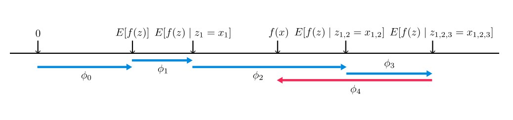
Figure 1: SHAP (SHapley Additive exPlanation) values attribute to each feature the change in the expected model prediction when conditioning on that feature. They explain how to get from the base value $E[f(z)]$ that would be predicted if we did not know any features to the current output $f(x)$. This diagram shows a single ordering. When the model is non-linear or the input features are not independent, however, the order in which features are added to the expectation matters, and the SHAP values arise from averaging the $\phi_i$ values across all possible orderings.

图 1：SHAP（SHapley Additive exPlanation）值把条件于该特征时模型期望预测的变化归因到每一个特征。它们解释的是：如何从假如我们一无所知时会预测的基准值 $E[f(z)]$，走到当前输出 $f(x)$。本图只画了一种排序。然而，当模型非线性或输入特征不独立时，特征被加入期望的顺序会影响结果，SHAP 值则来自对所有可能排序上 $\phi_i$ 的平均。

4.1 Model-Agnostic Approximations

4.1 不依赖模型结构的近似

If we assume feature independence when approximating conditional expectations (Equation 11), as in [9, 5, 7, 3], then SHAP values can be estimated directly using the Shapley sampling values method [9] or equivalently the Quantitative Input Influence method [3]. These methods use a sampling approximation of a permutation version of the classic Shapley value equations (Equation 8). Separate sampling estimates are performed for each feature attribution. While reasonable to compute for a small number of inputs, the Kernel SHAP method described next requires fewer evaluations of the original model to obtain similar approximation accuracy (Section 5).

如果在近似条件期望时假定特征独立（方程 11），正如 [9, 5, 7, 3] 所做的，那么 SHAP 值可以直接用 Shapley 采样值方法 [9]，或等价地用定量输入影响方法 [3] 来估计。这些方法对经典 Shapley 值方程（方程 8）的一种排列形式做抽样近似。每个特征归因都单独做抽样估计。对输入个数较少时这样算是合理的，但下一小节的 Kernel SHAP 要用更少的原模型评估次数，才能达到相近的近似精度（第 5 节）。

Kernel SHAP (Linear LIME + Shapley values)

Linear LIME uses a linear explanation model to locally approximate $f$, where local is measured in the simplified binary input space. At first glance, the regression formulation of LIME in Equation 2 seems very different from the classical Shapley value formulation of Equation 8. However, since linear LIME is an additive feature attribution method, we know the Shapley values are the only possible solution to Equation 2 that satisfies Properties 1-3 – local accuracy, missingness and consistency. A natural question to pose is whether the solution to Equation 2 recovers these values. The answer depends on the choice of loss function $L$, weighting kernel $\pi_{x^{\prime}}$ and regularization term $\Omega$. The LIME choices for these parameters are made heuristically; using these choices, Equation 2 does not recover the Shapley values. One consequence is that local accuracy and/or consistency are violated, which in turn leads to unintuitive behavior in certain circumstances (see Section 5).

Kernel SHAP（线性 LIME + Shapley 值）

线性 LIME 用线性解释模型在局部逼近 $f$，这里的“局部”是在简化后的二值输入空间里度量的。乍一看，方程 2 中 LIME 的回归形式与方程 8 中经典 Shapley 值的形式很不一样。可是，既然线性 LIME 是可加特征归因方法，我们就知道满足性质 1–3——局部准确、缺失和一致性——的方程 2 的解，只可能是 Shapley 值。一个自然的问题是：方程 2 的解会不会恢复这些值？答案取决于损失函数 $L$、加权核 $\pi_{x'}$ 和正则项 $\Omega$ 的选择。LIME 对这些参数的选择是启发式的；按这些选择，方程 2 并不能恢复 Shapley 值。一个后果是局部准确和／或一致性会被破坏，从而在某些情形下出现有违直觉的行为（见第 5 节）。

Below we show how to avoid heuristically choosing the parameters in Equation 2 and how to find the loss function $L$, weighting kernel $\pi_{x^{\prime}}$, and regularization term $\Omega$ that recover the Shapley values.

下面我们说明如何避免启发式地选择方程 2 中的参数，以及如何找到能恢复 Shapley 值的损失函数 $L$、加权核 $\pi_{x'}$ 和正则项 $\Omega$。

Theorem 2(Shapley kernel)

Under Definition 1, the specific forms of $\pi_{x^{\prime}}$, $L$, and $\Omega$ that make solutions of Equation 2 consistent with Properties 1 through 3 are:

定理 2（Shapley 核）

在定义 1 之下，使方程 2 的解与性质 1 至 3 相一致的 $\pi_{x'}$、$L$ 和 $\Omega$ 的具体形式是：

$$\begin{split}\Omega(g)&=0,\
\pi_{x^{\prime}}(z^{\prime})&=\frac{(M-1)}{(Mchoose|z^{\prime}|)|z^{\prime}|(M-|z^{\prime}|)},\
L(f,g,\pi_{x^{\prime}})&=\sum_{z^{\prime}\in Z}\left[f(h_{x}^{-1}(z^{\prime}))-g(z^{\prime})\right]^{2}\pi_{x^{\prime}}(z^{\prime}),\
\end{split}$$

where $|z^{\prime}|$ is the number of non-zero elements in $z^{\prime}$.

其中 $|z'|$ 是 $z'$ 中非零元素的个数。

The proof of Theorem 2 is shown in the Supplementary Material.

定理 2 的证明见补充材料。

It is important to note that $\pi_{x^{\prime}}(z^{\prime})=\infty$ when $|z^{\prime}|\in\{0,M\}$, which enforces $\phi_{0}=f_{x}(\varnothing)$ and $f(x)=\sum_{i=0}^{M}\phi_{i}$. In practice, these infinite weights can be avoided during optimization by analytically eliminating two variables using these constraints.

需要注意的是，当 $|z'|\in\{0,M\}$ 时 $\pi_{x'}(z')=\infty$，这强制了 $\phi_0=f_x(\varnothing)$ 以及 $f(x)=\sum_{i=0}^{M}\phi_i$。在优化时，可以利用这些约束用解析方法消去两个变量，从而避开无穷权重。

Since $g(z^{\prime})$ in Theorem 2 is assumed to follow a linear form, and $L$ is a squared loss, Equation 2 can still be solved using linear regression. As a consequence, the Shapley values from game theory can be computed using weighted linear regression.[^2] Since LIME uses a simplified input mapping that is equivalent to the approximation of the SHAP mapping given in Equation 12, this enables regression-based, model-agnostic estimation of SHAP values. Jointly estimating all SHAP values using regression provides better sample efficiency than the direct use of classical Shapley equations (see Section 5).

由于定理 2 中假定 $g(z')$ 取线性形式，且 $L$ 是平方损失，方程 2 仍然可以用线性回归来求解。于是，博弈论中的 Shapley 值可以用加权线性回归来计算。[^2] 由于 LIME 使用的简化输入映射等价于方程 12 给出的 SHAP 映射近似，这就使得我们可以用基于回归、不依赖模型结构的方式估计 SHAP 值。用回归联合估计所有 SHAP 值，其样本效率优于直接使用经典 Shapley 方程（见第 5 节）。

[^2]: During the preparation of this manuscript we discovered this parallels an equivalent constrained quadratic minimization formulation of Shapley values proposed in econometrics [2].

[^2]: 在撰写本稿时我们发现，这与计量经济学中提出的一种等价的、带约束的 Shapley 值二次最小化表述是平行的 [2]。

The intuitive connection between linear regression and Shapley values is that Equation 8 is a difference of means. Since the mean is also the best least squares point estimate for a set of data points, it is natural to search for a weighting kernel that causes linear least squares regression to recapitulate the Shapley values. This leads to a kernel that distinctly differs from previous heuristically chosen kernels (Figure 2A).

线性回归与 Shapley 值之间直观的联系是：方程 8 是两个均值之差。而均值也是一组数据点的最佳最小二乘点估计，因此自然会去寻找一个加权核，使线性最小二乘回归能够重现 Shapley 值。由此得到的核与先前启发式选择的核明显不同（图 2A）。

4.2 Model-Specific Approximations

4.2 面向特定模型的近似

While Kernel SHAP improves the sample efficiency of model-agnostic estimations of SHAP values, by restricting our attention to specific model types, we can develop faster model-specific approximation methods.

尽管 Kernel SHAP 提高了不依赖模型结构时估计 SHAP 值的样本效率，但如果把注意力限制在特定类型的模型上，我们还可以发展更快的、面向该模型的近似方法。

Linear SHAP

For linear models, if we assume input feature independence (Equation 11), SHAP values can be approximated directly from the model’s weight coefficients.

Linear SHAP

对线性模型，如果假定输入特征独立（方程 11），SHAP 值可以直接由模型的权重系数来近似。

Corollary 1(Linear SHAP)

Given a linear model $f(x)=\sum_{j=1}^{M}w_{j}x_{j}+b$: $\phi_{0}(f,x)=b$ and

推论 1（Linear SHAP）

给定线性模型 $f(x)=\sum_{j=1}^{M}w_j x_j+b$：$\phi_0(f,x)=b$，并且

$$\phi_{i}(f,x)=w_{j}(x_{j}-E[x_{j}])$$

This follows from Theorem 2 and Equation 11, and it has been previously noted by [9].

这由定理 2 和方程 11 推出，此前也已被 [9] 指出。

Low-Order SHAP

Since linear regression using Theorem 2 has complexity $O(2^{M}+M^{3})$, it is efficient for small values of $M$ if we choose an approximation of the conditional expectations (Equation 11 or 12).

Low-Order SHAP

由于用定理 2 做线性回归的复杂度是 $O(2^M+M^3)$，在 $M$ 较小时，如果我们选择对条件期望做近似（方程 11 或 12），这种方法是高效的。

Max SHAP

Using a permutation formulation of Shapley values, we can calculate the probability that each input will increase the maximum value over every other input. Doing this on a sorted order of input values lets us compute the Shapley values of a max function with $M$ inputs in $O(M^{2})$ time instead of $O(M2^{M})$. See Supplementary Material for the full algorithm.

Max SHAP

利用 Shapley 值的一种排列形式，我们可以计算每个输入把最大值提高并超过其余所有输入的概率。如果按输入值排好序再做这件事，就可以在 $O(M^2)$ 时间内（而不是 $O(M 2^M)$）算出 $M$ 个输入的 max 函数的 Shapley 值。完整算法见补充材料。

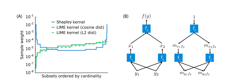
Figure 2: (A) The Shapley kernel weighting is symmetric when all possible $z'$ vectors are ordered by cardinality; there are $2^{15}$ vectors in this example. This is distinctly different from previous heuristically chosen kernels. (B) Compositional models such as deep neural networks are comprised of many simple components. Given analytic solutions for the Shapley values of the components, fast approximations for the full model can be made using DeepLIFT's style of back-propagation.

图 2：（A）当所有可能的 $z'$ 向量按基数排序时，Shapley 核的权重是对称的；本例中有 $2^{15}$ 个向量。这与先前启发式选择的核明显不同。（B）深度网络这类组合模型由许多简单部件构成。如果各部件的 Shapley 值有解析解，就可以用 DeepLIFT 那种反向传播方式，对整个模型做快速近似。

Deep SHAP (DeepLIFT + Shapley values)

While Kernel SHAP can be used on any model, including deep models, it is natural to ask whether there is a way to leverage extra knowledge about the compositional nature of deep networks to improve computational performance. We find an answer to this question through a previously unappreciated connection between Shapley values and DeepLIFT [8]. If we interpret the reference value in Equation 3 as representing $E[x]$ in Equation 12, then DeepLIFT approximates SHAP values assuming that the input features are independent of one another and the deep model is linear. DeepLIFT uses a linear composition rule, which is equivalent to linearizing the non-linear components of a neural network. Its back-propagation rules defining how each component is linearized are intuitive but were heuristically chosen. Since DeepLIFT is an additive feature attribution method that satisfies local accuracy and missingness, we know that Shapley values represent the only attribution values that satisfy consistency. This motivates our adapting DeepLIFT to become a compositional approximation of SHAP values, leading to Deep SHAP.

Deep SHAP（DeepLIFT + Shapley 值）

虽然 Kernel SHAP 可以用于任何模型，包括深度模型，但自然会问：能否利用深度网络具有组合结构这一额外知识，来提高计算效率？我们发现，答案藏在 Shapley 值与 DeepLIFT [8] 之间一条此前未被重视的联系里。如果把方程 3 中的参考值解释为方程 12 中的 $E[x]$，那么 DeepLIFT 就是在假定输入特征相互独立、且深度模型为线性的前提下，对 SHAP 值做近似。DeepLIFT 使用一条线性组合规则，等价于把神经网络中的非线性部件线性化。它用来规定如何线性化各部件的反向传播规则很直观，但却是启发式选定的。既然 DeepLIFT 是满足局部准确和缺失性的可加特征归因方法，我们就知道只有 Shapley 值才是满足一致性的归因。这促使我们把 DeepLIFT 改造成对 SHAP 值的组合近似，从而得到 Deep SHAP。

Deep SHAP combines SHAP values computed for smaller components of the network into SHAP values for the whole network. It does so by recursively passing DeepLIFT’s multipliers, now defined in terms of SHAP values, backwards through the network as in Figure 2B:

Deep SHAP 把为网络中较小部件算出的 SHAP 值组合为整个网络的 SHAP 值。它通过递归地传递 DeepLIFT 的乘数来做到这一点，而这些乘数现在用 SHAP 值来定义，并如图 2B 那样沿网络反向传播：

$$\begin{aligned}
m_{x_j f_3}&=\frac{\phi_i(f_3,x)}{x_j-E[x_j]} \tag{13}\
\forall_{j\in{1,2}}\quad m_{y_i f_j}&=\frac{\phi_i(f_j,y)}{y_i-E[y_i]} \tag{14}\
m_{y_i f_3}&=\sum_{j=1}^{2}m_{y_i f_j}m_{x_j f_3} && \text{chain rule} \tag{15}\
\phi_i(f_3,y)&\approx m_{y_i f_3}(y_i-E[y_i]) && \text{linear approximation} \tag{16}
\end{aligned}$$

$$\begin{aligned}
m_{x_j f_3}&=\frac{\phi_i(f_3,x)}{x_j-E[x_j]} \tag{13}\
\forall_{j\in{1,2}}\quad m_{y_i f_j}&=\frac{\phi_i(f_j,y)}{y_i-E[y_i]} \tag{14}\
m_{y_i f_3}&=\sum_{j=1}^{2}m_{y_i f_j}m_{x_j f_3} && \text{链式法则} \tag{15}\
\phi_i(f_3,y)&\approx m_{y_i f_3}(y_i-E[y_i]) && \text{线性近似} \tag{16}
\end{aligned}$$

Since the SHAP values for the simple network components can be efficiently solved analytically if they are linear, max pooling, or an activation function with just one input, this composition rule enables a fast approximation of values for the whole model. Deep SHAP avoids the need to heuristically choose ways to linearize components. Instead, it derives an effective linearization from the SHAP values computed for each component. The $max$ function offers one example where this leads to improved attributions (see Section 5).

由于当这些简单网络部件是线性的、是最大池化，或是只有一个输入的激活函数时，它们的 SHAP 值可以高效地解析求出，这条组合规则就为整个模型提供了一种快速近似。Deep SHAP 不必再启发式地选择如何把各部件线性化，而是从为每个部件算出的 SHAP 值中导出一种有效的线性化。$max$ 函数就是一个因此得到更好归因的例子（见第 5 节）。

5 Computational and User Study Experiments

5 计算实验与用户研究

We evaluated the benefits of SHAP values using the Kernel SHAP and Deep SHAP approximation methods. First, we compared the computational efficiency and accuracy of Kernel SHAP vs. LIME and Shapley sampling values. Second, we designed user studies to compare SHAP values with alternative feature importance allocations represented by DeepLIFT and LIME. As might be expected, SHAP values prove more consistent with human intuition than other methods that fail to meet Properties 1-3 (Section 2). Finally, we use MNIST digit image classification to compare SHAP with DeepLIFT and LIME.

我们用 Kernel SHAP 和 Deep SHAP 这两种近似方法来评估 SHAP 值的好处。首先，我们比较了 Kernel SHAP 相对于 LIME 和 Shapley 采样值的计算效率与精度。其次，我们设计用户研究，把 SHAP 值与 DeepLIFT 和 LIME 所代表的其他特征重要性分配做比较。正如可以预期的那样，SHAP 值比那些不满足性质 1–3 的方法更符合人类直觉（第 2 节）。最后，我们用 MNIST 数字图像分类，把 SHAP 与 DeepLIFT、LIME 做比较。

5.1 Computational Efficiency

5.1 计算效率

Theorem 2 connects Shapley values from game theory with weighted linear regression. Kernal SHAP uses this connection to compute feature importance. This leads to more accurate estimates with fewer evaluations of the original model than previous sampling-based estimates of Equation 8, particularly when regularization is added to the linear model (Figure 3). Comparing Shapley sampling, SHAP, and LIME on both dense and sparse decision tree models illustrates both the improved sample efficiency of Kernel SHAP and that values from LIME can differ significantly from SHAP values that satisfy local accuracy and consistency.

定理 2 把博弈论中的 Shapley 值与加权线性回归联系起来。Kernel SHAP 利用这一联系来计算特征重要性。与先前基于抽样来估计方程 8 的做法相比，这能在更少的原模型评估次数下得到更准确的估计，尤其是在给线性模型加上正则化时（图 3）。在密集和稀疏的决策树模型上比较 Shapley 采样、SHAP 和 LIME，既说明了 Kernel SHAP 更高的样本效率，也说明 LIME 给出的值可能与满足局部准确和一致性的 SHAP 值相差很大。

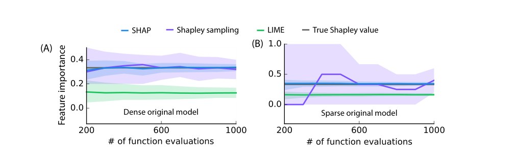
Figure 3: Comparison of three additive feature attribution methods: Kernel SHAP (using a debiased lasso), Shapley sampling values, and LIME (using the open source implementation). Feature importance estimates are shown for one feature in two models as the number of evaluations of the original model function increases. The 10th and 90th percentiles are shown for 200 replicate estimates at each sample size. (A) A decision tree model using all 10 input features is explained for a single input. (B) A decision tree using only 3 of 100 input features is explained for a single input.

图 3：三种可加特征归因方法的比较：Kernel SHAP（使用去偏 lasso）、Shapley 采样值，以及 LIME（使用开源实现）。图中给出两个模型里某一个特征的重要性估计，随对原模型函数评估次数增加而变化。每个样本量上画出 200 次重复估计的第 10 和第 90 百分位。（A）对一个使用全部 10 个输入特征的决策树模型，解释单个输入。（B）对一个只使用 100 个输入特征中 3 个的决策树，解释单个输入。

5.2 Consistency with Human Intuition

5.2 与人类直觉的一致性

Theorem 1 provides a strong incentive for all additive feature attribution methods to use SHAP values. Both LIME and DeepLIFT, as originally demonstrated, compute different feature importance values. To validate the importance of Theorem 1, we compared explanations from LIME, DeepLIFT, and SHAP with user explanations of simple models (using Amazon Mechanical Turk). Our testing assumes that good model explanations should be consistent with explanations from humans who understand that model.

定理 1 为所有可加特征归因方法使用 SHAP 值提供了很强的动机。LIME 和 DeepLIFT 按原先展示的方式，算出的是不同的特征重要性值。为验证定理 1 的重要性，我们把 LIME、DeepLIFT 和 SHAP 的解释，与使用者对简单模型的解释做了比较（使用 Amazon Mechanical Turk）。我们的检验假定：好的模型解释应当与理解该模型的人给出的解释相一致。

We compared LIME, DeepLIFT, and SHAP with human explanations for two settings. The first setting used a sickness score that was higher when only one of two symptoms was present (Figure 4A). The second used a max allocation problem to which DeepLIFT can be applied. Participants were told a short story about how three men made money based on the maximum score any of them achieved (Figure 4B). In both cases, participants were asked to assign credit for the output (the sickness score or money won) among the inputs (i.e., symptoms or players). We found a much stronger agreement between human explanations and SHAP than with other methods. SHAP’s improved performance for max functions addresses the open problem of max pooling functions in DeepLIFT [7].

我们在两种设定下比较了 LIME、DeepLIFT、SHAP 与人的解释。第一种设定使用一种“生病分数”：当两种症状中只有一种出现时，分数反而更高（图 4A）。第二种是可以把 DeepLIFT 用上去的最大值分配问题。被试听到一个短故事：三个男人按他们之中任何人达到的最高分数来赚钱（图 4B）。在两种情形下，被试都被要求把输出（生病分数或赢到的钱）的功劳分配给各个输入（也即症状或参与者）。我们发现，人的解释与 SHAP 的吻合远强于与其他方法的吻合。SHAP 在 max 函数上的改进，也回应了 DeepLIFT 中最大池化函数这一未决问题 [7]。

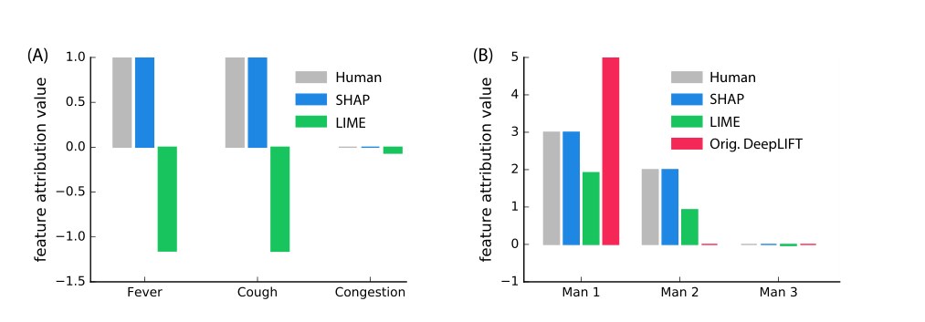
Figure 4: Human feature impact estimates are shown as the most common explanation given among 30 (A) and 52 (B) random individuals, respectively. (A) Feature attributions for a model output value (sickness score) of 2. The model output is 2 when fever and cough are both present, 5 when only one of fever or cough is present, and 0 otherwise. (B) Attributions of profit among three men, given according to the maximum number of questions any man got right. The first man got 5 questions right, the second 4 questions, and the third got none right, so the profit is $5.

图 4：人类对特征影响的估计，分别取 30 人（A）和 52 人（B）中最常见的那种解释。（A）模型输出值（生病分数）为 2 时的特征归因。当发烧和咳嗽同时出现时模型输出为 2，只出现其中之一时为 5，否则为 0。（B）在三人之间分配利润，利润按任何人答对的最多题数给出。第一个人答对 5 题，第二个 4 题，第三个一题未对，因此利润为 5 美元。

5.3 Explaining Class Differences

5.3 解释类别差异

As discussed in Section 4.2, DeepLIFT’s compositional approach suggests a compositional approximation of SHAP values (Deep SHAP). These insights, in turn, improve DeepLIFT, and a new version includes updates to better match Shapley values [7]. Figure 5 extends DeepLIFT’s convolutional network example to highlight the increased performance of estimates that are closer to SHAP values. The pre-trained model and Figure 5 example are the same as those used in [7], with inputs normalized between 0 and 1. Two convolution layers and 2 dense layers are followed by a 10-way softmax output layer. Both DeepLIFT versions explain a normalized version of the linear layer, while SHAP (computed using Kernel SHAP) and LIME explain the model’s output. SHAP and LIME were both run with 50k samples (Supplementary Figure 1); to improve performance, LIME was modified to use single pixel segmentation over the digit pixels. To match [7], we masked 20% of the pixels chosen to switch the predicted class from 8 to 3 according to the feature attribution given by each method.

如第 4.2 节所讨论的，DeepLIFT 的组合思路启示了一种对 SHAP 值的组合近似（Deep SHAP）。这些认识反过来也改进了 DeepLIFT，新版本包含了为更好匹配 Shapley 值而做的更新 [7]。图 5 扩展了 DeepLIFT 的卷积网络例子，以突出更接近 SHAP 值的估计所带来的性能提升。预训练模型和与图 5 相同的例子都来自 [7]，输入被归一化到 0 和 1 之间。两个卷积层和两个全连接层之后是 10 路 softmax 输出层。两个版本的 DeepLIFT 解释的是线性层的一种归一化版本，而 SHAP（用 Kernel SHAP 计算）和 LIME 解释的是模型输出。SHAP 和 LIME 都用了 5 万个样本（补充材料图 1）；为提高表现，LIME 被改成在数字像素上使用单像素分割。为与 [7] 对齐，我们按每种方法给出的特征归因，遮住 20% 被选来把预测类别从 8 改成 3 的像素。

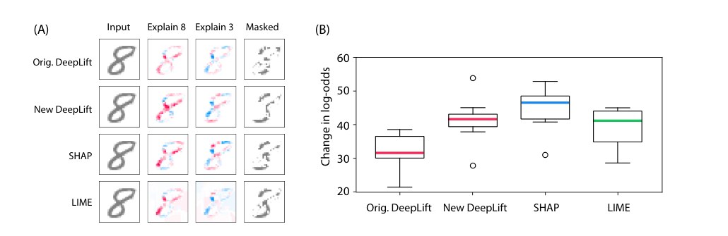
Figure 5: Explaining the output of a convolutional network trained on the MNIST digit dataset. Orig. DeepLIFT has no explicit Shapley approximations, while New DeepLIFT seeks to better approximate Shapley values. (A) Red areas increase the probability of that class, and blue areas decrease the probability. Masked removes pixels in order to go from 8 to 3. (B) The change in log odds when masking over 20 random images supports the use of better estimates of SHAP values.

图 5：解释在 MNIST 数字数据集上训练的卷积网络的输出。原始 DeepLIFT 没有显式的 Shapley 近似，而新的 DeepLIFT 试图更好地逼近 Shapley 值。（A）红色区域提高该类别的概率，蓝色区域降低该概率。Masked 通过去掉像素，把数字从 8 变成 3。（B）在 20 张随机图像上做遮挡时对数几率的变化，支持使用更好的 SHAP 值估计。

6 Conclusion

6 结论

The growing tension between the accuracy and interpretability of model predictions has motivated the development of methods that help users interpret predictions. The SHAP framework identifies the class of additive feature importance methods (which includes six previous methods) and shows there is a unique solution in this class that adheres to desirable properties. The thread of unity that SHAP weaves through the literature is an encouraging sign that common principles about model interpretation can inform the development of future methods.

模型预测在精度与可解释性之间日益增加的张力，推动了帮助使用者解释预测的方法的发展。SHAP 框架识别出可加特征重要性方法这一类（其中包含先前的六种方法），并表明在这类方法中存在唯一满足一组理想性质的解。SHAP 在文献中穿起的这条统一线索是一个令人鼓舞的信号：关于模型解释的共同原则，可以指导未来方法的发展。

We presented several different estimation methods for SHAP values, along with proofs and experiments showing that these values are desirable. Promising next steps involve developing faster model-type-specific estimation methods that make fewer assumptions, integrating work on estimating interaction effects from game theory, and defining new explanation model classes.

我们给出了若干不同的 SHAP 值估计方法，以及说明这些值值得追求的证明和实验。有希望的下一步包括：发展更少依赖假定、更快的面向特定模型类型的估计方法；把博弈论中估计交互效应的工作整合进来；以及定义新的解释模型类。

Acknowledgements

This work was supported by a National Science Foundation (NSF) DBI-135589, NSF CAREER DBI-155230, American Cancer Society 127332-RSG-15-097-01-TBG, National Institute of Health (NIH) AG049196, and NSF Graduate Research Fellowship. We would like to thank Marco Ribeiro, Erik Štrumbelj, Avanti Shrikumar, Yair Zick, the Lee Lab, and the NIPS reviewers for feedback that has significantly improved this work.

本工作得到 National Science Foundation (NSF) DBI-135589、NSF CAREER DBI-155230、American Cancer Society 127332-RSG-15-097-01-TBG、National Institute of Health (NIH) AG049196 以及 NSF Graduate Research Fellowship 的资助。我们感谢 Marco Ribeiro、Erik Štrumbelj、Avanti Shrikumar、Yair Zick、the Lee Lab 以及 NIPS 审稿人提出的反馈，这些意见显著改进了本文。

References

参考文献

[1] Sebastian Bach et al. “On pixel-wise explanations for non-linear classifier decisions by layer-wise relevance propagation” In PloS One 10.7 Public Library of Science, 2015, pp. e0130140

[2] A Charnes, B Golany, M Keane and J Rousseau “Extremal principle solutions of games in characteristic function form: core, Chebychev and Shapley value generalizations” In Econometrics of Planning and Efficiency 11 Springer, 1988, pp. 123–133

[3] Anupam Datta, Shayak Sen and Yair Zick “Algorithmic transparency via quantitative input influence: Theory and experiments with learning systems” In Security and Privacy (SP), 2016 IEEE Symposium on , 2016, pp. 598–617 IEEE

[4] Stan Lipovetsky and Michael Conklin “Analysis of regression in game theory approach” In Applied Stochastic Models in Business and Industry 17.4 Wiley Online Library, 2001, pp. 319–330

[5] Marco Ribeiro, Sameer Singh and Carlos Guestrin “Why should i trust you?: Explaining the predictions of any classifier” In Proceedings of the 22nd ACM SIGKDD International Conference on Knowledge Discovery and Data Mining , 2016, pp. 1135–1144 ACM

[6] Lloyd Shapley “A value for n-person games” In Contributions to the Theory of Games 2.28 , 1953, pp. 307–317

[7] Avanti Shrikumar, Peyton Greenside and Anshul Kundaje “Learning Important Features Through Propagating Activation Differences” In arXiv preprint arXiv:1704.02685 , 2017

[8] Avanti Shrikumar, Peyton Greenside, Anna Shcherbina and Anshul Kundaje “Not Just a Black Box: Learning Important Features Through Propagating Activation Differences” In arXiv preprint arXiv:1605.01713 , 2016

[9] Erik Štrumbelj and Igor Kononenko “Explaining prediction models and individual predictions with feature contributions” In Knowledge and information systems 41.3 Springer, 2014, pp. 647–665

[10] H Young “Monotonic solutions of cooperative games” In International Journal of Game Theory 14.2 Springer, 1985, pp. 65–72