Squeeze-and-Excitation Networks

Jie Hu    Li Shen Thanks:  Jie Hu and Enhua Wu are with the State Key Laboratory of Computer Science, Institute of Software, Chinese Academy of Sciences, Beijing, 100190, China. They are also with the University of Chinese Academy of Sciences, Beijing, 100049, China. Jie Hu is also with Momenta and Enhua Wu is also with the Faculty of Science and Technology & AI Center at University of Macau. E-mail: hujie@ios.ac.cn   ehwu@umac.mo Gang Sun is with LIAMA-NLPR at the Institute of Automation, Chinese Academy of Sciences. He is also with Momenta. E-mail: sungang@momenta.ai Li Shen and Samuel Albanie are with the Visual Geometry Group at the University of Oxford. E-mail: {lishen,albanie}@robots.ox.ac.uk    Samuel Albanie    Gang Sun    Enhua Wu

Abstract

摘要

The central building block of convolutional neural networks (CNNs) is the convolution operator, which enables networks to construct informative features by fusing both spatial and channel-wise information within local receptive fields at each layer. A broad range of prior research has investigated the spatial component of this relationship, seeking to strengthen the representational power of a CNN by enhancing the quality of spatial encodings throughout its feature hierarchy. In this work, we focus instead on the channel relationship and propose a novel architectural unit, which we term the “Squeeze-and-Excitation” (SE) block, that adaptively recalibrates channel-wise feature responses by explicitly modelling interdependencies between channels. We show that these blocks can be stacked together to form SENet architectures that generalise extremely effectively across different datasets. We further demonstrate that SE blocks bring significant improvements in performance for existing state-of-the-art CNNs at slight additional computational cost. Squeeze-and-Excitation Networks formed the foundation of our ILSVRC $2017$ classification submission which won first place and reduced the top-$5$ error to $2.251\%$, surpassing the winning entry of $2016$ by a relative improvement of ${\sim}25\%$. Models and code are available at https://github.com/hujie-frank/SENet.

卷积神经网络（CNN）的核心构件是卷积算子：在每一层的局部感受野内融合空间与通道信息，从而构造有信息量的特征。大量先前工作关注这一关系中的空间分量，试图通过增强特征层级中空间编码的质量来加强 CNN 的表示能力。本文转而关注通道关系，并提出一种称为「Squeeze-and-Excitation」（SE）块的新型结构单元：通过显式建模通道间依赖，自适应地重标定通道维特征响应。我们表明这些块可以堆叠成 SENet 架构，并在不同数据集上极有效地泛化。我们还证明，SE 块能以轻微额外计算代价显著提升现有最优 CNN 的表现。Squeeze-and-Excitation Networks 构成我们 ILSVRC $2017$ 分类提交的基础：该提交获得第一名，并将 top-$5$ 错误率降到 $2.251\%$，相对 $2016$ 年冠军条目相对提升约 ${\sim}25\%$。模型与代码见 https://github.com/hujie-frank/SENet。

I Introduction

I 引言

Index Terms:

Convolutional neural networks (CNNs) have proven to be useful models for tackling a wide range of visual tasks [1, 2, 3, 4]. At each convolutional layer in the network, a collection of filters expresses neighbourhood spatial connectivity patterns along input channels—fusing spatial and channel-wise information together within local receptive fields. By interleaving a series of convolutional layers with non-linear activation functions and downsampling operators, CNNs are able to produce image representations that capture hierarchical patterns and attain global theoretical receptive fields. A central theme of computer vision research is the search for more powerful representations that capture only those properties of an image that are most salient for a given task, enabling improved performance. As a widely-used family of models for vision tasks, the development of new neural network architecture designs now represents a key frontier in this search. Recent research has shown that the representations produced by CNNs can be strengthened by integrating learning mechanisms into the network that help capture spatial correlations between features. One such approach, popularised by the Inception family of architectures [5, 6], incorporates multi-scale processes into network modules to achieve improved performance. Further work has sought to better model spatial dependencies [7, 8] and incorporate spatial attention into the structure of the network [9].

索引词：

卷积神经网络（CNN）已被证明是处理广泛视觉任务的有用模型 [1, 2, 3, 4]。网络中每一卷积层的一组滤波器表达沿输入通道的邻域空间连接模式——在局部感受野内把空间与通道信息融在一起。通过将一系列卷积层与非线性激活、下采样算子交错，CNN 能产生捕捉层次模式、并具有全局理论感受野的图像表示。计算机视觉研究的中心主题之一，是寻找更强的表示，只捕捉对给定任务最显著的图像性质，从而提升表现。作为视觉任务广泛使用的模型族，新神经网络架构设计现已成为这一搜索的关键前沿。近期研究表明，把有助于捕捉特征空间相关的学习机制集成进网络，可以加强 CNN 产生的表示。一类由 Inception 族架构 [5, 6] 推广的做法，是在网络模块中引入多尺度过程以提升表现。后续工作试图更好地建模空间依赖 [7, 8]，并把空间注意力纳入网络结构 [9]。

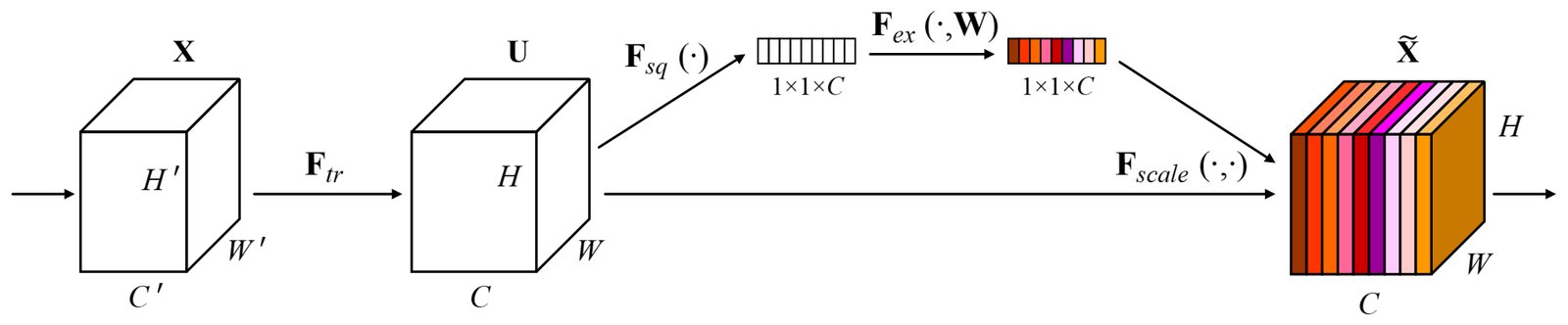
Fig. 1: A Squeeze-and-Excitation block.

图 1：一个 Squeeze-and-Excitation 块。

In this paper, we investigate a different aspect of network design - the relationship between channels. We introduce a new architectural unit, which we term the Squeeze-and-Excitation (SE) block, with the goal of improving the quality of representations produced by a network by explicitly modelling the interdependencies between the channels of its convolutional features. To this end, we propose a mechanism that allows the network to perform feature recalibration, through which it can learn to use global information to selectively emphasise informative features and suppress less useful ones.

本文研究网络设计的另一侧面——通道之间的关系。我们引入称为 Squeeze-and-Excitation（SE）块的新结构单元，目标是通过显式建模卷积特征各通道之间的依赖，提升网络表示质量。为此，我们提出一种允许网络做特征重标定的机制：学习利用全局信息，有选择地强调信息丰富的特征、抑制不太有用的特征。

The structure of the SE building block is depicted in Fig. 1. For any given transformation $\mathbf{F}_{tr}$ mapping the input $\mathbf{X}$ to the feature maps $\mathbf{U}$ where $\mathbf{U}\in\mathbb{R}^{H\times W\times C}$, e.g. a convolution, we can construct a corresponding SE block to perform feature recalibration. The features $\mathbf{U}$ are first passed through a squeeze operation, which produces a channel descriptor by aggregating feature maps across their spatial dimensions ($H\times W$). The function of this descriptor is to produce an embedding of the global distribution of channel-wise feature responses, allowing information from the global receptive field of the network to be used by all its layers. The aggregation is followed by an excitation operation, which takes the form of a simple self-gating mechanism that takes the embedding as input and produces a collection of per-channel modulation weights. These weights are applied to the feature maps $\mathbf{U}$ to generate the output of the SE block which can be fed directly into subsequent layers of the network.

SE 构建块结构见图 1。对任意把输入 $\mathbf{X}$ 映射到特征图 $\mathbf{U}$（$\mathbf{U}\in\mathbb{R}^{H\times W\times C}$）的变换 $\mathbf{F}_{tr}$（例如卷积），可构造对应的 SE 块做特征重标定。特征 $\mathbf{U}$ 先经过 squeeze 操作：沿空间维（$H\times W$）聚合特征图，得到通道描述子。该描述子嵌入通道维特征响应的全局分布，使网络各层都能使用来自全局感受野的信息。聚合之后是 excitation 操作：一种简单的自门控机制，以该嵌入为输入，产生逐通道调制权重。这些权重作用于特征图 $\mathbf{U}$，得到 SE 块输出，可直接送入网络后续层。

It is possible to construct an SE network (SENet) by simply stacking a collection of SE blocks. Moreover, these SE blocks can also be used as a drop-in replacement for the original block at a range of depths in the network architecture (Section VI-D). While the template for the building block is generic, the role it performs at different depths differs throughout the network. In earlier layers, it excites informative features in a class-agnostic manner, strengthening the shared low-level representations. In later layers, the SE blocks become increasingly specialised, and respond to different inputs in a highly class-specific manner (Section VII-B). As a consequence, the benefits of the feature recalibration performed by SE blocks can be accumulated through the network.

通过简单堆叠一组 SE 块即可构造 SE 网络（SENet）。这些 SE 块也可作为即插即用替换，用于网络架构不同深度的原始块（第 VI-D 节）。尽管构建块模板通用，它在不同深度扮演的角色不同。较早层以类别无关方式激发信息丰富的特征，加强共享的低层表示；较后层 SE 块日益特化，并以高度类别相关的方式响应不同输入（第 VII-B 节）。因此，SE 块所做特征重标定的收益可以在网络中累积。

The design and development of new CNN architectures is a difficult engineering task, typically requiring the selection of many new hyperparameters and layer configurations. By contrast, the structure of the SE block is simple and can be used directly in existing state-of-the-art architectures by replacing components with their SE counterparts, where the performance can be effectively enhanced. SE blocks are also computationally lightweight and impose only a slight increase in model complexity and computational burden.

设计开发新 CNN 架构是困难的工程任务，通常需要选择许多新超参与层配置。相对地，SE 块结构简单，可直接用于现有最优架构：用 SE 对应物替换组件即可有效提升表现。SE 块在计算上也轻量，仅轻微增加模型复杂度与计算负担。

To provide evidence for these claims, we develop several SENets and conduct an extensive evaluation on the ImageNet dataset [10]. We also present results beyond ImageNet that indicate that the benefits of our approach are not restricted to a specific dataset or task. By making use of SENets, we ranked first in the ILSVRC 2017 classification competition. Our best model ensemble achieves a $2.251\%$ top-5 error on the test set[^1]. This represents roughly a $25\%$ relative improvement when compared to the winner entry of the previous year (top-5 error of $2.991\%$).

为支撑这些论断，我们开发若干 SENet，并在 ImageNet 数据集 [10] 上做广泛评测。我们也给出超出 ImageNet 的结果，表明方法收益不限于特定数据集或任务。借助 SENet，我们在 ILSVRC 2017 分类竞赛中排名第一。最佳模型集成在测试集上达到 $2.251\%$ 的 top-5 错误率[^1]。相对前一年冠军条目（top-5 错误率 $2.991\%$），这大约是 $25\%$ 的相对提升。

II Related Work

II 相关工作

Deeper architectures. VGGNets [11] and Inception models [5] showed that increasing the depth of a network could significantly increase the quality of representations that it was capable of learning. By regulating the distribution of the inputs to each layer, Batch Normalization (BN) [6] added stability to the learning process in deep networks and produced smoother optimisation surfaces [12]. Building on these works, ResNets demonstrated that it was possible to learn considerably deeper and stronger networks through the use of identity-based skip connections [13, 14]. Highway networks [15] introduced a gating mechanism to regulate the flow of information along shortcut connections. Following these works, there have been further reformulations of the connections between network layers [16, 17], which show promising improvements to the learning and representational properties of deep networks.

更深的架构。 VGGNets [11] 与 Inception 模型 [5] 表明加深网络可显著提升其可学表示的质量。批归一化（BN）[6] 通过调节每层输入分布，为深层网络学习增加稳定性，并产生更平滑的优化曲面 [12]。在此基础上，ResNets 表明借助恒等跳跃连接可以学习显著更深、更强的网络 [13, 14]。Highway 网络 [15] 引入门控机制以调节捷径上的信息流。随后还有对层间连接的进一步改写 [16, 17]，显示对深层网络学习与表示性质有可观改进。

An alternative, but closely related line of research has focused on methods to improve the functional form of the computational elements contained within a network. Grouped convolutions have proven to be a popular approach for increasing the cardinality of learned transformations [18, 19]. More flexible compositions of operators can be achieved with multi-branch convolutions [6, 5, 20, 21], which can be viewed as a natural extension of the grouping operator. In prior work, cross-channel correlations are typically mapped as new combinations of features, either independently of spatial structure [22, 23] or jointly by using standard convolutional filters [24] with $1\times 1$ convolutions. Much of this research has concentrated on the objective of reducing model and computational complexity, reflecting an assumption that channel relationships can be formulated as a composition of instance-agnostic functions with local receptive fields. In contrast, we claim that providing the unit with a mechanism to explicitly model dynamic, non-linear dependencies between channels using global information can ease the learning process, and significantly enhance the representational power of the network.

另一条密切相关的研究线关注改进网络内部计算元件的函数形式。分组卷积已成为增加所学变换基数的流行做法 [18, 19]。多分支卷积 [6, 5, 20, 21] 可实现更灵活的算子组合，可视为分组算子的自然扩展。先前工作中，跨通道相关通常被映射为特征的新组合：或独立于空间结构 [22, 23]，或用标准卷积滤波器（$1\times 1$ 卷积）联合建模 [24]。这类研究多以降低模型与计算复杂度为目标，隐含假设通道关系可表述为具有局部感受野的实例无关函数的复合。相对地，我们主张：为单位提供用全局信息显式建模通道间动态非线性依赖的机制，可减轻学习过程并显著增强网络表示能力。

Algorithmic Architecture Search. Alongside the works described above, there is also a rich history of research that aims to forgo manual architecture design and instead seeks to learn the structure of the network automatically. Much of the early work in this domain was conducted in the neuro-evolution community, which established methods for searching across network topologies with evolutionary methods [25, 26]. While often computationally demanding, evolutionary search has had notable successes which include finding good memory cells for sequence models [27, 28] and learning sophisticated architectures for large-scale image classification [29, 30, 31]. With the goal of reducing the computational burden of these methods, efficient alternatives to this approach have been proposed based on Lamarckian inheritance [32] and differentiable architecture search [33].

算法化架构搜索。 除上述工作外，还有丰富的研究试图放弃手工架构设计，转而自动学习网络结构。该领域早期大量工作在神经演化社区进行，建立了用演化方法搜索网络拓扑的方法 [25, 26]。尽管常计算昂贵，演化搜索有过显著成功，包括为序列模型找到好的记忆单元 [27, 28]，以及为大规模图像分类学习复杂架构 [29, 30, 31]。为降低计算负担，已有基于拉马克遗传 [32] 与可微架构搜索 [33] 的高效替代。

By formulating architecture search as hyperparameter optimisation, random search [34] and other more sophisticated model-based optimisation techniques [35, 36] can also be used to tackle the problem. Topology selection as a path through a fabric of possible designs [37] and direct architecture prediction [38, 39] have been proposed as additional viable architecture search tools. Particularly strong results have been achieved with techniques from reinforcement learning [40, 41, 42, 43, 44]. SE blocks can be used as atomic building blocks for these search algorithms, and were demonstrated to be highly effective in this capacity in concurrent work [45].

把架构搜索表述为超参优化后，随机搜索 [34] 及其他更精细的基于模型的优化技术 [35, 36] 也可用于该问题。把拓扑选择看作穿过可能设计织物的路径 [37]，以及直接架构预测 [38, 39]，也被提出为可行的架构搜索工具。用强化学习的技术取得了特别强的结果 [40, 41, 42, 43, 44]。SE 块可作为这些搜索算法的原子构建块，并在同期工作 [45] 中被证明在这一角色上高度有效。

Attention and gating mechanisms. Attention can be interpreted as a means of biasing the allocation of available computational resources towards the most informative components of a signal [46, 47, 48, 49, 50, 51]. Attention mechanisms have demonstrated their utility across many tasks including sequence learning [52, 53], localisation and understanding in images [54, 9], image captioning [55, 56] and lip reading [57]. In these applications, it can be incorporated as an operator following one or more layers representing higher-level abstractions for adaptation between modalities. Some works provide interesting studies into the combined use of spatial and channel attention [58, 59]. Wang et al. [58] introduced a powerful trunk-and-mask attention mechanism based on hourglass modules [8] that is inserted between the intermediate stages of deep residual networks. By contrast, our proposed SE block comprises a lightweight gating mechanism which focuses on enhancing the representational power of the network by modelling channel-wise relationships in a computationally efficient manner.

注意力与门控机制。 注意力可理解为把可用计算资源偏向信号中最有信息分量的一种手段 [46, 47, 48, 49, 50, 51]。注意力机制已在许多任务上展示效用，包括序列学习 [52, 53]、图像中的定位与理解 [54, 9]、图像描述 [55, 56] 与唇读 [57]。在这些应用中，它可作为跟在一层或多层更高层抽象之后的算子，用于模态间适配。一些工作对空间与通道注意力的联合使用做了有趣研究 [58, 59]。Wang et al. [58] 引入基于沙漏模块 [8] 的强力主干–掩码注意力机制，插入深度残差网络的中间阶段之间。相对地，我们提出的 SE 块是轻量门控机制，专注以计算高效方式建模通道关系，从而增强网络表示能力。

III Squeeze-and-Excitation Blocks

III Squeeze-and-Excitation 块

A Squeeze-and-Excitation block is a computational unit which can be built upon a transformation $\mathbf{F}_{tr}$ mapping an input $\mathbf{X}\in\mathbb{R}^{H^{\prime}\times W^{\prime}\times C^{\prime}}$ to feature maps $\mathbf{U}\in\mathbb{R}^{H\times W\times C}$. In the notation that follows we take $\mathbf{F}_{tr}$ to be a convolutional operator and use $\mathbf{V}=[\mathbf{v}_{1},\mathbf{v}_{2},\dots,\mathbf{v}_{C}]$ to denote the learned set of filter kernels, where $\mathbf{v}_{c}$ refers to the parameters of the $c$-th filter. We can then write the outputs as $\mathbf{U}=[\mathbf{u}_{1},\mathbf{u}_{2},\dots,\mathbf{u}_{C}]$, where

Squeeze-and-Excitation 块是可建立在变换 $\mathbf{F}_{tr}$ 之上的计算单元，该变换把输入 $\mathbf{X}\in\mathbb{R}^{H^{\prime}\times W^{\prime}\times C^{\prime}}$ 映射到特征图 $\mathbf{U}\in\mathbb{R}^{H\times W\times C}$。下文记号中，取 $\mathbf{F}_{tr}$ 为卷积算子，并用 $\mathbf{V}=[\mathbf{v}_{1},\mathbf{v}_{2},\dots,\mathbf{v}_{C}]$ 表示所学滤波器核集合，其中 $\mathbf{v}_{c}$ 为第 $c$ 个滤波器的参数。输出可写为 $\mathbf{U}=[\mathbf{u}_{1},\mathbf{u}_{2},\dots,\mathbf{u}_{C}]$，其中

$$\mathbf{u}_{c}=\mathbf{v}_{c}\ast\mathbf{X}=\sum_{s=1}^{C^{\prime}}\mathbf{v}^{s}_{c}\ast\mathbf{x}^{s}. \tag{1}$$

Here $\ast$ denotes convolution, $\mathbf{v}_{c}=[\mathbf{v}^{1}_{c},\mathbf{v}^{2}_{c},\dots,\mathbf{v}^{C^{\prime}}_{c}]$, $\mathbf{X}=[\mathbf{x}^{1},\mathbf{x}^{2},\dots,\mathbf{x}^{C^{\prime}}]$ and $\mathbf{u}_{c}\in\mathbb{R}^{H\times W}$. $\mathbf{v}^{s}_{c}$ is a $2$D spatial kernel representing a single channel of $\mathbf{v}_{c}$ that acts on the corresponding channel of $\mathbf{X}$. To simplify the notation, bias terms are omitted. Since the output is produced by a summation through all channels, channel dependencies are implicitly embedded in $\mathbf{v}_{c}$, but are entangled with the local spatial correlation captured by the filters. The channel relationships modelled by convolution are inherently implicit and local (except the ones at top-most layers). We expect the learning of convolutional features to be enhanced by explicitly modelling channel interdependencies, so that the network is able to increase its sensitivity to informative features which can be exploited by subsequent transformations. Consequently, we would like to provide it with access to global information and recalibrate filter responses in two steps, squeeze and excitation, before they are fed into the next transformation. A diagram illustrating the structure of an SE block is shown in Fig. 1.

此处 $\ast$ 表示卷积，$\mathbf{v}_{c}=[\mathbf{v}^{1}_{c},\mathbf{v}^{2}_{c},\dots,\mathbf{v}^{C^{\prime}}_{c}]$，$\mathbf{X}=[\mathbf{x}^{1},\mathbf{x}^{2},\dots,\mathbf{x}^{C^{\prime}}]$，$\mathbf{u}_{c}\in\mathbb{R}^{H\times W}$。$\mathbf{v}^{s}_{c}$ 是表示 $\mathbf{v}_{c}$ 单通道的二维空间核，作用于 $\mathbf{X}$ 的对应通道。为简化记号，省略偏置项。由于输出由对所有通道求和得到，通道依赖隐式嵌入在 $\mathbf{v}_{c}$ 中，但与滤波器捕捉的局部空间相关纠缠在一起。卷积所建模的通道关系本质上是隐式且局部的（除最顶层外）。我们期望通过显式建模通道相互依赖来增强卷积特征学习，使网络能提高对后续变换可利用的信息特征的敏感度。因此，我们希望在特征送入下一变换之前，分两步——squeeze 与 excitation——为其提供全局信息并重标定滤波器响应。SE 块结构示意见图 1。

III-A Squeeze: Global Information Embedding

III-A Squeeze：全局信息嵌入

In order to tackle the issue of exploiting channel dependencies, we first consider the signal to each channel in the output features. Each of the learned filters operates with a local receptive field and consequently each unit of the transformation output $\mathbf{U}$ is unable to exploit contextual information outside of this region.

为利用通道依赖，我们首先考虑输出特征中每个通道上的信号。每个所学滤波器以局部感受野运算，因而变换输出 $\mathbf{U}$ 的每个单元无法利用该区域之外的上下文信息。

To mitigate this problem, we propose to squeeze global spatial information into a channel descriptor. This is achieved by using global average pooling to generate channel-wise statistics. Formally, a statistic $\mathbf{z}\in\mathbb{R}^{C}$ is generated by shrinking $\mathbf{U}$ through its spatial dimensions $H\times W$, such that the $c$-th element of $\mathbf{z}$ is calculated by:

为缓解这一问题，我们提出把全局空间信息 squeeze 成通道描述子。做法是用全局平均池化生成通道维统计量。形式化地，统计量 $\mathbf{z}\in\mathbb{R}^{C}$ 通过沿空间维 $H\times W$ 收缩 $\mathbf{U}$ 得到，其第 $c$ 个元素为：

$$z_{c}=\mathbf{F}_{sq}(\mathbf{u}_{c})=\frac{1}{H\times W}\sum_{i=1}^{H}\sum_{j=1}^{W}u_{c}(i,j). \tag{2}$$

Discussion. The output of the transformation $\mathbf{U}$ can be interpreted as a collection of the local descriptors whose statistics are expressive for the whole image. Exploiting such information is prevalent in prior feature engineering work [60, 61, 62]. We opt for the simplest aggregation technique, global average pooling, noting that more sophisticated strategies could be employed here as well.

讨论。 变换输出 $\mathbf{U}$ 可理解为局部描述子的集合，其统计量对整幅图像有表达力。利用这类信息在先前特征工程工作中很常见 [60, 61, 62]。我们选择最简单的聚合技术——全局平均池化，并指出此处也可采用更复杂的策略。

III-B Excitation: Adaptive Recalibration

III-B Excitation：自适应重标定

To make use of the information aggregated in the squeeze operation, we follow it with a second operation which aims to fully capture channel-wise dependencies. To fulfil this objective, the function must meet two criteria: first, it must be flexible (in particular, it must be capable of learning a nonlinear interaction between channels) and second, it must learn a non-mutually-exclusive relationship since we would like to ensure that multiple channels are allowed to be emphasised (rather than enforcing a one-hot activation). To meet these criteria, we opt to employ a simple gating mechanism with a sigmoid activation:

为利用 squeeze 操作聚合的信息，我们紧接第二步操作，旨在充分捕捉通道维依赖。为实现该目标，函数须满足两条：第一，必须灵活（尤其须能学习通道间非线性交互）；第二，必须学习非互斥关系，因为我们希望允许多个通道同时被强调（而非强制独热激活）。为满足这些条件，我们采用带 sigmoid 激活的简单门控机制：

$$\mathbf{s}=\mathbf{F}_{ex}(\mathbf{z},\mathbf{W})=\sigma(g(\mathbf{z},\mathbf{W}))=\sigma(\mathbf{W}_{2}\delta(\mathbf{W}_{1}\mathbf{z})), \tag{3}$$

where $\delta$ refers to the ReLU [63] function, $\mathbf{W}_{1}\in\mathbb{R}^{\frac{C}{r}\times C}$ and $\mathbf{W}_{2}\in\mathbb{R}^{C\times\frac{C}{r}}$. To limit model complexity and aid generalisation, we parameterise the gating mechanism by forming a bottleneck with two fully-connected (FC) layers around the non-linearity, i.e. a dimensionality-reduction layer with reduction ratio $r$ (this parameter choice is discussed in Section VI-A), a ReLU and then a dimensionality-increasing layer returning to the channel dimension of the transformation output $\mathbf{U}$. The final output of the block is obtained by rescaling $\mathbf{U}$ with the activations $\mathbf{s}$:

其中 $\delta$ 指 ReLU [63] 函数，$\mathbf{W}_{1}\in\mathbb{R}^{\frac{C}{r}\times C}$，$\mathbf{W}_{2}\in\mathbb{R}^{C\times\frac{C}{r}}$。为限制模型复杂度并有助于泛化，我们用非线性两侧的两个全连接（FC）层构成瓶颈来参数化门控：即降维比为 $r$ 的降维层（该参数选择见第 VI-A 节）、ReLU，再是升维回到变换输出 $\mathbf{U}$ 通道维的层。块的最终输出通过对 $\mathbf{U}$ 用激活 $\mathbf{s}$ 重缩放得到：

$$\widetilde{\mathbf{x}}_{c}=\mathbf{F}_{scale}(\mathbf{u}_{c},s_{c})=s_{c}\,\mathbf{u}_{c}, \tag{4}$$

where $\widetilde{\mathbf{X}}=[\widetilde{\mathbf{x}}_{1},\widetilde{\mathbf{x}}_{2},\dots,\widetilde{\mathbf{x}}_{C}]$ and $\mathbf{F}_{scale}(\mathbf{u}_{c},s_{c})$ refers to channel-wise multiplication between the scalar $s_{c}$ and the feature map $\mathbf{u}_{c}\in\mathbb{R}^{H\times W}$.

其中 $\widetilde{\mathbf{X}}=[\widetilde{\mathbf{x}}_{1},\widetilde{\mathbf{x}}_{2},\dots,\widetilde{\mathbf{x}}_{C}]$，$\mathbf{F}_{scale}(\mathbf{u}_{c},s_{c})$ 指标量 $s_{c}$ 与特征图 $\mathbf{u}_{c}\in\mathbb{R}^{H\times W}$ 的通道维乘法。

Discussion. The excitation operator maps the input-specific descriptor $\mathbf{z}$ to a set of channel weights. In this regard, SE blocks intrinsically introduce dynamics conditioned on the input, which can be regarded as a self-attention function on channels whose relationships are not confined to the local receptive field the convolutional filters are responsive to.

讨论。 excitation 算子把输入特定的描述子 $\mathbf{z}$ 映射为一组通道权重。就此而言，SE 块内在地引入以输入为条件的动态，可视为对通道的自注意力函数，其关系不受卷积滤波器所响应的局部感受野限制。

III-C Instantiations

III-C 实例化

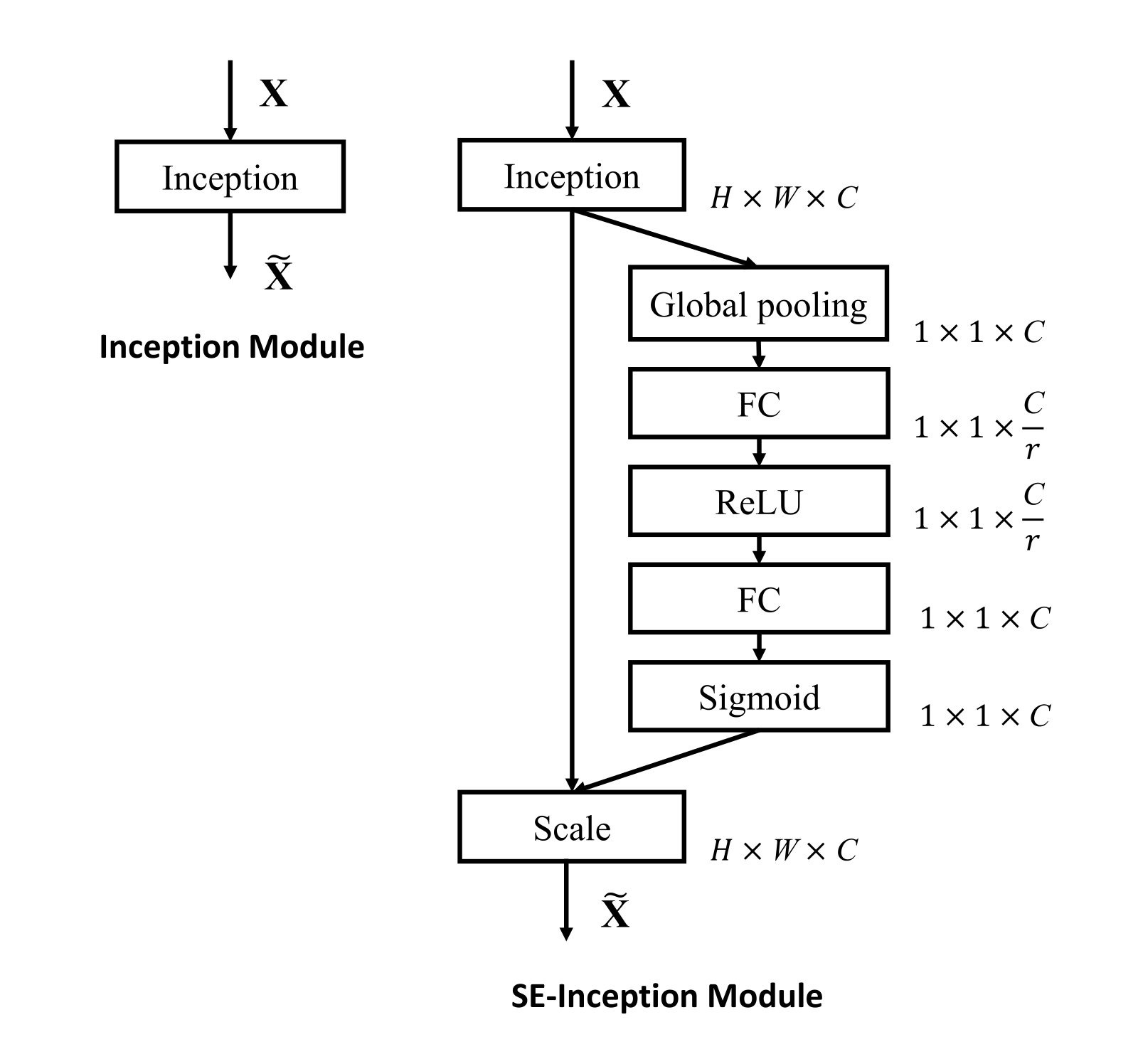
Fig. 2: The schema of the original Inception module (left) and the SE-Inception module (right).

图 2：原始 Inception 模块（左）与 SE-Inception 模块（右）示意。

The SE block can be integrated into standard architectures such as VGGNet [11] by insertion after the non-linearity following each convolution. Moreover, the flexibility of the SE block means that it can be directly applied to transformations beyond standard convolutions. To illustrate this point, we develop SENets by incorporating SE blocks into several examples of more complex architectures, described next.

SE 块可通过在每次卷积后的非线性之后插入，集成到 VGGNet [11] 等标准架构。此外，SE 块的灵活性意味着它可直接用于标准卷积之外的变换。为说明这一点，我们把 SE 块并入若干更复杂架构的例子以构造 SENet，见下文。

We first consider the construction of SE blocks for Inception networks [5]. Here, we simply take the transformation $\mathbf{F}_{tr}$ to be an entire Inception module (see Fig. 2) and by making this change for each such module in the architecture, we obtain an SE-Inception network. SE blocks can also be used directly with residual networks (Fig. 3 depicts the schema of an SE-ResNet module). Here, the SE block transformation $\mathbf{F}_{tr}$ is taken to be the non-identity branch of a residual module. Squeeze and Excitation both act before summation with the identity branch. Further variants that integrate SE blocks with ResNeXt [19], Inception-ResNet [21], MobileNet [64] and ShuffleNet [65] can be constructed by following similar schemes. For concrete examples of SENet architectures, a detailed description of SE-ResNet-50 and SE-ResNeXt-50 is given in Table I.

我们首先考虑为 Inception 网络 [5] 构造 SE 块。这里简单取变换 $\mathbf{F}_{tr}$ 为整个 Inception 模块（见图 2），并对架构中每个此类模块做这一改动，得到 SE-Inception 网络。SE 块也可直接用于残差网络（图 3 给出 SE-ResNet 模块示意）。此处 SE 块变换 $\mathbf{F}_{tr}$ 取为残差模块的非恒等分支。Squeeze 与 Excitation 都在与恒等分支相加之前作用。按类似方案，可进一步构造与 ResNeXt [19]、Inception-ResNet [21]、MobileNet [64] 与 ShuffleNet [65] 集成的变体。SENet 架构的具体例子见表 I 中对 SE-ResNet-50 与 SE-ResNeXt-50 的详细描述。

One consequence of the flexible nature of the SE block is that there are several viable ways in which it could be integrated into these architectures. Therefore, to assess sensitivity to the integration strategy used to incorporate SE blocks into a network architecture, we also provide ablation experiments exploring different designs for block inclusion in Section VI-E.

SE 块灵活性的一个后果是：有多种可行方式把它集成进这些架构。因此，为评估对用于把 SE 块纳入网络架构的集成策略的敏感性，我们还在第 VI-E 节提供探索不同块纳入设计的消融实验。

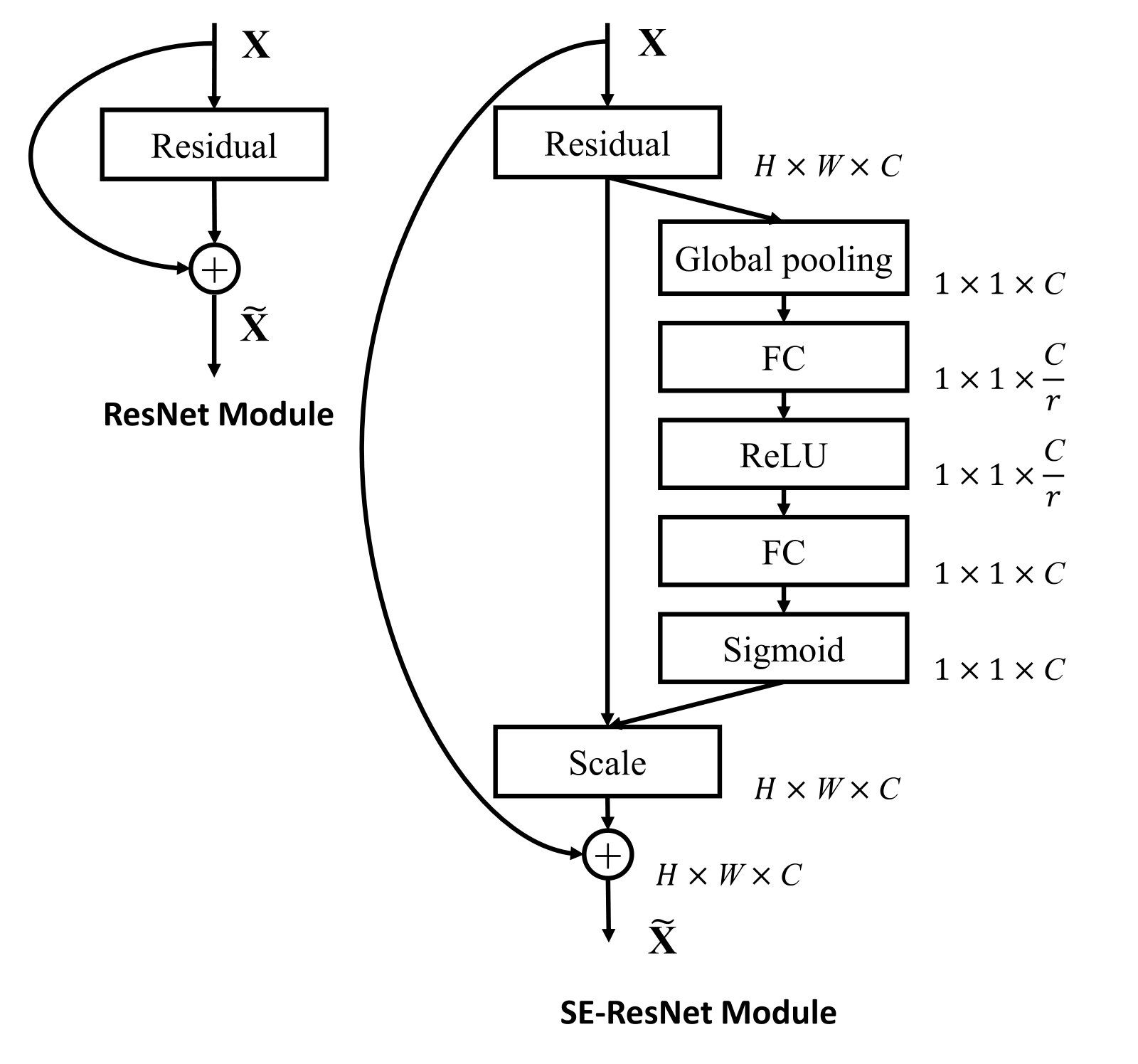
Fig. 3: The schema of the original Residual module (left) and the SE-ResNet module (right).

图 3：原始残差模块（左）与 SE-ResNet 模块（右）示意。

IV Model and Computational Complexity

IV 模型与计算复杂度

For the proposed SE block design to be of practical use, it must offer a good trade-off between improved performance and increased model complexity. To illustrate the computational burden associated with the module, we consider a comparison between ResNet-50 and SE-ResNet-50 as an example. ResNet-50 requires ${\sim}3.86$ GFLOPs in a single forward pass for a $224\times 224$ pixel input image. Each SE block makes use of a global average pooling operation in the squeeze phase and two small FC layers in the excitation phase, followed by an inexpensive channel-wise scaling operation. In the aggregate, when setting the reduction ratio $r$ (introduced in Section III-B) to $16$, SE-ResNet-50 requires ${\sim}3.87$ GFLOPs, corresponding to a $0.26\%$ relative increase over the original ResNet-50. In exchange for this slight additional computational burden, the accuracy of SE-ResNet-50 surpasses that of ResNet-50 and indeed, approaches that of a deeper ResNet-101 network requiring ${\sim}7.58$ GFLOPs (Table II).

要使提出的 SE 块设计具有实用价值，须在提升表现与增加模型复杂度之间取得良好折中。为说明该模块的计算负担，我们以 ResNet-50 与 SE-ResNet-50 的对比为例。对 $224\times 224$ 像素输入图像，ResNet-50 单次前向约需 ${\sim}3.86$ GFLOPs。每个 SE 块在 squeeze 阶段使用全局平均池化，在 excitation 阶段使用两个小型 FC 层，再跟一次廉价的通道维缩放。总体而言，当降维比 $r$（第 III-B 节引入）设为 $16$ 时，SE-ResNet-50 约需 ${\sim}3.87$ GFLOPs，相对原始 ResNet-50 仅增加 $0.26\%$。换取这轻微额外计算负担后，SE-ResNet-50 的准确率超过 ResNet-50，并接近需要 ${\sim}7.58$ GFLOPs 的更深 ResNet-101（表 II）。

In practical terms, a single pass forwards and backwards through ResNet-50 takes $190$ ms, compared to $209$ ms for SE-ResNet-50 with a training minibatch of $256$ images (both timings are performed on a server with $8$ NVIDIA Titan X GPUs). We suggest that this represents a reasonable runtime overhead, which may be further reduced as global pooling and small inner-product operations receive further optimisation in popular GPU libraries. Due to its importance for embedded device applications, we further benchmark CPU inference time for each model: for a $224\times 224$ pixel input image, ResNet-50 takes $164$ ms in comparison to $167$ ms for SE-ResNet-50. We believe that the small additional computational cost incurred by the SE block is justified by its contribution to model performance.

实践中，在训练 minibatch 为 $256$ 张图像时，单次前向加反向穿过 ResNet-50 约需 $190$ ms，SE-ResNet-50 约需 $209$ ms（计时均在配备 $8$ 块 NVIDIA Titan X GPU 的服务器上）。我们认为这是合理的运行时开销，随着流行 GPU 库对全局池化与小型内积运算进一步优化，还可继续降低。鉴于对嵌入式设备应用的重要性，我们还基准了各模型的 CPU 推理时间：对 $224\times 224$ 输入，ResNet-50 需 $164$ ms，SE-ResNet-50 需 $167$ ms。我们相信 SE 块带来的少量额外计算成本，由其对照表现的贡献所正当化。

Output size	ResNet-50	SE-ResNet-50	SE-ResNeXt-50 ($32\times 4$d)
$112\times 112$	conv, $7\times 7$, $64$, stride $2$
$56\times 56$	max pool, $3\times 3$, stride $2$
$\begin{bmatrix}[l]{\rm conv},1\times 1,64\\ {\rm conv},3\times 3,64\\ {\rm conv},1\times 1,256\end{bmatrix}\times 3$	$\begin{bmatrix}[l]{\rm conv},1\times 1,64\\ {\rm conv},3\times 3,64\\ {\rm conv},1\times 1,256\\ fc,[16,256]\end{bmatrix}\times 3$	$\begin{bmatrix}[l]{\rm conv},1\times 1,128\\ {\rm conv},3\times 3,128&C=32\\ {\rm conv},1\times 1,256\\ fc,[16,256]\end{bmatrix}\times 3$
$28\times 28$	$\begin{bmatrix}[l]{\rm conv},1\times 1,128\\ {\rm conv},3\times 3,128\\ {\rm conv},1\times 1,512\end{bmatrix}\times 4$	$\begin{bmatrix}[l]{\rm conv},1\times 1,128\\ {\rm conv},3\times 3,128\\ {\rm conv},1\times 1,512\\ fc,[32,512]\end{bmatrix}\times 4$	$\begin{bmatrix}[l]{\rm conv},1\times 1,256&\\ {\rm conv},3\times 3,256&C=32\\ {\rm conv},1\times 1,512\\ fc,[32,512]\end{bmatrix}\times 4$
$14\times 14$	$\begin{bmatrix}[l]{\rm conv},1\times 1,256\\ {\rm conv},3\times 3,256\\ {\rm conv},1\times 1,1024\end{bmatrix}\times 6$	$\begin{bmatrix}[l]{\rm conv},1\times 1,256\\ {\rm conv},3\times 3,256\\ {\rm conv},1\times 1,1024\\ fc,[64,1024]\end{bmatrix}\times 6$	$\begin{bmatrix}[l]{\rm conv},1\times 1,512&\\ {\rm conv},3\times 3,512&C=32\\ {\rm conv},1\times 1,1024\\ fc,[64,1024]\end{bmatrix}\times 6$
7$\times$7	$\begin{bmatrix}[l]{\rm conv},1\times 1,512\\ {\rm conv},3\times 3,512\\ {\rm conv},1\times 1,2048\end{bmatrix}\times 3$	$\begin{bmatrix}[l]{\rm conv},1\times 1,512\\ {\rm conv},3\times 3,512\\ {\rm conv},1\times 1,2048\\ fc,[128,2048]\end{bmatrix}\times 3$	$\begin{bmatrix}[l]{\rm conv},1\times 1,1024&\\ {\rm conv},3\times 3,1024&C=32\\ {\rm conv},1\times 1,2048\\ fc,[128,2048]\end{bmatrix}\times 3$
$1\times 1$	global average pool, $1000$-d $fc$, softmax

TABLE I: (Left) ResNet-50 [13]. (Middle) SE-ResNet-50. (Right) SE-ResNeXt-50 with a 32$\times$4d template. The shapes and operations with specific parameter settings of a residual building block are listed inside the brackets and the number of stacked blocks in a stage is presented outside. The inner brackets following by fc indicates the output dimension of the two fully connected layers in an SE module.

Output size	ResNet-50	SE-ResNet-50	SE-ResNeXt-50 ($32\times 4$d)
$112\times 112$	conv, $7\times 7$, $64$, stride $2$
$56\times 56$	max pool, $3\times 3$, stride $2$
$\begin{bmatrix}[l]{\rm conv},1\times 1,64\\ {\rm conv},3\times 3,64\\ {\rm conv},1\times 1,256\end{bmatrix}\times 3$	$\begin{bmatrix}[l]{\rm conv},1\times 1,64\\ {\rm conv},3\times 3,64\\ {\rm conv},1\times 1,256\\ fc,[16,256]\end{bmatrix}\times 3$	$\begin{bmatrix}[l]{\rm conv},1\times 1,128\\ {\rm conv},3\times 3,128&C=32\\ {\rm conv},1\times 1,256\\ fc,[16,256]\end{bmatrix}\times 3$
$28\times 28$	$\begin{bmatrix}[l]{\rm conv},1\times 1,128\\ {\rm conv},3\times 3,128\\ {\rm conv},1\times 1,512\end{bmatrix}\times 4$	$\begin{bmatrix}[l]{\rm conv},1\times 1,128\\ {\rm conv},3\times 3,128\\ {\rm conv},1\times 1,512\\ fc,[32,512]\end{bmatrix}\times 4$	$\begin{bmatrix}[l]{\rm conv},1\times 1,256&\\ {\rm conv},3\times 3,256&C=32\\ {\rm conv},1\times 1,512\\ fc,[32,512]\end{bmatrix}\times 4$
$14\times 14$	$\begin{bmatrix}[l]{\rm conv},1\times 1,256\\ {\rm conv},3\times 3,256\\ {\rm conv},1\times 1,1024\end{bmatrix}\times 6$	$\begin{bmatrix}[l]{\rm conv},1\times 1,256\\ {\rm conv},3\times 3,256\\ {\rm conv},1\times 1,1024\\ fc,[64,1024]\end{bmatrix}\times 6$	$\begin{bmatrix}[l]{\rm conv},1\times 1,512&\\ {\rm conv},3\times 3,512&C=32\\ {\rm conv},1\times 1,1024\\ fc,[64,1024]\end{bmatrix}\times 6$
7$\times$7	$\begin{bmatrix}[l]{\rm conv},1\times 1,512\\ {\rm conv},3\times 3,512\\ {\rm conv},1\times 1,2048\end{bmatrix}\times 3$	$\begin{bmatrix}[l]{\rm conv},1\times 1,512\\ {\rm conv},3\times 3,512\\ {\rm conv},1\times 1,2048\\ fc,[128,2048]\end{bmatrix}\times 3$	$\begin{bmatrix}[l]{\rm conv},1\times 1,1024&\\ {\rm conv},3\times 3,1024&C=32\\ {\rm conv},1\times 1,2048\\ fc,[128,2048]\end{bmatrix}\times 3$
$1\times 1$	global average pool, $1000$-d $fc$, softmax

表 I： （左）ResNet-50 [13]。（中）SE-ResNet-50。（右）带 32$\times$4d 模板的 SE-ResNeXt-50。括号内列出残差构建块的形状与带具体参数设定的操作，阶段外数字为堆叠块数。fc 后的内括号表示 SE 模块中两个全连接层的输出维。

	original	re-implementation	SENet
top-1 err.	top-1 err.	top-5 err.	top-5 err.	top-1 err.	top-1 err.	top-5 err.	top-5 err.	GFLOPs	GFLOPs	top-1 err.	top-1 err.	top-5 err.	top-5 err.	GFLOPs	GFLOPs
top-1 err.
top-5 err.
top-1 err.
top-5 err.
GFLOPs
top-1 err.
top-5 err.
GFLOPs
ResNet-50 [13]	$24.7$	$7.8$	$24.80$	$7.48$	$3.86$	$23.29_{(1.51)}$	$6.62_{(0.86)}$	$3.87$
ResNet-101 [13]	$23.6$	$7.1$	$23.17$	$6.52$	$7.58$	$22.38_{(0.79)}$	$6.07_{(0.45)}$	$7.60$
ResNet-152 [13]	$23.0$	$6.7$	$22.42$	$6.34$	$11.30$	$21.57_{(0.85)}$	$5.73_{(0.61)}$	$11.32$
ResNeXt-50 [19]	$22.2$	-	$22.11$	$5.90$	$4.24$	$21.10_{(1.01)}$	$5.49_{(0.41)}$	$4.25$
ResNeXt-101 [19]	$21.2$	$5.6$	$21.18$	$5.57$	$7.99$	$20.70_{(0.48)}$	$5.01_{(0.56)}$	$8.00$
VGG-16 [11]	-	-	$27.02$	$8.81$	$15.47$	$25.22_{(1.80)}$	$7.70_{(1.11)}$	$15.48$
BN-Inception [6]	$25.2$	$7.82$	$25.38$	$7.89$	$2.03$	$24.23_{(1.15)}$	$7.14_{(0.75)}$	$2.04$
Inception-ResNet-v2 [21]	$19.9^{\dagger}$	$4.9^{\dagger}$	$20.37$	$5.21$	$11.75$	$19.80_{(0.57)}$	$4.79_{(0.42)}$	$11.76$

top-1 err.

top-5 err.

top-1 err.

top-5 err.

GFLOPs

top-1 err.

top-5 err.

GFLOPs

TABLE II: Single-crop error rates (%) on the ImageNet validation set and complexity comparisons. The original column refers to the results reported in the original papers (the results of ResNets are obtained from the website: https://github.com/Kaiminghe/deep-residual-networks). To enable a fair comparison, we re-train the baseline models and report the scores in the re-implementation column. The SENet column refers to the corresponding architectures in which SE blocks have been added. The numbers in brackets denote the performance improvement over the re-implemented baselines. $\dagger$ indicates that the model has been evaluated on the non-blacklisted subset of the validation set (this is discussed in more detail in [21]), which may slightly improve results. VGG-16 and SE-VGG-16 are trained with batch normalization.

	original	re-implementation	SENet
top-1 err.	top-1 err.	top-5 err.	top-5 err.	top-1 err.	top-1 err.	top-5 err.	top-5 err.	GFLOPs	GFLOPs	top-1 err.	top-1 err.	top-5 err.	top-5 err.	GFLOPs	GFLOPs
top-1 err.
top-1 err.
top-1 err.
ResNet-50 [13]	$24.7$	$7.8$	$24.80$	$7.48$	$3.86$	$23.29_{(1.51)}$	$6.62_{(0.86)}$	$3.87$
ResNet-101 [13]	$23.6$	$7.1$	$23.17$	$6.52$	$7.58$	$22.38_{(0.79)}$	$6.07_{(0.45)}$	$7.60$
ResNet-152 [13]	$23.0$	$6.7$	$22.42$	$6.34$	$11.30$	$21.57_{(0.85)}$	$5.73_{(0.61)}$	$11.32$
ResNeXt-50 [19]	$22.2$	-	$22.11$	$5.90$	$4.24$	$21.10_{(1.01)}$	$5.49_{(0.41)}$	$4.25$
ResNeXt-101 [19]	$21.2$	$5.6$	$21.18$	$5.57$	$7.99$	$20.70_{(0.48)}$	$5.01_{(0.56)}$	$8.00$
VGG-16 [11]	-	-	$27.02$	$8.81$	$15.47$	$25.22_{(1.80)}$	$7.70_{(1.11)}$	$15.48$
BN-Inception [6]	$25.2$	$7.82$	$25.38$	$7.89$	$2.03$	$24.23_{(1.15)}$	$7.14_{(0.75)}$	$2.04$
Inception-ResNet-v2 [21]	$19.9^{\dagger}$	$4.9^{\dagger}$	$20.37$	$5.21$	$11.75$	$19.80_{(0.57)}$	$4.79_{(0.42)}$	$11.76$
TABLE II: Single-crop error rates (%) on the ImageNet validation set and complexity comparisons. The original column refers to the results reported in the original papers (the results of ResNets are obtained from the website: https://github.com/Kaiminghe/deep-residual-networks). To enable a fair comparison, we re-train the baseline models and report the scores in the re-implementation column. The SENet column refers to the corresponding architectures in which SE blocks have been added. The numbers in brackets denote the performance improvement over the re-implemented baselines. $\dagger$ indicates that the model has been evaluated on the non-blacklisted subset of the validation set (this is discussed in more detail in [21]), which may slightly improve results. VGG-16 and SE-VGG-16 are trained with batch normalization.

表 II：ImageNet 验证集单裁剪错误率（%）与复杂度比较。original 列为原文报告结果（ResNet 结果来自 https://github.com/Kaiminghe/deep-residual-networks）。为公平对比，我们重训基线并在 re-implementation 列报告。SENet 列为加入 SE 块后的对应架构。括号内数字表示相对重实现基线的提升。$\dagger$ 表示在验证集非黑名单子集上评测（详见 [21]），可能略微提升结果。VGG-16 与 SE-VGG-16 带批归一化训练。

We next consider the additional parameters introduced by the proposed SE block. These additional parameters result solely from the two FC layers of the gating mechanism and therefore constitute a small fraction of the total network capacity. Concretely, the total number introduced by the weight parameters of these FC layers is given by:

接下来考虑提出的 SE 块引入的额外参数。这些额外参数仅来自门控机制的两个 FC 层，因此只占总网络容量的一小部分。具体地，这些 FC 层权重参数引入的总量为：

$$\frac{2}{r}\sum_{s=1}^{S}N_{s}\cdot{C_{s}}^{2}, \tag{5}$$

where $r$ denotes the reduction ratio, $S$ refers to the number of stages (a stage refers to the collection of blocks operating on feature maps of a common spatial dimension), $C_{s}$ denotes the dimension of the output channels and $N_{s}$ denotes the number of repeated blocks for stage $s$ (when bias terms are used in FC layers, the introduced parameters and computational cost are typically negligible). SE-ResNet-50 introduces ${\sim}2.5$ million additional parameters beyond the ${\sim}25$ million parameters required by ResNet-50, corresponding to a ${\sim}10\%$ increase. In practice, the majority of these parameters come from the final stage of the network, where the excitation operation is performed across the greatest number of channels. However, we found that this comparatively costly final stage of SE blocks could be removed at only a small cost in performance (${<}0.1\%$ top-$5$ error on ImageNet) reducing the relative parameter increase to ${\sim}4\%$, which may prove useful in cases where parameter usage is a key consideration (see Section VI-D and VII-B for further discussion).

其中 $r$ 为降维比，$S$ 为阶段数（阶段指在共同空间尺寸的特征图上运算的块集合），$C_{s}$ 为输出通道维，$N_{s}$ 为阶段 $s$ 的重复块数（FC 层使用偏置时，引入的参数与计算代价通常可忽略）。SE-ResNet-50 在 ResNet-50 所需约 ${\sim}25$ 百万参数之外额外引入约 ${\sim}2.5$ 百万参数，相对增加约 ${\sim}10\%$。实践中，这些参数多数来自网络最后阶段，因为 excitation 在通道数最多处执行。但我们发现，去掉这一相对昂贵的最后阶段 SE 块，表现代价很小（ImageNet 上 top-$5$ 错误率增加 ${<}0.1\%$），相对参数增幅可降到约 ${\sim}4\%$，在参数用量是关键考量时可能有用（进一步讨论见第 VI-D 与 VII-B 节）。

V Experiments

V 实验

In this section, we conduct experiments to investigate the effectiveness of SE blocks across a range of tasks, datasets and model architectures.

本节通过实验，在一系列任务、数据集与模型架构上考察 SE 块的有效性。

	original	re-implementation	SENet
top-1 err.	top-5 err.	top-5 err.	top-1 err.	top-1 err.	top-5 err.	top-5 err.	MFLOPs	Params	Params	top-1 err.	top-1 err.	top-5 err.	top-5 err.	MFLOPs	Params	Params
top-5 err.
top-1 err.
top-5 err.
Params
top-1 err.
top-5 err.
Params
MobileNet [64]	$29.4$	-	$28.4$	$9.4$	$569$	$4.2$M	$25.3_{(3.1)}$	$7.7_{(1.7)}$	$572$	$4.7$M
ShuffleNet [65]	$32.6$	-	$32.6$	$12.5$	$140$	$1.8$M	$31.0_{(1.6)}$	$11.1_{(1.4)}$	$142$	$2.4$M

top-5 err.

top-1 err.

top-5 err.

Params

top-1 err.

top-5 err.

Params

TABLE III: Single-crop error rates (%) on the ImageNet validation set and complexity comparisons. MobileNet refers to “1.0 MobileNet-224” in [64] and ShuffleNet refers to “ShuffleNet $1\times(g=3)$” in [65]. The numbers in brackets denote the performance improvement over the re-implementation.

	original	re-implementation	SENet
top-1 err.	top-5 err.	top-5 err.	top-1 err.	top-1 err.	top-5 err.	top-5 err.	MFLOPs	Params	Params	top-1 err.	top-1 err.	top-5 err.	top-5 err.	MFLOPs	Params	Params
top-1 err.
Params
top-1 err.
Params
MobileNet [64]	$29.4$	-	$28.4$	$9.4$	$569$	$4.2$M	$25.3_{(3.1)}$	$7.7_{(1.7)}$	$572$	$4.7$M
ShuffleNet [65]	$32.6$	-	$32.6$	$12.5$	$140$	$1.8$M	$31.0_{(1.6)}$	$11.1_{(1.4)}$	$142$	$2.4$M
TABLE III: Single-crop error rates (%) on the ImageNet validation set and complexity comparisons. MobileNet refers to “1.0 MobileNet-224” in [64] and ShuffleNet refers to “ShuffleNet $1\times(g=3)$” in [65]. The numbers in brackets denote the performance improvement over the re-implementation.

表 III：ImageNet 验证集单裁剪错误率（%）与复杂度比较。MobileNet 指 [64] 中的 “1.0 MobileNet-224”，ShuffleNet 指 [65] 中的 “ShuffleNet $1\times(g=3)$”。括号内数字表示相对重实现的提升。

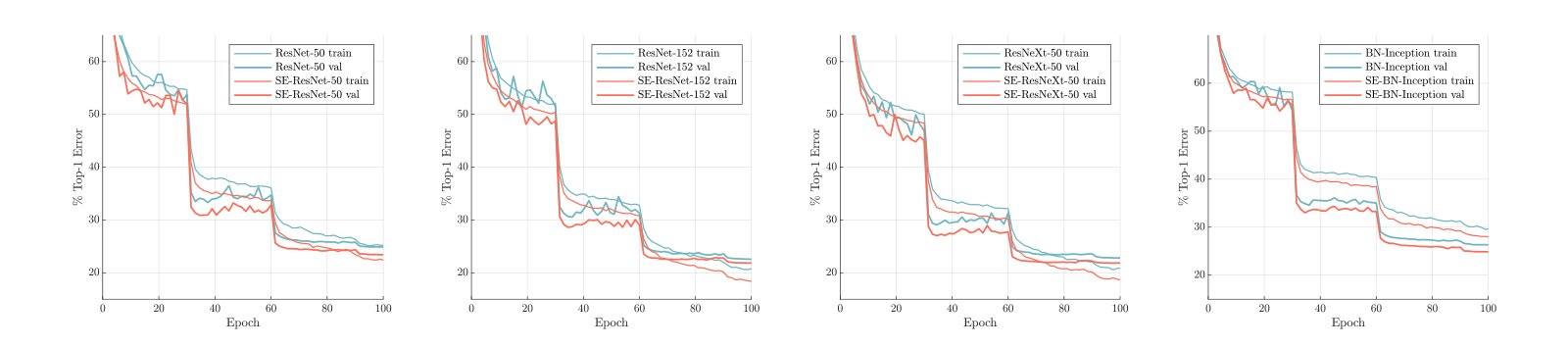
Fig. 4: Training baseline architectures and their SENet counterparts on ImageNet. SENets exhibit improved optimisation characteristics and produce consistent gains in performance which are sustained throughout the training process.

图 4：在 ImageNet 上训练基线架构及其 SENet 对应物。SENet 表现出更好的优化特性，并在整个训练过程中持续产生稳定的表现增益。

V-A Image Classification

V-A 图像分类

To evaluate the influence of SE blocks, we first perform experiments on the ImageNet $2012$ dataset [10] which comprises $1.28$ million training images and $50$K validation images from $1000$ different classes. We train networks on the training set and report the top-$1$ and top-$5$ error on the validation set.

为评估 SE 块的影响，我们首先在 ImageNet $2012$ 数据集 [10] 上实验：该数据集含 $1.28$ 百万训练图像与来自 $1000$ 个不同类别的 $50$K 验证图像。我们在训练集上训练网络，并在验证集上报告 top-$1$ 与 top-$5$ 错误率。

Each baseline network architecture and its corresponding SE counterpart are trained with identical optimisation schemes. We follow standard practices and perform data augmentation with random cropping using scale and aspect ratio [5] to a size of $224\times 224$ pixels (or $299\times 299$ for Inception-ResNet-v2 [21] and SE-Inception-ResNet-v2) and perform random horizontal flipping. Each input image is normalised through mean RGB-channel subtraction. All models are trained on our distributed learning system ROCS which is designed to handle efficient parallel training of large networks. Optimisation is performed using synchronous SGD with momentum $0.9$ and a minibatch size of $1024$. The initial learning rate is set to $0.6$ and decreased by a factor of $10$ every $30$ epochs. Models are trained for $100$ epochs from scratch, using the weight initialisation strategy described in [66]. The reduction ratio $r$ (in Section III-B) is set to $16$ by default (except where stated otherwise).

每个基线网络架构及其对应 SE 版本使用相同优化方案训练。我们遵循标准做法，用尺度与长宽比随机裁剪 [5] 做数据增强到 $224\times 224$ 像素（Inception-ResNet-v2 [21] 与 SE-Inception-ResNet-v2 为 $299\times 299$），并做随机水平翻转。每张输入图像经均值 RGB 通道减法归一化。所有模型在我们设计用于高效并行训练大网络的分布式学习系统 ROCS 上训练。优化使用动量 $0.9$ 的同步 SGD，minibatch 大小为 $1024$。初始学习率设为 $0.6$，每 $30$ 个 epoch 降为原来的 $1/10$。模型从零训练 $100$ 个 epoch，权重初始化策略见 [66]。降维比 $r$（第 III-B 节）默认设为 $16$（除非另有说明）。

When evaluating the models we apply centre-cropping so that $224\times 224$ pixels are cropped from each image, after its shorter edge is first resized to $256$ ($299\times 299$ from each image whose shorter edge is first resized to $352$ for Inception-ResNet-v2 and SE-Inception-ResNet-v2).

评测时采用中心裁剪：先把较短边缩放到 $256$，再裁 $224\times 224$ 像素（Inception-ResNet-v2 与 SE-Inception-ResNet-v2 为较短边先缩到 $352$ 再裁 $299\times 299$）。

Network depth. We begin by comparing SE-ResNet against ResNet architectures with different depths and report the results in Table II. We observe that SE blocks consistently improve performance across different depths with an extremely small increase in computational complexity. Remarkably, SE-ResNet-50 achieves a single-crop top-5 validation error of $6.62\%$, exceeding ResNet-50 (7.48%) by 0.86% and approaching the performance achieved by the much deeper ResNet-101 network (6.52% top-5 error) with only half of the total computational burden ($3.87$ GFLOPs vs. $7.58$ GFLOPs). This pattern is repeated at greater depth, where SE-ResNet-101 ($6.07\%$ top-$5$ error) not only matches, but outperforms the deeper ResNet-152 network ($6.34\%$ top-5 error) by $0.27\%$. While it should be noted that the SE blocks themselves add depth, they do so in an extremely computationally efficient manner and yield good returns even at the point at which extending the depth of the base architecture achieves diminishing returns. Moreover, we see that the gains are consistent across a range of different network depths, suggesting that the improvements induced by SE blocks may be complementary to those obtained by simply increasing the depth of the base architecture.

网络深度。 我们首先比较不同深度的 SE-ResNet 与 ResNet 架构，结果见表 II。我们观察到 SE 块在不同深度上持续提升表现，而计算复杂度增加极小。值得注意的是，SE-ResNet-50 单裁剪 top-5 验证错误率为 $6.62\%$，比 ResNet-50（7.48%）低 0.86%，并接近计算负担约一半的更深 ResNet-101（$6.52\%$ top-5 错误率；$3.87$ GFLOPs 对 $7.58$ GFLOPs）。这一模式在更大深度上重复：SE-ResNet-101（$6.07\%$ top-$5$ 错误率）不仅追上、而且超过更深的 ResNet-152（$6.34\%$ top-5 错误率）$0.27\%$。虽应指出 SE 块本身增加了深度，但它们以极高计算效率做到这一点，即便在加深基线架构收益递减时仍有良好回报。此外，增益在一系列不同网络深度上一致，表明 SE 块带来的改进可能与单纯加深基线架构所获改进互补。

Integration with modern architectures. We next study the effect of integrating SE blocks with two further state-of-the-art architectures, Inception-ResNet-v2 [21] and ResNeXt (using the setting of $32\times 4$d) [19], both of which introduce additional computational building blocks into the base network. We construct SENet equivalents of these networks, SE-Inception-ResNet-v2 and SE-ResNeXt (the configuration of SE-ResNeXt-50 is given in Table I) and report results in Table II. As with the previous experiments, we observe significant performance improvements induced by the introduction of SE blocks into both architectures. In particular, SE-ResNeXt-50 has a top-5 error of $5.49$% which is superior to both its direct counterpart ResNeXt-50 ($5.90\%$ top-5 error) as well as the deeper ResNeXt-101 ($5.57\%$ top-5 error), a model which has almost twice the total number of parameters and computational overhead. We note a slight difference in performance between our re-implementation of Inception-ResNet-v2 and the result reported in [21]. However, we observe a similar trend with regard to the effect of SE blocks, finding that SE counterpart ($4.79\%$ top-5 error) outperforms our reimplemented Inception-ResNet-v2 baseline ($5.21\%$ top-5 error) by $0.42\%$ as well as the reported result in [21].

与现代架构集成。 我们接着研究把 SE 块与另外两种最优架构集成的效果：Inception-ResNet-v2 [21] 与 ResNeXt（使用 $32\times 4$d 设定）[19]，二者都在基线网络中引入额外计算构建块。我们构造这些网络的 SENet 等价物 SE-Inception-ResNet-v2 与 SE-ResNeXt（SE-ResNeXt-50 配置见表 I），结果见表 II。与先前实验一样，我们观察到向两架构引入 SE 块带来显著表现提升。特别是，SE-ResNeXt-50 的 top-5 错误率为 $5.49\%$，优于其直接对应物 ResNeXt-50（$5.90\%$ top-5）以及更深的 ResNeXt-101（$5.57\%$ top-5）——后者总参数与计算开销几乎翻倍。我们注意到对 Inception-ResNet-v2 的重实现与 [21] 报告结果略有差异。但就 SE 块效果而言趋势相似：SE 对应物（$4.79\%$ top-5）相对我们重实现的 Inception-ResNet-v2 基线（$5.21\%$）提升 $0.42\%$，也优于 [21] 的报告结果。

We also assess the effect of SE blocks when operating on non-residual networks by conducting experiments with the VGG-16 [11] and BN-Inception architecture [6]. To facilitate the training of VGG-16 from scratch, we add Batch Normalization layers after each convolution. We use identical training schemes for both VGG-16 and SE-VGG-16. The results of the comparison are shown in Table II. Similarly to the results reported for the residual baseline architectures, we observe that SE blocks bring improvements in performance on the non-residual settings.

我们还通过在 VGG-16 [11] 与 BN-Inception 架构 [6] 上实验，评估 SE 块在非残差网络上的效果。为便于从零训练 VGG-16，我们在每次卷积后加入批归一化层。VGG-16 与 SE-VGG-16 使用相同训练方案。比较结果见表 II。与残差基线架构上报告的结果类似，我们观察到 SE 块在非残差设定上也带来表现提升。

To provide some insight into influence of SE blocks on the optimisation of these models, example training curves for runs of the baseline architectures and their respective SE counterparts are depicted in Fig. 4. We observe that SE blocks yield a steady improvement throughout the optimisation procedure. Moreover, this trend is fairly consistent across a range of network architectures considered as baselines.

为洞察 SE 块对这些模型优化的影响，图 4 给出基线架构及其各自 SE 对应物运行的示例训练曲线。我们观察到 SE 块在整个优化过程中带来稳定改进。而且这一趋势在作为基线考虑的一系列网络架构上相当一致。

Mobile setting. Finally, we consider two representative architectures from the class of mobile-optimised networks, MobileNet [64] and ShuffleNet [65]. For these experiments, we used a minibatch size of 256 and slightly less aggressive data augmentation and regularisation as in [65]. We trained the models across 8 GPUs using SGD with momentum (set to 0.9) and an initial learning rate of 0.1 which was reduced by a factor of 10 each time the validation loss plateaued. The total training process required $\sim 400$ epochs (enabling us to reproduce the baseline performance of [65]). The results reported in Table III show that SE blocks consistently improve the accuracy by a large margin at a minimal increase in computational cost.

移动设定。 最后，我们考虑移动优化网络类中的两个代表性架构：MobileNet [64] 与 ShuffleNet [65]。这些实验使用 minibatch 大小 256，以及如 [65] 中略不激进的数据增强与正则。我们在 8 块 GPU 上用动量（0.9）SGD 训练，初始学习率 0.1，每当验证损失平台后降为原来的 $1/10$。总训练过程约需 $\sim 400$ 个 epoch（使我们能复现 [65] 的基线表现）。表 III 报告的结果显示，SE 块以最小计算成本增幅持续大幅提升准确率。

Additional datasets. We next investigate whether the benefits of SE blocks generalise to datasets beyond ImageNet. We perform experiments with several popular baseline architectures and techniques (ResNet-110 [14], ResNet-164 [14], WideResNet-16-8 [67], Shake-Shake [68] and Cutout [69]) on the CIFAR-$10$ and CIFAR-$100$ datasets [70]. These comprise a collection of 50k training and 10k test $32\times 32$ pixel RGB images, labelled with 10 and 100 classes respectively. The integration of SE blocks into these networks follows the same approach that was described in Section III-C. Each baseline and its SENet counterpart are trained with standard data augmentation strategies [24, 71]. During training, images are randomly horizontally flipped and zero-padded on each side with four pixels before taking a random $32\times 32$ crop. Mean and standard deviation normalisation is also applied. The setting of the training hyperparameters (e.g. minibatch size, initial learning rate, weight decay) match those suggested by the original papers. We report the performance of each baseline and its SENet counterpart on CIFAR-$10$ in Table IV and performance on CIFAR-$100$ in Table V. We observe that in every comparison SENets outperform the baseline architectures, suggesting that the benefits of SE blocks are not confined to the ImageNet dataset.

额外数据集。 我们接着考察 SE 块的收益是否泛化到 ImageNet 之外的数据集。我们在 CIFAR-$10$ 与 CIFAR-$100$ 数据集 [70] 上，用若干流行基线架构与技术（ResNet-110 [14]、ResNet-164 [14]、WideResNet-16-8 [67]、Shake-Shake [68] 与 Cutout [69]）做实验。它们分别包含标注为 10 与 100 类的 50k 训练与 10k 测试 $32\times 32$ 像素 RGB 图像集合。把 SE 块集成进这些网络遵循第 III-C 节所述相同做法。每个基线及其 SENet 对应物用标准数据增强策略训练 [24, 71]。训练时图像随机水平翻转，每边零填充四像素后再随机裁 $32\times 32$。也施加均值与标准差归一化。训练超参设定（如 minibatch 大小、初始学习率、权重衰减）与原论文建议一致。我们在表 IV 报告各基线及其 SENet 在 CIFAR-$10$ 上的表现，表 V 报告 CIFAR-$100$。每次比较中 SENet 都优于基线架构，表明 SE 块的收益不限于 ImageNet 数据集。

	original	SENet
ResNet-110 [14]	$6.37$	$5.21$
ResNet-164 [14]	$5.46$	$4.39$
WRN-16-8 [67]	$4.27$	$3.88$
Shake-Shake 26 2x96d [68] + Cutout [69]	$2.56$	$2.12$

TABLE IV: Classification error (%) on CIFAR-10.

	original	SENet
ResNet-110 [14]	$6.37$	$5.21$
ResNet-164 [14]	$5.46$	$4.39$
WRN-16-8 [67]	$4.27$	$3.88$
Shake-Shake 26 2x96d [68] + Cutout [69]	$2.56$	$2.12$

表 IV：CIFAR-10 上的分类错误率（%）。

	original	SENet
ResNet-110 [14]	$26.88$	$23.85$
ResNet-164 [14]	$24.33$	$21.31$
WRN-16-8 [67]	$20.43$	$19.14$
Shake-Even 29 2x4x64d [68] + Cutout [69]	$15.85$	$15.41$

TABLE V: Classification error (%) on CIFAR-100.

	original	SENet
ResNet-110 [14]	$26.88$	$23.85$
ResNet-164 [14]	$24.33$	$21.31$
WRN-16-8 [67]	$20.43$	$19.14$
Shake-Even 29 2x4x64d [68] + Cutout [69]	$15.85$	$15.41$

表 V：CIFAR-100 上的分类错误率（%）。

	top-1 err.	top-5 err.
Places-365-CNN [72]	$41.07$	$11.48$
ResNet-152 (ours)	$41.15$	$11.61$
SE-ResNet-152	40.37	11.01

TABLE VI: Single-crop error rates (%) on Places365 validation set.

	top-1 err.	top-5 err.
Places-365-CNN [72]	$41.07$	$11.48$
ResNet-152 (ours)	$41.15$	$11.61$
SE-ResNet-152	40.37	11.01

表 VI：Places365 验证集上的单裁剪错误率（%）。

V-B Scene Classification

V-B 场景分类

We also conduct experiments on the Places365-Challenge dataset [73] for scene classification. This dataset comprises $8$ million training images and $36,500$ validation images across $365$ categories. Relative to classification, the task of scene understanding offers an alternative assessment of a model’s ability to generalise well and handle abstraction. This is because it often requires the model to handle more complex data associations and to be robust to a greater level of appearance variation.

我们还在 Places365-Challenge 数据集 [73] 上做场景分类实验。该数据集含跨 $365$ 个类别的 $8$ 百万训练图像与 $36,500$ 验证图像。相对分类，场景理解任务提供对模型泛化能力与处理抽象能力的另一评估。因为这常要求模型处理更复杂的数据关联，并对更大程度的外观变化保持稳健。

We opted to use ResNet-152 as a strong baseline to assess the effectiveness of SE blocks and follow the training and evaluation protocols described in [72, 74]. In these experiments, models are trained from scratch. We report the results in Table VI, comparing also with prior work. We observe that SE-ResNet-152 ($11.01\%$ top-5 error) achieves a lower validation error than ResNet-152 ($11.61\%$ top-5 error), providing evidence that SE blocks can also yield improvements for scene classification. This SENet surpasses the previous state-of-the-art model Places-365-CNN [72] which has a top-5 error of $11.48\%$ on this task.

我们选择 ResNet-152 作为强基线以评估 SE 块有效性，并遵循 [72, 74] 所述训练与评测协议。这些实验中模型从零训练。结果见表 VI，并与先前工作比较。我们观察到 SE-ResNet-152（$11.01\%$ top-5 错误率）验证错误率低于 ResNet-152（$11.61\%$ top-5），为 SE 块也能提升场景分类提供证据。该 SENet 超过先前最优模型 Places-365-CNN [72]（该任务上 top-5 错误率 $11.48\%$）。

References

参考文献
[1] A. Krizhevsky, I. Sutskever, and G. E. Hinton, “ImageNet classification with deep convolutional neural networks,” in Conference on Neural Information Processing Systems , 2012.
[2] A. Toshev and C. Szegedy, “DeepPose: Human pose estimation via deep neural networks,” in CVPR , 2014.
[3] J. Long, E. Shelhamer, and T. Darrell, “Fully convolutional networks for semantic segmentation,” in CVPR , 2015.
[4] S. Ren, K. He, R. Girshick, and J. Sun, “Faster R-CNN: Towards real-time object detection with region proposal networks,” in Conference on Neural Information Processing Systems , 2015.
[5] C. Szegedy, W. Liu, Y. Jia, P. Sermanet, S. Reed, D. Anguelov, D. Erhan, V. Vanhoucke, and A. Rabinovich, “Going deeper with convolutions,” in CVPR , 2015.
[6] S. Ioffe and C. Szegedy, “Batch normalization: Accelerating deep network training by reducing internal covariate shift,” in ICML , 2015.
[7] S. Bell, C. L. Zitnick, K. Bala, and R. Girshick, “Inside-outside net: Detecting objects in context with skip pooling and recurrent neural networks,” in CVPR , 2016.
[8] A. Newell, K. Yang, and J. Deng, “Stacked hourglass networks for human pose estimation,” in ECCV , 2016.
[9] M. Jaderberg, K. Simonyan, A. Zisserman, and K. Kavukcuoglu, “Spatial transformer networks,” in Conference on Neural Information Processing Systems , 2015.
[10] O. Russakovsky, J. Deng, H. Su, J. Krause, S. Satheesh, S. Ma, Z. Huang, A. Karpathy, A. Khosla, M. Bernstein, A. C. Berg, and L. Fei-Fei, “ImageNet large scale visual recognition challenge,” International Journal of Computer Vision , 2015.
[11] K. Simonyan and A. Zisserman, “Very deep convolutional networks for large-scale image recognition,” in ICLR , 2015.
[12] S. Santurkar, D. Tsipras, A. Ilyas, and A. Madry, “How does batch normalization help optimization? (no, it is not about internal covariate shift),” in Conference on Neural Information Processing Systems , 2018.
[13] K. He, X. Zhang, S. Ren, and J. Sun, “Deep residual learning for image recognition,” in CVPR , 2016.
[14] K. He, X. Zhang, S. Ren, and J. Sun, “Identity mappings in deep residual networks,” in ECCV , 2016.
[15] R. K. Srivastava, K. Greff, and J. Schmidhuber, “Training very deep networks,” in Conference on Neural Information Processing Systems , 2015.
[16] Y. Chen, J. Li, H. Xiao, X. Jin, S. Yan, and J. Feng, “Dual path networks,” in Conference on Neural Information Processing Systems , 2017.
[17] G. Huang, Z. Liu, K. Q. Weinberger, and L. Maaten, “Densely connected convolutional networks,” in CVPR , 2017.
[18] Y. Ioannou, D. Robertson, R. Cipolla, and A. Criminisi, “Deep roots: Improving CNN efficiency with hierarchical filter groups,” in CVPR , 2017.
[19] S. Xie, R. Girshick, P. Dollár, Z. Tu, and K. He, “Aggregated residual transformations for deep neural networks,” in CVPR , 2017.
[20] C. Szegedy, V. Vanhoucke, S. Ioffe, J. Shlens, and Z. Wojna, “Rethinking the inception architecture for computer vision,” in CVPR , 2016.
[21] C. Szegedy, S. Ioffe, V. Vanhoucke, and A. Alemi, “Inception-v4, inception-resnet and the impact of residual connections on learning,” in AAAI Conference on Artificial Intelligence , 2016.
[22] M. Jaderberg, A. Vedaldi, and A. Zisserman, “Speeding up convolutional neural networks with low rank expansions,” in BMVC , 2014.
[23] F. Chollet, “Xception: Deep learning with depthwise separable convolutions,” in CVPR , 2017.
[24] M. Lin, Q. Chen, and S. Yan, “Network in network,” in ICLR , 2014.
[25] G. F. Miller, P. M. Todd, and S. U. Hegde, “Designing neural networks using genetic algorithms.” in ICGA , 1989.
[26] K. O. Stanley and R. Miikkulainen, “Evolving neural networks through augmenting topologies,” Evolutionary computation , 2002.
[27] J. Bayer, D. Wierstra, J. Togelius, and J. Schmidhuber, “Evolving memory cell structures for sequence learning,” in ICANN , 2009.
[28] R. Jozefowicz, W. Zaremba, and I. Sutskever, “An empirical exploration of recurrent network architectures,” in ICML , 2015.
[29] L. Xie and A. L. Yuille, “Genetic CNN,” in ICCV , 2017.
[30] E. Real, S. Moore, A. Selle, S. Saxena, Y. L. Suematsu, J. Tan, Q. Le, and A. Kurakin, “Large-scale evolution of image classifiers,” in ICML , 2017.
[31] E. Real, A. Aggarwal, Y. Huang, and Q. V. Le, “Regularized evolution for image classifier architecture search,” arXiv preprint arXiv:1802.01548 , 2018.
[32] T. Elsken, J. H. Metzen, and F. Hutter, “Efficient multi-objective neural architecture search via lamarckian evolution,” arXiv preprint arXiv:1804.09081 , 2018.
[33] H. Liu, K. Simonyan, and Y. Yang, “DARTS: Differentiable architecture search,” arXiv preprint arXiv:1806.09055 , 2018.
[34] J. Bergstra and Y. Bengio, “Random search for hyper-parameter optimization,” JMLR , 2012.
[35] C. Liu, B. Zoph, J. Shlens, W. Hua, L.-J. Li, L. Fei-Fei, A. Yuille, J. Huang, and K. Murphy, “Progressive neural architecture search,” in ECCV , 2018.
[36] R. Negrinho and G. Gordon, “Deeparchitect: Automatically designing and training deep architectures,” arXiv preprint arXiv:1704.08792 , 2017.
[37] S. Saxena and J. Verbeek, “Convolutional neural fabrics,” in Conference on Neural Information Processing Systems , 2016.
[38] A. Brock, T. Lim, J. M. Ritchie, and N. Weston, “SMASH: one-shot model architecture search through hypernetworks,” in ICLR , 2018.
[39] B. Baker, O. Gupta, R. Raskar, and N. Naik, “Accelerating neural architecture search using performance prediction,” in ICLR Workshop , 2018.
[40] B. Baker, O. Gupta, N. Naik, and R. Raskar, “Designing neural network architectures using reinforcement learning,” in ICLR , 2017.
[41] B. Zoph and Q. V. Le, “Neural architecture search with reinforcement learning,” in ICLR , 2017.
[42] B. Zoph, V. Vasudevan, J. Shlens, and Q. V. Le, “Learning transferable architectures for scalable image recognition,” in CVPR , 2018.
[43] H. Liu, K. Simonyan, O. Vinyals, C. Fernando, and K. Kavukcuoglu, “Hierarchical representations for efficient architecture search,” in ICLR , 2018.
[44] H. Pham, M. Y. Guan, B. Zoph, Q. V. Le, and J. Dean, “Efficient neural architecture search via parameter sharing,” in ICML , 2018.
[45] M. Tan, B. Chen, R. Pang, V. Vasudevan, and Q. V. Le, “Mnasnet: Platform-aware neural architecture search for mobile,” arXiv preprint arXiv:1807.11626 , 2018.
[46] B. A. Olshausen, C. H. Anderson, and D. C. V. Essen, “A neurobiological model of visual attention and invariant pattern recognition based on dynamic routing of information,” Journal of Neuroscience , 1993.
[47] L. Itti, C. Koch, and E. Niebur, “A model of saliency-based visual attention for rapid scene analysis,” IEEE Transactions on Pattern Analysis and Machine Intelligence , 1998.
[48] L. Itti and C. Koch, “Computational modelling of visual attention,” Nature reviews neuroscience , 2001.
[49] H. Larochelle and G. E. Hinton, “Learning to combine foveal glimpses with a third-order boltzmann machine,” in Conference on Neural Information Processing Systems , 2010.
[50] V. Mnih, N. Heess, A. Graves, and K. Kavukcuoglu, “Recurrent models of visual attention,” in Conference on Neural Information Processing Systems , 2014.
[51] A. Vaswani, N. Shazeer, N. Parmar, J. Uszkoreit, L. Jones, A. N. Gomez, Ł. Kaiser, and I. Polosukhin, “Attention is all you need,” in Conference on Neural Information Processing Systems , 2017.
[52] T. Bluche, “Joint line segmentation and transcription for end-to-end handwritten paragraph recognition,” in Conference on Neural Information Processing Systems , 2016.
[53] A. Miech, I. Laptev, and J. Sivic, “Learnable pooling with context gating for video classification,” arXiv:1706.06905 , 2017.
[54] C. Cao, X. Liu, Y. Yang, Y. Yu, J. Wang, Z. Wang, Y. Huang, L. Wang, C. Huang, W. Xu, D. Ramanan, and T. S. Huang, “Look and think twice: Capturing top-down visual attention with feedback convolutional neural networks,” in ICCV , 2015.
[55] K. Xu, J. Ba, R. Kiros, K. Cho, A. Courville, R. Salakhudinov, R. Zemel, and Y. Bengio, “Show, attend and tell: Neural image caption generation with visual attention,” in ICML , 2015.
[56] L. Chen, H. Zhang, J. Xiao, L. Nie, J. Shao, W. Liu, and T. Chua, “SCA-CNN: Spatial and channel-wise attention in convolutional networks for image captioning,” in CVPR , 2017.
[57] J. S. Chung, A. Senior, O. Vinyals, and A. Zisserman, “Lip reading sentences in the wild,” in CVPR , 2017.
[58] F. Wang, M. Jiang, C. Qian, S. Yang, C. Li, H. Zhang, X. Wang, and X. Tang, “Residual attention network for image classification,” in CVPR , 2017.
[59] S. Woo, J. Park, J.-Y. Lee, and I. S. Kweon, “CBAM: Convolutional block attention module,” in ECCV , 2018.
[60] J. Yang, K. Yu, Y. Gong, and T. Huang, “Linear spatial pyramid matching using sparse coding for image classification,” in CVPR , 2009.
[61] J. Sanchez, F. Perronnin, T. Mensink, and J. Verbeek, “Image classification with the fisher vector: Theory and practice,” International Journal of Computer Vision , 2013.
[62] L. Shen, G. Sun, Q. Huang, S. Wang, Z. Lin, and E. Wu, “Multi-level discriminative dictionary learning with application to large scale image classification,” IEEE TIP , 2015.
[63] V. Nair and G. E. Hinton, “Rectified linear units improve restricted boltzmann machines,” in ICML , 2010.
[64] A. G. Howard, M. Zhu, B. Chen, D. Kalenichenko, W. Wang, T. Weyand, M. Andreetto, and H. Adam, “MobileNets: Efficient convolutional neural networks for mobile vision applications,” arXiv:1704.04861 , 2017.
[65] X. Zhang, X. Zhou, M. Lin, and J. Sun, “ShuffleNet: An extremely efficient convolutional neural network for mobile devices,” in CVPR , 2018.
[66] K. He, X. Zhang, S. Ren, and J. Sun, “Delving deep into rectifiers: Surpassing human-level performance on ImageNet classification,” in ICCV , 2015.
[67] S. Zagoruyko and N. Komodakis, “Wide residual networks,” in BMVC , 2016.
[68] X. Gastaldi, “Shake-shake regularization,” arXiv preprint arXiv:1705.07485 , 2017.
[69] T. DeVries and G. W. Taylor, “Improved regularization of convolutional neural networks with cutout,” arXiv preprint arXiv:1708.04552 , 2017.
[70] A. Krizhevsky and G. Hinton, “Learning multiple layers of features from tiny images,” Citeseer, Tech. Rep., 2009.
[71] G. Huang, Y. Sun, Z. Liu, D. Sedra, and K. Q. Weinberger, “Deep networks with stochastic depth,” in ECCV , 2016.
[72] L. Shen, Z. Lin, G. Sun, and J. Hu, “Places401 and places365 models,” https://github.com/lishen-shirley/Places2-CNNs , 2016.
[73] B. Zhou, A. Lapedriza, A. Khosla, A. Oliva, and A. Torralba, “Places: A 10 million image database for scene recognition,” IEEE Transactions on Pattern Analysis and Machine Intelligence , 2017.
[74] L. Shen, Z. Lin, and Q. Huang, “Relay backpropagation for effective learning of deep convolutional neural networks,” in ECCV , 2016.
[75] T.-Y. Lin, M. Maire, S. Belongie, J. Hays, P. Perona, D. Ramanan, P. Dollár, and C. L. Zitnick, “Microsoft COCO: Common objects in context,” in ECCV , 2014.
[76] R. Girshick, I. Radosavovic, G. Gkioxari, P. Dollár, and K. He, “Detectron,” https://github.com/facebookresearch/detectron , 2018.
[77] D. Han, J. Kim, and J. Kim, “Deep pyramidal residual networks,” in CVPR , 2017.
[78] X. Zhang, Z. Li, C. C. Loy, and D. Lin, “Polynet: A pursuit of structural diversity in very deep networks,” in CVPR , 2017.
[79] E. D. Cubuk, B. Zoph, D. Mane, V. Vasudevan, and Q. V. Le, “Autoaugment: Learning augmentation policies from data,” arXiv preprint arXiv:1805.09501 , 2018.
[80] D. Mahajan, R. Girshick, V. Ramanathan, K. He, M. Paluri, Y. Li, A. Bharambe, and L. van der Maaten, “Exploring the limits of weakly supervised pretraining,” in ECCV , 2018.
[81] H. Lee, R. Grosse, R. Ranganath, and A. Y. Ng, “Convolutional deep belief networks for scalable unsupervised learning of hierarchical representations,” in ICML , 2009.
[82] J. Yosinski, J. Clune, Y. Bengio, and H. Lipson, “How transferable are features in deep neural networks?” in Conference on Neural Information Processing Systems , 2014.
[83] A. S. Morcos, D. G. Barrett, N. C. Rabinowitz, and M. Botvinick, “On the importance of single directions for generalization,” in ICLR , 2018.
[84] J. Hu, L. Shen, S. Albanie, G. Sun, and A. Vedaldi, “Gather-excite: Exploiting feature context in convolutional neural networks,” in Conference on Neural Information Processing Systems , 2018.