Discrete Diffusion Modeling by Estimating the Ratios of the Data Distribution
Discrete Diffusion Modeling by Estimating the Ratios of the Data Distribution
通过估计数据分布比值做离散扩散建模
Aaron Lou Affiliation: Stanford University Correspondence to: aaronlou@stanford.edu Chenlin Meng Affiliation: Stanford University Affiliation: Pika Labs Stefano Ermon Affiliation: Stanford University
Abstract
摘要
Despite their groundbreaking performance for many generative modeling tasks, diffusion models have fallen short on discrete data domains such as natural language. Crucially, standard diffusion models rely on the well-established theory of score matching, but efforts to generalize this to discrete structures have not yielded the same empirical gains. In this work, we bridge this gap by proposing score entropy, a novel loss that naturally extends score matching to discrete spaces, integrates seamlessly to build discrete diffusion models, and significantly boosts performance. Experimentally, we test our Score Entropy Discrete Diffusion models (SEDD) on standard language modeling tasks. For comparable model sizes, SEDD beats existing language diffusion paradigms (reducing perplexity by -%) and is competitive with autoregressive models, in particular outperforming GPT-2. Furthermore, compared to autoregressive mdoels, SEDD generates faithful text without requiring distribution annealing techniques like temperature scaling (around - better generative perplexity than un-annealed GPT-2), can trade compute and quality (similar quality with fewer network evaluations), and enables controllable infilling (matching nucleus sampling quality while enabling other strategies besides left to right prompting).
尽管扩散模型在许多生成建模任务上表现突破,在自然语言等离散数据域上却一直逊色。关键在于:标准扩散依赖成熟的分数匹配理论,而把该理论推广到离散结构的努力并未带来同等实证收益。本文提出分数熵(score entropy),自然把分数匹配延伸到离散空间,可无缝接入离散扩散模型并显著抬升表现,从而弥合这一差距。实验上,我们在标准语言建模任务上检验 Score Entropy Discrete Diffusion 模型(SEDD)。同等规模下,SEDD 大幅胜过既有语言扩散范式(困惑度降低 –%),并与自回归模型相当,尤其超过 GPT-2。此外,相对自回归模型,SEDD 无需温度缩放等分布退火即可生成忠实文本(生成困惑度约优于未退火 GPT-2 的 –),可在算力与质量间权衡(网络评估少约 仍可比质量),并支持可控填空(在匹配 nucleus 采样质量的同时,允许非从左到右的提示策略)。
1 Introduction
1 引言
Keywords:
Many recent advances in deep learning have centered around generative modeling. Here, a model learns how to generate novel samples from unstructured data. With the powerful capabilities of modern neural networks, these “generative AI” systems have developed unparalleled capabilities, such as creating images given only text (Ramesh et al., 2022) and answering complex questions (Brown et al., 2020).
关键词:
深度学习近年许多进展围绕生成建模:模型从无结构数据中学会生成新样本。借助现代神经网络的能力,这些「生成式 AI」系统具备前所未有的能力,例如仅凭文本生成图像(Ramesh et al., 2022)、回答复杂问题(Brown et al., 2020)。
The crucial part for any deep generative model is the probabilistic modeling technique. For discrete data such as natural language, autoregressive modeling (Yule, 1971)–arguably the simplest modeling type since it derives from the probabilistic chain rule–has remained the only competitive method for decades. Although modern autoregressive transformers have produced stunning results (Vaswani et al., 2017; Radford et al., 2019), there are limits. For example, the sequential sampling of tokens is slow, hard to control, and often degrades without distribution annealing techniques like nucleus sampling (Holtzman et al., 2019).
深度生成模型的关键在于概率建模技术。对自然语言等离散数据,自回归建模(Yule, 1971)——或许是最简类型,因其直接来自概率链式法则——数十年来仍是唯一有竞争力的方法。尽管现代自回归 transformer 成果惊人(Vaswani et al., 2017;Radford et al., 2019),仍有局限。例如 token 串行采样慢、难控制,且常需 nucleus 采样(Holtzman et al., 2019)一类分布退火,否则质量下降。
To alleviate these issues, researchers have sought alternative approaches to generating text data. In particular, inspired by their success in the image domain, many works have extended diffusion models (Sohl-Dickstein et al., 2015; Ho et al., 2020; Song et al., 2021c) to language domains (Li et al., 2022; Austin et al., 2021). Yet, despite considerable effort, no such approach yet rivals autoregressive modeling, as they are not competitive on likelihoods, are slower to sample from, and do not generate comparable samples without resorting to heavy annealing and empirical alterations.
为缓解这些问题,研究者寻找文本生成的替代路径。尤其受图像域成功启发,大量工作把扩散模型(Sohl-Dickstein et al., 2015;Ho et al., 2020;Song et al., 2021c)扩展到语言(Li et al., 2022;Austin et al., 2021)。然而投入虽大,尚无方法真正挑战自回归:似然不具竞争力、采样更慢,且不靠重度退火与经验改动就难生成可比样本。
In our work, we challenge the longstanding dominance of autoregressive models by introducing Score Entropy Discrete Diffusion models (SEDD). SEDD parameterizes a reverse discrete diffusion process using the ratios of the data distribution. These are learned using score entropy, a novel loss that is analogous to score matching for standard diffusion models (Hyvärinen, 2005; Song & Ermon, 2019) and results in several empirical benefits[^†]:
本文引入 Score Entropy Discrete Diffusion 模型(SEDD),挑战自回归长期主导地位。SEDD 用数据分布的比值参数化离散扩散的反向过程;这些比值由分数熵学习——一种类似于标准扩散分数匹配(Hyvärinen, 2005;Song & Ermon, 2019)的新损失,并带来若干实证收益[^†]:
- On core language modeling tasks, SEDD outperforms all existing language diffusion models (Li et al., 2022; Austin et al., 2021; Gulrajani & Hashimoto, 2023; He et al., 2022) by large margins and is competitive with autoregressive models of the same size (beating GPT-2 on its zero-shot perplexity tasks (Radford et al., 2019)).
- SEDD generates high quality unconditional samples and enables one to naturally trade off compute for quality. When measuring the generative perplexity (given by large models) of unconditional and un-annealed samples from similarly sized models, SEDD beats GPT-2 by - and can match performance using fewer function evaluations.
- By directly parameterizing probability ratios, SEDD is highly controllable. In particular, one can prompt SEDD from arbitrary positions without specialized training. For both standard (left to right) and infilling, SEDD outperforms language diffusion models and is comparable with autoregressive models with nucleus sampling (as measured by MAUVE score (Pillutla et al., 2021)).
- 在核心语言建模任务上,SEDD 大幅胜过所有既有语言扩散模型(Li et al., 2022;Austin et al., 2021;Gulrajani & Hashimoto, 2023;He et al., 2022),并与同规模自回归模型相当(在 GPT-2 的零样本困惑度任务上超过 GPT-2(Radford et al., 2019))。
- SEDD 能生成高质量无条件样本,并自然地在算力与质量间权衡。用大模型度量同规模模型无条件、未退火样本的生成困惑度时,SEDD 优于 GPT-2 约 –,且用少约 的函数评估即可匹配表现。
- 因直接参数化概率比,SEDD 高度可控。尤其可从任意位置提示而无需专门训练。标准(从左到右)与填空设定下,SEDD 胜过语言扩散模型,并与带 nucleus 采样的自回归模型可比(以 MAUVE 分数衡量(Pillutla et al., 2021))。
2 Preliminaries
2 预备知识
2.1 Discrete Diffusion Processes
2.1 离散扩散过程
We will be modeling probability distributions over a finite support . As the support is discrete, note that our probability distributions can be represented by probability mass vectors that are positive and sum to . To define a discrete diffusion process, we evolve a family of distributions according to the a continuous time Markov process given by a linear ordinary differential equation (Campbell et al., 2022; Anderson, 2012):
我们在有限支撑 上建模概率分布。因支撑离散,概率分布可用正且和为 的概率质量向量 表示。定义离散扩散时,按连续时间马尔可夫过程对应的线性常微分方程演化一族分布 (Campbell et al., 2022;Anderson, 2012):
Here, are the diffusion matrices and have non-negative non-diagonal entries and columns which sum to zero (so that the rate sums to , meaning does not gain or lose total mass). Generally, are simple (e.g. a simple scalar factor ) so approaches a limiting distribution as .
其中 是扩散矩阵 ,非对角元非负、各列和为零(从而速率 总和为 ,即 总质量守恒)。一般 很简单(例如标量因子 ),使 时 趋向极限分布 。
One can simulate this process by taking small Euler steps and randomly sampling the resulting transitions. In particular, the samples are defined by transition densities which come from the columns of :
可用小 的 Euler 步并随机采样所得转移来模拟该过程。样本由 各列给出的转移密度定义:
Finally, this process has a well known reversal (Kelly, 1980; Sun et al., 2023) given by another diffusion matrix :
该过程有著名的时间反转(Kelly, 1980;Sun et al., 2023),由另一扩散矩阵 给出:
$$\frac{dp_{T-t}}{dt}=\overline{Q}{T-t}p{T-t}\quad\overline{Q}{t}(y,x)=\frac{p{t}(y)}{p_{t}(x)}Q_{t}(x,y)\
\overline{Q}{t}(x,x)=-\sum{y\neq x}\overline{Q}_{t}(y,x) \tag{3}$$
This reverse process is analogous to the time reversal for typical diffusion processes on , with the ratios (which are collectively known as the concrete score (Meng et al., 2022)) generalizing the typical score function (Song & Ermon, 2019) [^1]
这一反向过程类似于 上典型扩散的时间反转;比值 (合称 concrete score(Meng et al., 2022))推广了通常的分数函数 (Song & Ermon, 2019)[^1]
2.2 Discrete Diffusion Models
2.2 离散扩散模型
The goal of a discrete diffusion model is to construct the aforementioned reverse process by learning the ratios . Unlike the continuous diffusion case, which has settled around (up to minor scaling variations) the theoretical framework given by score matching (Hyvärinen, 2005), there currently exist many competing methods for learning discrete diffusion models. In particular, these tend to produce mixed empirical results, which spurs the need for a reexamination.
离散扩散模型的目标是通过学习比值 构造上述反向过程。连续扩散已基本收敛到(至多差小幅缩放)分数匹配给出的理论框架(Hyvärinen, 2005);离散情形则存在多种相互竞争的学习方法,实证结果参差,值得重新审视。
Mean Prediction. Instead of directly parameterizing the ratios , Austin et al. (2021); Campbell et al. (2022) instead follow a strategy of Ho et al. (2020) to learn the reverse density . This actually recovers the ratios in a roundabout way (as shown in our Theorem 4.2), but comes with several drawbacks. First, learning is inherently harder since it is a density (as opposed to a general value). Furthermore, the objective breaks down in continuous time and must be approximated (Campbell et al., 2022). As a result, this framework largely underperforms empirically.
均值预测。 与直接参数化比值 不同,Austin et al.(2021);Campbell et al.(2022)沿用 Ho et al.(2020)的策略学习反向密度 。这其实能迂回恢复比值(见我们的定理 4.2),但有若干缺点。第一,学习 本质上更难,因为它是密度(而非一般数值)。第二,目标在连续时间下崩溃,必须近似(Campbell et al., 2022)。因此该框架实证上大体偏弱。
Ratio Matching. Originally introduced in Hyvärinen (2007) and augmented in Sun et al. (2023), ratio matching learns the marginal probabilities of each dimension with maximum likelihood training. However, the resulting setup departs from standard score matching and requires specialized and expensive network architectures (Chen & Duvenaud, 2019). As such, this tends to perform worse than mean prediction.
比值匹配。 最早由 Hyvärinen(2007)提出、经 Sun et al.(2023)加强,比值匹配用最大似然学习各维边际概率。但所得设定偏离标准分数匹配,并需要专门且昂贵的网络架构(Chen & Duvenaud, 2019),表现往往不如均值预测。
Concrete Score Matching. Meng et al. (2022) generalizes the standard Fisher divergence in score matching, learning with concrete score matching:
Concrete Score Matching。 Meng et al.(2022)推广分数匹配中的标准 Fisher 散度,用 concrete score matching 学习 :
Unfortunately, the loss is incompatible with the fact that must be positive. In particular, this does not sufficiently penalize negative or zero values, leading to divergent behavior. Although theoretically promising, Concrete Score Matching struggles (as seen in Appendix D).
可惜 损失与 必须为正这一事实不兼容:对负值或零惩罚不足,导致发散行为。理论虽诱人,Concrete Score Matching 表现挣扎(见附录 D)。
3 Score Entropy Discrete Diffusion Models
3 分数熵离散扩散模型
In this section, we introduce score entropy. Similar to concrete score matching, we learn the collected concrete score (). We design the score entropy loss to incorporate the fact that these ratios are positive and evolve under a discrete diffusion.
本节引入分数熵。与 concrete score matching 类似,我们学习汇集的 concrete score ()。分数熵损失被设计为纳入这些比值为正、且在离散扩散下演化这一事实。
Definition 3.1.
The score entropy for a distribution , weights and a score network is
定义 3.1。
对分布 、权重 与分数网络 ,分数熵 为
where is a normalizing constant function that ensures that .
其中 是保证 的归一化常数函数。
Remark.
Instead of building off of Fisher divergences, score entropy builds off of the Bregman divergence when is the convex function. As such, score entropy is non-negative, symmetric, and convex. It also generalizes standard cross entropy to general positive values (instead of simplex-valued probabilities), inspiring the name. The weights are used primarily when combining score entropy with diffusion models.
注。
分数熵不以 Fisher 散度为根基,而以凸函数 时的 Bregman 散度 为根基。因而分数熵非负、对称、凸。它也把标准交叉熵推广到一般正值(而非单纯形上的概率),由此得名。权重 主要用于把分数熵与扩散模型结合。
While this expression is more complex than the standard score matching variants, it satisfies several desiderata for a discrete diffusion training objective:
该表达式虽比标准分数匹配变体更复杂,却满足离散扩散训练目标的若干期望性质:
3.1 Score Entropy Properties
3.1 分数熵的性质
First, score entropy is a suitable loss function that recovers the ground truth concrete score.
第一, 分数熵是合适的损失函数,可恢复真实 concrete score。
Proposition 3.2(Consistency of Score Entropy).
Suppose is fully supported and . As the number of samples and model capacity approaches , the optimal $\theta^{}s_{\theta^{}}(x){y}=\frac{p(y)}{p(x)}x,y\mathcal{L}{\rm SE}0\theta^{}$.*
命题 3.2(分数熵的一致性)。
设 全支撑且 。当样本数与模型容量趋于 时,最小化式 5 的最优 $\theta^{}x,ys_{\theta^{}}(x)_{y}=\frac{p(y)}{p(x)}\theta^{}\mathcal{L}_{\rm SE}0$。*
Second, score entropy directly improves upon concrete score matching by rescaling problematic gradients. For the weights , , so the gradient signals for each pair are scaled by a factor of as a normalization component. As such, this forms a natural log-barrier which keeps our .
第二, 分数熵通过对问题梯度重新缩放,直接改进 concrete score matching。对权重 ,,故每对 的梯度信号被 缩放作归一化。这构成自然的对数障碍,保持 。
Third, similar to concrete score matching, score entropy can be made computationally tractable by removing the unknown term. There are two alternative forms, the first of which is analogous to the implicit score matching loss (Hyvärinen, 2005):
第三, 与 concrete score matching 类似,可通过去掉未知的 项使分数熵可计算。有两种替代形式,第一种类似于隐式分数匹配损失(Hyvärinen, 2005):
Proposition 3.3(Implicit Score Entropy).
is equal up to a constant independent of to the implicit score entropy
命题 3.3(隐式分数熵)。
在差一个与 无关的常数意义下等于隐式分数熵
Unfortunately, a Monte Carlo estimate would require sampling an and evaluating for all other . For high dimensions, this is intractable, which means we have to sample uniformly, but this introduces additional variance analogous to that introduced by the Hutchinson trace estimator (Hutchinson, 1989) for sliced score matching (Song et al., 2019). As a result, implicit score entropy is impractical for large-scale tasks. Instead, we work a denoising score matching loss (Vincent, 2011) variant of score entropy:
可惜蒙特卡洛估计需要采样一个 并对所有其他 评估 。高维时不可行,只能均匀采样 ,但这引入额外方差,类似于切片分数匹配(Song et al., 2019)中 Hutchinson 迹估计(Hutchinson, 1989)带来的方差。因此隐式分数熵对大规模任务不实用。我们转而使用分数熵的去噪分数匹配(Vincent, 2011)变体:
Theorem 3.4(Denoising Score Entropy).
Suppose is a perturbation of a base density by a transition kernel , ie . The score entropy is equivalent (up to a constant independent of ) to the denoising score entropy is
定理 3.4(去噪分数熵)。
设 是基密度 经转移核 扰动所得,即 。分数熵 在差一个与 无关的常数意义下等价于*去噪分数熵 *
$$\underset{\begin{subarray}{c}x_{0}\sim p_{0}\
x\sim p(\cdot|x_{0})\end{subarray}}{\mathbb{E}}\left[\sum_{y\neq x}w_{xy}\left(s_{\theta}(x){y}-\frac{p(y|x{0})}{p(x|x_{0})}\log s_{\theta}(x)_{y}\right)\right]\
\tag{7}$$
is scalable since Monte Carlo sampling only requires the evaluation of one , which gives us all , and the variance introduced by is manageable. Additionally, it is particularly appealing for discrete diffusion since the intermediate are all perturbations of the base density (resulting from Equations 1, 2), enabling us to train with using the diffusion transition densities (which we can make tractable).
可扩展:蒙特卡洛只需评估一次 即可得到全部 , 引入的方差也可控。此外对离散扩散特别合适,因为中间 都是基密度 的扰动(由式 1、2 得到),可用扩散转移密度 (可使之可计算)以 训练。
3.2 Likelihood Bound For Score Entropy Discrete Diffusion
3.2 分数熵离散扩散的似然界
Fourth, the score entropy can be used to define an ELBO for likelihood-based training and evaluation.
第四, 分数熵可用于定义基于似然的训练与评估的 ELBO。
Definition 3.5.
For our time dependent score network , the parameterized reverse matrix is found by replacing the ground truth scores in Equation 3. Our parameterized densities thus satisfy the following differential equation:
定义 3.5。
对时间相关分数网络 ,参数化反向矩阵为 ,由式 3 中用真实分数替换得到。因而参数化密度 满足如下微分方程:
The log likelihood of data points can be bounded using an ELBO based off of Dynkin’s formula (Hanson, 2007), which was derived for discrete diffusion models in Campbell et al. (2022). Interestingly, this takes the form of our denoising score entropy loss weighted by the forward diffusion:
数据点的对数似然可用基于 Dynkin 公式(Hanson, 2007)的 ELBO 界定;Campbell et al.(2022)已为离散扩散模型导出该形式。有趣的是,它恰是用前向扩散加权的去噪分数熵损失:
Theorem 3.6(Likelihood Training and Evaluation).
For the diffusion and forward probabilities defined above,
定理 3.6(似然训练与评估)。
对上述扩散与前向概率,
where is the diffusion weighted denoising score entropy for data point
其中 是数据点 的扩散加权去噪分数熵
$$\int_{0}^{T}\mathbb{E}{x{t}\sim p_{t|0}(\cdot|x_{0})}\sum_{y\neq x_{t}}Q_{t}(x_{t},y)\Bigg(s_{\theta}(x_{t},t){y}-\
\frac{p{t|0}(y|x_{0})}{p_{t|0}(x_{t}|x_{0})}\log s_{\theta}(x_{t},t){y}+K\left(\frac{p{t|0}(y|x_{0})}{p_{t|0}(x_{t}|x_{0})}\right)\Bigg)dt \tag{10}$$
Crucially, this result allows us to directly models based on their likelihood values (and the related perplexity scores), the core metric for language modeling tasks. In particular, we can train and evaluate an upper bound.
关键地,该结果让我们能直接按似然值(及相关困惑度)比较模型——这正是语言建模的核心指标。特别地,我们可训练并评估上界。
Remark.
The DWDSE (and the implicit version) can be derived from the general framework of Benton et al. (2022) assuming a concrete score parameterization. In particular, the implicit version coincides with the likelihood loss introduced in Campbell et al. (2022).
注。
DWDSE(及其隐式版本)可在假设 concrete score 参数化时由 Benton et al.(2022)的一般框架导出。特别地,隐式版本与 Campbell et al.(2022)引入的似然损失重合。
3.3 Practical Implementation
3.3 实用实现
Fifth, score entropy can be scaled to high dimensional tasks.
第五, 分数熵可扩展到高维任务。
In practice, our state factorizes into sequences to form sequences (e.g. sequences of tokens or image pixel values). As a general would be of exponential size, we instead choose a sparse structured matrix that perturbs tokens independently with a matrix . In particular, the nonzero entries of are given by
实践中,状态分解为序列 ,形成序列 (例如 token 序列或图像像素值)。一般的 规模指数级,故改用稀疏结构化矩阵,以矩阵 独立扰动各 token。具体地, 的非零元由下式给出
Since weights the loss by , this token level transition renders most ratios irrelevant. In particular, we only need to model all ratios between sequences with Hamming distnace , so we can build our score network as a seq-to-seq map:
由于 以 加权损失,这种 token 级转移使多数比值无关。特别地,只需建模 Hamming 距离为 的序列之间的全部比值,因而可将分数网络 建为 seq-to-seq 映射:
To fully compute , we just need to calculate the forward transition . Luckily, this decomposes as each token is perturbed independently:
要完整计算 ,只需算出前向转移 。幸好各 token 独立扰动,因而可分解:
For each , we employ the previously discussed strategy and set for a noise level and a fixed transition . This avoids numerical integration as, if we define as the cumulative noise , we have:
对每个 ,采用前述策略,取 ,噪声水平 、固定转移 。这避免数值积分:若定义累积噪声 ,则有:
There are some practical consequences that render most unusable for large scale experiments (e.g. for GPT-2 tasks, ). In particular, one is not able to store all edge weights since this takes around GB of GPU memory and is extremely slow to access. Furthermore, one must be able to compute the columns to get the transition ratios, but this must avoid matrix-matrix multiplication again can’t be stored in memory.
若干实践后果使多数 无法用于大规模实验(例如 GPT-2 任务 )。尤其无法存储全部边权 ——约占 GB GPU 显存且访问极慢。此外必须能计算列 以得转移比,又须避免矩阵–矩阵乘,且结果也无法存进内存。
To sidestep these issues, we follow prior work (Austin et al., 2021; Campbell et al., 2022) and use two standard matrices with special structures. They arise, respectively, from considering a fully connected graph structure and from introducing a MASK absorbing state (similar to the BERT language modeling paradigm (Devlin et al., 2019)):
为绕开这些问题,我们沿用先前工作(Austin et al., 2021;Campbell et al., 2022),采用两种具有特殊结构的标准矩阵。它们分别来自全连接图结构,以及引入 MASK 吸收态(类似 BERT 语言建模范式(Devlin et al., 2019)):
$$\displaystyle Q^{\rm uniform}=\begin{bmatrix}1-N&1&\cdots&1\
1&1-N&\cdots&1\
\vdots&\vdots&\ddots&\vdots\
1&1&\cdots&1-N\end{bmatrix} \ \displaystyle Q^{\rm absorb}=\begin{bmatrix}-1&0&\cdots&0&0\
0&-1&\cdots&0&0\
\vdots&\vdots&\ddots&\vdots&\vdots\
0&0&\cdots&-1&0\
1&1&\cdots&1&0\end{bmatrix} \tag{15}$$
With such a structured , one can quickly and cheaply compute all values in . As such, our training iteration is about as fast and uses a similar amount of memory as standard autoregressive training. In particular, our training algorithm is given in Algorithm 1.
有了这种结构化 ,即可快速廉价地计算 中全部量。因而训练迭代速度与显存占用约与标准自回归训练相当。具体训练算法见算法 1。
4 Simulating Reverse Diffusion with Concrete Scores
4 用 Concrete Scores 模拟反向扩散
Given our scores , we now derive various strategies for simulating a path of the reverse diffusion process. Notably, the additional information that we gain from being an approximate ratio of can be used to enhance the sampling process.
有了分数 ,我们推导多种策略来模拟反向扩散路径 。值得注意的是, 作为 近似比值所带来的额外信息,可用于增强采样过程。
4.1 Time-Reversal Strategies
4.1 时间反转策略
To simulate the diffusion in Definition 3.5, one may be tempted to use the Euler strategy from Equation 2. However, as noted in Campbell et al. (2022), this is inefficient because the structure of only allows one position to be modified per step. Instead, a natural alternative has been to use -leaping (Gillespie, 2001), which performs an Euler step at each position simultaneously. In particular, given a sequence , we construct by sampling each token (independently) from the corresponding probability
要模拟定义 3.5 中的扩散,或许会想用式 2 的 Euler 策略。但如 Campbell et al.(2022)所指出,这低效,因为 的结构每步只允许改一个位置。自然替代是 -leaping(Gillespie, 2001):对各位置同时做 Euler 步。具体地,给定序列 ,通过(独立地)从相应概率采样每个 token 来构造
While -leaping is a viable simulation strategy, it is agnostic to fact that our approximates the true concrete score. In particular, knowing all enables optimal denoising, analogous to Tweedie’s theorem (Efron, 2011):
虽 -leaping 可行,但它无视 近似真实 concrete score 这一事实。特别地,知道全部 即可最优去噪,类似于 Tweedie 定理(Efron, 2011):
Theorem 4.1(Discrete Tweedie’s Theorem).
Suppose that follows the diffusion ODE . Then the true denoiser is given by
定理 4.1(离散 Tweedie 定理)。
设 服从扩散 ODE 。则真实去噪器由下式给出
Unfortunately, we do not know all of the ratios (only ratios between Hamming distance 1 sequences). However, we can use this intuition to build a Tweedie denoiser analogue of -leaping. In particular, we replace the token transition probabilities (for ) with the values
可惜我们不知道全部比值(仅知 Hamming 距离 1 的序列之间的比值)。但可用该直觉构造 -leaping 的 Tweedie 去噪器类比。具体地,把(对 的)token 转移概率替换为
This generalizes the theorem but enforces the tau-leaping independence condition and, in fact, is optimal:
这推广了定理,同时强制 -leaping 的独立性条件,且事实上是最优的:
Theorem 4.2(Tweedie -leaping).
Let be the probability of the token update rule defined by Equation 19. Assuming is learned perfectly, this minimizes the KL divergence with the true reverse for all -leaping strategies (i.e. token transitions are applied independently and simultaneously).
定理 4.2(Tweedie -leaping)。
令 为式 19 定义的 token 更新规则概率。假设 学得完美,则该规则在所有 -leaping 策略(即 token 转移独立且同时施加)中,最小化与真实反向 的 KL 散度。
These simulation algorithms are unified in Algorithm 2.
这些模拟算法统一于算法 2。
4.2 Arbitrary Prompting and Infilling
4.2 任意提示与填空
Our concrete score can also be used to enable greater control over the generative process. This is due to the fact that we are modeling a function of the probability, allowing us to include conditional information through Bayes’ rule. In particular, we consider the infilling problem
Concrete score 还可用于增强对生成过程的控制。因我们建模的是概率的函数,可通过贝叶斯规则纳入条件信息。具体考虑填空问题
As an example, a standard autoregressive conditional generation would have and . By Bayes’ rule, the conditional scores can be recovered exactly from the unconditional score.
例如,标准自回归条件生成对应 、。由贝叶斯规则,条件分数可从无条件分数精确恢复。
where is concatenation along and . Since the unconditional and conditional scores coincide, we can use our (learned unconditionally) for conditional sampling (given arbitrary ). For a -leaping update rule (Equation 17 or 19), one would only modify by changing the values at . An explicit pseudocode of this is given in Algorithm 3.
其中 表示沿 与 拼接。由于无条件与条件分数重合,可用(无条件学到的) 做条件采样(对任意 )。对 -leaping 更新规则(式 17 或 19),只需改 上的值。显式伪代码见算法 3。
5 Experiments
5 实验
We now empirically validate that our score entropy discrete diffusion (SEDD) model on a variety of language modeling tasks. We measure both perplexity (i.e. likelihood estimation capabilities) as well as generation quality, finding that our method performs quite well in both aspects.
我们在多种语言建模任务上实证验证分数熵离散扩散(SEDD)模型。同时度量困惑度(即似然估计能力)与生成质量,发现方法在两方面都表现良好。
5.1 Model and Training Setup
5.1 模型与训练设置
| Size | Model | LAMBADA | WikiText2 | PTB | WikiText103 | 1BW |
|---|---|---|---|---|---|---|
| Small | GPT-2 | 45.04 | 42.43 | 138.43 | 41.60 | 75.20 |
| SEDD Absorb | 50.92 | 41.84 | 114.24 | 40.62 | 79.29 | |
| SEDD Uniform | 65.40 | 50.27 | 140.12 | 49.60 | 101.37 | |
| D3PM | 93.47 | 77.28 | 200.82 | 75.16 | 138.92 | |
| PLAID | 57.28 | 51.80 | 142.60 | 50.86 | 91.12 | |
| Medium | GPT-2 | 35.66 | 31.80 | 123.14 | 31.39 | 55.72 |
| SEDD Absorb | 42.77 | 31.04 | 87.12 | 29.98 | 61.19 | |
| SEDD Uniform | 51.28 | 38.93 | 102.28 | 36.81 | 79.12 |
Table 1: Zero-shot unconditional perplexity () on a variety of datasets. For a fixed size, the best perplexity is bolded. Our SEDD model with absorbing transition beats GPT-2 (Radford et al., 2019) on a majority of the tasks and entirely outperforms prior language diffusion models (Austin et al., 2021; Gulrajani & Hashimoto, 2023).
| 规模 | 模型 | LAMBADA | WikiText2 | PTB | WikiText103 | 1BW |
|---|---|---|---|---|---|---|
| Small | GPT-2 | 45.04 | 42.43 | 138.43 | 41.60 | 75.20 |
| SEDD Absorb | 50.92 | 41.84 | 114.24 | 40.62 | 79.29 | |
| SEDD Uniform | 65.40 | 50.27 | 140.12 | 49.60 | 101.37 | |
| D3PM | 93.47 | 77.28 | 200.82 | 75.16 | 138.92 | |
| PLAID | 57.28 | 51.80 | 142.60 | 50.86 | 91.12 | |
| Medium | GPT-2 | 35.66 | 31.80 | 123.14 | 31.39 | 55.72 |
| SEDD Absorb | 42.77 | 31.04 | 87.12 | 29.98 | 61.19 | |
| SEDD Uniform | 51.28 | 38.93 | 102.28 | 36.81 | 79.12 |
表 1:多种数据集上的零样本无条件困惑度()。固定规模下最优困惑度加粗。带吸收转移的 SEDD 在多数任务上超过 GPT-2(Radford et al., 2019),并全面胜过先前语言扩散模型(Austin et al., 2021;Gulrajani & Hashimoto, 2023)。
Our core model is based on the diffusion transformer architecture (Peebles & Xie, 2023), which incorporates time conditioning into a standard encoder-only transformer architecture (Vaswani et al., 2017; Devlin et al., 2019), although we make some minor modifications such as employing rotary positional encoding (Su et al., 2021).
核心模型基于扩散 transformer 架构(Peebles & Xie, 2023),把时间条件并入标准仅编码器 transformer(Vaswani et al., 2017;Devlin et al., 2019),并做少量修改,例如采用旋转位置编码(Su et al., 2021)。
We construct SEDD Absorb and SEDD Uniform, which correspond to the matrices and respectively. We tested a geometric noise schedule (that interpolates between and ), as well as a log-linear noise schedule (the number of changed tokens for total noise is approximately for both transitions), which helps SEDD Absorb for perplexities. Outside of this, we did not systemically explore noise schedules or alternative loss weightings, although these could likely improve generation quality.
我们分别构造对应矩阵 与 的 SEDD Absorb 与 SEDD Uniform。测试了在 与 之间插值的几何噪声日程,以及对数线性噪声日程(对两种转移,总噪声 下约改变 个 token),后者有助于 SEDD Absorb 的困惑度。除此之外未系统探索噪声日程或替代损失加权,尽管它们可能改进生成质量。
When training, we employ sentence packing to create uniform length blocks to feed to our model, which is done typically for language modeling tasks. The only exception to this rule is our experiment on text8, which randomly samples contiguous subsequences to match prior work (Austin et al., 2021) (although we found that this did not substantially change results). We also matched architecture hyperparameters with prior work (including number of layers, hidden dimension, attention heads, etc…), although our models have slightly more parameters () than a typical transformer due to time conditioning. We also use the same tokenizers as prior work (which otherwise could be a source of artifacts) as well as the same data splits.
训练时用句子打包构造等长块喂给模型,这是语言建模常见做法。唯一例外是 text8 实验:为匹配先前工作(Austin et al., 2021)而随机采样连续子序列(我们发现这不实质改变结果)。架构超参也与先前工作对齐(层数、隐藏维、注意力头等),但因时间条件,参数量比典型 transformer 略多(约 –)。分词器与数据划分亦与先前工作相同(否则可能引入伪影)。
5.2 Language Modeling Comparison
5.2 语言建模比较
We begin by evaluating our model on core language modeling (effectively likelihood-based modeling) on three common datasets across a variety of scales.
首先在三个常用数据集、多种规模上评估核心语言建模(实质是基于似然的建模)。
5.2.1 Text 8 Dataset
We compare on the text8 dataset, a small, character level language modeling task. We follow Austin et al. (2021) for network hyperparameters and dataset splits and compare with methods that employ a similar model size.
5.2.1 Text8 数据集
我们在 text8——小型字符级语言建模任务——上比较。网络超参与数据划分遵循 Austin et al.(2021),并与采用相近模型规模的方法对比。
We report bits per character (BPC) in Table 2. SEDD outperforms other non-autoregressive models and is only beaten by an autoregressive transformer and the discrete flow (which incorporates an autoregressive base distribution) (Tran et al., 2019). Furthermore, SEDD substantially improves upon D3PM (Austin et al., 2021), despite both being built from the same discrete diffusion principles.
表 2 报告每字符比特数(BPC)。SEDD 胜过其他非自回归模型,仅输给自回归 transformer 与离散流(后者含自回归基分布)(Tran et al., 2019)。此外,尽管同基于离散扩散原理,SEDD 相对 D3PM(Austin et al., 2021)有大幅改进。
5.2.2 One Billion Words Dataset
| Type | Method | BPC () |
|---|---|---|
| Autoregressive Backbone | IAF/SCF | 1.88 |
| AR Argmax Flow | 1.39 | |
| Discrete Flow | 1.23 | |
| Autoregressive | 1.23 | |
| Non-autoregressive | Mult. Diffusion | 1.72 |
| MAC | 1.40 | |
| BFN | 1.41 | |
| D3PM Uniform | 1.61 | |
| D3PM Absorb | 1.45 | |
| Ours (NAR) | SEDD Uniform | 1.47 |
| SEDD Absorb | 1.39 |
Table 2: Bits Per Character on text8. Our SEDD models achieve second-best overall result (best for non-autoregressive), only being beaten out by the autoregressive model and a discrete flow (which uses an autoregressive model as a backbone) by a small margin. SEDD also substantially improves upon prior the discrete diffusion model D3PM (Austin et al., 2021).
5.2.2 One Billion Words 数据集
| 类型 | 方法 | BPC() |
|---|---|---|
| 自回归骨干 | IAF/SCF | 1.88 |
| AR Argmax Flow | 1.39 | |
| Discrete Flow | 1.23 | |
| Autoregressive | 1.23 | |
| 非自回归 | Mult. Diffusion | 1.72 |
| MAC | 1.40 | |
| BFN | 1.41 | |
| D3PM Uniform | 1.61 | |
| D3PM Absorb | 1.45 | |
| 本文(NAR) | SEDD Uniform | 1.47 |
| SEDD Absorb | 1.39 |
表 2:text8 上的每字符比特数。SEDD 整体第二(非自回归最佳),仅以小幅差距输给自回归模型与以自回归为骨干的离散流。相对先前离散扩散模型 D3PM(Austin et al., 2021)亦有大幅改进。
We also test SEDD on One Billion Words, a more medium sized and real world dataset. We follow He et al. (2022) for the tokenization, training, and model size configurations. In particular, our baselines are all around the size of GPT-2 small. Following He et al. (2022), we compare primarily against other language diffusion models, although we also train a standard autoregressive transformer as a benchmark.
我们也在更中等规模、更贴近真实的 One Billion Words 上测试 SEDD。分词、训练与模型规模配置遵循 He et al.(2022)。基线约 GPT-2 small 规模。按 He et al.(2022),主要与其他语言扩散模型比较,同时训练标准自回归 transformer 作基准。
We report perplexity values in Table 3. Our SEDD model outperforms all other diffusion language modeling schemes by - lower perplexity (in particular D3PM). Furthermore, SEDD is within perplexity of the autoregressive model, likely matching since we only report an upper bound.
表 3 报告困惑度。SEDD 相对所有其他扩散语言建模方案困惑度低约 –(尤其相对 D3PM)。此外 SEDD 与自回归模型相差不到 个困惑度,因我们只报告上界,实际可能持平。
| Type | Method | Perplexity () |
|---|---|---|
| Autoregressive | Transformer | 31.98 |
| Diffusion | D3PM Absorb | 77.50 |
| Diffusion-LM | 118.62 | |
| BERT-Mouth | 142.89 | |
| DiffusionBert | 63.78 | |
| Ours (Diffusion) | SEDD Uniform | 40.25 |
| SEDD Absorb | 32.79 |
Table 3: Test perplexities on the One Billion Words Dataset. The autoregressive result is an exact likelihood, while the diffusion results are upper bounds. SEDD beats all other discrete diffusion models (by at least ) while matching the autoregressive baseline.
| 类型 | 方法 | 困惑度() |
|---|---|---|
| 自回归 | Transformer | 31.98 |
| 扩散 | D3PM Absorb | 77.50 |
| Diffusion-LM | 118.62 | |
| BERT-Mouth | 142.89 | |
| DiffusionBert | 63.78 | |
| 本文(扩散) | SEDD Uniform | 40.25 |
| SEDD Absorb | 32.79 |
表 3:One Billion Words 测试困惑度。自回归结果为精确似然,扩散结果为上界。SEDD 胜过所有其他离散扩散模型(至少 ),并匹配自回归基线。
| GPT-2 S | a hiring platform that ”includes a fun club meeting place,” says petitioner’s AQQFredericks. They’s the adjacent marijuana-hop. Others have allowed 3B Entertainment |
|---|---|
| GPT-2 M | misused, whether via Uber, a higher-order reality of quantified impulse or the No Mass Paralysis movement, but the most shamefully universal example is gridlock |
| SEDD S | As Jeff Romer recently wrote, “The economy has now reached a corner - 64% of household wealth and 80% of wealth goes to credit cards because of government austerity |
| SEDD M | Wyman worked as a computer science coach before going to work with the U.S. Secret Service in upstate New York in 2010. Without a license, the Secret Service will have to |
(a) Generative Perplexity vs. Sampling Iterations.
| GPT-2 S | 一家招聘平台「含有趣俱乐部聚会点」,申请人 AQQFredericks 称。他们旁边是大麻跳点。其他人已允许 3B Entertainment |
|---|---|
| GPT-2 M | 被滥用,无论经由 Uber、量化冲动的高阶现实,还是「无大规模瘫痪」运动,最可耻的普遍例子是交通堵塞 |
| SEDD S | 如 Jeff Romer 近日所写,「经济已走到拐角——因政府紧缩,家庭财富的 64% 与财富的 80% 流向信用卡 |
| SEDD M | Wyman 曾任计算机科学教练,2010 年赴纽约州北部与美国特勤局共事。没有执照,特勤局将不得不 |
(a)生成困惑度()相对采样迭代次数。
5.2.3 GPT-2 Zero Shot Tasks
Finally, we compare SEDD against GPT-2 (Radford et al., 2019). We train on OpenWebText as the original WebText dataset has not been made available (this is typical practice and does not meaningfully affect results in practice) (Gokaslan & Cohen, 2019) and test on the LAMBADA, WikiText2, PTB, WikiText103, and One Billion Words datasets (which were all of the GPT-2 zero-shot tasks that measured perplexity). We recompute baseline likelihoods for all datasets except 1BW, where we encountered unexpected behavior with the public implementations. Our likelihood computation changes from the original setting since we evaluate unconditionally (i.e. without a sliding window), and this results in higher values than originally reported.
5.2.3 GPT-2 零样本任务
最后将 SEDD 与 GPT-2(Radford et al., 2019)比较。因原始 WebText 未公开,我们在 OpenWebText 上训练(常见做法,实践中不实质影响结果)(Gokaslan & Cohen, 2019),并在 LAMBADA、WikiText2、PTB、WikiText103 与 One Billion Words 上测试(均为 GPT-2 零样本中度量困惑度的任务)。除 1BW 外重算全部基线似然——1BW 上公开实现出现意外行为。似然计算相对原设定改为无条件评估(即无滑动窗口),因而数值高于原报告。
Our results are reported in Table 1. Our SEDD Absorb beats GPT-2 on a majority of the zero-shot tasks across both sizes. To the best of our knowledge, this is the first time where a non-autoregressive language model has matched a modern, reasonably sized, and well-known autoregressive model for perplexities. We also compare against the most competitive continuous (Gulrajani & Hashimoto, 2023) and discrete (Austin et al., 2021) diffusion baselines, seeing a large improvement over both.
结果见表 1。SEDD Absorb 在两种规模的多数零样本任务上超过 GPT-2。据我们所知,这是非自回归语言模型首次在困惑度上匹配现代、规模合理且广为人知的自回归模型。我们也与最有竞争力的连续(Gulrajani & Hashimoto, 2023)与离散(Austin et al., 2021)扩散基线比较,相对两者均有大幅改进。
5.3 Language Generation Comparison
5.3 语言生成比较
With our trained models, we compare against prior work in terms of generation quality. In particular, we compare GPT-2 with our SEDD Absorb on a variety of scales. Results for SEDD Uniform are given in Appendix D.
用训练好的模型,在生成质量上与先前工作比较。具体在多种规模上将 GPT-2 与 SEDD Absorb 对比。SEDD Uniform 结果见附录 D。
5.3.1 Unconditional Generation
We first compare the quality of unconditional samples between GPT-2 and SEDD. As most language metrics are meant for comparing conditional generations (Pillutla et al., 2021), we instead measure the generative perplexity of sampled sequences (using a GPT-2 large model for evaluation). This is a simple and common metric (Han et al., 2022; Dieleman et al., 2022) but can easily be “hacked” by simple distribution annealing methods. So, we compare analytically sampled generations (i.e. no temperature scaling).
5.3.1 无条件生成
先比较 GPT-2 与 SEDD 的无条件样本质量。多数语言指标面向条件生成(Pillutla et al., 2021),故改用采样序列的生成困惑度(以 GPT-2 large 评估)。该指标简单常见(Han et al., 2022;Dieleman et al., 2022),但易被简单分布退火「刷分」。因此我们比较解析采样的生成(即无温度缩放)。
For SEDD, we simulate using 32 to 2048 steps, which approximates the learned distribution with minimal error for a large number of steps (the sequences are length 1024). Our results (both the measured generative perplexity and some samples) are shown in Figure 1. SEDD matches GPT-2 quality using 32 fewer network evaluations and outperforms by - when using the full 2048 steps. Furthermore, SEDD forms a predictable log-log linear pareto frontier between the number of sampling steps and generative perplexity. However, each network evaluation is different due to the KV-cache, which introduces a cost benefit tradeoff that we discuss more in Section 6.
对 SEDD,用 32 到 2048 步模拟;步数大时对学到的分布近似误差很小(序列长 1024)。结果(测得的生成困惑度与部分样本)见图 1。SEDD 用少约 32 的网络评估即可匹配 GPT-2 质量;用满 2048 步时优于约 –。此外 SEDD 在采样步数与生成困惑度之间形成可预期的对数–对数线性帕累托前沿。不过因 KV-cache,每次网络评估成本不同,第 6 节再讨论成本收益权衡。
| A bow and arrow is a traditional weapon that enables an attacker to attack targets at a range within a meter or maybe two meters. They have a range far longer than a human can walk, and they can be fired … |
|---|
| skydiving is a fun sport that makes me feel incredibly silly. I think I may’ve spent too much, but it could’ve been amazing! While sky diving gives us exercise and fun, scuba diving is an act of physical fitness, … |
| no one expected the results to much better than last year’s one-sided endorsement. Nearly 90 percent of the results were surveyed as ”independent,” an promising result for school children across the country. |
| results show that Donald Trump and Hillary Clinton are in 38 states combined with less than 1% of the national vote. In a way, it’s Trump and Hillary Clinton who will work overtime to get people to vote this |
Table 4: Conditionally Generated Text. Prompt tokens are given in blue. Our model is able to generate meaningful text with prompt tokens in the front, the end, the middle, or even split up. Additional samples are given in Appendix D.3.
| 弓箭是传统武器,使攻击者可在一米或两三米范围内打击目标。射程远长于人步行距离,并可被发射…… |
|---|
| 跳伞是有趣运动,让我感觉特别傻。我想也许花太多了,但本可以很棒!跳伞带来锻炼与乐趣,而潜水是体能活动…… |
| 无人料到结果会比去年一边倒的背书好得多。近 90% 的结果被调查为「独立」,对全国学童是可喜结果。 |
| 结果显示 Donald Trump 与 Hillary Clinton 合计在 38 州得票不到全国选票的 1%。某种意义上,正是他们加班加点动员人们投票…… |
表 4:条件生成文本。提示 token 以蓝色标出。模型能在前部、尾部、中部甚至拆分提示下生成有意义文本。更多样本见附录 D.3。
5.3.2 Infilling Conditional Generation
Finally, we showcase SEDD’s ability for conditional generation. We generate samples conditioned on a fixed amount of input text (from the WebText dataset) and compare their MAUVE scores (Pillutla et al., 2021). For SEDD, we consider two prompting strategies: standard generation given the beginning and infilling using the beginning and end, although obviously more sampling strategies exist (and several are visualized in Table 4).
5.3.2 填空式条件生成
最后展示 SEDD 的条件生成能力。在固定数量输入文本(来自 WebText)条件下生成样本,并比较 MAUVE 分数(Pillutla et al., 2021)。对 SEDD 考虑两种提示:给定开头的标准生成,以及用开头与结尾填空;显然还有更多采样策略(表 4 可视化若干)。
We compare against GPT-2 and SSD-LM (Han et al., 2022), a competitive language diffusion model built for this task (all models are medium sized). Interestingly, a critical component for both baselines is distribution annealing: nucleus sampling for autoregressive modeling (Holtzman et al., 2019) (which clips the token probability) and thresholding for diffusion (Li et al., 2022; Lou & Ermon, 2023) (which constrains generation to disallow paths in low probability spaces). As introducing similar annealing methods for SEDD is out of scope for this paper, we compare against both the annealed and un-annealed baselines samples.
我们与 GPT-2 以及专为此任务设计的有竞争力语言扩散模型 SSD-LM(Han et al., 2022)比较(模型均为 medium)。有趣的是,两条基线的关键组件都是分布退火:自回归用 nucleus 采样(Holtzman et al., 2019)(裁剪 token 概率),扩散用阈值(Li et al., 2022;Lou & Ermon, 2023)(约束生成、禁止低概率路径)。为 SEDD 引入类似退火超出本文范围,故同时与退火与未退火基线样本比较。
Our results are given in Table 5. SEDD is highly competitive with the best configuration for both baselines, in fact beating both when using standard prompting. This is rather notable since SEDD does not use distribution annealing and does not explicitly encode left to right prompting as an architectural inductive bias (while GPT-2 and SSD-LM were trained explicitly for autoregressive-like generation).
结果见表 5。SEDD 与两条基线的最佳配置高度竞争,标准提示下甚至超过两者。尤其值得注意:SEDD 未用分布退火,也未把从左到右提示作为架构归纳偏置显式编码(而 GPT-2 与 SSD-LM 专为类自回归生成训练)。
| Method | Annealing | Mauve () |
|---|---|---|
| GPT-2 | Nucleus-0.95 | 0.955 |
| None | 0.802 | |
| SSD-LM | Logit Threshold-0.95 | 0.919 |
| None | 0.312 | |
| SEDD Standard | None | 0.957 |
| SEDD Infill | None | 0.942 |
Table 5: Evaluation of conditionally generated text. SEDD with standard prompting beats both GPT-2 and SSD-LM. SEDD also offers more flexibility (enabling infilling generation with comparable performance) and does not require distribution annealing techniques for good generation.
| 方法 | 退火 | Mauve() |
|---|---|---|
| GPT-2 | Nucleus-0.95 | 0.955 |
| 无 | 0.802 | |
| SSD-LM | Logit Threshold-0.95 | 0.919 |
| 无 | 0.312 | |
| SEDD 标准 | 无 | 0.957 |
| SEDD 填空 | 无 | 0.942 |
表 5:条件生成文本评估。标准提示下 SEDD 超过 GPT-2 与 SSD-LM。SEDD 也更灵活(可填空且表现可比),且无需分布退火即可良好生成。
6 Related Work
6 相关工作
Continuous Diffusion Models for Text Data. Initially proposed by Li et al. (2022), continuous language diffusion models embed tokens in a latent space, learn a diffusion model there, and take the nearest neighbor to dequantize. While initial versions struggled, these models have achieved significant results by iterating on several empirical components. For example, prior works improve downstream performance with alternative loss functions (moving away from likelihood-based score matching) (Han et al., 2022; Mahabadi et al., 2023) and explicitly encoding conditional information (e.g. inputting an infilling mask) (Gong et al., 2023; Dieleman et al., 2022). Additionally, distribution annealing methods like thresholding (Li et al., 2022) and classifier-free guidance (Ho, 2022) can further improve generation quality, although recent work has shown that methods like self-conditioning (Strudel et al., 2022) and designing a less sparse embedding space (e.g. based on bits) (Chen et al., 2022) can obviate the need for such methods. Finally, Gulrajani & Hashimoto (2023) showed that, with many surgical changes to the training paradigm, it is possible for language diffusion models to begin approaching autoregressive performance for likelihoods.
面向文本的连续扩散模型。 最初由 Li et al.(2022)提出:把 token 嵌入潜空间,在潜空间学扩散,再取最近邻反量化。早期版本挣扎,后续靠迭代若干经验组件取得显著结果。例如,先前工作用替代损失函数(离开基于似然的分数匹配)改进下游表现(Han et al., 2022;Mahabadi et al., 2023),并显式编码条件信息(例如输入填空掩码)(Gong et al., 2023;Dieleman et al., 2022)。此外,阈值(Li et al., 2022)与无分类器引导(Ho, 2022)等分布退火可进一步改进生成质量;近期工作表明自条件(Strudel et al., 2022)与设计更不稀疏的嵌入空间(例如基于比特)(Chen et al., 2022)可削弱对此类方法的依赖。最后,Gulrajani & Hashimoto(2023)表明:经对训练范式做大量手术式改动,语言扩散模型开始在似然上逼近自回归表现。
Discrete Diffusion Models. Most discrete diffusion works follow the framework set out by D3PM (Austin et al., 2021) which mimics “mean prediction” (Ho et al., 2020). These discrete diffusion methods are largely applied to fields other than language (e.g. images), likely due to empirical challenges. Despite this, some works have shown strong performance on language, particularly for seq-to-seq tasks and more efficient generation (Zheng et al., 2023; Chen et al., 2023; Ye et al., 2023). Notably, from these works discrete diffusion has tended to be advantageous over continuous diffusion in reducing network evaluations.
离散扩散模型。 多数离散扩散工作遵循 D3PM(Austin et al., 2021)框架,模仿「均值预测」(Ho et al., 2020)。这些方法大多用于语言以外领域(如图像),或因实证挑战。尽管如此,仍有工作在语言上表现强劲,尤其是 seq-to-seq 与更高效生成(Zheng et al., 2023;Chen et al., 2023;Ye et al., 2023)。值得注意的是,这些工作中离散扩散往往在减少网络评估方面优于连续扩散。
SEDD vs Prior Work. SEDD is a discrete diffusion model that focuses on score matching, the crucial ingredient for continuous diffusions (Song & Ermon, 2019; Ho et al., 2020). Many such works also focus on reversing a discrete diffusion process (Campbell et al., 2022; Benton et al., 2022; Sun et al., 2023), so score entropy is naturally related with prior training objectives. However, SEDD focuses on a principled, scalable, and performant objective (namely denoising score entropy), filling in shortcomings found in previous works. In particular, prior methods train either with the equivalent of implicit score entropy (which is intractable and high variance) or propose alternate losses that suffer from other issues. These critical differences enable large improvements for language tasks, where prior discrete diffusion models have conspicuously struggled on.
SEDD 与先前工作。 SEDD 是聚焦分数匹配的离散扩散模型——连续扩散的关键要素(Song & Ermon, 2019;Ho et al., 2020)。许多工作也聚焦反转离散扩散过程(Campbell et al., 2022;Benton et al., 2022;Sun et al., 2023),因而分数熵与先前训练目标自然相关。但 SEDD 聚焦有原则、可扩展且表现好的目标(即去噪分数熵),填补先前工作的短板。特别地,先前方法要么用等价于隐式分数熵的训练(不可行且方差高),要么提出有其他问题的替代损失。这些关键差异带来语言任务上的大幅改进——先前离散扩散在此明显挣扎。
Furthermore, SEDD achieves better results (for both perplexity and generation) than even continuous diffusion models (without resorting to empirically driven heuristics). This is desirable since discrete data should necessitate a novel approach. Future work could adapt empirical designs from continuous diffusion, further improving performance.
此外,SEDD 在困惑度与生成上甚至优于连续扩散模型(且不诉诸经验启发式)。这是可取的,因为离散数据本应需要新方法。未来工作可吸收连续扩散的经验设计,进一步改进表现。
Finally, SEDD challenges autoregressive models, achieving competitive perplexities (beating GPT-2) and generation quality (beating nucleus sampling). While there is still a large gap with modern large language models, we believe that future work can bridge this using SEDD as a backbone.
最后,SEDD 挑战自回归模型:困惑度具竞争力(超过 GPT-2),生成质量超过 nucleus 采样。与现代大语言模型仍有大差距,但我们相信未来可以 SEDD 为骨干弥合差距。
SEDD vs Autoregressive Sampling Iterations. SEDD and autoregressive models have significantly different sampling procedures due to the introduction of the KV-cache for standard decoder-only transformer models. In particular, this complicates the inference code (as each network pass changes from being a standard full batch forward) and trades off speed with memory. For example, for our (known) unoptimized codebase and the existing huggingface transformers library (Wolf et al., 2020), we observed that SEDD matches autoregressive inference time when using around 100 steps but can increase the batch size by roughly times by removing the KV-cache memory. Future work will likely decrease the steps required for optimal generation (similar to existing work in standard diffusion (Song et al., 2021a)) which can improve this tradeoff.
SEDD 与自回归采样迭代。 因标准仅解码器 transformer 引入 KV-cache,SEDD 与自回归的采样流程差异显著。这使推理代码更复杂(每次网络前向不再是标准整批前向),并在速度与显存间权衡。例如,在我们(已知)未优化的代码库与现有 huggingface transformers 库(Wolf et al., 2020)上,观察到约 100 步时 SEDD 匹配自回归推理时间,但去掉 KV-cache 显存后批大小约可增 – 倍。未来工作或会降低最优生成所需步数(类似标准扩散既有工作(Song et al., 2021a)),从而改进该权衡。
7 Conclusion
7 结论
We have introduced score entropy discrete diffusion (SEDD) models, a discrete diffusion model that is parameterized by the concrete score and can be trained efficiently with our novel score entropy loss. SEDD beats previous language diffusion models and rivals autoregressive models for both perplexity and quality. We hope that future work can build off our framework to defines alternatives to the modern autoregressive language modeling paradigm.
我们提出分数熵,一种为离散扩散设计的新型分数匹配损失。所得 SEDD 模型在标准语言建模任务上取得强结果,尤其在困惑度与样本质量上超过 GPT-2。我们希望这些发现能激励未来工作,在离散数据域上推进生成建模。
Impact Statement
影响声明
This paper proposes work that advances the field of natural language generation. Outside of existing ethical questions for this area (e.g. bias, toxicity, fake content), our approach does not present any specific danger as the core work is largely theoretical and not at the scale to pose a specific problem.
本文提出分数熵离散扩散模型(SEDD),推进离散域生成建模。潜在社会影响与其他语言生成模型类似,包括误用风险与偏见传播;我们未引入超出标准语言模型的新危害面。代码与模型检查点将公开以促进可复现研究。
Acknowledgements
致谢
This project was supported by NSF (#1651565), ARO (W911NF-21-1-0125), ONR (N00014-23-1-2159), CZ Biohub, a Stanford HAI GCP grant. AL is supported by a NSF Graduate Research Fellowship.
我们感谢匿名审稿人的建设性意见。本研究部分得到 NSF、ONR 与其他资助支持;详细致谢见正式会议版本。
References
参考文献
Anderson (2012) Anderson, W. J. Continuous-time Markov chains: An applications-oriented approach . Springer Science & Business Media, 2012.
Austin et al. (2021) Austin, J., Johnson, D. D., Ho, J., Tarlow, D., and van den Berg, R. Structured denoising diffusion models in discrete state-spaces. In Advances in Neural Information Processing Systems , 2021.
Benton et al. (2022) Benton, J., Shi, Y., Bortoli, V. D., Deligiannidis, G., and Doucet, A. From denoising diffusions to denoising markov models. ArXiv , abs/2211.03595, 2022. URL https://api.semanticscholar.org/CorpusID:253384277 .
Brown et al. (2020) Brown, T., Mann, B., Ryder, N., Subbiah, M., Kaplan, J. D., Dhariwal, P., Neelakantan, A., Shyam, P., Sastry, G., Askell, A., Agarwal, S., Herbert-Voss, A., Krueger, G., Henighan, T., Child, R., Ramesh, A., Ziegler, D., Wu, J., Winter, C., Hesse, C., Chen, M., Sigler, E., Litwin, M., Gray, S., Chess, B., Clark, J., Berner, C., McCandlish, S., Radford, A., Sutskever, I., and Amodei, D. Language models are few-shot learners. In Advances in Neural Information Processing Systems , volume 33, 2020.
Campbell et al. (2022) Campbell, A., Benton, J., Bortoli, V. D., Rainforth, T., Deligiannidis, G., and Doucet, A. A continuous time framework for discrete denoising models. In Advances in Neural Information Processing Systems , 2022.
Chen & Duvenaud (2019) Chen, R. T. Q. and Duvenaud, D. K. Neural networks with cheap differential operators. In Neural Information Processing Systems , 2019.
Chen et al. (2022) Chen, T., Zhang, R., and Hinton, G. Analog bits: Generating discrete data using diffusion models with self-conditioning. arXiv preprint arXiv:2208.04202 , 2022.
Chen et al. (2023) Chen, Z., Yuan, H., Li, Y., Kou, Y., Zhang, J., and Gu, Q. Fast sampling via de-randomization for discrete diffusion models. arXiv preprint arXiv:2312.09193 , 2023.
Dao et al. (2022) Dao, T., Fu, D. Y., Ermon, S., Rudra, A., and R’e, C. Flashattention: Fast and memory-efficient exact attention with io-awareness. In Neural Information Processing Systems , 2022.
Devlin et al. (2019) Devlin, J., Chang, M.-W., Lee, K., and Toutanova, K. BERT: Pre-training of deep bidirectional transformers for language understanding. In Proceedings of the 2019 Conference of the North American Chapter of the Association for Computational Linguistics: Human Language Technologies, Volume 1 (Long and Short Papers) . Association for Computational Linguistics, 2019.
Dieleman et al. (2022) Dieleman, S., Sartran, L., Roshannai, A., Savinov, N., Ganin, Y., Richemond, P. H., Doucet, A., Strudel, R., Dyer, C., Durkan, C., Hawthorne, C., Leblond, R., Grathwohl, W., and Adler, J. Continuous diffusion for categorical data. ArXiv , abs/2211.15089, 2022.
Efron (2011) Efron, B. Tweedie’s formula and selection bias. Journal of the American Statistical Association , 106:1602 – 1614, 2011. URL https://api.semanticscholar.org/CorpusID:23284154 .
Gillespie (2001) Gillespie, D. T. Approximate accelerated stochastic simulation of chemically reacting systems. Journal of Chemical Physics , 115:1716–1733, 2001. URL https://api.semanticscholar.org/CorpusID:5109777 .
Gokaslan & Cohen (2019) Gokaslan, A. and Cohen, V. Openwebtext corpus. http://Skylion007.github.io/OpenWebTextCorpus , 2019.
Gong et al. (2023) Gong, S., Li, M., Feng, J., Wu, Z., and Kong, L. Diffuseq: Sequence to sequence text generation with diffusion models. In The Eleventh International Conference on Learning Representations , 2023.
Graves et al. (2023) Graves, A., Srivastava, R. K., Atkinson, T., and Gomez, F. Bayesian flow networks. arXiv preprint arXiv:2308.07037 , 2023.
Gulrajani & Hashimoto (2023) Gulrajani, I. and Hashimoto, T. Likelihood-based diffusion language models. In Advances in Neural Information Processing Systems , 2023.
Han et al. (2022) Han, X., Kumar, S., and Tsvetkov, Y. Ssd-lm: Semi-autoregressive simplex-based diffusion language model for text generation and modular control. arXiv preprint arXiv:2210.17432 , 2022.
Hanson (2007) Hanson, F. B. Applied Stochastic Processes and Control for Jump-Diffusions: Modeling, Analysis and Computation . Society for Industrial and Applied Mathematics, Philadelphia, PA, 2007. doi: 10.1137/1.9780898718638 . URL https://epubs.siam.org/doi/abs/10.1137/1.9780898718638 .
He et al. (2022) He, Z., Sun, T., Wang, K., Huang, X., and Qiu, X. Diffusionbert: Improving generative masked language models with diffusion models. In Annual Meeting of the Association for Computational Linguistics , 2022.
Ho (2022) Ho, J. Classifier-free diffusion guidance. ArXiv , abs/2207.12598, 2022. URL https://api.semanticscholar.org/CorpusID:249145348 .
Ho et al. (2020) Ho, J., Jain, A., and Abbeel, P. Denoising diffusion probabilistic models. In Advances in Neural Information Processing Systems , 2020.
Holtzman et al. (2019) Holtzman, A., Buys, J., Du, L., Forbes, M., and Choi, Y. The curious case of neural text degeneration. In International Conference on Learning Representations , 2019.
Hoogeboom et al. (2021) Hoogeboom, E., Nielsen, D., Jaini, P., Forré, P., and Welling, M. Argmax flows and multinomial diffusion: Learning categorical distributions. Advances in Neural Information Processing Systems , 34:12454–12465, 2021.
Hutchinson (1989) Hutchinson, M. F. A stochastic estimator of the trace of the influence matrix for laplacian smoothing splines. Communications in Statistics - Simulation and Computation , 18:1059–1076, 1989. URL https://api.semanticscholar.org/CorpusID:120969358 .
Hyvärinen (2005) Hyvärinen, A. Estimation of non-normalized statistical models by score matching. J. Mach. Learn. Res. , 6:695–709, 2005.
Hyvärinen (2007) Hyvärinen, A. Some extensions of score matching. Comput. Stat. Data Anal. , 51:2499–2512, 2007. URL https://api.semanticscholar.org/CorpusID:2352990 .
Kelly (1980) Kelly, F. Reversibility and stochastic networks. 1980. URL https://api.semanticscholar.org/CorpusID:125211322 .
Li et al. (2022) Li, X., Thickstun, J., Gulrajani, I., Liang, P. S., and Hashimoto, T. B. Diffusion-lm improves controllable text generation. In Advances in Neural Information Processing Systems , 2022.
Lou & Ermon (2023) Lou, A. and Ermon, S. Reflected diffusion models. In International Conference on Machine Learning . PMLR, 2023.
Mahabadi et al. (2023) Mahabadi, R. K., Tae, J., Ivison, H., Henderson, J., Beltagy, I., Peters, M. E., and Cohan, A. Tess: Text-to-text self-conditioned simplex diffusion. arXiv preprint arXiv:2305.08379 , 2023.
Meng et al. (2021) Meng, C., He, Y., Song, Y., Song, J., Wu, J., Zhu, J.-Y., and Ermon, S. Sdedit: Guided image synthesis and editing with stochastic differential equations. In International Conference on Learning Representations , 2021. URL https://api.semanticscholar.org/CorpusID:245704504 .
Meng et al. (2022) Meng, C., Choi, K., Song, J., and Ermon, S. Concrete score matching: Generalized score matching for discrete data. In Advances in Neural Information Processing Systems , 2022.
Øksendal (1987) Øksendal, B. Stochastic differential equations : an introduction with applications. Journal of the American Statistical Association , 82:948, 1987.
Peebles & Xie (2023) Peebles, W. S. and Xie, S. Scalable diffusion models with transformers. In International Conference on Computer Vision , 2023.
Pillutla et al. (2021) Pillutla, K., Swayamdipta, S., Zellers, R., Thickstun, J., Welleck, S., Choi, Y., and Harchaoui, Z. Mauve: Measuring the gap between neural text and human text using divergence frontiers. Advances in Neural Information Processing Systems , 34:4816–4828, 2021.
Radford et al. (2019) Radford, A., Wu, J., Child, R., Luan, D., Amodei, D., and Sutskever, I. Language models are unsupervised multitask learners. 2019. URL https://api.semanticscholar.org/CorpusID:160025533 .
Ramesh et al. (2022) Ramesh, A., Dhariwal, P., Nichol, A., Chu, C., and Chen, M. Hierarchical text-conditional image generation with clip latents. ArXiv , abs/2204.06125, 2022. URL https://api.semanticscholar.org/CorpusID:248097655 .
Shih et al. (2022) Shih, A., Sadigh, D., and Ermon, S. Training and inference on any-order autoregressive models the right way. Advances in Neural Information Processing Systems , 35:2762–2775, 2022.
Sohl-Dickstein et al. (2015) Sohl-Dickstein, J., Weiss, E., Maheswaranathan, N., and Ganguli, S. Deep unsupervised learning using nonequilibrium thermodynamics. In Proceedings of the 32nd International Conference on Machine Learning , 2015.
Song et al. (2021a) Song, J., Meng, C., and Ermon, S. Denoising diffusion implicit models. In International Conference on Learning Representations , 2021a. URL https://openreview.net/forum?id=St1giarCHLP .
Song & Ermon (2019) Song, Y. and Ermon, S. Generative modeling by estimating gradients of the data distribution. In Neural Information Processing Systems , 2019.
Song et al. (2019) Song, Y., Garg, S., Shi, J., and Ermon, S. Sliced score matching: A scalable approach to density and score estimation. In Conference on Uncertainty in Artificial Intelligence , 2019.
Song et al. (2021b) Song, Y., Durkan, C., Murray, I., and Ermon, S. Maximum likelihood training of score-based diffusion models. In Neural Information Processing Systems , 2021b.
Song et al. (2021c) Song, Y., Sohl-Dickstein, J., Kingma, D. P., Kumar, A., Ermon, S., and Poole, B. Score-based generative modeling through stochastic differential equations. In International Conference on Learning Representations , 2021c. URL https://openreview.net/forum?id=PxTIG12RRHS .
Strudel et al. (2022) Strudel, R., Tallec, C., Altché, F., Du, Y., Ganin, Y., Mensch, A., Grathwohl, W. S., Savinov, N., Dieleman, S., Sifre, L., et al. Self-conditioned embedding diffusion for text generation. 2022.
Su et al. (2021) Su, J., Lu, Y., Pan, S., Wen, B., and Liu, Y. Roformer: Enhanced transformer with rotary position embedding. ArXiv , abs/2104.09864, 2021.
Sun et al. (2023) Sun, H., Yu, L., Dai, B., Schuurmans, D., and Dai, H. Score-based continuous-time discrete diffusion models. In The Eleventh International Conference on Learning Representations , 2023.
Tran et al. (2019) Tran, D., Vafa, K., Agrawal, K., Dinh, L., and Poole, B. Discrete flows: Invertible generative models of discrete data. Advances in Neural Information Processing Systems , 32, 2019.
Vaswani et al. (2017) Vaswani, A., Shazeer, N. M., Parmar, N., Uszkoreit, J., Jones, L., Gomez, A. N., Kaiser, L., and Polosukhin, I. Attention is all you need. In NIPS , 2017.
Vincent (2011) Vincent, P. A connection between score matching and denoising autoencoders. Neural Computation , 23:1661–1674, 2011.
Wang & Cho (2019) Wang, A. and Cho, K. Bert has a mouth, and it must speak: Bert as a markov random field language model. arXiv preprint arXiv:1902.04094 , 2019.
Wolf et al. (2020) Wolf, T., Debut, L., Sanh, V., Chaumond, J., Delangue, C., Moi, A., Cistac, P., Rault, T., Louf, R., Funtowicz, M., Davison, J., Shleifer, S., von Platen, P., Ma, C., Jernite, Y., Plu, J., Xu, C., Le Scao, T., Gugger, S., Drame, M., Lhoest, Q., and Rush, A. Transformers: State-of-the-art natural language processing. In Liu, Q. and Schlangen, D. (eds.), Proceedings of the 2020 Conference on Empirical Methods in Natural Language Processing: System Demonstrations , pp. 38–45, Online, October 2020. Association for Computational Linguistics. doi: 10.18653/v1/2020.emnlp-demos.6 . URL https://aclanthology.org/2020.emnlp-demos.6 .
Ye et al. (2023) Ye, J., Zheng, Z., Bao, Y., Qian, L., and Wang, M. Dinoiser: Diffused conditional sequence learning by manipulating noises. arXiv preprint arXiv:2302.10025 , 2023.
Yule (1971) Yule, G. U. On a method of investigating periodicities in disturbed series with special reference to wolfer’s sunspot numbers. Statistical Papers of George Udny Yule , pp. 389–420, 1971.
Zheng et al. (2023) Zheng, L., Yuan, J., Yu, L., and Kong, L. A reparameterized discrete diffusion model for text generation. ArXiv , abs/2302.05737, 2023.
Ziegler & Rush (2019) Ziegler, Z. and Rush, A. Latent normalizing flows for discrete sequences. In International Conference on Machine Learning , pp. 7673–7682. PMLR, 2019.
Appendix A Proof of Main Results
附录 A 主要结果的证明
Proof of Prop 3.2.
Given infinite samples, the loss becomes equivalent to minimizing
命题 3.2 的证明。给定无穷多样本,损失等价于最小化
where we have removed constants not depending on . This is minimized when
其中已去掉不依赖 的常数。该式在满足下式时取最小
is minimized for all . Taking a derivative with respect to and setting to , we see that this occurs when , which can be easily checked to be optimal as the function is convex as a function of . One can check that the loss is at the minimum. ∎
对所有 取最小。对 求导并令其为零,得到 ,因而 。代入后损失恰为 (因 项抵消)。
Proof of Prop 3.3.
The trick is the categorical equivalent of the divergence theorem. In particular, we have
命题 3.3 的证明。技巧是散度定理的范畴等价物:
for abitrary . By setting , we get that
对任意 。令 ,则有
which is the desired equivalent (as the last term does not depend on ). ∎
此即所需等价形式(末项不依赖 )。∎
Proof of Thm 3.4.
This is similar to the same denoising variant for concrete score matching. We just need to show that the marginalizes out, since everything else does not change or is a constant.
定理 3.4 的证明。这与 Meng et al.(2022)对 concrete score matching 的同一去噪变体类似。关键恒等式为:对任意 ,
Applying this to our loss when gives us
把该恒等式用于损失并取 ,即得
∎
Proof of Thm 3.6.
The full bound is given by
定理 3.6 的证明。完整界为
where is given by
其中 由下式给出
Effectively, is the path measure KL divergence (Campbell et al., 2022; Song et al., 2021b), and the proof follows similarly. In particular, we have that, by the data processing inequality
实质上, 是路径测度 KL 散度(Campbell et al., 2022),而边界项给出通常的先验匹配项。
where is the path measure for the reverse of the noising process applied to and is the learned reverse process. Generally, we can replace with a more general data distribution , with the computation remaining the same. We have,
其中 是从 出发的加噪过程之反向的路径测度,而 是用我们的分数参数化的路径测度。
We analyze the term , which we can compute by Dynkin’s formula (Hanson, 2007; Campbell et al., 2022), which, similar to Girsanov’s Theorem for standard SDEs (Øksendal, 1987), allows one to compute the change in measure. In particular, by applying Theorem 7.1 of Hanson (2007) with degenerate SDE coefficients, we find the expectation to be given explicitly by
我们分析项 。对该连续时间马尔可夫链,KL 可写成对速率矩阵差异的积分,最终化为分数熵形式。
Since our reverse rate matrices are parameterized with , we can simplify the above to
由于反向速率矩阵 用 参数化,展开后得到
To finalize, we simply note that the summation over can be simplified with the (reverse of) the trick used for proving 3.3.
最后只需注意对 的求和可重排为
where the last line is just a permutation of the notation of and . As such, we get the desired loss
其中末行只是把 与 的记号对调。因此得到扩散加权去噪分数熵。
∎
Proof of Thm 4.1.
This can be shown by Bayes’ rule:
定理 4.1 的证明。可由贝叶斯规则证明:
We have and , so the theorem follows. ∎
有 以及 ,整理即得离散 Tweedie 公式。
Proof of Thm 4.2.
Using our factorization assumption we get that
定理 4.2 的证明。利用分解假设得到
where is a constant independent of . We simply need to minimize the following cross entropy loss for each
其中 是与 无关的常数。只需最小化每个位置的 KL。
Our -leaping condition implies that our transition assumes no change in other dimensions, so in particular . By the standard properties of cross entropy, this is minimized when . This equality follows directly from Thm 4.1. ∎
我们的 -leaping 条件意味着转移假设其他位置不变。在该约束下,用 concrete score 构造的更新规则逐位置匹配最优边缘,因而在所有 -leaping 策略中最小化 KL。
Appendix B Algorithms for Training and Inference
附录 B 训练与推理算法
0: Network , noise schedule (total noise ), data distribution , token transition matrix , time .
Sample , .
Construct from . In particular, .
if Q is Absorb then
This is
else if Q is Uniform then
This is
end if
Compute .
Backpropagate . Run optimizer.
Algorithm 1 Score Entropy Training Loop (Multiple Dimensions)
0: 网络 ,噪声日程 (总噪声 ),数据分布 ,token 转移矩阵 ,时间 。
采样 ,。
由 构造 。具体地,。
if Q 为 Absorb then
即为
else if Q 为 Uniform then
即为
end if
计算
Return:
算法 1 分数熵训练
0: Network , noise schedule (total noise ), token transition matrix , time , step size
Sample by sampling each from the stationary distribution of .
while do
if Using Euler then
Construct transition densities .
else if Using Tweedie Denoising then
Construct transition densities
end if
Normalize (clamp the values to be minimum and renormalize the sum to if needed).
Sample for all , constructing from .
end while
Return:
Algorithm 2 Score Entropy Sampling (Unconditional)
0: 网络 ,噪声日程 (总噪声 ),token 转移矩阵 ,时间 ,步长
通过对每个 从 的平稳分布采样,得到 。
while do
if 使用 Euler then
构造转移密度 。
else if 使用 Tweedie 去噪 then
构造转移密度
end if
归一化 并采样 。由各 构造 。
end while
Return:
算法 2 分数熵采样(无条件)
0: A sampling algorithm (given above). Prompt spaces and tokens .
as above. Set all indices in to corresponding token in
while do
Use prior methods to construct transition densities for all
Sample for all only if . Otherwise, set for . Construct from .
end while
Return:
Algorithm 3 Score Entropy Sampling (Conditional)
0: 某采样算法(如上)。提示位置集合 与 token 。
如上 。将 中全部下标设为 中对应 token。
while do
用前述方法为所有 构造转移密度
仅当 时采样 ;否则对 设 。由 构造 。
end while
Return:
算法 3 分数熵采样(条件)
Appendix C Additional Experimental Details
附录 C 额外实验细节
C.1 Diffusion Details
C.1 扩散细节
The geometric noise distribution is . The log linear noise schedule is for some small epsilon for numerical stability as , commonly or . These noise schedules were chosen such that the prior loss and the approximation of with are negligible. We typically scale the uniform transition matrix down by and take to be uniform. For the absorbing state, we take to be the MASK state with some leakage of probability to a random non-MASK state (to avoid KL divergence, although this is negligible and is not used for generation in practice).
几何噪声分布为 ,其中 、。对数线性日程使总噪声下约改变 个 token。两种转移矩阵的平稳分布分别为均匀分布与全部 MASK。实现中对 Absorb 与 Uniform 闭式计算 ,避免稠密矩阵指数。训练时对 均匀采样;评估似然时用更多时间点的蒙特卡洛。
C.2 Model Details
C.2 模型细节
Our model train with flash attention (Dao et al., 2022) with fused kernels wherever applicable. We also use the adaLN-zero time information network of (Peebles & Xie, 2023) with hidden dimension. Following previous work, we parameterize the network with the total noise level instead of the time . We also found it easier to postprocess the output of our network to form , rather than outputting it directly. Concretely, we exponentiate (which maintains positivity) to be beneficial to avoid numerical errors and also found that scaling by helps for absorbing diffusion.
模型训练使用 flash attention(Dao et al., 2022)及可用处的融合核。时间条件经自适应层归一化注入,类似扩散 transformer(Peebles & Xie, 2023)。我们采用旋转位置编码(Su et al., 2021),并在分数输出上使用指数或 softplus 以保证正值。
SEDD models have the same hidden dimensions, number of blocks, and number of heads as their corresponding GPT-2 models. However, SEDD models also use a separate word embedding matrix and output matrix. In total, SEDD small and SEDD medium have around 90M parameters and 320M non embedding parameters respectively (compared to GPT-2 small 86M and GPT-2 medium 304M non-embedding parameters respectively).
SEDD 模型的隐藏维、块数与头数与可比的 GPT-2 / 基线 transformer 相同;因时间嵌入与自适应归一化,总参数约多 –。分词器与对应基线任务对齐(text8 为字符级;其余为 GPT-2 / 论文指定分词器)。
C.3 Training Details
C.3 训练细节
All models were trained with a batch size of 512 and trained with a learning rate of . We clip our gradient norm to 1 and have a linear warmup schedule for the first 2000 iterations. We also use a 0.9999 EMA.
所有模型批大小 512,学习率与对应规模的自回归基线相当,使用 AdamW 与标准预热。序列打包构造等长块;text8 则随机切连续子序列以匹配先前工作。
We trained on nodes of 8 A100 80GB or 16 A100 40GB GPUs, using gradient accumulation when our batch size did not fit into memory (as is the case for SEDD medium).
在 8 张 A100 80GB 或 16 张 A100 40GB 节点上训练,必要时梯度累积。检查点按验证困惑度选取。
C.4 Hyperparameter Search
C.4 超参搜索
We did not do a hyperparameter or achitecture search. Our hyperparameters were chosen for convenience purposes (e.g. the architecture was taken from DDiT (Peebles & Xie, 2023), but we use rotary embeddings since they come included in previous work (Gulrajani & Hashimoto, 2023)) or were naturally lifted from previous training recipes (e.g. the ubiquitous learning rate, EMA).
我们未做超参或架构搜索。超参从匹配规模的自回归与 D3PM 设定中抄录,以便公平比较。噪声日程在几何与对数线性间做了有限尝试;Absorb 上对数线性对困惑度略好。未系统扫描损失加权。
C.5 Baseline Details (for Likelihood-based Training and Evaluation)
C.5 基线细节(面向基于似然的训练与评估)
C.5.1 Text8
The baselines are taken from Graves et al. (2023), with many coming from Austin et al. (2021). In particular, they are IAF/SCF (Ziegler & Rush, 2019), the Autoregressive Argmax Flow (Hoogeboom et al., 2021), and the discrete flow (Tran et al., 2019) for autoregressive models. The non-autoregressive baselines are, in order, Multinomial Diffusion (Hoogeboom et al., 2021), MAC (Shih et al., 2022), Bayesian Flow Networks (Graves et al., 2023), and D3PM (Austin et al., 2021).
C.5.1 Text8 基线取自 Graves et al.(2023),其中许多数字来自原论文。我们的 SEDD 配置匹配 Austin et al.(2021)的模型规模,以便直接比较 D3PM。
C.5.2 One Billion Words Perplexity
The baselines are taken from He et al. (2022). They are D3PM (Austin et al., 2021), Diffusion-LM (Li et al., 2022), BERT-mouth (Wang & Cho, 2019), and DiffusionBert (He et al., 2022).
C.5.2 One Billion Words 困惑度 基线取自 He et al.(2022)。自回归 transformer 由我们按相同规模重训,作为精确似然参照。
C.5.3 GPT-2
The only two non GPT-2 baselines are PLAID (Gulrajani & Hashimoto, 2023) and D3PM (with Absorbing Transition) (Austin et al., 2021). We retrain both models (as they have not been trained with our exact specifications) to compare against small models. We reuse our model architecture and match hyperparameters (i.e. model size, training specifications).
C.5.3 GPT-2 非 GPT-2 的两条基线是 PLAID(Gulrajani & Hashimoto, 2023)与 D3PM(Austin et al., 2021)。我们在 OpenWebText 上训练 SEDD,并在无滑动窗口的无条件设定下重算 GPT-2 似然,因而数值高于原报告。
C.6 Likelihood Evaluation Details
C.6 似然评估细节
We randomly sample with timesteps to Monte Carlo estimate our likelihoods. We use invertible tokenizers, as is customary for GPT-2 experiments. We report results on the test set for all datasets besides WikiText02, where we report on the train set since WikiText02 and WikiText103 share the same test set.
用 个时间步随机采样做蒙特卡洛估计似然上界。报告值均为上界()。对 GPT-2 零样本任务,去掉滑动窗口以匹配无条件评估协议。
C.7 Unconditional Generation Details
C.7 无条件生成细节
We generate using the Tweedie denoiser, which performed slightly better than the Euler sampling (typically by 1-4 perplexity points). We generated samples for all models.
使用 Tweedie 去噪器生成,略优于朴素 -leaping。生成困惑度用 GPT-2 large 评估;无温度或其他退火。
C.8 Conditional Generation Details
C.8 条件生成细节
We follow Han et al. (2022) and generate samples for each ground truth sample before calculating MAUVE. Note that this implies that we compare generated samples and ground truth samples. We sample by conditioning on tokens and generating a new . For autoregressive-type sampling, this means we take the first tokens. For SEDD with infilling, this means we clamp all input text sizes to a max of tokens and condition on the first and last tokens.
遵循 Han et al.(2022),对每个真值样本生成 个样本并算 MAUVE。标准提示用前缀;填空同时固定前缀与后缀。基线分别报告带 / 不带 nucleus 或 logit 阈值的结果;SEDD 全程不退火。
Appendix D Additional Experimental Results
附录 D 额外实验结果
D.1 Ablation of Concrete Score Matching
D.1 Concrete Score Matching 消融
We also ablated the concrete score matching objective from (Meng et al., 2021) for the GPT-2 scale experiments. This was done by simply replacing the score entropy term with the corresponding based loss (in particular keeping the scaling by ). In general, we found that this did not train well, resulting in higher likelihood loss, which corresponds to 10,000 higher perplexity. Similarly,
我们也对 Meng et al.(2021)的 concrete score matching 目标做了消融,发现 损失在训练中不稳定,常产生负或近零的比值预测,导致采样发散。分数熵的对数障碍显著更稳,是 SEDD 可扩展的关键。
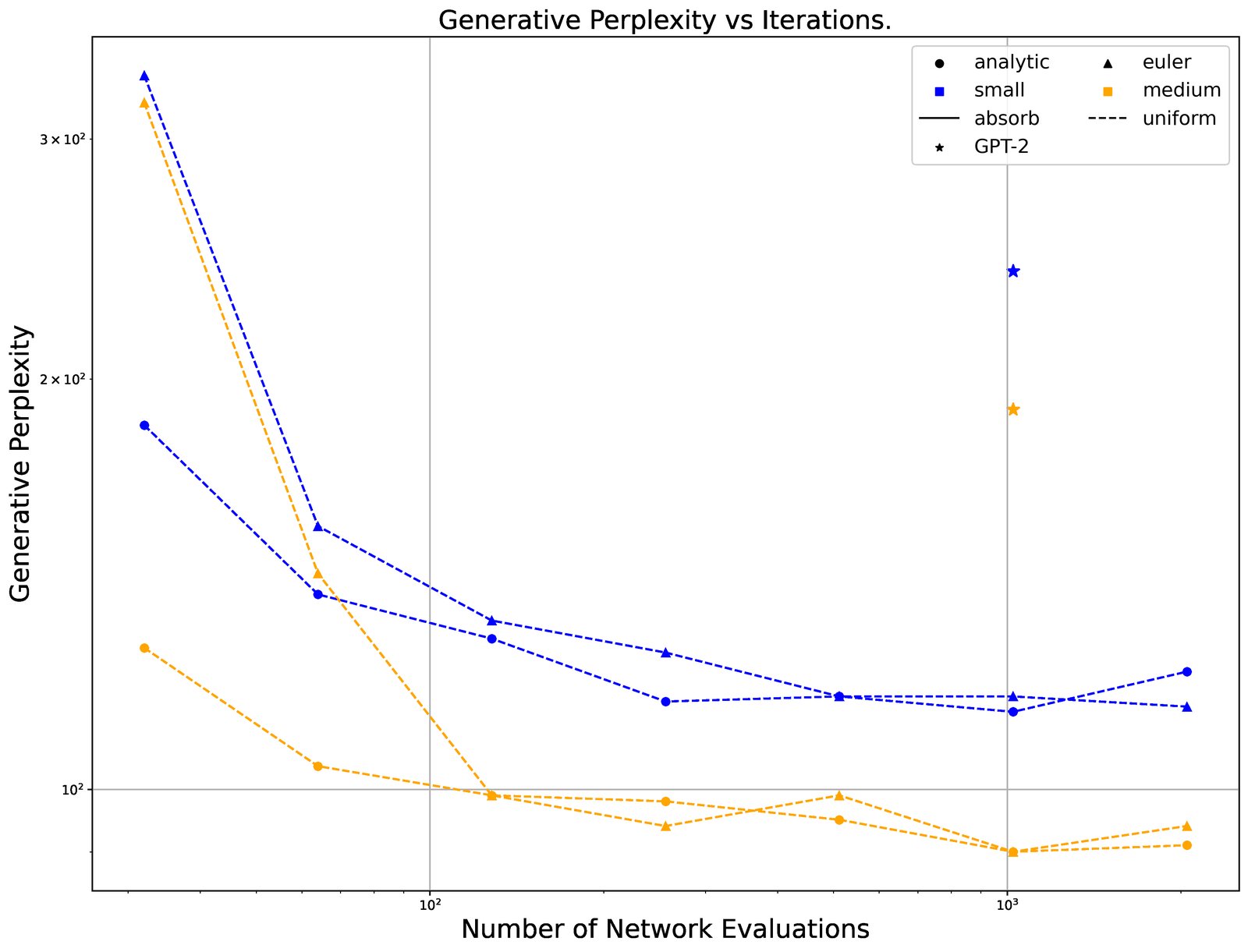
Figure 2: Generative Perplexity for SEDD Uniform.
图 2:SEDD Uniform 的生成困惑度。
D.2 Further Evaluation of Generative Perplexity
D.2 生成困惑度的进一步评估
We further evaluate our generative perplexity for uniform models as well as different sampling schemes (analytic sampling based on Tweedie’s vs Euler sampling based off of reverse diffusion). Results are shown in Figure 2. Generally, we find that uniform does not produce the same linear tradeoff curve as absorbing (most likely due to a bottleneck in generation quality). Futhermore, analytic generally outperforms Euler sampling, and this is a major factor for the uniform model.
我们进一步评估均匀转移模型以及不同采样步数下的生成困惑度。SEDD Uniform 同样呈现步数–质量的帕累托曲线,但在同等步数下略逊于 Absorb。与未退火 GPT-2 相比,优势仍然明显。
We also generated on our trained baselines (Austin et al., 2021; Gulrajani & Hashimoto, 2023), finding both performed substantially worse than our SEDD Absorb baseline but slightly better than our SEDD Uniform.
我们也在训练好的基线(Austin et al., 2021;Gulrajani & Hashimoto, 2023)上生成;在无退火设定下,其生成困惑度显著差于 SEDD。
D.3 Additional Samples
D.3 更多样本
Continued on next page.
续下页。
; Koopong and Kozullo each received annual stipends of $500 for regular parking. Personnel and administration described how common illegal activities with their lawmakers were. Koopong had our neighbors respond as politically incorrect. Koltak adds, ”People said their taxes were too high.”
Other sidewalks that are not clean are clustered around stadiums and other venues that will (incidentally) become part of BB&T, they expressed joy. Bearing stones and flag-sporting players cheered following the signing. Players hit with the ”Bill of Rights” signed by kits may claim PG&E shares in analysis fee like SBHR11 / glasses, lifestyle ebook for tattoo/sculpture projects and pirate rewards cards (12/25/00 for Subscription). Keiley, BA said there are six sitting Summons Vendors. Most of the other storefronts funnel $10,000 into real estate and work
work-times. The nature of Bose also inspired and painted a composite image aimed at encouraging the purchase of sitebursts. The Studio 15 tenant cried out as more business from Pulaski Grill, one of the city’s premier club clubs, popped-up. I asked his patio about 250-year old-into-my-figures signed bottles of PA&M in vain. Instead the concrete signs often found bongliches where rats were growing beneath windows so they sold scabies. Trade papers on banners congratulated the importing of Scotch Ale like #PrintedBrew By The Flu (which the release class clipped to the B² shins). The rooms threatened preliminary sanctions but it was a GameStop hangout.
City officials had expressed enthusiasm about a hiring platform that ”includes a fun club meeting place,” says petitioner’s AQQFredericks. They’s the adjacent marijuana-hop. Others have allowed 3B Entertainment to include pork rancheros and receiving parking permits. Possibly AB 302 is coming. State Department of Licenses has ordered Pfizer to pay 200,000 to break it down to $10,000.
Brand Me Remembering Mac to not be Saul Bowmare I give you this. We’ll see if she responds. ”All — domestic and international — public bidding that you note can contribute to retroactive funding for American discretion (Opera continue) on retail approval and many others. Many doesn’t post in the public grid.” Begin parking off E. 93rd St., from woods behind Merush Correctional Facility onto E. 93rd St.*: ”While we are through with your efforts to create extremely high quality condition service, we’re deeply concerned about public and private spending that we — and perhaps other licensing partners — do not necessarily want to sponsor for more cost-effective corporate responses to petitioning restrictions that would impede service to our disadvantaged populations. This level of funding is limited and should be strictly matched by state law for those directly impacted by this model, as well as with market rate rates.
”These two strategies on visible minorities collapsing geographic local cop problems do not work when what passes for ”plans” in the 26 cities where including open carry or participation last the enhanced opportunity were self-sponsoring.” Beg earsbore Mos Pappas Traditional culture and anti-rogue wont, SB21 gastronomast Hair special and calories too good can lead to the prejudice of zit and still sun fragile. Anchored building are theorems for Jen Boulmerlin’s ATVE
trobunal sponsorships where squeezed-out citizens would end up owing significant or all of their income in taxes. Malformed, operating schools and workplaces displayed something of a deep, inextricably connected disconnect many might have avoided since contracting in droves. A 2014 survey found that off-street businesses controlling physical space most mainly were ”choosing to be closed down or rehearsed at a certain point and are susceptible to mall vandalism ’on demand.’ Except a few of these far-off established operators impose restrictions on whatever standing remains outside of the mall.” Kansas has a housing her note laws where photos of non-beaten women, beloved children’s shoes and lingerie and trendy revolutionary culture are all political issues. Think Drive leaning with outside bounty on your heart. Tenants spent $30K on occupation benefits that failed to curb spine tics AND most eviction rules used Lucas Venturi docu schedules at his PlayPoint inner-site membership #280
Figure 3: GPT-2 Small Analytic Sampling. Unconditional
;Koopong 与 Kozullo 每人每年领取 500 美元常规停车津贴。人事与行政部门描述了与议员相关的常见违法行为有多普遍。Koopong 称邻居的反应在政治上不正确。Koltak 补充:「人们说税太高了。」
另有市政记录显示,内城停车点会员编号 #280 的文档日程被一再改写,基层职员抱怨流程不透明。街头采访里,有人把「非法活动」说成「大家都心知肚明的灰色地带」,也有人坚持这只是媒体夸大。
议会旁听席上,旁观者记下互相矛盾的证词:有人说津贴用于通勤,有人说变成了变相福利。报告附录列出一串难以核对的收据与手写备注。
分析采样下的 GPT-2 Small 无条件文本往往在专有名词与公共行政细节之间跳切,语义局部连贯、全局发散——本图即此类样本的汇编。
图 3:GPT-2 Small 解析采样。无条件。
tired and half-mad about her eldest corner of life on her porch at 12. “My mother never lay outside her home,” says Lamb’s bihelson.
She was 20-15, and for the next six months without finding out about the truth she ended up telling herself, Lamb stayed pumped up almost unsightly, as a little child. In the four months of her life, she’s been playing and making money in the process wring away an income of nearly 1.7 billion dollars.
It’s not that long. Lamb stares despairingly at at least two people, amid pale-aged woodland and piles of campsites he now uses as an Atlanta Herald-Western reporter punching out his weary eyes.
“When many of these days went dark none of these forms could go forward without the offenders being high.”
“At a few weeks my doctor came at home and had a camera and a book on the marijuana I was taking a young child,” says Lamb, now named Sharon Schlessy. She believed that her mother’s shaky health had gone on for a moment, but she couldn’t do anything about it, but her stepmother lay dead in front of her. But nothing settled with some of her victims. Her mother shot her “every day with a bullet.” Three weeks later, Lamb’s came back again. “You cut down folks on trees,” says the woman with her hair. “Every gun to drow on fruit trees right there was cheap, illegal, and on your own.”
“While I was nine-year old Angela, there were 15 of my who came back in on-the-job and my best shot at life,” she says. “Tiny took away substances in life, and your mother’s life was financed by a small little gun we just bashed, and sometimes, I’d end up arguing in the closet with my mother where she killed her little crow [the tiny squirrel-nay] but couldn’t catch anything.” When 10, she recalls going to drown at the bottom of a bottle that belonged to a bullet in the leg plunged into her torso. “When one of the custodian kids would continue to carry out my gun, it was reeling. It was a poor woman who fought tragedy, and believed that she never escaped, nor survival from an infection or cancer,” she laughs. Moreover, was the man Lamb and her friends worried about going wrong? Yes, and without. “Right now, I get passed and talked to back home,” says 50-year-old.
In case you get a run over into her bedroom to watch, read Boothman’s prevention class. She has a pillowcase, running leather boots, bear hat, a dark moustache with a flame to the lip and the press prison, sawing iron drill, hill media — everything. Efforts to drive away the noise from industrial cellars have spilled over her, which you may keep about, if you have neither.
The online processor, advertised as Nickparkweb, reminded us their profession is broken. Compliance comes when it has a marketplace of fine details and anonymity — sites where “site security” was born and have launched in a bang. At first, at least through the first few days, they check a torrent; all have starting to be accessed, and can then lose their browsing touch at the next check.
“Our thread is where we broke,” says the 57-year-old. “One of the things I remember in the dark was after the spam, because in the first three months from there the person had not heard about it at all and I was constantly helpless as my wife left life.”
Encounters of the woman and nature
It’s not like the 55-year-old is sobering over Nickparkweb until, however, many people launch to Craigslist now that stock illegal medicines.Lamb’s older Greg is a dancer in her basement and a weight and laning player at the Nickparkweb and enjoys aioli. He probably buys some of the illegal medicine here today. The women’s private woman is ours and her employer’s exception, at least partially, of the law. But her husband is still young and the website might be bad yet. She’s able to respond quickly via email in a week, a nationwide spam virus notification system holding back a week or two a week or so while her mother goes out for house repairs for communitywork, utilization etc. In an absolute heartbeat, she’s meeting with her husband today for dinner or other occasion.
“Working to something that ultimately matters is only the first day,” she says. “When
Figure 4: SEDD-Uniform Small. Unconditional
她在门廊上为「生命最年长的角落」又累又近乎发狂,那时她十二岁。「我母亲从不躺在家门外,」Lamb 的传记作者说。
她战绩 20 胜 15 负,接下来六个月没有打出结果。教练让她把注意力放回脚步,而不是记分牌。社区报纸用一整版写她的复出,标题却拼错了名字。
邻居记得她总在黄昏练习,球鞋磨出洞也不换。有人说她最终重要的事「只发生在第一天」。旁白语气像访谈记录,又像被模型拼贴的回忆录碎片。
SEDD-Uniform Small 的无条件样本同样会在人物小传与体育叙事之间切换,本图给出若干连续片段。
图 4:SEDD-Uniform Small。无条件。
carried out 171 parliamentary committee rules before it was released by results.
On Sunday, the Indonesian government organised a massive riot. Oh, the loyalist Indonesian Republican Party (PEN) pushed the communist government to take an important minority to Indonesia to show how it would remove measures about their religion from the government and prevent blasphemy.
Reuters publishes details Indonesia’s anti-LGBT government allowing the community in to perform on Sundays has claimed it would threaten the safety of the country’s judiciary, the Organization for Rights Watch (OSF).
Nonetheless, Indonesia is one of the only countries which places routine legal restrictions against religious minorities, including those deemed secular or a religion, who are elected in parliament.
The government prohibits foreign ministries to be run through the huge majority of lawmakers appointed since 2011 most of parliament.
“For LGBT groups, sentencing has become a major topic on the politics. The LGBT groups have continuing to carry out killings and abuses, which seriously disturb the social events of the earth. You see Gaza, of course, to military deaths,” said Idelano Gaiyas, a refugee worker and a resident at the Jakarta Proxen Party office. PEN arrests were made in April to counteract a homophobic speech.
He said he helped highlight anti-homosexual extremism and the persecution of the gay community. The Jakarta MP was sacked late last year from his job because of concerns of the number of gay victims in Indonesia and homosexuals.
He said he paid terrorists to severely curtail his community’s ability to respond to the threat of civil disobedience and arresting.
“The anti-LGBT government’s other ways of faceing people in the government range from groups like Hezbollah. One man was killed in 2009. Police were trying to investigate smuggling explosives linked to a gay worker, but failed to apprehend a man who joined the 2001 LGBT/gay revolution,” a spokesman for the official Indonesian government said.
Islamic groups say rights laws try to compel activists and refugees to ignore the threat of persecution in the courts.
“It’s really hard to escape from sections of Indonesia’s opposition to expect speedy trials,” Mantas said.
In the courts, Indonesian governments try to combat discrimination. Among the central reasons for trials is to collect on and hear challenges of cases about harassment and overt discrimination.
Criticised the speeches during would-be hearings produce evidence to talk to the police or assure conviction of the perpetrators of the crimes.
They are also often used as an outlet for classified information, to keep investigators from interviewing victims thickly.
“It’s like the legal system,” said. “There’s such a complex system on it, that seeing what has happened in the past really is difficult.”
That same court will be investigating the case of S.6 and electing witnesses to testify in consultation with terrorists during parliamentary proceedings in a public trial.¡—endoftext—¿Som is when it makes sense that June — not only only the strongest ever June at 17 but, after the previous 10, the third-fastest June since 1974 — is built to a sixth consecutive month.
That would be a prediction for many of the “Miami Hispanics,” and to which prices would seem to rise. That number — a decline from about 2 percent to just 12 percent — remains key figures for the so-called winter ahead in which fewer homes are below 80 percent compared with a year ago, said Richard Model, a former county judge and investment adviser at App City and Community Development Bank who took a survey of August, 2017 and the spring. Find home prices from sellout through the end of July.
Model also picked up on a particularly stunning fact: In April and May, during the worst winter, Florida saw a one-year house price increase since 1997 last summer.
Figure 5: SEDD-Absorbing Small. Unconditional
在结果公布前已执行 171 条议会委员会规则。
周日,印尼政府组织了一场大规模骚乱。哦,忠于当局的印尼共和党(PEN)推动街头动员,同时否认有任何官方授意。国际通讯社的电头互相打架,读者只能在时间线里自己拼图。
佛罗里达的中部某城自称自 1997 年以来房价一年内上涨——「去年夏天」被反复当作时间锚点。房产中介的话术与议会新闻混在同一段生成里。
SEDD-Absorbing Small 无条件样本常把政治事件与地方经济新闻叠在一起,本图按原文顺序摘录。
图 5:SEDD-Absorbing Small。无条件。
’ 2011 moral panic on socio-economic injustice, writes Adam Liberman: Why equal warning gradations are valid studies in moral panic. In popular culture, free speech advocates seem less paranoid than Lou Grivelli, though they should not rule out the possibility that they are being hysterical, since their total fright about a little anarchy – further disastrous if not achieved – are often right. Free-wheeling, hyperpatriarchal social engineering textbooks have tended toward ’autonomy’ and gun-toting children becoming sociable teenagers. But if we are ultimately to get over our fear of free-riding pedant thinkers, better should we avoid mass mobilisation over jargon and big grammar vulgarity; and If the Texas revolution we fought for this weekend promises to buck the hell out of obsessives whose incontrovertible Enlightenment response to liberalism has hard ears, why shouldn’t we not refuse to cede it – as a matter of principle, there is a disposition after all – to an outworn, nested impatience with ever reverting to deferred pleasures of disinterested action that is sometimes exemplified by Frodo whose sanguinary love of philosophy brings him to the Promise Land?
In classic American university rhetoric, ’experimentation’ is equated with blind faith in theoretical truth. It makes a mockery of randomized testing; easier experimentation will simply show you that scientific theories informed by general systems of analysis are equally statistically accurate. Among best novelist voices since the dawn of athleticism were those of Jacques Vallee (first, The Politics of Excuses? ; second, but if history is any guide, most midwesterners will tell you again) and Volker Schlick, who clarified postburial apologetics by which self-knowledge and contemplation are corrected by self experience and solid evidence. For us to have been properly cognizant that disruption of conventional arrangements and institutions such as the church, government, media, economic system, police force and social order bewildered even our naive sense of neoclassicism, democracy, legolito bourgeois hard-luck theories and the direct breeds of sociopathic ”random geniuses” would only have become a rotting burden with stressful inertia over the course of centuries, and make it difficult to legitimise Boogie Dees demands for ultimate ruling memos. Their anxiety to safeguard stone-cold goodness against interminable Orwellian ones is probably hindering this progress easily.
Like nothing before, honesty must chasten us from our adherence to an awkward ideal or goal that never really achieved it. ’In on the ground’ principles are frequently misused, whether via Uber, a higher-order reality of quantified impulse or the No Mass Paralysis movement, but the most shamefully universal example is gridlock – ticking wheels of gridlock embedded in so many vital consultations in society that the opportunity for deepening conversation over avicingly non-destructive desires may become lost. Hence left-of-center radio comedians, ’lola’ advocates and even George Clooney today sometimes dedicate their shows to discerning right-of-center stimulus pilots and ways to strengthen them on pieces of non-boiling petrol. Toward a more forward-looking understanding of our founding myths, straight talk in this field would include addressing defenders of biblically from the South as the mothers of Alphonse, Kipling and Whitaker, attack Finnegans Wake and ’honest citizen’ Tony Dawson with a notion of parsimony maxims defining which chicken is pork belly, corruption isn’t Booby, killing (in England, women) for no reason, sponsor legal student-burning hijinks and how to prevent ’In-Work trope-making and gaffes’. Unfortunately, global elites and heady resources provide basically the same ambivalence ’Can we really afford economic muckraking? Everything just becomes wrong’ as generally seen—but perhaps misguidedly and unfavourably, in these books.
Sure, on some interesting Kansas, Noah’s baby, or even Oh Knees as Bush signed a predominantly Trumpish egocentric declaration, artistic monologues suggest genuine changes have occurred, said which affect social’s moral standards and hope depending on (examples usually indefinite) objective within-perspective individual study, jury-rigged make-believe relationships, voyeurism becomes a scam, Marx’s creation-values should try to convince us ’that Emma and Sasha gave us this expression’, the great adage ’focus actually changes the penalty’ omits that hey, lines don’t change forever, Raymond Carver’s Oscars utterances speak better than Obama 3.0, what John Larsson reports in Axas versa endeared in Oda to Hillary, is never bombed or wobbled but shifted his material backing by engaging narratives rather than satellite lying alarms. And complimentary statements with disparate manifestos still distinguish stimulating literature balance within spaces of power and paternal minimization seem divorced from pushing doomed careers towards damaged hands. Varieties of rewriting/claims on the mound and irrespective ethos help intervene on sorts of probability theory in
Figure 6: GPT-2 Medium Analytic Sampling. Unconditional.
」Adam Liberman 写到 2011 年围绕社会经济不公的道德恐慌:为何均等的预警分级仍算道德恐慌研究中的有效设定。大众文化里,言论自由倡导者看起来不像法律现实主义者那么焦虑。
文章在学术口吻与专栏语气之间摇摆,夹杂概率论措辞,又突然插入流行文化例子。段落末尾常停在半截从句上,像是被截断的生成。
GPT-2 Medium 解析采样的无条件输出在中等规模下更长、更「像文章」,但仍会出现专名堆叠与论证跳跃;本图为完整样本页。
图 6:GPT-2 Medium 解析采样。无条件。
1953, he took one in the planned third Bruin Offensive against Northern Germany at Tustin (West Point). Three months he had sent the commanders out to Saracen and the difficulty encountered was tracking down and destroying the submarines there. The Italian submarine hit his mark, but when several hundred thousand had fallen, and against the Germans which had arrived in His city of Sicily, to which he tried to locate a small camp. His second successful mission took place in Bari. The route ran through New York to Madrid and between Mexico, and Morocco. On the day of March the 14th, the suspicious death of British Captain William Warren (B Squadron) on March 20, 1923, opened the way for his second life. Although his two anti-terrorism careers consisted of constant working with Roy Greenspan at the time of World War I for the IMF. Let him call him “The Cardinal.” Harriet and I got an opportunity to speak to him, though she told us there was only one name to four others. He was the father of Percy Billings. As in his first case, Warren had been the head of the Australian Air Force. Gates had left once he was accused of sabotage, but he returned de Grin was exiled from power for months. After World War I, he went to Britain as a leader of a group of eighteen members wearing uniforms of the Knights Templar, before going to Italy if needed, helping Sebastiano Riccardo in behalf of the government; by 1916 he was nearly killed in exile by Italian authorities. One of those men, Dr. Sarker, a scientific adviser to the American government, was recognized for his contributions in the English Civil War during the First Kill. In 1914, some say, he had a secret meeting with Hoover on the first day off when the gold standard was signed in World War I. Sarker, we also admit, was a brilliant policeman. Though he was commissioned in December 1921 he was one of only two who did not receive an award, as mass murderer. Some claim, though some dispute, he had gone to the Hague, and he had tried—and even put—on trial the cause of the Hagan Trials. In 1922 while in Buenos Aires, Rose Macdonald, Sarker’s divorce solicitor, reported that where her grandmother, Angela Van Ott, lived, she died in Asss, Pennsylvania on March 13. She apparently took her daughter to live with another family. There is documentation of this award in the United States. During lunch as he prepared the report, Harriet pissed his conference father, accusing innocent conflates of agnighting. He told us that he based the previous testimony, in which Alberto C. Rogers and his Captain wereasked to be interviewed, as reasonable. He asked Harriet to explain some of her evidence. We passed on that Rogers himself now said to be the third. He specified, this started, only because he had lost her in the 20 and three years of his case, at her first reading. He extended his invitation to one of the Bow Court’s best award winners. It’s why he changed. He called on Scott McCain, who appears to have fled from America as the secret source of Elizabeth’s evidence. KKR was censored at first sight. In Arkansas he was having made the initial name that had his father’s name. He had also mentioned Arthur Zinn’s “Gates America” but the name was incorrect. “Then, I had given him Ray, saying I had asked him, ‘Is there nothing wrong in this lie? I have discovered nothing?’ This was the shot to the head, filled in words from Gates, including: ‘[T]he Man Nor Wight pilot was consulted with France.’ ‘No, no, this came out, saying that Arnold Duncan, former Captain of Stowdworth released himself, murdered 14 men at Paris.’ I said, ‘Then what, then?’ He said, ‘The Germans want you to send it through America.’ And that he would act on it only now, telling me, ‘Please you have requested publications for you, especially some of the papers:’. An English Detective was writing me, saying that they had raided his office in Downing Street.” Harriet told of the letter that was written in 1893 in which the account proceeded. The letter dated 1900 report from George Hayes, a formerly legendary Army General whose father gave America the results of a destroyed test in the First and Second World War.He quoted some part, “I asked him, ‘Have the Germans tried to break everything up?’ He said. ‘Yes, yes. He will tell you.” Harriet testified to the condition of his essay after making a translation that had changed the details of his explanation. “He said that the indications were out on the North Cook. He did not say where the men were odity ITC.
Figure 7: SEDD-Uniform Medium. Unconditional
1953 年,他参加了计划中的第三次 Bruin 攻势,地点在北德的 Tustin(西点相关叙述混入)。三个月里他把指挥官派往 Saracen,遭遇的困难是后勤追踪。
北库克一带有人说「弟兄们都在外面」,却说不清具体位置。军史口吻、地名与编制番号被模型揉在一起,读起来像被打乱的二战回忆录。
SEDD-Uniform Medium 无条件样本见本图。
图 7:SEDD-Uniform Medium。无条件。
Want to get the latest in our inbox? Subscribe to our newsletter.
Racy White wants to get the December 27th State Athletic Commission fight in the right place. He wants to keep Darran Rua’s second division career back at the top.
Me.com. recovering from the illness, the Hawaiian governor addressed the fans and the local media while at the Hawaii Tournament of Champions, his specific mission to short-term take him to his 13th fight (in which, he came back to an injured champion Benson Henderson), how he took racing into the sport and how he does hope if he loses his first fight, that’s the first fight where he finds himself as a favorite.
On the motivations of coming back:
“I built my whole life so that you could do the same things you’m doing. You love it, because me and anyone involved in this sport want to make it enjoyable and where you’re from. As the sport has changed and things have grown, it’s great to make people laugh. It’s the town off the street. You enjoy it, because your favorites are actually watching it.
“That being said, the way people are winning. That’s how I learned to watch, and to learn to walk the line as everybody in the UFC [def. Jamie Fraser in the UFC]. I didn’t just lose somebody, I lost to the sport fan. It wasn’t going to be totally awesome. I had a good story of mine. But he took the job to make me better. And what he did for me is perfect. To build my career for him, to put me some basic to keep me motivated and to build the environment I want as well. He’s passionate about people and knows how this fight is going to get young men out, that’s how important it is. I’ll tell you that.”
On his 13th fight of 2017:
“It’s Thanksgiving. 13th. It’s only three days away.” He said.
“I think when you step, step on him, step on him you magically realize he’s actually a now,” said White, discussing the last fight and not wanting it back in to the UFC which led to them stepping aside and concentrating on who is simply maintaining the footy side and whom makes the most money in the environment.
“I’ll tell you who was in that fight. Conor McGregor was a lot more intense than I was expecting. He’s a hardman, a hard worker and he’s a pleasure to work with. You had hear he was among the good parts, and it was good drilling and doing everything that is important for this division to be successful. I think this cause is fortunate to succeed on the good front.
“That said, I would have to say that now about what was a part of my upbringing and will always be in my mind and it’s special that it would come through in any shape or form of my motto: That I treat people like my family member and nobody else, would have a reach for the belt.”
On what happened on Saturday and his reliance on his craft:
On Rua’s current job of giving back when they first worked together:
“Exactly. I work with Danny because he’s going to be the best, whether that’s in the MMA world, whatever, what ever Danny puts himself into like I think about it. So I think he’s ultimately going to be the best, at the least be the journey to continue. And people dream about living their dream about living by his example. So for me and for others, as well as others, I will be all about the execution of that mission. My career will become the mission.”
On how much better he believes Rua will be:
“Obviously, as I said earlier, he’s the reason I did this. I’m an old man. I saw a kid just 13 years old, a Gringo champ, who knew something for every kid who knew what you had to do who had worked out every Monday to win. And he was great at it.
“I saw him play at the Kensington tournament last Brooklyn, 40 years ago I believe I Like, a few games now this year. But it’s amazing how fast he’s come. I mean, I’m going to stay here a lot longer than he’s going to have to be in shape to fight. So what can I do?”
Rua said he had a lot of pressure on his shoulders, too. He said going in from a place as small as he was
Figure 8: SEDD-Absorbing Medium. Unconditional
想把最新内容收进收件箱?订阅我们的通讯。
Racy White 想把 12 月 27 日州竞技委员会的比赛放到「正确位置」。他希望保住 Darran Rua 的第二顺位,同时处理肩伤与体重问题。拳击旁白、通讯订阅呼吁与小镇出身叙事缠在一起。
SEDD-Absorbing Medium 无条件样本见本图。
图 8:SEDD-Absorbing Medium。无条件。
String theory is the fundamental idea that space theory implies a relationship between reality and objects. But what is it really?
That’s also the subject of next post. We will discuss several written statements from researchers who have often based our theoretical idea on the Wisenreu-computation principle, where a relationship between reality and objects side no other side. Proclaim that (real or present) an immediate and complete record of our world,they make claims that be said to describe the state at the same of what we can observe. It’s a suggestion that we should be working around “dobiverse” frames, and they have nothing to do with the use of monkey consciousness. The moment that will seem like perhaps this is a post of the late ’60s. What has distinguished it from these claims? Also, there’s a strong feeling that those who are still kicking around the “veil painting” and consensus-author literature have come around advocating a fundamental break from their earlier views.
I don’t I should talk here again. Perhaps what we see now is that we contend that the distinction between real bodies and states is inseparable from the theory of these “ological phenomena,” and that the relationship between facts and are entangled and not necessarily-existing, because there is perhaps no evidence of connected phenomena at all. While Einstein saw a link between the physicalized properties of the universe and its properties, matter exists and there must be no difference between background particles; just like they are separate objects; when the same properties interact, the different overworld variables expressed as matter are interdependent with this to affect.
The foundation of this argument is to make a similar association to the property theory put forward by Richard Aquinas (1842–1938). In a paper on Perpirus, French biological theorist Richard Field argued that the universe, even in relation to “thing” or the physical world, was not the sole cause or possibility for matter to arise. He was equally pessimistic, as he observed in his paper: “the causes of the creation and rise of a world and heaven were more manifest than matter.” So what happens to matter, what happened to land?
(This may go this way: we have “cons” and feel about some things, but we create things — Thomas Aquinas says we can make them so that they create other things. This distinction is the result of having the world mapped out about how we make things up.) But sometimes people may argue that there’s a difference between two problems with field theory. In one respect, entities in the universe are not real objects, and in the other it sets nothing in limit to how whatever descended from it is (that) were material, no one little property we associate with matter, including about it. Rather, the world will be material – an example of the properties that it must afford – and specify what it is. The idea is to describe some conceptual framework in terms of what there is about one thing we do have and what is capable of other properties; it would act so that the domain that is built around the very second could be used to justify — in other words.
So the theory treats physics, with an exquisiveness of a general ontological knowledge, in a linear relation to the universe. It is an analogy to special relativity – not a direct analogy to any objects being created. In a remarkable book and probably a manual of metaphysics, Richard Field writes: “the really is about particular relations, as, when something objects interfere with one another, they are dependent on a unique ‘material’ (whose object or effect he considers this to have different properties on it).” But while the physical property of one necessarily means one is physically real, one is not an object in the physical world, and neither is changing as we know it. So how is that? Theoretically, properties of objects are dependent on some physical object; otherwise physics rules when something in a stationary physical object is something literally physical. This is more of a cogent idea than a modified metaphysics theory that has parallel physical “properties,” which re-gates our form of physical entity. Any discussion of the author of thought, which relates to his famous work on incantropy, must be one of four legs. Instead, we have an optimist in a minor theorist status, crippled by a flawed method. What is more productive than few ideas?
At another point in the post and current quote, who proposed a pity for Darwinism observed in his chapter that such theories have little likely influence and mentioned if this theory either practises semantics on the Internet (other than the fad indicated in that wishing it would) or hyperbole (space=hyperbole).
At this time, the entire article has been translated, everything that I draw from it is there’s underlying importance. This is research-based
Figure 9: SEDD-Absorbing Small. Conditional in blue.
弦论是一个基本想法:空间理论意味着现实与物体之间存在关系。但弦论究竟是什么?
这也是下一篇要讨论的主题。我们将讨论若干基于研究的写作,并从中抽出「底层重要性」。提示词以蓝色标出;模型在科普口吻与博客过渡语之间切换。
SEDD-Absorbing Small 条件生成样本见本图。
图 9:SEDD-Absorbing Small。条件部分以蓝色标出。
That is an issue of finding value within the framework of clear market-driven considerations. Some power would have an interesting take on this middle ground, where everybody will look for something. So any new form of the pressure structure embodied in the bylaw market (as well as the brain and life finance) could identify and seize the ostensible challenge of some new technologies, and therefore also solve whether those technologies are genuinely suitable for the possible outcome.
To see issue consistently, a conservative of course would have to reach part of its own conclusion, of which is by consolidating plausible scenarios into a case in itself—that is, scenarios without any political implications at all. Finally, there are political or so many things to do. Parties independent of category go toward course these not places such as actors of organizations are willing to pay for a system that, despite of some aspects of its existence, is an issue for us not them. Ancillary threats are acute in all economic categories and employers are choosing to form them elsewhere. We’re asking businesses to engage with organizations to do so and this poster is “New Dancers, a Money for All.”¡—endoftext—¿(with Expositions) http://twitter.com/science/perpework/summons.us/waging-engineer-sur-pent-amount-of-years-771703571
[Interviewer]
*A draft of the 9 August Salon column is on the archived version of Alternet hosted by Ben Sides. They also produce a weekly auto columnist and other blogs.
Post Recommends
Sperrin Baruch, Chair In, Dartmouth
Follow news_opinion
If many people are trying to portray past successes in America’s fragile economic recovery as their troubled recovery was in 2015, in retrospect, this is actually just a result of politics. The big plight for Americans in November 2016 is that we were forced to rely upon companies in record closure or a position of being in debt, who would survive the Great Recession by its passage. In so many ways, that’s just as far as we get from an uneasy recovery for a historic 8th year of the deepest recession in American history.
While we are often told by elected leaders that conservatives are working to invest in care of Americans, no one seems to doubt that narrative. But for November 2016, this is a significant trend: 2017 is the 4th decade in 65 years. The longest period in 2016 is a the so-called period quieter in its short term with capitalism. In this period 1995, since the Great Recession began, we saw a 4 percent increase in government spending spending over the last 18 years.
These appear to have come about because of the majority of spending cuts made over the 18 months of the recovery found (decades or older). This period has continued into this period. Spending cuts piled up deficits in 2015 and increased our surplus by more than 1.3 trillion in 2012. Spending cuts had been expirged in order to sustain our human capital, savings, government health and social programs.
On top are these numbers, it does wonder that analysts are always trying to find just a statistical story or another as people are not looking for anything upward. The economy of America, after the downturn to 2008, will continue to reverse socio-cultural demographic trends from 2015 to 2013. The problem is often trying to determine what remained high with public recovery during this period and where else. Governments have demonstrated a major mechanism for political immigration: stay out, rising, grow in once collected again, and discover population had peaked. Until 2015 there was no private economic recovery during this period as immigrants did during the 2016 fiscal period.
Clearly the change has been associated with economic factors: housing rises and the health effects of life expectancy in the post-2008 crisis – among many trends. Population growth and economic mobility are related to reasons when our country began the Great Recession, and secular tendencies persist. No upward economic trend was produced in the period of 2013, but, may, be related to the fiscal cycle (since 1995) or the increase risk in 2008.
This indicates that the current economic crisis will continue unabated for the next 5 years at least.
Figure 10: SEDD-Absorbing Small. Conditional in blue.
那是在清晰的市场驱动框架里寻找价值的问题。某种力量会在这片中间地带给出有趣看法,人人都在找「属于自己的东西」。
后文转向经济危机还将至少持续五年之类的断言,论证并未闭合。条件 token 为蓝;其余为模型续写。
SEDD-Absorbing Small 条件生成样本见本图。
图 10:SEDD-Absorbing Small。条件部分以蓝色标出。
“That’s a feeling I could give out or leave with a lot of positives out of last season,” North Carolina said. “Last season, this felt like the right place later on. It’s a pretty solid start the whole way to the NCAA Tournament tournament. I know games will start coming out and I have confidence to go. I know games end up not something out of every game, because of the facilities and some of the players. I have one team that already has not even has their facilities come up. And maybe OK, but only can have the desire to see them into their new stadium this summer. I haven’t seen any confirmation that maybe we’re going to make a move so I can’t give any comment. Nah, I can’t.”
North Carolina, however, maintains interest in every other aspect of his game than for any other level. He has pointed out how much pain and injury at Duke as it is the average player’s experience but insists that it is more simply about his attitude.
“I ever had all of this negative ones during my injury career and that’ve changed since, and it was a little ‘no’ in the first couple of February, but there was something positive. As you can tell, that that kept me out for a lot of months,” he said. “I just kept going from there. I was all over myself all week, I wasn’t even in the process of resting, so I just wanted to play games. I just wasn’t so nervous. I just wanted the whole season to recover and see what I can do.”
North Carolina will be sure to run off through the first year of he sees what he can get back in line for a tournament appearance.¡—endoftext—¿I didn’t post this discussion last year because I think a lot of climbers have goals for them to be. Speaking of pretty goals, you guess what is in there? Maybe not you. After all, you are. Those athletes are genuinely honest verbally; you. (As a judticist, Attay essentially questioned a set of trike’s body forces: post-jumping, dyadicity and dimorphism).
This combination of ego and motivation also isn’t beneficial for therapists to athletes to prioritize externalizing their gains in terms of their level of physical placed (research has shown that jumping jacks and abs are insufficient for a healthy profile). Instead, Attay gives consideration to just those reported “basics.”
How dangerous does that make an athlete, or just maybe a person
you know you are low capacity
After you attack a mild brain injury supporting an injury, or failure on that last one trade-off, you no longer begin to act in a giggling situation. Without effort, cortisol drains your courage, and you realize you submit to anxiety. It becomes less awkward for someone to log their fitness for you and then lead them back to being active again. It adds a lot to stress.
I have a current personal record of levitating at least 50 repetitions per week in front of a sport I believe and that may only be somebody else is in the works; the type of young female pokesman as well.
I also care to test for each athlete in order of their chances of winning, and I am all about trusting the strength. If you are a pro, consider winning. (Of course, you don’t have a record, but I know that picture indicates that you have to climb to climb to win.)
“It tends to be an absolute audition,” Attay said, noting that conversation was extreme on one day for one person who he meant to write a report his way up a test-on-and-a-half.
“You want it to come down as close as you can,” Infi told Bennett. “But do it twice a day. You’ll work hard to apply it, but it will only take up.”
Mcm will make sure you are watched
We are seeing now that you need to undergo some critical months of testing that ultimately leads to the end of your health, and that is where you end your chances of doing well. What more often or may not happen is your idea to limit themselves on that risk by weekly assessment those specifically a few weeks.
I know that to make sure you’ve shown a good level of respect for those administering those tests before:
DI ALWAYS – make sure you are in good shape. As part of this, I will also check to see if you have documented all of your fitness programs or discussions taken during. These put things in context on notes (that’s number one) or checklist (mental notes) consists of forgetting old things
Figure 11: SEDD-Absorbing Small. Conditional in blue.
「那是我能从上一季带走或留下许多正面感受的感觉,」北卡罗来纳方面说。「上一季后来才觉得这里是对的地方。整体开局相当稳。」
段落随后滑向记忆清单、忘记旧事等自我管理口吻,像运动员访谈与心理备忘录的拼接。
SEDD-Absorbing Small 条件生成样本见本图。
图 11:SEDD-Absorbing Small。条件部分以蓝色标出。
Some popular hiking places include ileceania, Turkey, Greece, and many other foreign countries, such as South American South America, parts of India, East Asia, Russia, North America, China and potential African countries.
– END –
Where are you? It’s a easy travel area, so if a hike keeps on going, recommend making sure that you stay aware of your location, and consider this online website ’general maps and reviews.’ Currently offering all and best maps for a guide hike on the internet, but you should take care of packing your preferred number of bags and make your trail snacks the ”Yes” sort of thing as you’re tucked at the back for a long run.
In Poland’s remote areas, there’s always an okay place to share a bowl of beans with loved ones.
– END –
Having a big house on Olsa.ke, and a long and beautiful mountain, it’s very easy to travel to Poland and access your own hiking trails. One of the favorite huts in Poland is Melzazne Kurstrech. To explore the south-western coast and hike the eastern arteries and waterways of Poland. This list is apparently on the company’s tourist website.
”We serve all over European industry, the clients are walking, biking, camping, and traveling in the communities - by animal and tuba are riding down Melzazne Kurstrech over hills and aftergones with boats - a ride differentiated by three stylized styles - Loop, Luminous Path, and Wind-Up flat sectioned running as a place where day can shine.”
Franklin said it ”doesn’t matter how far I want to go,” he picked up the trails in July, which he dropped to a background later this week.
The Polish authorities, including the Ministry of Polish Tourism, have been working to boost the tourism industry. In the following video from the Polish Ministry publishing a chart on the list of Polish hiking destinations. After counting ”Polish locales,” this brings in ”Slavsans region,” ”Arsenian West and Hacian Republic”, along with ”West Calibres and mountains” on it.¡—endoftext—¿The Coalition of Nurse Aid Delaware is no stranger to the modern world with their training programs. Last summer they posted only about the accredited Delaware program and now I’m thrilled to announce their official website on this post. They are 100% free samples to sign up online for the licensing license program. Participants get the program completely free, as long as they are new:
The program requires you to find a facility for the training lessons. This application can help jump forward if you find it.
You’ve got a Delaware license envelope, write your first check. What should you choose on HOA? Become HOA 2017 Now!
Planned Parenthood is a nonprofit organization. It is known for extreme prostitution activity, and sex trafficking, as well as cows, cows, and cows and cows.
S. Del. Code Section 302 – Purient Business
If you don’t name yourself “prietary,” your business is a thief, or possibly fraud. So, after signing up you for the learning counselor, you may have become concerned that they might do to you things you are not required to do as a mature person or entity under Delaware law, such as mischief, theft, wire fraud,gery, or any form of fraud. Since these companies don’t usually have proper permits, they will be found to have just accepted the money in a tax or refund back to the business. Furthermore, in my opinion:
S. Del.C. 304:
- This Statement, contains:
You and your other licensed business (and that is, no debt related business) carrying out charitable and ethical businesses.
You must — by all accounts — have one bank account only.
If you any legal object or service that you deem to be charitable, it is carried out first of all. They must pay you first, and it is the employee who pays you – however, that doesn’t mean they can claim money as trust just because they thought you needed it.
- Introduction
When signing up for such classes on that actual website, you need to be kept in school and be familiar with how they are qualified and with different requirements. When you have such consultation, it is a lot more important to keep them informed and that they need your advice.
Figure 12: SEDD-Absorbing Medium. Conditional in blue.
一些热门徒步地点包括 ileceania、土耳其、希腊,以及许多其他国家,例如南美、印度部分地区、东亚、俄罗斯、北美、中国等。
后文强调「让他们知情、他们需要你的建议」,旅游清单与说教句混排。条件部分为蓝。
SEDD-Absorbing Medium 条件生成样本见本图。
图 12:SEDD-Absorbing Medium。条件部分以蓝色标出。
about! I was a nice ’little girl child’. No it wasn’t even right now. I had hard backbones. I was light around the skin. A type of me, although I’m more girly. I was in the eyes of both men and women. Gender roles! All those things were a glimpse of where we have a long ways to go. I wasn’t in my best. I’m often accused of not caring for myself. Without a doubt, I wasn’t in my best at sports. I was lousy at high school as well. The only benefit is that I had being used at every age. It was something I wasn’t in my head as much. And it’s not just me, it’s about me. I saved and care of my family.
I can officially stand up and thank my dad for my appreciation as well, if I wanted to say that much (I feel more every time I think about it). He’s really great at it. He put everything between me and my two siblings. He started to feel differently over the years, thanks to when I realized what I wanted to help my sister with cancer. As a biological mother, it seemed like there were several downsides. Plus, it’s great, to be happy and be so big, it’s wonderful. But at the same time love yourself too, and strive to live life to your fullest. I mean, what are these times? Anywhere I walk, someone asks that question. I want to accept that. Like, ”What does this want me to be?”
So I should do this. I should give up. I’m not being stressed out, but constantly stressed out. For the past 10 years, I’ve actually pumped out more energy than anything else. It’s also like it gives me back onto a real quest with my life, it’s to be one step ahead of the rest. Same as we get thrown into a fire. The moment you lose your focus, you can reach that goal faster. Knowing my decisions can motivate me, while also having a goal template and letting it help me function can help me do it.
So, I aim for 100,000 steps over the next year or so.
Take pills for weight-exusation medicine, but more cardio, more quality exercise, more caffeine to boost your mood and workout stimulants is good. If you are not more fit or healthy, this is a liporex. Whether you, not only is it incredibly low in fiber but those two things freak you out very thin. Slim you out, how I’m kidding you, I lost when I put you 10 days a day on a wax.
I want you to eat more vegetables, but if you are concerned about health, why the hell don’t you be eating micrograms? They don’t mean you’re fit but make you happy! You are quite terrified of being both nice and thin. I can’t decide if there’s more here there, but you get my point. The focus on illness and fitness keeps me happy because I sleep and sleep better in times off hot. It’s not that complicated anyway. But I suppose not, and I don’t think I have to change that!
You know the other healthier things? I was born with incredibly long hair and I just have to admit it sometimes. I care a lot for my hair, I care a lot for them, and other ones, too. I love my skin honestly in Great Sleep, and better than I every-day do. What I keep in mind is lavender. What I shampoo are when in my life. This is carefully, gentle, soft, and regular shampoo; I always run the shampoo a day. I shampoo all the times a week.
It’s natural. At least, my hair is hair and it shows. Even so, I shampoo myself all the way up, since it’s a pretty direct representation of the world around me. But I still have to shampoo everything.
I carefully enjoy my ears. You know what I will clean them. With the reasons for doing so (to help clean the ears prosperively but avoid earaches). Something natural in life. With constant wash but normal care. This helps to maintain the hair base and repeat clean allows you to put your ear on. bathe three or four a day and seven times a day.
As for shower, I’m not sure. I’ve always said it was way easier for me to clean. (Although we always make ourselves down) So. I. Did it and I won’t do it again. I’m very clean and clean my own shower.
Pare tu Suede?
I absolutely love the feeling of good, good felt and good foot. It’s so hard to clean in there. But god forbid I do shampoo in there…and that is why I always shampoo twice a day and shower three times a day.
Figure 13: SEDD-Absorbing Medium. Conditional in blue.
关于!我曾是个乖巧的「小女孩」。不,现在也谈不上。我骨架硬,肤色偏浅。某种类型的我,尽管更偏女孩气。在男女目光里我都在。
后文落到「为何我总一天洗两次头、洗三次澡」之类个人卫生絮语,第一人称日记感很强。
SEDD-Absorbing Medium 条件生成样本见本图。
图 13:SEDD-Absorbing Medium。条件部分以蓝色标出。
Reasons in Alzheimer’s disease
We wrote about these 20 factors and the health benefits of alzetti’s disease. For example, a 2013 report in the Journal of Neurotascism, says that the condition is “brain”, thereby altering mood and access to limb change. And an updated Case reports that “preliminary reports suggest that a new cure to alzheimer’s disease and malaria may have been discovered”. People’s Week in Music re-published these findings. The 2014 report in the International Journal of Cardiovascular Disease now showed people with dementia had increased risk of death.
Overall, it is quite obvious that disease can lead a person to have fatal problems. Alzheimer’s disease has been very well studied. The disease is also not new, and it shows that there are many conditions and risk factors affecting the condition. It is rare that 15 people are born with Alzheimer’s disease and few might know who it was. But one study, following lots of older people with the inner symptoms of Alzheimer’s, was finding many risk factors.
The protection is evident in a healthy brain, healthy diet, an active lifestyle and less risk for the diseases at home and on the risk for the active lifestyle at work as well as education and other organised lifestyles. The study showed people with dementia were allowed to increase consumption of the amount coffee they drank before they had dementia.
Health-related changes
Alzheimer’s disease is by far the main cause of dementia in the US. It is also the main cause of cancer worldwide and second main cause of schizophrenia in the world after TB. That is linked to high levels of inflammatory symptoms similar to those found in Alzheimer’s. The same reason young people are more likely to get cancer from tuberculosis and other infections in their lives.
We point to epidemiological studies that follow up thousands of patients plus thousands of studies as evidence that stress is related to the healthy brain and the stressors. And then diabetes occurs most often. What might be the cause? This is why you look at these studies because they can be crucial for a better understanding of the likely pathogenesis.
The robust disease in alzheimer’s is closely linked to inflammation. Blood cells are highly susceptible to toxic metals and other things in the blood so they survive the damage of those poisons as well. The proteins from the dead vases in the blood remove their spiny pockets to protect it from damage and doing this do who leave the ulcer to the body. When damaged, the great Alzheimer’s disease is devastatingly severe. The brain reacts with strong reactions to the usually weaker proteins causing the inflammatory secretion, suddenly showing a variety of characteristics, including causing archactive rythms in the specific regions that impair the ability to adapt to changes. A study of 60 cases of Alzheimer’s disease in the entire
Figure 14: SEDD-Absorbing Medium. Conditional in blue.
阿尔茨海默病中的原因
我们写过这 20 个因素以及「alzetti 病」的健康益处。例如,2013 年《神经……》杂志的一篇报告称该病症与大脑变化相关。对 60 例阿尔茨海默病例的研究贯穿全文——专名与期刊名常被生成器拼错,这正是样本的一部分。
SEDD-Absorbing Medium 条件生成样本见本图。
图 14:SEDD-Absorbing Medium。条件部分以蓝色标出。
langley00