Score Matching with Missing Data
Score Matching with Missing Data
Josh Givens Affiliation: School of Mathematics, University of Bristol, Bristol, UK Correspondence to: josh.givens@bristol.ac.uk Song Liu Affiliation: School of Mathematics, University of Bristol, Bristol, UK Henry W J Reeve Affiliation: School of Artificial Intelligence, Nanjing University, China
Abstract
摘要
Score matching is a vital tool for learning the distribution of data with applications across many areas including diffusion processes, energy based modelling, and graphical model estimation. Despite all these applications, little work explores its use when data is incomplete. We address this by adapting score matching (and its major extensions) to work with missing data in a flexible setting where data can be partially missing over any subset of the coordinates. We provide two separate score matching variations for general use, an importance weighting (IW) approach, and a variational approach. We provide finite sample bounds for our IW approach in finite domain settings and show it to have especially strong performance in small sample lower dimensional cases. Complementing this, we show our variational approach to be strongest in more complex high-dimensional settings which we demonstrate on graphical model estimation tasks on both real and simulated data.
Score matching 是学习数据分布的重要工具,已广泛用于扩散过程、基于能量的建模以及图模型估计等领域。尽管应用很多,在数据不完整时如何使用它却少有研究。我们针对坐标任意子集均可部分缺失的灵活设定,把 score matching(及其主要扩展)改造成能处理缺失数据的形式。我们给出两种通用变体:重要性加权(IW)方法与变分方法。对 IW 方法,我们在有限支撑设定下给出有限样本界,并表明它在小样本、较低维情形表现尤为突出;与之互补,变分方法在更复杂的高维设定更强,我们在真实与模拟数据上的图模型估计任务中验证了这一点。
1 Introduction
1 引言
Keywords:
Over the last decade, score matching has established itself as a powerful tool with downstream use in many areas of machine learning. Examples include: energy based modelling (Swersky et al., 2011; Bao et al., 2020; Li et al., 2019b), mode-seeking clustering (Sasaki et al., 2014), and perhaps most prominently of all Diffusion processes (Song & Ermon, 2019; Song et al., 2021b; Tashiro et al., 2021; Song et al., 2021a; Huang et al., 2021). Score matching aims to learn the score of a distribution which is the gradient of the log of the probability density function (PDF) (). In contrast to modelling the density directly, the score does not need to integrate to one meaning there is no need to calculate a normalising constant. This allows it to be much more more flexibly modelled than the density itself. Furthermore, the validity of the score matching objective itself requires only very mild assumptions of the family of proposed scores further ensuring this flexibility. Alongside the classical method (Hyvärinen, 2005), various adaptations of score matching have arisen to improve performance, decrease computational cost, and extend the approach to a wider range of settings (Hyvärinen, 2007; Vincent, 2011; Song et al., 2020; Liu et al., 2022).
关键词:
过去十年,score matching 已成为机器学习诸多下游任务的有力工具。例子包括:基于能量的建模(Swersky et al., 2011;Bao et al., 2020;Li et al., 2019b)、寻模聚类(Sasaki et al., 2014),以及最为突出的扩散过程(Song & Ermon, 2019;Song et al., 2021b;Tashiro et al., 2021;Song et al., 2021a;Huang et al., 2021)。Score matching 的目标是学习分布的 score,即概率密度函数(PDF)对数的梯度()。与直接建模密度不同,score 不必积分为一,因而无需计算归一化常数,建模比密度本身更灵活。此外,score matching 目标本身对提议 score 族只需很弱的假设,进一步保证了这种灵活性。除经典方法(Hyvärinen, 2005)外,已有多种改编用于提升性能、降低计算量,并把方法拓展到更广设定(Hyvärinen, 2007;Vincent, 2011;Song et al., 2020;Liu et al., 2022)。
In this work, we extend the score matching framework to handle missing data at training time. Specifically, we learn the full score function from partially missing multidimensional input data, a paradigm we term missing score matching. Crucially, our approach is compatible with any parameterised score model, enabling its application to both explicit score formulations and more general approaches such as neural networks (NNs). We propose two methods to adapt the original score matching method as well as its popular adaptations, truncated, sliced, and denoising score matching (Hyvärinen, 2007; Vincent, 2011; Liu & Wang, 2017; Song et al., 2020). These two distinct but closely related methods complement each other allowing for a wide range of problems to be tackled. The first method is a simpler importance weighting (IW) approach which we refer to as marginal IW score matching. For this method we obtain finite sample bounds in the bounded domain setting under certain conditions. We also provide experimental results demonstrating its efficacy in lower dimensional settings and where less data is available. Our second approach is a more computationally sophisticated variational approach which we refer to as marginal variational score matching. We demonstrate the efficacy of this approach in more complex, high dimensional settings by applying it to the problem of graphical model estimation with both real and synthetic datasets.
本文把 score matching 框架扩展到训练期存在缺失数据的情形。具体地,我们从部分缺失的多维输入中学习完整 score 函数,并称之为 缺失 score matching。关键是:方法兼容任意参数化 score 模型,既可用于显式 score 形式,也可用于神经网络(NN)等更一般做法。我们提出两种方法,用以改造原始 score matching 及其流行变体——截断、切片与去噪 score matching(Hyvärinen, 2007;Vincent, 2011;Liu & Wang, 2017;Song et al., 2020)。这两种彼此相关却不同的方法互为补充,可覆盖广泛问题。第一种较简单,是重要性加权(IW)方法,称为边际 IW score matching;在有界支撑设定下我们给出有限样本界,并在较低维、数据更少时用实验展示其效力。第二种计算上更精细,是变分方法,称为边际变分 score matching;我们把它用于真实与合成数据上的图模型估计,展示其在更复杂高维设定中的表现。
In section 2 we discuss relevant works for score matching and related fields. In section 3 we will introduce our problem more formally including score matching and any notation used. Section 4 will be used to introduce our methods. Section 5 will present results on some real and simulated datasets. In Section 6 we give our conclusion.
第 2 节讨论 score matching 及相关领域的已有工作。第 3 节更形式地引入问题设定、score matching 与所用记号。第 4 节介绍我们的方法。第 5 节给出真实与模拟数据上的结果。第 6 节总结。
2 Related Works
2 相关工作
While there has been some work which utilises score matching with missing data, these approaches mostly do so exclusively through the lens of diffusion models. Specifically works such as MissDiff (Ouyang et al., 2023) and Ambient Diffusion (Daras et al., 2023) require the score function itself to take the form of a neural network (NN) which learns the scores of the fully-observed and corrupted scores simultaneously. This prohibits their use in situations where our model for the score is some explicit parameterisation whose parameters we want to learn as is the case in settings such as energy based modelling Li et al. (2023); Bao et al. (2020); Salimans & Ho (2021) and Gaussian graphical models (Lin et al., 2016; Yu et al., 2018). Ambient Diffusion also requires the data to be further artificially corrupted in order to create a pseudo-supervised learning paradigm making both Ambient Diffusion and MissDiff subject to various levels of out of sample learning without specific adjustments for this phenomenon.
已有一些工作在缺失数据下使用 score matching,但大多只从扩散模型视角切入。例如 MissDiff(Ouyang et al., 2023)与 Ambient Diffusion(Daras et al., 2023)要求 score 本身是神经网络,同时学习完全观测与损坏观测的 score。这使其无法用于我们希望学习显式参数化 score 的场景,例如基于能量的建模(Li et al., 2023;Bao et al., 2020;Salimans & Ho, 2021)以及高斯图模型(Lin et al., 2016;Yu et al., 2018)。Ambient Diffusion 还要求对数据再施加人工损坏以构造伪监督,从而使 Ambient Diffusion 与 MissDiff 在不同程度上依赖样本外学习,除非为此做专门调整。
Looking more generally at distribution estimation with missing data, multiple works in the field of generative modelling have looked to tackle the problem of providing a generative model for a distribution given corrupted samples from it. Prominent among these are MisGAN (Li et al., 2019a), which presents a marginalised GAN framework and MCFlow (Richardson et al., 2020) , which presents a EM like normalising flow framework. Neither of these approaches allow for flexible specification of a parametric density estimate however with MCFlow requiring the density to be a normalising flow and MisGAN having no model for the density whatsoever.
更一般地看缺失数据下的分布估计,生成建模领域已有多篇工作试图在只有损坏样本时给出生成模型。突出者包括 MisGAN(Li et al., 2019a)的边际化 GAN 框架,以及 MCFlow(Richardson et al., 2020)这类类 EM 的归一化流框架。二者都难以灵活指定参数化密度估计:MCFlow 要求密度是归一化流,MisGAN 则根本没有密度模型。
To our knowledge, the only approach which seems to adapt score matching to missing data in a parameter preserving manner is presented in (Uehara et al., 2020) using an iterative EM-like procedure. However they themselves admit that there is little intuitive understanding of when this approach will converge. Additionally, due to the nature of the score matching objective, the expectation step cannot be directly approximated using Monte Carlo estimation and instead requires fractional importance weighting, a method which employs nested Monte Carlo estimates introducing bias into the training objective.
据我们所知,以保持参数形式的方式把 score matching 适配到缺失数据的,似乎只有 Uehara et al.(2020)的迭代类 EM 流程。但作者也承认,对该流程何时收敛缺少直观理解。此外,由于 score matching 目标的性质,期望步无法直接用蒙特卡洛近似,而需要分数重要性加权;该方法使用嵌套蒙特卡洛估计,会给训练目标引入偏差。
Parallel to this, some papers have looked to extend score matching to the latent variable setting, an area with much commonality to missing data (Vértes & Sahani, 2016; Bao et al., 2020; Bao et al., 2021). Latent variable modelling differs in two crucial aspects from missing score matching. Firstly the components which are unobserved (the latent variables) remain constant between samples, and secondly there is not necessarily a notion of a ground truth for the unobserved components in when data is corrupted. Additionally each of these works has limitations; Vértes & Sahani (2016) only applies to exponential families, Bao et al. (2020) requires a gradient unrolling step in its optimisation which is computationally expensive and can lead to errors in the optimisation procedure (as acknowledged in their follow on work), and Bao et al. (2021) is only given for denoising score matching, not for classical or sliced score matching.
与此并行,一些工作把 score matching 扩展到隐变量设定,这与缺失数据有许多共通之处(Vértes & Sahani, 2016;Bao et al., 2020;Bao et al., 2021)。隐变量建模与缺失 score matching 有两点关键不同:其一,未观测分量(隐变量)在各样本间保持同一角色;其二,数据损坏时,未观测分量未必存在可对照的真值。这些工作也各有局限:Vértes & Sahani(2016)只适用于指数族;Bao et al.(2020)在优化中需要梯度展开,计算昂贵且可能导致优化误差(其后续工作也承认这一点);Bao et al.(2021)只给出了去噪 score matching,未覆盖经典或切片 score matching。
3 Setting
3 设定
3.1 Notation
3.1 记号
For let . For a random variable we use for the support of . For we write where and the gradient of . For take as the th component of and write . Finally for , take to be the Hadamard product.
对 ,令 。对随机变量 ,用 表示其支撑。对 ,记 ,其中 ,并记 为 的梯度。对 ,取 为 的第 个分量,并记 。最后,对 ,取 为 Hadamard 积。
We now introduce some indexing notation which we will be using for RVs and functions throughout. This will prove useful when identifying the missing non-missing components of our data. Let be a random variable taking values in . We use to refer to the th component and for take . We use negation in indexing to mean the complementing coordinates. More precisely we let denote and let denote . We typically use to denote an independent copy of . For a function and , we take to be where
下面引入贯穿全文的随机变量与函数的指标记号,便于区分数据中缺失与未缺失的分量。设 为取值于 的随机变量。用 表示 的第 个分量;对 ,取 。指标上的取反表示互补坐标:更精确地,令 表示 ,令 表示 。通常用 表示 的独立副本。对函数 以及 ,取 为 ,其中
$$\displaystyle z_{j}\coloneqq\begin{cases}x_{j}\quad\text{if }j\in\lambda\
x^{\prime}_{j}\quad\text{if }j\in-\lambda\end{cases}.$$
We will take to be a RV taking values in representing our original dataset and to be a RV representing some generative/variational/importance weighting distribution. i.e., the “artificial distributions” we will utilise in our method. Similarly, we take to be expectations with respect to (w.r.t.) respectively.
我们取 为取值于 的随机变量,代表原始数据; 为代表某种生成/变分/重要性加权分布的随机变量,即方法中用到的「人工分布」。类似地,分别用 表示关于 的期望。
Throughout we take to be the pdf of the RV, , and to be a model therein. We let represent an unnormalised density (i.e. for some normalising constant .) We will write marginalisations/conditionings for both true and model densities implicitly with and being the conditional density of for example.
全文用 表示随机变量 的 pdf, 表示相应模型。用 表示未归一化密度(即存在归一化常数 使得 )。对真密度与模型密度,边际/条件都用隐式写法,例如 ,以及 表示 的条件密度。
Now that we have introduced our notation we can move onto the key area of focus for our work, score matching.
记号就绪后,我们转入本文的核心:score matching。
3.2 Score Matching
First proposed by (Hyvärinen, 2005), score matching aims to learn the gradient of the log-density (score). The advantage of this framework over full density approaches such as maximum likelihood estimation (MLE) is that we are not restricted to parametric models which integrate to . This allows us to be much more flexible in how we parameterise in turn making high dimensional distribution modelling more feasible. We now introduce the approach.
Score matching 最早由 Hyvärinen(2005)提出,目标是学习对数密度的梯度(score)。相对最大似然估计(MLE)等完整密度方法,其优势在于不必把参数模型限制为积分为 的族,从而参数化更灵活,高维分布建模也更可行。下面介绍该方法。
Let be a RV over with PDF . We say that is the unnormalised density of if where is the PDF of and is the normalising constant of . Define the score, of to be
设 为 上的随机变量,pdf 为 。若 ( 为 的归一化常数),则称 为 的未归一化密度。定义 的 score 为
The aim of score matching is to learn from a collection of IID copies of which we denote . Following Hyvärinen (2005), we introduce a generic parameterised proposal score for and aim to minimise the Fisher Divergence between the true distribution and our proposal distribution which is given by
Score matching 的目标是从 的 IID 样本集合 中学习 。依 Hyvärinen(2005),引入泛型参数化提议 score (),并最小化真分布与提议分布之间的 Fisher 散度,其定义为
The key result from Hyvärinen (2005) which enables us to practically implement score matching is that under certain (fairly minimal) regularity conditions, which we provide in Appendix D.1, we have
Hyvärinen(2005)的关键结果是:在某些(相当弱的)正则条件下——详见附录 D.1——有
where here and throughout, we take to represent any constant which does not depend upon . Crucially, is now an expectation of observable random variables. Hence we can now approximate this with our data and take as
此处及全文, 表示不依赖于 的任意常数。关键是, 已是可观测量的期望,因而可用数据近似,并取 为
Truncated Score Matching
A limitation of standard score matching is that it requires for all . Thus it cannot be used for many distributions with compact support if the density does not converge to zero at the (topological) boundary. Initial work to adapt score matching to truncated distributions was presented in (Hyvärinen, 2007) for distributions on then further expanded in (Liu et al., 2022; Yu et al., 2022) to general compact spaces . For our compact space we use to denote the (topological) boundary. We now minimise some weighted version of the Fisher divergence whose weights go to zero at the boundary. Specifically let be a function satisfying for any . Our objective is then
截断 Score Matching
标准 score matching 的一个局限是要求对所有 有 。因此,若密度在(拓扑)边界处不趋于零,许多紧支撑分布无法直接使用。Hyvärinen(2007)率先把 score matching 适配到 上的截断分布,随后 Liu et al.(2022);Yu et al.(2022)推广到一般紧空间 。对紧空间 ,用 表示其(拓扑)边界。我们转而最小化某种加权 Fisher 散度,权重在边界趋于零。具体地,设 满足:对任意 ,有 。目标函数为
Just as in classical score matching we obtain an equivalence (though this time via Green’s theorem rather than simple integration by parts) giving us that under certain regularity conditions on , and ,
与经典 score matching 类似,我们仍可得到等价形式(这次借助 Green 定理而非简单分部积分):在 与 的适当正则条件下,
This can again be approximated via data using standard Monte Carlo approximation. Full details on the conditions required for this approach alongside the proof can be found in (Liu et al., 2022). Two other key extensions of score matching are sliced score matching (Song et al., 2020) and denoising score matching (Vincent, 2011). We introduce these extensions in Appendix D with our corresponding adaptations to missing data given in Appendix A.1. Now, we give our missing data scenario.
同样可用标准蒙特卡洛用数据近似。所需条件与证明详见 Liu et al.(2022)。Score matching 的另外两个重要扩展是切片 score matching(Song et al., 2020)与去噪 score matching(Vincent, 2011)。我们在附录 D 介绍这些扩展,并在附录 A.1 给出对应的缺失数据改编。下面给出缺失数据场景。
3.3 Missing Data Scenario
3.3 缺失数据场景
Instead of observing samples from we assume that we observe samples from the corrupted version of the RV given by . To define we introduce a mask RV over and then define by
我们不再直接观测 的样本,而假设观测的是其损坏版本 。为定义 ,引入取值于 的掩码随机变量 ,并定义 为
$$\displaystyle\tilde{X}{j}=\begin{cases}X{j}&\text{if }M_{j}=1\
\varnothing&\text{if }M_{j}=0\end{cases}$$
where represents that coordinate being missing. We will be focussing on the missing completely at random scenario where . However, we do provide an extension to missing not at random data in Appendix A.1.4. We introduce the RV on defined by so that gives the non-corrupted coordinates of and take to be a sample of . Crucially given samples from , we also have samples from .
其中 表示该坐标缺失。我们聚焦完全随机缺失(MCAR)情形,即 ;附录 A.1.4 也给出了非随机缺失的扩展。再引入取值于 的随机变量 ,于是 给出 中未损坏的坐标,并取 为 的一个样本。关键是:给定 的样本,我们也得到了 的样本。
Our aim is to adapt the score matching objective to estimate the full score by a parameterised score using samples from the corrupted data .
我们的目标是:用损坏数据样本 ,把 score matching 目标改造成用参数化 score 估计完整 score 。
4 Marginal Score Matching
4 边际 Score Matching
To motivate our approach we look at how we might use MLE in the case where the normalising constant and conditional normalising constants were calculable. For our parametric model of the density, we would choose to be
为动机我们的做法,先看在归一化常数与条件归一化常数都可计算时如何做 MLE。对密度的参数模型 ,会取 为
where is the associated corrupted data density when . As our data is missing completely at random this is actually equivalent to maximising
其中 是当 时对应的损坏数据密度。由于数据完全随机缺失,这实际上等价于最大化
For notational simplicity we will thus reframe our problem as working with marginal samples .
为记号简洁,我们把问题改写成处理边际样本 。
4.1 Marginal Score Matching
4.1 边际 Score Matching
Our approach is to directly alter the score matching objective similarly. Just as densities have associated marginal densities so do scores have associated marginal scores.
做法是类似地直接改写 score matching 目标。正如密度有对应的 边际密度,score 也有对应的 边际 score。
Definition 4.1(Marginal Score function).
Let be a score function with for an unnormalised PDF. Then the associated marginal score function is
定义 4.1(边际 Score 函数)。
设 为 score 函数,且对未归一化 pdf 有 。则相应的 边际 score 函数为
This definition of marginal scores restricts to a genuine score function. For this reason we will also want to always be a genuine score function or at least to have an anti-derivative. The simplest way to achieve this is to work with as our baseline and define . We will also take which we assume to be unknown.
该边际 score 定义要求 本身是真正的 score 函数。因此我们也希望 始终是真正的 score,或至少有原函数。最简单的做法是以 为基底,定义 。同时取 ,并假定其未知。
With this notion of a marginal score we can define our marginal Fisher divergence to be
有了边际 score 的概念,可将边际 Fisher 散度定义为
where is defined analogously to . As with normal score matching can relate this objective to one involving no terms of . We first need the following assumptions.
其中 的定义与 类似。与普通 score matching 一样,可以把该目标改写成不含 的形式。为此先给出以下假设。
Assumption 4.2.
For any :
假设 4.2。
对任意 :
(a) is well defined, i.e. ;
(a) 良定义,即 ;
(b) ;
(b) ;
(c) is differentiable and is twice differentiable;
(c) 可微,且 二阶可微;
(d) as ;
(d) 当 时,;
(e) almost surely (a.s.) for all , implies that a.s..
(e) 若对所有 几乎必然(a.s.)有 ,则几乎必然有 。
Assumption (a) ensures that our proposal unnormalised density is always a genuine unnormalised density. Assumptions (b)-(d) are similar to the standard assumptions given for standard score matching. Assumption (e) is an identifiability assumption which is required to be feasibly able to learn the true data distribution from our corrupted data.
假设 (a) 保证提议的未归一化密度始终是真正的未归一化密度。(b)–(d) 与标准 score matching 的常见假设类似。(e) 是可辨识性假设:要能从损坏数据学到真数据分布,这一条是必要的。
Proposition 4.3.
Given Assumptions 4.2(a)-(d) hold
命题 4.3。
在假设 4.2(a)–(d) 成立时
If (e) also holds and there exists some $\theta^{}\bm{s}{\theta^{*}}(X)=\bm{s}(X)\tilde{\theta}L{\marg}(\theta)q_{\tilde{\theta}}(X)=Np(X)N$, i.e. the minimiser is the true unnormalised density.*
若 (e) 也成立,且存在某个 $\theta^{}\bm{s}{\theta^{*}}(X)=\bm{s}(X)\tilde{\theta}L{\mathrm{marg}}(\theta)q_{\tilde{\theta}}(X)=Np(X)N$ 为某常数),即极小点对应真未归一化密度。*
Through this result we have shown, much like with standard score matching, that under certain regularity conditions our objective is uniquely minimised by the true unnormalised density. We then approximate this objective by
由此我们证明:与标准 score matching 类似,在一定正则条件下,目标由真未归一化密度唯一最小化。随后用下式近似该目标
and choose .
并取 。
Unfortunately this approach in its current state is practically infeasible as the integrals involved in deriving the marginal scores for any non-trivial problem will be intractable. Hence, we must devise a way to estimate the marginal scores without having to compute the integrals. We tackle this issue in Section 4.2, but first we provide a similar result for the case of truncated score matching.
遗憾的是,当前形式在实践中几乎不可行:对任何非平凡问题,推导边际 score 所需积分通常不可计算。因此必须设法在不显式积分的情况下估计边际 score。第 4.2 节处理这一问题;在此之前,我们先给出截断 score matching 的类似结果。
4.1.1 Truncated Score Matching
Truncated score matching can be adapted similarly to standard score matching by simply having marginal weighting functions for each subset and taking the marginal truncated Fisher divergence to be
4.1.1 截断 Score Matching
截断 score matching 可类似改编:对每个子集 引入边际权重函数 ,并将边际截断 Fisher 散度取为
using integration by parts gives the following equivalence
经分部积分得到如下等价形式
Proof given in Appendix C.1.1. We then take as the Monte-Carlo estimate of . We also construct similar objectives from sliced and denoising score matching as well as a similar result for missing not at random data in Appendix A.1. We now move to the task of estimating the marginal scores in these objectives.
证明见附录 C.1.1。再取 为 的蒙特卡洛估计。我们也在附录 A.1 中从切片与去噪 score matching 构造了类似目标,并给出非随机缺失数据的相应结果。接下来转向估计这些目标中的边际 score。
4.2 Importance Weighting
4.2 重要性加权
Our first proposal is an importance weighting approach. Let be a density over which we can both evaluate and sample from then
第一种方案是重要性加权。设 为 上既可求值又可采样的密度,则
This allows us to define our marginal score estimate.
由此可定义我们的 边际 score 估计。
Definition 4.4(Marginal Score Estimate).
For a given , score model, , and we take our estimate of to be
定义 4.4(边际 Score 估计)。
对给定 、score 模型 以及 ,取 的估计为
where are IID copies of .
其中 为 的 IID 副本。
4.2.1 IW Sample Objective
We can now plug these marginal score estimates into our sample objective for either normal or truncated score matching. We use to denote analogous definitions and results for both marginal and truncated marginal score matching. Let be our samples from . We then take our IW sample objective to be as but with replacing . The full objective is given in Appendix E.1.1 We refer to this sample objective as and take our estimate to be
4.2.1 IW 样本目标
现在可以把这些边际 score 估计代入普通或截断 score matching 的样本目标。用 表示边际与截断边际两种情形下的对应定义与结果。设 为我们从 得到的样本。IW 样本目标取为与 相同,但用 替换 。完整目标见附录 E.1.1。我们称该样本目标为 ,并取估计为
Algorithm 1 gives our high level estimation algorithm.
算法 1 给出高层估计流程。
Input: , , , , .
Set .
repeat
for i=1 to n do
Sample from .
Use to get Monte-Carlo estimates, , of the marginal scores by (7).
end for
Use to obtain by (4).
Compute and update the value of .
until Maximum iteration reached.
Algorithm 1 Marginal IW Score Matching
输入: ,,,,。
置 。
repeat
for i=1 to n do
从 采样 。
用 按 (7) 得到边际 score 的蒙特卡洛估计 。
end for
用 按 (4) 得到 。
计算 并更新 。
until 达到最大迭代次数。
算法 1 边际 IW Score Matching
Remark 4.5.
Algorithm 1 can directly be applied to both sliced and denoised score matching by replacing equation (4) by equations (13) and (15) respectively.
注 4.5。
算法 1 可直接用于切片与去噪 score matching:分别用式 (13)、(15) 替换式 (4) 即可。
4.2.2 Finite Sample Bounds
A benefit of truncated score matching is that it allows us to work on distributions with densities bounded below which enables us to give finite sample bounds for the error of our estimated score w.r.t. our marginal objective. We briefly present these now with more detail given in Appendix A.2.
4.2.2 有限样本界
截断 score matching 的一个好处是可处理密度有下界的分布,从而能对估计 score 相对边际目标的误差给出有限样本界。下面简要给出;更多细节见附录 A.2。
Theorem 4.6.
Suppose assumption 4.2 alongside assumptions A.1, A.11, A.13 from the Appendix hold and let be the minimiser of . If with then for sufficiently large
定理 4.6。
设假设 4.2 以及附录中的假设 A.1、A.11、A.13 成立,并令 为 的极小点。若 且 ,则当 充分大时
Note that is the number of importance weighting samples for each data sample and therefore is something we can choose ourself. This means that with this approach we can achieve approximately convergence rates. A downside however is that to achieve this we need to be of order at least which would lead to an computational cost. In practice we find relatively strong performance choosing small. Setting it at in our experiments.
注意 是每个数据样本的重要性加权样本数,因而可由我们自行选择。这意味着该方法大约可达到 收敛速率。代价是:要达到该速率, 至少需为 量级,从而带来 计算成本。实践中取较小的 仍表现不错;实验中我们设 。
Remark 4.7.
The error presented is measured with respect to our Marginal Fisher Divergence, rather than the full Fisher Divergence (which would be the preferred accuracy metric). Relating these two quantities requires connecting the fully observed distribution to its marginals, a task that depends on the specific form of the distribution. Investigating the assumptions and conditions under which this connection can be made offers an interesting and valuable direction for future research.
注 4.7。
这里给出的误差是相对边际 Fisher 散度度量的,而非完整 Fisher 散度(后者通常是更理想的精度指标)。把二者联系起来需要把完全观测分布与其边际关联起来,而这依赖于分布的具体形式。研究在何种假设与条件下可建立这种联系,是有价值的后续方向。
4.3 Gradient First Approach
4.3 先求梯度的做法
A key limitation with an IW approach is that it will struggle in higher dimensional scenarios. Additionally the importance weighting is embedded inside other functions which leads to the same nested expectation issue as the EM approach of Uehara et al. (2020), causing bias in our estimator. As an alternative to this we build upon a variational approach initially discussed in the context of latent variable models in Vértes & Sahani (2016); Bao et al. (2020); Bao et al. (2021).
IW 方法的关键局限是在高维场景会吃力。此外,重要性加权嵌在其他函数内部,会带来与 Uehara et al.(2020)EM 方法相同的嵌套期望问题,从而使估计有偏。作为替代,我们建立在 Vértes & Sahani(2016);Bao et al.(2020);Bao et al.(2021)于隐变量语境下讨论过的变分思路之上。
The core idea is to start with as before and then take gradients w.r.t. our parameters before then writing our objective in terms of expectations over . As we don’t then need to take gradients of these expectations w.r.t. , we can estimate them with any black-box method we desire, opening the door for variational approximation to be used. This approach has been explored for exponential family distributions (Vértes & Sahani, 2016) and for denoising score matching (Bao et al., 2021) however we provide the most general version of this result which can be applied to any of the score matching methods and any model class. We first introduce the following key Lemma.
核心想法是:仍从 出发,先对参数求梯度,再把目标写成关于 的期望。由于随后不必再对这些期望关于 求导,可用任意黑盒方法估计它们,从而为变分近似打开大门。指数族(Vértes & Sahani, 2016)与去噪 score matching(Bao et al., 2021)已有探索;我们给出最一般形式,可套用到任意 score matching 方法与任意模型类。先引入下述关键引理。
Lemma 4.8.
Fix . We have that for any function .
引理 4.8。
固定 。对任意函数 ,有
where represents the gradient w.r.t. either or and here are w.r.t. .
其中 表示关于 或 的梯度;此处 取关于 。
This results allows us to obtain our alternative objective.
该结果使我们得到替代目标。
Corollary 4.9.
Let be defined as in (4). We have that
推论 4.9。
设 如 (4) 所定义。则
where for any function , ,
其中对任意函数 、,
and are w.r.t. with being w.r.t. .
且 取关于 , 取关于 。
Proofs for both results are given in Appendix C.3.
两个结果的证明见附录 C.3。
Crucially can be estimated freely. This allows us to use variational inference to approximate and in turn the expectations and covariances in (10).
关键是 可自由估计。因此可用变分推断近似 ,进而估计 (10) 中的期望与协方差。
Remark 4.10.
We provide additional implementation details for computing this gradient estimate in Appendix A.5. We also discuss equivalences between this objective and our marginal IW objective in A.3.
注 4.10。
附录 A.5 给出该梯度估计的更多实现细节;A.3 讨论该目标与边际 IW 目标之间的等价性。
We explore estimation of in Section 4.3.2 but first we provide a similar result for truncated score matching.
第 4.3.2 节讨论 的估计;此前先给出截断 score matching 的类似结果。
4.3.1 Truncated Score Matching
We define a similar objective for truncated score matching.
4.3.1 截断 Score Matching
我们对截断 score matching 定义类似目标。
Corollary 4.11.
With defined as in (5) we have that
推论 4.11。
在 如 (5) 定义时,有
with and defined as in Corollary 4.9.
其中 与 的定义同推论 4.9。
Proof given in Appendix C.1.1. Similar results for sliced and denoising score matching are given in Appendix A.1.
证明见附录 C.1.1。切片与去噪 score matching 的类似结果见附录 A.1。
4.3.2 Variational Approximation
We can now use variational approximation to estimate the expectations and covariances in Corollaries 4.9 & 4.11. Specifically, let be some generative conditional distribution dependent upon parameter . We want to train to approximate . We may write to highlight the dependence on our current parameter estimate however we will omit this for brevities sake. The following proposition from Bao et al. (2020) shows us how to train .
4.3.2 变分近似
现在可用变分近似估计推论 4.9 与 4.11 中的期望与协方差。具体地,设 为依赖参数 的某种条件生成分布。我们希望训练 以逼近 。可用 强调对当前参数估计的依赖,但为简洁常省略。Bao et al.(2020)的下述命题说明如何训练 。
Proposition 4.12(Bao et al. (2020)).
For distributions let and be the Fisher and KL divergences between and . We have that for any
命题 4.12(Bao et al.(2020))。
对分布 ,令 与 分别为二者之间的 Fisher 与 KL 散度。则对任意
where expectations are w.r.t. and is a constant not depending upon (but will depend on .) In other words we can fit to the conditional density given only the unconditional unnormalised density or full score .
其中期望取关于 , 为不依赖 的常数(但可依赖 )。换言之,仅给定未归一化联合密度 或完整 score ,即可拟合条件密度 。
This allows us to train to approximate the conditional density, . In our case we won’t be learning this variational model for a fixed or even fixed observed coordinates . Hence we take our objective to be one of
由此可训练 以逼近条件密度 。在我们的设定中,变分模型既不是针对固定 ,也不是针对固定观测坐标 。因此目标取为以下之一
with . We then take and to be the Monte-Carlo approximations with samples from the same distribution.
其中 。再取 为来自同一分布的样本 上的蒙特卡洛近似。
Remark 4.13.
has the advantage of not needing to know the normalising constant of either.
注 4.13。
的优点是:也不需要知道 的归一化常数。
Remark 4.14.
As depends upon , we need to update it each time we update . In practice we find taking 10 gradient steps of for each gradient step of to work well.
注 4.14。
由于 依赖 ,每次更新 后都需更新 。实践中发现:对 的每一步梯度,对 取 10 步梯度效果良好。
With this, we define to be the Monte-Carlo estimate of (10)/(11) with samples where are our original corrupted data samples from and are our variational samples from . We can now state our full variational approach which is given in Algorithm 2.
据此,定义 为 (10)/(11) 的蒙特卡洛估计,样本为 ,其中 来自 的原始损坏数据, 来自 的变分样本。完整变分流程见算法 2。
Input: , , , , , .
Set , .
repeat
for to do
For sample from .
Use to get Monte-Carlo approximates of given by .
Compute and update .
end for
For sample from .
Use to get our Monte-Carlo estimate, using equation (10)/(11).
Use this gradient estimate to update .
until Maximum iterations reached.
Algorithm 2 Marginal Variational Score Matching
输入: ,,,,,。
置 ,。
repeat
for to do
对 ,从 采样 。
用 得到 的蒙特卡洛近似 。
计算 并更新 。
end for
对 ,从 采样 。
用 ,按式 (10)/(11) 得到蒙特卡洛估计 。
用该梯度估计更新 。
until 达到最大迭代次数。
算法 2 边际变分 Score Matching
Remark 4.15.
Algorithm 2 can directly be applied to both sliced and denoised score matching by replacing equation (10) by equations (14) and (16) respectively.
注 4.15。
算法 2 可直接用于切片与去噪 score matching:分别用式 (14)、(16) 替换式 (10) 即可。
5 Results
5 结果
Here we go through simulated results comparing our IW approach (Marg-IW) in Algorithm 1 and our variational approach (Marg-Var) in Algorithm 2 to the EM approach of Uehara et al. (2020). We also compare to a naive marginalisation approach involving zeroing out the missing dimensions and only taking the observed output dimensions of the score, which we call Zeroed Score Matching. This approach is the natural adaptation of MissDiff from Ouyang et al. (2023) away from NN to explicitly parameterised models. We describe Zeroed Score Matching and its relation to MissDiff in Appendix D.2. In our experiments, we highlight a unique strength of our methods by applying them to explicitly parameterised score models. We could however, equally apply them to more complex, noninterpretable models such as NNs. More implementation details can be found in Appendix E.3. [^1]
本节给出模拟结果:比较算法 1 的 IW 方法(Marg-IW)、算法 2 的变分方法(Marg-Var),以及 Uehara et al.(2020)的 EM 方法。我们也与一种朴素边际化基线比较:把缺失维置零,并只取 score 的观测输出维,称为 Zeroed Score Matching。这是把 Ouyang et al.(2023)的 MissDiff 从神经网络自然改写到显式参数模型的结果。附录 D.2 描述 Zeroed Score Matching 及其与 MissDiff 的关系。实验中我们刻意把方法用在显式参数化 score 模型上,以突出独特优势;同样也可用于神经网络等更复杂、更难解释的模型。更多实现细节见附录 E.3。[^1]
5.1 Parameter Estimation
5.1 参数估计
5.1.1 Truncated Gaussian Model
In this experiment a 10-dim normal distribution is set up with fixed mean and random covariance before being truncated on the first 3 dimensions. 1000 samples are taken and corrupted independently on each coordinate with probability 0.2. For each of our methods a Gaussian score is fit and the Fisher divergence between this score and the truth computed. This is repeated 200 times with the mean Fisher divergence alongside 95% C.I.s then presented in figure 1. More details in Appendix E.3.1.
5.1.1 截断高斯模型
本实验设定一个 10 维正态分布:均值固定、协方差随机,并在前 3 维上截断。抽取 1000 个样本,各坐标以概率 0.2 独立损坏。对每种方法拟合高斯 score,并计算其与真 score 的 Fisher 散度。重复 200 次,平均 Fisher 散度及 95% 置信区间见图 1。更多细节见附录 E.3.1。
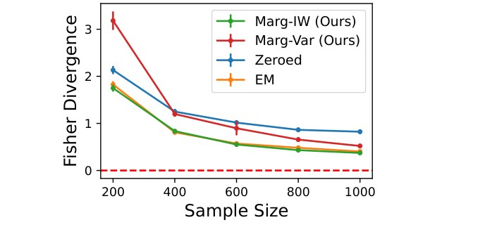
Figure 1: Average Fisher Divergence for Gaussian score estimates alongside 95% C.I.s Lower is better.
图 1:高斯 score 估计的平均 Fisher 散度及 95% 置信区间。越低越好。
Marg-IW and EM perform best with Marg-Var approaching asymptotically. We see the effect of Zeroed’s naive marginalisation as it does not converge, a phenomenon we discuss more in Appendix D.2. In Appendix B.1.1 we present the average mean and precision estimation error for this experiment. In Appendix B.1.2 we present the untruncated results and illustrate how the naive marginalisation poorly models strong relationship between dimensions 1 and 10.
Marg-IW 与 EM 表现最好,Marg-Var 渐近逼近。可见 Zeroed 的朴素边际化使其不收敛,附录 D.2 另有讨论。附录 B.1.1 给出本实验平均均值与精度估计误差;附录 B.1.2 给出未截断结果,并说明朴素边际化对第 1 与第 10 维之间的强相关建模很差。
5.1.2 Non-Gaussian Model
For this experiment we tested our parameter estimation for a an ICA inspired unnormalisable model of the form
5.1.2 非高斯模型
本实验测试受 ICA 启发的不可归一化模型上的参数估计,形式为
Here we parameterise our model identically with the aim of estimating . We vary the dimension of and plot the estimation error with a sample size of 1,000 and each coordinate missing independently with probability 0.5. The results are presented in Figure 2.
这里用相同参数化,目标是估计 。我们改变 的维数,在样本量 1000、各坐标以概率 0.5 独立缺失时画出估计误差。结果见图 2。
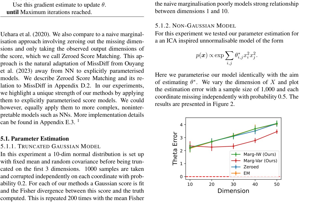
Figure 2: Average Fisher Divergence for Gaussian score estimates alongside 95% C.I.s. Lower is better.
图 2:高斯 score 估计的平均 Fisher 散度及 95% 置信区间。越低越好。
Our variational method (Marg-Var) consistently yields the lowest error. Moreover, as the dimensionality increases, the performance gap between Marg-Var and the other methods widens. This supports the notion that our approach is more accurately able to capture complex marginalisations than the competing approaches which fail as the dimension grows. We note that all other methods perform comparably with the performance of EM and Marg-IW being indistinguishable, a pattern we observe throughout our experiments. This similarity is unsurprising both approaches use self normalised importance weighting to approximate conditional expectations with respect to our current score estimate while being broadly motivated by fitting to the marginal scores. Nevertheless, the precise mechanism for this similarity remains unclear and warrants further exploration. Additional experiments exploring the effect of sample size and missingness probability on estimation accuracy are given in appendix B.1.3.
我们的变分方法(Marg-Var)始终给出最低误差。而且随着维数升高,Marg-Var 与其他方法的差距拉大。这支持如下看法:相对竞争方法,我们的做法更能准确刻画复杂边际化;后者随维数增长而失效。其余方法表现相近,EM 与 Marg-IW 几乎难分——这一模式贯穿实验。并不意外:二者都用自归一化重要性加权,相对当前 score 估计近似条件期望,且大体都由拟合边际 score 驱动。不过这种相似性的精确机制仍不清楚,值得继续探究。样本量与缺失概率对估计精度的影响见附录 B.1.3。
5.2 Gaussian Graphical Model Estimation
5.2 高斯图模型估计
Gaussian graphical models (GGM) are a popular way of modelling dependence between dimensions of data. Let us assume that the underlying data follows a Gaussian distribution with mean and precision . In this setting, a Bayesian network (BN) can represent the dependencies between the dimensions of with the (undirected) edges of the BN exactly being the non-zero off-diagonal entries of the precision, . Hence estimating the precision matrix P gives the BN. Score matching has been shown to be an effective way of achieving this with L1-regularisation on the off-diagonal of to push terms to (Lin et al., 2016; Yu et al., 2018). Decreasing the level of L1-regularisation then gives a range of classifiers with increasing True and False positive rates (TPR/FPR) as the level of regularisation decreases. Score matching can also be applied to truncated GGMs where we aim to learn the original BN but only observe the samples inside some truncated region.
高斯图模型(GGM)是刻画各维依赖的常用方式。假设底层数据服从均值 、精度 的高斯分布。此时贝叶斯网络(BN)可表示 各维依赖,且 BN 的(无向)边恰好对应精度 的非零非对角元。因此估计精度矩阵 即得到 BN。已有工作表明:对 非对角施加 L1 正则把项推向 0,score matching 能有效完成这一任务(Lin et al., 2016;Yu et al., 2018)。降低 L1 强度会得到一系列真阳性率/假阳性率(TPR/FPR)随正则减弱而上升的分类器。Score matching 也可用于截断 GGM:目标仍是学习原始 BN,但只观测截断区域内的样本。
We apply our methods to learn GGMs and truncated GGMs with missing data as well. We use varying levels of L1 regularisation on our objective via proximal stochastic gradient descent in our optimisation (Beck, 2017).
我们也把方法用于带缺失数据的 GGM 与截断 GGM。优化中通过近端随机梯度下降(Beck, 2017),在目标上施加不同强度的 L1 正则。
5.2.1 Star Shaped Truncated Graphical Model
Here we create a star shaped GGM in which one node has a high probability of being connected with each other node independently and all other connections have probability 0. We truncate the data along a random hyperplane such that 20% of the distribution lies outside of the truncation boundary. Each coordinate is then MCAR independently with the same probability. We run multiple experiments with this probability ranging from 0.2 to 0.9 and present the results in figure 3. As we can see here Marg-Var performs best with all other approaches performing comparably. For illustrative purposes, we plot individual ROC curves from this experiment in Appendix B.2.3.
5.2.1 星形截断图模型
构造星形 GGM:某一节点与其余各节点独立地以高概率相连,其余连接概率为 0。沿随机超平面截断数据,使分布约 20% 落在截断边界外。各坐标再以相同概率 MCAR 独立缺失。该概率从 0.2 扫到 0.9,结果见图 3。可见 Marg-Var 最好,其余方法相近。附录 B.2.3 给出本实验若干单独 ROC 曲线示意。
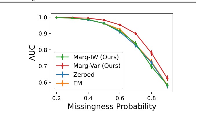
Figure 3: Mean AUC of star graph edge detection withg varying missingness alongside 95% C.I.s. Higher is better.
图 3:星图边检测平均 AUC 随缺失程度变化及 95% 置信区间。越高越好。
5.2.2 Unstructured Dense Graphical Model
Here we create a GGM by making each edge occur independently with probability 0.5. The rest of the experiment was constructed as before. Results are given in Figure 4.
5.2.2 无结构稠密图模型
这里令每条边以概率 0.5 独立出现来构造 GGM,其余设定同前。结果见图 4。
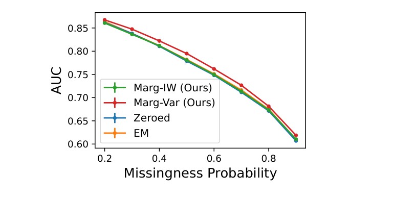
Figure 4: Mean AUC of dense graph edge detection with varying missingness alongside 95% C.I.s. Higher is better.
图 4:稠密图边检测平均 AUC 随缺失程度变化及 95% 置信区间。越高越好。
Again we can see that our variational approach performs best though not as clearly as in the previous example. We believe this to be because for more unstructured problems, naive marginalisation performs moderately well.
同样可见变分方法最好,但优势不如上一例清晰。我们认为:对更无结构的问题,朴素边际化也能达到中等水平。
5.2.3 Increasing Number of Stars
To explore this further, we construct and experiment where we vary the number of star centres (high degree nodes) while keeping the edge density constant. We present the results in Figure 5.
5.2.3 增加星心数量
为进一步探究,我们在保持边密度不变时改变星心(高度节点)数量。结果见图 5。
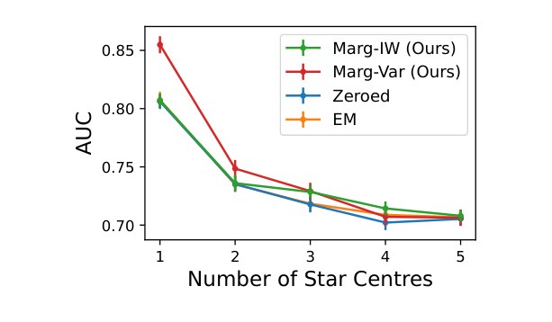
Figure 5: Mean AUC with 95% C.I.s for edge detection as number of star centres in graph varies. Higher is better.
图 5:边检测平均 AUC 及 95% 置信区间随图中星心数量变化。越高越好。
As we increase the number of star centres, Marg-Var no longer noticeably outperforms the other approaches. This is because as the number of stars increases, (i.e. the structure of the graph decreases) naive marginalisation is a better approximation. This is illustrated on the marginal precisions themselves in Appendix B.2.1.
随着星心增多,Marg-Var 不再明显优于其他方法。原因是星越多(即图结构越弱),朴素边际化近似越好。附录 B.2.1 在边际精度本身上对此有说明。
5.2.4 S&P 100
Here we took closing price data over 5 years for the 100 stocks in the S&P 100 with each stock being a dimension and each day being a sample. Gaussian graphical models with various levels of connectivity were then constructed using standard score matching on the fully observed data. The data was then artificially corrupted and each missing score matching approach applied. The AUC was then calculated for each method taking the GGM from fully observed score matching as the ground truth. More details given in appendix E.3.3. The results are shown in figure 6.
5.2.4 S&P 100
取 S&P 100 中 100 只股票五年收盘价:每只股票一维、每个交易日一个样本。先在完全观测数据上用标准 score matching 构造不同连通度的高斯图模型;再人工损坏数据,分别施加各缺失 score matching 方法;以完全观测 score matching 得到的 GGM 为真值计算 AUC。细节见附录 E.3.3。结果见图 6。
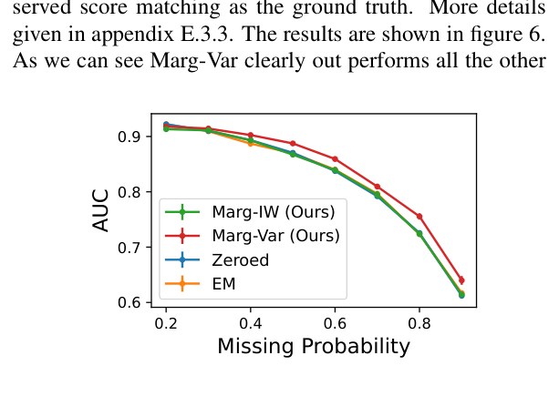
Figure 6: Mean AUC of various methods when compared to non-corrupted score matching with 95% confidence intervals on stocks in S&P 100. Higher is better.
图 6:相对未损坏 score matching,各方法在 S&P 100 股票上的平均 AUC 及 95% 置信区间。越高越好。
As we can see Marg-Var clearly out performs all the other approaches which appear to perform equivalently.
可见 Marg-Var 明显优于其余方法,后几者表现相近。
5.2.5 Yeast Data
Here data first introduced in Brem & Kruglyak (2005) is used consisting of readings of expression for 7086 genes/ORFs across 262 yeast segregants. Each gene represents a dimension with each segregant representing a sample. We subset the data to take the 106 genes present in at least 95% of the samples with the aim of learning the relationship between them.
5.2.5 酵母数据
使用 Brem & Kruglyak(2005)引入的数据:262 个酵母分离株上 7086 个基因/ORF 的表达读数。每个基因一维、每个分离株一个样本。我们取至少在 95% 样本中出现的 106 个基因子集,目标是学习它们之间的关系。
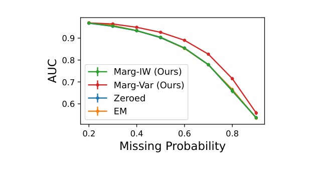
Figure 7: Mean AUC of various methods when compared to non-corrupted score matching with 95% confidence intervals on genetic yeast data. Higher is better.
图 7:相对未损坏 score matching,各方法在酵母基因数据上的平均 AUC 及 95% 置信区间。越高越好。
The same approach as the previous section is applied with the results shown in figure 7. Again Marg-Var clearly outperforms the other approaches which all perform comparably.
做法同上节,结果见图 7。同样 Marg-Var 明显更好,其余方法表现相近。
6 Conclusion
6 结论
To conclude, score matching is a versatile method whose applications at the heart of modern machine learning problems. In this work we have tackled the problem of adapting score matching to partially missing data. We have presented two separate but related approaches to this method, one using importance weighting and another using variational approximation. We have also provided extensions of these methods to truncated score matching, sliced and denoising score matching. For truncated score matching with our IW approach we have provided finite sample bounds on the accuracy of the estimated score in terms of the marginal truncated Fisher divergence.
总之,score matching 用途广泛,已深入现代机器学习核心问题。本文处理的是:如何把 score matching 适配到部分缺失数据。我们给出两种相关却不同的做法——重要性加权与变分近似——并把它们扩展到截断、切片与去噪 score matching。对截断 score matching 配 IW 方法,我们还给出了以边际截断 Fisher 散度度量的估计 score 精度的有限样本界。
We have provided several simulated and real world experiments demonstrating our methods’ efficacy for both parameter estimation and downstream GGM edge detection. We have shown the benefits and drawbacks of each approach with IW performing best in lower dimensional settings with less data and the variational approach performing best in more complicated higher dimensional settings.
我们用多项模拟与真实实验展示了方法在参数估计与下游 GGM 边检测上的效力,并说明各自利弊:IW 在较低维、数据较少时更强;变分方法在更复杂的高维设定更强。
There is, however still much work to be done in this area. From a theoretical perspective, while we have finite sample bound on the error of our loss, marginal nature of the loss makes it unclear exactly how this translates to parameter or general score model accuracy, leaving room for further theoretical exploration. From an implementation perspective, variational inference in the presence of missing data requires accounting for the randomness of “latent” and “observed” variables. The standard variational inference technique can be further refined to accommodate this setting. Finally, since our method is compatible with denoised score matching, it can naturally be extended to diffusion-based model. This paves the way for future work on applying our approach to generative modelling with diffusion processes in the presence of missing data.
该方向仍有大量工作。理论上,虽然我们对损失误差有有限样本界,但损失的边际性质使它与参数或一般 score 模型精度之间的对应并不清晰,有待继续理论探索。实现上,缺失数据下的变分推断需要同时处理「隐」与「观测」变量的随机性;标准变分技术还可针对该设定再 refinement。最后,由于方法兼容去噪 score matching,可自然扩展到基于扩散的模型,为缺失数据下的扩散生成建模铺路。
Acknowledgements
致谢
Josh Givens was supported by a PhD studentship from the EPSRC Centre for Doctoral Training in Computational Statistics and Data Science (COMPASS).
Josh Givens 由 EPSRC Centre for Doctoral Training in Computational Statistics and Data Science(COMPASS)博士生奖学金资助。
Impact Statement
影响声明
This paper presents work whose goal is to advance the field of Machine Learning. There are many potential societal consequences of our work, none which we feel must be specifically highlighted here.
本文旨在推进机器学习领域。工作可能带来多种社会影响,但我们认为无需在此特别强调。
References
参考文献
Bao et al. (2020) Bao, F., LI, C., Xu, K., Su, H., Zhu, J., and Zhang, B. Bi-level score matching for learning energy-based latent variable models. In Larochelle, H., Ranzato, M., Hadsell, R., Balcan, M., and Lin, H. (eds.), Advances in neural information processing systems , volume 33, pp. 18110–18122. Curran Associates, Inc., 2020. URL https://proceedings.neurips.cc/paper_files/paper/2020/file/d25a34b9c2a87db380ecd7f7115882ec-Paper.pdf .
Bao et al. (2021) Bao, F., Xu, K., Li, C., Hong, L., Zhu, J., and Zhang, B. Variational (gradient) estimate of the score function in energy-based latent variable models. In Meila, M. and Zhang, T. (eds.), Proceedings of the 38th international conference on machine learning , volume 139 of Proceedings of machine learning research , pp. 651–661. PMLR, July 2021. URL https://proceedings.mlr.press/v139/bao21b.html .
Beck (2017) Beck, A. The proximal gradient method. In First-order methods in optimization , pp. 269–329. Society for Industrial and Applied Mathematics, 2017. doi: 10.1137/1.9781611974997.ch10 . URL https://epubs.siam.org/doi/abs/10.1137/1.9781611974997.ch10 .
Brem & Kruglyak (2005) Brem, R. B. and Kruglyak, L. The landscape of genetic complexity across 5,700 gene expression traits in yeast. Proceedings of the National Academy of Sciences of the United States of America , 102(5):1572–1577, February 2005. ISSN 0027-8424 1091-6490. doi: 10.1073/pnas.0408709102 . Place: United States.
Burda et al. (2016) Burda, Y., Grosse, R. B., and Salakhutdinov, R. Importance weighted autoencoders. In Bengio, Y. and LeCun, Y. (eds.), 4th international conference on learning representations, ICLR 2016, san juan, puerto rico, may 2-4, 2016, conference track proceedings , 2016. URL http://arxiv.org/abs/1509.00519 . tex.bibsource: dblp computer science bibliography, https://dblp.org tex.timestamp: Thu, 25 Jul 2019 14:25:37 +0200.
Daras et al. (2023) Daras, G., Shah, K., Dagan, Y., Gollakota, A., Dimakis, A., and Klivans, A. Ambient diffusion: Learning clean distributions from corrupted data. In Thirty-seventh conference on neural information processing systems , 2023. URL https://openreview.net/forum?id=wBJBLy9kBY .
Fattahi & Sojoudi (2019) Fattahi, S. and Sojoudi, S. Graphical lasso and thresholding: Equivalence and closed-form solutions. Journal of Machine Learning Research , 20(10):1–44, 2019. URL http://jmlr.org/papers/v20/17-501.html .
Huang et al. (2021) Huang, C.-W., Lim, J. H., and Courville, A. C. A variational perspective on diffusion-based generative models and score matching. Advances in Neural Information Processing Systems , 34:22863–22876, 2021.
Hyvärinen (2005) Hyvärinen, A. Estimation of non-normalized statistical models by score matching. Journal of Machine Learning Research , 6(24):695–709, 2005.
Hyvärinen (2007) Hyvärinen, A. Some extensions of score matching. Computational Statistics & Data Analysis , 51(5):2499–2512, 2007. ISSN 0167-9473. doi: https://doi.org/10.1016/j.csda.2006.09.003 . URL https://www.sciencedirect.com/science/article/pii/S0167947306003264 .
Li et al. (2019a) Li, S. C.-X., Jiang, B., and Marlin, B. MisGAN: Learning from Incomplete Data with Generative Adversarial Networks. In International Conference on Learning Representations , 2019a. URL https://openreview.net/forum?id=S1lDV3RcKm .
Li et al. (2019b) Li, Z., Chen, Y., and Sommer, F. T. Learning energy-based models in high-dimensional spaces with multi-scale denoising score matching, 2019b. arXiv: 1910.07762 [stat.ML].
Li et al. (2023) Li, Z., Chen, Y., and Sommer, F. T. Learning energy-based models in high-dimensional spaces with multiscale denoising-score matching. Entropy. An International and Interdisciplinary Journal of Entropy and Information Studies , 25(10), 2023. ISSN 1099-4300. doi: 10.3390/e25101367 . URL https://www.mdpi.com/1099-4300/25/10/1367 . Number: 1367 tex.pubmedid: 37895489.
Lin et al. (2016) Lin, L., Drton, M., and Shojaie, A. Estimation of high-dimensional graphical models using regularized score matching. Electronic Journal of Statistics , 10(1):806 – 854, 2016. doi: 10.1214/16-EJS1126 . URL https://doi.org/10.1214/16-EJS1126 . Publisher: Institute of Mathematical Statistics and Bernoulli Society.
Liu & Wang (2017) Liu, Q. and Wang, D. Learning Deep Energy Models: Contrastive Divergence vs. Amortized MLE, July 2017. URL http://arxiv.org/abs/1707.00797 . arXiv:1707.00797 [cs, stat].
Liu et al. (2022) Liu, S., Kanamori, T., and Williams, D. J. Estimating density models with truncation boundaries using score matching. Journal of Machine Learning Research , 23(186):1–38, 2022. URL http://jmlr.org/papers/v23/21-0218.html .
Ouyang et al. (2023) Ouyang, Y., Xie, L., Li, C., and Cheng, G. MissDiff: Training diffusion models on tabular data with missing values. In ICML 2023 workshop on structured probabilistic inference & generative modeling , 2023. URL https://openreview.net/forum?id=S435pkeAdT .
Richardson et al. (2020) Richardson, T. W., Wu, W., Lin, L., Xu, B., and Bernal, E. A. MCFlow: Monte Carlo Flow Models for Data Imputation. In 2020 IEEE/CVF Conference on Computer Vision and Pattern Recognition (CVPR) , pp. 14193–14202, June 2020. doi: 10.1109/CVPR42600.2020.01421 . ISSN: 2575-7075.
Salimans & Ho (2021) Salimans, T. and Ho, J. Should EBMs model the energy or the score? In Energy based models workshop - ICLR 2021 , 2021. URL https://openreview.net/forum?id=9AS-TF2jRNb .
Sasaki et al. (2014) Sasaki, H., Hyvärinen, A., and Sugiyama, M. Clustering via mode seeking by direct estimation of the gradient of a log-density. In Calders, T., Esposito, F., Hüllermeier, E., and Meo, R. (eds.), Machine learning and knowledge discovery in databases , pp. 19–34, Berlin, Heidelberg, 2014. Springer Berlin Heidelberg. ISBN 978-3-662-44845-8.
Song & Ermon (2019) Song, Y. and Ermon, S. Generative Modeling by Estimating Gradients of the Data Distribution. In Advances in Neural Information Processing Systems , volume 32. Curran Associates, Inc., 2019.
Song et al. (2020) Song, Y., Garg, S., Shi, J., and Ermon, S. Sliced score matching: A scalable approach to density and score estimation. In Adams, R. P. and Gogate, V. (eds.), Proceedings of the 35th Uncertainty in Artificial Intelligence Conference , volume 115 of Proceedings of Machine Learning Research , pp. 574–584. PMLR, jul 2020.
Song et al. (2021a) Song, Y., Durkan, C., Murray, I., and Ermon, S. Maximum likelihood training of score-based diffusion models. Advances in Neural Information Processing Systems , 34:1415–1428, 2021a.
Song et al. (2021b) Song, Y., Sohl-Dickstein, J., Kingma, D. P., Kumar, A., Ermon, S., and Poole, B. Score-based generative modeling through stochastic differential equations. In International Conference on Learning Representations , 2021b.
Swersky et al. (2011) Swersky, K., Ranzato, M., Buchman, D., Freitas, N. D., and Marlin, B. M. On autoencoders and score matching for energy based models. In Proceedings of the 28th international conference on machine learning (ICML-11) , pp. 1201–1208, 2011.
Tashiro et al. (2021) Tashiro, Y., Song, J., Song, Y., and Ermon, S. CSDI: Conditional score-based diffusion models for probabilistic time series imputation. In Beygelzimer, A., Dauphin, Y., Liang, P., and Vaughan, J. W. (eds.), Advances in Neural Information Processing Systems , 2021.
Uehara et al. (2020) Uehara, M., Matsuda, T., and Kim, J. K. Imputation estimators for unnormalized models with missing data. In Chiappa, S. and Calandra, R. (eds.), Proceedings of the twenty third international conference on artificial intelligence and statistics , volume 108 of Proceedings of machine learning research , pp. 831–841. PMLR, August 2020. URL https://proceedings.mlr.press/v108/uehara20b.html .
Vincent (2011) Vincent, P. A connection between score matching and denoising autoencoders. Neural Computation , 23(7):1661–1674, 2011. doi: 10.1162/NECO_a_00142 .
Vértes & Sahani (2016) Vértes, E. and Sahani, M. Learning doubly intractable latent variable models via score matching. InSymposium on advances in approximate Bayesian inference (AABI) , 2016.
Yang & Lozano (2015) Yang, E. and Lozano, A. C. Robust gaussian graphical modeling with the trimmed graphical lasso. In Cortes, C., Lawrence, N., Lee, D., Sugiyama, M., and Garnett, R. (eds.), Advances in neural information processing systems , volume 28. Curran Associates, Inc., 2015. URL https://proceedings.neurips.cc/paper_files/paper/2015/file/3fb451ca2e89b3a13095b059d8705b15-Paper.pdf .
Yoon et al. (2018) Yoon, J., Jordon, J., and Schaar, M. Gain: Missing data imputation using generative adversarial nets. In International conference on machine learning , pp. 5689–5698, 2018. tex.organization: PMLR.
Yu et al. (2018) Yu, S., Drton, M., and Shojaie, A. Graphical models for non-negative data using generalized score matching. In Storkey, A. and Perez-Cruz, F. (eds.), Proceedings of the twenty-first international conference on artificial intelligence and statistics , volume 84 of Proceedings of machine learning research , pp. 1781–1790. PMLR, April 2018. URL https://proceedings.mlr.press/v84/yu18b.html .
Yu et al. (2022) Yu, S., Drton, M., and Shojaie, A. Generalized score matching for general domains. Information and Inference: A Journal of the IMA , 11(2):739–780, 2022.
Appendix A Additional Theoretical Results
附录 A 补充理论结果
Here we present some interesting results which we feel help further build up the landscape of our method but were unable to fit within the main body of the paper.
这里给出一些有助于进一步勾勒方法全貌、但未能放入正文的结果。
A.1 Additional Methods
A.1 补充方法
Firstly some additional adaptations of score matching. Most of these are relatively immediate adaptations following our framework for missing score matching although there are some important aspects and caveats which make them worth officially documenting. Missing and sliced score matching are introduced in detail in Appendix D.
首先是若干 score matching 的额外改编。多数是按缺失 score matching 框架的直接推广,但仍有若干要点与注意事项值得正式记录。缺失与切片 score matching 在附录 D 有更细介绍。
A.1.1 Truncated Score Matching
We have already presented truncated score matching in the paper however we present it in more details alongside its assumptions here.
A.1.1 截断 Score Matching
正文已介绍截断 score matching;这里给出更细形式及其假设。
Assumption A.1.
For any :
假设 A.1。
对任意 :
- • is connected, open and Lipschitz;
- • 连通、开且 Lipschitz;
- • ;
- • ;
- • are continuously differentiable and is twice continuously differentiable;
- • 连续可微, 二阶连续可微;
- • for any , and we have where is the normal vector to the boundary .
- • 对任意 与 ,有 其中 为边界 的法向量。
This now leads us to our proposition on the validity of our population objective.
据此我们得到总体目标有效性的命题。
Proposition A.2.
Suppose that assumptions 4.2 & A.1 hold. Then we have
命题 A.2。
设假设 4.2 与 A.1 成立。则
where is does not depend upon . As a direct result for a minimiser of we have that a.s..
其中 不依赖 。因此,若 是 的极小点,则几乎必然有 。
Proof.
Proof given in Appendix C.1.1 ∎
证明。
证明见附录 C.1.1 ∎
A.1.2 Missing Sliced Score Matching
For readers who are unfamiliar with sliced score matching we provide a brief introduction in Appendix D.3. For sliced score matching the only adaptations we need to make is to use our marginal scores and now alter our projection vectors to be over the appropriate subspace. Thus our objective becomes
A.1.2 缺失切片 Score Matching
不熟悉切片 score matching 的读者可先看附录 D.3 的简要介绍。对切片 score matching,只需改用边际 score,并把投影向量改到相应子空间。于是目标变为
where for any , is a RV on satisfying positive definite and .
其中对任意 , 为 上的随机变量,满足 正定且 。
To write this and it’s gradient in terms of the full score, we can again use Lemma 4.8.
要把该目标及其梯度写成完整 score 的形式,可再次使用引理 4.8。
This gives the following results
由此得到如下结果
Proposition A.3.
Proposition A.3.
where for any function ,
其中对任意函数 ,
and are w.r.t. with being w.r.t. .
且 取关于 , 取关于 。
Proof.
We first have that
证明。
首先有
The second results directly from applying Lemma 4.8 again alongside the chain rule.
第二个结果直接由再次应用引理 4.8 并结合链式法则得到。
∎
A.1.3 Missing Denoised Score Matching
As with sliced score matching the adaptation is relatively immediate however we do first need to make some further restrictions on our noising process. Specifically we require that for any , and we have .
A.1.3 缺失去噪 Score Matching
与切片 score matching 一样,改编相对直接,但需先对加噪过程再加一些限制。具体地,要求对任意 以及 ,有 。
In most practical implementations each coordinate is independently noised therefore satisfying this condition. We require this to allow us to easily write the marginal transition kernel for any given by . We then make our population objective
多数实际实现中各坐标独立加噪,因而满足该条件。我们需要它以便轻松写出任意 的边际转移核 。随后取总体目标为
We can again write this in terms of as we do in the following proposition
我们同样可把它写成 的形式,如下命题
Proposition A.4.
Proposition A.4.
where for any function ,
其中对任意函数 ,
and are w.r.t. with being w.r.t. .
且 取关于 , 取关于 。
Proof.
Using Lemma 4.8, we have that
证明。
由引理 4.8,有
A second application of the lemma then gives,
再次应用该引理则得到
∎
A.1.4 Missing not at Random Data
So far we have assumed that our data is missing completely at random so that . In other words, we could treat corrupted samples as though they were simply marginal samples and still perform valid inference. Often however, such an assumption is unrealistic and the probability of parts of a sample begin missing depends upon the sample itself. Generally this is split into two cases. Missing at Random (MAR) and Missing not at Random (MNAR). MAR data occurs when the probability of a coordinate being missing depends only upon other coordinates of the sample. This means that . In MNAR data we allow to depend upon as well meaning that an observations value determines its own probability of being missing.
A.1.4 非随机缺失数据
此前我们假设数据完全随机缺失,因而 。换言之,可把损坏样本当作单纯边际样本仍做有效推断。但该假设常常不现实:样本某部分缺失的概率可能依赖于样本本身。一般分为两类:随机缺失(MAR)与非随机缺失(MNAR)。MAR 指某坐标缺失概率只依赖样本其他坐标,即 。MNAR 则允许 也依赖 ,即观测值本身决定其缺失概率。
Here we will focus in the MNAR scenario and treat the MAR scenario as a special case of this. The core idea of this approach will be to work with a "joint" score rather than a marginal score. Before we do this we need to set-up our MNAR case. Specifically for define the event
这里聚焦 MNAR,并把 MAR 视为其特例。核心思路是使用「联合」score 而非边际 score。在此之前需先设定 MNAR 情形。具体地,对 定义事件
and define . Throughout we will assume each to be known. This is often an unrealistic assumption however this allows us the flexibility of having a method which is independent of how the are learned.
并定义 。全文假定每个 已知。这常常不现实,但使我们的方法可独立于 如何被学习。
To work with this MNAR data we need to define some adaptations of densities and score functions.
为处理 MNAR 数据,需对密度与 score 函数做一些改编。
Definition A.5.
with PDF and event define to be the "joint" density satisfying
定义 A.5。
对具有 pdf 的 与事件 ,定义 为满足下式的「联合」密度
for all .
对所有 。
From this and with our particular events we can redefine the missing score as,
由此并结合我们的具体事件,可把缺失 score 重新定义为
Remark A.6.
this missing score is not the same as the marginal score. We slightly abuse notation here using the same notation as we did for the marginal score. This is however reasonable as for the MCAR case the marginal score and the missing score are identical.
注 A.6。
该缺失 score 并不 等同于边际 score。这里略微滥用记号,沿用了边际 score 的同一写法。这仍合理:在 MCAR 情形,边际 score 与缺失 score 一致。
With this newly defined score, we can proceed similarly to the MCAR case and use the objective defined in (4) or (5) but with our new defined score. We now show a provide a similar justification for this approach as in the MCAR case but first need to introduce an additional assumption.
有了新定义的 score,可类似 MCAR 情形,使用 (4) 或 (5) 中定义的目标 ,但换用新 score。下面给出与 MCAR 类似的合理性论证;先引入额外假设。
Assumption A.7.
For each , a.s..
假设 A.7。
对每个 , 几乎必然严格为正。
Remark A.8.
We do not require every missingness pattern to have positive probability just that if a missingness pattern does have positive probability, it has positive probability for every possible underlying sample.
注 A.8。
我们并不要求每种缺失模式都有正概率;只要求在其发生时,条件概率 几乎必然为正,从而联合密度良定义。
This then leads us to our desired result.
由此得到我们想要的结果。
Proposition A.9.
Suppose with are in our MNAR set-up and assume that assumptions 4.2 & A.7 hold and that there exists $\theta^{}s_{\theta^{}}(X)=s_{\theta}(X)\tilde{\theta}L_{\marg}(\theta)\bm{s}_{\tilde{\theta}}(X)=\bm{s}(X)$ a.s..
命题 A.9。
设处于 MNAR 设定,并假定假设 4.2(经适当改写以适配新 score)与假设 A.7 成立。则最小化 (4)/(5) 中用新缺失 score 写出的目标,在相应正则条件下可辨识真 score。
The proof for this is similar to the MCAR case and is given in Appendix C.1.2.
证明与 MCAR 情形类似,见附录 C.1.2。
Now we have our objective we need to see how we can derive . Again we can do this similarly to the MCAR case. Let be our estimate of the unnormalised density then
有了目标后,还需说明如何得到 (以及其截断版本)以便在实践中优化。
As a result we can approximate our objective analogously to our approach for MCAR data.
因此可用与 MCAR 数据类似的方式近似我们的目标。
A.2 Finite Sample Bounds for Truncated Importance Weighted Score Matching
A.2 截断重要性加权 Score Matching 的有限样本界
To be able to prove finite sample bound results we first need to present some key definitions.
为证明有限样本界,先给出若干关键定义。
Definition A.10(Approximate Truncated Marginal Score Matching Objective).
For take our sample objective to be
定义 A.10(近似截断边际 Score Matching 目标)。
对 ,取样本目标为
with being our estimated marginal score from Definition 4.4.
其中 为定义 4.4 中的估计边际 score。
Additionally we define
此外定义
We now set-up the following assumptions
现给出如下假设
Assumption A.11.
There exists s.t. for all
假设 A.11。
存在 ,使得对所有
- • ,
- • ,
- •
Remark A.12.
It is this assumptions which restrict us from obtaining a similar result in the non-truncated case as it is unrealistic to have both and as .
注 A.12。
正是该假设使我们无法在非截断情形得到类似结果:既要 ,又要 (当 ),二者难以同时成立。
Assumption A.13.
For each we have that for any :
假设 A.13。
对每个 ,以及对任意 :
where are sub-Gaussian with parameters respectively for all .
其中对所有 , 分别为参数 的次高斯随机变量。
Remark A.14.
This assumption is immediately satisfied if is compact and are pointwise Lipschitz w.r.t. . Hence this assumption is slightly weaker than a uniformly lipschitz assumption
注 A.14。
若 紧且 关于 逐点 Lipschitz,则该假设立即成立。因此它略弱于一致 Lipschitz 假设。
We can now state our theorem
现在可以陈述我们的定理
Theorem A.15.
Assume that assumptions 4.2, A.1, A.11, A.13 hold and let be the minimisers of . If then for sufficiently large
定理 A.15。
设假设 4.2、A.1、A.11、A.13 成立,并令 为 的极小点。若 ,则当 充分大时
where depend upon , depends upon and depends upon , .
其中 依赖 , 依赖 , 依赖 与 。
Proof.
The proof for this alongside multiple intermediary results can be found in C.2 ∎
证明。
证明及若干中间结果见 C.2 ∎
Here we have shown convergence of our sample/approximate objective to the population objective. This combined with proposition A.2 which states that our population objective is minimised by the true score suggests that our approach does give valid inference for learning the score. A key limitation of our result is that to obtain convergence, we require . Furthermore, to obtain rate convergence we need to be of the same order as . As the computational complexity of our algorithm in , this suggests that to obtain our desired convergence to the population objective will have computational complexity.
这里我们证明了样本/近似目标向总体目标的收敛。再结合命题 A.2(总体目标由真 score 最小化),说明该方法对学习 score 给出有效推断。关键局限是:要收敛需 ;若要达到 速率, 还需与 同阶。由于计算成本随 增长,实践中常取较小 ,而理论保证则要求更大的 。
Remark A.16.
Our dependency on our Lipschitz constants only enters into the term with the associate sub-Gaussian parameters entering only into the .
注 A.16。
对 Lipschitz 常数的依赖只进入 项;相应的次高斯参数只进入 。
Remark A.17.
Dependence upon simply requires and bounded. This is achieved on a compact by and on a non-compact space by .
注 A.17。
对 的依赖只需 与 有界。在紧 上可由 实现;在非紧空间上可用 。
A.3 Relationship between IW and Variational objectives
A.3 IW 目标与变分目标的关系
Despite being derived quite differently from the marginal score matching objective. We show below that the two objectives are actually identical in some cases. Specifically, when the IW density doesn’t depend upon the observed data , we can treat the importance weighted approach as an importance weighting approximation of the gradient estimate in (10). We demonstrate this through the two results below
尽管推导路径与边际 score matching 目标很不同,我们下面说明二者在某些情形实际相同。具体地,当 IW 密度 不依赖观测数据 时,可把重要性加权做法视为对 (10) 中梯度估计的重要性加权近似。下面两个结果说明这一点。
Lemma A.18.
For some density which generates IID samples let
引理 A.18。
对生成 IID 样本 的某密度 ,令
Then
则
where represents the gradient w.r.t. or . In other words, we can take importance weights first then gradients (LHS) or gradients and then importance weights (RHS).
其中 表示关于 或 的梯度。换言之,可先做重要性加权再求梯度(左边),或先求梯度再做重要性加权(右边)。
Proof.
Proof given in Section C.4. ∎
证明。
证明见第 C.4 节。∎
Corollary A.19.
We have that
推论 A.19。
我们有
Proof.
Proof given in Section C.4. ∎
证明。
证明见第 C.4 节。∎
A.4 Exploring the Marginal Fisher Divergence for Normal Distributions
A.4 正态分布下边际 Fisher 散度的探讨
While intuitively the Fisher divergences of the marginal distributions should act as effective proxies for the Fisher divergence for the fully observed distributions, we would like to be able to examine the relationship between the two more explicitly. We do know that marginal Fisher divergences will be zero when then fully observed distributions equivalent however here we give a more detailed examination in the case of normal distributions.
直观上,边际分布的 Fisher 散度应能有效代理完全观测分布的 Fisher 散度;我们希望更显式地考察二者关系。已知当完全观测分布等价时边际 Fisher 散度为零;这里在正态分布情形给出更细致的分析。
Suppose that
设
with a constant w.r.t. . We then have that
其中 为不依赖 的常数。于是
If we suppose that our unnormalised density/score model is of the form
若假定未归一化密度/score 模型形如
Then with the marginal Fisher taken to be
则取边际 Fisher 为
where here for each , are the true marginal scores. Using properties of the normal distribution and the Schur complement we know that the precision of is given by
其中对每个 , 为真边际 score。利用正态分布性质与 Schur 补可知, 的精度为
Plugging this in we get
代入得到
This shows why naive marginalisation by zeroing out missing coordinates of our score would not work as in this case the Fisher divergence would be given by
这说明为何把缺失坐标的 score 置零做朴素边际化行不通:此时 Fisher 散度将变为
which encourages to be close to for all meaning it will not give us the true density.
它鼓励对所有 使 接近 ,因而得不到真密度。
A.5 Variational Pseudo-loss
A.5 变分伪损失
When using (10) it is helpful to be able to view it as the gradient of some pseudo-loss allowing it to plug into a more standard ML framework where we calculate the loss, take the gradient w.r.t. our parameter using auto-differentiation, and update our parameter estimate based on this. The below result show how we can do this by creating a loss with certain instances of our parameter detached from the computational graph.
使用 (10) 时,最好能把它看成某个伪损失的梯度,从而接入更标准的机器学习流程:计算损失、用自动微分对参数求梯度、再据此更新参数估计。下述结果表明:可通过构造损失、并把参数的某些出现从计算图中分离(detach)来实现。
Proposition A.20.
Let
命题 A.20。
令
where are w.r.t. Then
其中 取关于 。则
Proof.
This just follows directly from the exchangeability of expectations and gradients (when the gradient is w.r.t. something independent of the expectation distribution.) ∎
证明。
这直接来自期望与梯度的可交换性(当梯度所对的量独立于期望所对的分布时)。∎
Hence we can use this loss (by replacing all instances of with and then detaching them from the computation graph) to treat our problem as a standard gradient descent problem.
因此可用该损失(把所有 换成 并从计算图分离)把问题当作标准梯度下降。
Note that while we can treat this like a loss for our optimisation, our intent is not actually to minimise it. The estimated form of the loss is given in the proof of Corollary 4.9 which is given in C.3 but we state it again explicitly here for convenience.
注意:虽可在优化中把它当损失用,我们的意图并非真正最小化它。损失的估计形式见推论 4.9 的证明(C.3);为方便这里再显式写出。
Appendix B Additional Experimental Results
附录 B 补充实验结果
Here we present some additional experimental results not in the main body of the paper.
这里给出正文未收录的若干补充实验结果。
B.1 Parameter Estimation
B.1 参数估计
B.1.1 Truncated Gaussian Model
Here we present the accompanying mean and precision error results for Gaussian model estimation experiment presented in Section 5.1.1. These results are presented in Figure 8.
B.1.1 截断高斯模型
这里给出第 5.1.1 节高斯模型估计实验配套的均值与精度误差结果,见图 8。
(a) Average error in estimation of the Mean (L2 norm).
(a) 均值估计平均误差(L2 范数)。
B.1.2 Untruncated Gaussian Model
Here we present the untruncated version of the experiment presented in the main paper. Details of the distribution are the same as presented in Appendix E.3 but without the truncation.
B.1.2 未截断高斯模型
这里给出正文实验的未截断版本。分布设定同附录 E.3,但不做截断。
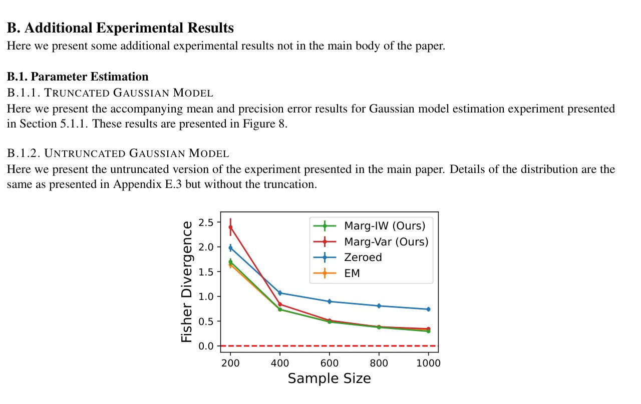
Figure 9: Average Fisher Divergence with 95% C.I.s for various approaches. Lower is better.
图 9:各方法平均 Fisher 散度及 95% 置信区间。越低越好。
As we can see we obtains similar results here as in the truncated case.
可见结果与截断情形类似。
We also illustrate what the true covariance and precision matrix look like for this example alongside the naive marginalisation in order to highlight where Zeroed Score Matching goes wrong.
我们还展示本例真协方差与精度矩阵,以及朴素边际化结果,以说明 Zeroed Score Matching 错在何处。
In Figure 10 we can see the covariance and precision of a sample distribution where we can clearly see the strong dependence of dimensions 1 and 10 relative to the others.
图 10 给出某样本分布的协方差与精度,可清楚看到第 1 与第 10 维相对其他维的强依赖。
(a) Covariance
(a) 协方差
(a) Naive Marginalisation
(a) 朴素边际化
In Figure 11 we can see the naive and true marginal precisions when dimension 1 is missing. For this plot the values have been cube-rooted in order to emphasize the difference between zero and non-zero entries. Here we can see that the naive marginalisation wouldn’t capture the dependence between dimension 10 and the other dimensions that gets introduced when dimension 1 is removed. This means that a naive marginalisation would assume that dimension 10 must have a direct dependence on dimensions 2-9 even when that is not true. Interestingly, the rest of the marginalisation seems very similar suggesting that in some potentially less structured cases, naive marginalisation can provide a semi-reasonable approximation. This supports the results we see in our GGM estimation where highly structured graphs like star graphs are much more affected naive marginalisation than unstructured graphs.
图 11 给出缺失第 1 维时的朴素与真边际精度。为突出零与非零条目差异,图中数值做了立方根变换。可见朴素边际化抓不住去掉第 1 维后第 10 维与其他维之间新出现的依赖,因而会误以为第 10 维必须与第 2–9 维有直接依赖,即便事实并非如此。有趣的是,其余边际化结果看起来仍相当接近。
B.1.3 Non-Gaussian Estimation
Here we present further experiments exploring the non-Gaussian model presented in Section 5.1.2. Here we fix the dimension as 10. In Figure 12(a) we fix the missing probability as 0.5 and vary the sample size. In Figure 12(b) we fix the sample size as 1000 and vary the missing probability.
B.1.3 非高斯估计
这里给出第 5.1.2 节非高斯模型的进一步实验。维数固定为 10。图 12(a) 固定缺失概率 0.5、改变样本量;图 12(b) 固定样本量 1000、改变缺失概率。
(a) Varying sample size with missing probability 0.5 and dimension 10.
(a) 缺失概率 0.5、维数 10 时改变样本量。
From Figure 12(a) we see that both EM and Marg-IW have the smallest estimation error for larger sample sizes. Zeroed Score Matching has the largest estimation error due to its inability to appropriately marginalise the distribution. In Figure 12(b), we observe that Marg-Var has the smallest estimation error with its performance convergence to that of Marg-IW and EM as the missing probability increases.
由图 12(a),大样本时 EM 与 Marg-IW 估计误差最小。Zeroed Score Matching 因无法恰当边际化而误差最大。图 12(b) 中 Marg-Var 误差最小;随缺失概率升高,其表现向 Marg-IW 与 EM 收敛。
B.2 GGM Estimation
B.2 GGM 估计
B.2.1 Varying Number of Star Centres
Here we present illustrations of the marginalisations for our star-shaped graphs with 1 node and then 5 nodes both with the same edge density.
B.2.1 改变星心数量
这里展示边密度相同、星心分别为 1 与 5 的星形图的边际化示意。
In Figure 13 we show the covariance, precision, marginal covariance, and marginal precision for a star graph with 1 centre where the marginal terms are with dimension 1 removed. As we can see clearly the only meaningful structure left in the graph after marginalisation are in the negative precision terms which the model naive marginalisation fails to capture.
图 13 给出单星心星图的协方差、精度、边际协方差与边际精度(边际项去掉第 1 维)。可见边际化后图中仅存的有意义结构落在负精度项上,而模型的朴素边际化未能捕捉。
(a) Covariance
(a) 协方差
In Figure 14 we show the same thing for the case of a star graph with 5 centres. As we can see in the 5 centre case, the naive marginalisation picks up most of the structure as there are fewer negative terms which it ignores and also lots of additional positive terms which it does successfully pick up.
图 14 给出五星心情形的同样内容。可见五星心时朴素边际化能抓住大部分结构:它忽略的负项更少,同时成功捕获许多额外正项。
(a) Covariance
(a) 协方差
B.2.2 Varying Number of Dimensions
Here we use our same star-shaped GGM as in the main paper but with a varying number of dimensions. Throughout 1,000 samples are used and each coordinate is missing independently with probability 0.7. Results are presented in Figure 15.
B.2.2 改变维数
沿用正文星形 GGM,但改变维数。全程用 1000 个样本,各坐标以概率 0.7 独立缺失。结果见图 15。
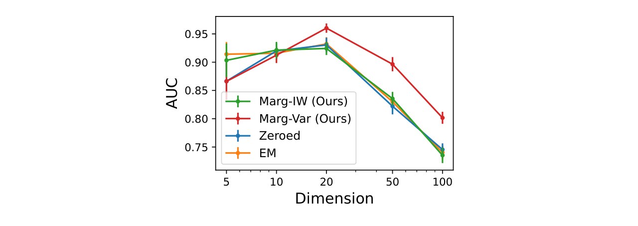
Figure 15: Mean AUC of various methods for edge detection of star-shaped GGM as we increase the dimension presented alongside 95% confidence intervals.
图 15:星形 GGM 边检测平均 AUC 随维数增加的变化及 95% 置信区间。
As we can see, for higher dimensions the variational approach clearly performs best however at lower dimensions the other approach catch up and even overtake it. This is because at lower dimensions, IW can effectively model the marginalisation of the score and so the more complicated variational approach is not required.
可见高维时变分方法明显最好;低维时其他方法赶上甚至反超。因为低维时 IW 已能有效建模 score 的边际化,不必再上更复杂的变分方法。
B.2.3 Individual ROC Curves
Here we present individual ROC curves from Section 5.2.1 with a missing probability of 0.5. Here we specifically present the ROC curves from the first 4 runs out of the 50 performed for the experiment. These ROC curves are displayed in Figure 16. We observe that Marg-Var has consistently the best ROC curves of any of the methods.
B.2.3 单条 ROC 曲线
这里给出第 5.2.1 节在缺失概率 0.5 时的单条 ROC。具体展示该实验 50 次运行中前 4 次的 ROC,见图 16。可观察到 Marg-Var 的 ROC 始终优于其他方法。
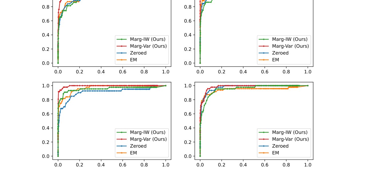
Figure 16: ROC Curves in 4 separate runs for GGM estimation of a model truncated normal distribution with a star-shaped Precision matrix.
图 16:截断正态分布、星形精度矩阵的 GGM 估计在 4 次独立运行中的 ROC 曲线。
Appendix C Additional Proofs
附录 C 补充证明
C.1 Marginal Score Matching Objectives
C.1 边际 Score Matching 目标
proof of Proposition 4.3.
For the first claim we have that
命题 4.3 的证明。
对第一个断言,有
justifying our first claim. Hence if minimised our objective then it minimises
从而证明第一个断言。因此若 最小化我们的目标,则它也最小化
As there exists a "true" we know that this objective is minimised at and so we must have a.s. for all . By our assumption this then gives a.s. . ∎
由于存在「真」,该目标在 0 处取得最小,故对所有 几乎必然有 。再由假设得几乎必然 。∎
Proof of Proposition A.2.
We mostly use (Liu et al., 2022). We firstly have that
命题 A.2 的证明。
我们主要依据 Liu et al.(2022)。首先有
Now we have that
接着有
where is given by Green’s Theorem and is given by our limiting condition. Plugging this back into our original result gives
其中 (a) 由 Green 定理给出,(b) 由极限条件给出。代回原结果得
From our conditions we also know that is a minimiser of hence by our conditions it is the unique minimiser. Therefore is the unique minimiser of ∎
由条件亦知 是 的极小点,且在我们的条件下唯一,故 也是 的唯一极小点。∎
Proof of Proposition A.9.
Firstly we have that
命题 A.9 的证明。
首先有
where does not depend upon . Examining the second term closer we see that
其中 不依赖 。更仔细看第二项,有
Hence we have
于是
Hence, just as in Proposition 4.3 this is minimised when
因此与命题 4.3 一样,当
a.s. for all . We then have that for any
对所有 几乎必然成立时取得最小。进而对任意
∎
C.2 Finite Sample Bound Proofs
C.2 有限样本界证明
Here we give some key results alongside their proof to allow us to obtains finite sample bounds for truncated score matching. This first result is what really underpins our approach.
这里给出若干关键结果及其证明,以便得到截断 score matching 的有限样本界。第一个结果是我们方法真正的支撑。
Proposition C.1.
Let be a compact metric space and for any denote the -covering number of by . Now define random functions for all (with deterministic) such that for any
命题 C.1。
设 为紧度量空间,对任意 用 表示 的 -覆盖数。现对所有 ( 确定性)定义随机函数 ,使得对任意
If we additionally assume that Lipschitz with constants respectively then we have then
若再假定 分别以常数 Lipschitz,则
Proof.
Let be an cover of then we have that
证明。
令 为 的 覆盖,则
Therefore we have the following relationship between events:
于是事件之间有如下关系:
This therefore gives
因此得到
∎
Remark C.2.
This result does not require too be deterministic. A feature that we will be exploiting later on.
注 C.2。
该结果不要求 确定性;后文将用到这一性质。
To be able to say meaningful statements about our Lipschitz bounds for our proof, it will also be helpful to make subgaussian statements about nested sums. We give to results to enable this now
为在证明中对 Lipschitz 界作有意义陈述,还需要对嵌套和给出次高斯结论。下面给出两个结果。
Lemma C.3.
Let be independent RVs and define a function . Now suppose that for any , is sub-Gaussian with parameter . We then have that is sub-Gaussian with parameter
引理 C.3。
设 独立,并定义 。若对任意 , 为参数 的次高斯,则 亦为参数 的次高斯。
Proof.
As sub-Gaussian we have that for any
证明。
因 次高斯,对任意 有
Our aim is to then use this to bound
目标是据此界住
We first have that which in turn gives
首先 ,从而
∎
Lemma C.4.
Let be independent RVs on spaces and s.t. for any and are sub-Gaussian with parameters respectively. Let and be IID copies of respectively then
引理 C.4。
设 为 上独立随机变量, 使得对任意 , 与 分别为参数 的次高斯。令 与 分别为 的 IID 副本,则
Proof.
Again let , We aim to bound as well as
证明。
再令 ,目标是界住 以及 。
For we have that
对 有
Therefore we have that
因此
Additionally from Lemma C.3 we have that is sub-Gaussian with parameter giving us that
此外由引理 C.3, 为参数 的次高斯,故
Hence combining these we get
合并二者得到
∎
To proceed we define the intermediary step between the population objective and the sample objective this is
为继续,定义总体目标与样本目标之间的中间量,即
Proposition C.5.
For let be IID copies of and assume that . For and , with define RVs by
命题 C.5。
对 ,令 为 的 IID 副本,并假定 。对 与 (),定义随机变量 为
Suppose that the following hold for all
设对所有 成立
- •
- •
- •
- •
- •
Then we have that
则
with depending upon .
其中 依赖 。
Proof.
First define
证明。
先定义
Using the definition of the marginal and estimated marginal score we then have that
利用边际与估计边际 score 的定义,有
We can therefore write write as
于是可把 写成
Now if we define the events
若定义事件
then we have that
则有
Using standard Hoeffding bounds for and union bounds in conjunction with Hoeffding bounds for we get that
对 用标准 Hoeffding 界,并对 用并界结合 Hoeffding,得到
Hence
故
∎
proof of Theorem A.15.
Our strategy will be as follows:
定理 A.15 的证明。
策略如下:
- • Use our bound on from Proposition C.5 to bound .
- • 用命题 C.5 对 的界,去界住 。
- • Use a covering number argument alongside Lemma C.4 to bound .
- • 用覆盖数论证并结合引理 C.4,界住 。
- • Use a similar approach to bound .
- • 用类似方法界住 。
- • Combine these to bound
- • 合并上述结果,界住
For the first step we have that
第一步有
where
其中
We now try and derive a Lipschitz constant for both and . Define by
现在试图为 与 导出 Lipschitz 常数。定义 为
Then we have that For we have
则对 有
similarly we have
类似地有
Using an identical argument to Proposition C.1 can get the following bound for any :
用与命题 C.1 相同的论证,对任意 可得
Hence we now need to bound and . We know that both of these terms converge to . To obtain rates on this convergence we make sub-Gaussian statements about . Specifically for we have that is sub-Gaussian with parameter
因此还需界住 与 。二者都收敛到 。为得到收敛速率,对 作次高斯陈述。具体地,对 , 为参数如下的次高斯
We can therefore immediately bound using Lemma C.3 and Hoeffding bounds to get
于是可立即用引理 C.3 与 Hoeffding 界住 ,得到
where . To bound we can use Lemma C.4 to get
其中 。对 可用引理 C.4 得到
with define identically to with replaced with and replaced with . As a result we get that
其中 的定义与 相同,只是把 换成 、把 换成 。于是
Now we have the bound on . We aim to bound . To that end we have
至此已有 的界。我们还要界住 。为此有
a.s. and so we can use Hoeffding bounds to get
几乎必然成立,因而可用 Hoeffding 界得到
Again using an argument similar to Proposition C.1 we have for any
再次用类似命题 C.1 的论证,对任意 有
Combining these two results gives that for any
合并二者,对任意 有
Take and so that for sufficiently large and . Plugging this into (22) gives
取 、,则当 充分大时 ,。代入 (22) 得
Now if we take each of these terms to be equal to gives for sufficiently large
再令各项等于 ,则当 充分大时
where , . As there exists a minimiser of we now have that
其中 ,。由于存在 的极小点 ,于是
Finally we know that and under a correctly specified model . Therefore we have that
最后知 ,且在模型正确设定时 。因此
and so we have our result simply replacing with . ∎
把 换成 即得结论。∎
C.3 Gradient First Proofs
C.3 先求梯度的证明
Proof of Lemma 4.8.
First we have that for any ,
引理 4.8 的证明。
首先,对任意 ,
Taking expectations on both side w.r.t. proves equation (8).
两边关于 取期望即得式 (8)。
For (9) we have again for any ,
对 (9),同样对任意 ,
Where again here represents the gradient w.r.t. either or . We can again take expectations on both sides w.r.t. to get our result. ∎
此处 仍表示关于 或 的梯度。再关于 取期望即得结果。∎
Proof of Corollary 4.9.
First define
推论 4.9 的证明。
先定义
so that . Then using our two score identities, (8) & (9) we can re-write as
使得 。再利用两条 score 恒等式 (8) 与 (9),可把 改写为
\displaystyle L_{\marg}(\theta;\bm{x}) \\ \displaystyle=\sum_{j\in\lambda}\mathbb{E}^{\prime}[\bm{s}_{\theta}(\bm{x}_{\lambda},X^{\prime}_{-\lambda})_{j}]^{2}+2\partial_{j}\mathbb{E}^{\prime}[\bm{s}_{\theta}(\bm{x}_{\lambda},X^{\prime}_{-\lambda})_{j}]\quad\text{by \eqref{eq:mcmc_score_equiv}} \\ \displaystyle=\sum_{j\in\lambda}\mathbb{E}^{\prime}[\bm{s}_{\theta}(\bm{x}_{\lambda},X^{\prime}_{-\lambda})_{j}]^{2}+\mathbb{E}^{\prime}[\partial_{j}\bm{s}_{\theta}(\bm{x}_{\lambda},X^{\prime}_{-\lambda})_{j}]+\var(s_{\theta}(\bm{x}_{\lambda},X^{\prime}_{-\lambda})_{j})\quad\text{by \eqref{eq:mcmc_gradscore_equiv}} \\ \displaystyle=\sum_{j\in\lambda}-\mathbb{E}^{\prime}[s_{\theta}(\bm{x}_{\lambda},X^{\prime}_{-\lambda})_{j}]^{2}+2\mathbb{E}^{\prime}[s_{\theta}(\bm{x}_{\lambda},X^{\prime}_{-\lambda})_{j}^{2}]+2\mathbb{E}^{\prime}[\partial_{i}s_{\theta}(\bm{x}_{\lambda},x_{-\lambda})_{j}]
Where all expectations are w.r.t. Now using the fact that
其中所有期望取关于 。再利用
and using (9) again on each term of the above gives followed by taking expectations w.r.t. gives the result. ∎
并对上式各项再次使用 (9),再关于 取期望,即得结果。∎
Proof of Corollary 4.11.
Now using Lemma 4.8, we know that this can be re-written as
推论 4.11 的证明。
由引理 4.8,可知它可改写为
Now taking gradient w.r.t. we get
再关于 求梯度得
∎
C.4 IW and Gradient First Relationships
C.4 IW 与先求梯度做法的关系
Proof of Lemma A.18.
We first have that,
引理 A.18 的证明。
首先有
Where the penultimate result uses the fact that
其中倒数第二个结果用到
Additionally,
此外,
For the second term we can again use to write this as
对第二项,可再次用 写成
The first term we can write as
第一项可写成
Combining these 2 gives our desired results. ∎
合并二者即得所需结果。∎
Proof of Corollary A.19.
The exact same arguments give us the second result but with the importance weighting identities (19) and (20) replacing (8) & (9). ∎
推论 A.19 的证明。
完全相同的论证给出第二个结果,只需用重要性加权恒等式 (19)、(20) 替换 (8)、(9)。∎
Appendix D Additional Score Matching Details & Extensions
附录 D Score Matching 补充细节与扩展
In this section we give some additional details on score matching and introduce some pre-existing score matching extensions and methods. For some of these approach we can adapt our method to work with them while others act as comparison points for our approach.
本节补充 score matching 细节,并介绍若干已有扩展与方法。对其中一些做法,我们的方法可适配;另一些则作为比较基准。
D.1 Classical Score Matching
D.1 经典 Score Matching
The assumptions for the classical score matching result presented in (1)
(1) 中经典 score matching 结果所需假设为
Assumption D.1.
For
假设 D.1。
对
(a) The pdf is differentiable w.r.t. ;
(a) pdf 关于 可微;
(b) Our score estimating function is differentiable w.r.t. ;
(b) score 估计函数 关于 可微;
(c) ,;
(c) ,;
(d) whenever .
(d) 每当 时,。
D.2 Zeroed Score Matching and MissDiff
D.2 Zeroed Score Matching 与 MissDiff
In this section we take to be the vector in with if and otherwise and then take to be the RV equivalent.
本节取 为 中满足:若 则 ,否则为 0 的向量;并取 为相应随机变量。
MissDiff is a generative modelling technique that aims to learn generative models from corrupted tabular data using diffusion models with denoising score matching. Throughout their method is assumed to be a neural network. The core idea is to replace the standard score matching objective with
MissDiff 是一种生成建模技术,目标是用带去噪 score matching 的扩散模型,从损坏表格数据学习生成模型。其方法中假定 为神经网络。核心想法是把标准 score matching 目标换成
Essentially, missing values are zero imputed and then the score is tested only on output dimensions whose input dimensions are non-missing. The idea of this approach is that it trains to approximate the true marginal score which in turn encourages to approximate the full score .
本质上,缺失值用零填补,然后只在输入维非缺失的那些输出维上检验 score。思路是训练 去逼近真边际 score ,从而促使 逼近完整 score 。
For comparison purposes, we adapt this in two ways to create Zeroed Score Matching. Firstly we change the objective to standard score matching and secondly we no longer require to be a neural network. Thus our adapted version of the MissDiff objective is
为便于比较,我们从两方面改编得到 Zeroed Score Matching:一是把目标改回标准 score matching;二是不再要求 为神经网络。于是改编后的 MissDiff 目标为
The key issue with this approach is that with no longer necessarily a neural network it is not reasonable (or indeed even possible) for to model both the joint and marginal scores. In other words we cannot expect both and making it a naive marginalisation method for the score.
关键问题是:当 不必是神经网络时,期望它同时建模联合与边际 score 并不合理(甚至不可能)。换言之,不能同时期望 与 ,因而它只是对 score 的朴素边际化。
We can give a brief example with a multidimensional normal distribution. Supposed that with . Then the score is which we would model with . Under the Zeroed scheme, we would take the marginal score to be
可用多维正态分布作简例。设 ,。则 score 为 ,我们用 建模。在 Zeroed 方案下,会把边际 score 取为
However we know that if with then and so we should take
但若 且 ,则 ,因而应取
and crucially, unless .
关键是:除非 ,否则 。
We illustrate this for our simulated experimental settings in Appendices B.1.2 & B.2.1.
附录 B.1.2 与 B.2.1 在我们的模拟实验设定中说明了这一点。
We also explore the implications of this for the marginal Fisher divergence for the normal in Appendix A.4.
我们也在附录 A.4 探讨了这对正态边际 Fisher 散度的含义。
D.3 Sliced Score Matching
D.3 切片 Score Matching
One issue with score matching is that is computationally expensive to compute for large . A solution to this was proposed in Song et al. (2020) where, instead of testing the full score 1-dimensional projections/slices are tested instead. This is done by introducing another RV on satisfying and positive semi-definite.
Score matching 的一个问题是:对大 , 计算昂贵。Song et al.(2020)提出一种解法:不再检验完整 score,而检验其一维投影/切片。做法是引入另一个随机变量 ,取值于 ,满足 且 半正定。
The original objective is then
原目标于是为
Which then leads to the following equivalence
由此得到如下等价形式
which is less computationally expensive w.r.t. and can be approximated with samples of and . For the proof of this results and the precise conditions see Song et al. (2020).
它对 的计算更省,并可用 与 的样本近似。证明与精确条件见 Song et al.(2020)。
D.4 Denoised Score matching
D.4 去噪 Score Matching
Denoised score matching is another adaptation which removes the need to takes derivatives of the score all together (Vincent, 2011). As we will see later on it is also the method used most prominently in diffusion processes.
去噪 score matching 是另一种改编,完全不必对 score 再求导(Vincent, 2011)。后文可见,它也是扩散过程中最常用的做法。
In denoising score matching we construct a collection of RVs with and . We assume that the noise grows sufficiently so that is approximately an Isotropic Gaussian. The aim is now to estimate where is the PDF of . The denoising score matching objective is then.
在去噪 score matching 中,我们构造一族随机变量 ,满足 且 。假定噪声 增长到使 近似各向同性高斯。目标是估计 ,其中 为 的 pdf。去噪 score matching 目标为
where here is treated as random and uniformly distributed on , is the transition kernel from to and is a self-specified weighting function over time. Due to our choice of noising process, .
这里把 视为在 上均匀的随机变量, 为从 到 的转移核, 为自选的时间权重。由于加噪过程的选取,。
Remark D.2.
Convention is to up-weight larger values of as earlier parts of the reverse diffusion process (hence later parts of the original diffusion process) are seen as the most complex and where most of the data’s structure is learned.
注 D.2。
惯例是给较大的 更高权重:反向扩散过程的较早阶段(亦即原扩散过程的较晚阶段)被视为最复杂,也是数据主要结构被学习之处。
Our estimate is thus
于是我们的估计为
where are sampled uniformly from .
其中 从 均匀抽样。
Remark D.3.
Originally denoising score matching was proposed for a single fixed however for the purpose of generative modelling and annealed Langevin dynamics, multiple noise levels or even a continuous noising processes are used.
注 D.3。
去噪 score matching 最初针对单一固定 提出;但面向生成建模与退火 Langevin 动力学时,会使用多个噪声水平,甚至连续加噪过程。
Appendix E Additional Details
附录 E 补充细节
E.1 Objectives
E.1 目标函数
E.1.1 Marginal IW Score Matching Objective
Let be IID copies of with known PDF . Our full sample objective is given by
E.1.1 边际 IW Score Matching 目标
令 为具有已知 pdf 的 的 IID 副本。完整样本目标为
E.1.2 Marginal Truncated IW Score Matching
Our full sample objective for truncated IW missing score matching is given by
E.1.2 边际截断 IW Score Matching
截断 IW 缺失 score matching 的完整样本目标为
E.2 Variational Modelling Details
E.2 变分建模细节
For our purposes our variational model has to able able to model for any value of . For our model we take .
对我们而言,变分模型 必须能对任意 建模 。我们取 。
Hence we require to take in any subset of coordinates and output the complementing coordinates We achieve this by creating , a -dim in to -dim out Neural Network with 2 hidden layers of 200 nodes as per Burda et al. (2016). For the input we replace with the zero filled version inline with the approach taken in MissDiff (Ouyang et al., 2023). That is if and is otherwise. As output we then simply take the appropriate coordinates. We can write this more succinctly as
因此要求 能接受任意坐标子集并输出互补坐标。做法是构造 :按 Burda et al.(2016)用两层各 200 节点的隐层,做成 维入、 维出的神经网络。输入上把 换成与 MissDiff(Ouyang et al., 2023)一致的零填充版本 ,即若 则 ,否则为 。输出则只取相应坐标。更简洁地写成
We also experimented with making a dim input NN and taking
我们也试过让 成为 维输入网络,并取
where is the d-dimensional binary mask for the corruption similarly to GAIN (Yoon et al., 2018) however this did not seem to provide any advantage. We also experimented with making depend upon however we found this made training much more unstable.
其中 为类似 GAIN(Yoon et al., 2018)的 维损坏二值掩码,但未见优势。我们也试过让 依赖 ,但发现训练远更不稳定。
E.3 Experiment Implementation Details
E.3 实验实现细节
E.3.1 Normal Distribution estimation
The mean is taken fixed at . We randomly construct the covariance by first sampling eigenvalues uniformly on and then sampling choosing eigenvectors uniformly on the unit hypersphere for the first 9 dimensions. We then construct the the 10th dimension strong dependence on only the first dimension by taking with . The data is then truncated to be above the 10% quantile or each of the first three dimensions.
E.3.1 正态分布估计
均值固定为 。协方差随机构造:先在 上均匀抽特征值,再对前 9 维在单位超球面上均匀抽特征向量。第 10 维仅与第 1 维强相关:取 ,且 。随后把数据截断到前三维各自 10% 分位数之上。
In each case batches of 100 samples were taken and a learning rate of was used with Adam used as the optimisation algorithm. Our score model was parameterised in terms of the Cholesky decomposition of the precision matrix in order to ensure the Precision estimate stayed positive definite. For our Importance weighting and the EM approach of Uehara et al. (2020), an isotropic Gaussian with mean 0 and coordinatewise variance of 16 was used.
各情形批量大小 100,学习率 ,优化器用 Adam。Score 模型按精度矩阵的 Cholesky 分解参数化,以保证精度估计保持正定。对重要性加权与 Uehara et al.(2020)的 EM,使用均值 0、各坐标方差 16 的各向同性高斯。
E.3.2 Gaussian Graphical Model Estimation
For Gaussian graphical model estimation we add L1 regularisation thereby modifying our objective to be
E.3.2 高斯图模型估计
对高斯图模型估计,我们加入 L1 正则,从而把目标改为
where with being our precision estimate. We minimise the objective by performing proximal gradient descent on . Specifically for a learning rate , a current estimate of given by and an estimate of the gradient given by . We take our estimate to be where
其中 , 为精度估计。通过对 做近端梯度下降最小化。具体地,对学习率 、当前估计 与梯度估计 ,取估计为 ,其中
$$\displaystyle h(\beta)\coloneqq\begin{cases}\beta-\gamma\eta&\text{for }\beta>\gamma\eta\
0&\text{for }-\gamma\eta\leq\beta\geq\gamma\eta\
\beta+\gamma\eta&\text{for }\beta<-\gamma\eta\
\end{cases}$$
In our experiments we start with a precision estimate being and with a large value of and, run 200 iterations, and then decrease the value of every 10 subsequent iterations for 100 sequentially smaller values of . At the end of each block of 10 iterations the precision matrix is taken and an adjacency matrix is produced by thresholding the entry’s values at some small value. The TPR and FPR are then calculated for each of these increasingly dense matrices and then an ROC curves plotted using these values. The AUC of this ROC is then computed which is the statistic reported in the plots.
实验中从精度估计 与较大的 开始,先跑 200 次迭代,再每隔 10 次迭代减小 ,共 100 个依次更小的 。每 10 次迭代结束时取精度矩阵,用较小阈值得到邻接矩阵,再计算这些逐渐变密矩阵的 TPR 与 FPR,据此画 ROC,并报告其 AUC。
We took L1 regularisation to ensure that at the highest level the graph had no edges and at the lowest level the graph had all possible edges. For this experiment, this was achieved with . Throughout we took the threshold for edge presence to be .
L1 正则的选取使最高强度时图无边、最低强度时图含全部可能边。本实验取 。边是否存在的阈值始终取 。
E.3.3 Real World Data
For these experiments we chose the range of L1 regularisation similarly to ensure a full range of edge densities (here this meant and then constructed a semi-automated procedure for choosing the threshold for edge presence. There is precedent for choosing the detection threshold after L1 regularisation as per Fattahi & Sojoudi (2019). We did this by choosing the non-zero threshold at the smallest value that gave a sufficiently smooth increase in edge density between the snapshots where we sample our estimated adjacency matrices.
E.3.3 真实数据
这些实验同样选取能覆盖完整边密度范围的 L1 强度(此处 ),并设计半自动流程选择边存在阈值。L1 正则后再选检测阈值已有先例(Fattahi & Sojoudi, 2019)。我们取使抽样邻接矩阵快照之间边密度上升足够平滑的最小非零阈值。
Specifically the smoothness we were trying to achieve was avoid sudden decreases in the edge density as our regularisation level decreased. Our rough measure of this was to sum up all the negative jumps between sequential adjacency matrix estimates where the previous jump had been positive. This sum was then taken as our measure of "jumpiness" with larger values representing a larger level. Visually inspecting the change in positive level over time we find that a level of for high-dimensional cases and a level for low dimensional cases represented a relatively smooth change in edge density. The smallest non-zero threshold that satisfied this was then chosen by iterative shrinking grid search.
具体地,所谓平滑是避免正则减弱时边密度突然下降。粗略度量是:在相邻邻接估计之间,把「前一跳为正、当前为负」的负跳全部求和,作为「跳动」指标,越大越跳。目视边密度随时间变化后,发现高维用 、低维用 较平滑。再经迭代收缩网格搜索,取满足该条件的最小非零阈值。
To test the performance of our adjacency matrix estimates, we estimated the adjacency matrix using standard score matching on the non-corrupted data. We estimated these adjacency matrices at 5 pre-determined values of edge densities given specifically, . This lead to 5 different "ground truth" adjacency matrices. For each method, the AUC was calculated for each of these "ground truth" adjacency matrices and these 5 AUCs averaged. For each missing probability, 25 random samples of the corruption were produced and this AUC metric calculated. The average of these was then plotted alongside 95% confidence intervals.
为检验邻接估计表现,先在未损坏数据上用标准 score matching 估计邻接矩阵,并在预设边密度 处各取一张,共 5 个「真值」邻接。对每种方法,相对这 5 个真值分别算 AUC 再平均。对每个缺失概率,随机生成 25 次损坏并计算该 AUC;再画平均及 95% 置信区间。
The S&P 100 was taken from the S&P 500 data between 2013 and 2018 given in https://www.kaggle.com/datasets/camnugent/sandp500 with the 100 stocks that made up the S&P 100 taken from roughly the mid-point of the time period which we obtained from https://en.wikipedia.org/w/index.php?title=S%26P_100&oldid=666413597.
S&P 100 取自 2013–2018 年 S&P 500 数据 https://www.kaggle.com/datasets/camnugent/sandp500;组成 S&P 100 的 100 只股票取自该时段大致中点,来源 https://en.wikipedia.org/w/index.php?title=S%26P_100&oldid=666413597。
The yeast data was obtained from https://ftp.ncbi.nlm.nih.gov/geo/series/GSE1nnn/GSE1990/matrix/ which was accessed via https://www.ncbi.nlm.nih.gov/geo/query/acc.cgi?acc=GSE1990 and other subsets have previously been studied in the context of GGM estimation in Yang & Lozano (2015).
酵母数据来自 https://ftp.ncbi.nlm.nih.gov/geo/series/GSE1nnn/GSE1990/matrix/,经 https://www.ncbi.nlm.nih.gov/geo/query/acc.cgi?acc=GSE1990 访问;其其他子集也曾用于 GGM 估计(Yang & Lozano, 2015)。
All data can also be found in the GitHub repository at https://github.com/joshgivens/ScoreMatchingwithMissingData.
全部数据亦见 GitHub 仓库 https://github.com/joshgivens/ScoreMatchingwithMissingData。