Scheduled Sampling for Sequence Prediction with Recurrent Neural Networks

Samy Bengio, Oriol Vinyals, Navdeep Jaitly, Noam Shazeer

Google Research Mountain View, CA, USA {bengio,vinyals,ndjaitly,noam}@google.com

Abstract

摘要

Recurrent Neural Networks can be trained to produce sequences of tokens given some input, as exemplified by recent results in machine translation and image captioning. The current approach to training them consists of maximizing the likelihood of each token in the sequence given the current (recurrent) state and the previous token. At inference, the unknown previous token is then replaced by a token generated by the model itself. This discrepancy between training and inference can yield errors that can accumulate quickly along the generated sequence. We propose a curriculum learning strategy to gently change the training process from a fully guided scheme using the true previous token, towards a less guided scheme which mostly uses the generated token instead. Experiments on several sequence prediction tasks show that this approach yields significant improvements. Moreover, it was used succesfully in our winning entry to the MSCOCO image captioning challenge, 2015.

循环神经网络可以训练成在给定输入后生成一串 token，机器翻译和图像描述方面的近期结果就是例子。目前的训练做法是：在当前（循环）状态和前一个 token 的条件下，最大化序列中每个 token 的似然。到了推断时，未知的前一个 token 会被模型自己生成的 token 替换。训练和推断之间的这一不一致，会沿生成序列迅速累积误差。我们提出一种课程学习策略，把训练过程从完全依赖真实前一个 token 的引导方案，慢慢改成主要使用模型自己生成的 token 的弱引导方案。若干序列预测任务上的实验表明，这种方法能带来显著改进。它也被成功用在我们参加 2015 年 MSCOCO 图像描述挑战并取得第一的系统中。

1 Introduction

1 引言

Recurrent neural networks can be used to process sequences, either as input, output or both. While they are known to be hard to train when there are long term dependencies in the data [1], some versions like the Long Short-Term Memory (LSTM) [2] are better suited for this. In fact, they have recently shown impressive performance in several sequence prediction problems including machine translation [3], contextual parsing [4], image captioning [5] and even video description [6].

循环神经网络可以用来处理序列，既可以作为输入，也可以作为输出，或两者都是。已知当数据中存在长期依赖时它们很难训练 [1]，但长短期记忆（LSTM）[2] 这类变体更适合这种情况。事实上，它们近来已在若干序列预测问题上表现出色，包括机器翻译 [3]、上下文句法分析 [4]、图像描述 [5]，乃至视频描述 [6]。

In this paper, we consider the set of problems that attempt to generate a sequence of tokens of variable size, such as the problem of machine translation, where the goal is to translate a given sentence from a source language to a target language. We also consider problems in which the input is not necessarily a sequence, like the image captioning problem, where the goal is to generate a textual description of a given image.

本文考虑的是要生成可变长度 token 序列的一类问题，例如机器翻译：目标是把源语言句子译成目标语言。我们也考虑输入不一定是序列的问题，例如图像描述：目标是为给定图像生成文字说明。

In both cases, recurrent neural networks (or their variants like LSTMs) are generally trained to maximize the likelihood of generating the target sequence of tokens given the input. In practice, this is done by maximizing the likelihood of each target token given the current state of the model (which summarizes the input and the past output tokens) and the previous target token, which helps the model learn a kind of language model over target tokens. However, during inference, true previous target tokens are unavailable, and are thus replaced by tokens generated by the model itself, yielding a discrepancy between how the model is used at training and inference. This discrepancy can be mitigated by the use of a beam search heuristic maintaining several generated target sequences, but for continuous state space models like recurrent neural networks, there is no dynamic programming approach, so the effective number of sequences considered remains small, even with beam search.

在这两类问题里，循环神经网络（或其 LSTM 等变体）通常被训练成在给定输入时最大化生成目标 token 序列的似然。实践中，这是在模型当前状态（它概括了输入和已经输出的 token）以及前一个目标 token 的条件下，最大化每个目标 token 的似然，从而帮助模型在目标 token 上学会一种语言模型。然而在推断时，真实的前一个目标 token 并不存在，于是被换成模型自己生成的 token，训练和推断的使用方式就此出现不一致。用束搜索保留若干条已生成的目标序列，可以缓解这种不一致；但对循环神经网络这类连续状态空间模型，没有可用的动态规划方法，即使做束搜索，实际考虑的序列条数仍然很少。

The main problem is that mistakes made early in the sequence generation process are fed as input to the model and can be quickly amplified because the model might be in a part of the state space it has never seen at training time.

主要问题在于：序列生成早期犯下的错误会被再送进模型当输入，并可能被迅速放大，因为模型可能进入了训练时从未见过的那部分状态空间。

Here, we propose a curriculum learning approach [7] to gently bridge the gap between training and inference for sequence prediction tasks using recurrent neural networks. We propose to change the training process in order to gradually force the model to deal with its own mistakes, as it would have to during inference. Doing so, the model explores more during training and is thus more robust to correct its own mistakes at inference as it has learned to do so during training. We will show experimentally that this approach yields better performance on several sequence prediction tasks.

在此，我们提出一种课程学习方法 [7]，为使用循环神经网络的序列预测任务缓和训练与推断之间的差距。我们主张改训练过程，逐渐迫使模型像推断时那样面对自己的错误。这样一来，模型在训练中会探索得更多，推断时也更有能力纠正自己的错误，因为它在训练里已经学过这样做。我们将用实验表明，这种方法在若干序列预测任务上能带来更好的表现。

The paper is organized as follows: in Section 2, we present our proposed approach to better train sequence prediction tasks with recurrent neural networks; this is followed by Section 3 which draws links to some related approaches. We then present some experimental results in Section 4 and conclude in Section 5.

论文组织如下：第 2 节给出我们提出的、用循环神经网络更好训练序列预测任务的方法；第 3 节把它和一些相关方法联系起来；第 4 节报告实验结果，第 5 节作结。

2 Proposed Approach

2 提出的方法

2.1 Model

2.1 模型

We are considering supervised tasks where the training set is given in terms of $N$ input/output pairs $\{X^i, Y^i\}_{i=1}^N$, where $X^i$ is the input and can be either static (like an image) or dynamic (like a sequence) while the target output $Y^i$ is a sequence $y^i_1, y^i_2, \ldots, y^i_{T^i}$ of a variable number of tokens that belong to a fixed known dictionary.

我们考虑有监督学习任务，训练集由 $N$ 个输入/输出对 $\{X^i, Y^i\}_{i=1}^N$ 给出，其中 $X^i$ 是输入，既可以是静态的（如图像），也可以是动态的（如序列），而目标输出 $Y^i$ 是属于一个固定已知词典的、可变数量的 token 序列 $y^i_1, y^i_2, \ldots, y^i_{T^i}$。

Given a single input/output pair $(X, Y)$, the log probability $P(Y \mid X)$ can be computed as:

给定单个输入/输出对 $(X, Y)$，对数概率 $P(Y \mid X)$ 可以写成：

$$\begin{aligned}
\log P(Y \mid X) &= \log P(y_1^T \mid X) \
&= \sum_{t=1}^{T} \log P(y_t \mid y_1^{t-1}, X)
\end{aligned} \tag{1}$$

where $Y$ is a sequence of length $T$ represented by tokens $y_1, y_2, \ldots, y_T$. The latter term in the above equation is estimated by a recurrent neural network with parameters $\theta$ by introducing a state vector, $h_t$, that is a function of the previous state, $h_{t-1}$, and the previous output token, $y_{t-1}$, i.e.

其中 $Y$ 是长度为 $T$、由 token $y_1, y_2, \ldots, y_T$ 表示的序列。上式中的后一项由带参数 $\theta$ 的循环神经网络来估计：引入状态向量 $h_t$，它是前一状态 $h_{t-1}$ 和前一输出 token $y_{t-1}$ 的函数，即

$$\log P(y_t \mid y_1^{t-1}, X; \theta) = \log P(y_t \mid h_t; \theta) \tag{2}$$

where $h_t$ is computed by a recurrent neural network as follows:

其中 $h_t$ 由循环神经网络按如下方式计算：

$$h_t = \begin{cases}
f(X; \theta) & \text{if } t = 1, \
f(h_{t-1}, y_{t-1}; \theta) & \text{otherwise.}
\end{cases} \tag{3}$$

$P(y_t \mid h_t; \theta)$ is often implemented as a linear projection[^1] of the state vector $h_t$ into a vector of scores, one for each token of the output dictionary, followed by a softmax transformation to ensure the scores are properly normalized (positive and sum to 1). $f(h, y)$ is usually a non-linear function that combines the previous state and the previous output in order to produce the current state.

$P(y_t \mid h_t; \theta)$ 常常实现成把状态向量 $h_t$ 做一次线性投影[^1]，得到输出词典中每个 token 的分数，再经过 softmax，使分数得到正常归一化（非负且和为 1）。$f(h, y)$ 通常是一个非线性函数，用来把前一状态和前一输出结合起来，得到当前状态。

This means that the model focuses on learning to output the next token given the current state of the model AND the previous token. Thus, the model represents the probability distribution of sequences in the most general form — unlike Conditional Random Fields [8] and other models that assume independence between between outputs at different time steps, given latent variable states. The capacity of the model is only limited by the representational capacity of the recurrent and feedforward layers. LSTMs, with their ability to learn long range structure are especially well suited to this task and make it possible to learn rich distributions over sequences.

这意味着模型把力气放在：在当前状态以及前一个 token 的条件下，学习输出下一个 token。于是，模型以最一般的形式表示序列的概率分布——这和条件随机场 [8] 以及其他在给定隐变量状态时假定不同时间步输出相互独立的模型不同。模型的能力只受循环层和前馈层表示能力的限制。LSTM 能够学习长程结构，因而特别适合这一任务，也使得在序列上学习丰富的分布成为可能。

In order to learn variable length sequences, a special token, <EOS>, that signifies the end of a sequence is added to the dictionary and the model. During training, <EOS> is concatenated to the end of each sequence. During inference, the model generates tokens until it generates <EOS>.

为了学习可变长度序列，词典和模型中会加入一个表示序列结束的特殊 token <EOS>。训练时，把 <EOS> 接到每条序列的末尾。推断时，模型不断生成 token，直到生成 <EOS> 为止。

[^1]: Although one could also use a multi-layered non-linear projection.

[^1]：虽然也可以使用多层非线性投影。

2.2 Training

2.2 训练

Training recurrent neural networks to solve such tasks is usually accomplished by using mini-batch stochastic gradient descent to look for a set of parameters $\theta^\star$ that maximizes the log likelihood of producing the correct target sequence $Y^i$ given the input data $X^i$ for all training pairs $(X^i, Y^i)$:

训练循环神经网络来做这类任务，通常是用小批量随机梯度下降，寻找一组参数 $\theta^\star$，使所有训练对 $(X^i, Y^i)$ 上、在输入 $X^i$ 条件下生成正确目标序列 $Y^i$ 的对数似然最大：

$$\theta^\star = \arg\max_{\theta} \sum_{(X^i, Y^i)} \log P(Y^i \mid X^i; \theta). \tag{4}$$

2.3 Inference

2.3 推断

During inference the model can generate the full sequence $y_1^T$ given $X$ by generating one token at a time, and advancing time by one step. When an <EOS> token is generated, it signifies the end of the sequence. For this process, at time $t$, the model needs as input the output token $y_{t-1}$ from the last time step in order to produce $y_t$. Since we do not have access to the true previous token, we can instead either select the most likely one given our model, or sample according to it.

推断时，模型可以在给定 $X$ 的情况下一次生成一个 token、并把时间推进一步，从而得到完整序列 $y_1^T$。一旦生成 <EOS>，就表示序列结束。在这个过程中，时刻 $t$ 的模型需要把上一时间步的输出 token $y_{t-1}$ 当作输入，才能产生 $y_t$。由于我们拿不到真实的前一个 token，可以改为按模型选取最可能的那个，或按模型分布采样。

Searching for the sequence $Y$ with the highest probability given $X$ is too expensive because of the combinatorial growth in the number of sequences. Instead we use a beam searching procedure to generate $k$ “best” sequences. We do this by maintaining a heap of $m$ best candidate sequences. At each time step new candidates are generated by extending each candidate by one token and adding them to the heap. At the end of the step, the heap is re-pruned to only keep $m$ candidates. The beam searching is truncated when no new sequences are added, and $k$ best sequences are returned.

在给定 $X$ 时搜索概率最高的序列 $Y$，会因序列数目的组合爆炸而过于昂贵。于是我们改用束搜索程序来生成 $k$ 条“最好”的序列：维护一个含 $m$ 条最佳候选序列的堆。每个时间步，把每条候选延长一个 token，把新候选加入堆中；该步结束时再剪枝，只保留 $m$ 条。当不再有新序列加入时，束搜索停止，并返回 $k$ 条最佳序列。

While beam search is often used for discrete state based models like Hidden Markov Models where dynamic programming can be used, it is harder to use efficiently for continuous state based models like recurrent neural networks, since there is no way to factor the followed state paths in a continuous space, and hence the actual number of candidates that can be kept during beam search decoding is very small.

束搜索常用于隐马尔可夫模型这类离散状态模型，因为那里可以用动态规划；但对循环神经网络这类连续状态模型，更难高效使用，因为无法在连续空间里对已走过的状态路径做因式分解，于是束搜索解码时实际能保留的候选条数非常少。

In all these cases, if a wrong decision is taken at time $t-1$, the model can be in a part of the state space that is very different from those visited from the training distribution and for which it doesn't know what to do. Worse, it can easily lead to cumulative bad decisions — a classic problem in sequential Gibbs sampling type approaches to sampling, where future samples can have no influence on the past.

在所有这些情形里，如果在时刻 $t-1$ 做了一个错误决定，模型就可能处在与训练分布所访问过的区域很不一样的状态空间里，并且不知道该怎么办。更糟的是，这很容易导致错误决定不断累积——这是顺序 Gibbs 采样一类方法里的经典问题：未来的样本无法再影响过去。

2.4 Bridging the Gap with Scheduled Sampling

2.4 用 Scheduled Sampling 弥合差距

The main difference between training and inference for sequence prediction tasks when predicting token $y_t$ is whether we use the true previous token $y_{t-1}$ or an estimate $\hat{y}_{t-1}$ coming from the model itself.

对序列预测任务来说，在预测 token $y_t$ 时，训练和推断的主要差别在于：我们使用的是真实的前一个 token $y_{t-1}$，还是来自模型自己的估计 $\hat{y}_{t-1}$。

We propose here a sampling mechanism that will randomly decide, during training, whether we use $y_{t-1}$ or $\hat{y}_{t-1}$. Assuming we use a mini-batch based stochastic gradient descent approach, for every token to predict $y_t \in Y$ of the $i$th mini-batch of the training algorithm, we propose to flip a coin and use the true previous token with probability $\epsilon_i$, or an estimate coming from the model itself with probability $(1-\epsilon_i)$.[^2] The estimate of the model can be obtained by sampling a token according to the probability distribution modeled by $P(y_{t-1} \mid h_{t-1})$, or can be taken as the $\arg\max_s P(y_{t-1}=s \mid h_{t-1})$. This process is illustrated in Figure 1.

我们在此提出一种采样机制，在训练时随机决定使用 $y_{t-1}$ 还是 $\hat{y}_{t-1}$。假定采用基于小批量的随机梯度下降，则对训练算法第 $i$ 个小批量中要预测的每个 token $y_t \in Y$，我们提议抛一次硬币：以概率 $\epsilon_i$ 使用真实的前一个 token，以概率 $(1-\epsilon_i)$ 使用来自模型自己的估计。[^2] 模型的估计可以对 $P(y_{t-1} \mid h_{t-1})$ 所刻画的概率分布采样得到，也可以取 $\arg\max_s P(y_{t-1}=s \mid h_{t-1})$。这一过程如图 1 所示。

[^2]: Note that in the experiments, we flipped the coin for every token. We also tried to flip the coin once per sequence, but the results were much worse, most probably because consecutive errors are amplified during the first rounds of training.

[^2]：注意，实验中我们是对每个 token 分别抛硬币。我们也试过整条序列只抛一次，但结果差得多，很可能是因为训练前几轮里连续错误会被放大。

When $\epsilon_i = 1$, the model is trained exactly as before, while when $\epsilon_i = 0$ the model is trained in the same setting as inference. We propose here a curriculum learning strategy to go from one to the other: intuitively, at the beginning of training, sampling from the model would yield a random token since the model is not well trained, which could lead to very slow convergence, so selecting more often the true previous token should help; on the other hand, at the end of training, $\epsilon_i$ should favor sampling from the model more often, as this corresponds to the true inference situation, and one expects the model to already be good enough to handle it and sample reasonable tokens.

当 $\epsilon_i = 1$ 时，模型的训练方式和以前完全一样；当 $\epsilon_i = 0$ 时，模型则是在与推断相同的设置下训练。我们在此提出一种课程学习策略，从前者过渡到后者：直观上看，训练刚开始时模型还没训练好，从模型采样会得到随机 token，可能导致收敛非常慢，因此更经常选择真实的前一个 token 会有帮助；另一方面，到训练后期，$\epsilon_i$ 应更经常地偏向从模型采样，因为这才对应真正的推断情形，也有理由指望这时的模型已经足够好，能处理这种情况并采样出合理的 token。

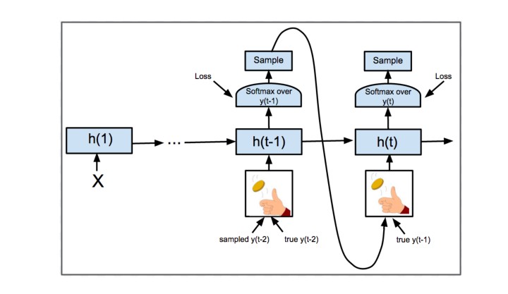
Figure 1: Illustration of the Scheduled Sampling approach, where one flips a coin at every time step to decide to use the true previous token or one sampled from the model itself.

图 1：Scheduled Sampling 方法示意：每个时间步抛一次硬币，决定使用真实的前一个 token，还是使用从模型自己采样得到的 token。

We thus propose to use a schedule to decrease $\epsilon_i$ as a function of $i$ itself, in a similar manner used to decrease the learning rate in most modern stochastic gradient descent approaches. Examples of such schedules can be seen in Figure 2 as follows:

因此我们提议用一个日程，把 $\epsilon_i$ 写成 $i$ 本身的函数并逐渐减小，做法类似于大多数现代随机梯度下降方法里降低学习率。这类日程的例子见图 2，具体如下：

• Linear decay: $\epsilon_i = \max(\epsilon, k - ci)$ where $0 \leq \epsilon < 1$ is the minimum amount of truth to be given to the model and $k$ and $c$ provide the offset and slope of the decay, which depend on the expected speed of convergence.

• 线性衰减：$\epsilon_i = \max(\epsilon, k - ci)$，其中 $0 \leq \epsilon < 1$ 是仍要提供给模型的最少真值比例，$k$ 和 $c$ 给出衰减的偏移和斜率，取决于预期的收敛速度。

• Exponential decay: $\epsilon_i = k^i$ where $k < 1$ is a constant that depends on the expected speed of convergence.

• 指数衰减：$\epsilon_i = k^i$，其中 $k < 1$ 是取决于预期收敛速度的常数。

• Inverse sigmoid decay: $\epsilon_i = k / (k + \exp(i/k))$ where $k \geq 1$ depends on the expected speed of convergence.

• 反 sigmoid 衰减：$\epsilon_i = k / (k + \exp(i/k))$，其中 $k \geq 1$ 取决于预期的收敛速度。

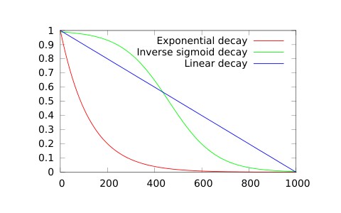
Figure 2: Examples of decay schedules.

图 2：衰减日程的例子。

We call our approach Scheduled Sampling. Note that when we sample the previous token $\hat{y}_{t-1}$ from the model itself while training, we could back-propagate the gradient of the losses at times $t \rightarrow T$ through that decision. This was not done in the experiments described in this paper and is left for future work.

我们把这种方法叫做 Scheduled Sampling。需要注意的是，训练时若从前一个 token $\hat{y}_{t-1}$ 由模型自己采样得到，本可以把时刻 $t \rightarrow T$ 上那些损失的梯度回传到这一决策。本文所述实验没有这样做，留给以后的工作。

3 Related Work

3 相关工作

The discrepancy between the training and inference distributions has already been noticed in the literature, in particular for control and reinforcement learning tasks.

训练分布和推断分布之间的不一致，文献里已经注意到了，尤其是在控制和强化学习任务中。

SEARN [9] was proposed to tackle problems where supervised training examples might be different from actual test examples when each example is made of a sequence of decisions, like acting in a complex environment where a few mistakes of the model early in the sequential decision process might compound and yield a very poor global performance. Their proposed approach involves a meta-algorithm where at each meta-iteration one trains a new model according to the current policy (essentially the expected decisions for each situation), applies it on a test set and modifies the next iteration policy in order to account for the previous decisions and errors. The new policy is thus a combination of the previous one and the actual behavior of the model.

SEARN [9] 针对的是这类问题：每个样本本身是一连串决策，因而有监督的训练样本可能和真正的测试样本不同——例如在复杂环境中行动时，模型在序列决策早期的少量错误就可能累积，导致整体表现非常差。他们提出的方法是一种元算法：每一次元迭代都按当前策略（本质上是每种情形下的期望决策）训练一个新模型，把它用在一个测试集上，再修改下一轮策略，以便把先前的决策和错误考虑进去。于是新策略是上一轮策略与模型实际行为的组合。

In comparison to SEARN and related ideas [10, 11], our proposed approach is completely online: a single model is trained and the policy slowly evolves during training, instead of a batch approach, which makes it much faster to train.[^3] Furthermore, SEARN has been proposed in the context of reinforcement learning, while we consider the supervised learning setting trained using stochastic gradient descent on the overall objective.

与 SEARN 及相关想法 [10, 11] 相比，我们提出的方法是完全在线的：只训练一个模型，策略在训练过程中缓慢演化，而不是一种批量方法，因而训练快得多。[^3] 此外，SEARN 是在强化学习背景下提出的，而我们考虑的是在整体目标上用随机梯度下降训练的监督学习设置。

[^3]: In fact, in the experiments we report in this paper, our proposed approach was not meaningfully slower (nor faster) to train than the baseline.

[^3]：事实上，在本文报告的实验里，我们提出的方法在训练时间上并不比基线明显更慢（也不更快）。

Other approaches have considered the problem from a ranking perspective, in particular for parsing tasks [12] where the target output is a tree. In this case, the authors proposed to use a beam search both during training and inference, so that both phases are aligned. The training beam is used to find the best current estimate of the model, which is compared to the guided solution (the truth) using a ranking loss. Unfortunately, this is not feasible when using a model like a recurrent neural network (which is now the state-of-the-art technique in many sequential tasks), as the state sequence cannot be factored easily (because it is a multi-dimensional continuous state) and thus beam search is hard to use efficiently at training time (as well as inference time, in fact).

另一些方法从排序的角度看待这一问题，尤其是目标输出为树的句法分析任务 [12]。在那种情形里，作者主张在训练和推断时都使用束搜索，好让两个阶段对齐。训练时的束用来找到模型当前的最佳估计，再用排序损失把它和有引导的解（真值）比较。遗憾的是，当使用循环神经网络这类模型（它现在已是许多序列任务上的最先进技术）时，这一做法并不可行，因为状态序列不容易做因式分解（它是多维连续状态），因而束搜索很难在训练时高效使用（事实上在推断时也一样）。

Finally, [13] proposed an online algorithm for parsing problems that adapts the targets through the use of a dynamic oracle that takes into account the decisions of the model. The trained model is a perceptron and is thus not state-based like a recurrent neural network, and the probability of choosing the truth is fixed during training.

最后，[13] 为句法分析问题提出了一种在线算法，通过考虑模型决策的动态 oracle 来调整目标。所训练的模型是感知机，因而并不像循环神经网络那样基于状态，而且选择真值的概率在训练过程中是固定的。

4 Experiments

4 实验

We describe in this section experiments on three different tasks, in order to show that scheduled sampling can be helpful in different settings. We report results on image captioning, constituency parsing and speech recognition.

本节描述三项不同任务上的实验，以表明 scheduled sampling 在不同设置下都能有帮助。我们报告图像描述、成分句法分析和语音识别上的结果。

4.1 Image Captioning

4.1 图像描述

Image captioning has attracted a lot of attention in the past year. The task can be formulated as a mapping of an image onto a sequence of words describing its content in some natural language, and most proposed approaches employ some form of recurrent network structure with simple decoding schemes [5, 6, 14, 15, 16]. A notable exception is the system proposed in [17], which does not directly optimize the log likelihood of the caption given the image, and instead proposes a pipelined approach.

图像描述在过去一年里吸引了很多关注。这项任务可以表述成把一张图像映射成用某种自然语言描述其内容的词序列，大多数方法都采用某种形式的循环网络结构，并配合简单的解码方案 [5, 6, 14, 15, 16]。一个值得注意的例外是 [17] 提出的系统：它并不直接优化给定图像时描述文本的对数似然，而是提出一种流水线方法。

Since an image can have many valid captions, the evaluation of this task is still an open problem. Some attempts have been made to design metrics that positively correlate with human evaluation [18], and a common set of tools have been published by the MSCOCO team [19].

由于一张图像可以有许多同样成立的描述，这项任务的评价仍是一个开放问题。已有一些工作试图设计与人类评价正相关的指标 [18]，MSCOCO 团队也发布了一套常用工具 [19]。

We used the MSCOCO dataset from [19] to train our model. We trained on 75k images and report results on a separate development set of 5k additional images. Each image in the corpus has 5 different captions, so the training procedure picks one at random, creates a mini-batch of examples, and optimizes the objective function defined in (4). The image is preprocessed by a pretrained convolutional neural network (without the last classification layer) similar to the one described in [20], and the resulting image embedding is treated as if it was the first word from which the model starts generating language. The recurrent neural network generating words is an LSTM with one layer of 512 hidden units, and the input words are represented by embedding vectors of size 512. The number of words in the dictionary is 8857. We used an inverse sigmoid decay schedule for $\epsilon_i$ for the scheduled sampling approach.

我们用 [19] 中的 MSCOCO 数据集训练模型：在 7.5 万张图像上训练，并在另外 5 千张图像组成的独立开发集上报告结果。语料中每张图像有 5 条不同描述，因此训练时随机挑一条，组成小批量样本，并优化 (4) 中定义的目标函数。图像先由一个与 [20] 所述类似的、去掉最后分类层的预训练卷积神经网络处理，得到的图像嵌入被当作模型开始生成语言时的“第一个词”。生成词的循环神经网络是一层 512 个隐单元的 LSTM，输入词用 512 维嵌入向量表示。词典大小为 8857。对 scheduled sampling，我们采用反 sigmoid 的 $\epsilon_i$ 衰减日程。

Table 1 shows the results on various metrics on the development set. Each of these metrics is a variant of estimating the overlap between the obtained sequence of words and the target one. Since there were 5 target captions per image, the best result is always chosen. To the best of our knowledge, the baseline results are consistent (slightly better) with the current state-of-the-art on that task. While dropout helped in terms of log likelihood (as expected but not shown), it had a negative impact on the real metrics. On the other hand, scheduled sampling successfully trained a model more resilient to failures due to training and inference mismatch, which likely yielded higher quality captions according to all the metrics. Ensembling models also yielded better performance, both for the baseline and the schedule sampling approach. It is also interesting to note that a model trained while always sampling from itself (hence in a regime similar to inference), dubbed Always Sampling in the table, yielded very poor performance, as expected because the model has a hard time learning the task in that case. We also trained a model with scheduled sampling, but instead of sampling from the model, we sampled from a uniform distribution, in order to verify that it was important to build on the current model and that the performance boost was not just a simple form of regularization. We called this Uniform Scheduled Sampling and the results are better than the baseline, but not as good as our proposed approach. We also experimented with flipping the coin once per sequence instead of once per token, but the results were as poor as the Always Sampling approach.

表 1 给出开发集上各种指标的结果。这些指标都是在估计得到的词序列与目标序列之间重叠程度的变体。由于每张图像有 5 条目标描述，始终取最好的结果。据我们所知，基线结果与该任务当时的最先进水平一致（略好一些）。dropout 在对数似然上有帮助（这一点符合预期，未在表中列出），但对真正的评价指标有负面影响。相比之下，scheduled sampling 成功训练出对训练/推断不一致造成的失败更有韧性的模型，按所有指标看都更可能得到更高质量的描述。对模型做集成也能提高表现，基线和 scheduled sampling 都是如此。同样值得注意的是，若训练时始终从自身采样（因而处于与推断相似的机制），表中称为 Always Sampling，表现会非常差：这是预期中的，因为那时模型很难学会这项任务。我们还训练了一个同样使用 scheduled sampling、但不从模型而从均匀分布采样的模型，以验证“建立在当前模型之上”这一点很重要，性能提升并不仅仅是一种简单的正则。我们称之为 Uniform Scheduled Sampling，其结果好于基线，但不如我们提出的方法。我们也试验过整条序列只抛一次硬币而不是对每个 token 抛一次，结果和 Always Sampling 一样差。

Table 1: Various metrics (the higher the better) on the MSCOCO development set for the image captioning task.

Approach vs Metric	BLEU-4	METEOR	CIDER
Baseline	28.8	24.2	89.5
Baseline with Dropout	28.1	23.9	87.0
Always Sampling	11.2	15.7	49.7
Scheduled Sampling	30.6	24.3	92.1
Uniform Scheduled Sampling	29.2	24.2	90.9
Baseline ensemble of 10	30.7	25.1	95.7
Scheduled Sampling ensemble of 5	32.3	25.4	98.7

表 1：图像描述任务中，MSCOCO 开发集上的各项指标（越高越好）。

方法与指标	BLEU-4	METEOR	CIDER
基线	28.8	24.2	89.5
带 Dropout 的基线	28.1	23.9	87.0
始终采样	11.2	15.7	49.7
Scheduled Sampling	30.6	24.3	92.1
均匀 Scheduled Sampling	29.2	24.2	90.9
10 个基线模型的集成	30.7	25.1	95.7
5 个 Scheduled Sampling 模型的集成	32.3	25.4	98.7

It's worth noting that we used our scheduled sampling approach to participate in the 2015 MSCOCO image captioning challenge [21] and ranked first in the final leaderboard.

值得一提的是，我们用 scheduled sampling 方法参加了 2015 年 MSCOCO 图像描述挑战 [21]，并在最终排行榜上获得第一。

4.2 Constituency Parsing

4.2 成分句法分析

Another less obvious connection with the any-to-sequence paradigm is constituency parsing. Recent work [4] has proposed an interpretation of a parse tree as a sequence of linear “operations” that build up the tree. This linearization procedure allowed them to train a model that can map a sentence onto its parse tree without any modification to the any-to-sequence formulation.

与 any-to-sequence 范式不那么显而易见的另一项联系，是成分句法分析。近期工作 [4] 把句法树解释成一串用来把树搭建起来的线性“操作”。这一线性化手续使他们可以在不对 any-to-sequence 表述做任何修改的情况下，训练一个把句子映射到其句法树的模型。

The trained model has one layer of 512 LSTM cells and words are represented by embedding vectors of size 512. We used an attention mechanism similar to the one described in [22] which helps, when considering the next output token to produce $y_t$, to focus on part of the input sequence only by applying a softmax over the LSTM state vectors corresponding to the input sequence. The input word dictionary contained around 90k words, while the target dictionary contained 128 symbols used to describe the tree. We used an inverse sigmoid decay schedule for $\epsilon_i$ in the scheduled sampling approach.

训练的模型有一层 512 个 LSTM 单元，词用 512 维嵌入向量表示。我们使用了与 [22] 所述类似的注意力机制：在考虑下一个要生成的输出 token $y_t$ 时，对输入序列对应的 LSTM 状态向量做 softmax，从而只把注意力放在输入序列的一部分上。输入词典大约有 9 万词，目标词典则包含 128 个用来描述句法树的符号。对 scheduled sampling，我们采用反 sigmoid 的 $\epsilon_i$ 衰减日程。

Parsing is quite different from image captioning as the function that one has to learn is almost deterministic. In contrast to an image having a large number of valid captions, most sentences have a unique parse tree (although some very difficult cases exist). Thus, the model operates almost deterministically, which can be seen by observing that the train and test perplexities are extremely low compared to image captioning (1.1 vs. 7).

句法分析和图像描述很不一样，因为需要学习的函数几乎是确定性的。与一张图像可以有大量同样成立的描述不同，大多数句子有唯一的句法树（尽管也存在一些非常困难的情形）。因此模型几乎是在确定性机制下运作，从训练和测试困惑度相对图像描述极低（1.1 对 7）也可以看出来。

This different operating regime makes for an interesting comparison, as one would not expect the baseline algorithm to make many mistakes. However, and as can be seen in Table 2, scheduled sampling has a positive effect which is additive to dropout. In this table we report the F1 score on the WSJ 22 development set [23]. We should also emphasize that there are only 40k training instances, so overfitting contributes largely to the performance of our system. Whether the effect of sampling during training helps with regard to overfitting or the training/inference mismatch is unclear, but the result is positive and additive with dropout. Once again, a model trained by always sampling from itself instead of using the groundtruth previous token as input yielded very bad results, in fact so bad that the resulting trees were often not valid trees (hence the “-” in the corresponding F1 metric).

这种不同的运作机制构成了一组有意思的比较，因为按理说基线算法不该犯很多错误。然而，如表 2 所示，scheduled sampling 仍有正面效果，而且与 dropout 是可加的。该表报告的是 WSJ 22 开发集 [23] 上的 F1。还应强调，训练样本只有 4 万条，过拟合对我们系统的表现影响很大。训练时采样的效果究竟是有助于缓解过拟合，还是有助于缓解训练/推断不一致，目前并不清楚，但结果是正面的，并且与 dropout 可加。同样，若训练时始终从自身采样、而不把真实的前一个 token 作为输入，得到的结果非常差，差到生成的树常常根本不是合法树（因此对应的 F1 记为“-”）。

Table 2: F1 score (the higher the better) on the validation set of the parsing task.

Approach	F1
Baseline LSTM	86.54
Baseline LSTM with Dropout	87.0
Always Sampling	–
Scheduled Sampling	88.08
Scheduled Sampling with Dropout	88.68

表 2：句法分析任务验证集上的 F1（越高越好）。

方法	F1
基线 LSTM	86.54
带 Dropout 的基线 LSTM	87.0
始终采样	–
Scheduled Sampling	88.08
带 Dropout 的 Scheduled Sampling	88.68

4.3 Speech Recognition

4.3 语音识别

For the speech recognition experiments, we used a slightly different setting from the rest of the paper. Each training example is an input/output pair $(X, Y)$, where $X$ is a sequence of $T$ input vectors $x_1, x_2, \cdots x_T$ and $Y$ is a sequence of $T$ tokens $y_1, y_2, \cdots y_T$ so each $y_t$ is aligned with the corresponding $x_t$. Here, $x_t$ are the acoustic features represented by log Mel filter bank spectra at frame $t$, and $y_t$ is the corresponding target. The targets used were HMM-state labels generated from a GMM-HMM recipe, using the Kaldi toolkit [24] but could very well have been phoneme labels. This setting is different from the other experiments in that the model we used is the following:

语音识别实验采用的设置与论文其余部分略有不同。每个训练样本是一个输入/输出对 $(X, Y)$，其中 $X$ 是 $T$ 个输入向量的序列 $x_1, x_2, \cdots x_T$，$Y$ 是 $T$ 个 token 的序列 $y_1, y_2, \cdots y_T$，因而每个 $y_t$ 与对应的 $x_t$ 对齐。这里的 $x_t$ 是用第 $t$ 帧的对数 Mel 滤波器组频谱表示的声学特征，$y_t$ 是对应的目标。所用目标是由 GMM-HMM 流程、借助 Kaldi 工具包 [24] 生成的 HMM 状态标签，不过也可以是音素标签。这一设置与其他实验的不同之处在于，我们使用的模型如下：

$$\begin{aligned}
\log P(Y \mid X; \theta) &= \log P(y_1^T \mid x_1^T; \theta) \
&= \sum_{t=1}^{T} \log P(y_t \mid y_1^{t-1}, x_1^t; \theta) \
&= \sum_{t=1}^{T} \log P(y_t \mid h_t; \theta)
\end{aligned} \tag{5}$$

where $h_t$ is computed by a recurrent neural network as follows:

其中 $h_t$ 由循环神经网络按如下方式计算：

$$h_t = \begin{cases}
f(\mathbf{o}h, S, x_1; \theta) & \text{if } t = 1, \
f(h{t-1}, y_{t-1}, x_t; \theta) & \text{otherwise.}
\end{cases} \tag{6}$$

where $\mathbf{o}_h$ is a vector of 0's with same dimensionality as $h_t$'s and $S$ is an extra token added to the dictionary to represent the start of each sequence.

其中 $\mathbf{o}_h$ 是与 $h_t$ 维数相同的全 0 向量，$S$ 是加进词典、用来表示每条序列起点的额外 token。

We generated data for these experiments using the TIMIT[^4] corpus and the KALDI toolkit as described in [25]. Standard configurations were used for the experiments — 40 dimensional log Mel filter banks and their first and second order temporal derivatives were used as inputs to each frame. 180 dimensional targets were generated for each time frame using forced alignment to transcripts using a trained GMM-HMM system. The training, validation and test sets have 3696, 400 and 192 sequences respectively, and their average length was 304 frames. The validation set was used to choose the best epoch in training, and the model parameters from that epoch were used to evaluate the test set.

这些实验的数据用 TIMIT[^4] 语料和 KALDI 工具包按 [25] 所述生成。实验采用标准配置：每一帧的输入是 40 维对数 Mel 滤波器组及其一阶、二阶时间导数；每一时间帧的 180 维目标，则由训练好的 GMM-HMM 系统对转写做强制对齐得到。训练集、验证集和测试集分别有 3696、400 和 192 条序列，平均长度为 304 帧。用验证集选择训练中最好的一轮，再用该轮的模型参数评估测试集。

The trained models had two layers of 250 LSTM cells and a softmax layer, for each of five configurations — a baseline configuration where the ground truth was always fed to the model, a configuration (Always Sampling) where the model was only fed in its own predictions from the last time step, and three scheduled sampling configurations (Scheduled Sampling 1–3), where $\epsilon_i$ was ramped linearly from a maximum value to a minimum value over ten epochs and then kept constant at the final value. For each configuration, we trained 3 models and report average performance over them. Training of each model was done over frame targets from the GMM. The baseline configurations typically reached the best validation accuracy after approximately 14 epochs whereas the sampling models reached the best accuracy after approximately 9 epochs, after which the validation accuracy decreased. This is probably because the way we trained our models is not exact — it does not account for the gradient of the sampling probabilities from which we sampled our targets. Future effort at tackling this problem may further improve results.

所训练的模型都有两层各 250 个 LSTM 单元，外加一层 softmax，共五种配置：始终把真值喂给模型的基线配置；只把模型自己上一时间步的预测喂回去的配置（Always Sampling）；以及三种 scheduled sampling 配置（Scheduled Sampling 1–3），其中 $\epsilon_i$ 在十个周期里从最大值线性降到最小值，之后保持在终值。每种配置我们训练 3 个模型，并报告它们的平均表现。每个模型都在来自 GMM 的帧级目标上训练。基线配置通常大约在 14 个周期后达到最好的验证准确率，而采样模型大约在 9 个周期后达到最好准确率，此后验证准确率下降。这很可能是因为我们训练模型的方式并不精确——它没有考虑我们据以采样目标的那些采样概率的梯度。以后若能处理这个问题，结果或许还能进一步提高。

Testing was done by finding the best sequence from beam search decoding (using a beam size of 10 beams) and computing the error rate over the sequences. We also report the next step error rate (where the model was fed in the ground truth to predict the class of the next frame) for each of the models on the validation set to summarize the performance of the models on the training objective. Table 3 shows a summary of the results.

测试时，用束搜索解码（束宽为 10）找出最佳序列，再计算这些序列上的错误率。我们还在验证集上报告各模型的逐步预测错误率（把真值喂给模型以预测下一帧的类别），用来概括模型在训练目标上的表现。表 3 给出结果摘要。

It can be seen that the baseline performs better next step prediction than the models that sample the tokens for input. This is to be expected, since the former has access to the groundtruth. However, it can be seen that the models that were trained with sampling perform better than the baseline during decoding. It can also be seen that for this problem, the “Always Sampling” model performs quite well. We hypothesize that this has to do with the nature of the dataset. The HMM-aligned states have a lot of correlation — the same state appears as the target for several frames, and most of the states are constrained only to go to a subset of other states. Next step prediction with groundtruth labels on this task ends up paying disproportionate attention to the structure of the labels ($y_1^{t-1}$) and not enough to the acoustics input ($x_1^t$). Thus it achieves very good next step prediction error when the groundtruth sequence is fed in with the acoustic information, but is not able to exploit the acoustic information sufficiently when the groundtruth sequence is not fed in. For this model the testing conditions are too far from the training condition for it to make good predictions. The model that is only fed its own prediction (Always Sampling) ends up exploiting all the information it can find in the acoustic signal, and effectively ignores its own predictions to influence the next step prediction. Thus at test time, it performs just as well as it does during training. A model such as the attention model of [26] which predicts phone sequences directly, instead of the highly redundant HMM state sequences, would not suffer from this problem because it would need to exploit both the acoustic signal and the language model sufficiently to make predictions. Nevertheless, even in this setting, adding scheduled sampling still helped to improve the decoding frame error rate.

可以看到，基线的逐步预测好于那些对输入 token 做采样的模型。这是预期之中的，因为前者能拿到真值。然而也可以看到，用采样训练的模型在解码时好于基线。还可以看到，对这个问题，“Always Sampling”模型表现相当好。我们猜想这与数据集的性质有关。HMM 对齐的状态有很强的相关性：同一个状态会作为连续若干帧的目标出现，而且大多数状态只被约束转移到其他状态的一个子集。在这个任务上，用真值标签做逐步预测，最终会把过多注意力放在标签结构（$y_1^{t-1}$）上，而对声学输入（$x_1^t$）关注不够。于是，当把真值序列连同声学信息一起喂进去时，逐步预测误差会非常好；但一旦不喂真值序列，它就不能充分挖掘声学信息。对这种模型来说，测试条件离训练条件太远，因而难以做出好的预测。只被喂给自己预测的模型（Always Sampling）则会尽可能利用声学信号里能找到的全部信息，并实际上忽略自己的预测对下一步预测的影响。因此在测试时，它的表现和训练时一样好。若采用 [26] 那样的注意力模型，直接预测音素序列而不是高度冗余的 HMM 状态序列，就不会有这个问题，因为它必须同时充分利用声学信号和语言模型才能做预测。尽管如此，即使在这一设置下，加入 scheduled sampling 仍然有助于降低解码帧错误率。

Note that typically speech recognition experiments use HMMs to decode predictions from neural networks in a hybrid model. Here we avoid using an HMM altogether and hence we do not have the advantage of the smoothing that results from the HMM architecture and the language models. Thus the results are not directly comparable to the typical hybrid model results.

需要说明，语音识别实验通常会在混合模型里用 HMM 来解码神经网络的预测。这里我们完全不用 HMM，因而也没有 HMM 架构和语言模型所带来的平滑好处。因此这些结果不能直接与典型的混合模型结果相比。

Table 3: Frame Error Rate (FER) on the speech recognition experiments. In next step prediction (reported on validation set) the ground truth is fed in to predict the next target like it is done during training. In decoding experiments (reported on test set), beam searching is done to find the best sequence. We report results on four different linear schedulings of sampling, where $\epsilon_i$ was ramped down linearly from $\epsilon_s$ to $\epsilon_e$. For the baseline, the model was only fed in the ground truth. See Section 4.3 for an analysis of the results.

Approach	$\epsilon_s$	$\epsilon_e$	Next Step FER	Decoding FER
Always Sampling	0	0	34.6	35.8
Scheduled Sampling 1	0.25	0	34.3	34.5
Scheduled Sampling 2	0.5	0	34.1	35.0
Scheduled Sampling 3	0.9	0.5	19.8	42.0
Baseline LSTM	1	1	15.0	46.0

表 3：语音识别实验中的帧错误率（FER）。在逐步预测（于验证集上报告）中，像训练时一样把真值喂进去以预测下一个目标。在解码实验（于测试集上报告）中，用束搜索寻找最佳序列。我们报告四种不同线性采样日程的结果，其中 $\epsilon_i$ 从 $\epsilon_s$ 线性降到 $\epsilon_e$。对基线而言，模型只被喂给真值。结果分析见第 4.3 节。

方法	$\epsilon_s$	$\epsilon_e$	逐步预测 FER	解码 FER
始终采样	0	0	34.6	35.8
Scheduled Sampling 1	0.25	0	34.3	34.5
Scheduled Sampling 2	0.5	0	34.1	35.0
Scheduled Sampling 3	0.9	0.5	19.8	42.0
基线 LSTM	1	1	15.0	46.0

5 Conclusion

5 结论

Using recurrent neural networks to predict sequences of tokens has many useful applications like machine translation and image description. However, the current approach to training them, predicting one token at a time, conditioned on the state and the previous correct token, is different from how we actually use them and thus is prone to the accumulation of errors along the decision paths. In this paper, we proposed a curriculum learning approach to slowly change the training objective from an easy task, where the previous token is known, to a realistic one, where it is provided by the model itself. Experiments on several sequence prediction tasks yield performance improvements, while not incurring longer training times. Future work includes back-propagating the errors through the sampling decisions, as well as exploring better sampling strategies including conditioning on some confidence measure from the model itself.

用循环神经网络预测 token 序列，有机器翻译和图像描述等许多有用的应用。然而目前的训练做法是一次预测一个 token，并以状态和前一个正确 token 为条件，这与我们实际使用它们的方式不同，因而容易沿决策路径累积误差。本文提出一种课程学习方法，把训练目标从“前一个 token 已知”的容易任务，慢慢改成“前一个 token 由模型自己提供”的现实任务。若干序列预测任务上的实验带来了性能提升，同时并没有让训练时间变长。未来的工作包括把误差回传到采样决策，以及探索更好的采样策略，包括以模型自身的某种置信度度量为条件。

References

[1] Y. Bengio, P. Simard, and P. Frasconi. Learning long term dependencies is hard. IEEE Transactions on Neural Networks, 5(2):157–166, 1994.

[2] S. Hochreiter and J. Schmidhuber. Long short-term memory. Neural Computation, 9(8), 1997.

[3] I. Sutskever, O. Vinyals, and Q. Le. Sequence to sequence learning with neural networks. In Advances in Neural Information Processing Systems, NIPS, 2014.

[4] O. Vinyals, L. Kaiser, T. Koo, S. Petrov, I. Sutskever, and G. Hinton. Grammar as a foreign language. In arXiv:1412.7449, 2014.

[5] O. Vinyals, A. Toshev, S. Bengio, and D. Erhan. Show and tell: A neural image caption generator. In IEEE Conference on Computer Vision and Pattern Recognition, CVPR, 2015.

[6] J. Donahue, L. A. Hendricks, S. Guadarrama, M. Rohrbach, S. Venugopalan, K. Saenko, and T. Darrell. Long-term recurrent convolutional networks for visual recognition and description. In IEEE Conference on Computer Vision and Pattern Recognition, CVPR, 2015.

[7] Y. Bengio, J. Louradour, R. Collobert, and J. Weston. Curriculum learning. In Proceedings of the International Conference on Machine Learning, ICML, 2009.

[8] J. D. Lafferty, A. McCallum, and F. C. N. Pereira. Conditional random fields: Probabilistic models for segmenting and labeling sequence data. In Proceedings of the Eighteenth International Conference on Machine Learning, ICML, pages 282–289, San Francisco, CA, USA, 2001. Morgan Kaufmann Publishers Inc.

[9] H. Daumé III, J. Langford, and D. Marcu. Search-based structured prediction as classification. Machine Learning Journal, 2009.

[10] S. Ross, G. J. Gordon, and J. A. Bagnell. A reduction of imitation learning and structured prediction to no-regret online learning. In Proceedings of the Workshop on Artificial Intelligence and Statistics, AISTATS, 2011.

[11] A. Venkatraman, M. Herbert, and J. A. Bagnell. Improving multi-step prediction of learned time series models. In Twenty-Ninth AAAI Conference on Artificial Intelligence, AAAI, 2015.

[12] M. Collins and B. Roark. Incremental parsing with the perceptron algorithm. In Proceedings of the Association for Computational Linguistics, ACL, 2004.

[13] Y. Goldberg and J. Nivre. A dynamic oracle for arc-eager dependency parsing. In Proceedings of COLING, 2012.

[14] J. Mao, W. Xu, Y. Yang, J. Wang, Z. H. Huang, and A. Yuille. Deep captioning with multimodal recurrent neural networks (m-rnn). In International Conference on Learning Representations, ICLR, 2015.

[15] R. Kiros, R. Salakhutdinov, and R. Zemel. Unifying visual-semantic embeddings with multimodal neural language models. In TACL, 2015.

[16] A. Karpathy and F.-F. Li. Deep visual-semantic alignments for generating image descriptions. In IEEE Conference on Computer Vision and Pattern Recognition, CVPR, 2015.

[17] H. Fang, S. Gupta, F. Iandola, R. K. Srivastava, L. Deng, P. Dollar, J. Gao, X. He, M. Mitchell, J. C. Platt, C. L. Zitnick, and G. Zweig. From captions to visual concepts and back. In IEEE Conference on Computer Vision and Pattern Recognition, CVPR, 2015.

[18] R. Vedantam, C. L. Zitnick, and D. Parikh. CIDEr: Consensus-based image description evaluation. In IEEE Conference on Computer Vision and Pattern Recognition, CVPR, 2015.

[19] T.-Y. Lin, M. Maire, S. Belongie, J. Hays, P. Perona, D. Ramanan, P. Dollár, and C. L. Zitnick. Microsoft coco: Common objects in context. arXiv:1405.0312, 2014.

[20] S. Ioffe and C. Szegedy. Batch normalization: Accelerating deep network training by reducing internal covariate shift. In Proceedings of the International Conference on Machine Learning, ICML, 2015.

[21] Y. Cui, M. R. Ronchi, T.-Y. Lin, P. Dollr, and L. Zitnick. Microsoft coco captioning challenge. http://mscoco.org/dataset/#captions-challenge2015, 2015.

[22] D. Bahdanau, K. Cho, and Y. Bengio. Neural machine translation by jointly learning to align and translate. In International Conference on Learning Representations, ICLR, 2015.

[23] E. Hovy, M. Marcus, M. Palmer, L. Ramshaw, and R. Weischedel. Ontonotes: The 90% solution. In Proceedings of the Human Language Technology Conference of the NAACL, Short Papers, pages 57–60, New York City, USA, June 2006. Association for Computational Linguistics.

[24] D. Povey, A. Ghoshal, G. Boulianne, L. Burget, O. Glembek, N. Goel, M. Hannemann, P. Motlicek, Y. Qian, P. Schwarz, J. Silovsky, G. Stemmer, and K. Vesely. The kaldi speech recognition toolkit. In IEEE 2011 Workshop on Automatic Speech Recognition and Understanding. IEEE Signal Processing Society, December 2011. IEEE Catalog No.: CFP11SRW-USB.

[25] N. Jaitly. Exploring Deep Learning Methods for discovering features in speech signals. PhD thesis, University of Toronto, 2014.

[26] Jan Chorowski, Dzmitry Bahdanau, Kyunghyun Cho, and Yoshua Bengio. End-to-end continuous speech recognition using attention-based recurrent nn: First results. arXiv preprint arXiv:1412.1602, 2014.