Scaling Rectified Flow Transformers for High-Resolution Image Synthesis
Scaling Rectified Flow Transformers for High-Resolution Image Synthesis
面向高分辨率图像合成的缩放整流流 Transformer
Patrick Esser Sumith Kulal Andreas Blattmann Rahim Entezari Jonas Müller Harry Saini Yam Levi Dominik Lorenz Axel Sauer Frederic Boesel Dustin Podell Tim Dockhorn Zion English Kyle Lacey Alex Goodwin Yannik Marek Robin Rombach Correspondence to: <first.last>@stability.ai
Abstract
摘要
Diffusion models create data from noise by inverting the forward paths of data towards noise and have emerged as a powerful generative modeling technique for high-dimensional, perceptual data such as images and videos. Rectified flow is a recent generative model formulation that connects data and noise in a straight line. Despite its better theoretical properties and conceptual simplicity, it is not yet decisively established as standard practice. In this work, we improve existing noise sampling techniques for training rectified flow models by biasing them towards perceptually relevant scales. Through a large-scale study, we demonstrate the superior performance of this approach compared to established diffusion formulations for high-resolution text-to-image synthesis. Additionally, we present a novel transformer-based architecture for text-to-image generation that uses separate weights for the two modalities and enables a bidirectional flow of information between image and text tokens, improving text comprehension, typography, and human preference ratings. We demonstrate that this architecture follows predictable scaling trends and correlates lower validation loss to improved text-to-image synthesis as measured by various metrics and human evaluations. Our largest models outperform state-of-the-art models, and we will make our experimental data, code, and model weights publicly available.
扩散模型通过反转数据走向噪声的前向路径,从噪声生成数据,已成为图像与视频等高维感知数据上强有力的生成建模技术。整流流(rectified flow)是近期提出的生成模型形式,把数据与噪声连成直线。尽管理论性质更好、概念更简洁,它尚未成为标准实践。本文改进整流流训练中的噪声采样,使其更偏向感知相关尺度;大规模研究表明,相对既有扩散公式,该做法在高分辨率文生图上表现更优。此外,我们提出一种面向文生图的新型 Transformer 架构:两模态使用独立权重,并在图像与文本 token 之间做双向信息流,从而提升文本理解、排版与人类偏好评分。我们证明该架构遵循可预测的缩放趋势,验证损失降低与按多种指标及人类评估衡量的文生图改进相关。我们最大的模型超过现有最优;实验数据、代码与模型权重将公开。
Keywords:
Stability AI
关键词:
Stability AI
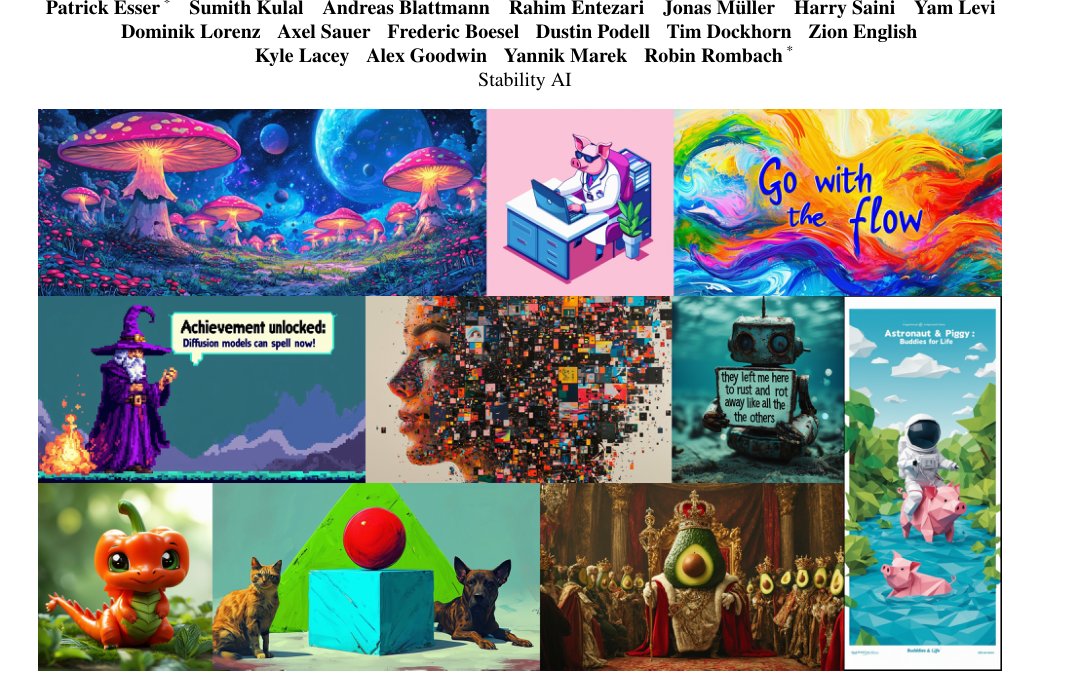
Figure 1: High-resolution samples from our 8B rectified flow model, showcasing its capabilities in typography, precise prompt following and spatial reasoning, attention to fine details, and high image quality across a wide variety of styles.
图 1:我们 8B 整流流模型的高分辨率样本,展示其在排版、精确遵循提示与空间推理、关注细节以及跨多样风格的高图像质量等方面的能力。
1 Introduction
1 引言
Diffusion models create data from noise (Song et al., 2020). They are trained to invert forward paths of data towards random noise and, thus, in conjunction with approximation and generalization properties of neural networks, can be used to generate new data points that are not present in the training data but follow the distribution of the training data (Sohl-Dickstein et al., 2015; Song & Ermon, 2020). This generative modeling technique has proven to be very effective for modeling high-dimensional, perceptual data such as images (Ho et al., 2020). In recent years, diffusion models have become the de-facto approach for generating high-resolution images and videos from natural language inputs with impressive generalization capabilities (Saharia et al., 2022b; Ramesh et al., 2022; Rombach et al., 2022; Podell et al., 2023; Dai et al., 2023; Esser et al., 2023; Blattmann et al., 2023b; Betker et al., 2023; Blattmann et al., 2023a; Singer et al., 2022). Due to their iterative nature and the associated computational costs, as well as the long sampling times during inference, research on formulations for more efficient training and/or faster sampling of these models has increased (Karras et al., 2023; Liu et al., 2022).
扩散模型从噪声生成数据 (Song et al., 2020)。它们被训练以反转数据走向随机噪声的前向路径,因而结合神经网络的逼近与泛化性质,可用于生成训练数据中不存在、但遵循训练数据分布的新数据点 (Sohl-Dickstein et al., 2015; Song & Ermon, 2020)。这一生成建模技术对图像等高维感知数据尤为有效 (Ho et al., 2020)。近年来,扩散模型已成为从自然语言生成高分辨率图像与视频的默认路径,并展现出可观的泛化能力 (Saharia et al., 2022b; Ramesh et al., 2022; Rombach et al., 2022; Podell et al., 2023; Dai et al., 2023; Esser et al., 2023; Blattmann et al., 2023b; Betker et al., 2023; Blattmann et al., 2023a; Singer et al., 2022)。由于其迭代特性与相关计算开销,以及推理时采样时间较长,围绕更高效训练与/或更快采样的公式研究也在增多 (Karras et al., 2023; Liu et al., 2022)。
While specifying a forward path from data to noise leads to efficient training, it also raises the question of which path to choose. This choice can have important implications for sampling. For example, a forward process that fails to remove all noise from the data can lead to a discrepancy in training and test distribution and result in artifacts such as gray image samples (Lin et al., 2024). Importantly, the choice of the forward process also influences the learned backward process and, thus, the sampling efficiency. While curved paths require many integration steps to simulate the process, a straight path could be simulated with a single step and is less prone to error accumulation. Since each step corresponds to an evaluation of the neural network, this has a direct impact on the sampling speed.
指定从数据到噪声的前向路径虽使训练高效,却引出「选哪条路径」的问题。这一选择对采样有重要影响。例如,若前向过程未能从数据中去掉全部噪声,就会造成训练与测试分布不一致,并出现灰色图像样本等伪影 (Lin et al., 2024)。更关键的是,前向过程的选择也会影响学到的反向过程,进而影响采样效率。弯曲路径需要许多积分步才能模拟,而直线路径原则上只需一步,且更不易累积误差。每一步对应一次神经网络求值,因而直接关系到采样速度。
A particular choice for the forward path is a so-called Rectified Flow (Liu et al., 2022; Albergo & Vanden-Eijnden, 2022; Lipman et al., 2023), which connects data and noise on a straight line. Although this model class has better theoretical properties, it has not yet become decisively established in practice. So far, some advantages have been empirically demonstrated in small and medium-sized experiments (Ma et al., 2024), but these are mostly limited to class-conditional models. In this work, we change this by introducing a re-weighting of the noise scales in rectified flow models, similar to noise-predictive diffusion models (Ho et al., 2020). Through a large-scale study, we compare our new formulation to existing diffusion formulations and demonstrate its benefits.
前向路径的一种特定选择是所谓的整流流(Rectified Flow) (Liu et al., 2022; Albergo & Vanden-Eijnden, 2022; Lipman et al., 2023),它把数据与噪声连成直线。尽管该类模型理论性质更好,实践中却尚未被广泛确立。迄今在中小规模实验中已实证出若干优势 (Ma et al., 2024),但多限于类别条件模型。本文改变这一点:我们对照噪声预测扩散模型 (Ho et al., 2020),为整流流引入噪声尺度的重加权。通过大规模研究,我们把新公式与既有扩散公式对比,并展示其收益。
We show that the widely used approach for text-to-image synthesis, where a fixed text representation is fed directly into the model (e.g., via cross-attention (Vaswani et al., 2017; Rombach et al., 2022)), is not ideal, and present a new architecture that incorporates learnable streams for both image and text tokens, which enables a two-way flow of information between them. We combine this with our improved rectified flow formulation and investigate its scalability. We demonstrate a predictable scaling trend in the validation loss and show that a lower validation loss correlates strongly with improved automatic and human evaluations.
我们表明:当前文生图的主流做法——把固定文本表示直接送入模型(例如经交叉注意力 (Vaswani et al., 2017; Rombach et al., 2022))——并不理想;并提出一种新架构,为图像与文本 token 各设可学习流,使二者双向交换信息。我们把它与改进后的整流流公式结合并考察可扩展性。我们在验证损失上观察到可预测的缩放趋势,并表明更低的验证损失与自动指标及人类评估的改进强相关。
Our largest models outperform state-of-the art open models such as SDXL (Podell et al., 2023), SDXL-Turbo (Sauer et al., 2023), Pixart- (Chen et al., 2023), and closed-source models such as DALL-E 3 (Betker et al., 2023) both in quantitative evaluation (Ghosh et al., 2023) of prompt understanding and human preference ratings.
我们最大的模型在提示理解的定量评估 (Ghosh et al., 2023) 与人类偏好评分上,均超过开源最优如 SDXL (Podell et al., 2023)、SDXL-Turbo (Sauer et al., 2023)、Pixart- (Chen et al., 2023),以及闭源如 DALL-E 3 (Betker et al., 2023)。
The core contributions of our work are: (i) We conduct a large-scale, systematic study on different diffusion model and rectified flow formulations to identify the best setting. For this purpose, we introduce new noise samplers for rectified flow models that improve performance over previously known samplers. (ii) We devise a novel, scalable architecture for text-to-image synthesis that allows bi-directional mixing between text and image token streams within the network. We show its benefits compared to established backbones such as UViT (Hoogeboom et al., 2023) and DiT (Peebles & Xie, 2023). Finally, we (iii) perform a scaling study of our model and demonstrate that it follows predictable scaling trends. We show that a lower validation loss correlates strongly with improved text-to-image performance assessed via metrics such as T2I-CompBench (Huang et al., 2023), GenEval (Ghosh et al., 2023) and human ratings. We make results, code, and model weights publicly available.
本文核心贡献如下:(i) 我们对多种扩散与整流流公式做大规模系统研究,以确定最佳设定;为此引入新的整流流噪声采样器,相对既有采样器提升表现。(ii) 我们设计一种可扩展的文生图架构,在网络内部允许文本与图像 token 流双向混合;相对 UViT (Hoogeboom et al., 2023) 与 DiT (Peebles & Xie, 2023) 等既有骨干,我们展示其优势。最后,(iii) 我们对模型做缩放研究,表明其遵循可预测的缩放趋势;验证损失降低与经 T2I-CompBench (Huang et al., 2023)、GenEval (Ghosh et al., 2023) 及人类评分衡量的文生图表现强相关。结果、代码与模型权重将公开。
2 Simulation-Free Training of Flows
2 无需仿真的流训练
We consider generative models that define a mapping between samples from a noise distribution to samples from a data distribution in terms of an ordinary differential equation (ODE),
我们考虑这样一类生成模型:用常微分方程(ODE)定义从噪声分布 的样本 到数据分布 的样本 的映射,
where the velocity is parameterized by the weights of a neural network. Prior work by Chen et al. (2018) suggested to directly solve Equation 1 via differentiable ODE solvers. However, this process is computationally expensive, especially for large network architectures that parameterize . A more efficient alternative is to directly regress a vector field that generates a probability path between and . To construct such a , we define a forward process, corresponding to a probability path between and , as
其中速度 由神经网络权重 参数化。Chen et al. (2018) 曾建议用可微 ODE 求解器直接求解式 1,但对参数化 的大型网络而言计算昂贵。更高效的做法是直接回归一个在 与 之间生成概率路径的向量场 。为构造这样的 ,我们定义前向过程,对应 与 之间的概率路径 :
For and , the marginals,
当 且 时,边缘分布
are consistent with the data and noise distribution.
与数据及噪声分布一致。
To express the relationship between and , we introduce and as
为表达 、 与 的关系,我们引入 与 如下
Since can be written as solution to the ODE , with initial value , generates . Remarkably, one can construct a marginal vector field which generates the marginal probability paths (Lipman et al., 2023) (see B.1), using the conditional vector fields :
由于 可写成 ODE 、初值 的解, 生成 。值得注意的是,可用条件向量场 构造生成边缘概率路径 的边缘向量场 (Lipman et al., 2023)(见 B.1):
While regressing with the Flow Matching objective
若用流匹配目标直接回归
directly is intractable due to the marginalization in Equation 6, Conditional Flow Matching (see B.1),
因式 6 中的边缘化而不可行;条件流匹配(见 B.1)
with the conditional vector fields provides an equivalent yet tractable objective.
借助条件向量场 ,给出等价且可计算的目标。
To convert the loss into an explicit form we insert and into (5)
为把损失写成显式形式,将 与 代入 (5)
Now, consider the signal-to-noise ratio . With , we can rewrite Equation 9 as
现考虑信噪比 。由 ,可把式 9 改写为
Next, we use Equation 10 to reparameterize Equation 8 as a noise-prediction objective:
接着用式 10 把式 8 重参数化为噪声预测目标:
where we defined .
其中定义 。
Note that the optimum of the above objective does not change when introducing a time-dependent weighting. Thus, one can derive various weighted loss functions that provide a signal towards the desired solution but might affect the optimization trajectory. For a unified analysis of different approaches, including classic diffusion formulations, we can write the objective in the following form (following Kingma & Gao (2023)):
注意:引入依赖时间的权重并不改变上述目标的最优解。因此可导出多种加权损失,它们都指向同一期望解,但可能影响优化轨迹。为统一分析包括经典扩散在内的不同做法,我们把目标写成如下形式(依 Kingma & Gao (2023)):
where corresponds to .
其中 对应 。
3 Flow Trajectories
3 流轨迹
In this work, we consider different variants of the above formalism that we briefly describe in the following.
本文考虑上述形式体系的若干变体,简述如下。
Rectified Flow
Rectified Flows (RFs) (Liu et al., 2022; Albergo & Vanden-Eijnden, 2022; Lipman et al., 2023) define the forward process as straight paths between the data distribution and a standard normal distribution, i.e.
整流流
整流流(RF)(Liu et al., 2022; Albergo & Vanden-Eijnden, 2022; Lipman et al., 2023) 把前向过程定义为数据分布与标准正态之间的直线路径,即
and uses which then corresponds to . The network output directly parameterizes the velocity .
并使用 ,此时对应 。网络输出直接参数化速度 。
EDM
EDM (Karras et al., 2022) uses a forward process of the form
EDM
EDM (Karras et al., 2022) 使用如下形式的前向过程
where (Kingma & Gao, 2023) with being the quantile function of the normal distribution with mean and variance . Note that this choice results in
其中 (Kingma & Gao, 2023) , 为均值 、方差 的正态分位数函数。该选择导致
The network is parameterized through an F-prediction (Kingma & Gao, 2023; Karras et al., 2022) and the loss can be written as with
网络经 F-预测参数化 (Kingma & Gao, 2023; Karras et al., 2022),损失可写成 ,其中
Cosine
(Nichol & Dhariwal, 2021) proposed a forward process of the form
余弦
(Nichol & Dhariwal, 2021) 提出如下形式的前向过程
In combination with an -parameterization and loss, this corresponds to a weighting . When combined with a v-prediction loss (Kingma & Gao, 2023), the weighting is given by .
与 -参数化及损失结合时,对应权重 。与 v-预测损失结合时 (Kingma & Gao, 2023),权重为 。
(LDM-)Linear
LDM (Rombach et al., 2022) uses a modification of the DDPM schedule (Ho et al., 2020). Both are variance preserving schedules, i.e. , and define for discrete timesteps in terms of diffusion coefficients as . For given boundary values and , DDPM uses and LDM uses .
(LDM-)线性
LDM (Rombach et al., 2022) 使用 DDPM 日程 (Ho et al., 2020) 的变体。二者皆为方差保持日程,即 ,并对离散时间步 用扩散系数 定义 。给定边界 与 ,DDPM 取 ,LDM 取 。
3.1 Tailored SNR Samplers for RF models
3.1 面向 RF 模型的定制 SNR 采样器
The RF loss trains the velocity uniformly on all timesteps in . Intuitively, however, the resulting velocity prediction target is more difficult for in the middle of , since for , the optimal prediction is the mean of , and for the optimal prediction is the mean of . In general, changing the distribution over from the commonly used uniform distribution to a distribution with density is equivalent to a weighted loss with
RF 损失在 上均匀训练速度 。直观上,所得速度预测目标 在区间中部更难:在 时最优预测是 的均值,在 时是 的均值。一般而言,把 上常用的均匀分布 换成密度为 的分布,等价于加权损失 ,其中
Thus, we aim to give more weight to intermediate timesteps by sampling them more frequently. Next, we describe the timestep densities that we use to train our models.
因此我们希望更频繁地采样中间时间步,以给予更大权重。下面描述用于训练的时间步密度 。
Logit-Normal Sampling
One option for a distribution that puts more weight on intermediate steps is the logit-normal distribution (Atchison & Shen, 1980). Its density,
Logit-正态采样
一种给中间步更大权重的分布是 logit-正态分布 (Atchison & Shen, 1980)。其密度
where , has a location parameter, , and a scale parameter, . The location parameter enables us to bias the training timesteps towards either data (negative ) or noise (positive ). As shown in Figure 11, the scale parameters controls how wide the distribution is.
其中 ,具有位置参数 与尺度参数 。位置参数可将训练时间步偏向数据 (负 )或噪声 (正 )。如图 11 所示,尺度参数控制分布宽度。
In practice, we sample the random variable from a normal distribution and map it through the standard logistic function.
实践中,我们从正态 采样,再经标准 logistic 函数映射。
Mode Sampling with Heavy Tails
The logit-normal density always vanishes at the endpoints and . To study whether this has adverse effects on the performance, we also use a timestep sampling distribution with strictly positive density on . For a scale parameter , we define
带重尾的众数采样
logit-正态密度在端点 与 处总为零。为考察这是否损害表现,我们也使用在 上严格正密度的时间步采样分布。对尺度参数 ,定义
For , this function is monotonic, and we can use it to sample from the implied density . As seen in Figure 11, the scale parameter controls the degree to which either the midpoint (positive ) or the endpoints (negative ) are favored during sampling. This formulation also includes a uniform weighting for , which has been used widely in previous works on Rectified Flows (Liu et al., 2022; Ma et al., 2024).
对 ,该函数单调,可用其从隐含密度 采样。如图 11,尺度参数控制采样时更偏向中点(正 )还是端点(负 )。该形式在 时包含均匀加权 ,此前整流流工作中广泛使用 (Liu et al., 2022; Ma et al., 2024)。
CosMap
Finally, we also consider the cosine schedule (Nichol & Dhariwal, 2021) from Section 3 in the RF setting. In particular, we are looking for a mapping , such that the log-snr matches that of the cosine schedule: . Solving for , we obtain for
CosMap
最后,我们也在 RF 设定下考虑第 3 节的余弦日程 (Nichol & Dhariwal, 2021)。具体地,我们寻找映射 ,使 log-snr 与余弦日程匹配:。求解 ,对 得到
from which we obtain the density
由此得到密度
4 Text-to-Image Architecture
4 文生图架构
(a) Overview of all components.
(a) 全部组件总览。
For text-conditional sampling of images, our model has to take both modalities, text and images, into account. We use pretrained models to derive suitable representations and then describe the architecture of our diffusion backbone. An overview of this is presented in Figure 2.
为做文本条件的图像采样,模型须同时考虑文本与图像两种模态。我们用预训练模型得到合适表示,再描述扩散骨干架构。总览见图 2。
Our general setup follows LDM (Rombach et al., 2022) for training text-to-image models in the latent space of a pretrained autoencoder. Similar to the encoding of images to latent representations, we also follow previous approaches (Saharia et al., 2022b; Balaji et al., 2022) and encode the text conditioning using pretrained, frozen text models. Details can be found in Section B.2.
总体设定遵循 LDM (Rombach et al., 2022),在预训练自编码器的潜空间中训练文生图模型。与把图像编成潜表示类似,我们也沿用既有做法 (Saharia et al., 2022b; Balaji et al., 2022),用预训练、冻结的文本模型编码文本条件 。细节见第 B.2 节。
Multimodal Diffusion Backbone Our architecture builds upon the DiT (Peebles & Xie, 2023) architecture. DiT only considers class conditional image generation and uses a modulation mechanism to condition the network on both the timestep of the diffusion process and the class label. Similarly, we use embeddings of the timestep and as inputs to the modulation mechanism. However, as the pooled text representation retains only coarse-grained information about the text input (Podell et al., 2023), the network also requires information from the sequence representation .
多模态扩散骨干 我们的架构建立在 DiT (Peebles & Xie, 2023) 之上。DiT 只考虑类别条件图像生成,并用调制机制把网络条件到扩散时间步与类别标签。类似地,我们用时间步 与 的嵌入作为调制输入。但由于池化后的文本表示只保留粗粒度信息 (Podell et al., 2023),网络还需要序列表示 中的信息。
We construct a sequence consisting of embeddings of the text and image inputs. Specifically, we add positional encodings and flatten patches of the latent pixel representation to a patch encoding sequence of length . After embedding this patch encoding and the text encoding to a common dimensionality, we concatenate the two sequences. We then follow DiT and apply a sequence of modulated attention and MLPs.
我们构造由文本与图像嵌入组成的序列。具体地,为潜像素表示 的 patch 加入位置编码并展平,得到长度为 的 patch 编码序列。将该 patch 编码与文本编码 嵌入到共同维度后拼接。随后按 DiT,施加一系列经调制的注意力与 MLP。
Since text and image embeddings are conceptually quite different, we use two separate sets of weights for the two modalities. As shown in Figure 2(b), this is equivalent to having two independent transformers for each modality, but joining the sequences of the two modalities for the attention operation, such that both representations can work in their own space yet take the other one into account.
由于文本与图像嵌入在概念上差异较大,我们为两模态使用两套独立权重。如图 2(b) 所示,这等价于每模态各有一个独立 Transformer,但在注意力运算时把两模态序列拼在一起,使二者各自在自己的空间工作,又能互相参照。
For our scaling experiments, we parameterize the size of the model in terms of the model’s depth , i.e. the number of attention blocks, by setting the hidden size to (expanded to channels in the MLP blocks), and the number of attention heads equal to .
在缩放实验中,我们用模型深度 (即注意力块数)参数化规模:隐层大小取 (MLP 块中扩展到 通道),注意力头数等于 。
5 Experiments
5 实验
| rank averaged over | |||
|---|---|---|---|
| variant | all | 5 steps | 50 steps |
| rf/lognorm(0.00, 1.00) | 01.54 | 01.25 | 01.50 |
| rf/lognorm(1.00, 0.60) | 02.08 | 03.50 | 02.00 |
| rf/lognorm(0.50, 0.60) | 02.71 | 08.50 | 01.00 |
| rf/mode(1.29) | 02.75 | 03.25 | 03.00 |
| rf/lognorm(0.50, 1.00) | 02.83 | 01.50 | 02.50 |
| eps/linear | 02.88 | 04.25 | 02.75 |
| rf/mode(1.75) | 03.33 | 02.75 | 02.75 |
| rf/cosmap | 04.13 | 03.75 | 04.00 |
| edm(0.00, 0.60) | 05.63 | 13.25 | 03.25 |
| rf | 05.67 | 06.50 | 05.75 |
| v/linear | 06.83 | 05.75 | 07.75 |
| edm(0.60, 1.20) | 09.00 | 13.00 | 09.00 |
| v/cos | 09.17 | 12.25 | 08.75 |
| edm/cos | 11.04 | 14.25 | 11.25 |
| edm/rf | 13.04 | 15.25 | 13.25 |
| edm(-1.20, 1.20) | 15.58 | 20.25 | 15.00 |
Table 1: Global ranking of variants. For this ranking, we apply non-dominated sorting averaged over EMA and non-EMA weights, two datasets and different sampling settings.
| 平均排序 | |||
|---|---|---|---|
| 变体 | 全部 | 5 步 | 50 步 |
| rf/lognorm(0.00, 1.00) | 01.54 | 01.25 | 01.50 |
| rf/lognorm(1.00, 0.60) | 02.08 | 03.50 | 02.00 |
| rf/lognorm(0.50, 0.60) | 02.71 | 08.50 | 01.00 |
| rf/mode(1.29) | 02.75 | 03.25 | 03.00 |
| rf/lognorm(0.50, 1.00) | 02.83 | 01.50 | 02.50 |
| eps/linear | 02.88 | 04.25 | 02.75 |
| rf/mode(1.75) | 03.33 | 02.75 | 02.75 |
| rf/cosmap | 04.13 | 03.75 | 04.00 |
| edm(0.00, 0.60) | 05.63 | 13.25 | 03.25 |
| rf | 05.67 | 06.50 | 05.75 |
| v/linear | 06.83 | 05.75 | 07.75 |
| edm(0.60, 1.20) | 09.00 | 13.00 | 09.00 |
| v/cos | 09.17 | 12.25 | 08.75 |
| edm/cos | 11.04 | 14.25 | 11.25 |
| edm/rf | 13.04 | 15.25 | 13.25 |
| edm(-1.20, 1.20) | 15.58 | 20.25 | 15.00 |
表 1:各变体的全局排序。 该排序对 EMA 与非 EMA 权重、两个数据集及不同采样设定,做非支配排序后取平均。
| ImageNet | CC12M | |||
|---|---|---|---|---|
| variant | CLIP | FID | CLIP | FID |
| rf | 0.247 | 049.70 | 0.217 | 094.90 |
| edm(-1.20, 1.20) | 0.236 | 063.12 | 0.200 | 116.60 |
| eps/linear | 0.245 | 048.42 | 0.222 | 0**90.34 |
| v/cos | 0.244 | 050.74 | 0.209 | 097.87 |
| v/linear | 0.246 | 051.68 | 0.217 | 100.76 |
| rf/lognorm(0.50, 0.60) | 0.256 | 080.41 | 0.233 | 120.84 |
| rf/mode(1.75) | 0.253 | 0****44.39 | 0.218 | 094.06 |
| rf/lognorm(1.00, 0.60) | 0.254 | 114.26 | 0.234 | 147.69 |
| rf/lognorm(-0.50, 1.00) | 0.248 | 045.64 | 0.219 | 089.70 |
| rf/lognorm(0.00, 1.00) | 0.250 | 0**45.78 | 0.224 | 089.91 |
Table 2: Metrics for different variants. FID and CLIP scores of different variants with 25 sampling steps. We highlight the best, second best, and third best entries.
| ImageNet | CC12M | |||
|---|---|---|---|---|
| 变体 | CLIP | FID | CLIP | FID |
| rf | 0.247 | 049.70 | 0.217 | 094.90 |
| edm(-1.20, 1.20) | 0.236 | 063.12 | 0.200 | 116.60 |
| eps/linear | 0.245 | 048.42 | 0.222 | 0**90.34 |
| v/cos | 0.244 | 050.74 | 0.209 | 097.87 |
| v/linear | 0.246 | 051.68 | 0.217 | 100.76 |
| rf/lognorm(0.50, 0.60) | 0.256 | 080.41 | 0.233 | 120.84 |
| rf/mode(1.75) | 0.253 | 0****44.39 | 0.218 | 094.06 |
| rf/lognorm(1.00, 0.60) | 0.254 | 114.26 | 0.234 | 147.69 |
| rf/lognorm(-0.50, 1.00) | 0.248 | 045.64 | 0.219 | 089.70 |
| rf/lognorm(0.00, 1.00) | 0.250 | 0**45.78 | 0.224 | 089.91 |
表 2:不同变体的指标。 25 采样步下的 FID 与 CLIP。我们标出最优、次优与第三优条目。
5.1 Improving Rectified Flows
5.1 改进整流流
We aim to understand which of the approaches for simulation-free training of normalizing flows as in Equation 1 is the most efficient. To enable comparisons across different approaches, we control for the optimization algorithm, the model architecture, the dataset and samplers. In addition, the losses of different approaches are incomparable and also do not necessarily correlate with the quality of output samples; hence we need evaluation metrics that allow for a comparison between approaches. We train models on ImageNet (Russakovsky et al., 2014) and CC12M (Changpinyo et al., 2021), and evaluate both the training and the EMA weights of the models during training using validation losses, CLIP scores (Radford et al., 2021; Hessel et al., 2021), and FID (Heusel et al., 2017) under different sampler settings (different guidance scales and sampling steps). We calculate the FID on CLIP features as proposed by (Sauer et al., 2021). All metrics are evaluated on the COCO-2014 validation split (Lin et al., 2014). Full details on the training and sampling hyperparameters are provided in Section B.3.
我们希望弄清:式 1 这类无需仿真的归一化流训练,哪种做法最有效。为跨方法可比,我们固定优化算法、模型架构、数据集与采样器。此外,不同做法的损失不可直接比较,也不一定与样本质量相关,因而需要能跨方法比较的评估指标。我们在 ImageNet (Russakovsky et al., 2014) 与 CC12M (Changpinyo et al., 2021) 上训练,并在训练过程中用验证损失、CLIP 分数 (Radford et al., 2021; Hessel et al., 2021) 与 FID (Heusel et al., 2017),在不同采样设定(不同引导尺度与步数)下评估训练权重与 EMA 权重。FID 按 (Sauer et al., 2021) 在 CLIP 特征上计算。全部指标在 COCO-2014 验证集 (Lin et al., 2014) 上评估。训练与采样超参见第 B.3 节。
5.1.1 Results
We train each of 61 different formulations on the two datasets. We include the following variants from Section 3:
5.1.1 结果
我们在两个数据集上各训练 61 种公式。纳入第 3 节的如下变体:
- • Both - and v-prediction loss with linear (eps/linear, v/linear) and cosine (eps/cos, v/cos) schedule.
- • RF loss with (rf/mode(s)) with 7 values for chosen uniformly between and , and additionally for and which corresponds to uniform timestep sampling (rf/mode).
- • RF loss with (rf/lognorm(m, s)) with 30 values for in the grid with uniform between and , and uniform between and .
- • RF loss with (rf/cosmap).
- • EDM (edm()) with 15 values for chosen uniformly between and and uniform between and . Note that corresponds to the parameters in (Karras et al., 2022).
- • EDM with a schedule such that it matches the log-SNR weighting of rf (edm/rf) and one that matches the log-SNR weighting of v/cos (edm/cos).
- • 线性(eps/linear、v/linear)与余弦(eps/cos、v/cos)日程下的 - 与 v-预测损失。
- • 带 的 RF 损失(rf/mode(s)): 在 与 间均匀取 7 个值,另加 与 (均匀时间步,记 rf/mode)。
- • 带 的 RF 损失(rf/lognorm(m, s)): 在网格上取 30 组, 在 与 间均匀, 在 与 间均匀。
- • 带 的 RF 损失(rf/cosmap)。
- • EDM(edm()): 在 与 间均匀取 15 个值, 在 与 间均匀。注意 对应 (Karras et al., 2022) 的参数。
- • 使 log-SNR 加权分别匹配 rf(edm/rf)与 v/cos(edm/cos)的 EDM 日程。
For each run, we select the step with minimal validation loss when evaluated with EMA weights and then collect CLIP scores and FID obtained with 6 different sampler settings both with and without EMA weights.
对每次运行,我们选取 EMA 权重下验证损失最低的步数,再收集 6 种采样设定下、带或不带 EMA 的 CLIP 与 FID。
For all 24 combinations of sampler settings, EMA weights, and dataset choice, we rank the different formulations using a non-dominated sorting algorithm. For this, we repeatedly compute the variants that are Pareto optimal according to CLIP and FID scores, assign those variants the current iteration index, remove those variants, and continue with the remaining ones until all variants get ranked. Finally, we average those ranks over the 24 different control settings.
对采样设定、EMA 权重与数据集选择的全部 24 种组合,我们用非支配排序算法给各公式打分:反复按 CLIP 与 FID 找出帕累托最优变体,赋当前迭代序号后剔除,直至全部排完;最后对 24 种控制设定取平均秩。
We present the results in Tab. 1, where we only show the two best-performing variants for those variants that were evaluated with different hyperparameters. We also show ranks where we restrict the averaging over sampler settings with 5 steps and with 50 steps.
结果见表 1;对扫过多种超参的变体,我们只展示表现最好的两种。我们也给出仅在 5 步与仅在 50 步采样设定上平均的秩。
We observe that rf/lognorm(0.00, 1.00) consistently achieves a good rank. It outperforms a rectified flow formulation with uniform timestep sampling (rf) and thus confirms our hypothesis that intermediate timesteps are more important. Among all the variants, only rectified flow formulations with modified timestep sampling perform better than the LDM-Linear (Rombach et al., 2022) formulation (eps/linear) used previously.
我们观察到 rf/lognorm(0.00, 1.00) 持续取得较好名次。它超过均匀时间步采样的整流流(rf),从而印证「中间时间步更重要」的假设。在全部变体中,只有改过时间步采样的整流流公式超过此前使用的 LDM-Linear (Rombach et al., 2022)(eps/linear)。
We also observe that some variants perform well in some settings but worse in others, e.g. rf/lognorm(0.50, 0.60) is the best-performing variant with 50 sampling steps but much worse (average rank 8.5) with 5 sampling steps. We observe a similar behavior with respect to the two metrics in Tab. 2. The first group shows representative variants and their metrics on both datasets with 25 sampling steps. The next group shows the variants that achieve the best CLIP and FID scores. With the exception of rf/mode(1.75), these variants typically perform very well in one metric but relatively badly in the other. In contrast, we once again observe that rf/lognorm(0.00, 1.00) achieves good performance across metrics and datasets, where it obtains the third-best scores two out of four times and once the second-best performance.
我们也观察到:有些变体在某些设定下很好、在另一些下较差,例如 rf/lognorm(0.50, 0.60) 在 50 采样步时最优,但在 5 步时差很多(平均秩 8.5)。表 2 中两指标亦有类似现象。第一组展示代表性变体在两数据集、25 采样步下的指标;下一组展示取得最佳 CLIP 与 FID 的变体。除 rf/mode(1.75) 外,这些变体往往在一个指标上很好、在另一个上相对较差。相比之下,rf/lognorm(0.00, 1.00) 再次在跨指标与跨数据集上表现稳健:四次中两次第三、一次第二。
Finally, we illustrate the qualitative behavior of different formulations in Figure 3, where we use different colors for different groups of formulations (edm, rf, eps and v). Rectified flow formulations generally perform well and, compared to other formulations, their performance degrades less when reducing the number of sampling steps.
最后,图 3 用不同颜色标出不同公式族(edm、rf、eps 与 v)的定性行为。整流流整体表现较好,且相对其他公式,减少采样步数时性能下降更少。
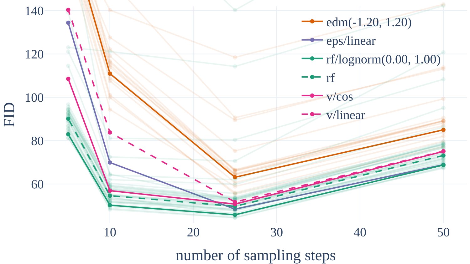
Figure 3: Rectified flows are sample efficient. Rectified Flows perform better then other formulations when sampling fewer steps. For 25 and more steps, only rf/lognorm(0.00, 1.00) remains competitive to eps/linear.
图 3:整流流的采样效率高。 采样步数较少时,整流流优于其他公式。达到 25 步及以上时,仅 rf/lognorm(0.00, 1.00) 仍能与 eps/linear 抗衡。
5.2 Improving Modality Specific Representations
5.2 改进模态特定表示
Having found a formulation in the previous section that allows rectified flow models to not only compete with established diffusion formulations such as LDM-Linear (Rombach et al., 2022) or EDM (Karras et al., 2022), but even outperforms them, we now turn to the application of our formulation to high-resolution text-to-image synthesis. Accordingly, the final performance of our algorithm depends not only on the training formulation, but also on the parameterization via a neural network and the quality of the image and text representations we use. In the following sections, we describe how we improve all these components before scaling our final method in Section 5.3.
上一节已找到一种公式,使整流流不仅能与 LDM-Linear (Rombach et al., 2022) 或 EDM (Karras et al., 2022) 等既有扩散公式竞争,甚至超过它们;我们转而把它用于高分辨率文生图。因而最终表现不仅取决于训练公式,也取决于神经网络参数化以及所用图像与文本表示的质量。以下各节说明我们如何改进这些组件,再在第 5.3 节缩放最终方法。
5.2.1 Improved Autoencoders
Latent diffusion models achieve high efficiency by operating in the latent space of a pretrained autoencoder (Rombach et al., 2022), which maps an input RGB into a lower-dimensional space . The reconstruction quality of this autoencoder provides an upper bound on the achievable image quality after latent diffusion training. Similar to Dai et al. (2023), we find that increasing the number of latent channels significantly boosts reconstruction performance, see Table 3. Intuitively, predicting latents with higher is a more difficult task, and thus models with increased capacity should be able to perform better for larger , ultimately achieving higher image quality. We confirm this hypothesis in Figure 10, where we see that the autoencoder exhibits better scaling performance in terms of sample FID. For the remainder of this paper, we thus choose .
5.2.1 改进的自编码器
潜扩散通过在预训练自编码器的潜空间中运算获得高效性 (Rombach et al., 2022):把 RGB 输入 映到更低维空间 。该自编码器的重建质量为潜扩散训练后可达的图像质量设下上界。与 Dai et al. (2023) 类似,我们发现增大潜通道数 显著提升重建表现,见表 3。直观上,预测更高 的潜表示更难,因而更大容量的模型应在更大 上表现更好,最终得到更高图像质量。图 10 印证了这一点: 的自编码器在样本 FID 上展现更好的缩放。后文因此取 。
| Metric | 4 chn | 8 chn | 16 chn |
|---|---|---|---|
| FID () | 02.41 | 01.56 | 0****1.06 |
| Perceptual Similarity () | 00.85 | 00.68 | 0****0.45 |
| SSIM () | 00.75 | 00.79 | 0****0.86 |
| PSNR () | 25.12 | 26.40 | 28.62 |
Table 3: Improved Autoencoders. Reconstruction performance metrics for different channel configurations. The downsampling factor for all models is .
| 指标 | 4 通道 | 8 通道 | 16 通道 |
|---|---|---|---|
| FID () | 02.41 | 01.56 | 0****1.06 |
| 感知相似度 () | 00.85 | 00.68 | 0****0.45 |
| SSIM () | 00.75 | 00.79 | 0****0.86 |
| PSNR () | 25.12 | 26.40 | 28.62 |
表 3:改进的自编码器。 不同通道配置下的重建指标。全部模型下采样因子 。
a space elevator, cinematic scifi art
A cheeseburger with juicy beef patties and melted cheese sits on top of a toilet that looks like a throne and stands in the middle of the royal chamber.
a hole in the floor of my bathroom with small gremlins living in it
a small office made out of car parts
This dreamlike digital art captures a vibrant, kaleidoscopic bird in a lush rainforest.
human life depicted entirely out of fractals
an origami pig on fire in the middle of a dark room with a pentagram on the floor
an old rusted robot wearing pants and a jacket riding skis in a supermarket.
smiling cartoon dog sits at a table, coffee mug on hand, as a room goes up in flames. “This is fine,” the dog assures himself.
A whimsical and creative image depicting a hybrid creature that is a mix of a waffle and a hippopotamus. This imaginative creature features the distinctive, bulky body of a hippo, but with a texture and appearance resembling a golden-brown, crispy waffle. The creature might have elements like waffle squares across its skin and a syrup-like sheen. It’s set in a surreal environment that playfully combines a natural water habitat of a hippo with elements of a breakfast table setting, possibly including oversized utensils or plates in the background. The image should evoke a sense of playful absurdity and culinary fantasy.
(图中提示示例,原文保留)
a space elevator, cinematic scifi art
A cheeseburger with juicy beef patties and melted cheese sits on top of a toilet that looks like a throne and stands in the middle of the royal chamber.
a hole in the floor of my bathroom with small gremlins living in it
a small office made out of car parts
This dreamlike digital art captures a vibrant, kaleidoscopic bird in a lush rainforest.
human life depicted entirely out of fractals
an origami pig on fire in the middle of a dark room with a pentagram on the floor
an old rusted robot wearing pants and a jacket riding skis in a supermarket.
smiling cartoon dog sits at a table, coffee mug on hand, as a room goes up in flames. “This is fine,” the dog assures himself.
A whimsical and creative image depicting a hybrid creature that is a mix of a waffle and a hippopotamus. This imaginative creature features the distinctive, bulky body of a hippo, but with a texture and appearance resembling a golden-brown, crispy waffle. The creature might have elements like waffle squares across its skin and a syrup-like sheen. It’s set in a surreal environment that playfully combines a natural water habitat of a hippo with elements of a breakfast table setting, possibly including oversized utensils or plates in the background. The image should evoke a sense of playful absurdity and culinary fantasy.
5.2.2 Improved Captions
Betker et al. (2023) demonstrated that synthetically generated captions can greatly improve text-to-image models trained at scale. This is due to the oftentimes simplistic nature of the human-generated captions that come with large-scale image datasets, which overly focus on the image subject and usually omit details describing the background or composition of the scene, or, if applicable, displayed text (Betker et al., 2023). We follow their approach and use an off-the-shelf, state-of-the-art vision-language model, CogVLM (Wang et al., 2023), to create synthetic annotations for our large-scale image dataset. As synthetic captions may cause a text-to-image model to forget about certain concepts not present in the VLM’s knowledge corpus, we use a ratio of 50 % original and 50 % synthetic captions.
5.2.2 改进的标题
Betker et al. (2023) 表明:合成生成的标题可大幅提升大规模训练的文生图模型。原因在于大规模图像数据自带的人工标题往往过于简略,过度聚焦主体,常省略背景、构图,以及(如有)图中文字的细节 (Betker et al., 2023)。我们沿用该思路,用现成的先进视觉–语言模型 CogVLM (Wang et al., 2023) 为大规模图像数据生成合成标注。由于合成标题可能使模型遗忘 VLM 知识库中未覆盖的概念,我们采用 50% 原始 + 50% 合成的比例。
To assess the effect of training on this caption mix, we train two MM-DiT models for 250k steps, one on only original captions and the other on the 50/50 mix. We evaluate the trained models using the GenEval benchmark (Ghosh et al., 2023) in Table 4. The results demonstrate that the model trained with the addition of synthetic captions clearly outperforms the model that only utilizes original captions. We thus use the 50/50 synthetic/original caption mix for the remainder of this work.
为评估该标题混合的效果,我们训练两个 的 MM-DiT 各 250k 步:其一仅用原始标题,其二用 50/50 混合。用 GenEval 基准 (Ghosh et al., 2023) 评估,见表 4。结果表明:加入合成标题的模型明显超过仅用原始标题者。后文因此沿用 50/50 合成/原始混合。
| Original Captions | 50/50 Mix | |
|---|---|---|
| success rate [%] | success rate [%] | |
| Color Attribution | 11.75 | 24.75 |
| Colors | 71.54 | 68.09 |
| Position | 06.50 | 18.00 |
| Counting | 33.44 | 41.56 |
| Single Object | 95.00 | 93.75 |
| Two Objects | 41.41 | 52.53 |
| Overall score | 43.27 | 49.78 |
Table 4: Improved Captions. Using a 50/50 mixing ratio of synthetic (via CogVLM (Wang et al., 2023)) and original captions improves text-to-image performance. Assessed via the GenEval (Ghosh et al., 2023) benchmark.
| 原始标题 | 50/50 混合 | |
|---|---|---|
| 成功率 [%] | 成功率 [%] | |
| 颜色归属 | 11.75 | 24.75 |
| 颜色 | 71.54 | 68.09 |
| 位置 | 06.50 | 18.00 |
| 计数 | 33.44 | 41.56 |
| 单物体 | 95.00 | 93.75 |
| 两物体 | 41.41 | 52.53 |
| 总分 | 43.27 | 49.78 |
表 4:改进的标题。 以 50/50 混合合成(经 CogVLM (Wang et al., 2023))与原始标题可提升文生图表现;经 GenEval (Ghosh et al., 2023) 评估。
5.2.3 Improved Text-to-Image Backbones
In this section, we compare the performance of existing transformer-based diffusion backbones with our novel multimodal transformer-based diffusion backbone, MM-DiT, as introduced in Section 4. MM-DiT is specifically designed to handle different domains, here text and image tokens, using (two) different sets of trainable model weights. More specifically, we follow the experimental setup from Section 5.1 and compare text-to-image performance on CC12M of DiT, CrossDiT (DiT but with cross-attending to the text tokens instead of sequence-wise concatenation (Chen et al., 2023)) and our MM-DiT. For MM-DiT, we compare models with two sets of weights and three sets of weights, where the latter handles the CLIP (Radford et al., 2021) and T5 (Raffel et al., 2019) tokens (c.f. Section 4) separately. Note that DiT (w/ concatenation of text and image tokens as in Section 4) can be interpreted as a special case of MM-DiT with one shared set of weights for all modalities. Finally, we consider the UViT (Hoogeboom et al., 2023) architecture as a hybrid between the widely used UNets and transformer variants.
5.2.3 改进的文生图骨干
本节把既有基于 Transformer 的扩散骨干与第 4 节引入的新型多模态扩散骨干 MM-DiT 对比。MM-DiT 专为处理不同域(此处为文本与图像 token)设计,使用(两)套不同的可训练权重。更具体地,我们沿用第 5.1 节设定,在 CC12M 上比较 DiT、CrossDiT(DiT 但对文本 token 做交叉注意力而非序列拼接 (Chen et al., 2023))与我们的 MM-DiT。对 MM-DiT,我们比较两套权重与三套权重:后者把 CLIP (Radford et al., 2021) 与 T5 (Raffel et al., 2019) token(参见第 4 节)分开处理。注意:按第 4 节拼接文本与图像 token 的 DiT,可视为全部模态共享一套权重的 MM-DiT 特例。最后,我们把 UViT (Hoogeboom et al., 2023) 视为广泛使用的 UNet 与 Transformer 变体之间的混合。
We analyze the convergence behavior of these architectures in Figure 4: Vanilla DiT underperforms UViT. The cross-attention DiT variant CrossDiT achieves better performance than UViT, although UViT seems to learn much faster initially. Our MM-DiT variant significantly outperforms the cross-attention and vanilla variants. We observe only a small gain when using three parameter sets instead of two (at the cost of increased parameter count and VRAM usage), and thus opt for the former option for the remainder of this work.
图 4 分析这些架构的收敛:原版 DiT 不及 UViT。交叉注意力变体 CrossDiT 超过 UViT,尽管 UViT 初期学得更快。我们的 MM-DiT 显著超过交叉注意力与原版变体。用三套参数相对两套仅有小幅收益(代价是参数量与显存上升),因而后文采用两套权重方案。
Figure 4: Training dynamics of model architectures. Comparative analysis of DiT, CrossDiT, UViT, and MM-DiT on CC12M, focusing on validation loss, CLIP score, and FID. Our proposed MM-DiT performs favorably across all metrics.
图 4:模型架构的训练动态。 在 CC12M 上比较 DiT、CrossDiT、UViT 与 MM-DiT 的验证损失、CLIP 分数与 FID。所提 MM-DiT 在各项指标上均表现更好。
5.3 Training at Scale
5.3 规模化训练
Before scaling up, we filter and preencode our data to ensure safe and efficient pretraining. Then, all previous considerations of diffusion formulations, architectures, and data culminate in the last section, where we scale our models up to 8B parameters.
在放大之前,我们过滤并预编码数据,以保证预训练安全且高效。随后,此前关于扩散公式、架构与数据的全部考量汇于本节:把模型扩到 8B 参数。
Pre-Training Mitigations
Training data significantly impacts a generative model’s abilities. Consequently, data filtering is effective at constraining undesirable capabilities (Nichol, 2022). Before training at sale, we filter our data for the following categories: (i) Sexual content: We use NSFW-detection models to filter for explicit content. (ii) Aesthetics: We remove images for which our rating systems predict a low score. (iii) Regurgitation: We use a cluster-based deduplication method to remove perceptual and semantic duplicates from the training data; see Section E.2.
预训练缓解措施
训练数据显著影响生成模型能力。因此,数据过滤能有效约束不良能力 (Nichol, 2022)。放大训练前,我们按以下类别过滤:(i) 色情内容:用 NSFW 检测模型过滤露骨内容。(ii) 美学:去掉评分系统预测分低的图像。(iii) 复读/回吐:用基于聚类的去重去掉感知与语义重复;见第 E.2 节。
Precomputing Image and Text Embeddings
Our model uses the output of multiple pretrained, frozen networks as inputs (autoencoder latents and text encoder representations). Since these outputs are constant during training, we precompute them once for the entire dataset. We provide a detailed discussion of our approach in Section E.1.
预计算图像与文本嵌入
模型把多个预训练、冻结网络的输出(自编码器潜表示与文本编码器表示)当作输入。这些输出在训练中恒定,我们因而对整个数据集预计算一次。详细讨论见第 E.1 节。
5.3.2 Finetuning on High Resolutions
Figure 5: Effects of QK-normalization. Normalizing the Q- and K-embeddings before calculating the attention matrix prevents the attention-logit growth instability (left), which causes the attention entropy to collapse (right) and has been previously reported in the discriminative ViT literature (Dehghani et al., 2023; Wortsman et al., 2023). In contrast with these previous works, we observe this instability in the last transformer blocks of our networks. Maximum attention logits and attention entropies are shown averaged over the last 5 blocks of a 2B (d=24) model.
5.3.2 高分辨率微调
图 5:QK 归一化的效果。 在计算注意力矩阵前对 Q、K 嵌入归一化,可防止注意力 logit 增长导致的不稳定(左),该不稳定会使注意力熵塌缩(右),此前已在判别式 ViT 文献中报告 (Dehghani et al., 2023; Wortsman et al., 2023)。与这些工作不同,我们在网络最后若干 Transformer 块中观察到该不稳定。图中最大注意力 logit 与注意力熵对 2B(d=24)模型最后 5 块取平均。
QK-Normalization
In general, we pretrain all of our models on low-resolution images of size pixels. Next, we finetune our models on higher resolutions with mixed aspect ratios (see next paragraph for details). We find that, when moving to high resolutions, mixed precision training can become unstable and the loss diverges. This can be remedied by switching to full precision training — but comes with a performance drop compared to mixed-precision training. A more efficient alternative is reported in the (discriminative) ViT literature: Dehghani et al. (2023) observe that the training of large vision transformer models diverges because the attention entropy grows uncontrollably. To avoid this, Dehghani et al. (2023) propose to normalize Q and K before the attention operation. We follow this approach and use RMSNorm (Zhang & Sennrich, 2019) with learnable scale in both streams of our MMDiT architecture for our models, see Figure 2. As demonstrated in Figure 5, the additional normalization prevents the attention logit growth instability, confirming findings by Dehghani et al. (2023) and Wortsman et al. (2023) and enables efficient training at bf16-mixed (Chen et al., 2019) precision when combined with in the AdamW (Loshchilov & Hutter, 2017) optimizer. This technique can also be applied on pretrained models that have not used qk-normalization during pretraining: The model quickly adapts to the additional normalization layers and trains more stably. Finally, we would like to point out that although this method can generally help to stabilize the training of large models, it is not a universal recipe and may need to be adapted depending on the exact training setup.
QK 归一化
一般地,我们先在 低分辨率图像上预训练全部模型,再在混合宽高比的更高分辨率上微调(细节见下段)。我们发现:进入高分辨率后,混合精度训练可能不稳、损失发散。切到全精度可缓解,但相对混合精度大约慢 。更高效的替代方案见于(判别式)ViT 文献:Dehghani et al. (2023) 观察到大视觉 Transformer 训练因注意力熵失控增长而发散;为避免这一点,他们建议在注意力前对 Q、K 归一化。我们沿用该做法,在 MMDiT 两流中使用带可学习尺度的 RMSNorm (Zhang & Sennrich, 2019),见图 2。如图 5 所示,额外归一化防止了注意力 logit 增长不稳定,印证 Dehghani et al. (2023) 与 Wortsman et al. (2023) 的发现,并在与 AdamW (Loshchilov & Hutter, 2017) 中 结合时,支持 bf16-mixed (Chen et al., 2019) 高效训练。该技术也可用于预训练时未使用 qk-归一化的模型:模型能很快适应额外归一化层并更稳地训练。最后需指出:尽管该方法通常有助于稳定大模型训练,它并非万能配方,仍须按具体训练设定调整。
Positional Encodings for Varying Aspect Ratios
After training on a fixed resolution we aim to (i) increase the resolution and resolution and (ii) enable inference with flexible aspect ratios. Since we use 2d positional frequency embeddings we have to adapt them based on the resolution. In the multi-aspect ratio setting, a direct interpolation of the embeddings as in (Dosovitskiy et al., 2020) would not reflect the side lengths correctly. Instead we use a combination of extended and interpolated position grids which are subsequently frequency embedded.
可变宽高比的位置编码
在固定 分辨率训练后,我们希望 (i) 提高分辨率,(ii) 支持灵活宽高比推理。由于使用二维位置频率嵌入,须按分辨率适配。在多宽高比设定下,像 (Dosovitskiy et al., 2020) 那样直接插值嵌入无法正确反映边长。我们改用扩展与插值相结合的位置网格,再做频率嵌入。
For a target resolution of pixels, we use bucketed sampling (NovelAI, 2022; Podell et al., 2023) such that that each batch consists of images of a homogeneous size , where . For the maximum and minimum training aspect ratios, this results in the maximum values for width, , and height, , that will be encountered. Let and be the corresponding sizes in latent space (a factor 8) after patching (a factor 2). Based on these values, we construct a vertical position grid with the values and correspondingly for the horizontal positions. We then center-crop from the resulting positional 2d grid before embedding it.
对目标分辨率 像素,我们用分桶采样 (NovelAI, 2022; Podell et al., 2023),使每个 batch 内图像尺寸齐整为 ,且 。按训练时最大与最小宽高比,得到会遇到的最大宽 与高 。令 , 为潜空间(下采样因子 8)再经 patch(因子 2)后的对应尺寸。据此构造竖直位置网格,取值为 ,水平方向同理。再从所得二维位置网格中心裁剪后嵌入。

Figure 6: Timestep shifting at higher resolutions. Top right: Human quality preference rating when applying the shifting based on Equation 23. Bottom row: A model trained and sampled with (top) and (bottom). See Section 5.3.2.
图 6:更高分辨率下的时间步平移。 右上: 按式 23 施加平移时的人类质量偏好。底行: 在 上训练并采样、(上)与 (下)的对比。见第 5.3.2 节。
Resolution-dependent shifting of timestep schedules
Intuitively, since higher resolutions have more pixels, we need more noise to destroy their signal. Assume we are working in a resolution with pixels. Now, consider a ”constant” image, i.e. one where every pixel has the value . The forward process produces , where both and . Thus, provides observations of the random variable with and in , and follows a standard normal distribution. Thus, and . We can therefore recover via , and the error between and its sample estimate has a standard deviation of (because the standard error of the mean for has deviation ). So if one already knows that the image was constant across its pixels, represents the degree of uncertainty about . For example, we immediately see that doubling the width and height leads to half the uncertainty at any given time . But, we can now map a timestep at resolution to a timestep at resolution that results in the same degree of uncertainty via the ansatz . Solving for gives
随分辨率平移时间步日程
直观上,更高分辨率像素更多,需要更多噪声才能破坏信号。设分辨率为 像素。考虑「常数」图像,即每个像素取值 。前向过程得到 ,其中 与 。于是 提供随机变量 (, 标准正态)的 次观测。故 ,。因而可用 恢复 ,而 与样本估计 之间误差的标准差为 (因 均值标准误为 )。因此,若已知 在像素上恒定, 表示对 的不确定程度。例如立即可见:宽高各加倍,则任意 上的不确定度减半。我们可用 ansatz ,把分辨率 上的时间步 映到分辨率 上具有相同不确定度的 。求解 得
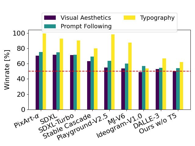
Figure 7: Human Preference Evaluation against currrent closed and open SOTA generative image models. Our 8B model compares favorable against current state-of-the-art text-to-image models when evaluated on the parti-prompts (Yu et al., 2022) across the categories visual quality, prompt following and typography generation.
图 7:相对当前闭源与开源文生图最优模型的人类偏好评估。 我们的 8B 模型在 parti-prompts (Yu et al., 2022) 上,于视觉质量、遵循提示与排版生成等类别中,与当前最优文生图模型相比表现更优。
We visualize this shifting function in Figure 6. Note that the assumption of constant images is not realistic. To find good values for the shift value during inference, we apply them to the sampling steps of a model trained at resolution and run a human preference study. The results in Figure 6 show a strong preference for samples with shifts greater than but less drastic differences among the higher shift values. In our subsequent experiments, we thus use a shift value of both during training and sampling at resolution . A qualitative comparison between samples after 8k training steps with and without such a shift can be found in Figure 6. Finally, note that Equation 23 implies a log-SNR shift of similar to (Hoogeboom et al., 2023):
图 6 可视化该平移函数。注意「常数图像」假设并不现实。为在推理时找合适的平移值 ,我们把它施加到在 上训练的模型的采样步上,并做人类偏好研究。图 6 显示:平移大于 的样本明显更受偏好,更高平移值之间差异不那么剧烈。后续实验因此在 训练与采样时取 。有无该平移、训练 8k 步后的定性对比亦见图 6。最后,式 23 蕴含与 (Hoogeboom et al., 2023) 类似的 log-SNR 平移 :
After the shifted training at resolution , we align the model using Direct Preference Optimization (DPO) as described in Appendix C.
在 上完成平移训练后,我们按附录 C 用直接偏好优化(DPO)对齐模型。
5.3.3 Results
Figure 8: Quantitative effects of scaling. We analyze the impact of model size on performance, maintaining consistent training hyperparameters throughout. An exception is depth=38, where learning rate adjustments at steps were necessary to prevent divergence. (Top) Validation loss smoothly decreases as a function of both model size and training steps for both image (columns 1 and 2) and video models (columns 3 and 4). (Bottom) Validation loss is a strong predictor of overall model performance. There is a marked correlation between validation loss and holistic image evaluation metrics, including GenEval (Ghosh et al., 2023), column 1, human preference, column 2, and T2I-CompBench (Huang et al., 2023), column 3. For video models we observe a similar correlation between validation loss and human preference, column 4. .
5.3.3 结果
图 8:缩放的定量效果。 我们分析模型规模对表现的影响,训练超参保持一致;例外是 depth=38,在 步时调整学习率以防发散。(上) 图像(第 1–2 列)与视频模型(第 3–4 列)的验证损失均随模型规模与训练步数平滑下降。(下) 验证损失是整体模型表现的强预测因子:与 GenEval (Ghosh et al., 2023)(第 1 列)、人类偏好(第 2 列)及 T2I-CompBench (Huang et al., 2023)(第 3 列)等整体图像评估强相关。视频模型上,验证损失与人类偏好(第 4 列)亦有类似相关。
In Figure 8, we examine the effect of training our MM-DiT at scale. For images, we conduct a large scaling study and train models with different numbers of parameters for 500k steps on pixels resolution using preencoded data, c.f. Section E.1, with a batch size of 4096. We train on patches (Peebles & Xie, 2023), and report validation losses on the CoCo dataset (Lin et al., 2014) every 50k steps. In particular, to reduce noise in the validation loss signal, we sample loss levels equidistant in and compute validation loss for each level separately. We then average the loss across all but the last () levels.
图 8 考察规模化训练 MM-DiT 的效果。对图像,我们做大规模缩放研究:用不同参数量的模型在 上训练 500k 步,使用预编码数据(参见第 E.1 节),batch 大小 4096。我们在 patch 上训练 (Peebles & Xie, 2023),每 50k 步在 CoCo (Lin et al., 2014) 上报验证损失。为降低验证损失噪声,我们在 上等距采样损失水平,分别计算,再对除最后一层()外全部水平取平均。
Similarly, we conduct a preliminary scaling study of our MM-DiT on videos. To this end we start from the pretrained image weights and additionally use a 2x temporal patching. We follow Blattmann et al. (2023b) and feed data to the pretrained model by collapsing the temporal into the batch axis. In each attention layer we rearrange the representation in the visual stream and add a full attention over all spatio-temporal tokens after the spatial attention operation before the final feedforward layer. Our video models are trained for 140k steps with a batch size of 512 on videos comprising 16 frames with pixels. We report validation losses on the Kinetics dataset (Carreira & Zisserman, 2018) every 5k steps. Note that our reported FLOPs for video training in Figure 8 are only FLOPs from video training and do not include the FLOPs from image pretraining.
类似地,我们对 MM-DiT 做初步视频缩放研究。从预训练图像权重出发,额外使用 2× 时间 patch。我们沿用 Blattmann et al. (2023b):把时间维塌到 batch 轴再喂入预训练模型;在每个注意力层,重排视觉流表示,并在空间注意力之后、最终前馈之前,对全部时空 token 做一次全注意力。视频模型训练 140k 步,batch 512,视频为 16 帧、 像素。每 5k 步在 Kinetics (Carreira & Zisserman, 2018) 上报验证损失。注意图 8 中视频训练的 FLOPs 仅含视频阶段,不含图像预训练。
For both the image and video domains, we observe a smooth decrease in the validation loss when increasing model size and training steps. We find the validation loss to be highly correlated to comprehensive evaluation metrics (CompBench (Huang et al., 2023), GenEval (Ghosh et al., 2023)) and to human preference. These results support the validation loss as a simple and general measure of model performance. Our results do not show saturation neither for image not for video models.
在图像与视频域,我们都观察到:增大模型与训练步数时,验证损失平滑下降。验证损失与综合评估指标(CompBench (Huang et al., 2023)、GenEval (Ghosh et al., 2023))及人类偏好高度相关。这些结果支持把验证损失当作简单且通用的表现度量。图像与视频模型均未见饱和迹象。
Figure 12 illustrates how training a larger model for longer impacts sample quality. Tab. 5 shows the results of GenEval in full. When applying the methods presented in Section 5.3.2 and increasing training image resolution, our biggest model excels in most categories and outperforms DALLE 3 (Betker et al., 2023), the current state of the art in prompt comprehension, in overall score.
图 12 展示更长时间训练更大模型如何影响样本质量。表 5 给出完整 GenEval 结果。应用第 5.3.2 节方法并提高训练分辨率后,我们最大的模型在多数类别领先,并在总分上超过当前提示理解最优的 DALL·E 3 (Betker et al., 2023)。
| All text-encoders | w/o T5 (Raffel et al., 2019) |
|---|---|
| “A burger patty, with the bottom bun and lettuce and tomatoes. ”COFFEE” written on it in mustard” | |
| “A monkey holding a sign reading ”Scaling transformer models is awesome!” | |
| “A mischievous ferret with a playful grin squeezes itself into a large glass jar, surrounded by colorful candy. The jar sits on a wooden table in a cozy kitchen, and warm sunlight filters through a nearby window” |
Figure 9: Impact of T5. We observe T5 to be important for complex prompts e.g. such involving a high degree of detail or longer spelled text (rows 2 and 3). For most prompts, however, we find that removing T5 at inference time still achieves competitive performance.
| 全部文本编码器 | 去掉 T5 (Raffel et al., 2019) |
|---|---|
| “A burger patty, with the bottom bun and lettuce and tomatoes. ”COFFEE” written on it in mustard” | |
| “A monkey holding a sign reading ”Scaling transformer models is awesome!” | |
| “A mischievous ferret with a playful grin squeezes itself into a large glass jar, surrounded by colorful candy. The jar sits on a wooden table in a cozy kitchen, and warm sunlight filters through a nearby window” |
图 9:T5 的影响。 我们观察到 T5 对复杂提示(例如细节很多或较长拼写文字,第 2–3 行)很重要。但对多数提示,推理时去掉 T5 仍可达到有竞争力的表现。
Our model outperforms current proprietary (Betker et al., 2023; ide, 2024) and open (Sauer et al., 2023; pla, 2024; Chen et al., 2023; Pernias et al., 2023) SOTA generative image models in human preference evaluation on the Parti-prompts benchmark (Yu et al., 2022) in the categories visual aesthetics, prompt following and typography generation, c.f. Figure 7. For evaluating human preference in these categories, raters were shown pairwise outputs from two models, and asked to answer the following questions: Prompt following: Which image looks more representative to the text shown above and faithfully follows it? Visual aesthetics: Given the prompt, which image is of higher-quality and aesthetically more pleasing? Typography: Which image more accurately shows/displays the text specified in the above description? More accurate spelling is preferred! Ignore other aspects.
我们的 模型在 Parti-prompts 基准 (Yu et al., 2022) 的人类偏好评估中,于视觉美学、遵循提示与排版生成等类别超过当前专有 (Betker et al., 2023; ide, 2024) 与开源 (Sauer et al., 2023; pla, 2024; Chen et al., 2023; Pernias et al., 2023) 最优图像生成模型,见图 7。评估时向评分者展示两模型成对输出,并询问:遵循提示:哪张图对上方文本更具代表性且忠实遵循?视觉美学:给定提示,哪张图质量更高、更美观?排版:哪张图更准确显示上述描述中指定的文字?拼写更准确者优先!忽略其他方面。
Lastly, Table 6 highlights an intriguing result: not only do bigger models perform better, they also require fewer steps to reach their peak performance.
最后,表 6 给出一个有意思的结果:更大的模型不仅表现更好,达到峰值表现所需的步数也更少。
| Model | Overall | Objects | Counting | Colors | Position | Color | |
|---|---|---|---|---|---|---|---|
| Single | Two | Attribution | |||||
| minDALL-E | 0.23 | 0.73 | 0.11 | 0.12 | 0.37 | 0.02 | 0.01 |
| SD v1.5 | 0.43 | 0.97 | 0.38 | 0.35 | 0.76 | 0.04 | 0.06 |
| PixArt-alpha | 0.48 | 0.98 | 0.50 | 0.44 | 0.80 | 0.08 | 0.07 |
| SD v2.1 | 0.50 | 0.98 | 0.51 | 0.44 | 0.85 | 0.07 | 0.17 |
| DALL-E 2 | 0.52 | 0.94 | 0.66 | 0.49 | 0.77 | 0.10 | 0.19 |
| SDXL | 0.55 | 0.98 | 0.74 | 0.39 | 0.85 | 0.15 | 0.23 |
| SDXL Turbo | 0.55 | 1.00 | 0.72 | 0.49 | 0.80 | 0.10 | 0.18 |
| IF-XL | 0.61 | 0.97 | 0.74 | 0.66 | 0.81 | 0.13 | 0.35 |
| DALL-E 3 | 0.67 | 0.96 | 0.87 | 0.47 | 0.83 | 0.43 | 0.45 |
| Ours (depth=18), | 0.58 | 0.97 | 0.72 | 0.52 | 0.78 | 0.16 | 0.34 |
| Ours (depth=24), | 0.62 | 0.98 | 0.74 | 0.63 | 0.67 | 0.34 | 0.36 |
| Ours (depth=30), | 0.64 | 0.96 | 0.80 | 0.65 | 0.73 | 0.33 | 0.37 |
| Ours (depth=38), | 0.68 | 0.98 | 0.84 | 0.66 | 0.74 | 0.40 | 0.43 |
| Ours (depth=38), w/DPO | 0.71 | 0.98 | 0.89 | 0.73 | 0.83 | 0.34 | 0.47 |
| Ours (depth=38), w/DPO | 0.74 | 0.99 | 0.94 | 0.72 | 0.89 | 0.33 | 0.60 |
Table 5: GenEval comparisons. Our largest model (depth=38) outperforms all current open models and DALLE-3 (Betker et al., 2023) on GenEval (Ghosh et al., 2023). We highlight the best, second best, and third best entries. For DPO, see Appendix C.
| 模型 | 总分 | 物体 | 计数 | 颜色 | 位置 | 颜色归属 | |
|---|---|---|---|---|---|---|---|
| 单 | 双 | ||||||
| minDALL-E | 0.23 | 0.73 | 0.11 | 0.12 | 0.37 | 0.02 | 0.01 |
| SD v1.5 | 0.43 | 0.97 | 0.38 | 0.35 | 0.76 | 0.04 | 0.06 |
| PixArt-alpha | 0.48 | 0.98 | 0.50 | 0.44 | 0.80 | 0.08 | 0.07 |
| SD v2.1 | 0.50 | 0.98 | 0.51 | 0.44 | 0.85 | 0.07 | 0.17 |
| DALL-E 2 | 0.52 | 0.94 | 0.66 | 0.49 | 0.77 | 0.10 | 0.19 |
| SDXL | 0.55 | 0.98 | 0.74 | 0.39 | 0.85 | 0.15 | 0.23 |
| SDXL Turbo | 0.55 | 1.00 | 0.72 | 0.49 | 0.80 | 0.10 | 0.18 |
| IF-XL | 0.61 | 0.97 | 0.74 | 0.66 | 0.81 | 0.13 | 0.35 |
| DALL-E 3 | 0.67 | 0.96 | 0.87 | 0.47 | 0.83 | 0.43 | 0.45 |
| Ours (depth=18), | 0.58 | 0.97 | 0.72 | 0.52 | 0.78 | 0.16 | 0.34 |
| Ours (depth=24), | 0.62 | 0.98 | 0.74 | 0.63 | 0.67 | 0.34 | 0.36 |
| Ours (depth=30), | 0.64 | 0.96 | 0.80 | 0.65 | 0.73 | 0.33 | 0.37 |
| Ours (depth=38), | 0.68 | 0.98 | 0.84 | 0.66 | 0.74 | 0.40 | 0.43 |
| Ours (depth=38), w/DPO | 0.71 | 0.98 | 0.89 | 0.73 | 0.83 | 0.34 | 0.47 |
| Ours (depth=38), w/DPO | 0.74 | 0.99 | 0.94 | 0.72 | 0.89 | 0.33 | 0.60 |
表 5:GenEval 对比。 我们最大的模型(depth=38)在 GenEval (Ghosh et al., 2023) 上超过全部当前开源模型与 DALL·E 3 (Betker et al., 2023)。标出最优、次优与第三优。DPO 见附录 C。
| relative CLIP score decrease [%] | ||||
|---|---|---|---|---|
| 5/50 steps | 10/50 steps | 20/50 steps | path length | |
| depth=15 | 4.30 | 0.86 | 0.21 | 191.13 |
| depth=30 | 3.59 | 0.70 | 0.24 | 187.96 |
| depth=38 | 2.71 | 0.14 | 0.08 | 185.96 |
Table 6: Impact of model size on sampling efficiency. The table shows the relative performance decrease relative to CLIP scores evaluated using 50 sampling steps at a fixed seed. Larger models can be sampled using fewer steps, which we attribute to increased robustness and better fitting the straight-path objective of rectified flow models, resulting in shorter path lengths. Path length is calculated by summing up over 50 steps.
| 相对 CLIP 分数下降 [%] | ||||
|---|---|---|---|---|
| 5/50 步 | 10/50 步 | 20/50 步 | 路径长度 | |
| depth=15 | 4.30 | 0.86 | 0.21 | 191.13 |
| depth=30 | 3.59 | 0.70 | 0.24 | 187.96 |
| depth=38 | 2.71 | 0.14 | 0.08 | 185.96 |
表 6:模型规模对采样效率的影响。 相对固定种子下 50 采样步的 CLIP 分数,表中给出相对性能下降。更大模型可用更少步数采样,我们将其归因于稳健性增强,以及更好地拟合整流流的直线路径目标,从而路径更短。路径长度按 50 步累加 。
Flexible Text Encoders
While the main motivation for using multiple text-encoders is boosting the overall model performance (Balaji et al., 2022), we now show that this choice additionally increases the flexibility of our MM-DiT-based rectified flow during inference. As described in Section B.3 we train our model with three text encoders, with an individual drop-out rate of 46.3%. Hence, at inference time, we can use an arbitrary subset of all three text encoders. This offers means for trading off model performance for improved memory efficiency, which is particularly relevant for the 4.7B parameters of T5-XXL (Raffel et al., 2019) that require significant amounts of VRAM. Interestingly, we observe limited performance drops when using only the two CLIP-based text-encoders for the text prompts and replacing the T5 embeddings by zeros. We provide a qualitative visualization in Figure 9. Only for complex prompts involving either highly detailed descriptions of a scene or larger amounts of written text do we find significant performance gains when using all three text-encoders. These observations are also verified in the human preference evaluation results in Figure 7 (Ours w/o T5). Removing T5 has no effect on aesthetic quality ratings ( win rate), and only a small impact on prompt adherence ( win rate), whereas its contribution to the capabilities of generating written text are more significant ( win rate).
灵活的文本编码器
使用多个文本编码器的主要动机是提升整体表现 (Balaji et al., 2022);我们进一步表明:该选择也增加基于 MM-DiT 的整流流在推理时的灵活性。如第 B.3 节所述,我们用三个文本编码器训练,各自 dropout 率 46.3%。因而推理时可任选三者的子集。这提供了在模型表现与显存效率之间折中的手段,对需要大量显存的 4.7B 参数 T5-XXL (Raffel et al., 2019) 尤其相关。有意思的是:仅用两个基于 CLIP 的文本编码器、把 T5 嵌入换成零时,性能下降有限。定性可视化见图 9。仅当提示高度复杂——场景细节极多或书面文字量较大——时,三个编码器才带来显著收益。图 7 的人类偏好亦印证(Ours w/o T5):去掉 T5 对美学评分无影响(胜率 50%),对遵循提示影响很小(46%),对生成书面文字的能力贡献更大(38%)。
6 Conclusion
6 结论
In this work, we presented a scaling analysis of rectified flow models for text-to-image synthesis. We proposed a novel timestep sampling for rectified flow training that improves over previous diffusion training formulations for latent diffusion models and retains the favourable properties of rectified flows in the few-step sampling regime. We also demonstrated the advantages of our transformer-based MM-DiT architecture that takes the multi-modal nature of the text-to-image task into account. Finally, we performed a scaling study of this combination up to a model size of 8B parameters and training FLOPs. We showed that validation loss improvements correlate with both existing text-to-image benchmarks as well as human preference evaluations. This, in combination with our improvements in generative modeling and scalable, multimodal architectures achieves performance that is competitive with state-of-the-art proprietary models. The scaling trend shows no signs of saturation, which makes us optimistic that we can continue to improve the performance of our models in the future.
本文对文生图的整流流模型做了缩放分析。我们提出一种新的整流流训练时间步采样,相对此前潜扩散的训练公式有所提升,并在少步采样下保留整流流的有利性质。我们也展示了面向文生图多模态特性的 Transformer 架构 MM-DiT 的优势。最后,我们把该组合缩放到 8B 参数与 训练 FLOPs,并表明验证损失的改进与既有文生图基准及人类偏好评估相关。结合生成建模与可扩展多模态架构上的改进,我们达到与当前专有最优模型相当的表现。缩放趋势未见饱和,使我们乐观地认为未来仍可继续提升。
Broader Impact
更广泛的影响
This paper presents work whose goal is to advance the field of machine learning in general and image synthesis in particular. There are many potential societal consequences of our work, none of which we feel must be specifically highlighted here. For an extensive discussion of the general ramifications of diffusion models, we point interested readers towards (Po et al., 2023).
本文工作旨在推进机器学习整体与图像合成领域。潜在社会影响很多,我们不认为有必须在此单独强调的条目。关于扩散模型一般性后果的详尽讨论,请参见 (Po et al., 2023)。
References
参考文献
Supplementary
补充材料
Detailed pen and ink drawing of a happy pig butcher selling meat in its shop.
a massive alien space ship that is shaped like a pretzel.
A kangaroo holding a beer, wearing ski goggles and passionately singing silly songs.
An entire universe inside a bottle sitting on the shelf at walmart on sale.
A cheesburger surfing the vibe wave at night
A swamp ogre with a pearl earring by Johannes Vermeer
A car made out of vegetables.
heat death of the universe, line art
A crab made of cheese on a plate
Dystopia of thousand of workers picking cherries and feeding them into a machine that runs on steam and is as large as a skyscraper. Written on the side of the machine: ”SD3 Paper”
translucent pig, inside is a smaller pig.
Film still of a long-legged cute big-eye anthropomorphic cheeseburger wearing sneakers relaxing on the couch in a sparsely decorated living room.
(补充图中的英文提示示例,原文保留)
Detailed pen and ink drawing of a happy pig butcher selling meat in its shop.
a massive alien space ship that is shaped like a pretzel.
A kangaroo holding a beer, wearing ski goggles and passionately singing silly songs.
An entire universe inside a bottle sitting on the shelf at walmart on sale.
A cheesburger surfing the vibe wave at night
A swamp ogre with a pearl earring by Johannes Vermeer
A car made out of vegetables.
heat death of the universe, line art
A crab made of cheese on a plate
Dystopia of thousand of workers picking cherries and feeding them into a machine that runs on steam and is as large as a skyscraper. Written on the side of the machine: ”SD3 Paper”
translucent pig, inside is a smaller pig.
Film still of a long-legged cute big-eye anthropomorphic cheeseburger wearing sneakers relaxing on the couch in a sparsely decorated living room.
detailed pen and ink drawing of a massive complex alien space ship above a farm in the middle of nowhere.
photo of a bear wearing a suit and tophat in a river in the middle of a forest holding a sign that says ”I cant bear it”.
tilt shift aerial photo of a cute city made of sushi on a wooden table in the evening.
dark high contrast render of a psychedelic tree of life illuminating dust in a mystical cave.
an anthropomorphic fractal person behind the counter at a fractal themed restaurant.
beautiful oil painting of a steamboat in a river in the afternoon. On the side of the river is a large brick building with a sign on top that says S̈D3.̈
an anthopomorphic pink donut with a mustache and cowboy hat standing by a log cabin in a forest with an old 1970s orange truck in the driveway
fox sitting in front of a computer in a messy room at night. On the screen is a 3d modeling program with a line render of a zebra.
(补充图中的英文提示示例,原文保留)
detailed pen and ink drawing of a massive complex alien space ship above a farm in the middle of nowhere.
photo of a bear wearing a suit and tophat in a river in the middle of a forest holding a sign that says ”I cant bear it”.
tilt shift aerial photo of a cute city made of sushi on a wooden table in the evening.
dark high contrast render of a psychedelic tree of life illuminating dust in a mystical cave.
an anthropomorphic fractal person behind the counter at a fractal themed restaurant.
beautiful oil painting of a steamboat in a river in the afternoon. On the side of the river is a large brick building with a sign on top that says S̈D3.̈
an anthopomorphic pink donut with a mustache and cowboy hat standing by a log cabin in a forest with an old 1970s orange truck in the driveway
fox sitting in front of a computer in a messy room at night. On the screen is a 3d modeling program wi
ide (2024) Ideogram v1.0 announcement, 2024. URL https://about.ideogram.ai/1.0 .
pla (2024) Playground v2.5 announcement, 2024. URL https://blog.playgroundai.com/playground-v2-5/ .
Albergo & Vanden-Eijnden (2022) Albergo, M. S. and Vanden-Eijnden, E. Building normalizing flows with stochastic interpolants, 2022.
Atchison & Shen (1980) Atchison, J. and Shen, S. M. Logistic-normal distributions: Some properties and uses. Biometrika , 67(2):261–272, 1980.
autofaiss (2023) autofaiss. autofaiss, 2023. URL https://github.com/criteo/autofaiss .
Balaji et al. (2022) Balaji, Y., Nah, S., Huang, X., Vahdat, A., Song, J., Zhang, Q., Kreis, K., Aittala, M., Aila, T., Laine, S., Catanzaro, B., Karras, T., and Liu, M.-Y. ediff-i: Text-to-image diffusion models with an ensemble of expert denoisers, 2022.
Betker et al. (2023) Betker, J., Goh, G., Jing, L., Brooks, T., Wang, J., Li, L., Ouyang, L., Zhuang, J., Lee, J., Guo, Y., et al. Improving image generation with better captions. Computer Science. https://cdn. openai. com/papers/dall-e-3. pdf , 2(3), 2023.
Blattmann et al. (2023a) Blattmann, A., Dockhorn, T., Kulal, S., Mendelevitch, D., Kilian, M., Lorenz, D., Levi, Y., English, Z., Voleti, V., Letts, A., et al. Stable video diffusion: Scaling latent video diffusion models to large datasets. arXiv preprint arXiv:2311.15127 , 2023a.
Blattmann et al. (2023b) Blattmann, A., Rombach, R., Ling, H., Dockhorn, T., Kim, S. W., Fidler, S., and Kreis, K. Align your latents: High-resolution video synthesis with latent diffusion models, 2023b.
Brooks et al. (2023) Brooks, T., Holynski, A., and Efros, A. A. Instructpix2pix: Learning to follow image editing instructions. In Proceedings of the IEEE/CVF Conference on Computer Vision and Pattern Recognition , pp. 18392–18402, 2023.
Carlini et al. (2023) Carlini, N., Hayes, J., Nasr, M., Jagielski, M., Sehwag, V., Tramer, F., Balle, B., Ippolito, D., and Wallace, E. Extracting training data from diffusion models. In 32nd USENIX Security Symposium (USENIX Security 23) , pp. 5253–5270, 2023.
Carreira & Zisserman (2018) Carreira, J. and Zisserman, A. Quo vadis, action recognition? a new model and the kinetics dataset, 2018.
Changpinyo et al. (2021) Changpinyo, S., Sharma, P. K., Ding, N., and Soricut, R. Conceptual 12m: Pushing web-scale image-text pre-training to recognize long-tail visual concepts. 2021 IEEE/CVF Conference on Computer Vision and Pattern Recognition (CVPR) , pp. 3557–3567, 2021. URL https://api.semanticscholar.org/CorpusID:231951742 .
Chen et al. (2019) Chen, D., Chou, C., Xu, Y., and Hseu, J. Bfloat16: The secret to high performance on cloud tpus, 2019. URL https://cloud.google.com/blog/products/ai-machine-learning/bfloat16-the-secret-to-high-performance-on-cloud-tpus?hl=en .
Chen et al. (2023) Chen, J., Yu, J., Ge, C., Yao, L., Xie, E., Wu, Y., Wang, Z., Kwok, J., Luo, P., Lu, H., and Li, Z. Pixart-a: Fast training of diffusion transformer for photorealistic text-to-image synthesis, 2023.
Chen et al. (2018) Chen, T. Q., Rubanova, Y., Bettencourt, J., and Duvenaud, D. K. Neural ordinary differential equations. In Neural Information Processing Systems , 2018. URL https://api.semanticscholar.org/CorpusID:49310446 .
Cherti et al. (2023) Cherti, M., Beaumont, R., Wightman, R., Wortsman, M., Ilharco, G., Gordon, C., Schuhmann, C., Schmidt, L., and Jitsev, J. Reproducible scaling laws for contrastive language-image learning. In 2023 IEEE/CVF Conference on Computer Vision and Pattern Recognition (CVPR) . IEEE, 2023. doi: 10.1109/cvpr52729.2023.00276 . URL http://dx.doi.org/10.1109/CVPR52729.2023.00276 .
Dai et al. (2023) Dai, X., Hou, J., Ma, C.-Y., Tsai, S., Wang, J., Wang, R., Zhang, P., Vandenhende, S., Wang, X., Dubey, A., Yu, M., Kadian, A., Radenovic, F., Mahajan, D., Li, K., Zhao, Y., Petrovic, V., Singh, M. K., Motwani, S., Wen, Y., Song, Y., Sumbaly, R., Ramanathan, V., He, Z., Vajda, P., and Parikh, D. Emu: Enhancing image generation models using photogenic needles in a haystack, 2023.
Dao et al. (2023) Dao, Q., Phung, H., Nguyen, B., and Tran, A. Flow matching in latent space, 2023.
Dehghani et al. (2023) Dehghani, M., Djolonga, J., Mustafa, B., Padlewski, P., Heek, J., Gilmer, J., Steiner, A., Caron, M., Geirhos, R., Alabdulmohsin, I., Jenatton, R., Beyer, L., Tschannen, M., Arnab, A., Wang, X., Riquelme, C., Minderer, M., Puigcerver, J., Evci, U., Kumar, M., van Steenkiste, S., Elsayed, G. F., Mahendran, A., Yu, F., Oliver, A., Huot, F., Bastings, J., Collier, M. P., Gritsenko, A., Birodkar, V., Vasconcelos, C., Tay, Y., Mensink, T., Kolesnikov, A., Pavetić, F., Tran, D., Kipf, T., Lučić, M., Zhai, X., Keysers, D., Harmsen, J., and Houlsby, N. Scaling vision transformers to 22 billion parameters, 2023.
Dhariwal & Nichol (2021) Dhariwal, P. and Nichol, A. Diffusion models beat gans on image synthesis, 2021.
Dockhorn et al. (2021) Dockhorn, T., Vahdat, A., and Kreis, K. Score-based generative modeling with critically-damped langevin diffusion. arXiv preprint arXiv:2112.07068 , 2021.
Dockhorn et al. (2022) Dockhorn, T., Vahdat, A., and Kreis, K. Genie: Higher-order denoising diffusion solvers, 2022.
Dosovitskiy et al. (2020) Dosovitskiy, A., Beyer, L., Kolesnikov, A., Weissenborn, D., Zhai, X., Unterthiner, T., Dehghani, M., Minderer, M., Heigold, G., Gelly, S., et al. An image is worth 16x16 words: Transformers for image recognition at scale. ICLR , 2020.
Esser et al. (2023) Esser, P., Chiu, J., Atighehchian, P., Granskog, J., and Germanidis, A. Structure and content-guided video synthesis with diffusion models, 2023.
Euler (1768) Euler, L. Institutionum calculi integralis . Number Bd. 1 in Institutionum calculi integralis. imp. Acad. imp. Saènt., 1768. URL https://books.google.de/books?id=Vg8OAAAAQAAJ .
Fischer et al. (2023) Fischer, J. S., Gui, M., Ma, P., Stracke, N., Baumann, S. A., and Ommer, B. Boosting latent diffusion with flow matching. arXiv preprint arXiv:2312.07360 , 2023.
Ghosh et al. (2023) Ghosh, D., Hajishirzi, H., and Schmidt, L. Geneval: An object-focused framework for evaluating text-to-image alignment. arXiv preprint arXiv:2310.11513 , 2023.
Gupta et al. (2023) Gupta, A., Yu, L., Sohn, K., Gu, X., Hahn, M., Fei-Fei, L., Essa, I., Jiang, L., and Lezama, J. Photorealistic video generation with diffusion models, 2023.
Hessel et al. (2021) Hessel, J., Holtzman, A., Forbes, M., Le Bras, R., and Choi, Y. Clipscore: A reference-free evaluation metric for image captioning. In Proceedings of the 2021 Conference on Empirical Methods in Natural Language Processing . Association for Computational Linguistics, 2021. doi: 10.18653/v1/2021.emnlp-main.595 . URL http://dx.doi.org/10.18653/v1/2021.emnlp-main.595 .
Heusel et al. (2017) Heusel, M., Ramsauer, H., Unterthiner, T., Nessler, B., and Hochreiter, S. Gans trained by a two time-scale update rule converge to a local nash equilibrium, 2017.
Ho & Salimans (2022) Ho, J. and Salimans, T. Classifier-free diffusion guidance, 2022.
Ho et al. (2020) Ho, J., Jain, A., and Abbeel, P. Denoising diffusion probabilistic models, 2020.
Ho et al. (2022) Ho, J., Chan, W., Saharia, C., Whang, J., Gao, R., Gritsenko, A., Kingma, D. P., Poole, B., Norouzi, M., Fleet, D. J., and Salimans, T. Imagen video: High definition video generation with diffusion models, 2022.
Hoogeboom et al. (2023) Hoogeboom, E., Heek, J., and Salimans, T. Simple diffusion: End-to-end diffusion for high resolution images, 2023.
Huang et al. (2023) Huang, K., Sun, K., Xie, E., Li, Z., and Liu, X. T2i-compbench: A comprehensive benchmark for open-world compositional text-to-image generation. arXiv preprint arXiv:2307.06350 , 2023.
Hyvärinen (2005) Hyvärinen, A. Estimation of non-normalized statistical models by score matching. J. Mach. Learn. Res. , 6:695–709, 2005. URL https://api.semanticscholar.org/CorpusID:1152227 .
Kaplan et al. (2020) Kaplan, J., McCandlish, S., Henighan, T., Brown, T. B., Chess, B., Child, R., Gray, S., Radford, A., Wu, J., and Amodei, D. Scaling laws for neural language models, 2020.
Karras et al. (2022) Karras, T., Aittala, M., Aila, T., and Laine, S. Elucidating the design space of diffusion-based generative models. ArXiv , abs/2206.00364, 2022. URL https://api.semanticscholar.org/CorpusID:249240415 .
Karras et al. (2023) Karras, T., Aittala, M., Lehtinen, J., Hellsten, J., Aila, T., and Laine, S. Analyzing and improving the training dynamics of diffusion models. arXiv preprint arXiv:2312.02696 , 2023.
Kingma & Gao (2023) Kingma, D. P. and Gao, R. Understanding diffusion objectives as the elbo with simple data augmentation. In Thirty-seventh Conference on Neural Information Processing Systems , 2023.
Lee et al. (2021) Lee, K., Ippolito, D., Nystrom, A., Zhang, C., Eck, D., Callison-Burch, C., and Carlini, N. Deduplicating training data makes language models better. arXiv preprint arXiv:2107.06499 , 2021.
Lee et al. (2023) Lee, S., Kim, B., and Ye, J. C. Minimizing trajectory curvature of ode-based generative models, 2023.
Lin et al. (2024) Lin, S., Liu, B., Li, J., and Yang, X. Common diffusion noise schedules and sample steps are flawed. In Proceedings of the IEEE/CVF Winter Conference on Applications of Computer Vision , pp. 5404–5411, 2024.
Lin et al. (2014) Lin, T.-Y., Maire, M., Belongie, S., Hays, J., Perona, P., Ramanan, D., Dollár, P., and Zitnick, C. L. Microsoft COCO: Common Objects in Context , pp. 740–755. Springer International Publishing, 2014. ISBN 9783319106021. doi: 10.1007/978-3-319-10602-1_48 . URL http://dx.doi.org/10.1007/978-3-319-10602-1_48 .
Lipman et al. (2023) Lipman, Y., Chen, R. T. Q., Ben-Hamu, H., Nickel, M., and Le, M. Flow matching for generative modeling. In The Eleventh International Conference on Learning Representations , 2023. URL https://openreview.net/forum?id=PqvMRDCJT9t .
Liu et al. (2022) Liu, X., Gong, C., and Liu, Q. Flow straight and fast: Learning to generate and transfer data with rectified flow, 2022.
Liu et al. (2023) Liu, X., Zhang, X., Ma, J., Peng, J., and Liu, Q. Instaflow: One step is enough for high-quality diffusion-based text-to-image generation, 2023.
Loshchilov & Hutter (2017) Loshchilov, I. and Hutter, F. Fixing weight decay regularization in adam. ArXiv , abs/1711.05101, 2017. URL https://api.semanticscholar.org/CorpusID:3312944 .
Lu et al. (2023) Lu, C., Zhou, Y., Bao, F., Chen, J., Li, C., and Zhu, J. Dpm-solver++: Fast solver for guided sampling of diffusion probabilistic models, 2023.
Ma et al. (2024) Ma, N., Goldstein, M., Albergo, M. S., Boffi, N. M., Vanden-Eijnden, E., and Xie, S. Sit: Exploring flow and diffusion-based generative models with scalable interpolant transformers, 2024.
Nichol (2022) Nichol, A. Dall-e 2 pre-training mitigations. https://openai.com/research/dall-e-2-pre-training-mitigations , 2022.
Nichol & Dhariwal (2021) Nichol, A. and Dhariwal, P. Improved denoising diffusion probabilistic models, 2021.
NovelAI (2022) NovelAI. Novelai improvements on stable diffusion, 2022. URL https://blog.novelai.net/novelai-improvements-on-stable-diffusion-e10d38db82ac .
Peebles & Xie (2023) Peebles, W. and Xie, S. Scalable diffusion models with transformers. In 2023 IEEE/CVF International Conference on Computer Vision (ICCV) . IEEE, 2023. doi: 10.1109/iccv51070.2023.00387 . URL http://dx.doi.org/10.1109/ICCV51070.2023.00387 .
Pernias et al. (2023) Pernias, P., Rampas, D., Richter, M. L., Pal, C. J., and Aubreville, M. Wuerstchen: An efficient architecture for large-scale text-to-image diffusion models, 2023.
Pizzi et al. (2022) Pizzi, E., Roy, S. D., Ravindra, S. N., Goyal, P., and Douze, M. A self-supervised descriptor for image copy detection. In Proceedings of the IEEE/CVF Conference on Computer Vision and Pattern Recognition , pp. 14532–14542, 2022.
Po et al. (2023) Po, R., Yifan, W., Golyanik, V., Aberman, K., Barron, J. T., Bermano, A. H., Chan, E. R., Dekel, T., Holynski, A., Kanazawa, A., et al. State of the art on diffusion models for visual computing. arXiv preprint arXiv:2310.07204 , 2023.
Podell et al. (2023) Podell, D., English, Z., Lacey, K., Blattmann, A., Dockhorn, T., Müller, J., Penna, J., and Rombach, R. Sdxl: Improving latent diffusion models for high-resolution image synthesis, 2023.
Pooladian et al. (2023) Pooladian, A.-A., Ben-Hamu, H., Domingo-Enrich, C., Amos, B., Lipman, Y., and Chen, R. T. Q. Multisample flow matching: Straightening flows with minibatch couplings, 2023.
Radford et al. (2021) Radford, A., Kim, J. W., Hallacy, C., Ramesh, A., Goh, G., Agarwal, S., Sastry, G., Askell, A., Mishkin, P., Clark, J., Krueger, G., and Sutskever, I. Learning transferable visual models from natural language supervision, 2021.
Rafailov et al. (2023) Rafailov, R., Sharma, A., Mitchell, E., Ermon, S., Manning, C. D., and Finn, C. Direct Preference Optimization: Your Language Model is Secretly a Reward Model. arXiv:2305.18290 , 2023.
Raffel et al. (2019) Raffel, C., Shazeer, N., Roberts, A., Lee, K., Narang, S., Matena, M., Zhou, Y., Li, W., and Liu, P. J. Exploring the limits of transfer learning with a unified text-to-text transformer, 2019.
Ramesh et al. (2022) Ramesh, A., Dhariwal, P., Nichol, A., Chu, C., and Chen, M. Hierarchical text-conditional image generation with clip latents, 2022.
Rombach et al. (2022) Rombach, R., Blattmann, A., Lorenz, D., Esser, P., and Ommer, B. High-resolution image synthesis with latent diffusion models. In 2022 IEEE/CVF Conference on Computer Vision and Pattern Recognition (CVPR) . IEEE, 2022. doi: 10.1109/cvpr52688.2022.01042 . URL http://dx.doi.org/10.1109/CVPR52688.2022.01042 .
Ronneberger et al. (2015) Ronneberger, O., Fischer, P., and Brox, T. U-Net: Convolutional Networks for Biomedical Image Segmentation , pp. 234–241. Springer International Publishing, 2015. ISBN 9783319245744. doi: 10.1007/978-3-319-24574-4_28 . URL http://dx.doi.org/10.1007/978-3-319-24574-4_28 .
Russakovsky et al. (2014) Russakovsky, O., Deng, J., Su, H., Krause, J., Satheesh, S., Ma, S., Huang, Z., Karpathy, A., Khosla, A., Bernstein, M. S., Berg, A. C., and Fei-Fei, L. Imagenet large scale visual recognition challenge. International Journal of Computer Vision , 115:211 – 252, 2014. URL https://api.semanticscholar.org/CorpusID:2930547 .
Saharia et al. (2022a) Saharia, C., Chan, W., Chang, H., Lee, C., Ho, J., Salimans, T., Fleet, D., and Norouzi, M. Palette: Image-to-image diffusion models. In ACM SIGGRAPH 2022 Conference Proceedings , pp. 1–10, 2022a.
Saharia et al. (2022b) Saharia, C., Chan, W., Saxena, S., Li, L., Whang, J., Denton, E., Ghasemipour, S. K. S., Ayan, B. K., Mahdavi, S. S., Lopes, R. G., Salimans, T., Ho, J., Fleet, D. J., and Norouzi, M. Photorealistic text-to-image diffusion models with deep language understanding, 2022b.
Saharia et al. (2022c) Saharia, C., Ho, J., Chan, W., Salimans, T., Fleet, D. J., and Norouzi, M. Image super-resolution via iterative refinement. IEEE Transactions on Pattern Analysis and Machine Intelligence , 45(4):4713–4726, 2022c.
Sauer et al. (2021) Sauer, A., Chitta, K., Müller, J., and Geiger, A. Projected gans converge faster. Advances in Neural Information Processing Systems , 2021.
Sauer et al. (2023) Sauer, A., Lorenz, D., Blattmann, A., and Rombach, R. Adversarial diffusion distillation. arXiv preprint arXiv:2311.17042 , 2023.
Sheynin et al. (2023) Sheynin, S., Polyak, A., Singer, U., Kirstain, Y., Zohar, A., Ashual, O., Parikh, D., and Taigman, Y. Emu edit: Precise image editing via recognition and generation tasks. arXiv preprint arXiv:2311.10089 , 2023.
Singer et al. (2022) Singer, U., Polyak, A., Hayes, T., Yin, X., An, J., Zhang, S., Hu, Q., Yang, H., Ashual, O., Gafni, O., Parikh, D., Gupta, S., and Taigman, Y. Make-a-video: Text-to-video generation without text-video data, 2022.
Sohl-Dickstein et al. (2015) Sohl-Dickstein, J. N., Weiss, E. A., Maheswaranathan, N., and Ganguli, S. Deep unsupervised learning using nonequilibrium thermodynamics. ArXiv , abs/1503.03585, 2015. URL https://api.semanticscholar.org/CorpusID:14888175 .
Somepalli et al. (2023a) Somepalli, G., Singla, V., Goldblum, M., Geiping, J., and Goldstein, T. Diffusion art or digital forgery? investigating data replication in diffusion models. In Proceedings of the IEEE/CVF Conference on Computer Vision and Pattern Recognition , pp. 6048–6058, 2023a.
Somepalli et al. (2023b) Somepalli, G., Singla, V., Goldblum, M., Geiping, J., and Goldstein, T. Understanding and mitigating copying in diffusion models. arXiv preprint arXiv:2305.20086 , 2023b.
Song et al. (2022) Song, J., Meng, C., and Ermon, S. Denoising diffusion implicit models, 2022.
Song & Ermon (2020) Song, Y. and Ermon, S. Generative modeling by estimating gradients of the data distribution, 2020.
Song et al. (2020) Song, Y., Sohl-Dickstein, J. N., Kingma, D. P., Kumar, A., Ermon, S., and Poole, B. Score-based generative modeling through stochastic differential equations. ArXiv , abs/2011.13456, 2020. URL https://api.semanticscholar.org/CorpusID:227209335 .
Tong et al. (2023) Tong, A., Malkin, N., Huguet, G., Zhang, Y., Rector-Brooks, J., Fatras, K., Wolf, G., and Bengio, Y. Improving and generalizing flow-based generative models with minibatch optimal transport, 2023.
Vaswani et al. (2017) Vaswani, A., Shazeer, N., Parmar, N., Uszkoreit, J., Jones, L., Gomez, A. N., Kaiser, L., and Polosukhin, I. Attention is all you need, 2017.
Villani (2008) Villani, C. Optimal transport: Old and new. 2008. URL https://api.semanticscholar.org/CorpusID:118347220 .
Vincent (2011) Vincent, P. A connection between score matching and denoising autoencoders. Neural Computation , 23:1661–1674, 2011. URL https://api.semanticscholar.org/CorpusID:5560643 .
Wallace et al. (2023) Wallace, B., Dang, M., Rafailov, R., Zhou, L., Lou, A., Purushwalkam, S., Ermon, S., Xiong, C., Joty, S., and Naik, N. Diffusion Model Alignment Using Direct Preference Optimization. arXiv:2311.12908 , 2023.
Wang et al. (2023) Wang, W., Lv, Q., Yu, W., Hong, W., Qi, J., Wang, Y., Ji, J., Yang, Z., Zhao, L., Song, X., et al. Cogvlm: Visual expert for pretrained language models. arXiv preprint arXiv:2311.03079 , 2023.
Wortsman et al. (2023) Wortsman, M., Liu, P. J., Xiao, L., Everett, K., Alemi, A., Adlam, B., Co-Reyes, J. D., Gur, I., Kumar, A., Novak, R., Pennington, J., Sohl-dickstein, J., Xu, K., Lee, J., Gilmer, J., and Kornblith, S. Small-scale proxies for large-scale transformer training instabilities, 2023.
Yu et al. (2022) Yu, J., Xu, Y., Koh, J. Y., Luong, T., Baid, G., Wang, Z., Vasudevan, V., Ku, A., Yang, Y., Ayan, B. K., et al. Scaling Autoregressive Models for Content-Rich Text-to-Image Generation. arXiv:2206.10789 , 2022.
Zhai et al. (2022) Zhai, X., Kolesnikov, A., Houlsby, N., and Beyer, L. Scaling vision transformers. In CVPR , pp. 12104–12113, 2022.
Zhang & Sennrich (2019) Zhang, B. and Sennrich, R. Root mean square layer normalization, 2019.
Appendix A Background
附录 A 背景
Diffusion Models
(Sohl-Dickstein et al., 2015; Song et al., 2020; Ho et al., 2020) generate data by approximating the reverse ODE to a stochastic forward process which transforms data to noise. They have become the standard approach for generative modeling of images (Dhariwal & Nichol, 2021; Ramesh et al., 2022; Saharia et al., 2022b; Rombach et al., 2022; Balaji et al., 2022) and videos (Singer et al., 2022; Ho et al., 2022; Esser et al., 2023; Blattmann et al., 2023b; Gupta et al., 2023). Since these models can be derived both via a variational lower bound on the negative likelihood (Sohl-Dickstein et al., 2015) and score matching (Hyvärinen, 2005; Vincent, 2011; Song & Ermon, 2020), various formulations of forward- and reverse processes (Song et al., 2020; Dockhorn et al., 2021), model parameterizations (Ho et al., 2020; Ho & Salimans, 2022; Karras et al., 2022), loss weightings (Ho et al., 2020; Karras et al., 2022) and ODE solvers (Song et al., 2022; Lu et al., 2023; Dockhorn et al., 2022) have led to a large number of different training objectives and sampling procedures. More recently, the seminal works of Kingma & Gao (2023) and Karras et al. (2022) have proposed unified formulations and introduced new theoretical and practical insights for training (Karras et al., 2022; Kingma & Gao, 2023) and inference (Karras et al., 2022). However, despite these improvements, the trajectories of common ODEs involve partly significant amounts of curvature (Karras et al., 2022; Liu et al., 2022), which requires increased amounts of solver steps and, thus, renders fast inference difficult. To overcome this, we adopt rectified flow models whose formulation allows for learning straight ODE trajectories.
扩散模型
(Sohl-Dickstein et al., 2015; Song et al., 2020; Ho et al., 2020) 通过逼近把数据变为噪声的随机前向过程的反向 ODE 来生成数据。它们已成为图像 (Dhariwal & Nichol, 2021; Ramesh et al., 2022; Saharia et al., 2022b; Rombach et al., 2022; Balaji et al., 2022) 与视频 (Singer et al., 2022; Ho et al., 2022; Esser et al., 2023; Blattmann et al., 2023b; Gupta et al., 2023) 生成建模的标准路径。由于既可从负似然的变分下界 (Sohl-Dickstein et al., 2015) 导出,也可从分数匹配 (Hyvärinen, 2005; Vincent, 2011; Song & Ermon, 2020) 导出,前向/反向过程 (Song et al., 2020; Dockhorn et al., 2021)、模型参数化 (Ho et al., 2020; Ho & Salimans, 2022; Karras et al., 2022)、损失加权 (Ho et al., 2020; Karras et al., 2022) 与 ODE 求解器 (Song et al., 2022; Lu et al., 2023; Dockhorn et al., 2022) 的多种形式催生了大量训练目标与采样程序。更近的 Kingma & Gao (2023) 与 Karras et al. (2022) 提出统一形式,并为训练 (Karras et al., 2022; Kingma & Gao, 2023) 与推理 (Karras et al., 2022) 带来新的理论与实践洞见。尽管如此,常见 ODE 轨迹仍常含显著曲率 (Karras et al., 2022; Liu et al., 2022),需要更多求解步,使快速推理困难。为此我们采用整流流:其形式便于学习近似直线的 ODE 轨迹。
Rectified Flow Models
(Liu et al., 2022; Albergo & Vanden-Eijnden, 2022; Lipman et al., 2023) approach generative modeling by constructing a transport map between two distributions through an ordinary differential equation (ODE). This approach has close connections to continuous normalizing flows (CNF) (Chen et al., 2018) as well as diffusion models. Compared to CNFs, Rectified Flows and Stochastic Interpolants have the advantage that they do not require simulation of the ODE during training. Compared to diffusion models, they can result in ODEs that are faster to simulate than the probability flow ODE (Song et al., 2020) associated with diffusion models. Nevertheless, they do not result in optimal transport solutions, and multiple works aim to minimize the trajectory curvature further (Lee et al., 2023; Tong et al., 2023; Pooladian et al., 2023). (Dao et al., 2023; Ma et al., 2024) demonstrate the feasibility of rectified flow formulations for class-conditional image synthesis, (Fischer et al., 2023) for latent-space upsampling, and (Liu et al., 2023) apply the reflow procedure of (Liu et al., 2022) to distill a pretrained text-to-image model (Rombach et al., 2022). Here, we are interested in rectified flows as the foundation for text-to-image synthesis with fewer sampling steps. We perform an extensive comparison between different formulations and loss weightings and propose a new timestep schedule for training of rectified flows with improved performance.
整流流模型
(Liu et al., 2022; Albergo & Vanden-Eijnden, 2022; Lipman et al., 2023) 通过 ODE 在两分布之间构造传输映射来做生成建模。该思路与连续归一化流(CNF)(Chen et al., 2018) 及扩散模型联系紧密。相对 CNF,整流流与随机插值的优势是训练时不必仿真 ODE;相对扩散,它们可得到比扩散概率流 ODE (Song et al., 2020) 更快仿真的 ODE。不过它们并不给出最优传输解,多篇工作试图进一步减小轨迹曲率 (Lee et al., 2023; Tong et al., 2023; Pooladian et al., 2023)。(Dao et al., 2023; Ma et al., 2024) 展示了类别条件图像合成上整流流的可行性,(Fischer et al., 2023) 用于潜空间上采样,(Liu et al., 2023) 把 (Liu et al., 2022) 的 reflow 用于蒸馏预训练文生图模型 (Rombach et al., 2022)。本文关注把整流流作为少步采样文生图的基础:对不同公式与损失加权做广泛对比,并提出表现更好的整流流训练时间步日程。
Scaling Diffusion Models
The transformer architecture (Vaswani et al., 2017) is well known for its scaling properties in NLP (Kaplan et al., 2020) and computer vision tasks (Dosovitskiy et al., 2020; Zhai et al., 2022). For diffusion models, U-Net architectures (Ronneberger et al., 2015) have been the dominant choice (Ho et al., 2020; Rombach et al., 2022; Balaji et al., 2022). While some recent works explore diffusion transformer backbones (Peebles & Xie, 2023; Chen et al., 2023; Ma et al., 2024), scaling laws for text-to-image diffusion models remain unexplored.
缩放扩散模型
Transformer 架构 (Vaswani et al., 2017) 在 NLP (Kaplan et al., 2020) 与计算机视觉 (Dosovitskiy et al., 2020; Zhai et al., 2022) 上的缩放性质广为人知。对扩散模型,U-Net (Ronneberger et al., 2015) 长期占主导 (Ho et al., 2020; Rombach et al., 2022; Balaji et al., 2022)。虽有近期工作探索扩散 Transformer 骨干 (Peebles & Xie, 2023; Chen et al., 2023; Ma et al., 2024),文生图扩散的缩放律仍少有人系统研究。
Appendix B On Flow Matching
附录 B 关于流匹配
B.1 Details on Simulation-Free Training of Flows
B.1 无需仿真的流训练细节
Following (Lipman et al., 2023), to see that generates , we note that the continuity equation provides a necessary and sufficient condition (Villani, 2008):
依 (Lipman et al., 2023),为说明 生成 ,注意连续性方程给出充要条件 (Villani, 2008):
Therefore it suffices to show that
因此只需证明
where we used the continuity equation Equation 26 for in line Equation 28 to Equation 29 since generates and the definition of Equation 6 in line Equation 27
其中在式 28 到式 29 使用了 的连续性方程式 26(因 生成 ),并在式 27 使用了式 6 的定义。
The equivalence of objectives (Lipman et al., 2023) follows from
目标 的等价性 (Lipman et al., 2023) 由下式得出
where do not depend on and line Equation 31 to line Equation 32 follows from:
其中 不依赖 ,且式 31 到式 32 由下式得到:
where we extended with in line Equation 35 and used the definition of Equation 6 in line Equation 35 to Equation 36.
其中在式 35 一行用 扩展,并在式 35 到式 36 使用式 6 的定义。
B.2 Details on Image and Text Representations
B.2 图像与文本表示细节
Latent Image Representation We follow LDM (Rombach et al., 2022) and use a pretrained autoencoder to represent RGB images in a smaller latent space . We use a spatial downsampling factor of , such that and , and experiment with different values for in Section 5.2.1. We always apply the forward process from Equation 2 in the latent space, and when sampling a representation via Equation 1, we decode it back into pixel space via the decoder . We follow Rombach et al. (2022) and normalize the latents by their mean and standard deviation, which are globally computed over a subset of the training data. Figure 10 shows how generative model training for different evolves as a function of model capacity, as discussed in Section 5.2.1.
潜图像表示 我们沿用 LDM (Rombach et al., 2022),用预训练自编码器把 RGB 图像 表示到更小潜空间 。空间下采样因子取 ,故 、,并在第 5.2.1 节试验不同 。前向过程式 2 始终在潜空间施加;经式 1 采样得到 后,用解码器 映回像素空间 。我们按 Rombach et al. (2022) 用在训练数据子集上全局计算的均值与标准差归一化潜表示。图 10 展示不同 下生成模型训练如何随模型容量变化,见第 5.2.1 节讨论。
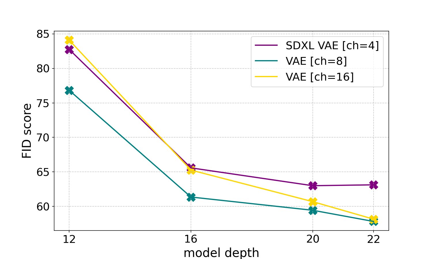
Figure 10: FID scores after training flow models with different sizes (parameterized via their depth) on the latent space of different autoencoders (4 latent channels, 8 channels and 16 channels) as discussed in Section 5.2.1. As expected, the flow model trained on the 16-channel autoencoder space needs more model capacity to achieve similar performance. At depth , the gap between 8-chn and 16-chn becomes negligible. We opt for the 16-chn model as we ultimately aim to scale to much larger model sizes.
图 10:在不同自编码器潜空间(4、8、16 潜通道)上、用不同规模(以深度参数化)的流模型训练后的 FID,见第 5.2.1 节。如预期,在 16 通道潜空间上训练的流模型需要更大容量才能达到相近表现。在深度 时,8 通道与 16 通道差距可忽略。我们最终选 16 通道模型,因目标是扩到大得多的规模。
Text Representation Similar to the encoding of images to latent representations, we also follow previous approaches (Saharia et al., 2022b; Balaji et al., 2022) and encode the text conditioning using pretrained, frozen text models. In particular, for all experiments, we use a combination of CLIP (Radford et al., 2021) models and a encoder-decoder text model. Specifically, we encode with the text encoders of both a CLIP L/14 model of Radford et al. (2021) as well as an OpenCLIP bigG/14 model of Cherti et al. (2023). We concatenate the pooled outputs, of sizes and respectively, to obtain a vector conditioning . We also concatenate the penultimate hidden representations channel-wise to a CLIP context conditioning . Next, we encode also to the final hidden representation, , of the encoder of a T5-v1.1-XXL model (Raffel et al., 2019). Finally, we zero-pad along the channel axis to dimensions to match the T5 representation and concatenate it along the sequence axis with to obtain the final context representation . These two caption representations, and , are used in two different ways as described in Section 4.
文本表示 与把图像编成潜表示类似,我们也沿用既有做法 (Saharia et al., 2022b; Balaji et al., 2022),用预训练、冻结的文本模型编码文本条件 。具体地,全部实验使用 CLIP (Radford et al., 2021) 与编码器–解码器文本模型的组合:用 Radford et al. (2021) 的 CLIP L/14 与 Cherti et al. (2023) 的 OpenCLIP bigG/14 的文本编码器分别编码 ,拼接尺寸为 与 的池化输出,得到向量条件 。我们也沿通道拼接倒数第二层隐表示,得到 CLIP 上下文条件 。接着把 编到 T5-v1.1-XXL (Raffel et al., 2019) 编码器的最终隐表示 。最后把 沿通道零填充到 维以匹配 T5,再沿序列维与 拼接,得到最终上下文表示 。这两种标题表示 与 按第 4 节所述以两种方式使用。
B.3 Preliminaries for the Experiments in Section 5.1.
B.3 第 5.1 节实验预备
Datasets We use two datasets to account for the missing of a standard text-to-image benchmark. As a widely used dataset, we convert the ImageNet dataset (Russakovsky et al., 2014) into a dataset suitable for text-to-image models by adding captions of the form “a photo of a ⟨class name⟩” to images, where ⟨class name⟩ is randomly chosen from one of the provided names for the image’s class label. As a more realistic text-to-image dataset, we use the CC12M dataset (Changpinyo et al., 2021) for training.
数据集 因缺少标准文生图基准,我们使用两个数据集。作为广泛使用的集合,我们把 ImageNet (Russakovsky et al., 2014) 转成适合文生图的形式:为图像添加形如「a photo of a ⟨class name⟩」的标题,其中 ⟨class name⟩ 从该图像类别标签的给定名称中随机选取。作为更贴近现实的文生图数据,训练使用 CC12M (Changpinyo et al., 2021)。
Optimization In this experiment, we train all models using a global batch size of 1024 using the AdamW optimizer (Loshchilov & Hutter, 2017) with a learning rate of and 1000 linear warmup steps. We use mixed-precision training and keep a copy of the model weights which gets updated every 100 training batches with an exponential moving average (EMA) using a decay factor of . For unconditional diffusion guidance (Ho & Salimans, 2022), we set the outputs of each of the three text encoders independently to zero with a probability of , such that we roughly train an unconditional model in of all steps.
优化 本实验中全部模型用全局 batch 1024、AdamW (Loshchilov & Hutter, 2017)、学习率 与 1000 步线性预热训练。使用混合精度,并保留一份每 100 个训练 batch 用衰减 的指数滑动平均(EMA)更新的权重副本。对无条件扩散引导 (Ho & Salimans, 2022),三个文本编码器输出各自以 概率置零,使大约 的步在训练无条件模型。
Evaluation As described in Section 5.1, we use CLIP scores, FID and validation losses to evaluate our models regularly during training on the COCO-2014 validation split (Lin et al., 2014).
评估 如第 5.1 节所述,我们在 COCO-2014 验证集 (Lin et al., 2014) 上定期用 CLIP 分数、FID 与验证损失评估模型。
As the loss values differ widely in magnitude and variance for different timesteps, we evaluate them in a stratified way on eight equally spaced values in the time interval .
因不同时间步损失的量级与方差差异很大,我们在时间区间 上取八个等距值分层评估。
To analyze how different approaches behave under different sampler settings, we produce 1000 samples for each of the samplers which differ in guidance scales as well as number of sampling steps. We evaluate these samples with CLIP scores using CLIP L/14 (Radford et al., 2021) and also compute FID between CLIP L/14 image features of these samples and the images of the validation set. For sampling, we always use a Euler discretization [26] of Equation 1 and six different settings: 50 steps with classifier-free-guidance scales 1.0, 2.5, 5.0, and 5, 10, 25 steps with classifier-free-guidance scale 5.0.
为分析不同做法在不同采样设定下的行为,我们对每种采样器(引导尺度与采样步数不同)各生成 1000 个样本。用 CLIP L/14 (Radford et al., 2021) 算 CLIP 分数,并在这些样本与验证集图像的 CLIP L/14 图像特征之间算 FID。采样始终用式 1 的 Euler 离散化 [26],六种设定:50 步、分类器无关引导尺度 1.0、2.5、5.0;以及 5、10、25 步、引导尺度 5.0。
B.4 Improving SNR Samplers for Rectified Flow Models
B.4 改进整流流的 SNR 采样器
As described in Section 2, we introduce novel densities for the timesteps that we use to train our rectified flow models. Figure 11 visualizes the distributions of the logit-normal sampler and the mode sampler introduced in Section 3.1. Notably, as we demonstrate in Section 5.1, the logit-normal sampler outperforms the classic uniform rectified flow formulation (Liu et al., 2022) and established diffusion baselines such as EDM (Karras et al., 2022) and LDM-Linear (Rombach et al., 2022).
如第 2 节所述,我们为训练整流流引入新的时间步密度 。图 11 可视化第 3.1 节引入的 logit-正态采样器 与 众数采样器。如第 5.1 节所示,logit-正态采样器 超过经典均匀整流流 (Liu et al., 2022) 以及 EDM (Karras et al., 2022)、LDM-Linear (Rombach et al., 2022) 等既有扩散基线。
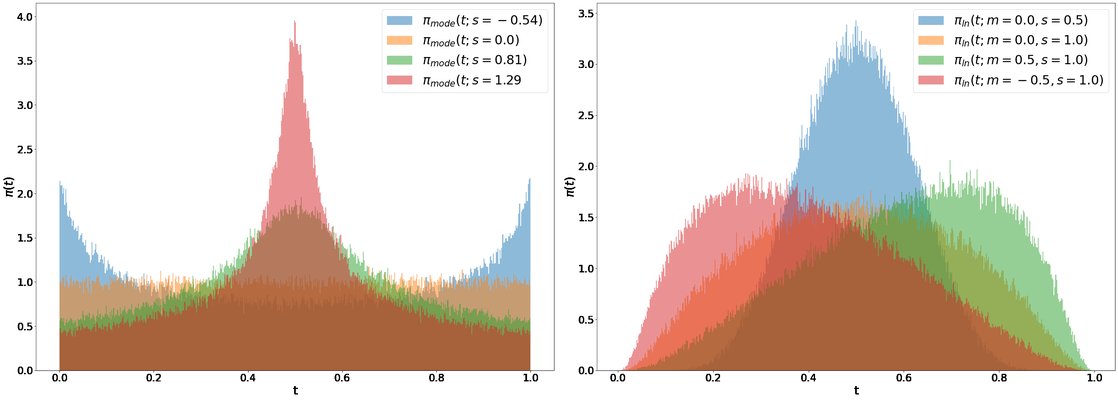
Figure 11: The mode (left) and logit-normal (right) distributions that we explore for biasing the sampling of training timesteps.
图 11:我们为偏置训练时间步采样所探索的众数(左)与 logit-正态(右)分布。
| “A raccoon wearing formal clothes, wearing a tophat and holding a cane. The raccoon is holding a garbage bag. Oil painting in the style of abstract cubism.” | “A bowl of soup that looks like a monster made out of plasticine” | “Two cups of coffee, one with latte art of a heart. The other has latte art of stars.” | “A smiling sloth is wearing a leather jacket, a cowboy hat, a kilt and a bowtie. The sloth is holding a quarterstaff and a big book. The sloth is standing on grass a few feet in front of a shiny VW van with flowers painted on it. wide-angle lens from below.” |
Figure 12: Qualitative effects of scaling. Displayed are examples demonstrating the impact of scaling training steps (left to right: 50k, 200k, 350k, 500k) and model sizes (top to bottom: depth=15, 30, 38) on PartiPrompts, highlighting the influence of training duration and model complexity.
| “A raccoon wearing formal clothes, wearing a tophat and holding a cane. The raccoon is holding a garbage bag. Oil painting in the style of abstract cubism.” | “A bowl of soup that looks like a monster made out of plasticine” | “Two cups of coffee, one with latte art of a heart. The other has latte art of stars.” | “A smiling sloth is wearing a leather jacket, a cowboy hat, a kilt and a bowtie. The sloth is holding a quarterstaff and a big book. The sloth is standing on grass a few feet in front of a shiny VW van with flowers painted on it. wide-angle lens from below.” |
图 12:缩放的定性效果。 展示在 PartiPrompts 上,训练步数(左到右:50k、200k、350k、500k)与模型规模(上到下:depth=15、30、38)对样本的影响,突出训练时长与模型复杂度的作用。
Appendix C Direct Preference Optimization
附录 C 直接偏好优化
| “a peaceful lakeside landscape with migrating herd of sauropods” | “a book with the words ‘Don’t Panic¡, written on it” | |
|---|---|---|
| 2B base | ||
| 2B w/ DPO | ||
| 8b base | ||
| 8b w/ DPO |
Figure 13: Comparison between base models and DPO-finetuned models. DPO-finetuning generally results in more aesthetically pleasing samples with better spelling.
| “a peaceful lakeside landscape with migrating herd of sauropods” | “a book with the words ‘Don’t Panic¡, written on it” | |
|---|---|---|
| 2B base | ||
| 2B w/ DPO | ||
| 8b base | ||
| 8b w/ DPO |
图 13:基座模型与经 DPO 微调模型的对比。DPO 微调通常带来更美观、拼写更好的样本。
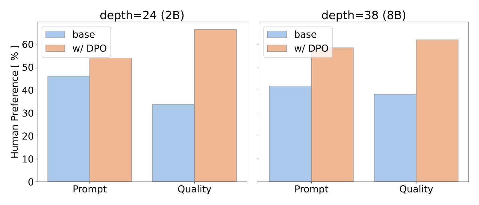
Figure 14: Human preference evaluation between base models and DPO-finetuned models. Human evaluators prefer DPO-finetuned models for both prompt following and general quality.
图 14:基座模型与经 DPO 微调模型的人类偏好评估。评分者在遵循提示与总体质量上均更偏好经 DPO 微调的模型。
Direct Preference Optimization (DPO) (Rafailov et al., 2023) is a technique to finetune LLMs with preference data. Recently, this method has been adapted to preference finetuning of text-to-image diffusion models (Wallace et al., 2023). In this section, we verify that our model is also amenable to preference optimization. In particular, we apply the method introduced in Wallace et al. (2023) to our 2B and 8B parameter base model. Rather than finetuning the entire model, we introduce learnable Low-Rank Adaptation (LoRA) matrices (of rank 128) for all linear layers as is common practice. We finetune these new parameters for 4k and 2k iteration for the 2B and 8B base model, respectively. We then evaluate the resulting model in a human preference study using a subset of 128 captions from the Partiprompts set (Yu et al., 2022) (roughly three voter per prompt and comparison). Figure 14 shows that our base models can be effectively tuned for human preference. Figure 13 shows samples of the respective base models and DPO-finetuned models.
直接偏好优化(DPO) (Rafailov et al., 2023) 是用偏好数据微调大语言模型的技术。近期已被改编用于文生图扩散模型的偏好微调 (Wallace et al., 2023)。本节验证我们的模型同样适合偏好优化。具体地,把 Wallace et al. (2023) 的方法用到我们的 2B 与 8B 基座模型上。我们不微调整网,而是按常见做法为全部线性层引入可学习的低秩适配(LoRA)矩阵(秩 128)。新参数分别对 2B 与 8B 基座微调 4k 与 2k 次迭代。随后在 Partiprompts (Yu et al., 2022) 的 128 条标题子集上做人偏好研究(每个提示与对比约三名评分者)。图 14 表明基座可被有效调向人类偏好;图 13 展示相应基座与经 DPO 微调模型的样本。
Appendix D Finetuning for instruction-based image editing
附录 D 面向指令式图像编辑的微调
A common approach for training instruction based image editing and general image-to-image diffusion models is to concatenate the latents of the input image to the noised latents of the diffusion target along the channel dimension before feeding the input into a U-Net (Brooks et al., 2023; Sheynin et al., 2023; Saharia et al., 2022a; Saharia et al., 2022c). We follow the same approach, concatenating input and target along the channels before patching, and demonstrate that the same method is applicable to our proposed architecture. We finetune the 2B parameter base model on a dataset consisting of image-to-image editing tasks similar to the distribution of the InstructPix2Pix dataset (Brooks et al., 2023) as well as inpainting, segmentation, colorization, deblurring and controlnet tasks similar to Emu Edit and Palette (Sheynin et al., 2023; Saharia et al., 2022a). As shown in Fig 15 we observe that the resulting 2B Edit model has the capability to manipulate text in a given image, even though no text manipulation tasks were included in the training data. We were not able to reproduce similar results when training a SDXL-based (Podell et al., 2023) editing model on the same data.
训练基于指令的图像编辑与一般图到图扩散模型的常见做法,是在送入 U-Net 前,把输入图像的潜表示与扩散目标的加噪潜表示沿通道拼接 (Brooks et al., 2023; Sheynin et al., 2023; Saharia et al., 2022a; Saharia et al., 2022c)。我们采用同一做法:在 patch 之前沿通道拼接输入与目标,并表明该方法同样适用于所提架构。我们在分布类似 InstructPix2Pix (Brooks et al., 2023) 的图到图编辑数据,以及类似 Emu Edit 与 Palette (Sheynin et al., 2023; Saharia et al., 2022a) 的补全、分割、上色、去模糊与 controlnet 任务上,微调 2B 基座。如图 15 所示,所得 2B Edit 模型具备在给定图像中操控文字的能力,尽管训练数据未包含文字操控任务。在同一数据上训练基于 SDXL (Podell et al., 2023) 的编辑模型时,我们未能复现类似结果。
| Input | Output 1 | Output 2 | |
|---|---|---|---|
| Write ”go small go home” instead | |||
| GO BIG OR GO UNET is written on the blackboard | |||
| change the word to UNOT | |||
| make the sign say MMDIT rules |
Figure 15: Zero Shot Text manipulation and insertion with the 2B Edit model
| 输入 | 输出 1 | 输出 2 | |
|---|---|---|---|
| Write ”go small go home” instead | |||
| GO BIG OR GO UNET is written on the blackboard | |||
| change the word to UNOT | |||
| make the sign say MMDIT rules |
图 15:2B Edit 模型的零样本文字操控与插入
Appendix E Data Preprocessing for Large-Scale Text-to-Image Training
附录 E 大规模文生图训练的数据预处理
E.1 Precomputing Image and Text Embeddings
E.1 预计算图像与文本嵌入
Our model uses the output of multiple pretrained, frozen networks as inputs (autoencoder latents and text encoder representations). Since these outputs are constant during training, we precompute them once for the entire dataset. This comes with two main advantages: (i) The encoders do not need to be available on the GPU during training, lowering the required memory. (ii) The forward encoding pass is skipped during training, saving time and total needed compute after the first epoch, see Tab. 7.
模型把多个预训练、冻结网络的输出(自编码器潜表示与文本编码器表示)当作输入。这些输出在训练中恒定,我们因而对整个数据集预计算一次。主要有两点好处:(i) 训练时 GPU 上不必加载编码器,降低显存;(ii) 跳过前向编码,在第一轮之后节省时间与总算力,见表 7。
| Model | Mem [GB] | FP [ms] | Storage [kB] | Delta [%] |
|---|---|---|---|---|
| VAE (Enc) | 0.14 | 2.45 | 65.5 | 13.8 |
| CLIP-L | 0.49 | 0.45 | 121.3 | 2.6 |
| CLIP-G | 2.78 | 2.77 | 202.2 | 15.6 |
| T5 | 19.05 | 17.46 | 630.7 | 98.3 |
Table 7: Key figures for preencoding frozen input networks. Mem is the memory required to load the model on the GPU. FP [ms] is the time per sample for the forward pass with per-device batch size of 32. Storage is the size to save a single sample. Delta [%] is how much longer a training step takes, when adding this into the loop for the 2B MMDiT-Model (568ms/it).
| 模型 | 显存 [GB] | 前向 [ms] | 存储 [kB] | 增量 [%] |
|---|---|---|---|---|
| VAE (Enc) | 0.14 | 2.45 | 65.5 | 13.8 |
| CLIP-L | 0.49 | 0.45 | 121.3 | 2.6 |
| CLIP-G | 2.78 | 2.77 | 202.2 | 15.6 |
| T5 | 19.05 | 17.46 | 630.7 | 98.3 |
表 7:冻结输入网络预编码的关键数字。 Mem 为把模型载入 GPU 所需显存。FP [ms] 为每设备 batch 32 时单样本前向时间。Storage 为保存单样本大小。Delta [%] 为把该项加入 2B MMDiT 训练循环后,单步相对变长多少(基线 568ms/it)。
This approach has two disadvantages: First, random augmentation for each sample every epoch is not possible and we use square-center cropping during precomputation of image latents. For finetuning our model at higher resolutions, we specify a number of aspect ratio buckets, and resize and crop to the closest bucket first and then precompute in that aspect ratio. Second, the dense output of the text encoders is particularly large, creating additional storage cost and longer loading times during training (c.f. Tab. 7). We save the embeddings of the language models in half precision, as we do not observe a deterioration in performance in practice.
该做法有两点代价:其一,每轮无法对样本做随机增强,预计算图像潜表示时我们用正方形中心裁剪。高分辨率微调时,我们指定若干宽高比桶,先缩放到最近桶再按该宽高比预计算。其二,文本编码器的稠密输出特别大,带来额外存储与更长加载时间(参见表 7)。我们把语言模型嵌入存成半精度,实践中未见表现明显变差。
E.2 Preventing Image Memorization
E.2 防止图像记忆
In the context of generative image models memorization of training samples can lead to a number of issues (Somepalli et al., 2023a; Carlini et al., 2023; Somepalli et al., 2023b). To avoid verbatim copies of images by our trained models, we carefully scan our training dataset for duplicated examples and remove them.
在生成图像模型中,记忆训练样本会带来若干问题 (Somepalli et al., 2023a; Carlini et al., 2023; Somepalli et al., 2023b)。为避免模型原样复制图像,我们仔细扫描训练数据中的重复样本并剔除。
Details on Deduplication
In accordance with the methods outlined by Carlini et al. (2023) and Somepalli et al. (2023a), we opt for SSCD (Pizzi et al., 2022) as the backbone for the deduplication process. The SSCD algorithm is a state-of-the-art technique for detecting near-duplicate images at scale, and it generates high-quality image embeddings that can be used for clustering and other downstream tasks. We also decided to follow Nichol (2022) to decide on a number of clusters . For our experiments, we use .
去重细节
依 Carlini et al. (2023) 与 Somepalli et al. (2023a) 的方法,我们选用 SSCD (Pizzi et al., 2022) 作为去重骨干。SSCD 是大规模近重复图像检测的先进技术,生成可用于聚类等下游任务的高质量图像嵌入。我们也依 Nichol (2022) 决定聚类数 ,实验中取 。
We utilize autofaiss (2023) for clustering. autofaiss (2023) is a library that simplifies the process of using Faiss (Facebook AI Similarity Search) for large-scale clustering tasks. Specifically, leverage FAISS index factory[^1] functionality to train a custom index with predefined number of centroids. This approach allows for efficient and accurate clustering of high-dimensional data, such as image embeddings.
聚类使用 autofaiss (2023)。该库简化了用 Faiss(Facebook AI Similarity Search)做大规模聚类的流程。具体地,我们利用 FAISS index factory 功能,用预定质心数训练定制索引,从而高效、准确地聚类图像嵌入等高维数据。
Algorithm 1 details our deduplication approach. We ran an experiment to see how much data is removed by different SSCD threshold as shown in Figure 16(b). Based on these results we selected four thresholds for the final run Figure 16(a).
算法 1 详述去重流程。我们实验了不同 SSCD 阈值去掉多少数据,见图 16(b)。据此为最终运行选取四个阈值,见图 16(a)。
E.3 Assessing the Efficacy of our Deduplication Efforts
E.3 评估去重效果
Carlini et al. (2023) devise a two-stage data extraction attack that generates images using standard approaches, and flags those that exceed certain membership inference scoring criteria. Carlini et al. (2023) bias their search towards duplicated training examples because these are orders of magnitude more likely to be memorized than non-duplicated examples (Somepalli et al., 2023a; Somepalli et al., 2023a; Lee et al., 2021).
Carlini et al. (2023) 设计两阶段数据提取攻击:用标准方式生成图像,再按成员推断打分准则标记可疑样本。他们偏向搜索重复训练样本,因为相对非重复样本,这些样本被记忆的概率高几个数量级 (Somepalli et al., 2023a; Lee et al., 2021)。
To assess how well our SSCD-based deduplication works, we follow Carlini et al. (2023) to extract memorized samples from small, specifically for this purpose trained models and compare them before and after deduplication. Two main step of the mentioned procedure include: 1) Generate many examples using the diffusion model in the standard sampling manner and with the known prompts. 2) Perform membership inference to separate the model’s novel generations from those generations which are memorized training examples. Algorithm 2 shows the steps to find the memorized samples based on Carlini et al. (2023). Note that we run this techniques two times; one for SD-2.1 model with only exact dedup removal as baseline, and for a model with the SD2.1 architecture but trained on removed exact duplication and near-duplication using SSCD (Pizzi et al., 2022).
为评估基于 SSCD 的去重效果,我们依 Carlini et al. (2023),从小的、专为此训练的模型中提取记忆样本,并比较去重前后。步骤主要包括:1)用已知提示、按标准采样生成大量样本;2)做成员推断,把模型的新颖生成与记忆自训练数据的生成分开。算法 2 给出基于 Carlini et al. (2023) 寻找记忆样本的步骤。我们运行两次:一次是仅做精确去重的 SD-2.1 作基线;一次是 SD2.1 架构、但在用 SSCD (Pizzi et al., 2022) 去掉精确与近重复后训练的模型。
We select the 350,000 most-duplicated examples from the training dataset based on SSCD (Pizzi et al., 2022) with threshold of 0.5, and generate 500 candidate images for each text prompt to increase the likelihood of finding memorization. The intuition is that for diffusion models, with high probability for two different random initial seeds ,. On the other hand, if under some distance measure d, it is likely that these generated samples are memorized examples. To compute the distance measure between two images, we use a modified Euclidean distance. In particular, we found that many generations were often spuriously similar according to distance (e.g., they all had gray backgrounds). We therefore instead divide each image into 16 non-overlapping 128 × 128 tiles and measure the maximum of the distance between any pair of image tiles between the two images. Figure 17 shows the comparison between number of memorized samples, before and after using SSCD with the threshold of 0.5 to remove near-duplicated samples. Carlini et al. (2023) mark images within clique size of 10 as memorized samples. Here we also explore different sizes for cliques. For all clique thresholds, SSCD is able to significantly reduce the number of memorized samples. Specifically, when the clique size is 10, trained SD models on the deduplicated training samples cut off at SSCD show a reduction in potentially memorized examples.
我们按 SSCD (Pizzi et al., 2022) 阈值 0.5 选出训练数据中重复最多的 35 万例,并对每个文本提示生成 500 张候选图以提高发现记忆的概率。直觉是:对扩散模型,不同随机初值 下,以高概率有 ;另一方面,若在某距离 下 ,则这些生成很可能是记忆样本。两图距离 我们用修改的欧氏 :许多生成按普通 会虚假相似(例如同为灰背景),因而把每张图划成 16 个不重叠的 块,取任意块对之间 的最大值。图 17 比较用阈值 0.5 的 SSCD 去掉近重复前后的记忆样本数。Carlini et al. (2023) 把团大小 10 内的图像标为记忆;我们也探索不同团大小。对全部团阈值,SSCD 都能显著减少记忆样本。特别地,团大小为 10 时,在 SSCD 截断的去重数据上训练的 SD 模型,潜在记忆样本约减少 。
0: – List of vectors in a single cluster, – List of item IDs corresponding to vecs, – FAISS index for similarity search within the cluster, – Threshold for determining duplicates Output: – Set of duplicate item IDs
1:
2: for to do
3: {Current vector}
4: {Current item ID}
5:
6: if then
7: continue
8: end if
9:
10:
11:
12:
13: for in do
14: if then
15:
16: end if
17: end for
18:
19: end for
20: Return {Final set of duplicate IDs}
Algorithm 1 Finding Duplicate Items in a Cluster
0: – 单簇内向量列表, – 对应 item ID 列表, – 簇内相似搜索的 FAISS 索引, – 判定重复的阈值 输出: – 重复 item ID 集合
1:
2: for to do
3: {当前向量}
4: {当前 item ID}
5:
6: if then
7: continue
8: end if
9:
10:
11:
12:
13: for in do
14: if then
15:
16: end if
17: end for
18:
19: end for
20: Return {最终重复 ID 集合}
算法 1 在簇内查找重复项
(a) Final result of SSCD deduplication over the entire dataset
(a) 在整个数据集上 SSCD 去重的最终结果
0: Set of prompts , Number of generations per prompt , Similarity threshold , Memorization threshold
0: Detection of memorized images in generated samples
1: Initialize to the set of most-duplicated examples
2: for each prompt do
3: for to do
4: Generate image with random seed
5: end for
6: end for
7: for each pair of generated images do
8: if distance then
9: Connect and in graph
10: end if
11: end for
12: for each node in do
13: Find largest clique containing the node
14: if size of clique then
15: Mark images in the clique as memorized
16: end if
17: end for
Algorithm 2 Detecting Memorization in Generated Images
0: 提示集合 ,每提示生成数 ,相似阈值 ,记忆阈值
0: 在生成样本中检测记忆图像
1: 将 初始化为重复最多的样本集合
2: for each prompt do
3: for to do
4: 用随机种子 生成图像
5: end for
6: end for
7: for each pair of generated images do
8: if distance then
9: 在图 中连接 与
10: end if
11: end for
12: for each node in do
13: 找包含该节点的最大团
14: if size of clique then
15: 将该团中的图像标为记忆
16: end if
17: end for
算法 2 检测生成图像中的记忆
Figure 17: SSCD-based deduplication prevents memorization. To assess how well our SSCD-based deduplication works, we extract memorized samples from small, specifically for this purpose trained models and compare them before and after deduplication. We plot a comparison between number of memorized samples, before and after using SSCD with the threshold of 0.5 to remove near-duplicated samples. Carlini et al. (2023) mark images within clique size of 10 as memorized samples. Here we also explore different sizes for cliques. For all clique thresholds, SSCD is able to significantly reduce the number of memorized samples. Specifically, when the clique size is 10, models on the deduplicated training samples cut off at SSCD show a reduction in potentially memorized examples.
图 17:基于 SSCD 的去重可抑制记忆。 为评估效果,我们从小的、专为此训练的模型中提取记忆样本,比较去重前后。图中对比用阈值 0.5 的 SSCD 去掉近重复前后的记忆样本数。Carlini et al. (2023) 把团大小 10 内的图像标为记忆;我们也探索不同团大小。对全部团阈值,SSCD 都能显著减少记忆样本。特别地,团大小为 10 时,在 SSCD 截断的去重数据上训练的模型,潜在记忆样本约减少 。