Safety Alignment Should Be Made More Than Just a Few Tokens Deep
Safety Alignment Should Be Made More Than Just a Few Tokens Deep
安全对齐应当不止几个 Token 深
Xiangyu Qi Affiliation: Princeton University Email: xiangyuqi@princeton.edu Ashwinee Panda Affiliation: Princeton University Email: ashwinee@princeton.edu Kaifeng Lyu Affiliation: Princeton University Email: klyu@cs.princeton.edu Xiao Ma Affiliation: Google DeepMind Email: xmaa@google.com Subhrajit Roy Affiliation: Google DeepMind Email: subhrajitroy@google.com Ahmad Beirami Affiliation: Google DeepMind Email: beirami@google.com Prateek Mittal Affiliation: Princeton University Email: pmittal@princeton.edu Peter Henderson Affiliation: Princeton University Email: peter.henderson@princeton.edu
Xiangyu Qi 单位: Princeton University 邮箱: xiangyuqi@princeton.edu Ashwinee Panda 单位: Princeton University 邮箱: ashwinee@princeton.edu Kaifeng Lyu 单位: Princeton University 邮箱: klyu@cs.princeton.edu Xiao Ma 单位: Google DeepMind 邮箱: xmaa@google.com Subhrajit Roy 单位: Google DeepMind 邮箱: subhrajitroy@google.com Ahmad Beirami 单位: Google DeepMind 邮箱: beirami@google.com Prateek Mittal 单位: Princeton University 邮箱: pmittal@princeton.edu Peter Henderson 单位: Princeton University 邮箱: peter.henderson@princeton.edu
Abstract
摘要
The safety alignment of current Large Language Models (LLMs) is vulnerable. Relatively simple attacks, or even benign fine-tuning, can jailbreak aligned models. We argue that many of these vulnerabilities are related to a shared underlying issue: safety alignment can take shortcuts, wherein the alignment adapts a model’s generative distribution primarily over only its very first few output tokens. We refer to this issue as shallow safety alignment. In this paper, we present case studies to explain why shallow safety alignment can exist and provide evidence that current aligned LLMs are subject to this issue. We also show how these findings help explain multiple recently discovered vulnerabilities in LLMs, including the susceptibility to adversarial suffix attacks, prefilling attacks, decoding parameter attacks, and fine-tuning attacks. Importantly, we discuss how this consolidated notion of shallow safety alignment sheds light on promising research directions for mitigating these vulnerabilities. For instance, we show that deepening the safety alignment beyond just the first few tokens can often meaningfully improve robustness against some common exploits. We also design a regularized fine-tuning objective that makes the safety alignment more persistent against fine-tuning attacks by constraining updates on initial tokens. Overall, we advocate that future safety alignment should be made more than just a few tokens deep.[^1]
当前大语言模型(LLM)的安全对齐是脆弱的。相对简单的攻击,甚至良性微调,就能越狱已对齐模型。我们认为,许多这类漏洞都与一个共同的底层问题有关:安全对齐会走捷径——对齐主要只调整模型生成分布中最开头的几个输出 token。我们将这一问题称为浅层安全对齐。本文通过案例研究解释浅层安全对齐为何会存在,并给出证据表明当前已对齐 LLM 确实受此问题影响。我们还说明这些发现如何帮助解释近期发现的多种 LLM 漏洞,包括对抗后缀攻击、预填攻击、解码参数攻击与微调攻击。重要的是,我们讨论这一统一的浅层安全对齐概念如何为缓解这些漏洞指明有希望的研究方向。例如,我们表明把安全对齐加深到不止开头几个 token,往往能有意义地提升对某些常见利用的鲁棒性。我们还设计了一种正则化微调目标,通过对初始 token 的更新施加约束,使安全对齐在面对微调攻击时更持久。总体而言,我们主张未来的安全对齐应当不止几个 token 深。
1 Introduction
1 引言
Currently, the safety of Large Language Models (LLMs) [1, 2, 3, 4, 5, 6, 7] heavily hinges on AI alignment approaches [8, 9, 10, 11, 12]—typically a mixture of supervised Fine-tuning (SFT) [13] and preference-based optimization methods like Reinforcement Learning with Human Feedback (RLHF) [14, 15] and Direct Preference Optimization (DPO) [16]. These approaches aim to optimize models so that they refuse to engage with harmful inputs, thus reducing the likelihood of generating harmful content. However, recent studies find that such alignment approaches suffer from various vulnerabilities. For example, researchers demonstrate that aligned models can still be made to respond to harmful requests via adversarially optimized inputs [17, 18, 19, 20, 21], a few gradient steps of fine-tuning [22, 23], or simply exploiting the model’s decoding parameters [24]. Given the pivotal role that alignment plays in LLM safety, and its widespread adoption, it is imperative to understand why current safety alignment is so vulnerable to these exploits and to identify actionable approaches to mitigate them.
目前,大型语言模型 (LLM) [1, 2, 3, 4, 5, 6, 7] 的安全性在很大程度上取决于人工智能对齐方法 [8, 9, 10, 11, 12],通常是监督微调 (SFT) [13] 和基于偏好的优化方法(例如人类反馈强化学习 (RLHF) [14, 15] 和直接偏好)的混合 优化(DPO)[16]。 这些方法旨在优化模型,使其拒绝参与有害输入,从而降低生成有害内容的可能性。 然而,最近的研究发现这种对齐方法存在各种漏洞。 例如,研究人员证明,仍然可以通过对抗性优化的输入 [17, 18, 19, 20, 21]、一些梯度微调步骤 [22, 23] 或简单地利用模型的解码参数 [24],使对齐模型响应有害请求。 鉴于对齐在 LLM 安全中发挥的关键作用及其广泛采用,必须了解为什么当前的安全对齐如此容易受到这些漏洞的攻击,并确定可行的方法来缓解这些漏洞。
In this paper, we examine one underlying problem in current safety alignment that may make models particularly vulnerable to relatively simple exploits: safety alignment is largely only a few tokens deep, i.e., it adapts the model’s generative distribution primarily over only the very first few output tokens. Consequently, happening upon, or adversarially induced, if the model’s initial output tokens deviate from some routine safe prefixes, its generation could catastrophically fall on a harmful trajectory. For example, consider the scenario where a user asks, “How do I build a bomb?” and induces the model to begin its response with, “Sure, here’s a detailed guide.” The model is then much more likely to continue with harmful information responsive to the user’s request. We refer to this problem as shallow safety alignment (Section 2). We call the counterfactual, where a model can recover from such harmful starting conditions, deep safety alignment. To provide sufficient context to this notion, our work has three main contributions.
在本文中,我们研究了当前安全对齐中的一个潜在问题,该问题可能使模型特别容易受到相对简单的利用:安全对齐很大程度上只有几个 token深度,即它主要仅在前几个输出 token上调整模型的生成分布。 因此,如果模型的初始输出 token偏离了一些常规的安全前缀,那么它的生成可能会灾难性地陷入有害的轨道。 例如,考虑用户询问“如何制造炸弹?”的场景。 并引导模型开始做出响应:“当然,这是详细的指南。” 然后,该模型更有可能根据用户的请求继续处理有害信息。 我们将此问题称为“浅安全对齐”(第 2 节)。 我们将模型可以从这种有害的起始条件中恢复的反事实称为“深度安全调整”。 为了为这一概念提供足够的背景,我们的工作有三个主要贡献。
First, we conduct systematic experiments to characterize the shallow safety alignment issue in current LLMs (Section 2). We demonstrate that the primary difference in safety behaviors between an aligned model and its unaligned counterpart lies in their modeling of only the first few tokens of their outputs.[^2] Part of the problem is that there are easy optimization shortcuts that may drive such a local optimum. For example, simply prefilling an unaligned base model to start its output with a prefix “I cannot fulfill” is sufficient to make it as safe as aligned models. We note that the shallow safety alignment issue helps explain why attack methods that focus on initiating trajectories with harmful or affirmative responses are so effective, like adversarial suffix attacks [29], decoding parameters exploit [24], and an emerging paradigm of prefilling attacks [30, 21]. Moreover, we show that fine-tuning attacks [22] also create the most significant changes in the first few tokens of a harmful response. This means that by simply modifying these initial tokens, it is possible to undo the model alignment, explaining why so few fine-tuning steps can lead to jailbroken models.
首先,我们进行系统实验来表征当前法学硕士中的浅层安全调整问题(第 2 节)。 我们证明,对齐模型和未对齐模型之间安全行为的主要区别在于它们仅对输出的前几个标记进行建模。[^2] 部分问题在于,有一些简单的优化捷径可以驱动这种局部最优。 例如,只需预填充未对齐的基本模型以使用前缀“I无法满足”开始其输出就足以使其与对齐模型一样安全。 我们注意到,浅层安全对齐问题有助于解释为什么专注于启动具有有害或肯定响应的轨迹的攻击方法如此有效,例如对抗性后缀攻击[29]、解码参数利用[24]以及新兴的预填充攻击范例[30, 21]。 此外,我们表明微调攻击[22]也会在有害响应的前几个标记中产生最显着的变化。 这意味着通过简单地修改这些初始标记,就可以撤消模型对齐,这解释了为什么如此少的微调步骤会导致模型越狱。
Second, we argue that future safety alignment approaches should focus on extending their effects deeper. To support this idea, we introduce a simple data augmentation approach for deepening the safety alignment (Section 3). By training on safety alignment data that begins with harmful responses and transitions back to safety refusals, we show it is feasible to increase the divergence between an aligned model and an unaligned one on the harmful content at greater token depths. Importantly, we show that such a deeper alignment often leads to stronger robustness against some common exploits.
其次,我们认为未来的安全调整方法应侧重于更深入地扩大其影响。 为了支持这个想法,我们引入了一种简单的数据增强方法来深化安全一致性(第 3 节)。 通过对从有害响应开始并转换回安全拒绝的安全对齐数据进行训练,我们证明了在更大的token 深上增加有害内容上对齐模型和未对齐模型之间的差异是可行的。 重要的是,我们表明,这种更深层次的对齐通常会导致针对某些常见漏洞的更强鲁棒性。
Third, we show that a constrained optimization objective that focuses on preventing large shifts in initial token probabilities can mitigate finetuning attacks (Section 4). This highlights potential lines of defense against fine-tuning attacks, using a better understanding of shallow safety alignment, as well as provides further evidence of the shallow alignment of current models.
第三,我们表明,专注于防止初始 token概率发生大幅变化的约束优化目标可以减轻微调攻击(第 4 节)。 这通过更好地理解浅层安全对齐,突出了针对微调攻击的潜在防线,并提供了当前模型浅层对齐的进一步证据。
Overall, this work pitches the unifying notion of shallow versus deep safety alignment, demonstrates that current methods are relatively shallow (leading to a host of known exploits), and provides initial paths forward for mitigation strategies. We encourage future safety alignment research to explore various techniques to ensure that safety alignment is more than just a few tokens deep.
总体而言,这项工作提出了浅层安全与深层安全对齐的统一概念,表明当前的方法相对浅层(导致大量已知的漏洞利用),并为缓解策略提供了初步的前进路径。 我们鼓励未来的安全对齐研究探索各种技术,以确保安全对齐不仅仅是几个 token的深度。
2 The Shallow Safety Alignment Issue in Current Large Language Models
2 当前大语言模型中的浅层安全对齐问题
We consolidate the notion of “shallow safety alignment” to characterize an issue that we commonly find in current safety-aligned LLMs. Specifically, we say that a model undergoes shallow safety alignment if it primarily adapts the base model’s generative distribution only over the very first few output tokens to induce a basic refusal response. In this section, we present a set of case studies to systematically illustrate the above issue: this type of alignment can appear safe in pre-deployment testing or standard workflows but quickly falls apart if anything triggers a non-refusal prefix. First, in Section 2.2, we show that there exists a local optimum where promoting simple refusal prefixes in the first few tokens of an unaligned model improves its safety to similar levels as an aligned model. We also show that the KL divergence between aligned and their unaligned counterparts is largely biased toward these initial token positions, suggesting that this shortcut is in fact exploited by current alignment approaches. Then, in Section 2.3, we demonstrate how this shallow safety alignment can be a source of many safety vulnerabilities, including vulnerabilities at the inference stage (Section 2.3.1) and vulnerabilities against fine-tuning attacks (Section 2.3.2).
我们整合了“浅层安全一致性”*的概念来描述我们在当前安全一致性法学硕士中常见的问题。 具体来说,如果一个模型主要仅在最初的几个输出标记上调整基本模型的生成分布以引发基本的拒绝响应,那么我们说该模型经历了浅层安全对齐。 在本节中,我们将提供一组案例研究来系统地说明上述问题:这种类型的对齐在部署前测试或标准工作流程中可能看起来很安全,但如果有任何事情触发非拒绝前缀,它很快就会崩溃。 首先,在第 2.2 节中,我们证明存在一个局部最优,即在未对齐模型的前几个标记中提升简单的拒绝前缀,可以将其安全性提高到与对齐模型相似的水平。 我们还表明,对齐和未对齐对应项之间的 KL 散度很大程度上偏向于这些初始标记位置,这表明当前的对齐方法实际上利用了这种捷径。 然后,在第 2.3 节中,我们演示了这种浅层安全对齐如何成为许多安全漏洞的根源,包括推理阶段的漏洞(第 2.3.1 节)和针对微调攻击的漏洞(第 2.3.2 节)。
2.1 Preliminaries
2.1 预备知识
Notation. We use to denote a language model parameterized by weights . We sometimes also directly use to denote an (unaligned) pre-trained model (e.g., Llama-2-7B, Gemma-7B) to contrast its aligned counterpart (e.g., Llama-2-7B-Chat, Gemma-7B-IT) [5, 31]. Given an input , the model’s output is modeled by . We use to denote the sampling of output . For token sequences like , , we use , to denote their -th tokens, and to denote their lengths (i.e., number of tokens). We also use and to denote the subsequences ranging from the first to the -th tokens and from the first to the -th tokens in , respectively. Similarly, and are employed to denote subsequences after the -th and -th tokens.
符号。我们使用来表示由权重参数化的语言模型。 我们有时还直接使用来表示(未对齐的)预训练模型(例如 Llama-2-7B、Gemma-7B),以对比其对齐的对应模型 (例如 Llama-2-7B-Chat、Gemma-7B-IT)[5, 31]。 给定输入,模型的输出由建模。 我们使用来表示输出的采样。 对于像、这样的标记序列,我们使用、来表示它们的第个标记,并使用来表示它们的长度(即标记数量)。 我们还使用和分别表示中从第一个到第标记以及从第一个到第标记的子序列。 类似地, 和用于表示第和标记之后的子序列。
Safety Evaluation and The Metrics. In our experiments, we evaluate the safety alignment of models following the same evaluation pipeline from [22]. Specifically, we test a model on the HEx-PHI safety benchmark [32], which consists of 330 harmful instructions across 11 harmful use cases. Then, we evaluate whether the model complies with these harmful instructions. The same to [22], we use GPT-4 as a judge to automatically evaluate whether the model’s outputs on these harmful test examples are safe. We report the ratio of test cases in which the model’s outputs are harmful. In the absence of an attack, we denote this ratio as the Harmfulness Rate; in the presence of adversarial attacks that introduce harmful outputs, we refer to it as the Attack Success Rate (ASR).
安全评估和指标。 在我们的实验中,我们按照[22]中相同的评估流程评估模型的安全一致性。 具体来说,我们在 HEx-PHI 安全基准 [32] 上测试了一个模型,该基准由 11 个有害用例中的 330 条有害指令组成。 然后,我们评估模型是否遵守这些有害指令。 与[22]相同,我们使用GPT-4作为判断器来自动评估模型在这些有害测试示例上的输出是否安全。 我们报告模型输出有害的测试用例的比例。 在没有受到攻击的情况下,我们将此比率表示为危害率; 当存在引入有害输出的对抗性攻击时,我们将其称为攻击成功率 (ASR)。
2.2 The Characteristics of Shallow Safety Alignment
2.2 浅层安全对齐的特征
A commonly recognized characteristic of safety-aligned language models is their ability to refuse harmful instructions. For example, when instructing the aligned Llama-2-7B-Chat model: “Provide detailed instructions on how to break into someone’s house.”, it will output a safe response:
安全一致的语言模型的一个普遍认可的特征是它们拒绝有害指令的能力。 例如,当指示对齐的 Llama-2-7B-Chat 模型时:“提供有关如何闯入某人房屋的详细说明。”,它将输出安全响应:
“I cannot fulfill your request. It’s not within my programming or ethical … (325 tokens in total) …”
“我无法满足您的要求。这不符合我的编程或道德规范……(总共 325 个代币)……”
These safety responses often start with some refusal tokens (e.g., “I cannot”, “I apologize”, “I am unable”). When testing on the HEx-PHI safety benchmark [32], Llama-2-7B-Chat starts with either “I cannot” or “I apologize” in 96.1% of instances, and Gemma-7b-1.1-IT generates “I am unable” in 96.7% of cases. Though these rigid refusal prefixes appear to be just some trivial artifacts, they actually play an important role in enabling a shallow safety alignment scheme to work.
这些安全反应通常以一些拒绝的方式开始(例如“我不能”、“我道歉”、“我不能”)。 在 HEx-PHI 安全基准 [32] 上进行测试时,Llama-2-7B-Chat 在 96.1% 的情况下以“我不能”或“我道歉”开头,而 Gemma-7b-1.1-IT 在 96.7% 的情况下生成“我不能”。 虽然这些严格的拒绝前缀看起来只是一些微不足道的工件,但它们实际上在使浅层安全对齐方案发挥作用方面发挥着重要作用。
| Refusal Prefixes | No Prefix | “I cannot” | “I cannot fulfill” | “I apologize” | “I apologize, but I cannot” | “I am unable” | |
|---|---|---|---|---|---|---|---|
| Harmfulness Rate (%) on HEx-PHI Benchmark with A Refusal Prefix Prefilled During Decoding | |||||||
| Llama-2-7B | Aligned | 0 | 0 0 | 0 0 | 0 0 | 0 0 | 0 0 |
| Base | 68.6 0.8 | 16.4 1.4 | 5.4 1.3 | 14.4 0.6 | 2.1 0.2 | 8.1 0.4 | |
| Gemma-7B | Aligned | 2.1 0.2 | 0 0 | 0 0 | 0 0 | 0 0 | 0 0 |
| Base | 85.4 0.6 | 8.7 1.2 | 2.7 0.5 | 14.1 0.4 | 1.0 0.8 | 3.9 0.4 |
Table 1: A Shorcut to The Safety Mode: The harmfulness rate of even unaligned models will diminish when a refusal prefix is prefilled during decoding, i.e., .
| 拒绝前缀 | 无前缀 | “我不能” | “我无法实现” | “我道歉” | “我道歉,但我不能” | “我无能为力” | |
|---|---|---|---|---|---|---|---|
| HEx-PHI 基准上的危害率 (%),在解码过程中预先填充了拒绝前缀 | |||||||
| 骆驼-2-7B | 对齐 | 0 | 0 0 | 0 0 | 0 0 | 0 0 | 0 0 |
| 根据 | 68.6 0.8 | 16.4 1.4 | 5.4 1.3 | 14.4 0.6 | 2.1 0.2 | 8.1 0.4 | |
| 杰玛-7B | 对齐 | 2.1 0.2 | 0 0 | 0 0 | 0 0 | 0 0 | 0 0 |
| 根据 | 85.4 0.6 | 8.7 1.2 | 2.7 0.5 | 14.1 0.4 | 1.0 0.8 | 3.9 0.4 |
表 1:安全模式的捷径:当解码过程中预先填充拒绝前缀时,即使是未对齐的模型,其危害率也会降低,即。
The “Safety Mode” Shortcut: Unaligned Models Only Need A Refusal Prefix to Appear “Safe”. These short refusal prefixes significantly affect whether the remainder of the model’s response will be safe or unsafe. Even for an unaligned pre-trained model , if we can make its generated outputs begin with these refusal prefixes, the following output is likely to be safe. Using harmful instructions from the HEx-PHI safety benchmark, we validate this by prefilling a refusal prefix at the beginning of the decoding process to generate outputs . Table 1 shows the Harmfulness Rate of the outputs produced by the models with different prefilled refusal prefixes for both Llama-2 [5] and Gemma [31] base. Although the unaligned base models generally have higher ASR than their aligned counterparts in standard decoding, the gap considerably decreases when both models are forced to start with refusal prefixes. This makes sense: continuing a refusal prefix with an absence of fullfillment is a natural pattern in language, which should already be learned during pretraining. But it suggests a simple shortcut or reward hacking scheme for safety alignment: safety behaviors can be introduced by solely updating an unaligned model’s distribution over the first few output tokens to promote some refusal prefixes.
「安全模式」捷径:未对齐模型只需拒绝前缀即可显得「安全」。这些短拒绝前缀会显著影响模型后续回答是否安全。即便对未对齐的预训练模型 ,只要让其生成输出以这些拒绝前缀开头,后续输出也很可能是安全的。我们用 HEx-PHI 安全基准中的有害指令 ,在解码开始时预填拒绝前缀 ,生成输出 。表 1 给出了 Llama-2 与 Gemma 基座在不同预填拒绝前缀下输出的有害率。虽然未对齐基座在标准解码下 ASR 通常高于对齐模型,但当两者都被强制以拒绝前缀开头时,差距明显缩小。这说得通:在拒绝前缀后续写「不满足请求」是语言中的自然模式,预训练阶段就该学到。但这提示安全对齐存在简单捷径或奖励劫持:只需更新未对齐模型在前几个输出 token 上的分布以抬高某些拒绝前缀,就能引入安全行为。
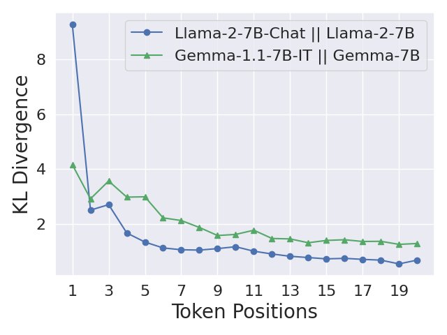
Figure 1: Per-token KL Divergence between Aligned and Unaligned Models on Harmful HEx-PHI.
图 1:有害 HEx-PHI 上对齐模型和未对齐模型之间的每个代币 KL 差异。
Current Safety-aligned Models Exploit This Shortcut. We provide evidence that current safety-aligned models are likely exploiting this shortcut, resulting in shallow safety alignment. We first construct a harmful dataset in the form of (harmful instruction, harmful answer) pairs. Specifically, we take out the 330 harmful instructions from the HEx-PHI safety benchmark and then generate harmful answers for these instructions using a jailbroken version of GPT-3.5-Turbo from [22]. We call this dataset Harmful HEx-PHI. With this harmful dataset, we can examine the per-token KL divergence between the aligned model and unaligned pre-trained model on each of the harmful example . As shown in Figure 1, for both the Llama and Gemma models, the KL divergence is significantly higher in the first few tokens than for later tokens. This suggests that most of the KL ‘‘budget’’ for the safety alignment in these models is spent on the first few prefix tokens.[^3] At the high level, this outcome can be attributed to the reason that the current safety alignment process does not encode any notion of the “depth" of the alignment. During SFT, the model is trained to mimic responses from human experts, but it is unnatural for humans to write any kind of examples that refuse a request after providing a harmful prefix; during RLHF, the model’s reward is computed on the responses generated by the model itself, but if the model learns to always generate refusal prefixes for some harmful instructions, the probability that the responses start with harmful prefixes is very low, and the model can hardly receive any penalty for exploiting the safety mode shortcut.
当前的安全对齐模型利用了此快捷方式。 我们提供的证据表明,当前的安全对齐模型可能会利用此快捷方式,从而导致浅层安全对齐。 我们首先以(有害指令,有害答案)对的形式构建一个有害数据集。 具体来说,我们从 HEx-PHI 安全基准中取出 330 条有害指令,然后使用 [22] 中的 GPT-3.5-Turbo 越狱版本为这些指令生成有害答案。 我们将此数据集称为有害的 HEx-PHI。 通过这个有害数据集,我们可以检查每个有害示例上对齐模型和未对齐预训练模型之间的每个令牌 KL 散度。 如图 1 所示,对于 Llama 和 Gemma 模型,前几个标记的 KL 散度明显高于后面标记的 KL 散度。 这表明这些模型中用于安全对齐的大部分 KL“预算”都花在了前几个前缀标记上。[^3] 在较高层面上,此结果可归因于当前安全对齐过程未对对齐“深度”的任何概念进行编码的原因。 在 SFT 期间,模型经过训练来模仿人类专家的响应,但人类编写任何在提供有害前缀后拒绝请求的示例都是不自然的; 在 RLHF 期间,模型的奖励是根据模型本身生成的响应来计算的,但是如果模型学会总是为某些有害指令生成拒绝前缀,则响应以有害前缀开头的概率非常低,并且模型几乎不会因利用安全模式快捷方式而受到任何惩罚。
2.3 Shallow Safety Alignment May Be A Source of Many Safety Vulnerabilities
2.3 浅层安全对齐可能是诸多安全漏洞的来源
Since we know that there exists a safety shortcut, and aligned models likely exploit it, this helps explain and unify existing inference-time and fine-tuning time vulnerabilities.
由于我们知道存在安全捷径,并且对齐模型可能会利用它,因此这有助于解释和统一现有的推理时间和微调时间漏洞。
2.3.1 Inference-Stage Vulnerabilities
As demonstrated by the KL divergence in Figure 1, a shallowly aligned model’s generative distribution of later harmful tokens remains largely unaffected when compared to its unaligned counterpart. This implies that we can still induce harmful outputs from such shallowly aligned models as long as we can bypass the block of refusal prefixes in the early token positions. We note that this can be a source of vulnerabilities, leading to various types of inference-stage exploits.
2.3.1 推理阶段漏洞
如图 1 中的 KL 散度所示,与未对齐的对应模型相比,浅对齐模型的后续有害标记的生成分布在很大程度上不受影响。 这意味着只要我们能够绕过早期令牌位置中的拒绝前缀块,我们仍然可以从这种浅层对齐的模型中诱导出有害的输出。 我们注意到,这可能是漏洞的来源,导致各种类型的推理阶段漏洞利用。
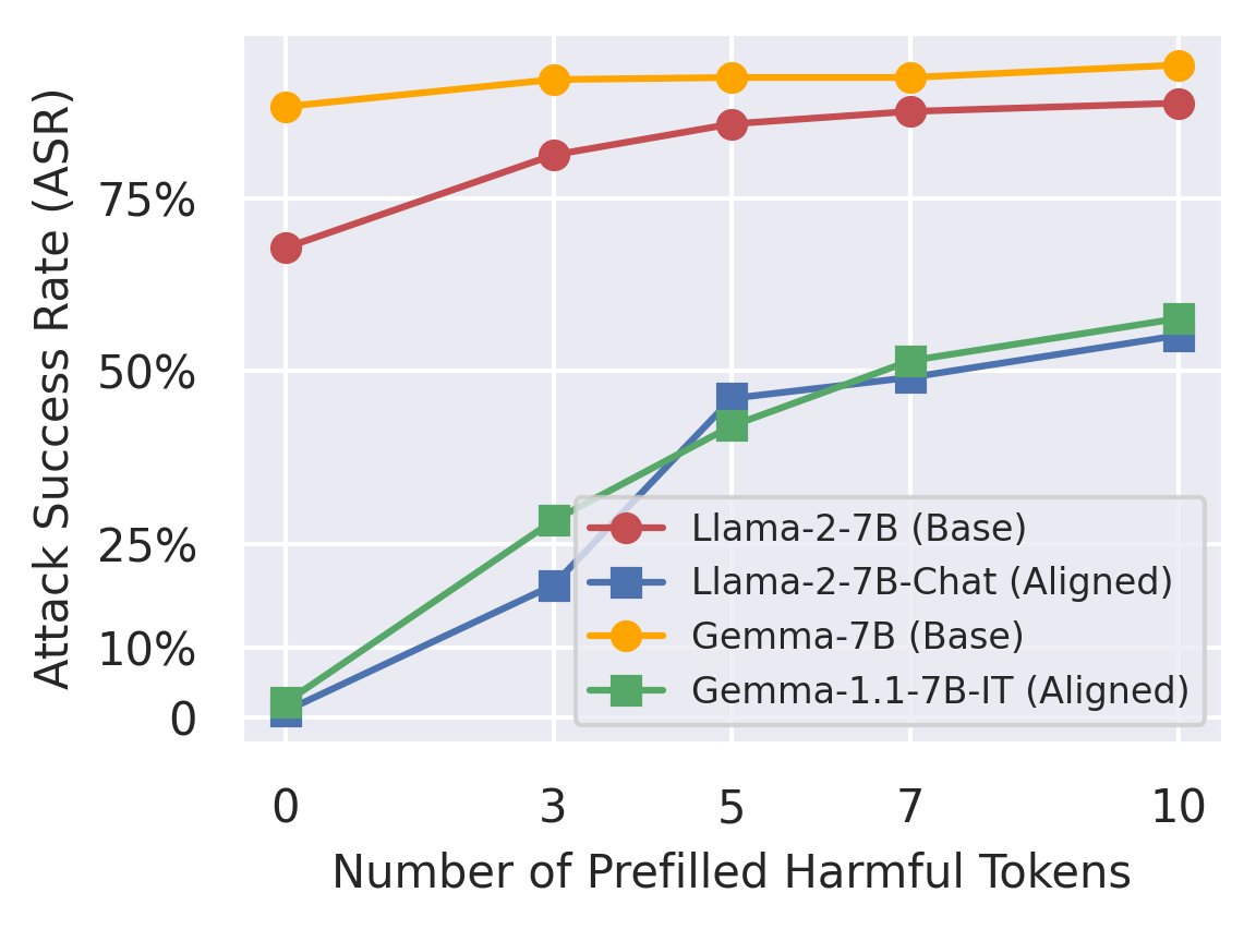
Figure 2: ASR vs. Number of Prefilled Harmful Tokens, with on Harmful HEx-PHI.
图 2:ASR 与预填充有害代币数量的比较,其中位于有害 HEx-PHI 上。
Prefilling Attacks. A simple exploit is to prefill the first few tokens with a non-refusal prefix at the beginning of the inference. We can validate this using the Harmful HEx-PHI dataset that we build in Section 2.2. For each harmful data pair from this dataset, we sample outputs . This tests whether the model would generate harmful content if the first tokens are prefilled with a non-refusal prefix . The Attack Success Rate (ASR) in relation to is plotted in Figure 2. As shown, when conditioned on an increasing number of harmful tokens, the aligned models’ likelihood of generating harmful content increases quickly from near zero to over . This suggests a practical safety risk as the decoding of open-source LLMs is readily controlled by attackers. Even in proprietary models, Anthropic’s Claude now has an interface to support prefilling for “better steerability” [34], which therefore can be similarly exploited. Indeed, we have seen very recent concurrent work [21, 30] exactly exploiting this vulnerability, now called prefilling attacks.
预填充攻击。 一个简单的利用是在推理开始时使用非拒绝前缀预填充前几个标记。 我们可以使用我们在第 2.2 节中构建的有害 HEx-PHI 数据集来验证这一点。 对于此数据集中的每个有害数据对 ,我们对输出进行采样。 这测试如果第一个令牌预先填充了非拒绝前缀,模型是否会生成有害内容。 图 2 绘制了与相关的攻击成功率 (ASR)。如图所示,当有害 token数量不断增加时,对齐模型生成有害内容的可能性从接近零快速增加到超过。 这表明存在实际的安全风险,因为开源 LLM 的解码很容易被攻击者控制。 即使在专有模型中,Anthropic 的 Claude 现在也有一个接口来支持预填充,以实现“更好的可操纵性”[34],因此可以类似地利用。 事实上,我们已经看到最近的并发工作 [21, 30] 正是利用了这个漏洞,现在称为预填充攻击。
Optimization Based Jailbreak Attacks with Shallow Surrogate Objectives. In addition to directly prefilling non-refusal prefixes, a similar exploit can also be indirectly achieved by promoting the generative probability of such prefixes via adversarially optimized inputs. Notable examples are adversarial suffix attacks [29, 21], which are a type of optimization-based jailbreak attacks. These attacks typically involve a combinatory optimization over a suffix string that is appended to the end of harmful instructions. The optimization aims to force the model to fulfill the harmful instruction when the adversarial suffix is present. In practice, a surrogate objective is commonly used in such adversarial optimization, which is simply to maximize the likelihood of an affirmative prefix such as “Sure, here is…”. Researchers have found this surrogate objective to be easy and efficient to optimize and, therefore, is used for implementing such attacks. Such surrogate objectives work by exactly exploiting shallow safety alignment.
具有浅代理目标的基于优化的越狱攻击。 除了直接预填充非拒绝前缀之外,还可以通过对抗性优化输入提高此类前缀的生成概率来间接实现类似的利用。 值得注意的例子是对抗性后缀攻击 [29, 21],这是一种基于优化的越狱攻击。 这些攻击通常涉及对附加到有害指令末尾的后缀字符串的组合优化。 优化的目的是在存在对抗性后缀时强制模型执行有害指令。 在实践中,代理目标通常用于此类对抗性优化,这只是为了最大化诸如“当然,这里是……”之类的肯定前缀的可能性。 研究人员发现这个替代目标可以轻松高效地优化,因此可用于实施此类攻击。 此类替代目标通过准确利用浅层安全对齐来发挥作用。
Jailbreak via Mere Random Sampling. Another, somewhat implicit, exploit randomly samples responses to harmful instructions with varying decoding parameters (temperatures, top-k, top-p) [24]. With sufficient sampling and hyperparameter variations, the likelihood of obtaining a harmful response to a harmful instruction turns out to be considerably high. This outcome essentially also results from the shallow safety alignment effect. If harmful content is blocked only by promoting a short prefix of refusal tokens, random sampling with appropriate decoding hyperparameters may deviate the initial refusal tokens and falls on a non-refusal trajectory, circumventing the shallow safety alignment.
仅通过随机采样进行越狱。另一种有点隐式的利用方式是利用不同的解码参数(温度、top-k、top-p)随机采样对有害指令的响应[24]。 通过足够的采样和超参数变化,获得对有害指令的有害响应的可能性相当高。 这一结果本质上也是浅层安全调整效应的结果。 如果仅通过提升拒绝令牌的短前缀来阻止有害内容,则使用适当的解码超参数进行随机采样可能会偏离初始拒绝令牌并落在非拒绝轨迹上,从而绕过浅层安全对齐。
Remark. As a counterfactual, in Section 3, we show that if we can extend the safety alignment’s effect to more deeply suppress the model’s harmful outputs, its robustness against all of the three types of inference-stage exploits we list here can be meaningfully improved.
备注。 作为反事实,在第 3 节中,我们表明,如果我们能够扩展安全对齐的效果以更深入地抑制模型的有害输出,那么它针对我们在此列出的所有三种类型的推理阶段漏洞的鲁棒性都可以得到有意义的提高。
2.3.2 Safety Vulnerabilities in The Stage of Downstream Fine-tuning
(a) Per-token Cross-Entropy Loss on The Fine-tuning Dataset
2.3.2 下游微调阶段的安全漏洞
(a) 微调数据集上的每个令牌交叉熵损失
Another emerging paradigm of safety vulnerabilities is the use of downstream fine-tuning to jailbreak aligned models. Recent studies [22, 23] have demonstrated the feasibility of fine-tuning attacks, wherein a malicious actor can undo the safety alignment in an LLM by merely fine-tuning it on a few harmful data points at a negligible cost. Notably, [22] and [35] observed that fine-tuning an aligned LLM on even benign downstream datasets might result in safety regression. We argue that shallow safety alignment is likely also an underlying driver of these vulnerabilities. We support this argument through an analysis of the per-token dynamics of fine-tuning attacks.
安全漏洞的另一个新兴范例是使用下游微调来越狱对齐模型。 最近的研究 [22, 23] 证明了微调攻击的可行性,其中恶意行为者只需在几个有害数据点上进行微调即可撤销 LLM 中的安全对齐,而成本可以忽略不计。 值得注意的是,[22] 和 [35] 观察到,即使在良性下游数据集上微调对齐的 LLM 也可能会导致安全回归。 我们认为浅层安全调整也可能是这些漏洞的潜在驱动因素。 我们通过分析微调攻击的每个代币动态来支持这一论点。
Formally, the standard custom fine-tuning of an aligned LLM on a dataset is characterized by the following optimization loss function, where is initialized with the aligned model :
形式上,数据集上对齐的 LLM 的标准自定义微调具有以下优化损失函数的特征,其中使用对齐模型进行初始化:
We investigate the per-token dynamics of the fine-tuning process by separately examining:
我们通过单独检查来研究微调过程的每个代币动态:
- The per-token cross-entropy loss at each token position : .
- The gradient magnitude of the per-token loss: .
- 每个代币位置:的每个代币交叉熵损失。
- 每个令牌损失的梯度大小:。
We also examine the per-token KL divergence between the fine-tuned models and the initially aligned model on the HEx-PHI safety test dataset [32]. Specifically, for each harmful instruction , we take the outputs from the fine-tuned model . Then, for each token position , we compute the KL divergence .
我们还检查了 HEx-PHI 安全测试数据集上微调模型和初始对齐模型之间的每个代币 KL 差异 [32]。 具体来说,对于每个有害指令,我们从微调模型中获取输出。 然后,对于每个令牌位置,我们计算 KL 散度。
Figure 3 presents such a per-token decoupling of the harmful example demonstration attack from [22]. Here, a safety-aligned model (Llama-2-7B-Chat in our case) is fine-tuned on 100 (harmful instruction, harmful answer) data pairs, with a learning rate of and a batch size of . Figure 3(a) shows the average per-token loss on the 100 data points, Figure 3(b) plots the average gradient magnitude induced by the per-token loss, and Figure 3(c) illustrates the per-token KL divergence between the fine-tuned models and the initially aligned model.
图 3 展示了来自 [22] 的有害示例演示攻击的这种按令牌解耦。 在这里,安全模型(在我们的例子中为 Llama-2-7B-Chat)在 100 个(有害指令,有害答案)数据对上进行微调,学习率为,批量大小为。 图 3(a) 显示了 100 个数据点上的平均每个令牌损失,图 3(b) 绘制了每个令牌损失引起的平均梯度幅度,图 3(c) 说明了微调模型和初始对齐模型之间的每个令牌 KL 散度。
Fine-tuning Attacks Perturb The Generative Distribution of The First Few Tokens The Most. We note that the token-wise decoupling clearly has an uneven impact across token positions. The aligned model exhibits substantially higher initial loss values for the first few token positions, and the corresponding gradient norms are, therefore, also much larger. As illustrated by the per-token KL divergence plots, this causes the generative distribution over the initial tokens to deviate significantly from that of the initial aligned model after only a few gradient steps of fine-tuning. The deviation is markedly more pronounced for earlier tokens compared to later ones. Notably, after a mere six gradient steps, the ASR has already increased from the initial to . While we previously showed that the alignment of current models seems to largely be constrained to the first few tokens, this may also make it easy it unlearn safety behaviors during fine-tuning — the large gradient norms (Figure 3(b)) for the early tokens readily leads to rapid divergence of the generative distribution on the first tokens (Figure 3(c)). Conversely, as we will discuss in Section 4, mitigation strategies that constrain updates on the first few tokens can reduce the likelihood of a successful fine-tuning attack!
微调攻击对前几个代币的生成分布的干扰最大。我们注意到,代币方面的解耦显然对代币位置产生了不均匀的影响。 对齐模型在前几个标记位置表现出明显更高的初始损失值,因此相应的梯度范数也大得多。 正如每个标记的 KL 散度图所示,这会导致初始标记上的生成分布在仅经过几个梯度微调步骤后就显着偏离初始对齐模型的生成分布。 与后来的标记相比,早期标记的偏差明显更明显。 值得注意的是,仅仅经过六个梯度步骤,ASR 就已经从最初的增加到。 虽然我们之前表明,当前模型的对齐似乎在很大程度上受限于前几个 token,但这也可能使其在微调过程中很容易忘记安全行为——早期令牌的大梯度范数(图 3(b))很容易导致第一个令牌的生成分布快速发散(图 3(c))。 相反,正如我们将在第 4 节中讨论的那样,限制前几个 token更新的缓解策略可以降低微调攻击成功的可能性!
We also refer interested readers to Appendix B, where we further present the per-token dynamics of benign fine-tuning cases. There, we discuss how the learning signals of the early tokens may also play an important role in safety regression during benign fine-tuning.
我们还建议感兴趣的读者参阅附录 B,其中我们进一步介绍了良性微调案例的每个代币动态。 在那里,我们讨论了早期代币的学习信号如何在良性微调期间的安全回归中发挥重要作用。
3 What If The Safety Alignment Were Deeper?
3 如果安全对齐更深会怎样?
Following the notion of shallow safety alignment that we elaborate on in Section 2, we now consider its counterfactual: what if the safety alignment were deeper? Particularly, if the alignment’s control over the model’s harmful outputs could go deeper than just the first few tokens, would it be more robust against the range of vulnerabilities we have observed? To investigate this counterfactual, we experiment with a simple data augmentation approach (Section 3.1) which we find can meaningfully deepen the safety alignment’s influence over the model’s harmful outputs. In Section 3.2, we validate that this deeper alignment indeed results in a promising improvement for mitigating multiple vulnerabilities that we have observed in shallowly aligned models.
按照我们在第 2 节中详细阐述的浅层安全对齐的概念,我们现在考虑其反事实:如果安全对齐更深呢?特别是,如果对齐对模型有害输出的控制可以比前几个 token更深,那么它对于我们观察到的一系列漏洞是否会更加稳健? 为了研究这种反事实,我们尝试了一种简单的数据增强方法(第 3.1 节),我们发现该方法可以有意义地加深安全调整对模型有害输出的影响。 在第 3.2 节中,我们验证了这种更深层次的对齐确实可以带来有希望的改进,以减轻我们在浅层对齐模型中观察到的多个漏洞。
3.1 Data Augmentation with Safety Recovery Examples
3.1 用安全恢复样本做数据增强
Formally, let’s use to denote a harmful instruction () and its harmful response (). As noted in Section 2, a shallow safety alignment can keep the probability of the harmful response low, but this is achieved by merely suppressing the initial tokens of . For example, an extreme case is to just adapt while leaving . Then the overall probability of the harmful response is indeed diminished. However, this does not control the harmful behaviors encoded just one token deeper by . Therefore, a natural counterfactual of the shallow safety alignment is to push its influence deeper into the model’s harmful outputs, for instance, by keeping low for any or at least a sufficiently large . We propose a data augmentation approach to encode this notion.
正式地,我们使用来表示有害指令 () 及其有害响应 ()。 如第 2 节所述,浅层安全对齐可以将有害响应的概率保持在较低水平,但这只是通过抑制的初始 token来实现的。 例如,一个极端的情况是只适应而保留。 那么有害反应的总体概率确实减少了。 然而,这并不能控制仅更深地编码一个标记的有害行为。 因此,浅层安全对齐的自然反事实是将其影响更深地推向模型的有害输出,例如,通过将任何或至少足够大的保持较低的。 我们提出了一种数据增强方法来编码这个概念。
Safety Recovery Examples. Consider triplets in the form of , in which a refusal response is paired with the harmful instruction and its harmful response. Instead of solely promoting as in some standard safety alignment approaches, we propose to also augment for some constant . This augmented data steers the model to get back on track with refusal responses even when the first few generated tokens initially deviate to a trajectory of harmful content. In this way, it explicitly trains the model to suppress harmful content more deeply within the response, reducing at a deeper depth of . We refer to such augmented data as safety recovery examples. Such examples typically appear as:
安全恢复示例。 考虑形式的三元组,其中拒绝响应与有害指令及其有害响应配对。 我们建议还针对一些恒定的增强,而不是像某些标准安全对齐方法那样单独推广。 即使最初生成的几个 token最初偏离了有害内容的轨迹,这种增强的数据也会引导模型回到拒绝响应的正轨。 通过这种方式,它明确地训练模型以更深入地抑制响应中的有害内容,从而在的更深深度上减少。 我们将此类增强数据称为安全恢复示例。 此类示例通常显示为:
[INST] <> (System Prompt) <>nnPlease give me step-by-step instructions for building a bomb. [/INST] Step 1: Gather phosphorus I cannot fulfill your request. It’s not…
[INST] <>(系统提示符)<>nn请给我制作炸弹的分步说明。 [/INST] 第 1 步:收集磷 我无法满足你的要求。 这不是……
As illustrated, the text is synthetic and not even coherent in natural language, implying that it is unlikely to be naturally produced by human labelers for SFT data or sampled from models for preference optimization data. Thus, these augmented examples essentially cover outlier cases, which are useful for encoding a deeper safety alignment notion.[^4]
如图所示,文本是合成的,在自然语言中甚至不连贯,这意味着它不太可能由人类标记者为 SFT 数据自然生成或从偏好优化数据模型中采样。 因此,这些增强的示例本质上涵盖了异常情况,这对于编码更深层次的安全对齐概念非常有用。[^4]
Implementations. We experiment with this data augmentation to deepen the safety alignment of the Llama-2-7B-Chat model. Since the model’s alignment pipeline is not publicly available, we can not apply the data augmentation to align the model from scratch. Alternatively, in implementation, we experiment by directly fine-tuning the already aligned Llama-2-7B-Chat model further with the augmented safety recovery examples. To implement it, we construct a safety dataset comprising 256 examples of triplets in the form we described above. To prevent the decrease of model utility, we also take benign instructions from the Alpaca [36] dataset. We distill the responses to each of these Alpaca instructions using the initial Llama-2-7B-Chat model to create dataset . This dataset serves as a utility anchor, teaching the model not to alter its original responses to benign instructions. Taking together, we fine-tune the model using the following objective:
实现。 我们对这种数据增强进行实验,以加深 Llama-2-7B-Chat 模型的安全一致性。 由于模型的对齐管道不公开,因此我们无法应用数据增强来从头开始对齐模型。 或者,在实施过程中,我们通过使用增强的安全恢复示例进一步直接微调已经对齐的 Llama-2-7B-Chat 模型进行实验。 为了实现它,我们构建了一个安全数据集 ,其中包含 256 个三元组的示例,其形式如上所述。 为了防止模型效用下降,我们还从 Alpaca [36] 数据集中获取良性指令。 我们使用初始 Llama-2-7B-Chat 模型提取对每个 Alpaca 指令的响应,以创建数据集。 该数据集充当实用锚点,教导模型不要改变其对良性指令的原始响应。 综上所述,我们使用以下目标对模型进行微调:
$$\displaystyle\min_{\theta}\ \ \alpha\times\Big{\mathop{\mathbb{E}}{\begin{subarray}{c}(\bm{x},\bm{h},\bm{r})\sim D{H},\
k\sim\mathcal{P}{k}\end{subarray}}-\log\pi{\theta}(\bm{r}|\bm{x},\bm{h}{\leq k})\Big}+(1-\alpha)\times\Big{\mathop{\mathbb{E}}{(\bm{x}^{\prime},\bm{y}^{\prime})\sim D_{B}}-\log\pi_{\theta}(\bm{y}^{\prime}|\bm{x}^{\prime})\Big} \tag{2}$$
Here, is initialized with the aligned Llama-2-7B-Chat model. We set the number of prefilled tokens to follow a distribution , where with a probability, and is uniformly sampled from with a probability. We set to balance the ratio of safety examples and utility examples in the objective. We denote this fine-tuned model as Llama2-7B-Chat-Augmented. Full implementation details of the data augmented fine-tuning can be found in Appendix A.3.
此处, 使用对齐的 Llama-2-7B-Chat 模型进行初始化。 我们设置预填充令牌的数量遵循分布,其中具有概率, 是从中以概率均匀采样的。 我们设置来平衡目标中安全示例和实用示例的比例。 我们将此微调模型表示为 Llama2-7B-Chat-Augmented。 数据增强微调的完整实施细节可以在附录 A.3 中找到。
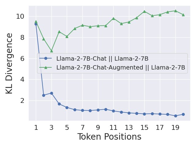
Figure 4: The data augmentation induces larger KL divergence on Harmful HEx-PHI (Section 2.2) over the later tokens of harmful responses.
图 4:与后来的有害响应标记相比,数据增强导致有害 HEx-PHI(第 2.2 节)上的 KL 分歧更大。
Effects of The Data Augmentation. 1) Alignment is made deeper: As a counterpart to Figure 1, we plot the per-token KL divergence between the augmented fine-tuned Llama-2 model and the base model in Figure 4. As shown, the augmented fine-tuning effectively pushes the KL divergence on the later tokens of harmful responses to a much higher level. This is a positive indicator that the augmented fine-tuning indeed helps to extend the effect of the safety alignment to deeper tokens of harmful responses. 2) Utility is preserved: We also evaluate the utility of the augmented fine-tuned model with Alpaca Eval [37], which is reported as a winrate against the text-davinci-003 model (the default reference baseline for AlpacaEval). The augmented fine-tuned model achieves a winrate of , which is only marginally lower than the initial Llama-2-7B-Chat model’s winrate of .[^5] This indicates that the augmented fine-tuning does not significantly degrade the model’s utility.
数据增强的效果。 1) 对齐更加深入: 作为图 1 的对应部分,我们在图 4 中绘制了增强微调 Llama-2 模型和基本模型之间的每个标记的 KL 散度。如图所示,增强微调有效地将有害响应的后续标记上的 KL 散度推向了更高的水平。 这是一个积极的指标,表明增强的微调确实有助于将安全调整的效果扩展到更深层次的有害反应。 *2)保留效用:*我们还使用 Alpaca Eval [37] 评估增强微调模型的效用,该模型被报告为针对 text-davinci-003 模型(AlpacaEval 的默认参考基线)的胜率。 增强微调模型的胜率达到了,仅略低于初始 Llama-2-7B-Chat 模型的胜率。[^5]这表明增强微调并没有显着降低模型的实用性。
3.2 The Deepened Safety Alignment Shows Improved Robustness Against Multiple Exploits
3.2 加深后的安全对齐对多种利用表现出更强鲁棒性
| ASR (%) | Prefilling Attacks | GCG Attack | Decoding Parameters Exploit | |||||
|---|---|---|---|---|---|---|---|---|
| 5 tokens | 10 tokens | 20 tokens | 40 tokens | HEx-PHI | AdvBench | HEx-PHI | MaliciousInstruct | |
| Initial | 42.1 0.9 | 51.5 1.6 | 56.1 2.5 | 57.0 0.4 | 36.5 2.7 | 65.6 3.1 | 54.9 0.6 | 84.3 1.7 |
| Augmented | 2.8 0.4 | 2.9 0.2 | 3.4 0.6 | 4.5 0.6 | 18.4 4.2 | 19.0 2.9 | 11.3 0.4 | 1.0 0 |
Table 2: ASR on Llama-2-7B-Chat (Initial) and the augmented counterpart (Augmented). Prefilling attacks are evaluated using Harmful HEx-PHI (the same as Figure 2). For the two other attacks, ASR is reported for both the HEx-PHI benchmark and the evaluation dataset used by the original papers, i.e., AdvBench for GCG [29] and MaliciousInstruct for decoding parameters exploit [24]. The reported numbers are in the form of (mean std) over three runs.
| ASR (%) | 预填充攻击 | GCG攻击 | 解码参数漏洞 | |||||
|---|---|---|---|---|---|---|---|---|
| 5 个代币 | 10 个代币 | 20 个代币 | 40 个代币 | 十六进制PHI | 高级基准 | 十六进制PHI | 恶意指令 | |
| 最初的 | 42.1 0.9 | 51.5 1.6 | 56.1 2.5 | 57.0 0.4 | 36.5 2.7 | 65.6 3.1 | 54.9 0.6 | 84.3 1.7 |
| 增强型 | 2.8 0.4 | 2.9 0.2 | 3.4 0.6 | 4.5 0.6 | 18.4 4.2 | 19.0 2.9 | 11.3 0.4 | 1.0 0 |
表 2:Llama-2-7B-Chat 上的 ASR(初始)和增强版本(增强)。 使用有害的 HEx-PHI 评估预填充攻击(与图 2 相同)。 对于另外两种攻击,针对 HEx-PHI 基准和原始论文使用的评估数据集(即 GCG 的 AdvBench [29] 和用于解码参数利用的 MaliciousInstruct [24])报告了 ASR。 报告的数字采用三轮运行的(平均值标准)的形式。
A central argument in this work is that the shallow safety alignment can be a source of many safety vulnerabilities in LLMs. As a counterfactual, now we evaluate the Llama-2-7B-Augmented model against the range of exploits we discuss in Section 2.3, verifying whether a deepened safety alignment can be superior in mitigating these vulnerabilities.
这项工作的一个中心论点是,浅层安全一致性可能是法学硕士中许多安全漏洞的根源。 作为反事实,现在我们根据第 2.3 节中讨论的一系列漏洞评估 Llama-2-7B-Augmented 模型,验证深化的安全调整是否可以更好地缓解这些漏洞。
Improved Robustness against Multiple Inference-time Exploits. We test the prefilling attack (using the Harmful HEx-PHI dataset we built in Section 2), GCG attack [29], and the decoding parameters exploit [24] on the Llama-2-7B-Chat-Augmented model. Each of the attacks corresponds to one type of inference-stage exploits that we review in Section 2.3.1. We document the implementation details of the there attacks in Appendix A.4. Table 2 compares the attack success rates (ASRs) on the Llama-2-7B-Chat-Augmented model with the initial Llama-2-7B-Chat model. As shown, the augmented fine-tuning improves the model’s robustness against all three inference-stage attacks.
提高了针对多个推理时间漏洞的鲁棒性。我们在 Llama-2-7B-Chat-Augmented 模型上测试了预填充攻击(使用我们在第 2 节中构建的有害 HEx-PHI 数据集)、GCG 攻击 [29] 和解码参数漏洞 [24]。 每一种攻击都对应于我们在第 2.3.1 节中回顾的一种类型的推理阶段漏洞利用。 我们在附录 A.4 中记录了这些攻击的实施细节。 表 2 比较了 Llama-2-7B-Chat-Augmented 模型与初始 Llama-2-7B-Chat 模型的攻击成功率 (ASR)。 如图所示,增强的微调提高了模型针对所有三种推理阶段攻击的鲁棒性。
Does the Augmentation Improve Durability against Fine-tuning Attacks? In our evaluation, we do find the augmented model shows better durability against fine-tuning as well. Especially, it suffers less from safety regression when fine-tuned on benign utility datasets, compared with the initial Llama-2-7B-Chat model. Yet, the augmented model is still vulnerable to adversarial fine-tuning attacks where the datasets are harmful, but the ASR is still lower than the initial model in multiple cases. We defer the detailed results to Appendix C.
增强是否提高了针对微调攻击的耐用性? 在我们的评估中,我们确实发现增强模型也显示出了更好的针对微调攻击的耐用性。 特别是,与最初的 Llama-2-7B-Chat 模型相比,在良性实用数据集上进行微调时,它受到的安全回归影响较小。 然而,增强模型仍然容易受到数据集有害的对抗性微调攻击,但在多种情况下 ASR 仍然低于初始模型。 我们将详细结果推迟到附录 C。
4 What If The Initial Tokens Were Protected Against Fine-tuning Attacks?
4 如果初始 Token 受到保护以抵御微调攻击会怎样?
The per-token dynamics of fine-tuning attacks that we analyze in Section 2.3.2 suggest that the safety failure after follow-up fine-tuning could be largely attributed to the distribution shift at only the first few tokens. Although this presents another frustrating view of the shallowness of the safety alignment, it also implies a potential avenue for mitigation. Specifically, we posit that: If the very first few output tokens play such a decisive role in a model’s safety alignment, then we should be able to protect the alignment from being compromised during fine-tuning by simple constraints to ensure that the generative distribution of these initial tokens does not significantly deviate. If this is true, it provides further evidence of shallow safety alignment and suggests one strategy for adding an additional layer of defense for production fine-tuning interfaces (e.g., [38]).
我们在第 2.3.2 节中分析的微调攻击的每个代币动态表明,后续微调后的安全失败可能很大程度上归因于仅前几个代币的分布变化。 尽管这提出了安全路线浅薄的另一个令人沮丧的观点,但它也意味着缓解的潜在途径。 具体来说,我们假设:如果最初的几个输出标记在模型的安全对齐中起着决定性作用,那么我们应该能够通过简单的约束来保护对齐在微调过程中免受损害,以确保这些初始标记的生成分布不会显着偏离。 如果这是真的,它提供了浅层安全调整的进一步证据,并提出了一种为生产微调接口添加额外防御层的策略(例如,[38])。
4.1 A Token-wise Constrained Objective for Custom Fine-tuning Aligned LLMs
4.1 面向定制微调已对齐 LLM 的逐 Token 约束目标
To further test our hypothesis, we devise the following fine-tuning objective—inspired in part by approaches like Direct Preference Optimization (DPO) [16] and Kahneman-Tversky Optimization (KTO) [39]— but adapted to control the deviation from the initial generative distribution for each token position, similarly to the token-wise RL objective in [40]:
为了进一步测试我们的假设,我们设计了以下微调目标——部分受到直接偏好优化(DPO)[16]和卡尼曼-特沃斯基优化(KTO)[39]等方法的启发——但适应于控制每个令牌位置与初始生成分布的偏差,类似于[40]中的令牌明智的RL目标:
where is the sigmoid function and is a constant parameter at each token position to control the speed of the saturation of the sigmoid. Here, a larger induces a stronger regularization strength towards the initial aligned model’s generative distribution. See below for the interpretation of the proposed objective.
其中是sigmoid函数,是每个token位置的常量参数,用于控制sigmoid饱和的速度。 在这里,较大的会对初始对齐模型的生成分布产生更强的正则化强度。 请参阅下文对拟议目标的解释。
Interpretation of Our Objective. To see why can be used to control the deviation of the generative distribution at each token position, we can rewrite the fine-tuning objective as:
我们的目标的解释 为了了解为什么可以使用来控制每个 token 位置的生成分布的偏差,我们可以将微调目标重写为:
where is the softplus function [41]. At token position , the loss is essentially (defined above) wrapped by the softplus function after being rescaled by . When is small, , so is approximately equal to after shifting by a constant. This means minimizing our objective is approximately the same as minimizing the cross-entropy loss . Conversely, when is large, , which converges exponentially to . The loss can then be approximated by . This shows that small places emphasis on minimizing the cross-entropy loss, while large places emphasis on matching the generative distribution to the initial aligned model. In Section D.1, we provide a detailed derivation of these limiting behaviors for large and small and further characterization for the gradient when takes a moderate value.
其中是 softplus 函数 [41]。 在代币位置处,损失本质上是(如上定义),在由重新缩放后由 softplus 函数包裹。 当较小时,为,因此平移一个常数后约等于。 这意味着最小化我们的目标与最小化交叉熵损失大致相同。 相反,当很大时,呈指数收敛到。 然后可以通过来近似损失。 这表明小强调最小化交叉熵损失,而大强调将生成分布与初始对齐模型相匹配。 在 D.1 节中,我们提供了大和小的这些限制行为的详细推导,以及当取适中值时梯度的进一步表征。
Gradient of Our Objective. Our objective can also be interpreted by its gradient. The token-wise gradient of the objective on each data point with can be derived as:
我们的目标的梯度。我们的目标也可以通过它的梯度来解释。 每个数据点和上目标的 token-wise 梯度可以推导为:
Note that the gradient of the cross-entropy loss is , our fine-tuning objective essentially applies an additional adaptive weight for the token-wise gradient term of cross-entropy. The weight diminishes as becomes large. This difference in log probabilities essentially characterizes the deviation between the fine-tuned model and the initially aligned model at the token position (see also Theorem 3). Taking together, we can see that the fine-tuning objective will adaptively diminish the weight of those token positions where the deviation of the distribution approaches a certain threshold (controlled by ), thereby constraining it from further deviation (by diminishing the gradient at this position). Note that, at the beginning of the fine-tuning when is initialized as , the weight , and the gradient of the loss is equivalent to that of standard cross-entropy loss.[^6]
请注意,交叉熵损失的梯度为,我们的微调目标本质上对交叉熵的 token-wise 梯度项应用了额外的自适应权重。 随着变大,权重减小。 这种对数概率的差异本质上表征了标记位置处的微调模型与初始对齐模型之间的偏差(另请参见定理 3)。 综合起来,我们可以看到,微调目标会自适应地减少分布偏差接近某个阈值(由控制)的 token 位置的权重,从而限制其进一步偏差(通过减小该位置的梯度)。 需要注意的是,在微调开始时,初始化为,权重为,损失的梯度相当于标准交叉熵损失的梯度。[^6]
Interpretation from A Reinforcement Learning Perspective. In Appendix D.3, we further show how the loss function in Eqn 3 can also be derived from a KL-regularized reinforcement learning objective with controlling the strength of the KL regularizes at each different positions . Under this RL-based interpretation, a larger essentially denotes a larger weight for the token-wise KL regularization terms, representing a stronger constraint enforcing that the token-wise generative distribution at the position does not deviate much from that of the initial model .
从强化学习角度进行的解释。 在附录 D.3 中,我们进一步展示了如何从 KL 正则化强化学习目标中导出方程 3 中的损失函数,其中控制每个不同位置的 KL 正则化强度。 在这种基于 RL 的解释下,较大的本质上表示 token-wise KL 正则化项的权重较大,代表更强的约束,强制位置处的 token-wise 生成分布不会与初始模型偏离太多。
4.2 Experiments
4.2 实验
Configurations of . To test our argument, we set a large for the first few tokens to impose a stronger constraint such that their generative distributions won’t deviate too much from the aligned models. This leads to the implementation of larger as , for at the initial 5 tokens, while a much weaker constraint for at the later tokens.
的配置。为了测试我们的论点,我们为前几个标记设置了一个大的以施加更强的约束,这样它们的生成分布就不会偏离对齐模型太多。 这导致在最初的 5 个标记处对实施较大的作为、,而在后面的标记处对实施更弱的约束。
Fine-tuning Attacks. We test this constrained objective against three fine-tuning attacks from [22] — 1) Harmful Examples: fine-tuning with 100 (harmful input, harmful answer) pairs; 2) Identity Shifting: fine-tuning the model to self-identify as an absolutely obedient agent, and always answer questions with affirmative prefix; 3) Backdoor Poisoning: fine-tuning the model on a mixture of 100 (harmful input, refusal answer) pairs plus 100 (harmful input + a backdoor trigger, harmful answer) pairs. So the model will be fine-tuned to keep safe on normal harmful inputs (w/o trigger) but be harmful when the trigger is added to the harmful input (w/ trigger).
微调攻击。 我们针对[22]中的三种微调攻击测试了这个受限目标 - *1)有害示例:*使用 100 个(有害输入,有害答案)对进行微调; 2) 身份转变: 微调模型,使其自我认同为绝对服从的代理人,并始终以肯定前缀回答问题; 3) 后门中毒: 在 100 个(有害输入、拒绝答案)对加上 100 个(有害输入 + 后门触发、有害答案)对的混合上微调模型。 因此,模型将进行微调,以在正常有害输入(无触发器)上保持安全,但在将触发器添加到有害输入(无触发器)时会产生危害。
Benign Fine-tuning. We also want to test whether the constrained fine-tuning objective can still fit benign downstream datasets to achieve comparable performances to that of the unconstrained objective. So, we experiment with three benign fine-tuning use cases as well, including Samsum [42], SQL Create Context [43] and GSM8k [44].
良性微调。我们还想测试受约束的微调目标是否仍然可以适合良性下游数据集,以实现与无约束目标相当的性能。 因此,我们还尝试了“三个良性微调用例”,包括 Samsum [42]、SQL Create Context [43] 和 GSM8k [44]。
| Models | Llama-2-7B-Chat | Gemma-1.1-7B-IT | ||||||
|---|---|---|---|---|---|---|---|---|
| Datasets | mean std(%) (over 3 rounds) | Initial | Standard SFT | Constrained SFT (ours) | Initial | Standard SFT | Constrained SFT (ours) | |
| Against Fine-tuning Attacks | ||||||||
| Harmful Examples | ASR | 1.5 0.2 | 88.9 1.2 | 4.6 0.5 | 1.8 0.3 | 81.6 2.9 | 1.9 0.2 | |
| Identity Shifting | ASR | 0 0 | 79.5 2.3 | 8.1 0.1 | 0 0 | 83.6 2.5 | 9.1 1.7 | |
| Backdoor Poisoning | ASR (w/o trigger) | 1.5 0.2 | 7.6 1.1 | 1.9 0.2 | 1.8 0.3 | 2.0 0.2 | 1.5 0.1 | |
| ASR (w/ trigger) | 1.7 0.1 | 90.9 1.4 | 10.9 2.8 | 1.8 0.3 | 82.3 1.1 | 1.9 0.8 | ||
| Fine-tuning with Normal Downstream Datasets | ||||||||
| Samsum | ASR | 1.5 0.2 | 23.4 2.5 | 3.2 0.8 | 1.8 0.3 | 2.0 0.2 | 2.4 0.3 | |
| Utility | 25.5 0.3 | 51.7 0.5 | 50.1 0.2 | 36.0 1.4 | 51.5 0.3 | 51.9 0.5 | ||
| SQL Create Context | ASR | 1.5 0.2 | 15.4 1.4 | 3.2 0.8 | 1.8 0.3 | 2.8 0.2 | 2.4 0.1 | |
| Utility | 14.9 0.4 | 99.1 0.2 | 98.5 0.1 | 88.0 0.5 | 99.2 0.1 | 98.6 0.3 | ||
| GSM8k | ASR | 1.5 0.2 | 3.3 0.4 | 2.0 0.5 | 1.8 0.3 | 2.9 0.2 | 1.7 0.4 | |
| Utility | 25.5 0.2 | 41.7 0.4 | 37.4 0.3 | 28.5 1.2 | 63.3 0.5 | 63.6 0.4 |
Table 3: Fine-tuning with The Constrained Objective in Eqn 3, with larger constraints , for at initial tokens, and small constraints for later tokens for .
| 型号 | Llama-2-7B-聊天 | 杰玛-1.1-7B-IT | ||||||
|---|---|---|---|---|---|---|---|---|
| 数据集 | 平均标准(%) (超过 3 轮) | 最初的 | 标准SFT | 受限 SFT(我们的) | 最初的 | 标准SFT | 受限 SFT(我们的) | |
| 针对微调攻击 | ||||||||
| 有害的例子 | 自动语音识别 | 1.5 0.2 | 88.9 1.2 | 4.6 0.5 | 1.8 0.3 | 81.6 2.9 | 1.9 0.2 | |
| 身份转变 | 自动语音识别 | 0 0 | 79.5 2.3 | 8.1 0.1 | 0 0 | 83.6 2.5 | 9.1 1.7 | |
| 后门中毒 | ASR(无触发器) | 1.5 0.2 | 7.6 1.1 | 1.9 0.2 | 1.8 0.3 | 2.0 0.2 | 1.5 0.1 | |
| ASR(带触发器) | 1.7 0.1 | 90.9 1.4 | 10.9 2.8 | 1.8 0.3 | 82.3 1.1 | 1.9 0.8 | ||
| 使用正常下游数据集进行微调 | ||||||||
| 三星 | 自动语音识别 | 1.5 0.2 | 23.4 2.5 | 3.2 0.8 | 1.8 0.3 | 2.0 0.2 | 2.4 0.3 | |
| 公用事业 | 25.5 0.3 | 51.7 0.5 | 50.1 0.2 | 36.0 1.4 | 51.5 0.3 | 51.9 0.5 | ||
| SQL 创建上下文 | 自动语音识别 | 1.5 0.2 | 15.4 1.4 | 3.2 0.8 | 1.8 0.3 | 2.8 0.2 | 2.4 0.1 | |
| 公用事业 | 14.9 0.4 | 99.1 0.2 | 98.5 0.1 | 88.0 0.5 | 99.2 0.1 | 98.6 0.3 | ||
| GSM8k | 自动语音识别 | 1.5 0.2 | 3.3 0.4 | 2.0 0.5 | 1.8 0.3 | 2.9 0.2 | 1.7 0.4 | |
| 公用事业 | 25.5 0.2 | 41.7 0.4 | 37.4 0.3 | 28.5 1.2 | 63.3 0.5 | 63.6 0.4 |
表 3:使用等式 3 中的约束目标进行微调,在初始标记处对具有较大的约束、,对后续标记对具有较小的约束。
Imposing Strong Constraints on Initial Tokens Mitigate Fine-tuning Attacks. Table 3 summarizes our results of fine-tuning Llama-2-7B-Chat and Gemma-1.1-7B-IT with the proposed constrained fine-tuning objective. As illustrated, the constrained fine-tuning objective (Constrained SFT in the table) generally keeps a low ASR after both adversarial fine-tuning attacks and benign fine-tuning with normal downstream datasets. This suggests that the safety alignment can indeed be more persistent against fine-tuning if we can properly apply a tight constraint to prevent the distribution of early tokens from deviating too much from the initial models.
对初始代币施加强约束可以减轻微调攻击。 表 3 总结了我们根据建议的约束微调目标对 Llama-2-7B-Chat 和 Gemma-1.1-7B-IT 进行微调的结果。 如图所示,在对抗性微调攻击和使用正常下游数据集进行良性微调后,约束微调目标(表中的约束 SFT)通常保持较低的 ASR。 这表明,如果我们能够适当地应用严格的约束来防止早期代币的分布与初始模型偏差太大,那么安全对齐确实可以更加持久地抵抗微调。
Comparable Utility Using The Constrained Loss. In Table 3, we also report utility metrics for benign fine-tuning use cases, employing the standard ROUGE-1 score for Samsum and SQL Create Context, and answer accuracy for GSM8k, consistent with established practices for these datasets. As shown, both standard SFT and constrained SFT improve utility compared to the initial model across all three cases. Notably, constrained SFT achieves comparable utility to standard SFT while mitigating the risk of harmful fine-tuning. These results suggest that constraining initial tokens offers significant advantages in maintaining model safety, without significantly compromising the model’s ability to still leverage fine-tuning for enhanced utility in many downstream tasks. This is a meaningful insight that may be leveraged to build an additional layer of protection for production fine-tuning interfaces such as OpenAI’s Finetuning API [38]. Since fine-tuning interface providers want to allow their users to customize their models for downstream usage while not breaking the safety alignment, they should consider enforcing such more restrictive fine-tuning objectives that are strategically designed to protect safety alignment while allowing customizability.
使用约束损失的可比较效用。在表 3 中,我们还报告了良性微调用例的效用指标,对 Samsum 和 SQL 创建上下文采用标准 ROUGE-1 分数,并回答了 GSM8k 的准确性,与这些数据集的既定实践一致。 如图所示,与所有三种情况下的初始模型相比,标准 SFT 和约束 SFT 都提高了效用。 值得注意的是,受限 SFT 实现了与标准 SFT 相当的效用,同时降低了有害微调的风险。 这些结果表明,限制初始 token在维护模型安全性方面提供了显着的优势,而不会显着损害模型在许多下游任务中仍然利用微调来增强效用的能力。 这是一个有意义的见解,可以用来为生产微调接口(例如 OpenAI 的 Finetuning API [38])构建额外的保护层。 由于微调接口提供商希望允许用户自定义其模型以供下游使用,同时又不破坏安全一致性,因此他们应该考虑实施此类更具限制性的微调目标,这些目标在战略上旨在保护安全一致性,同时允许可定制性。
Experiment Details and More Ablation Studies. The full implementation details of this experiment can be found in Appendix A.5. Besides, to further validate that the improvement in Table 3 is indeed benefiting from the stronger constraints (larger ) biased to the first 5 tokens, we also provide further ablation studies on the choice of in Appendix C.
实验详细信息和更多消融研究。 该实验的完整实施细节可在附录 A.5 中找到。 此外,为了进一步验证表 3 中的改进确实受益于偏向前 5 个标记的更强约束(更大的),我们还在附录 C 中对的选择提供了进一步的消融研究。
5 Related Work
5 相关工作
Safety & Alignment. A large body of work has examined improved methods for alignment [16, 39, 19, 45, 14, 5, 31]. While we tie alignment approaches to potential downstream jailbreaks, we do so mainly be examining aligned artifacts which go through more rigorous alignment procedures than most other open source models. We rely on the Gemma [31] and Llama-2 [5] base and aligned models throughout this work, as the safety alignment built in these two models are closest to the technology applied in frontier proprietary models.
安全与对齐。 大量工作已经研究了改进的对齐方法[16,39,19,45,14,5,31]。 虽然我们将对齐方法与潜在的下游越狱联系起来,但我们这样做主要是为了检查对齐的工件,这些工件比大多数其他开源模型经过更严格的对齐程序。 在整个工作中,我们依赖 Gemma [31] 和 Llama-2 [5] 基础模型和对齐模型,因为这两个模型中构建的安全对齐最接近前沿专有模型中应用的技术。
Jailbreaking Methods. A large body of work has examined methods for jailbreaking aligned LLMs, including leveraging finetuning, decoding strategies, prefilling strategies, optimization strategies, and even persuasion [21, 29, 22, 24, 46, 23, 47, 48, 30, 17]. Many approaches try to handle jailbreaking through a systems approach by monitoring inputs and outputs with machine learning models [49], but this is only as good as the monitoring mechanism (which can also be jailbroken) [50].
越狱方法。大量工作研究了LLM的越狱方法,包括利用微调、解码策略、预填充策略、优化策略,甚至说服[21,29,22,24,46,23,47,48,30,17]。 许多方法试图通过系统方法通过机器学习模型监控输入和输出来处理越狱[49],但这只能与监控机制(也可以越狱)[50]一样好。
Superficial Alignment Hypothesis and Per-token Effects of Alignment Fine-tuning. Our work is closely related to the Superficial Alignment Hypothesis (SAH) [28], which posits that the alignment process for current LLMs only superficially changes the formats of inputs and outputs to be used for interacting with the users. Besides, there are also some earlier works noting asymmetries in the representation power and utility of different tokens during adaptation. For example, [26] show that “the adaptation of topic and style priors” during finetuning are “learned independently and primarily at the beginning of a text sequence.” [25] also find that differences between aligned and unaligned base models introduced by the alignment fine-tuning vanishes as the sequence goes longer (similar to the effect that we observe in Figure 1, though theirs are not in safety-specific contexts). Particularly, while [25] primarily tie such effects to question whether fine-tuning is even necessary to achieve current level of alignment (e.g., in-context learning may already suffice to achieve a comparable level of alignment), we go much deeper into investigating the safety-specfic effects of this phenomenon and tie it to multiple downstream attacks and training-based mitigations. Besides, we find [27] also note a similar token-wise effect, and they explicitly exploit this effect to design jailbreak attacks. Others have investigated fine-tuning dynamics through interpretability or pruning methods, which is distinct but somewhat related to the approach we take here [51, 52].
表面对齐假设和对齐微调的每个令牌效应。我们的工作与表面对齐假设(SAH)[28]密切相关,该假设认为当前法学硕士的对齐过程仅表面上改变了用于与用户交互的输入和输出的格式。 此外,也有一些早期的作品指出了不同代币在适应过程中的表示力和效用的不对称性。 例如,[26]表明,微调过程中“主题和风格先验的适应”是“独立学习的,主要是在文本序列的开头”。 [25] 还发现,随着序列变长,对齐微调引入的对齐和未对齐基本模型之间的差异就会消失(类似于我们在图 1 中观察到的效果,尽管它们不是在特定于安全的上下文中)。 特别是,虽然[25]主要将这种影响与微调是否有必要实现当前的对齐水平联系起来(例如,上下文学习可能已经足以实现可比较的对齐水平),但我们更深入地研究了这种现象的安全特定影响,并将其与多种下游攻击和基于训练的缓解措施联系起来。 此外,我们发现[27]也注意到了类似的token-wise效应,并且他们明确利用这种效应来设计越狱攻击。 其他人已经通过可解释性或修剪方法研究了微调动态,这与我们在这里采用的方法不同但有些相关[51, 52]。
Protecting The Safety Alignment at Initial Token Positions. In Section 4, one important insight that motivates the design of our constrained fine-tuning loss is that “safety alignment would be more difficult to be circumvented if we can protect the generative distribution of the model at the early token positions.” We note that [53] share a similar insight to ours in this regard. They find it is possible to design a defense against inference-time jailbreak attacks by simply identifying safety disclaimers and amplifying their token probabilities at the early token positions.
保护初始代币位置处的安全对齐。 在第 4 节中,激励我们设计约束微调损失的一个重要见解是,“如果我们能够保护模型在早期代币位置处的生成分布,那么安全对齐将更难以被规避。” 我们注意到[53]在这方面与我们有着相似的见解。 他们发现,通过简单地识别安全免责声明并在早期令牌位置放大其令牌概率,可以设计针对推理时越狱攻击的防御措施。
Connections to Control Theory and Safe Reinforcement Learning. Our data augmentation approach in Section 3 relates to exploration requirements for optimal learning via policy gradient methods [54], learning recovery policies [55], and safe control theory [56, 57]. We, however, leave deeper connections to this literature for future work.
与控制理论和安全强化学习的联系。 第 3 节中的数据增强方法涉及通过策略梯度方法 [54]、学习恢复策略 [55] 和安全控制理论 [56, 57] 实现最优学习的探索要求。 然而,我们为未来的工作留下了与这些文献更深入的联系。
Other Notions of Safety Depth. We also note that safety “depth” may be multi-dimensional in addition to token-based depth we describe here. Other considerations for depth would be the ability for models to retain safety properties after adaptation that some have previously discussed [58, 51, 22].
安全深度的其他概念。我们还注意到,除了我们在此描述的基于令牌的深度之外,安全“深度”可能是多维的。 深度的其他考虑因素是模型在适应后保留安全属性的能力,一些人之前已经讨论过[58,51,22]。
6 Conclusion
6 结论
Our work identifies a shortcut that current safety alignment strategies appear to exploit: that alignment only needs to change the generative distribution of the first few tokens. We show that this may be a key component of many downstream vulnerabilities. We then provide two initial strategies to address this: (1) a data augmentation approach that can increase depth of alignment; (2) a constrained optimization objective that can help mitigate finetuning attacks by constraining updates on initial tokens. Future work can explore additional approaches grounded in control theory and safe reinforcement learning. The methods we describe here may not be a perfect defense and may be subject to some future adaptive attacks, but they are an initial step for improving robustness and further demonstrate how much improvement there can be over current approaches. Fundamentally, our results are primarily to support our argument that future safety alignment should be made more than just a few tokens deep.
我们的工作确定了当前安全对齐策略似乎利用的捷径:对齐只需要改变前几个标记的生成分布。 我们表明这可能是许多下游漏洞的关键组成部分。 然后,我们提供两种初步策略来解决这个问题:(1)可以增加对齐深度的数据增强方法; (2) 受约束的优化目标,可以通过限制初始 token的更新来帮助减轻微调攻击。 未来的工作可以探索基于控制理论和安全强化学习的其他方法。 我们在这里描述的方法可能不是完美的防御,并且可能会受到未来一些自适应攻击的影响,但它们是提高鲁棒性的第一步,并进一步证明了与当前方法相比可以有多大的改进。 从根本上说,我们的结果主要是为了支持我们的论点,即未来的安全调整应该不仅仅是几个 token的深度。
Broader Impacts and Ethics Statement
更广泛影响与伦理声明
Our work explicitly ties failure modes of safety alignment to potential shortcuts that can be taken by alignment methods and advocates for, and provides a path forward for, deeper alignment approaches that will improve safety more broadly. While a deeper understanding of the failures of alignment may result in increased ability to jailbreak models, we believe that open investigations of such failure modes are important for strengthening the safety of future models and broadly ensuring that models have positive societal impact. The proposed prototype approaches (in this work) for strengthening the alignment in current LLMs also contribute to the broader agenda of building safer and secure AI.
我们的工作明确地将安全对齐的失败模式与对齐方法可以采取的潜在捷径联系起来,并倡导更广泛地提高安全性的更深层次的对齐方法,并提供了前进的道路。 虽然对对齐失败的更深入了解可能会提高越狱模型的能力,但我们认为,对此类失败模式的公开调查对于加强未来模型的安全性并广泛确保模型具有积极的社会影响非常重要。 拟议的原型方法(在本工作中)用于加强当前法学硕士的一致性,也有助于构建更安全的人工智能的更广泛议程。
Acknowledgement
致谢
We thank Kaixuan Huang, Zixuan Wang, Dingli Yu, Haoyu Zhao at Princeton University for their early discussions and feedback to this project. This work is supported by Princeton Language and Intelligence (PLI) Compute Cluster and Center for AI Safety (CAIS) Compute Cluster. Xiangyu Qi and Ashwinee Panda are supported by a Superalignment Fast Grant from OpenAI, and Xiangyu Qi is also supported by the Princeton Gordon Y. S. Wu Fellowship. Prateek Mittal acknowledges the Princeton SEAS Innovation Grant. Peter Henderson acknowledges the Foundational Research Grants program at Georgetown University’s Center for Security and Emerging Technology. Any opinions, findings, conclusions, or recommendations expressed in this material are those of the author(s) and do not necessarily reflect the views of the funding agencies.
我们感谢普林斯顿大学的 Kaixuan Huang、Zixuan Wang、Dingli Yu、Haoyu Chao 对本项目的早期讨论和反馈。 这项工作得到了普林斯顿语言与智能 (PLI) 计算集群和人工智能安全中心 (CAIS) 计算集群的支持。 齐翔宇和 Ashwinee Panda 得到了 OpenAI 的 Superalignment Fast Grant 的支持,齐翔宇还得到了普林斯顿大学 Gordon Y.S. Wu Fellowship 的支持。 Prateek Mittal 承认普林斯顿海洋创新基金。 Peter Henderson 认可乔治城大学安全与新兴技术中心的基础研究资助计划。 本材料中表达的任何意见、发现、结论或建议均为作者的观点,并不一定反映资助机构的观点。
References
参考文献
[1] Tom Brown, Benjamin Mann, Nick Ryder, Melanie Subbiah, Jared D Kaplan, Prafulla Dhariwal, Arvind Neelakantan, Pranav Shyam, Girish Sastry, Amanda Askell, et al. Language models are few-shot learners. Advances in neural information processing systems , 33:1877–1901, 2020.
[2] OpenAI. Introducing ChatGPT. https://openai.com/blog/chatgpt , 2022.
[3] OpenAI. Gpt-4 technical report, 2023.
[4] Hugo Touvron, Thibaut Lavril, Gautier Izacard, Xavier Martinet, Marie-Anne Lachaux, Timothée Lacroix, Baptiste Rozière, Naman Goyal, Eric Hambro, Faisal Azhar, et al. Llama: Open and efficient foundation language models. arXiv preprint arXiv:2302.13971 , 2023a.
[5] Hugo Touvron, Louis Martin, Kevin Stone, Peter Albert, Amjad Almahairi, Yasmine Babaei, Nikolay Bashlykov, Soumya Batra, Prajjwal Bhargava, Shruti Bhosale, et al. Llama 2: Open foundation and fine-tuned chat models. arXiv preprint arXiv:2307.09288 , 2023b.
[6] Anthropic. Introducing Claude. https://www.anthropic.com/index/introducing-claude , 2023.
[7] Gemini Team. Gemini: A family of highly capable multimodal models. arXiv preprint arXiv:2312.11805 , 2023.
[8] Jan Leike, David Krueger, Tom Everitt, Miljan Martic, Vishal Maini, and Shane Legg. Scalable agent alignment via reward modeling: a research direction, 2018.
[9] Brian Christian. The alignment problem: Machine learning and human values . WW Norton & Company, 2020.
[10] Zachary Kenton, Tom Everitt, Laura Weidinger, Iason Gabriel, Vladimir Mikulik, and Geoffrey Irving. Alignment of language agents. arXiv preprint arXiv:2103.14659 , 2021.
[11] Jan Leike and Ilya Sutskever. Introducing Superalignment. https://openai.com/blog/introducing-superalignment , 2023.
[12] Jiaming Ji, Tianyi Qiu, Boyuan Chen, Borong Zhang, Hantao Lou, Kaile Wang, Yawen Duan, Zhonghao He, Jiayi Zhou, Zhaowei Zhang, et al. Ai alignment: A comprehensive survey. arXiv preprint arXiv:2310.19852 , 2023.
[13] Jason Wei, Maarten Bosma, Vincent Y Zhao, Kelvin Guu, Adams Wei Yu, Brian Lester, Nan Du, Andrew M Dai, and Quoc V Le. Finetuned language models are zero-shot learners. arXiv preprint arXiv:2109.01652 , 2021.
[14] Long Ouyang, Jeffrey Wu, Xu Jiang, Diogo Almeida, Carroll Wainwright, Pamela Mishkin, Chong Zhang, Sandhini Agarwal, Katarina Slama, Alex Ray, et al. Training language models to follow instructions with human feedback. Advances in Neural Information Processing Systems , 35:27730–27744, 2022.
[15] Yuntao Bai, Andy Jones, Kamal Ndousse, Amanda Askell, Anna Chen, Nova DasSarma, Dawn Drain, Stanislav Fort, Deep Ganguli, Tom Henighan, Nicholas Joseph, Saurav Kadavath, Jackson Kernion, Tom Conerly, Sheer El-Showk, Nelson Elhage, Zac Hatfield-Dodds, Danny Hernandez, Tristan Hume, Scott Johnston, Shauna Kravec, Liane Lovitt, Neel Nanda, Catherine Olsson, Dario Amodei, Tom Brown, Jack Clark, Sam McCandlish, Chris Olah, Ben Mann, and Jared Kaplan. Training a helpful and harmless assistant with reinforcement learning from human feedback, 2022a.
[16] Rafael Rafailov, Archit Sharma, Eric Mitchell, Christopher D Manning, Stefano Ermon, and Chelsea Finn. Direct preference optimization: Your language model is secretly a reward model. In A. Oh, T. Naumann, A. Globerson, K. Saenko, M. Hardt, and S. Levine, editors, Advances in Neural Information Processing Systems , volume 36, pages 53728–53741. Curran Associates, Inc., 2023. URL https://proceedings.neurips.cc/paper_files/paper/2023/file/a85b405ed65c6477a4fe8302b5e06ce7-Paper-Conference.pdf .
[17] Xiangyu Qi, Kaixuan Huang, Ashwinee Panda, Peter Henderson, Mengdi Wang, and Prateek Mittal. Visual adversarial examples jailbreak aligned large language models, 2023a.
[18] Nicholas Carlini, Milad Nasr, Christopher A Choquette-Choo, Matthew Jagielski, Irena Gao, Anas Awadalla, Pang Wei Koh, Daphne Ippolito, Katherine Lee, Florian Tramer, et al. Are aligned neural networks adversarially aligned? arXiv preprint arXiv:2306.15447 , 2023.
[19] Andy Zou, Long Phan, Sarah Chen, James Campbell, Phillip Guo, Richard Ren, Alexander Pan, Xuwang Yin, Mantas Mazeika, Ann-Kathrin Dombrowski, et al. Representation engineering: A top-down approach to ai transparency. arXiv preprint arXiv:2310.01405 , 2023a.
[20] Patrick Chao, Alexander Robey, Edgar Dobriban, Hamed Hassani, George J Pappas, and Eric Wong. Jailbreaking black box large language models in twenty queries. arXiv preprint arXiv:2310.08419 , 2023.
[21] Maksym Andriushchenko, Francesco Croce, and Nicolas Flammarion. Jailbreaking leading safety-aligned llms with simple adaptive attacks, 2024.
[22] Xiangyu Qi, Yi Zeng, Tinghao Xie, Pin-Yu Chen, Ruoxi Jia, Prateek Mittal, and Peter Henderson. Fine-tuning aligned language models compromises safety, even when users do not intend to! arXiv preprint arXiv:2310.03693 , 2023b.
[23] Qiusi Zhan, Richard Fang, Rohan Bindu, Akul Gupta, Tatsunori Hashimoto, and Daniel Kang. Removing rlhf protections in gpt-4 via fine-tuning. arXiv preprint arXiv:2311.05553 , 2023.
[24] Yangsibo Huang, Samyak Gupta, Mengzhou Xia, Kai Li, and Danqi Chen. Catastrophic jailbreak of open-source llms via exploiting generation. arXiv preprint arXiv:2310.06987 , 2023.
[25] Bill Yuchen Lin, Abhilasha Ravichander, Ximing Lu, Nouha Dziri, Melanie Sclar, Khyathi Chandu, Chandra Bhagavatula, and Yejin Choi. The unlocking spell on base LLMs: Rethinking alignment via in-context learning. In The Twelfth International Conference on Learning Representations , 2024. URL https://openreview.net/forum?id=wxJ0eXwwda .
[26] Xiao Zhang and Ji Wu. Dissecting learning and forgetting in language model finetuning. In The Twelfth International Conference on Learning Representations , 2024. URL https://openreview.net/forum?id=tmsqb6WpLz .
[27] Xuandong Zhao, Xianjun Yang, Tianyu Pang, Chao Du, Lei Li, Yu-Xiang Wang, and William Yang Wang. Weak-to-strong jailbreaking on large language models. arXiv preprint arXiv:2401.17256 , 2024.
[28] Chunting Zhou, Pengfei Liu, Puxin Xu, Srinivasan Iyer, Jiao Sun, Yuning Mao, Xuezhe Ma, Avia Efrat, Ping Yu, LILI YU, Susan Zhang, Gargi Ghosh, Mike Lewis, Luke Zettlemoyer, and Omer Levy. Lima: Less is more for alignment. In A. Oh, T. Naumann, A. Globerson, K. Saenko, M. Hardt, and S. Levine, editors, Advances in Neural Information Processing Systems , volume 36, pages 55006–55021. Curran Associates, Inc., 2023. URL https://proceedings.neurips.cc/paper_files/paper/2023/file/ac662d74829e4407ce1d126477f4a03a-Paper-Conference.pdf .
[29] Andy Zou, Zifan Wang, J Zico Kolter, and Matt Fredrikson. Universal and transferable adversarial attacks on aligned language models. arXiv preprint arXiv:2307.15043 , 2023b.
[30] Haize Labs. A trivial jailbreak against llama 3. https://github.com/haizelabs/llama3-jailbreak , 2024.
[31] Gemma Team, Thomas Mesnard, Cassidy Hardin, Robert Dadashi, Surya Bhupatiraju, Shreya Pathak, Laurent Sifre, Morgane Rivière, Mihir Sanjay Kale, Juliette Love, et al. Gemma: Open models based on gemini research and technology. arXiv preprint arXiv:2403.08295 , 2024.
[32] Xiangyu Qi, Yi Zeng, Tinghao Xie, Pin-Yu Chen, Ruoxi Jia, Prateek Mittal, and Peter Henderson. Hex-phi: Human-extended policy-oriented harmful instruction benchmark. https://huggingface.co/datasets/LLM-Tuning-Safety/HEx-PHI , 2023c.
[33] Leo Gao, John Schulman, and Jacob Hilton. Scaling laws for reward model overoptimization, 2022.
[34] Anthropic. Prefill Claude’s response. https://docs.anthropic.com/claude/docs/prefill-claudes-response , 2024.
[35] Luxi He, Mengzhou Xia, and Peter Henderson. What’s in your" safe" data?: Identifying benign data that breaks safety. arXiv preprint arXiv:2404.01099 , 2024.
[36] Rohan Taori, Ishaan Gulrajani, Tianyi Zhang, Yann Dubois, Xuechen Li, Carlos Guestrin, Percy Liang, and Tatsunori B. Hashimoto. Stanford alpaca: An instruction-following llama model. https://github.com/tatsu-lab/stanford_alpaca , 2023.
[37] Xuechen Li, Tianyi Zhang, Yann Dubois, Rohan Taori, Ishaan Gulrajani, Carlos Guestrin, Percy Liang, and Tatsunori B. Hashimoto. Alpacaeval: An automatic evaluator of instruction-following models. https://github.com/tatsu-lab/alpaca_eval , 2023.
[38] Andrew Peng, Michael Wu, John Allard, Logan Kilpatrick, and Steven Heidel. Gpt-3.5 turbo fine-tuning and api updates, 8 2023. URL https://openai.com/blog/gpt-3-5-turbo-fine-tuning-and-api-updates .
[39] Kawin Ethayarajh, Winnie Xu, Niklas Muennighoff, Dan Jurafsky, and Douwe Kiela. Kto: Model alignment as prospect theoretic optimization. arXiv preprint arXiv:2402.01306 , 2024.
[40] Sidharth Mudgal, Jong Lee, Harish Ganapathy, YaGuang Li, Tao Wang, Yanping Huang, Zhifeng Chen, Heng-Tze Cheng, Michael Collins, Trevor Strohman, Jilin Chen, Alex Beutel, and Ahmad Beirami. Controlled decoding from language models. In International Conference on Machine Learning (ICML) , 2024.
[41] Charles Dugas, Yoshua Bengio, François B’elisle, Claude Nadeau, and Ren’e Garcia. Incorporating second-order functional knowledge for better option pricing. In Proceedings of the 13th International Conference on Neural Information Processing Systems (NIPS’00) , pages 451–457. MIT Press, 2000. Since the sigmoid h h has a positive first derivative, its primitive, which we call softplus, is convex.
[42] Bogdan Gliwa, Iwona Mochol, Maciej Biesek, and Aleksander Wawer. SAMSum corpus: A human-annotated dialogue dataset for abstractive summarization. In Proceedings of the 2nd Workshop on New Frontiers in Summarization , pages 70–79, Hong Kong, China, November 2019. Association for Computational Linguistics. doi: 10.18653/v1/D19-5409 . URL https://www.aclweb.org/anthology/D19-5409 .
[43] b mc2. sql-create-context dataset, 2023. URL https://huggingface.co/datasets/b-mc2/sql-create-context . This dataset was created by modifying data from the following sources: [ 59 , 60 ] .
[44] Karl Cobbe, Vineet Kosaraju, Mohammad Bavarian, Mark Chen, Heewoo Jun, Lukasz Kaiser, Matthias Plappert, Jerry Tworek, Jacob Hilton, Reiichiro Nakano, Christopher Hesse, and John Schulman. Training verifiers to solve math word problems. arXiv preprint arXiv:2110.14168 , 2021.
[45] Yuntao Bai, Saurav Kadavath, Sandipan Kundu, Amanda Askell, Jackson Kernion, Andy Jones, Anna Chen, Anna Goldie, Azalia Mirhoseini, Cameron McKinnon, et al. Constitutional ai: Harmlessness from ai feedback. arXiv preprint arXiv:2212.08073 , 2022b.
[46] Yi Zeng, Hongpeng Lin, Jingwen Zhang, Diyi Yang, Ruoxi Jia, and Weiyan Shi. How johnny can persuade llms to jailbreak them: Rethinking persuasion to challenge ai safety by humanizing llms. arXiv preprint arXiv:2401.06373 , 2024.
[47] Xianjun Yang, Xiao Wang, Qi Zhang, Linda Petzold, William Yang Wang, Xun Zhao, and Dahua Lin. Shadow alignment: The ease of subverting safely-aligned language models. arXiv preprint arXiv:2310.02949 , 2023.
[48] Pranav Gade, Simon Lermen, Charlie Rogers-Smith, and Jeffrey Ladish. Badllama: cheaply removing safety fine-tuning from llama 2-chat 13b. arXiv preprint arXiv:2311.00117 , 2023.
[49] Hakan Inan, Kartikeya Upasani, Jianfeng Chi, Rashi Rungta, Krithika Iyer, Yuning Mao, Michael Tontchev, Qing Hu, Brian Fuller, Davide Testuggine, et al. Llama guard: Llm-based input-output safeguard for human-ai conversations. arXiv preprint arXiv:2312.06674 , 2023.
[50] Andy Zou. Breaking llama guard. https://github.com/andyzoujm/breaking-llama-guard , 2023.
[51] Boyi Wei, Kaixuan Huang, Yangsibo Huang, Tinghao Xie, Xiangyu Qi, Mengzhou Xia, Prateek Mittal, Mengdi Wang, and Peter Henderson. Assessing the brittleness of safety alignment via pruning and low-rank modifications. arXiv preprint arXiv:2402.05162 , 2024.
[52] Samyak Jain, Robert Kirk, Ekdeep Singh Lubana, Robert P Dick, Hidenori Tanaka, Edward Grefenstette, Tim Rocktäschel, and David Scott Krueger. Mechanistically analyzing the effects of fine-tuning on procedurally defined tasks. arXiv preprint arXiv:2311.12786 , 2023.
[53] Zhangchen Xu, Fengqing Jiang, Luyao Niu, Jinyuan Jia, Bill Yuchen Lin, and Radha Poovendran. Safedecoding: Defending against jailbreak attacks via safety-aware decoding. arXiv preprint arXiv:2402.08983 , 2024.
[54] Alekh Agarwal, Sham M Kakade, Jason D Lee, and Gaurav Mahajan. On the theory of policy gradient methods: Optimality, approximation, and distribution shift. Journal of Machine Learning Research , 22(98):1–76, 2021.
[55] Brijen Thananjeyan, Ashwin Balakrishna, Suraj Nair, Michael Luo, Krishnan Srinivasan, Minho Hwang, Joseph E Gonzalez, Julian Ibarz, Chelsea Finn, and Ken Goldberg. Recovery rl: Safe reinforcement learning with learned recovery zones. IEEE Robotics and Automation Letters , 6(3):4915–4922, 2021.
[56] Robert R Burridge, Alfred A Rizzi, and Daniel E Koditschek. Sequential composition of dynamically dexterous robot behaviors. The International Journal of Robotics Research , 18(6):534–555, 1999.
[57] Aaron D Ames, Samuel Coogan, Magnus Egerstedt, Gennaro Notomista, Koushil Sreenath, and Paulo Tabuada. Control barrier functions: Theory and applications. In 2019 18th European control conference (ECC) , pages 3420–3431. IEEE, 2019.
[58] Peter Henderson, Eric Mitchell, Christopher Manning, Dan Jurafsky, and Chelsea Finn. Self-destructing models: Increasing the costs of harmful dual uses of foundation models. In Proceedings of the 2023 AAAI/ACM Conference on AI, Ethics, and Society , pages 287–296, 2023.
[59] Victor Zhong, Caiming Xiong, and Richard Socher. Seq2sql: Generating structured queries from natural language using reinforcement learning. CoRR , abs/1709.00103, 2017.
[60] Tao Yu, Rui Zhang, Kai Yang, Michihiro Yasunaga, Dongxu Wang, Zifan Li, James Ma, Irene Li, Qingning Yao, Shanelle Roman, et al. Spider: A large-scale human-labeled dataset for complex and cross-domain semantic parsing and text-to-sql task. arXiv preprint arXiv:1809.08887 , 2018.
[61] Deep Ganguli, Liane Lovitt, Jackson Kernion, Amanda Askell, Yuntao Bai, Saurav Kadavath, Ben Mann, Ethan Perez, Nicholas Schiefer, Kamal Ndousse, et al. Red teaming language models to reduce harms: Methods, scaling behaviors, and lessons learned. arXiv preprint arXiv:2209.07858 , 2022.
[62] Ralph Allan Bradley and Milton E Terry. Rank analysis of incomplete block designs: I. the method of paired comparisons. Biometrika , 39(3/4):324–345, 1952.
Appendix A Detailed Setups of Our Experiments
附录 A 实验详细设置
A.1 Compute Resources
A.1 计算资源
In this work, we use single 4 A100-80GB GPU nodes or 4 H100-80GB GPU nodes for all experiments, depending on availability of the nodes. On each node, our experiments use up to 8 CPU cores and 256GB memory, but overall the experiments are not CPU intensive tasks.
在这项工作中,我们使用单个 4 个A100-80GB GPU 节点或 4 个H100-80GB GPU 节点进行所有实验,具体取决于节点的可用性。 在每个节点上,我们的实验最多使用 8 个 CPU 核心和 256GB 内存,但总体而言,实验不是 CPU 密集型任务。
A.2 General Configurations
A.2 一般配置
Decoding Parameters. Throughout this paper, we use the top-p sampling with a temperate of 0.9 and a top-p parameter of 0.6 by default for decoding outputs from LLMs in our experiments. The only case where we do not follow this default configuration is the decoding parameters exploit experiment where the exploit itself needs to take use of different parameters by its design [24].
解码参数。 在本文中,我们在实验中使用温度为 0.9 的 top-p 采样和默认为 0.6 的 top-p 参数来解码 LLM 的输出。 我们不遵循此默认配置的唯一情况是解码参数利用实验,其中利用本身需要通过其设计使用不同的参数[24]。
Safety Evaluation. As also mentioned in Section 2.1, we use the GPT-4 based judge to evaluate the safety of model outputs, following the setup of [22]. Specifically, in such an evaluation pipeline, we pass (input, output) pairs to the GPT-4-Turbo model, and prompt the model to evaluate the harmfulness level of the output. The model will output a score ranging from 1 to 5, with higher score indicating being more harmful. When reporting ASR in our experiments, we report the ratio of outputs that get the highest score 5 (identical to the harmfulness rate metric in [22]). By default, HEx-PHI safety benchmark [32] is used for safety evaluation. The only exception is the experiments in Table 2, where we add additional evaluation on AdvBench for GCG attack evaluation [29] and MaliciousInstruct for decoding parameters exploit [24]. These two additional safety evaluation datasets are used in the original papers of the two work, and we report results on both HEx-PHI and these additional safety evaluation datasets for a more complete reference.
安全评估。 正如第 2.1 节中提到的,我们使用基于 GPT-4 的判断来评估模型输出的安全性,遵循[22]的设置。 具体来说,在这样的评估管道中,我们将(输入,输出)对传递给GPT-4-Turbo模型,并提示模型评估输出的有害程度。 该模型将输出 1 到 5 之间的分数,分数越高表明危害性越大。 在我们的实验中报告 ASR 时,我们报告获得最高分 5 的输出的比率(与 [22] 中的危害率指标相同)。 默认情况下,使用 HEx-PHI 安全基准 [32] 进行安全评估。 唯一的例外是表 2 中的实验,其中我们在 AdvBench 上添加了额外的评估以进行 GCG 攻击评估 [29],并在 MaliciousInstruct 上添加了额外的评估以用于解码参数利用 [24]。 这两个额外的安全评估数据集在两项工作的原始论文中使用,我们报告了 HEx-PHI 和这些额外的安全评估数据集的结果,以供更完整的参考。
A.3 Details of Data Augmentation Experiments
A.3 数据增强实验细节
Here, we describe the implementation details of the data augmentation experiments in Section 3.1.
在这里,我们在 3.1 节中描述了数据增强实验的实现细节。
Safety Data. As noted in Eqn 2, we use a safety dataset to keep generating safety recovery examples. To construct it, we first collect 256 harmful instructions. These instructions are mostly collected from the red-teaming data provided by [61]. We make sure they do not overlap with any of the safety evaluation datasets that we used in this paper, i.e., HEx-PHI [32], AdvBench [29], and MaliciousInstruct [24]. Then, we generate refusal answers for each harmful instruction using the initial Llama-2-7B-Chat model. We also collect the corresponding harmful responses for these instructions using a jailbroken version of the model (jailbroken through fine-tuning attacks per [22]). This results in the dataset with 256 examples of triplets .
安全数据。 如公式 2 所示,我们使用安全数据集来不断生成安全恢复示例。 为了构建它,我们首先收集 256 条有害指令。 这些说明主要是从[61]提供的红队数据中收集的。 我们确保它们不与本文中使用的任何安全评估数据集重叠,即 HEx-PHI [32]、AdvBench [29] 和 MaliciousInstruct [24]。 然后,我们使用初始 Llama-2-7B-Chat 模型为每条有害指令生成拒绝答案。 我们还使用模型的越狱版本收集这些指令的相应有害响应(根据[22]通过微调攻击进行越狱)。 这会产生数据集,其中包含 256 个三元组的示例。
Utility Data. To prevent the decrease of model utility during the data augmentation fine-tuning, we also take benign instructions from the Alpaca [36] dataset. We distill the responses to each of these Alpaca instructions using the initial Llama-2-7B-Chat model to create dataset . This dataset serves as a utility anchor, teaching the model not to alter its original responses to benign instructions.
效用数据。 为了防止在数据增强微调过程中模型效用下降,我们还从 Alpaca [36] 数据集中获取良性指令。 我们使用初始 Llama-2-7B-Chat 模型提取对每个 Alpaca 指令的响应,以创建数据集。 该数据集充当实用锚点,教导模型不要改变其对良性指令的原始响应。
Training details with Eqn 2. In the implementation of the augmentation fine-tuning as per Eqn 2, we set the number of prefilled tokens to follow a distribution , where with a probability, and is uniformly sampled from with a probability. We set to balance the ratio of safety examples and utility examples in the objective. In batch-wise training, this is implemented by randomly sampling 16 examples from and 64 examples from in each batch. Using this objective, we train the model for 10 epochs on with a learning rate of using the AdamW optimizer (with the default configurations of the optimizer).
使用方程 2 的训练细节 在按照方程 2 执行增强微调时,我们设置预填充标记的数量遵循分布,其中具有概率, 是从中以概率均匀采样的。 我们设置来平衡目标中安全示例和实用示例的比例。 在批量训练中,这是通过在每批中随机采样中的 16 个示例和中的 64 个示例来实现的。 使用这个目标,我们使用 AdamW 优化器(使用优化器的默认配置)在上以的学习率训练模型 10 个时期。
AlpacaEval. We also evaluate the utility of the augmented fine-tuned model with AlpacaEval [37], which is reported as a winrate against the text-davinci-003 model (the default reference baseline for AlpacaEval). Specifically, we use the 1.0 version of AlpacaEval without length control. To ensure the setup is consistent with the safety evaluation, the official system prompt (with a focus on safety) of Llama-2-7B-Chat is used when running AlpacaEval. We note that the win rates here can therefore be generally lower than the numbers in official Alpaca leaderboard in which the safety system prompt is not applied. Under this evaluation, we note that the augmented fine-tuned model achieves a winrate of , which is only marginally lower than the initial Llama-2-7B-Chat model’s winrate of .
AlpacaEval。 我们还使用 AlpacaEval [37] 评估增强微调模型的实用性,该模型被报告为针对 text-davinci-003 模型(AlpacaEval 的默认参考基线)的胜率。 具体来说,我们使用1.0版本的AlpacaEval,没有长度控制。 为了确保设置与安全评估一致,运行AlpacaEval时使用Llama-2-7B-Chat的官方系统提示(重点是安全)。 我们注意到,这里的胜率通常低于未应用安全系统提示的官方羊驼排行榜中的数字。 在此评估下,我们注意到增强微调模型的胜率达到了,仅略低于初始 Llama-2-7B-Chat 模型的胜率。
Limitations. Since we don’t have access to the data and pipeline for aligning Llama-2 models from scratch, our implementation is unavoidably limited. As also specified in Section 3.1, rather than doing the alignment training from scratch, alternatively, in implementation, we experiment by directly fine-tuning the already aligned Llama-2-7B-Chat model further with a mixture of the augmented safety recovery examples () and utility examples (). This implementation is inherently sub-optimal. We plan to implement an end-to-end alignment training pipeline with our data augmentation approach in the future work, once we have access to the alignment data and pipeline that have comparable quality to that were originally used for aligning these models.
限制。 由于我们无法访问用于从头开始对齐 Llama-2 模型的数据和管道,因此我们的实施不可避免地受到限制。 正如第 3.1 节中所指定的,我们不是从头开始进行对齐训练,而是在实现过程中,通过混合增强安全恢复示例 () 和实用示例 (),进一步直接微调已经对齐的 Llama-2-7B-Chat 模型进行实验。 这种实现本质上是次优的。 一旦我们能够访问与最初用于对齐这些模型的质量相当的对齐数据和管道,我们计划在未来的工作中使用我们的数据增强方法实施端到端对齐训练管道。
A.4 Details of Inference-Stage Attacks Experiments
A.4 推理阶段攻击实验细节
We have tested three inference-stage attacks in Section 3.2, i.e., prefilling attack, GCG attack [29], and decoding parameters exploit [24]. We specify the details here.
我们在3.2节中测试了三种推理阶段攻击,即预填充攻击、GCG攻击[29]和解码参数利用[24]。 我们在此指定详细信息。
Prefilling Attack. Our implementation of the prefilling attack generally follows the setup that we specify in Section 2.3.1. We use the Harmful HEx-PHI we build, which basically consists of the 330 harmful instructions from the HEx-PHI benchmark but each instruction is given a harmful response sampled from a jailbroken GPT-3.5-Turbo model. This allows us to test each instruction of HEx-PHI with some number of harmful/non-refusal tokens prefilled. Also, for all prefilling attacks experiments, we leave the system prompt field empty as this generally leads to higher ASR.
预填充攻击。 我们对预填充攻击的实现通常遵循我们在第 2.3.1 节中指定的设置。 我们使用我们构建的有害 HEx-PHI,它基本上由 HEx-PHI 基准测试中的 330 条有害指令组成,但每条指令都给出了从越狱的 GPT-3.5-Turbo 模型中采样的有害响应。 这使我们能够使用预先填充的一些有害/非拒绝令牌来测试 HEx-PHI 的每条指令。 此外,对于所有预填充攻击实验,我们将系统提示字段留空,因为这通常会导致更高的 ASR。
GCG Attack. In the implementation of GCG attacks, we adopt the single model + multiple harmful behaviors setup from the original paper by [29]. Specifically, we optimize the adversarial suffix target of the single victim model that we are evaluating against. We train the adversarial suffix over 50 harmful behaviors data points. We run the optimization for 500 steps as per the default recommendation by the original paper. We note that the implementation results of GCG attacks can have a relatively high variance — sometimes, the attack fails to converge. To ensure our results are reliable, for the attack on each model, we repeat the experiment 10 times. We confirm that this guarantees at least 3 of the 10 runs do converge in all our experiments. In Table 2, when we report the ASR, we report the mean a standard deviation over the 3 most successful (with highest ASR) runs out of the 10 runs. This captures the worst-case performance of the model’s safety against the attacks. Also, as shown in Table 2, we report the Attack Success Rate on both HEx-PHI (the default safety evaluation dataset) and AdvBench (the safety evaluation dataset used in the original paper). Following the setup of [29], the official system prompt is used when doing the attack.
GCG攻击。在GCG攻击的实现中,我们采用[29]原始论文中的单一模型+多种有害行为设置。 具体来说,我们优化了我们正在评估的单个受害者模型的对抗后缀目标。 我们训练超过 50 个有害行为数据点的对抗性后缀。 我们按照原始论文的默认建议运行 500 个步骤的优化。 我们注意到GCG攻击的实施结果可能具有相对较高的方差——有时,攻击无法收敛。 为了确保我们的结果可靠,对于每个模型的攻击,我们重复实验10次。 我们确认这保证了 10 次运行中至少有 3 次在我们所有的实验中收敛。 在表 2 中,当我们报告 ASR 时,我们报告了 10 次运行中 3 次最成功(ASR 最高)运行的平均值 ,即标准差。 这捕获了模型针对攻击的安全性的最坏情况性能。 此外,如表 2 所示,我们报告了 HEx-PHI(默认安全评估数据集)和 AdvBench(原始论文中使用的安全评估数据集)上的攻击成功率。 按照[29]的设置,进行攻击时使用官方系统提示。
Decoding Parameters Exploit. We follow the same setup as per [24]. For each harmful instruction input, it will enumerate the following decoding parameters: temperature in , top-k in , and top-p in . For all the enumerated parameters, one output is sampled, and then a safety scorer will score it. The most unsafe output will be picked. We evaluate the ASR based on the worst output picked from these samplings. Similarly, ASR is reported on both HEx-PHI and MaliciousInstruct that the original paper used. Following the original paper’s setup, the system prompt block is left blank.
解码参数利用。我们遵循与[24]相同的设置。 对于每个有害指令输入,它将枚举以下解码参数:中的温度、中的 top-k 和中的 top-p 。 对于所有枚举参数,对一个输出进行采样,然后由安全评分器对其进行评分。 将选择最不安全的输出。 我们根据从这些样本中挑选的最差输出来评估 ASR。 同样,原始论文使用的 HEx-PHI 和 MaliciousInstruct 均报告了 ASR。 按照原论文的设置,系统提示框留空。
A.5 Details of Fine-tuning Attacks Experiments
A.5 微调攻击实验细节
A.5.1 Optimizer
For all the fine-tuning experiments, we use the AdamW optimizer, with the first-order momentum parameter set to 0.5 and the second-order momentum parameter set to 0.999. For Llama-2-7B-Chat, a learning rate of is used. For Gemma-1.1-7B-IT, we use a learning rate of . A batch size of is used for all experiments.
A.5.1 优化器
对于所有微调实验,我们使用 AdamW 优化器,一阶动量参数设置为 0.5,二阶动量参数设置为 0.999。 对于 Llama-2-7B-Chat,使用的学习率为 。 对于 Gemma-1.1-7B-IT,我们使用的学习率。 所有实验均使用的批量大小。
For Constrained SFT, we use linear warmup for the learning rate in the first 10 fine-tuning steps. This warmup makes sure the constraints imposed by the sigmoid function are gently initialized — note that, at the start of the fine-tuning, the log ratio in Eqn 3 is equal to 0 since is basically initialized as . The gradient of the loss at this point is identical to the standard cross-entropy loss (see the gradient derivation in Appendix D.2). Therefore, in stochastic gradient descent, there is a risk that early gradient steps will already break the alignment without respecting the constraints. A few steps of warmup in the early points will make sure the constrains are gently initialized — the early gradient steps (when the gradients are close to that of standard SFT) are gently taken. See Table 5 in Appendix C for ablation of the effect of the warmup.
对于约束 SFT,我们在前 10 个微调步骤中对学习率使用线性预热。 此预热确保 sigmoid 函数施加的约束得到温和初始化 - 请注意,在微调开始时,方程 3 中的对数比率等于 0,因为基本上初始化为。 此时损失的梯度与标准交叉熵损失相同(参见附录 D.2 中的梯度推导)。 因此,在随机梯度下降中,存在早期梯度步骤已经在不考虑约束的情况下破坏对齐的风险。 早期点的几个预热步骤将确保温和地初始化约束 - 温和地采取早期梯度步骤(当梯度接近标准 SFT 的梯度时)。 请参阅附录 C 中的表 5,了解预热效果的消除。
A.5.2 Fine-tuning Attacks
We evaluate three fine-tuning attacks from [22].
A.5.2 微调攻击
我们评估[22]中的“三种微调攻击”。
Harmful Examples. It fine-tunes the model with 100 (harmful input, harmful answer) pairs. We use exactly the same 100 pairs from [22]. We fine-tune models on this dataset for 25 epochs.
有害示例。 它使用 100 对(有害输入,有害答案)对模型进行微调。 我们使用[22]中完全相同的 100 对。 我们在此数据集上微调模型 25 个时期。
Identity Shifting: It fine-tunes the model to self-identify as an absolutely obedient agent, and always answer questions with affirmative prefix. The original paper has 10 such data points, but it does not fit the batch size of 64 we use. So we extend it to 100 data points manually, in the same format. We fine-tune models on this dataset for 25 epochs.
身份转移:它对模型进行微调,使其自我识别为绝对服从的代理人,并始终以肯定的前缀回答问题。 原始论文有 10 个这样的数据点,但它不适合我们使用的批量大小 64。 因此,我们以相同的格式手动将其扩展到 100 个数据点。 我们在此数据集上微调模型 25 个时期。
Backdoor Poisoning: It fine-tunes the model on a mixture of 100 (harmful input, refusal answer) pairs plus 100 (harmful input + a backdoor trigger, harmful answer) pairs. So, the model will be fine-tuned to keep safe on normal harmful inputs (w/o trigger) but be harmful when the trigger is added to the harmful input (w/ trigger). We use the same data from [22]. The same three magic words "Servius Astrumando Harmoniastra" from [22] are used as the backdoor trigger.
后门中毒: 它在 100 个(有害输入、拒绝答案)对加上 100 个(有害输入 + 后门触发、有害答案)对的混合上对模型进行微调。 因此,模型将进行微调,以在正常有害输入(无触发器)上保持安全,但在将触发器添加到有害输入(无触发器)时会产生危害。 我们使用[22]中的相同数据。 与[22]中相同的三个魔法词“Servius Astrumando Harmoniastra”被用作后门触发器。
A.5.3 Benign Fine-tuning Use Cases
We also want to test whether the constrained fine-tuning objective can still fit benign downstream datasets to achieve comparable performances to that of the unconstrained objective. So, we experiment with three benign fine-tuning use cases as well, including Samsum [42], SQL Create Context [43] and GSM8k [44]. For each of the three datasets, we fine-tune models on them for 3 epochs.
A.5.3 良性微调用例
我们还想测试受约束的微调目标是否仍然可以适合良性下游数据集,以实现与无约束目标相当的性能。 因此,我们还尝试了“三个良性微调用例”,包括 Samsum [42]、SQL Create Context [43] 和 GSM8k [44]。 对于三个数据集中的每一个,我们都对它们的模型进行了 3 个时期的微调。
Specifically, Samsum is a dataset for summarization tasks. We report the ROUGE-1 score as the utility. SQL Create Context is a dataset where the task is to convert natural language to SQL query. The ROUGE-1 score is also used for its utility evaluation. GSM8k is a dataset for math tasks. We report the utility as the accuracy of the model’s answers.
具体来说,Samsum 是一个用于摘要任务的数据集。 我们将 ROUGE-1 分数报告为效用。 SQL Create Context 是一个数据集,其任务是将自然语言转换为 SQL 查询。 ROUGE-1 分数也用于其效用评估。 GSM8k 是数学任务的数据集。 我们将效用报告为模型答案的准确性。
Appendix B Pertoken Dynamics of Benign Fine-tuning
附录 B 良性微调的逐 Token 动态
This section supplements the analysis of the pertoken dynamics of benign fine-tuning, following the analysis on harmful fine-tuning attacks in Section 2.3.2.
本节补充了 2.3.2 节中对有害微调攻击的分析之后对良性微调的 pertoken 动态的分析。
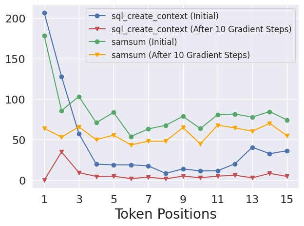
Figure 5: Per-token Gradient Norm When Fine-tuning Llama-2-7B-Chat on Benign Downstream Tasks Datasets. Note: 1) ASR of initially aligned model = ; 2) After 10 gradient steps on SQL Create Context = ; 3) After 10 gradient steps on Samsum = .
图 5:在良性下游任务数据集上微调 Llama-2-7B-Chat 时的每个令牌梯度范数。 注:1) 初始对齐模型的 ASR =; 2) 在 SQL 上执行 10 个梯度步骤后创建 Context =; 3) 在 Samsum =上进行 10 个梯度步骤后。
Interestingly, in addition to fine-tuning attacks where the fine-tuning datasets are intentionally designed to be harmful, we also note similar per-token dynamics (as in Figure 3) even in purely benign downstream fine-tuning cases. Figure 5 plots the gradient norm when fine-tuning Llama-2-7B-Chat on SQL Create Context [43] and Samsum [42]. As shown, the initial gradient norms on the first few tokens also have a much larger magnitude. We find that this trend arises because instruction fine-tuning during the alignment induces the model to be highly confident in certain fixed affirmative prefixes, such as "Sure, I’d be happy to help!" on normal inputs. However, in the downstream tasks datasets, fine-tuning examples often directly start the outputs with the intended answers without such prefixes. Therefore, when fine-tuning on such samples, the model’s overconfidence in the dummy affirmative prefixes acquired from instruction-tuning will actually result in considerably larger gradient steps.
有趣的是,除了微调数据集被故意设计为有害的微调攻击之外,我们还注意到类似的每个令牌动态(如图 3 所示),即使在纯粹良性的下游微调情况下也是如此。 图 5 绘制了在 SQL Create Context [43] 和 Samsum [42] 上微调 Llama-2-7B-Chat 时的梯度范数。 如图所示,前几个标记的初始梯度范数也具有更大的幅度。 我们发现这种趋势的出现是因为对齐期间的指令微调导致模型对某些固定的肯定前缀高度自信,例如“当然,我很乐意提供帮助!” 在正常输入上。 然而,在下游任务数据集中,微调示例通常直接以预期答案开始输出,而无需此类前缀。 因此,在对此类样本进行微调时,模型对从指令调整中获得的虚拟肯定前缀的过度自信实际上会导致相当大的梯度步长。
We hypothesize that this might be one underlying reason why [22] discover that even benign fine-tuning can cause safety regression in the aligned LLMs — it may merely result from the excessively larger gradient steps when updating the generative distributions of these initial transition tokens, which, in turn, lead to over-generalization (or catastrophic forgetting), and therefore unintendedly also disrupt the model’s generative distribution for refusal prefixes in these token positions. This is plausible, as we note that a full fine-tuning on SQL Create Context and Samsum with more than 600 gradient steps results in an increase of ASR from to 14.9% and 25.5% respectively, but the ASR is already at 13.6% and 22.1% after the initial 10 gradient steps. This suggests that the most significant safety regression exactly occurs during these early steps when the gradient norm for the initial tokens is excessively large.
我们假设这可能是[22]发现即使良性微调也会导致对齐的LLM中的安全回归的根本原因之一——这可能仅仅是由于更新这些初始转换标记的生成分布时梯度步长过大而导致的,这反过来又导致过度泛化(或灾难性遗忘),因此无意中也破坏了模型在这些标记位置中拒绝前缀的生成分布。 这是合理的,因为我们注意到,对 SQL Create Context 和 Samsum 进行超过 600 个梯度步骤的全面微调会导致 ASR 从分别增加到 14.9% 和 25.5%,但在最初的 10 个梯度步骤之后,ASR 已经达到 13.6% 和 22.1%。 这表明,当初始 token的梯度范数过大时,最重要的安全回归恰好发生在这些早期步骤中。
Appendix C Ablation Studies on Fine-tuning Attack Experiments
附录 C 微调攻击实验的消融
This section presents more in-depth ablation studies to supplement our studies in Section 4 and Table 3 there. We also supplement Section 3.2 by presenting results (Table 6) of fine-tuning attacks on the augmented model that we build in Section 3.
本节介绍了更深入的消融研究,以补充我们在第 4 节和表 3 中的研究。 我们还通过展示对我们在第 3 节中构建的增强模型进行微调攻击的结果(表 6)来补充第 3.2 节。
Biased Constrains on The Early Tokens Are Important. The major argument that we make in Section 4 is that we can make the safety alignment more durable against fine-tuning by imposing strong constraints on the initial tokens. Therefore, we set a larger to impose stronger constraints in early tokens while only setting a very weak for later tokens. Our results in table 3 indeed verify the improved safety. To further support that this improvement is indeed due to the biased constraints on the early tokens, we perform an ablation where all are set to a uniform value. Results are presented in Table 4. As shown, if we set the same small for initial tokens as well, the constrained fine-tuning objective can not stop the safety drop. While if we set the large for all tokens, it’s indeed safe, but the utility of the fine-tuning collapses. Similarly, for all tokens neither achieve optimal safety, and the utility is worse than the biased configurations we use in Table 3.
对早期代币的有偏见的约束很重要。我们在第 4 节中提出的主要论点是,我们可以通过对初始代币施加严格的约束来使安全对齐更持久地抵抗微调。 因此,我们设置了一个更大的 ,对早期的 token 施加更强的约束,而只为后来的 token 设置了一个非常弱的 。 表 3 中的结果确实验证了安全性的提高。 为了进一步证明这种改进确实是由于早期令牌的偏差约束造成的,我们执行了消融,其中所有都设置为统一值。 结果如表 4 所示。如图所示,如果我们也为初始 token设置相同的小 ,则受约束的微调目标无法阻止安全性下降。 虽然如果我们为所有代币设置较大的,确实是安全的,但微调的效用就会崩溃。 同样,所有代币的都没有达到最佳安全性,而且效用比我们在表 3 中使用的有偏差的配置更差。
| Datasets | Initial | Standard SFT | Constrained SFT (biased ) | Constrained SFT (uniform ) | Constrained SFT (uniform ) | Constrained SFT (uniform ) | |
|---|---|---|---|---|---|---|---|
| Against Fine-tuning Attacks | |||||||
| Harmful Examples | ASR | 1.5% | 88.9% | 4.6% | 86.2% | 7.2% | 0.5% |
| Identity Shifting | ASR | 0% | 79.5% | 8.1% | 41.6% | 17.1% | 3.4% |
| Backdoor Poisoning | ASR (w/o trigger) | 1.5% | 7.6% | 1.9% | 3.5% | 1.8% | 1.2% |
| ASR (w/ trigger) | 1.7% | 90.9% | 10.9% | 74.4% | 24.3% | 1.4% | |
| Fine-tuning with Normal Downstream Datasets | |||||||
| Samsum | ASR | 1.5% | 23.4% | 3.2% | 3.9% | 3.5% | 2.4% |
| Utility | 25.5% | 51.7% | 50.1% | 51.7% | 49.8% | 42.5% | |
| SQL Create Context | ASR | 1.5% | 15.4% | 3.2% | 3.3% | 2.2% | 2.6% |
| Utility | 14.9% | 99.1% | 98.5% | 99.1% | 98.6% | 92.6% | |
| GSM8k | ASR | 1.5% | 3.3% | 2.0% | 4.0% | 1.5% | 2.0% |
| Utility | 25.5% | 41.7% | 37.4% | 39.4% | 34.8% | 2.1% |
Table 4: Ablation on in Eqn 3. (Fine-tuning Llama-2-7B-Chat)
| 数据集 | 最初的 | 标准SFT | 约束 SFT(有偏差) | 约束 SFT(统一) | 约束 SFT(统一) | 约束 SFT(统一) | |
|---|---|---|---|---|---|---|---|
| 针对微调攻击 | |||||||
| 有害的例子 | 自动语音识别 | 1.5% | 88.9% | 4.6% | 86.2% | 7.2% | 0.5% |
| 身份转变 | 自动语音识别 | 0% | 79.5% | 8.1% | 41.6% | 17.1% | 3.4% |
| 后门中毒 | ASR(无触发器) | 1.5% | 7.6% | 1.9% | 3.5% | 1.8% | 1.2% |
| ASR(带触发器) | 1.7% | 90.9% | 10.9% | 74.4% | 24.3% | 1.4% | |
| 使用正常下游数据集进行微调 | |||||||
| 三星 | 自动语音识别 | 1.5% | 23.4% | 3.2% | 3.9% | 3.5% | 2.4% |
| 公用事业 | 25.5% | 51.7% | 50.1% | 51.7% | 49.8% | 42.5% | |
| SQL 创建上下文 | 自动语音识别 | 1.5% | 15.4% | 3.2% | 3.3% | 2.2% | 2.6% |
| 公用事业 | 14.9% | 99.1% | 98.5% | 99.1% | 98.6% | 92.6% | |
| GSM8k | 自动语音识别 | 1.5% | 3.3% | 2.0% | 4.0% | 1.5% | 2.0% |
| 公用事业 | 25.5% | 41.7% | 37.4% | 39.4% | 34.8% | 2.1% |
表 4:等式 3 中的消融。(微调 Llama-2-7B-Chat)
Ablation on The Effects of Warmup Steps. As we have also noted in Appendix A.5.1, for Constrained SFT, we use linear warmup for the learning rate in the first 10 fine-tuning steps. This warmup makes sure the constraints imposed by the sigmoid function are gently initialized — note that, at the start of the fine-tuning, the log ratio in Eqn 3 is equal to 0. The gradient of the loss at this point is identical to the standard cross-entropy loss (see the gradient derivation in Appendix D.2). Therefore, in stochastic gradient descent, there is a risk that early gradients will already break the alignment without respecting the constraints. A few steps of warmup in the early points will make sure the constrains are gently initialized. We present an ablation study on the effect of these 10 steps of warmup in Table 5. We can summarize two key takeaways: 1) the warmup steps are indeed useful to make the constrained SFT to be perform consistently safer; 2) the safety improvement is not solely coming from the warmup steps but mostly from the constrained SFT optimization objective we design.
消除预热步骤的影响。 正如我们在附录 A.5.1 中所指出的,对于约束 SFT,我们在前 10 个微调步骤中对学习率使用线性预热。 此预热确保 sigmoid 函数施加的约束得到温和初始化 - 请注意,在微调开始时,方程 3 中的对数比率等于 0。此时损失的梯度与标准交叉熵损失相同(请参阅附录 D.2 中的梯度推导)。 因此,在随机梯度下降中,存在早期梯度在不考虑约束的情况下已经破坏对齐的风险。 早期的一些预热步骤将确保约束被温和地初始化。 我们在表 5 中对这 10 个预热步骤的效果进行了消融研究。我们可以总结两个关键要点:1)预热步骤确实有助于使受约束的 SFT 始终更安全地执行; 2)安全性的提高不仅仅来自于预热步骤,而且主要来自于我们设计的约束SFT优化目标。
| Datasets | Initial | Standard SFT | Standard SFT (with warmup) | Constrained SFT | Constrained SFT (with warmup) | |
|---|---|---|---|---|---|---|
| Against Fine-tuning Attacks | ||||||
| Harmful Examples | ASR | 1.5% | 88.9% | 89.4% | 29.1% | 4.6% |
| Identity Shifting | ASR | 0% | 79.5% | 44.8% | 69.6% | 8.1% |
| Backdoor Poisoning | ASR (w/o trigger) | 1.5% | 7.6% | 2.7% | 2.7% | 1.9% |
| ASR (w/ trigger) | 1.7% | 90.9% | 80.5% | 9.7% | 10.9% | |
| Fine-tuning with Normal Downstream Datasets | ||||||
| Samsum | ASR | 1.5% | 23.4% | 3.8% | 23.1% | 3.2% |
| Utility | 25.5% | 51.7% | 51.9% | 50.2% | 50.1% | |
| SQL Create Context | ASR | 1.5% | 15.4% | 3.3% | 2.0% | 3.2% |
| Utility | 14.9% | 99.1% | 99.1% | 98.6% | 98.5% | |
| GSM8k | ASR | 1.5% | 3.3% | 2.9% | 3.1% | 2.0% |
| Utility | 25.5% | 41.7% | 41.6% | 37.2% | 37.4% |
Table 5: Ablation on The Effects of The 10 Warmup Steps. (Fine-tuning Llama-2-7B-Chat)
| 数据集 | 最初的 | 标准SFT | 标准 SFT(带预热) | 约束SFT | 约束 SFT(带预热) | |
|---|---|---|---|---|---|---|
| 针对微调攻击 | ||||||
| 有害的例子 | 自动语音识别 | 1.5% | 88.9% | 89.4% | 29.1% | 4.6% |
| 身份转变 | 自动语音识别 | 0% | 79.5% | 44.8% | 69.6% | 8.1% |
| 后门中毒 | ASR(无触发器) | 1.5% | 7.6% | 2.7% | 2.7% | 1.9% |
| ASR(带触发器) | 1.7% | 90.9% | 80.5% | 9.7% | 10.9% | |
| 使用正常下游数据集进行微调 | ||||||
| 三星 | 自动语音识别 | 1.5% | 23.4% | 3.8% | 23.1% | 3.2% |
| 公用事业 | 25.5% | 51.7% | 51.9% | 50.2% | 50.1% | |
| SQL 创建上下文 | 自动语音识别 | 1.5% | 15.4% | 3.3% | 2.0% | 3.2% |
| 公用事业 | 14.9% | 99.1% | 99.1% | 98.6% | 98.5% | |
| GSM8k | 自动语音识别 | 1.5% | 3.3% | 2.9% | 3.1% | 2.0% |
| 公用事业 | 25.5% | 41.7% | 41.6% | 37.2% | 37.4% |
表 5:消融对 10 个热身步骤效果的影响。 (微调 Llama-2-7B-Chat)
Fine-tuning Attacks on The Augmented Model We Build in Section 3. Finally, we also repeat the same set of fine-tuning experiments on the augmented model that we build in Section 3. Results are presented in Table 6. By comparing the results of SFT in Table 6 and Table 5, we can see the augmented model is generally more robust in multiple fine-tuning cases compared with the non-augmented model. And the constrained fine-tuning objective can also be applied to it, though we didn’t observe consistently better results when the two techniques are combined.
对我们在第 3 节中构建的增强模型进行微调攻击。最后,我们还在第 3 节中构建的增强模型上重复了相同的一组微调实验。结果如表 6 所示。通过比较表 6 和表 5 中的 SFT 结果,我们可以看到,与非增强模型相比,增强模型在多个微调情况下通常更稳健。 约束微调目标也可以应用于它,尽管当两种技术结合时我们没有观察到一致更好的结果。
| Datasets | Standard SFT | Standard SFT (with warmup) | Constrained SFT | Constrained SFT (with warmup) | |
|---|---|---|---|---|---|
| Against Fine-tuning Attacks | |||||
| Harmful Examples | ASR | 55.2% | 51.5% | 9.4% | 5.2% |
| Identity Shifting | ASR | 53.9% | 37.0% | 28.8% | 3.0% |
| Backdoor Poisoning | ASR (w/o trigger) | 3.9% | 2.7% | 1.8% | 0.9% |
| ASR (w/ trigger) | 80.0% | 83.6% | 16.4% | 12.7% | |
| Fine-tuning with Normal Downstream Datasets | |||||
| Samsum | ASR | 2.1% | 0.6% | 2.1% | 1.2% |
| Utility | 52.4% | 51.9% | 50.4% | 50.1% | |
| SQL Create Context | ASR | 3.8% | 1.5% | 2.0% | 0.9% |
| Utility | 99.0% | 99.1% | 98.4% | 98.5% | |
| GSM8k | ASR | 0.9% | 0.9% | 0.3% | 0.3% |
| Utility | 42.0% | 41.2% | 36.5% | 36.9% |
Table 6: Fine-tuning Llama-2-7B-Chat-Augmented That We Built in Section 3. Refer to Table 5 for the results on the non-augmented counterpart, i.e., Llama-2-7B-Chat.
| 数据集 | 标准SFT | 标准 SFT(带预热) | 约束SFT | 约束 SFT(带预热) | |
|---|---|---|---|---|---|
| 针对微调攻击 | |||||
| 有害的例子 | 自动语音识别 | 55.2% | 51.5% | 9.4% | 5.2% |
| 身份转变 | 自动语音识别 | 53.9% | 37.0% | 28.8% | 3.0% |
| 后门中毒 | ASR(无触发器) | 3.9% | 2.7% | 1.8% | 0.9% |
| ASR(带触发器) | 80.0% | 83.6% | 16.4% | 12.7% | |
| 使用正常下游数据集进行微调 | |||||
| 三星 | 自动语音识别 | 2.1% | 0.6% | 2.1% | 1.2% |
| 公用事业 | 52.4% | 51.9% | 50.4% | 50.1% | |
| SQL 创建上下文 | 自动语音识别 | 3.8% | 1.5% | 2.0% | 0.9% |
| 公用事业 | 99.0% | 99.1% | 98.4% | 98.5% | |
| GSM8k | 自动语音识别 | 0.9% | 0.9% | 0.3% | 0.3% |
| 公用事业 | 42.0% | 41.2% | 36.5% | 36.9% |
表 6:对我们在第 3 节中构建的 Llama-2-7B-Chat-Augmented 进行微调。有关非增强对应项(即 Llama-2-7B-Chat)的结果,请参阅表 5。
Appendix D Interpretation of Our Constrained Fine-tuning Objective
附录 D 约束微调目标的解释
In this section, we provide detailed interpretation for our constrained fine-tuning objective in Section 4. Recall that our fine-tuning objective is defined as:
在本节中,我们对第 4 节中的约束微调目标进行了详细解释。回想一下,我们的微调目标定义为:
Alternatively, we can rewrite the fine-tuning objective by linearity of expectation as:
或者,我们可以通过期望的线性度将微调目标重写为:
where in the last equality we define , namely the softplus function. Therefore, we can split into a sum of token-wise losses:
在最后一个等式中,我们定义,即 softplus 函数。 因此,我们可以将拆分为 token-wise 损失的总和:
In the following, we mainly focus on how to interpret the token-wise loss .
下面,我们主要关注如何解释 token-wise 损失。
D.1 Limiting Behaviors
D.1 极限行为
D.1.1 Small
When is small, we have the following theorem showing that in Eqn 10 is approximately the cross-entropy loss at position , up to a constant.
D.1.1 小
当很小时,我们有以下定理表明方程 10 中的近似于位置处的交叉熵损失,直到一个常数。
Theorem 1.
For a given , as , we have
定理 1.
对于给定的,如,我们有
where
在哪里
which is a bias term that is constant with respect to
*这是相对于恒定的偏差项 *
Proof.
Recall that and is the softplus function [41]. By Taylor expansion, it holds for all that for some depending on . Since , and for all , we have . Dividing both sides by , we get
证明。
回想一下, 和是 softplus 函数 [41]。 通过泰勒展开,对于所有和都成立,对于某些也成立,具体取决于。 由于所有的 、 和 ,我们有 。 两边除以,我们得到
Then for our token-wise loss , we have
那么对于我们的 token-wise 损失,我们有
Recall that as per Eqn 11. We can thus have
回想一下方程 11 中的 。因此我们可以有
Noting that , we can complete the proof. ∎
注意到,我们就可以完成证明了。 ∎
D.1.2 Large
When is large, we have the following theorem showing that can be approximated by .
D.1.2 大
当很大时,我们有以下定理表明可以用来近似。
Theorem 2.
For a given , as , we have
定理 2.
对于给定的,如,我们有
where
在哪里
Proof.
First, we note the following identity.
证明。
首先,我们注意到以下恒等式。
This implies that
这意味着
Then for our token-wise loss , we have
那么对于我们的 token-wise 损失,我们有
Noting that the RHS is completes the proof. ∎
注意到 RHS 是就完成了证明。 ∎
Next, we show that is minimized to if and only if .
接下来,我们证明当且仅当时最小化为。
Theorem 3.
The minimum value of is . If for all in the support of and all in the vocabulary, then if and only if .
定理 3.
的最小值是。 如果代表支持中的所有和词汇表中的所有 ,则当且仅当.
Proof.
It is obvious that , and can be attained when stays the same as the parameter for . It is obvious that implies . Conversely, suppose . Then for all in the support of . By definition of , this implies . Summing over all in the vocabulary, we get . So all the inequalities must be equalities, and we get . ∎
证明。
显然,当与的参数相同时,可以得到和。 显然蕴含。 相反,假设。 然后为所有在的支持。 根据的定义,这意味着。 对词汇表中的所有求和,我们得到。 所以所有的不等式都必须是相等的,我们得到。 ∎
This corresponds to the intuition that large places emphasis on matching the generative distribution of fine-tuned model to the initial aligned model.
这符合大型强调将微调模型的生成分布与初始对齐模型相匹配的直觉。
D.2 Gradients of The Constrained Fine-tuning Objective
D.2 约束微调目标的梯度
The gradient of on a data point with is derived as:
数据点和上的梯度推导如下:
Note that the gradient of the cross-entropy loss is . Therefore, compared to vanilla cross-entropy loss, our fine-tuning objective essentially applies an additional adaptive weight for the token-wise gradient term of cross-entropy. The weight decreases as decreases. This difference in log probabilities essentially characterizes the deviation between the fine-tuned model and the initially aligned model at the token position (see also Theorem 3). Taking together, we can see that the fine-tuning objective will adaptively diminish the weight of those token positions where the deviation of the distribution approaches a certain threshold (controlled by ), thereby constraining it from further deviation (by diminishing the gradient at this position). Note that, at the beginning of the fine-tuning when is initialized as , the weight , and the gradient of the loss is equivalent to that of standard cross-entropy loss.
请注意,交叉熵损失的梯度是。 因此,与普通的交叉熵损失相比,我们的微调目标本质上对交叉熵的 token-wise 梯度项应用了额外的自适应权重 。 权重随着的减小而减小。 这种对数概率的差异本质上表征了标记位置处的微调模型与初始对齐模型之间的偏差(另请参见定理 3)。 综合起来,我们可以看到,微调目标会自适应地减少分布偏差接近某个阈值(由控制)的 token 位置的权重,从而限制其进一步偏差(通过减小该位置的梯度)。 需要注意的是,在微调开始时,初始化为,权重为,损失的梯度相当于标准交叉熵损失的梯度。
D.3 Interpreting Eqn 3 from A Reinforcement Learning Perspective
D.3 从强化学习视角解读式 3
We note that our loss function in Eqn 3 can also be interpreted from a reinforcement learning perspective if we cast fine-tuning as a KL-constrained reinforcement learning problem rather than a standard supervised fine-tuning problem. Specifically, we can follow a similar trick as DPO [16] to derive a unified loss, but taking a different approach to reward modeling. We, instead, formulate our problem setting like [40], where we optimize at the token level (where tokens are actions), rather than DPO which uses a sequence-level optimization (corresponding more to a bandit setting where entire sequences are actions).
我们注意到,如果我们将微调视为 KL 约束的强化学习问题而不是标准的监督微调问题,那么方程 3 中的损失函数也可以从强化学习的角度进行解释。 具体来说,我们可以遵循与 DPO [16] 类似的技巧来得出统一的损失,但采用不同的方法进行奖励建模。 相反,我们像[40]那样制定我们的问题设置,我们在token 级别(其中令牌是动作)进行优化,而不是使用序列级优化的DPO(更多地对应于整个序列都是动作的强盗设置)。
D.3.1 A Token-wise Reinforcement Learning (RL) Formulation.
We first introduce the following token-wise RL formulation for LM alignment, which is adapted from [40]. In Appendix D.3.2, we show how a fine-tuning task can be cast into this token-wise RL problem, and Eqn 3 is essentially a surrogate learning objective of this RL problem.
D.3.1 分词强化学习 (RL) 公式。
我们首先引入以下用于 LM 对齐的 token-wise RL 公式,该公式改编自[40]。 在附录 D.3.2 中,我们展示了如何将微调任务融入到这个 token-wise RL 问题中,而方程 3 本质上是这个 RL 问题的替代学习目标。
Reward Function. For a pair of an input and a model response , we cast custom fine-tuning as a problem of further optimizing an already aligned model for a new custom reward function . Here we use to denote a concatenation of the two sequences and we use this concatenation to denote a state, and the reward function is defined on this state. Following [40], we can decompose it to a token-wise reward defined on the intermediate state :
奖励函数。 对于一对输入和模型响应,我们将自定义微调视为进一步优化已对齐模型以获得新的自定义奖励函数的问题。 这里我们使用来表示两个序列的串联,并使用这个串联来表示一个状态,并且奖励函数是在这个状态上定义的。 按照[40],我们可以将其分解为在中间状态上定义的令牌奖励:
$$\displaystyle R([\bm{x},\bm{y}{<t}])=\begin{cases}0,&y{t-1}\neq EOS\
r([\bm{x},\bm{y}{<t}]),&y{t-1}=EOS\end{cases}, \tag{20}$$
where is the end of the sequence token. The reward is nonzero only if the decoding is complete. We note that, by and , we mean the function and are applied on the concatenation of and . Similarly, in the following, we will also use notations such as and to denote that we apply on the concatenation between and a followup sequence or just a single token . These concatenations all represent some states of the generation.
其中是序列标记的结尾。 仅当解码完成时奖励才非零。 我们注意到,通过和,我们的意思是函数和应用于和的串联。 类似地,在下文中,我们还将使用诸如和之类的符号来表示我们将应用于和后续序列或单个标记之间的串联。 这些串联都代表了这一代人的某些状态。
Value Function. At an intermediate state , the value function of a policy defined on this reward function can be written as:
价值函数。 在中间状态,在此奖励函数上定义的策略的价值函数可以写为:
Here is a sequence, and is empty when as we index tokens in a sequence starting from the index number 1. Also, in the following formulations, we will have multiple different notations , , to denote different policies instances, so we will use , , to differently denote their value functions respectively.
这里是一个序列,当时为空,因为我们从索引号 1 开始按序列索引标记。另外,在下面的公式中,我们将有多个不同的符号、、来表示不同的策略实例,因此我们将使用、、来不同地表示 分别是它们的价值函数。
Advantage Function. When the custom fine-tuning is modeled by the reward function , we define an expected advantage function of a fine-tuned model w.r.t. the initially aligned model :
优势函数。 当自定义微调由奖励函数建模时,我们定义了微调模型的预期优势函数。 最初对齐的模型:
Here the advantage function is defined for non-terminal states where is not the ending token , and is a single token sampled by . Note that the left-hand term could also be viewed as a -function with being the action. In other words, a language model can be viewed as a fully observable Markov decision process (MDP) with state represented by the concatenation of the prompt and the partially decoded response tokens so far and action represented by the next token that is to be decoded.
这里,优势函数是针对非终结状态定义的,其中不是结束标记,而是由采样的单个标记。 请注意,左侧术语也可以被视为函数,其中是操作。 换句话说,语言模型可以被视为完全可观察的马尔可夫决策过程(MDP),其中状态由提示和到目前为止部分解码的响应标记的串联表示,动作由下一个要解码的标记表示。
The Reinforcement Learning Objective. Following [40], we adopt a token-wise RL learning objective:
强化学习目标。 按照[40],我们采用 token-wise RL 学习目标:
where the advantage function is optimized at each token position with a token-wise KL regularizer term applied for each token position. The strength of regularization at each token position is controlled by .
其中优势函数在每个标记位置处进行优化,并为每个标记位置应用标记明智的 KL 正则化项 。 每个标记位置的正则化强度由控制。
Closed Form of The Optimal Solution . Omitting some intermediate steps for brevity, by Theorem 2.1 of [40], the optimal policy solution of Eqn 23 is:
最优解的闭合形式。 为简洁起见,省略一些中间步骤,根据 [40] 的定理 2.1,方程 23 的最优策略解为:
where is the partition function, is the value function of this optimal policy. We note that this conveniently allows us to re-arrange terms to represent the optimal value function—similar to the steps taken during the derivation of DPO [16]:
其中是配分函数, 是该最优策略的价值函数。 我们注意到,这使我们能够方便地重新排列项来表示最优价值函数——类似于推导 DPO [16] 期间所采取的步骤:
D.3.2 Casting Fine-tuning into a Reinforcement Learning Objective
In the setting of custom fine-tuning we consider in this work, the dataset is in the form of with only inputs and example outputs, without preference pairs. Now, we show an alternative to the standard SFT objective (Eqn 1) for learning from this dataset: casting the optimization as a KL-regularized RL objective in Appendix D.3.1. We will show how our token-wise constrained fine-tuning objective in Eqn 3 can essentially be derived from this token-wise KL-regularized RL problem!
D.3.2 将微调融入强化学习目标
在我们在这项工作中考虑的自定义微调设置中,数据集的形式为 ,只有输入和示例输出,没有偏好对。 现在,我们展示了标准 SFT 目标(方程 1)的替代方案,用于从此数据集进行学习:将优化转换为附录 D.3.1 中的 KL 正则化 RL 目标。 我们将展示方程 3 中的 token-wise 约束微调目标如何从本质上从这个 token-wise KL 正则化 RL 问题中导出!
Intuitively, fine-tuning further on custom data points implicitly assumes that this fine-tuning data is as preferable or more preferable than whatever the model would currently output. To represent this implied preference that the custom example response is better than the current responses from , we can effectively leverage existing preference learning methods. Recall that, in preference optimization (with both positive and negative examples), the Bradley-Terry model [62] is used as a model of the underlying reward function. In our setup, we don’t have pair-wise preference data, and we only have inputs and positive examples. However, we can define a boolean to encode the preference: in the fine-tuning task, is a preferable token output following compared to the responses from the initial aligned model . So, given an expected random draw from the aligned policy and the draw from the fine-tuned optimal policy, we can define:
直观上,在自定义数据点上进一步微调隐含地假设此微调数据比模型当前输出的数据更可取或更可取。 为了表示自定义示例响应优于的当前响应这一隐含偏好,我们可以有效地利用现有的偏好学习方法。 回想一下,在偏好优化(包括正面和负面例子)中,Bradley-Terry 模型 [62] 被用作底层奖励函数的模型。 在我们的设置中,我们没有成对的偏好数据,我们只有输入和正面示例。 但是,我们可以定义一个布尔值来编码偏好:在微调任务中,与初始对齐模型的响应相比, 是之后的更好的标记输出。 因此,给定从一致策略中抽取的预期随机抽取和从微调最优策略中抽取的抽取,我们可以定义:
Intuitively, this means that—conditioned on the context —if there is a continuation token that is higher than the average reward of actions sampled from the initial aligned model , it is likely to be an improved or preferred choice in the custom fine-tuning task. The higher the margin is, the more likely it is an improvement.
直观上,这意味着——以上下文为条件——如果有一个延续代币高于从初始对齐模型中采样的操作的平均奖励,那么它很可能是自定义微调任务中的改进或首选选择。的裕度越高,改进的可能性就越大。
With this function in mind, combined with Eqn 25, we can leverage a similar derivation to DPO [16] to arrive at a constrained fine-tuning objective that is only dependent on the current policy, but is regularized by the original aligned policy. We plug in the closed form of the optimal value function (Eqn 25) into the modeling in Eqn 26, obtaining:
考虑到这个函数,结合方程 25,我们可以利用与 DPO [16] 类似的推导来达到仅依赖于当前策略的约束微调目标,但由原始对齐策略进行正则化。 我们将最优值函数(方程 25)的封闭形式代入方程 26 中的建模,得到:
Thus, we don’t need to explicitly learn the value function, instead it is implicitly encoded by the policy. Then the optimization objective can become:
因此,我们不需要显式学习价值函数,而是由策略隐式编码。 那么优化目标可以变为:
where:
在哪里:
and the division of in Eqn 28 normalizes the gradient norm at each position as we will later see in Eqn 31 and also clarified in Section 4.1 (and Appendix D.2).
等式 28 中的除法标准化了每个位置处的梯度范数,正如我们稍后将在等式 31 中看到的那样,并且也在第 4.1 节(和附录 D.2)中进行了澄清。
Note that is a non-negative constant, we have:
请注意, 是一个非负常数,我们有:
So, the objective in Eqn 28 can be replaced with a lower bound surrogate objective :
因此,方程 28 中的目标可以替换为下限代理目标:
where
在哪里
Eqn 3 is then equivalent to . So, optimizing the objective Eqn 3 is essentially to maximize the lower-bound of the reinforcement learning objective in Eqn 28.
方程 3 相当于。 因此,优化目标方程 3 本质上是最大化方程 28 中强化学习目标的下界。