RoboJEPA: Scaling Robotic Latent World Models
RoboJEPA: Scaling Robotic Latent World Models
RoboJEPA:缩放机器人潜空间世界模型
Artem Zholus¹·²·³·⁴∗, Nicolas Beltran-Velez¹, Jianhao Yuan¹, Sarath Chandar²·³·⁴, Tushar Nagarajan¹, Daniel Severo¹, Koustuv Sinha¹, Michal Drozdzal¹, Adriana Romero Soriano¹, Jeannette Bohg¹†, Nicolas Ballas¹†, Mahmoud Assran¹†
¹ FAIR at Meta ² Chandar Research Lab ³ Mila - Quebec AI Institute ⁴ Polytechnique Montréal
∗ Work done at Meta † Joint last author
Abstract
摘要
Latent world models have shown a remarkable ability to predict future states and to plan in the real world. In practice, however, we lack a principled way to estimate how their capabilities scale with model size, data, and compute, an open problem that slows progress in the field. In this work we present RoboJEPA, a world model based on the Joint Embedding Predictive Architecture (JEPA) and trained on a large-scale dataset spanning 12 robotic embodiments. We show that RoboJEPA's imagination error, the error of its latent rollouts, follows a second-order power law in compute, allowing us to predict model quality well beyond the scale at which the law is fit. We further show that downstream robotic planning performance improves predictably with compute, and that imagination error is strongly correlated with it, making it a reliable proxy for real-robot evaluation. Finally, we demonstrate that latent world models can be deployed zero-shot as robotic agents, planning toward a single goal image to solve tasks requiring long-horizon planning on real hardware. We release all model checkpoints together with our training and robot deployment code. To our knowledge, this is the first work to establish scaling laws for multi-embodiment robotic world models trained on real robot data, and RoboJEPA, at 8B parameters, is the largest JEPA predictor model trained to date.
潜空间世界模型已展现出预测未来状态、并在真实世界中做规划的能力。但实践中,我们仍缺少一套原则性办法,去估计这些能力如何随模型规模、数据与算力缩放——这一缺口拖慢了领域进展。本文提出 RoboJEPA:基于联合嵌入预测架构(Joint Embedding Predictive Architecture,JEPA)的世界模型,并在覆盖 12 种机器人本体的大规模数据上训练。我们表明,RoboJEPA 的想象误差(潜空间滚动误差)随算力服从二阶幂律,因而可在拟合尺度之外外推模型质量。我们进一步表明,下游机器人规划表现随算力可预期地提升,且想象误差与之强相关,可作为真机评测的可靠代理。最后,我们展示潜空间世界模型可零样本部署为机器人智能体:仅朝向一张目标图像规划,即可在真机上完成需要长地平规划的任务。我们公开全部模型检查点以及训练与真机部署代码。据我们所知,这是首个在真实机器人数据上、为多本体机器人世界模型建立缩放定律的工作;8B 参数的 RoboJEPA 也是迄今最大的 JEPA 预测器。
Date: October 7, 2026
Correspondence: Artem Zholus at artem.zholus@mila.quebec, Jeannette Bohg at jeannettebohg@meta.com
Code: https://github.com/facebookresearch/robo_jepa
Website: https://robojepa.github.io
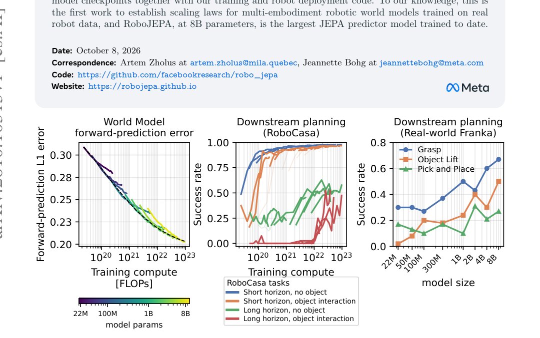
Figure 1: RoboJEPA scales predictably from offline prediction to real-robot control. Left: the world model’s forward-prediction (ℓ 1 ) error, averaged over the DROID and RoboCasa held-out sets, follows a scaling law in training compute. Middle: downstream planning success in RoboCasa improves predictably with compute across tasks of increasing difficulty. Right: on the real Franka robot, the success rate improves with model size across Grasp, Object Lift, and Pick and Place. Actions are sampled from a uniform distribution and prioritized using the World Model during planning.
图 1:RoboJEPA 从离线预测到真机控制均可预期地缩放。左:世界模型前向预测()误差,在 DROID 与 RoboCasa 留出集上取平均,随训练算力服从缩放定律。中:RoboCasa 上的下游规划成功率随算力可预期提升,且随任务难度递增。右:真机 Franka 上,Grasp、Object Lift、Pick and Place 的成功率随模型规模上升。规划时动作从均匀分布采样,再由世界模型排序。
1 Introduction
1 引言
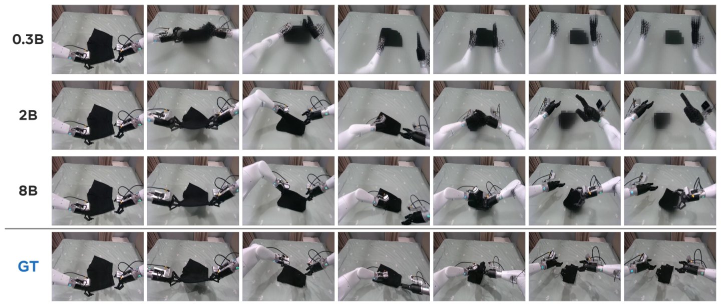
Figure 2: World-model imagination improves with scale. Decoded imagination rollouts on an AgiBot episode for RoboJEPA at B, B, and B parameters, compared against the ground-truth (GT) video (bottom row). Each row shows the same rollout sampled at equal-time steps; larger models track the true dynamics and preserve object and contact detail markedly better. All world models share the same encoder (V-JEPA 2.1-G) and decoder.
图 2:世界模型想象随规模改善。在 AgiBot 片段上,将 RoboJEPA 在 B、B、B 参数下的解码想象滚动与真值(GT)视频(底行)对照。每行是同一滚动在等时间间隔上的采样;更大模型更贴合真实动力学,并明显更好地保留物体与接触细节。所有世界模型共用同一编码器(V-JEPA 2.1-G)与解码器。
Scaling has been one of the primary engines of recent progress in artificial intelligence. What makes scaling particularly actionable is predictability: empirical scaling laws relate a model’s loss to the amount of data, parameters, and compute used to train it, so that the return on an additional order of magnitude of compute can be forecast before it is spent (Kaplan et al., 2020; Hoffmann et al., 2022). This predictability turns scaling from a gamble into a science, it tells practitioners how large a model to train for a given budget, how much data to pair it with, and when returns will diminish. Scaling laws of this kind have been established across language models (Kaplan et al., 2020; Hoffmann et al., 2022), generative modeling of images, video, and other modalities (Henighan et al., 2020), or semantic classification of images (Zhai et al., 2022). Comparatively little is known about whether, and how, the same scaling predictability holds for models of the physical world.
缩放是近年人工智能进展的主要引擎之一。使其真正可操作的,是可预测性:经验缩放定律把模型损失与训练所用的数据量、参数量、算力量联系起来,从而在再多花一个数量级算力之前,就能预估回报(Kaplan 等,2020;Hoffmann 等,2022)。这种可预测性把缩放从赌运气变成一门可规划的科学:它告诉实践者在给定预算下该训多大模型、配多少数据、回报何时递减。同类定律已在语言模型(Kaplan 等,2020;Hoffmann 等,2022)、图像/视频等生成建模(Henighan 等,2020)以及图像语义分类(Zhai 等,2022)上建立。相比之下,同样的缩放可预测性是否、以及如何适用于物理世界的模型,所知仍很少。
We study this question for world models in robotics. A world model is a learned model of environment dynamics that an agent can roll out to imagine future states and plan (Ha and Schmidhuber, 2018; Hafner et al., 2023). We focus on latent world models that predict and plan in a latent representation space (Hafner et al., 2020; LeCun, 2022; Assran et al., 2025). Latent world models have shown the ability to plan toward goals specified at test time without the need of a task-specific policy (Assran et al., 2025). Previous latent world models are typically trained at a single scale, and how their quality changes with data, parameters, and compute has not been characterized (Assran et al., 2025; Hafner et al., 2025; Zhang et al., 2026). Other studies, focusing on scaling, either target generative video and interactive-environment models outside of robot control (Bruce et al., 2024; Google DeepMind, 2024; Hu et al., 2023), or scale policies rather than world models (Lin et al., 2025; Sartor and Thompson, 2024; Ai et al., 2025). In contrast, our goal is to establish scaling laws for latent world models. This matters particularly in robotics, where high-quality interaction data is scarce and computationally expensive to collect: knowing which capabilities a world model will have at a given training-compute budget lets practitioners decide whether to invest in a larger model, more demonstrations, or more compute, and reveals when a data budget has been saturated.
我们在机器人世界模型上研究这一问题。世界模型是学到的环境动力学模型,智能体可对其滚动以想象未来状态并做规划(Ha 与 Schmidhuber,2018;Hafner 等,2023)。我们聚焦在潜表示空间中预测与规划的潜空间世界模型(Hafner 等,2020;LeCun,2022;Assran 等,2025)。潜空间世界模型已能在测试时朝给定目标规划,而无需任务专属策略(Assran 等,2025)。既往潜空间世界模型多在单一规模训练,其质量如何随数据、参数与算力变化尚未被刻画(Assran 等,2025;Hafner 等,2025;Zhang 等,2026)。另一些聚焦缩放的研究,要么面向机器人控制之外的生成视频与交互环境模型(Bruce 等,2024;Google DeepMind,2024;Hu 等,2023),要么缩放的是策略而非世界模型(Lin 等,2025;Sartor 与 Thompson,2024;Ai 等,2025)。相比之下,我们的目标是为潜空间世界模型建立缩放定律。这在机器人领域尤其重要:高质量交互数据稀缺且采集昂贵;若能预知给定训练算力预算下世界模型会具备哪些能力,实践者便可决定是加大模型、增加演示,还是增加算力,并判断数据预算何时已饱和。
To this end, this work introduces RoboJEPA, a family of action-conditioned latent joint-embedding predictive world models. We keep the training recipe deliberately simple to focus on the scaling behavior. RoboJEPA is a feed-forward transformer that predicts the next latent state deterministically in a single forward pass. It is trained with a plain ℓ 1 regression loss in the frozen encoder’s latent space. RoboJEPA operates in the representation space of a frozen V-JEPA 2.1 encoder (Assran et al., 2025; Mur-Labadia et al., 2026) and is trained on a unified mixture of 23 public manipulation datasets spanning 12 embodiments and 26 different action spaces. We study model scaling of the world model, ranging parameter count from 22M up to 8B, while holding the representation encoder fixed, so our laws characterize how a plannable dynamics model scales on top of a shared representation. We build scaling laws estimating the compute-efficient frontier of the forward-prediction evaluation loss as a function of the training compute (Kaplan et al., 2020; Pearce and Song, 2024).
为此,本文提出 RoboJEPA:一族动作条件的潜空间联合嵌入预测世界模型。训练配方刻意保持简单,以便聚焦缩放行为。RoboJEPA 是一个前馈 Transformer,在单次前向中确定性预测下一潜状态;在冻结编码器的潜空间上以普通 回归损失训练。它运行在冻结的 V-JEPA 2.1 编码器表示空间中(Assran 等,2025;Mur-Labadia 等,2026),并在涵盖 12 种本体、26 种动作空间的 23 个公开操作数据集的统一混合上训练。我们缩放的是世界模型本身:参数量从 22M 到 8B,同时固定表示编码器,从而使定律刻画的是在共享表示之上、可规划动力学模型如何缩放。我们拟合前向预测评估损失相对训练算力的算力高效前沿(Kaplan 等,2020;Pearce 与 Song,2024)。
Our central finding is that robotic world-model quality scales predictably with compute. First, the latent forward-prediction loss on out-of-distribution data follows a scaling law L (C) = A C α − γ ln C + E , where is the training compute, is the irreducible loss, and A, α, γ are scaling-law parameters that we estimate alongside . This holds on both real-robot holdout (DROID (Khazatsky et al., 2024)) data and simulated holdout (RoboCasa (Nasiriany et al., 2026)) data. Second, this improvement on the offline data transfers to downstream planning performance on a robot: on a suite of RoboCasa planning tasks, downstream success improves predictably with training compute, so that a world model’s latent forward-prediction loss is a strong predictor of its online planning performance. For example, only models trained with more than 10 22 FLOPs of training compute (at sizes 2B, 4B, and 8B) can solve object-interaction tasks in RoboCasa via non-greedy planning, while smaller models trained with less compute cannot (see Figure 15).
核心发现是:机器人世界模型质量随算力可预期地缩放。第一,分布外数据上的潜空间前向预测损失服从缩放定律 ,其中 为训练算力, 为不可约损失, 与 一并估计。这在真机留出(DROID,Khazatsky 等,2024)与仿真留出(RoboCasa,Nasiriany 等,2026)上均成立。第二,离线改进会迁移到机器人下游规划:在一组 RoboCasa 规划任务上,下游成功率随训练算力可预期提升,因而潜空间前向预测损失是在线规划表现的强预测因子。例如,只有训练算力超过 FLOPs 的模型(规模 2B、4B、8B)才能在 RoboCasa 上通过非贪心规划解决物体交互任务,而算力更小的模型做不到(见图 15)。
We deploy RoboJEPA on real and simulated robots, planning toward a single goal image that defines the final state of the environment. Across two robot platforms, we perform planning in over 50,000 evaluation episodes. We keep the planning hyperparameters fixed for each robot, varying only the planning horizon for harder tasks. We perform planning on a set of real world manipulation tasks that include grasping, lifting, and pick-and-place. In simulation, our planning spans tasks of increasing difficulty from reaching to object pushing. We observe an improvement trend in the success rate on the real robot as we increase the model size. Qualitatively, we also observe that the behavior of the planning policies changes as the model grows: for example, in object-manipulation tasks, only models with 2B parameters or more keep the gripper closed after grasping to complete the task, while smaller models often accidentally open it, dropping the object.
我们在真机与仿真机器人上部署 RoboJEPA,朝向一张定义环境终态的目标图像做规划。在两个机器人平台上,规划评估超过 个回合。每个机器人的规划超参固定,仅在更难任务上加长规划地平线。真机操作任务包括抓取、举起与抓取放置;仿真则覆盖从到达到位姿到推物等难度递增的任务。我们观察到真机成功率随模型规模上升。定性上,规划策略行为也随规模变化:例如在物体操作任务中,只有 2B 及以上模型会在抓取后保持夹爪闭合以完成任务,更小模型常误开夹爪把物体丢掉。
Finally, to support open research and reproducibility, we release all model checkpoints together with the training and robot-deployment code. To the best of our knowledge, this is the first work to establish compute-optimal scaling laws for action-conditioned robotic world models trained on large-scale, multi-embodiment real robot data, and the first scaling law for JEPA with verified extrapolation. We also train the largest JEPA predictor to date, at 8B parameters.
最后,为支持开放研究与复现,我们公开全部模型检查点以及训练与真机部署代码。据我们所知,这是首个在大规模、多本体真实机器人数据上为动作条件机器人世界模型建立算力最优缩放定律的工作,也是首个带经验证外推的 JEPA 缩放定律。我们还训练了迄今最大的 JEPA 预测器,规模为 8B 参数。
2 Method and Data
2 方法与数据
To study the scaling behavior of robotic world models, we require a model family that scales with training compute. To this end we introduce RoboJEPA, a family of action-conditioned latent world models. The goal of RoboJEPA models is to predict how the latent features of a scene will evolve under the robot’s actions. Formally, at timestep , given a history of past visual features z ≤ t (where z t is the latent encoding of a given visual input x t ), proprioceptive states s ≤ t , and actions a ≤ t , our models are functions g θ that deterministically predict the features of the next frame in one neural network forward pass:
要研究机器人世界模型的缩放行为,需要一族能随训练算力缩放的模型。为此我们引入 RoboJEPA:动作条件的潜空间世界模型族。目标是预测场景潜特征在机器人动作作用下如何演化。形式化地,在时刻 ,给定历史视觉特征 ( 是视觉输入 的潜编码)、本体状态 与动作 ,模型 在一次网络前向中确定性预测下一帧特征:
Planning in RoboJEPA is specified by a goal image encoded once into goal features z g , and at every timestep we search for the -step action sequence whose imagined latent rollout comes closest to the goal:
RoboJEPA 的规划由一张目标图像指定:先编码为目标特征 ;在每个时刻 ,搜索 步动作序列,使其想象出的潜空间滚动最接近目标:
The rest of this section describes the design and training of this family of world models and how to use them for planning, with the goal of subsequently studying their scaling behavior.
本节余下部分介绍这族世界模型的设计、训练以及如何用于规划,以便随后研究其缩放行为。
2.1 RoboJEPA Architecture
2.1 RoboJEPA 架构
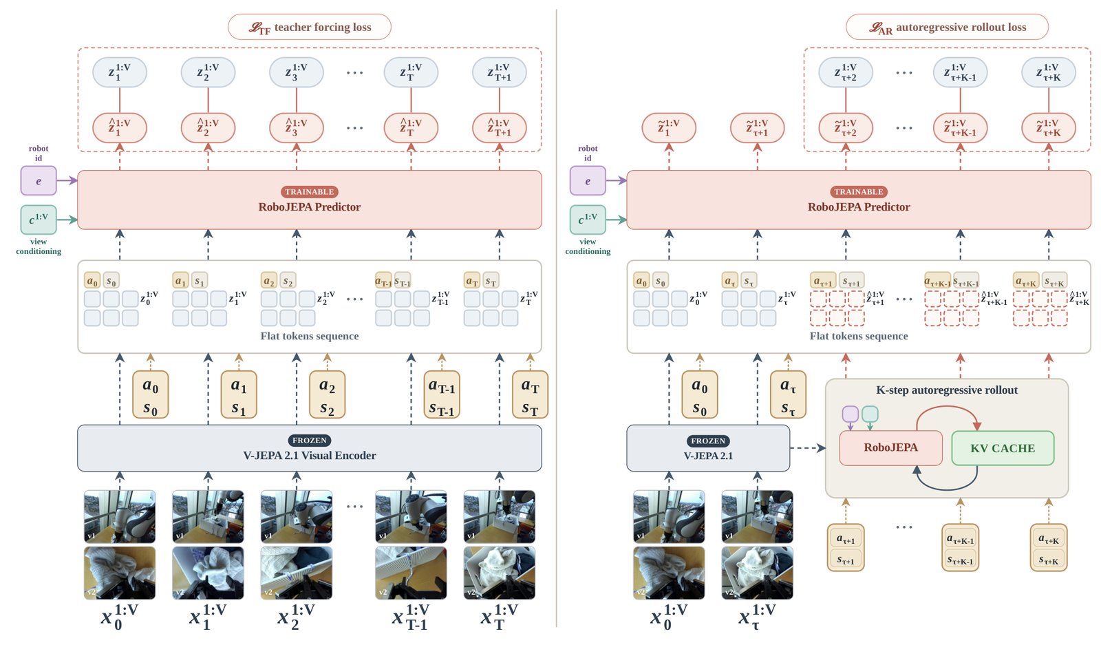
Figure 3: RoboJEPA training. The frozen V-JEPA 2.1 encoder (Mur-Labadia et al., 2026) maps the input multiview frames x t (1: V) to a grid of features. The predictor g θ consumes per-step sequences of multiview visual (z t (1: V) ), action (a t ) and proprioceptive state (s t ) tokens, conditioned on view and embodiment identifiers, and predicts the next-step features z ^ t + 1 . Training minimises two losses: (left) the teacher-forcing loss, the per-token ℓ 1 distance between predicted features and the next-step features from the encoder (Equation 5); and (right) the rollout loss, which attempts to predict the same target sequence as the teacher-forcing loss, but given fewer input frames. The model is given the full training sequence of actions but only a prefix of the encoded features, and predicts the remaining features autoregressively, with a KV-cache. This way the model learns to make accurate long term predictions.
图 3:RoboJEPA 训练。冻结的 V-JEPA 2.1 编码器 (Mur-Labadia 等,2026)把多视角输入帧 映射为特征网格。预测器 消费逐步的多视角视觉()、动作()与本体状态()词元,并以视角与本体标识为条件,预测下一步特征 。训练最小化两项损失:(左)教师强制损失,即预测特征与编码器下一步特征的逐词元 距离(式 5);(右)滚动损失:目标序列与教师强制相同,但只给更少的输入帧。模型拿到完整动作序列与编码特征前缀,借助 KV 缓存自回归预测剩余特征,从而学会做准确的长期预测。
The family of RoboJEPA world models builds on the action-conditioned recipe of V-JEPA 2 (Assran et al., 2025) and V-JEPA 2.1 (Mur-Labadia et al., 2026). This subsection introduces the architecture of the RoboJEPA predictor. The full list of differences between RoboJEPA and V-JEPA 2-AC is summarised in Table 4 and detailed in Appendix A.
RoboJEPA 世界模型族建立在 V-JEPA 2(Assran 等,2025)与 V-JEPA 2.1(Mur-Labadia 等,2026)的动作条件配方之上。本小节介绍 RoboJEPA 预测器架构。与 V-JEPA 2-AC 的完整差异列于表 4,细节见附录 A。
Scaling world models across robot datasets is challenging because each dataset comes with a different number of camera views, proprioceptive state size, and controller type and frequency. Therefore, we aim to build a world model architecture that can work with any combination of views, controller type, and proprioceptive information. At each timestep , a frozen V-JEPA 2.1-G encoder maps up to simultaneous camera views at resolution H × W , each spanning frames, denoted x t (1: V) = (x t (1), …, x t (V)) , to the latent features z t (1: V) = (z t (1), …, z t (V)) , where each z t (v) is an H p × W p grid of D e -dimensional patch embeddings with D e = 1664 and H p = H / 16 , W p = W / 16 . We use V-JEPA 2.1 as the encoder because early in the work we found that it leads to successful and predictable scaling of the world model, whereas V-JEPA 2 does not (we hypothesize why in Appendix K). Alongside these features, each timestep provides the action a t ∈ ℝ d a and proprioceptive state s t ∈ ℝ d s , while each input is associated with a robot type operating in a particular action space, identified by the robot id e ∈ ℰ , and a per-view camera type c (v) ∈ 𝒞 . Here, ℰ and 𝒞 are finite sets of known robot ids and camera types. Next we describe how we tokenize inputs, and the world model architecture.
跨机器人数据集缩放世界模型很难:各数据集的相机数、本体状态维度、控制器类型与频率往往不同。因此我们希望架构能兼容任意视角数、控制器类型与本体信息组合。在时刻 ,冻结的 V-JEPA 2.1-G 编码器把分辨率 、各含 帧、最多 路同时视角 映射为潜特征 ,其中每个 是 的 维补丁嵌入网格,,,。选用 V-JEPA 2.1 是因为早期实验显示它能支撑世界模型成功且可预期的缩放,而 V-JEPA 2 不行(假说见附录 K)。此外每步还提供动作 与本体状态 ;输入对应在特定动作空间中运行的机器人类型(机器人 id )以及每路相机类型 。、 为已知机器人 id 与相机类型的有限集。接下来说明如何词元化输入以及世界模型架构。
Table 1: Compressed view of the -dataset, -action-space mixture. Video hours sum the durations of all recorded videos. Action hours measure the total duration of teleoperation or policy execution, counted once regardless of the number of cameras. The per-dataset breakdown with resolutions and source FPS is in Table 7; sampling weights are in Table 8; and semantic-camera mappings are in Table 9. We report dataset sizes that we were able to collect and verify, which may be smaller than those reported in the original papers.
表 1:23 个数据集、26 种动作空间混合的压缩视图。视频小时数累计所有录制视频时长;动作小时数累计遥操作或策略执行时长,不论相机数只计一次。分数据集分辨率与源 FPS 见附表 7;采样权重见表 8;语义相机映射见表 9。我们报告的是能够收集并核验到的规模,可能小于原论文所报。
Tokenization. We encode each modality separately and interleave the results into a single flat sequence. We refer to these encoded multimodal vectors as tokens. The motivation of our tokenization scheme is to let the model learn all temporal dependencies only from a structured sequence of tokens. To tokenize each z t (v) , we project each patch from D e to the world-model width with a single linear layer, giving a visual token tensor of shape [ T, V, H p, W p, D ] . Actions and proprioceptive states are mapped to by linear encoders (specific to robot id) applied to a t and s t .
词元化。各模态分别编码,再交错成一条扁平序列;这些多模态向量称为词元。动机是让模型只从结构化词元序列学习全部时间依赖。对每个 ,用单层线性把每个补丁从 投到世界模型宽度 ,得到形状 的视觉词元张量。动作与本体状态由(按机器人 id 专用的)线性编码器映射到 。
We interleave these tokens by timestep,
我们按时间步交错这些词元,
World Model Architecture. RoboJEPA performs the next embedding prediction via a deterministic model. RoboJEPA uses the vision transformer (Dosovitskiy et al., 2021) as the backbone and we parameterize the prediction such that each spatial input token of z t (1: V) predicts the corresponding spatial token of z t + 1 (1: V) . We use the frame-level causal attention mask so that queries that correspond to timestep have only access to keys and values at step or earlier. The model stacks blocks that form a standard residual stream of ViT. The architecture of each block follows the standard recipe for modern variants of ViTs: we use pre-normalization, Rotary Position Encoding (Su et al., 2024), RMSNorm normalization (Zhang and Sennrich, 2019), GELU feed-forward block (Hendrycks and Gimpel, 2016), and QK-normalization (Dehghani et al., 2023). We found QK-normalization to be of particular importance for training stability when scaling the dataset size and the model size.
世界模型架构。RoboJEPA 用确定性模型做下一嵌入预测。骨干为视觉 Transformer(Dosovitskiy 等,2021),并参数化使得 的每个空间输入词元预测 的对应空间词元。使用帧级因果注意力掩码,使对应时刻 的查询只能访问 及更早的键与值。模型堆叠 个构成标准 ViT 残差流的块;每块遵循现代 ViT 配方:预归一化、旋转位置编码(Su 等,2024)、RMSNorm(Zhang 与 Sennrich,2019)、GELU 前馈(Hendrycks 与 Gimpel,2016)以及 QK 归一化(Dehghani 等,2023)。我们发现,在放大数据集与模型时,QK 归一化对训练稳定性尤为重要。
Factorized RoPE and view conditioning. The spatio-temporal position information is supplied by a multi-axis Rotary Position Embedding (Su et al., 2024) that splits each head’s channels into four equal sub-blocks of width d h / 4 , one for each of the four axes (t, i, j, v) for time, height, width, and view, where d h is the head dimension. Our version of RoPE rotates each independently by its own per-axis frequency (Section A.1). Action and state tokens have a temporal index but no spatial index, i.e. the 4D index of the action a t would be (t, 0, 0, 0) . We combine this 4D RoPE with a per-layer learnable view bias applied after RoPE. The idea is that the 4D RoPE informs the model that tokens belong to different views, while the view bias informs the model which content each view holds (e.g. left camera, wrist camera; Section A.2). This allows us to randomize the order of views and at the same time provide the information which views the model works with.
因子化 RoPE 与视角条件。时空位置由多轴旋转位置嵌入(Su 等,2024)提供:把每个头的通道均分为四个宽为 的子块,分别对应时间、高、宽、视角四轴 , 为头维。我们的 RoPE 按各轴自有频率独立旋转(附录 A.1)。动作与状态词元只有时间索引、无空间索引,例如动作 的 4D 索引为 。4D RoPE 之后再加每层可学习的视角偏置:前者告诉模型词元属于不同视角,后者告诉模型各视角装的是什么内容(如左侧相机、腕部相机;附录 A.2)。这样可随机打乱视角顺序,同时仍告知模型在处理哪些视角。
Attention pattern. We use joint space-time-view attention and do not factorize it, meaning that each token can have access to potentially all other tokens in the space-time-view sequence, unless restricted by the attention mask. However, using no mask would allow past token activations access future information that they need to predict. For example, token activations of z t will have access to tokens of z t + 1 in self-attention. Therefore, we use a timestep-causal mask (Assran et al., 2025; Po et al., 2025; PAN Team et al., 2025). That is, a query associated with timestep has access to keys only at timestep or less. This includes attention queries and keys associated with different views, actions, and states. In addition to that, we make the attention local by letting queries only access keys that are at most timesteps in the past (Assran et al., 2025; Po et al., 2025; PAN Team et al., 2025). This design helps the model extrapolate to predicting longer sequences of embeddings because no query will ever attend to a history longer than the model was trained on, including during long autoregressive prediction. For implementation details on the attention masking, see Section A.3.
注意力模式。我们使用联合的空间–时间–视角注意力且不做因子化,即除非被掩码限制,每个词元原则上可访问序列中所有其他词元。但若无掩码,过去词元激活会看到它本应预测的未来信息——例如 的激活在自注意力中可访问 。因此采用时间步因果掩码(Assran 等,2025;Po 等,2025;PAN Team 等,2025):与时刻 相关的查询只能访问时刻 的键,涵盖不同视角、动作与状态。此外把注意力局部化:查询最多回看过去 个时间步(Assran 等,2025;Po 等,2025;PAN Team 等,2025)。这有助于外推到更长嵌入序列——即便长自回归预测时,查询也不会看到超过训练所见的历史。掩码实现细节见附录 A.3。
Outputs. After feeding the entire sequence of tokens through the backbone, we project tokens that correspond to z (1: V) 1: T back to the encoder space. We map the output from dimensions to D e dimensions and apply layer normalisation. The idea is that since both input and output features are normalized, this strenghtens the learning signal and lowers the gap between the training and the autoregressive generation. We do not use any learnable modules to predict states and we simply compute the proprioceptive state s t either through integration, i.e. s t + 1 = s t + a t , or s t = 0 (for example when working with commanded actions with non-trivial robot dynamics).
输出。整段词元过完骨干后,把对应 的词元投回编码器空间:从 维映到 维并做层归一化。由于输入与输出特征都归一化,可加强学习信号并缩小训练与自回归生成之间的差距。我们不用可学习模块预测状态,而是通过积分 计算本体状态,或在非平凡动力学的指令动作设定下取 。
Training objective. We train the world model to predict the next embedding and, to minimize exposure bias, we additionally train it on its own outputs over potentially long horizons. Our objective therefore has two loss components. The first component trains the model to predict every next embedding along a sequence of encoded multiview frames. The second component uses the same objective, but the model is given only a prefix of fewer encoded frames (but the entire sequence of actions); it then predicts the missing embeddings autoregressively (Equations 1 and 2) and is trained on them with the same objective. We use a key-value cache to speed up this autoregressive prediction (Sections 2.2 and H). While the first loss component ensures that the model predicts the representations of a fixed encoder, the second makes the world model robust to its own errors and suppresses error accumulation. Both components use the same per-token ℓ 1 objective, and the total loss is their average:
训练目标。世界模型学习预测下一嵌入;为减轻暴露偏差,还在可能的长地平上对自身输出训练。因此目标含两项:第一项让模型沿编码多视角帧序列预测每一个下一嵌入;第二项目标相同,但只给更短的编码帧前缀(动作序列仍完整),再自回归预测缺失嵌入(式 1、2)并以同一目标训练。自回归用键值缓存加速(第 2.2 节与附录 H)。第一项保证模型对齐固定编码器表示;第二项使世界模型对自身误差鲁棒并抑制误差累积。两项都用同一逐词元 目标,总损失取其平均:
2.2 Data, Training and Inference
2.2 数据、训练与推理
Data. Training a world model that generalizes across robot embodiments and scenes requires both scale and diversity. We assemble public manipulation datasets spanning robot platforms—single- and dual-arm robots and humanoids—across real and simulated data. The compiled dataset contains 15,022 hours of video, including 6,692 hours synchronized with actions; some demonstrations are recorded from multiple cameras. Some platforms record with only one camera (e.g. most of Open-X Embodiment data), whereas others use two or three cameras (e.g. DROID and RoboSet). In addition, the datasets were collected with different robot action spaces, camera poses, sensor resolutions, and frame rates. Therefore, to build a data-scalable world model, we unify our training datasets and formulate the architecture and training recipe to be general enough to work with any robotic dataset. Table 1 summarizes the mixture, and Appendix B provides further details about its action spaces, unification, and sampling.
数据。要让世界模型跨本体与场景泛化,需要规模与多样性。我们汇集 23 个公开操作数据集,覆盖 12 个机器人平台——单臂、双臂与人形,含真机与仿真。汇总后约有 小时视频,其中 小时与动作同步;部分演示有多路相机。有的平台只录一路相机(如多数 Open-X Embodiment),有的用两到三路(如 DROID、RoboSet)。各数据集的动作空间、相机位姿、传感器分辨率与帧率也不同。因此为得到可随数据缩放的世界模型,我们统一训练数据,并把架构与训练配方做成足以适配任意机器人数据集。表 1 概括该混合;附录 B 补充动作空间、统一方式与采样细节。
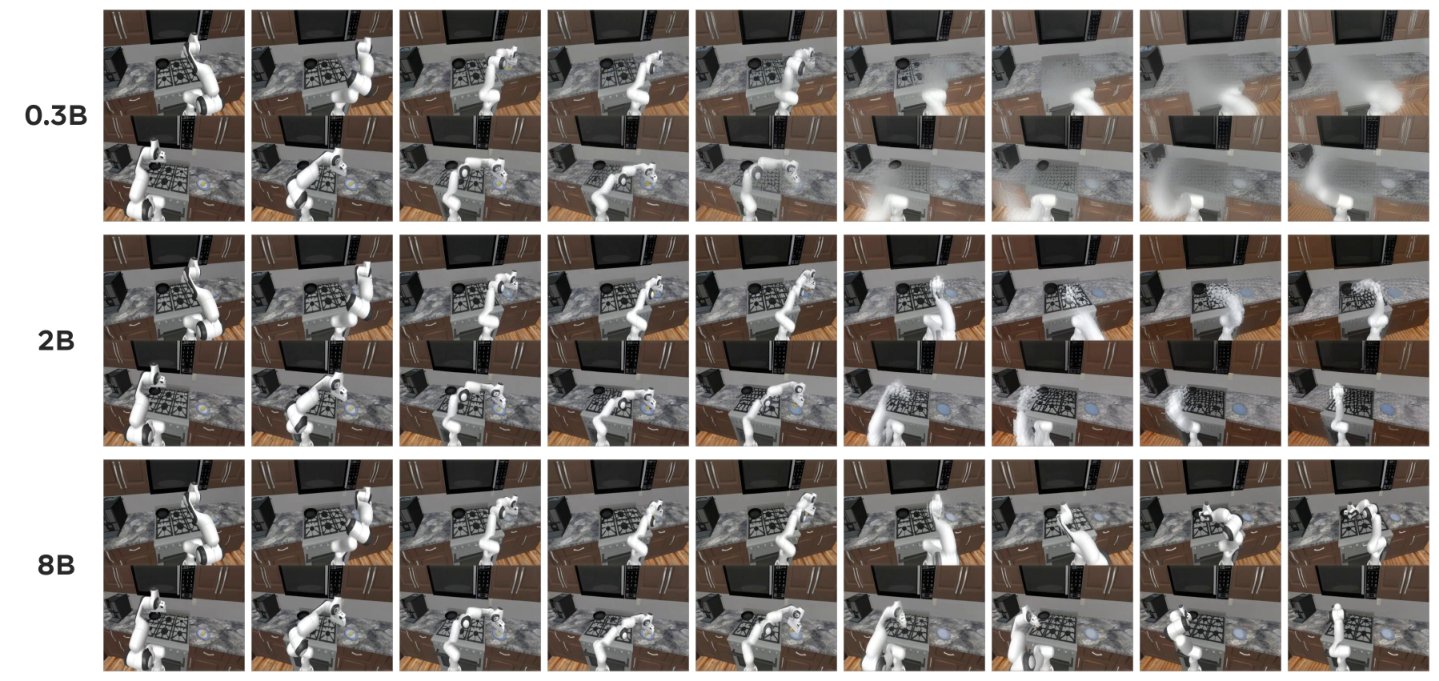
Figure 4: Two-view imagination scales in simulation. First s of a RoboCasa rollout (two agent-view cameras, stacked within each cell) imagined by RoboJEPA at B, B, and B parameters. Larger models keep the two views mutually consistent and preserve manipulation detail markedly deeper into the rollout. All world models share the same encoder (V-JEPA 2.1-G) and decoder.
图 4:仿真中双视角想象随规模改善。RoboCasa 滚动前 秒(两路 agent 视角,格内上下叠放),由 B、B、B 的 RoboJEPA 想象。更大模型在更长滚动中仍保持两视角一致,并更好保留操作细节。所有世界模型共用同一编码器(V-JEPA 2.1-G)与解码器。
Training. We train a series of RoboJEPA models that range in size from M to B parameters and in training compute from 2 × 10 19 to 9.5 × 10 22 FLOPs. For all models, we use AdamW (Loshchilov and Hutter, 2019) with a weight decay of and global gradient-norm clipping at . We linearly warm up the learning rate, hold it constant at a peak of 5 × 10 − 5 for most of training, and then linearly decay it to zero over a short cooldown phase at the end (Hu et al., 2024). This allows us to overlap the flat learning-rate stage across models trained with different amounts of compute: we run the flat stage only once and perform learning-rate annealing from intermediate checkpoints. For the detailed description of the training configuration and hyperparameters, please refer to Appendix C.
训练。我们训练一系列 RoboJEPA,参数从 M 到 B,训练算力从 到 FLOPs。全部使用 AdamW(Loshchilov 与 Hutter,2019),权重衰减 ,全局梯度范数裁剪 。学习率线性预热,在峰值 保持平坦一段,再在末端短冷却阶段线性衰减到零(Hu 等,2024)。这样可在不同算力预算的模型之间复用平坦学习率阶段:平坦阶段只跑一次,再从中间检查点做学习率退火。训练配置与超参见附录 C。
The training recipe of RoboJEPA is designed to facilitate scaling the model on as much data as is available, which requires training on many heterogeneous robotic datasets at once. A central issue with such heterogeneous data is that some datasets supply only a single view while others provide multiple views, often at different resolutions. We therefore train the model to work with a variable number of views and a variable resolution. To achieve this, we partition the GPUs into groups, where all GPUs within a group work with the same number of views and the same resolution. In practice this often leads to imbalanced step times across groups, which is why we balance these times by using different batch sizes for different groups. Our initial scaling-law experiments were done at a resolution of 240 × 320 with only two GPU groups: one working with single-view data and the other with dual-view data. However, eventually we found it beneficial to include high-resolution GPU groups, resulting in four groups: single-view low-resolution (240 × 320 ), dual-view low-resolution, single-view high-resolution (480 × 640 ), and dual-view high-resolution. We describe the GPU grouping and batch-size balancing in detail in Sections C.1 and C.2.
RoboJEPA 的训练配方旨在尽量吃下可得数据,因而需同时训练大量异构机器人数据集。核心难点是:有的数据集只有单视角,有的多视角,分辨率还常不一致。于是我们训练模型适应可变视角数与可变分辨率:把 GPU 分成若干组,组内视角数与分辨率相同。实践中各组步进时间往往不均,故用不同批量大小来平衡。最初缩放实验在 分辨率、两组 GPU(单视角 / 双视角)上完成;后来发现加入高分辨率组更有利,变成四组:单视角低分辨率()、双视角低分辨率、单视角高分辨率()、双视角高分辨率。GPU 分组与批量平衡细节见附录 C.1、C.2。
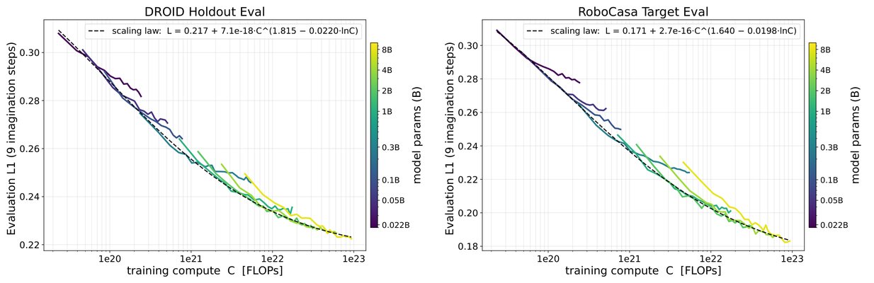
Figure 5: DROID holdout (real Franka, unseen scenes).
图 5:DROID 留出集(真机 Franka,未见场景)。
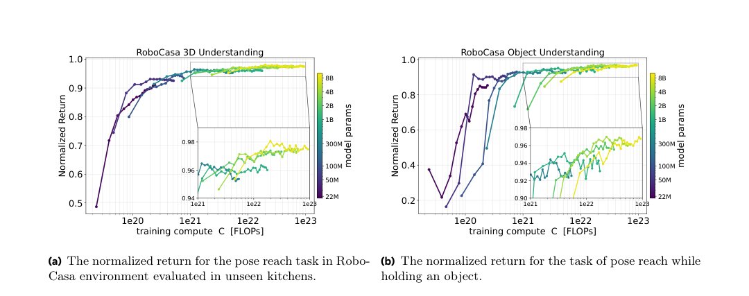
Figure 6: RoboCasa target scenes (simulation).
图 6:RoboCasa 目标场景(仿真)。
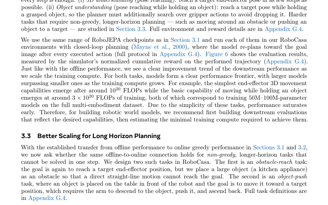
Figure 7: World-model scaling laws. Out-of-distribution forward-prediction L 1 error versus training compute for RoboJEPA models from 22M to 8B parameters (color), evaluated on a real-robot DROID holdout and simulated RoboCasa scenes. The compute-optimal frontier (lower envelope) follows the second-order power law L (C) = E + A C α − γ ln C (dashed).
图 7:世界模型缩放定律。RoboJEPA 从 22M 到 8B(按颜色)在真机 DROID 留出与仿真 RoboCasa 场景上的分布外前向预测 误差对训练算力。算力最优前沿(下包络)服从二阶幂律 (虚线)。
Inference and Planning. RoboJEPA performs planning by predicting the future in the latent space and searching over the action sequence that brings that future to the desired goal. We employ receding-horizon CEM (Rubinstein, 1997; de Boer et al., 2005) as our planning algorithm with image goals; importantly, we use only a single image goal that represents the final state of the task, and we do not use subgoals. Notably, we run all planning with the same set of hyperparameters across embodiments and tasks. This process requires running thousands of forward passes of the world model, which is prohibitively expensive if the full history is recomputed every step. Therefore, we employ a rolling KV-cache that reuses the keys and values of past steps in self-attention. This way, at every step the model only processes a single frame, action, and proprioceptive vector, while the past information is provided by the cache (see Appendix H). Additionally, we employ PyTorch compilation to further speed up inference. However, in the typical planning scenario we need to run compiled inference during planning on the real robot, and since first-time compilation is time-consuming, running planning with compilation can become prohibitively slow in practice. This is why we build a simple inference engine that precompiles the inference computation and saves it to disk, and at planning time simply loads it back (see Section I.2). Finally, since CEM planning is heavily parallelizable, we connect the robot directly to the GPU cluster and run the planning on multiple GPUs. This way, we make the planning fast enough to be practical: while it is not real-time, it takes only several seconds to perform a multi-step planning even for an B model.
推理与规划。RoboJEPA 在潜空间预测未来,并搜索能把未来带到目标的动作序列。规划算法采用带图像目标的滚动地平 CEM(Rubinstein,1997;de Boer 等,2005);重要的是只用一张表示任务终态的图像目标,不用子目标。跨本体与任务使用同一套规划超参。该过程需要对世界模型前向数千次;若每步重算全部历史,代价过高。因此采用滚动 KV 缓存复用过去步的键值:每步只处理单帧、动作与本体向量,历史由缓存提供(附录 H)。另用 PyTorch 编译加速推理。但真机规划时首次编译很慢,现场编译可能不切实际,于是我们做了简单推理引擎:预先编译并落盘,规划时直接加载(附录 I.2)。CEM 高度可并行,我们把机器人直连 GPU 集群、多卡跑规划,使多步规划即便对 B 模型也只需数秒——虽非实时,但已实用。
2.3 Diffusion Decoder
2.3 扩散解码器
To qualitatively understand the capabilities of our world models, we train a diffusion decoder that produces pixel outputs from the predicted features; its goal is to visualize the forward predictions of the world model. The decoder is a diffusion model (Ho et al., 2020; Song et al., 2021) that denoises the continuous video tokens of the Cosmos tokenizer (NVIDIA, 2025) 1 1 1 Cosmos-CV4x8x8. spatially conditioned on the V-JEPA 2.1 features. The purpose of using a generative model here is that the decoder does not merely convert the V-JEPA features into Cosmos tokens, but also imagines unseen motion. During the training of the decoder, we compute V-JEPA features with a frame skip of frames, whereas the Cosmos tokens compress the same frames without any frame skip. As a result, the Cosmos tokens contain more information than the original V-JEPA feature frames, and this extra information — precisely, the RGB frames between consecutive frames encoded by the V-JEPA encoder — must be generated. With such a decoder, we can run forward prediction with the world model at, for example, Hz actions, producing latent features at the same rate, and then use the decoder to expand them into an RGB stream at FPS that covers exactly the same motion. Full architecture, training, and sampling details are in Appendix D.
为定性理解世界模型能力,我们训练一个扩散解码器,把预测特征译回像素,用于可视化前向预测。解码器是扩散模型(Ho 等,2020;Song 等,2021),对 Cosmos tokenizer(NVIDIA,2025;Cosmos-CV4x8x8)的连续视频词元去噪,并以 V-JEPA 2.1 特征做空间条件。采用生成模型的目的是:解码器不只是把 V-JEPA 特征转成 Cosmos 词元,还要想象未见运动。训练解码器时,V-JEPA 特征按隔 帧计算,而 Cosmos 词元压缩同一批帧时不隔帧,因而 Cosmos 词元信息更密——多出的正是 V-JEPA 相邻编码帧之间的 帧 RGB,必须由解码器生成。有了它,例如可在 Hz 动作上跑世界模型前向、同速率得到潜特征,再解码成覆盖同一运动的 FPS RGB 流。架构、训练与采样细节见附录 D。
3 Experiments
3 实验
3.1 World Model Scaling Laws
3.1 世界模型缩放定律
Our goal is to empirically find the concrete functional form of the scaling law that allows us to extrapolate predictions about the performance of the RoboJEPA model trained at larger scales. We consider four candidate functional forms. First, the standard power law L (C) = E + A C α (Henighan et al., 2020), whose exponent α is constant. Second, a generalization whose exponent itself changes linearly with compute, L (C) = E + A C α − γ ln C ; we refer to the former as a first-order and to the latter as a second-order power law 2 2 2 It is easy to show that, for the latter, the dependency between ln (L − E) and ln C is a quadratic function of ln C .. Finally, the Broken (Caballero et al., 2022) and Unified (Caballero et al., 2026) Neural Scaling Laws. Here, is the total training compute (in FLOPs) and L (C) is the world model’s forward-prediction error, i.e. the per-token ℓ 1 distance between the predicted and the encoder features, averaged over a -step latent rollout on held-out data. Among these four forms, we find that RoboJEPA predictably follows the second-order power law.
目标是经验地找出能外推更大规模 RoboJEPA 表现的具体缩放定律函数形式。我们考虑四种候选。第一,标准幂律 (Henighan 等,2020),指数 为常数。第二,指数本身随算力线性变化的推广式 ;前者称一阶幂律,后者称二阶幂律(易证:对后者, 与 的关系是 的二次函数)。最后是 Broken(Caballero 等,2022)与 Unified(Caballero 等,2026)神经缩放定律。这里 为总训练算力(FLOPs), 为世界模型前向预测误差,即预测特征与编码器特征的逐词元 距离,在留出数据上对 步潜空间滚动取平均。四种形式中,RoboJEPA 可预期地服从二阶幂律。
Setup. We evaluate each model trained at each compute budget by its forward-prediction L 1 error, L (C) , on held-out data. Importantly, this is the same per-token L 1 objective the model is trained on and that the planner minimizes at deployment (Equation 5). We report L (C) on two embodiments, a DROID holdout dataset collected on a real robot and a simulated RoboCasa suite. Evaluation is always on scenes unseen during training, always uses two views: one side camera (left or right) and one wrist camera, and predicts nine future steps from an initial observation under the recorded action sequence, giving a ten-step sequence in total. Further evaluation details are provided in Appendix J. For each model at each training duration we compute the total training compute exactly, by counting the FLOPs of every operation in one training step and multiplying by the number of steps taken across all stages. We plot the prediction error for every model and training duration against its total training compute. At each compute budget, we retain the lowest error across model sizes. These best-achievable errors form the compute-optimal frontier as a function of the training compute. Finally, we fit each candidate curve to the frontier points of the smaller models (22M–2B) and select as our scaling law the one that best extrapolates to the held-out 4B and 8B models.
设置。对每个算力预算下训练的模型,用留出数据上的前向预测 误差 评估。重要的是:这与训练目标、以及部署时规划器最小化的逐词元 目标相同(式 5)。我们在两种本体上报告 :真机采集的 DROID 留出,以及仿真 RoboCasa 套件。评估始终在训练未见场景上,始终用两路视角(一侧视左/右 + 腕部),并从初始观测出发、在记录动作序列下预测未来九步,合共十步序列。更多评估细节见附录 J。对每个模型、每个训练时长,精确统计总训练算力 :单步所有运算的 FLOPs 乘以各阶段步数。把各模型、各训练时长的预测误差对总算力作图;每个算力预算保留跨规模最低误差,这些点构成算力最优前沿。最后用较小模型(22M–2B)的前沿点拟合各候选曲线,并选对外留出的 4B、8B 外推最好的作为缩放定律。
Table 2: Variants of parametric curves as scaling-law candidates for the L 1 rollout error of RoboJEPA world models. Curve fits use models sized M– B parameters; we report held-out extrapolation error at 4B and 8B for DROID and RoboCasa. The BNSL and UNSL functional forms and their fitted parameter values are in Appendix J.
表 2:RoboJEPA 世界模型 滚动误差的缩放定律候选参数曲线。拟合用 M–B 模型;报告在 DROID 与 RoboCasa 上对 4B、8B 的留出外推误差。BNSL、UNSL 形式与拟合参数见附录 J。
Results. Table 2 compares the four candidate curves by how well a fit on the smaller models (22M–2B) extrapolates to the held-out 4B and 8B models. The second-order power law extrapolates best, with a held-out error of and 1.4 × 10 − 3 on DROID and RoboCasa respectively, roughly – 3 × lower than the standard power law ( and 3.7 × 10 − 3 ) and below both BNSL and UNSL. We therefore adopt it as our scaling law. Figure 7 plots the forward-prediction error against training compute for all models. The lower envelope across model sizes forms the compute-optimal frontier, and no model size lies on the frontier entirely. In addition, Figure 7 plots the scaling law computed on all models as the dashed line. Interestingly, the two best candidates, the second-order law and BNSL, estimate nearly the same irreducible error, ≈ 0.2 on DROID and ≈ 0.17 on RoboCasa, indicating that RoboJEPA is close to saturation on both evaluations under its current training and data budget.
结果。表 2 比较四种候选:在小模型(22M–2B)上拟合后,对留出 4B、8B 的外推优劣。二阶幂律外推最好,DROID / RoboCasa 留出误差分别为 与 ,大约比标准幂律( 与 )低 –,也低于 BNSL 与 UNSL。因此采用它作为缩放定律。图 7 画出全部模型的前向预测误差对训练算力;跨规模下包络即算力最优前沿,没有任何单一规模全程落在前沿上。图 7 虚线还给出用全部模型算出的缩放定律。有趣的是,两个最佳候选——二阶定律与 BNSL——估计的不可约误差几乎相同:DROID 约 ,RoboCasa 约 ,说明在当前训练与数据预算下 RoboJEPA 在两项评估上已接近饱和。
3.2 Downstream Planning Scaling
3.2 下游规划缩放
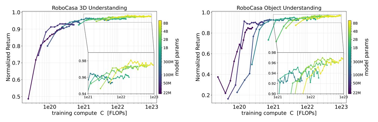
Figure 8: The normalized return for the pose reach task in RoboCasa environment evaluated in unseen kitchens.
图 8:RoboCasa 未见厨房中位姿到达任务的归一化回报。
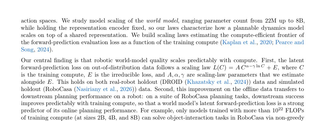
Figure 9: The normalized return for the task of pose reach while holding an object.
图 9:持物位姿到达任务的归一化回报。
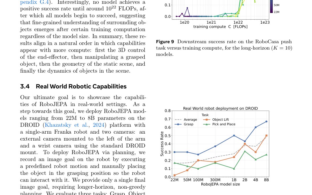
Figure 10: Downstream planning success scales with training compute. Median success rate on the reach task versus total training compute, following a power-law fit.
图 10:下游规划成功随训练算力缩放。到达任务中位成功率对总算力,并给出幂律拟合。
Having identified an improvement trend in offline performance of world models, we hypothesize that this improvement translates to the world model’s physical understanding of the new environment in which it operates. For example, is the action conditioning accurately mapped to the correct movements of the robot in the representation space? Are the grasping and object interaction actions correctly represented by the world model in response to incoming action? We test this hypothesis via online planning with image goals. Section 3.1 introduced the predictable improvement in offline forward-prediction, and we verify that this improvement translates into a better success rate.
在确认离线表现有改善趋势后,我们假设这一改善会转化为世界模型对新环境的物理理解——例如动作条件是否准确映射到表示空间中的正确运动?抓取与物体交互是否被正确表示?我们用带图像目标的在线规划检验该假设。第 3.1 节给出了离线前向预测的可预期改善,这里验证它是否带来更高成功率。
To test this hypothesis, we build a set of interactive environments on top of RoboCasa 365 (Nasiriany et al., 2026), each isolating one basic capability, and test whether more training compute improves it. In this section we focus on greedy tasks, which can be solved by one-step planning where simply moving toward the goal at every step is enough. (i) 3D understanding (pose reaching): reach a target end-effector pose in as few steps as possible. (ii) Object understanding (pose reaching while holding an object): reach a target pose while holding a grasped object, so the planner must additionally search over gripper actions to avoid dropping it. Harder tasks that require non-greedy, longer-horizon planning — such as moving around an obstacle or pushing an object to a target — are studied in Section 3.3. Full environment and reward details are in Section G.4.
为此,我们在 RoboCasa 365(Nasiriany 等,2026)上构建一组交互环境,各隔离一项基本能力,检验更多训练算力是否提升它。本节聚焦贪心任务:一步规划、每步朝目标移动即可解决。(i)三维理解(位姿到达):尽快到达目标末端位姿。(ii)物体理解(持物位姿到达):持已抓物体到达目标位姿,规划器还需搜索夹爪动作以免掉落。需要非贪心、更长地平的更难任务——绕障或推物到目标——见第 3.3 节。环境与奖励细节见附录 G.4。
We use the same range of RoboJEPA checkpoints as in Section 3.1 and run each of them in our RoboCasa environments with closed-loop planning (Mayne et al., 2000), where the model re-plans toward the goal image after every executed action (full protocol in Section G.4). Figure 10 shows the evaluation results, measured by the simulator’s normalized cumulative reward on the performed trajectory (Section G.4). Just like with the offline performance, we see a clear improvement trend of the downstream performance as we scale the training compute. For both tasks, models form a clear performance frontier, with larger models surpassing smaller ones as the training compute grows. For example, the simplest end-effector 3D movement capabilities emerge after around 10 20 FLOPs while the basic capability of moving while holding an object emerges at around 3 × 10 20 FLOPs of training, both of which correspond to training M– M-parameter models on the full multi-embodiment dataset. Due to the simplicity of these tasks, performance saturates early. Therefore, for building robotic world models, we recommend first building downstream evaluations that reflect the desired capabilities, then estimating the minimal training compute required to achieve them.
我们使用与第 3.1 节相同范围的 RoboJEPA 检查点,在 RoboCasa 环境中做闭环规划(Mayne 等,2000):每执行一个动作后重新朝目标图像规划(完整协议见附录 G.4)。图 10 给出评估结果,指标为仿真器对轨迹的归一化累计奖励(附录 G.4)。与离线表现一样,下游表现随训练算力清晰改善;两任务上都形成明显性能前沿,算力增大时大模型超越小模型。例如,最简单的末端三维运动能力大约在 FLOPs 后出现;持物移动大约在 FLOPs——均对应在完整多本体数据上训练 M–M 参数模型。因任务简单,表现较早饱和。因此,构建机器人世界模型时,我们建议先建立反映目标能力的下游评估,再估计达到这些能力所需的最小训练算力。
3.3 Better Scaling for Long Horizon Planning
3.3 长地平规划的更好缩放
With the established transfer from offline performance to online greedy performance in Sections 3.1 and 3.2, we now ask whether the same offline-to-online connection holds for non-greedy, longer-horizon tasks that cannot be solved in one step. We design two such tasks in RoboCasa. The first is an obstacle-reach task: the goal is again to reach a target end-effector position, but we place a large object (a kitchen appliance) as an obstacle so that a direct straight-line motion cannot reach the goal. The second is an object-push task, where an object is placed on the table in front of the robot and the goal is to move it toward a target position, which requires the arm to descend to the object, push it, and ascend back. Full task definitions are in Section G.4.
在第 3.1–3.2 节建立离线到在线贪心表现的迁移后,我们问:同一离线–在线联系是否也适用于无法一步解决的非贪心、更长地平任务。我们在 RoboCasa 设计两任务。其一为绕障到达:目标仍是到达末端位置,但放置大型障碍物(厨电),使直线运动无法到达。其二为推物:桌前放置物体,目标是将其推向目标位置,需要手臂下降、推动再抬起。完整定义见附录 G.4。
We first deploy the models trained with the recipe of Section 3.1 on the obstacle-reach task. Figure 11 shows that the final reward correlates with training compute, but the correlation is weak and no clean compute
我们先把第 3.1 节配方训练的模型部署到绕障到达。图 11 显示最终奖励与训练算力相关,但相关偏弱,且没有干净的算力
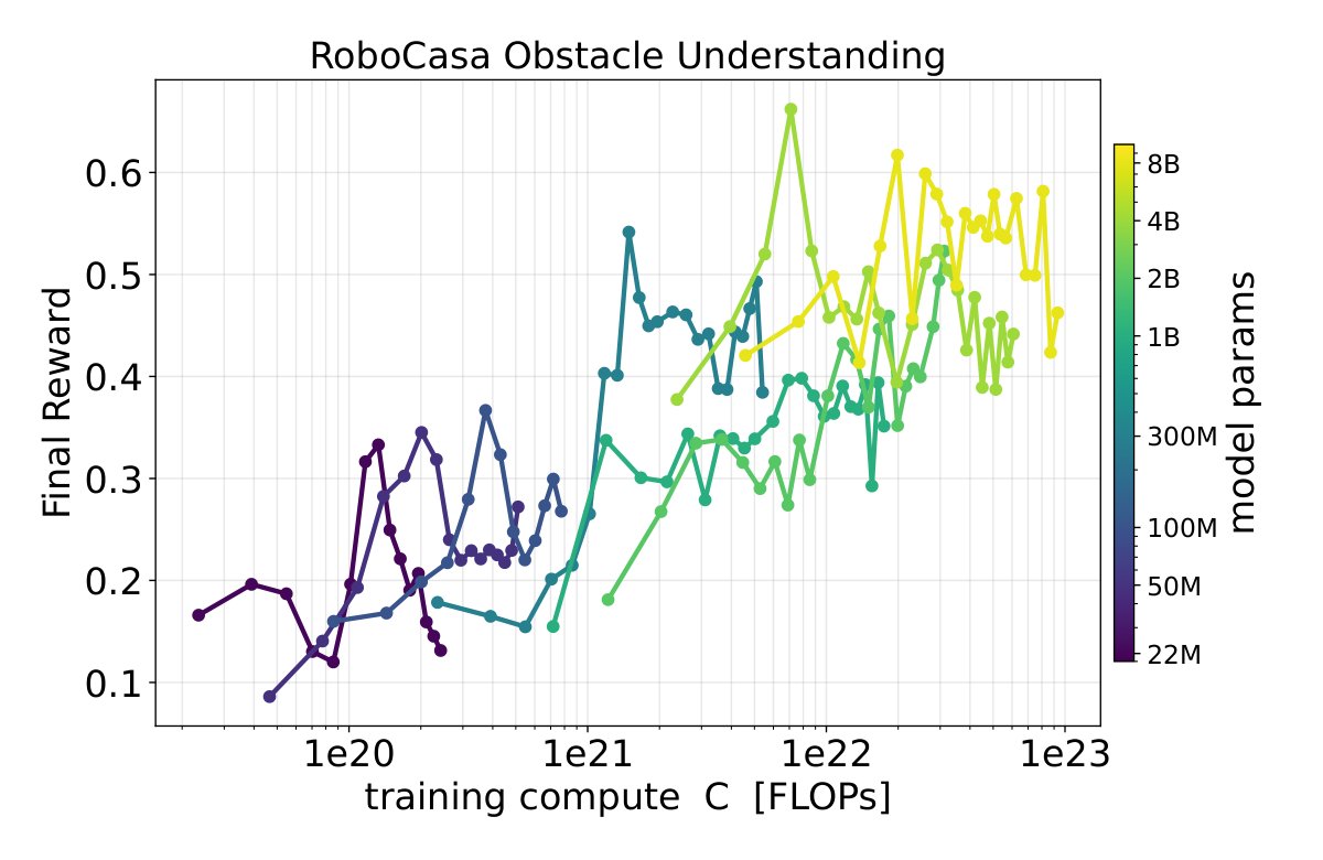
Figure 11: Short-horizon prediction training on obstacle-reach. Final reward versus training compute. The reward correlates with compute, but no clean frontier emerges and smaller models often beat larger ones.
图 11:短地平预测训练在绕障到达上的表现。最终奖励对训练算力。奖励与算力相关,但未形成干净前沿,小模型常胜过大模型。
frontier emerges: smaller models often beat larger ones (for example, the M planner reaches a higher final reward than the B one). Unlike the greedy tasks of Section 3.2, predictable scaling does not emerge for longer-horizon tasks, which we attribute to a mismatch between training and deployment. Planning on these tasks relies on accurate long-horizon prediction, yet the models were trained with only a short autoregressive rollout (K = 2 steps). We therefore align training with how the model is used at test time and increase the training rollout to K = 10 steps during the cooldown, together with higher-resolution inputs. We refer to the two cooldown recipes as short-horizon prediction training (K = 2 , 240 × 320 ) and long-horizon prediction training (K = 10 , a mix of 240 × 320 and 480 × 640 ). Retraining every model from scratch this way would be prohibitively computationally expensive, so we run the long-horizon cooldown only from the flat-learning-rate pretraining checkpoints (Section 2.2): the long flat-learning-rate stage only needs to learn the coarse dynamics cheaply, and the computationally expensive long-rollout, high-resolution signal is spent where it matters, in the final annealing phase.
前沿:小模型常胜过大模型(例如 M 规划器最终奖励高于 B)。与第 3.2 节贪心任务不同,长地平任务未出现可预期缩放,我们归因于训练与部署错配:这些任务依赖准确的长地平预测,而模型训练时自回归滚动只有 步。于是我们让训练对齐测试用法:在冷却阶段把训练滚动加到 步,并提高输入分辨率。两种冷却配方分别称为短地平预测训练(,)与长地平预测训练(,混合 与 )。从头重训全部模型代价过高,因此长地平冷却只从平坦学习率预训练检查点接着跑(第 2.2 节):漫长平坦阶段只需廉价学到粗动力学,昂贵的长滚动、高分辨率信号花在最终退火阶段。
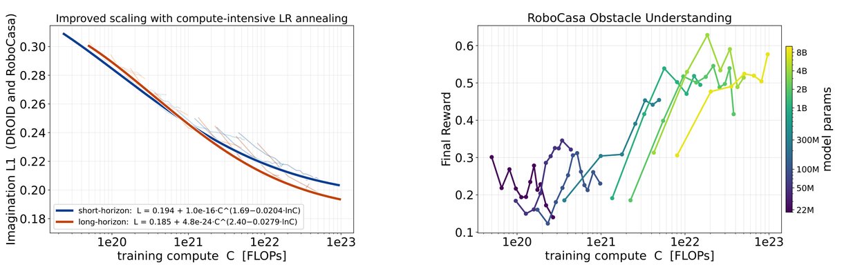
Figure 12: Imagination error scaling for short- vs. long-horizon prediction training.
图 12:短地平与长地平预测训练的想象误差缩放。
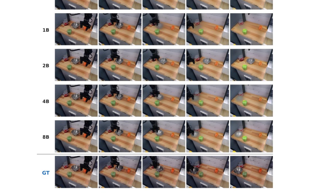
Figure 13: Obstacle-reach final reward, long-horizon prediction training.
图 13:长地平预测训练下的绕障到达最终奖励。
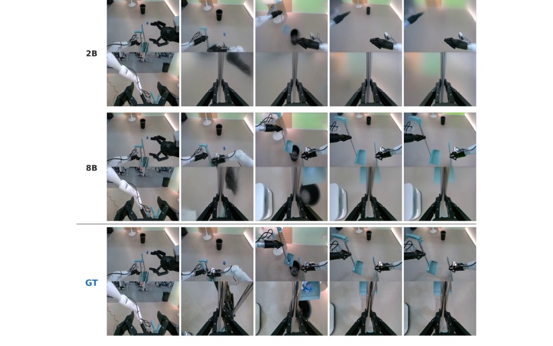
Figure 14: Longer-horizon prediction training improves scaling and downstream long-horizon planning. (a) Second-order scaling laws of the imagination error on DROID and RoboCasa for the two cooldown recipes. (b) Obstacle-reach final reward versus total training compute for the long-horizon (K = 10 ) models.
图 14:更长地平预测训练改善缩放与下游长地平规划。(a) 两种冷却配方在 DROID 与 RoboCasa 上的想象误差二阶缩放定律。(b) 长地平()模型的绕障到达最终奖励对总算力。
Figure 14 compares the two recipes by their scaling laws on DROID and RoboCasa. Long-horizon prediction training is more computationally expensive per step, but it becomes more compute-efficient beyond about 10 21 FLOPs of total training compute (around M– B parameters at the compute-optimal frontier) and reaches a substantially lower forward-prediction error. It also lowers the irreducible error of the fit, indicating a genuine reduction in error accumulation.
图 14 用 DROID 与 RoboCasa 上的缩放定律比较两种配方。长地平预测训练每步更贵,但在总算力约超过 FLOPs 后更算力高效(算力最优前沿大约对应 M–B 参数),并达到明显更低的前向预测误差;拟合的不可约误差也更低,表明误差累积被实质压低。
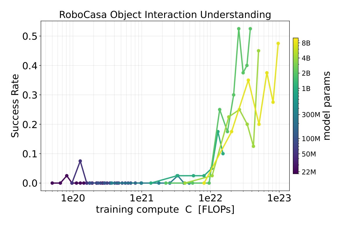
Figure 15: Downstream success rate on the RoboCasa push task versus training compute, for the long-horizon (K = 10 ) models.
图 15:长地平()模型在 RoboCasa 推物任务上的下游成功率对训练算力。
Deploying the non-greedy planning models on the obstacle-reach task (Figure 14) significantly improves the trend: the final reward now strongly follows the predictable scaling pattern. Small models (below M parameters) cap at around , which corresponds to the end-effector remaining stuck on the wrong side of the obstacle. The obstacle-avoidance capability then takes off around 10 21 FLOPs and saturates around 10 22 FLOPs. This is much later than the end-effector capabilities of Section 3.2, which emerged around 10 20 – 3 × 10 20 FLOPs, indicating that modeling interaction with the static scene geometry requires considerably more training.
把非贪心规划模型部署到绕障到达(图 14)后,趋势显著改善:最终奖励强力跟随可预期缩放模式。小模型(低于 M)封顶约在 ,对应末端卡在障碍物错误一侧。绕障能力约在 FLOPs 起跳,约在 FLOPs 饱和——远晚于第 3.2 节约 – FLOPs 出现的末端能力,说明建模与静态场景几何的交互需要多得多的训练。
Finally, the object-push task assesses the object interaction understanding (through non-greedy planning) by the world model: because the robot’s start and goal poses are identical (so the side and wrist views change only through the object’s position), the model must understand that pushing the object is what changes the scene. Figure 15 shows the success rate, defined simply as whether the object moved toward its target position (Section G.4). Interestingly, no model achieves a positive success rate until around 10 22 FLOPs, after which all models begin to succeed, suggesting that fine-grained understanding of surrounding objects emerges after certain training computation regardless of the model size. In summary, these results align in a natural order in which capabilities appear with more compute: first the 3D control of the end-effector, then manipulating a grasped object, then the geometry of the static scene, and finally the dynamics of objects in the scene.
最后,推物任务通过非贪心规划检验世界模型的物体交互理解:机器人起止位姿相同(侧视与腕视只因物体位置变化),模型必须理解「推动物体」才是改变场景的原因。图 15 给出成功率,定义为物体是否朝目标位置移动(附录 G.4)。有趣的是,直到约 FLOPs 之前没有任何模型取得正成功率,之后各规模都开始成功,暗示对周围物体的细粒度理解在达到一定训练算力后出现,而与模型规模关系较弱。综上,能力随算力出现的自然顺序是:末端三维控制 → 持物操作 → 静态场景几何 → 场景中物体动力学。
3.4 Real World Robotic Capabilities
3.4 真机机器人能力
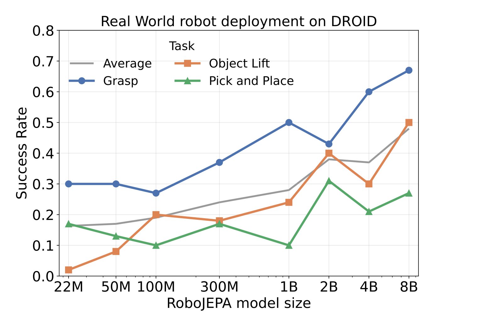
Figure 16: Real-world deployment on DROID. Success rates across model sizes for three manipulation tasks; the dashed line shows their average.
图 16:DROID 真机部署。三任务成功率随模型规模变化;虚线为平均。
Our ultimate goal is to showcase the capabilities of RoboJEPA in real-world settings. As a step towards this goal, we deploy RoboJEPA models ranging from 22M to 8B parameters on the DROID (Khazatsky et al., 2024) platform with a single-arm Franka robot and two cameras: an external camera mounted to the left of the arm and a wrist camera using the standard DROID mount. To deploy RoboJEPA via planning, we record an image goal on the robot by executing a predefined robot motion and manually placing the object in the grasping position so the robot can interact with it. We provide only a single final image goal, requiring longer-horizon, non-greedy planning. We evaluate three tasks: Grasp, Object Lift, and Pick and Place. We use the same planning hyperparameters across tasks and model sizes, evaluating the highest-compute checkpoint at each size. Setup, task definitions, episode counts, scoring criteria, and planning hyperparameters are detailed in Sections G.1 to G.3.
最终目标是展示 RoboJEPA 在真实世界中的能力。作为一步,我们在 DROID(Khazatsky 等,2024)平台上部署 22M 到 8B 的模型:单臂 Franka,外加左侧外置相机与标准 DROID 腕部相机。通过规划部署时,先执行预设运动并手动把物体放到可抓位置,从而在机器人上录制目标图像。只给一张最终目标图,因而需要更长地平的非贪心规划。评估三任务:Grasp、Object Lift、Pick and Place。跨任务与规模使用同一规划超参,并取各规模最高算力检查点。设置、任务定义、回合数、评分与超参见附录 G.1–G.3。
To contextualize the RoboJEPA results, we also evaluate the Vision-Language-Action (VLA) models π 0 -FAST (Pertsch et al., 2025) and π 0.5 (Black et al., 2025). However, their deployment differs in goal specification (text instructions versus a single goal image) and training (DROID fine-tuning for the VLA baselines versus pretraining on a mixture that includes DROID for RoboJEPA). Neither RoboJEPA nor the VLA baselines receive task-specific fine-tuning. These differences make the VLA results contextual references rather than directly comparable baselines. Figure 16 shows the scaling trend. For each task, all RoboJEPA models, including very small models, demonstrate non-zero success rates. Overall, success rates show a clear trend of improving with model size and generally decreasing with task complexity. This picture does not hold for the reference models, which work best on Pick and Place, the hardest task, but degrade significantly on the others. For example, π 0.5 achieves a 53 % success rate on Pick and Place but 0 % on Object Lift. We hypothesize that this difference may be an artifact of training, as verbs such as “lift” are heavily underrepresented in the DROID dataset, which focuses mostly on pick-and-place tasks. Due to the planning nature of the agent and the task specification as an image goal, RoboJEPA models are not susceptible to this type of degradation. Qualitatively, behavior transitioned gradually from smooth but less adaptive execution in smaller models to more reliable recovery from mistakes in larger models (Section G.7). Table 3 reports task progress and success rates for the largest RoboJEPA models and VLA references.
为给 RoboJEPA 结果提供语境,我们也评估视觉–语言–动作(VLA)模型 -FAST(Pertsch 等,2025)与 (Black 等,2025)。但二者在目标形式(文本指令 vs 单张目标图)与训练(VLA 基线做 DROID 微调 vs RoboJEPA 在含 DROID 的混合上预训练)上不同。双方都未做任务专属微调。这些差异使 VLA 结果只宜作语境参考,而非直接可比基线。图 16 显示缩放趋势:各任务上所有 RoboJEPA——包括很小的模型——都有非零成功率;总体随规模上升、随任务难度下降。参考模型则不然:它们在最难的 Pick and Place 最好,其他任务显著变差。例如 在 Pick and Place 上 53%,在 Object Lift 上 0%。我们猜测这可能是训练伪影:DROID 以抓取放置为主,「lift」等动词严重不足。RoboJEPA 以规划 + 图像目标指定任务,不易受此类退化。定性上,行为从较小模型较平滑但欠自适应,逐步过渡到较大模型更能从失误中恢复(附录 G.7)。表 3 报告最大 RoboJEPA 与 VLA 参考的任务进度与成功率。
Table 3: Real-robot task progress and success rates (%). Full results are in Table 12.
表 3:真机任务进度与成功率(%)。完整结果见表 12。
3.5 Qualitative Analysis
3.5 定性分析
So far we have quantified the world model through its prediction loss and downstream planning success; we now inspect how the prediction improves qualitatively by decoding its latent rollouts back to pixels. To do that, we use the diffusion decoder introduced in Section 2.3. The decoder serves purely as a visualization tool and is trained only on the frozen V-JEPA 2.1-G encoder features (see Appendix D). Note that all visualizations use the same encoder and decoder and vary only the RoboJEPA world model size. We perform forward prediction given a single frame (or a pair of frames) and a sequence of robot actions, and each sequence of predicted embeddings is decoded back to pixels. We run the prediction across a range of settings — low- and high-resolution, single- and dual-view — and report them separately (Figures 2 and 4; full set in Appendix E); the decoder itself is trained at a single 240 × 320 resolution. These visualizations show that the forward-prediction improves with model scale in several concrete ways: larger models track the true dynamics more accurately over the rollout, preserve object identity and fine manipulation detail, and keep multiple camera views mutually consistent. Several behaviors are effectively emergent with scale — gripper–object contact and structured deformation such as folding appear only once the predictor is large enough, whereas smaller models blur these interactions away. Finally, we finetune the B version of RoboJEPA on DROID to imagine all three camera views simultaneously at high ( p) resolution (Section C.4; Figure 17). These rollouts demonstrate that RoboJEPA performs accurate object manipulation even at very high resolution, and they exhibit strong cross-view information transfer, with content from the side (exterior) cameras propagating into the wrist-camera imagination.
至此我们用预测损失与下游规划成功量化了世界模型;现在把潜空间滚动解码回像素,定性观察预测如何随规模改善。使用第 2.3 节的扩散解码器:它仅作可视化,且只在冻结的 V-JEPA 2.1-G 编码器特征上训练(附录 D)。所有可视化共用同一编码器与解码器,只改 RoboJEPA 世界模型规模。给定单帧(或一对帧)与一段机器人动作做前向预测,再把预测嵌入序列解码为像素。我们在低/高分辨率、单/双视角等多种设定下分别报告(图 2、图 4;完整集见附录 E);解码器本身在单一 分辨率训练。可视化显示前向预测随规模在几方面具体改善:更大模型在滚动中更贴合真实动力学、更好保留物体身份与细操作细节,并保持多相机视角相互一致。若干行为近乎随规模涌现——夹爪–物体接触、折叠等结构化形变,只有预测器足够大才出现,较小模型会把这些交互糊掉。最后,我们在 DROID 上微调 B 版 RoboJEPA,使其在高分辨率(p)同时想象三路相机(附录 C.4;图 17)。这些滚动表明 RoboJEPA 在很高分辨率下仍能做准确物体操作,并展现强跨视角信息迁移:侧视(外置)内容会渗入腕部相机的想象。
4 Related Work
4 相关工作
Joint-Embedding Predictive Architectures. Joint-Embedding Predictive Architectures (JEPAs) were proposed as a path towards self-supervised models that learn abstract representations of the world by predicting in a latent space rather than at the pixel level (LeCun, 2022). I-JEPA (Assran et al., 2023) instantiated this recipe for images by predicting the representations of masked image regions from visible context, avoiding pixel-level reconstruction and the resulting collapse to low-level texture. V-JEPA extended the framework to video by predicting masked spatio-temporal feature regions and showed that the resulting features capture motion and temporal structure (Bardes et al., 2024). Assran et al. (2025) scaled feature prediction to over a million hours of internet video and, crucially for our setting, post-trained an action-conditioned predictor (V-JEPA 2-AC) on a small amount of unlabeled robot interaction data, enabling zero-shot Franka manipulation by latent planning against image goals. Our work, RoboJEPA, is similar to V-JEPA 2-AC in terms of the approach. We keep the V-JEPA encoder frozen and focus on the action-conditioned predictor as a world model. However, compared to V-JEPA 2 AC, we replace the small post-training corpus with a unified, large-scale mixture of robot demonstrations, therefore, the methods are not apples-to-apples comparable. To our knowledge, we provide the first systematic recipe for scaling V-JEPA-style action-conditioned predictors on large-scale, multi-embodiment robot data, and we characterize how predictor performance scales with parameters and demonstration tokens.
联合嵌入预测架构。联合嵌入预测架构(JEPA)被提出作为通向自监督模型的一条路径:在潜空间而非像素级预测,以学习世界的抽象表示(LeCun,2022)。I-JEPA(Assran 等,2023)把该配方实例化到图像:由可见上下文预测被掩图像区域的表示,避免像素重建及其向低层纹理坍缩。V-JEPA 将其扩展到视频,预测被掩时空特征区域,并表明所得特征捕捉运动与时间结构(Bardes 等,2024)。Assran 等(2025)把特征预测扩展到逾百万小时互联网视频,并——对我们的设定至关重要——在少量未标注机器人交互数据上后训练动作条件预测器(V-JEPA 2-AC),从而能以图像目标做潜空间规划、实现零样本 Franka 操作。本文 RoboJEPA 在方法上接近 V-JEPA 2-AC:冻结 V-JEPA 编码器,把动作条件预测器当作世界模型。但相对 V-JEPA 2-AC,我们用统一的大规模机器人演示混合取代小规模后训练语料,因而不能简单横向比较。据我们所知,我们首次给出在大规模、多本体机器人数据上缩放 V-JEPA 风格动作条件预测器的系统配方,并刻画预测器表现如何随参数与演示词元缩放。
World Models for Robotics. World models compress experience into a learned simulator of the environment that an agent can train and plan in (Ha and Schmidhuber, 2018). The Dreamer family pioneered this paradigm at scale: PlaNet learned latent dynamics for planning from pixels (Hafner et al., 2019), Dreamer used latent imagination to learn behaviors (Hafner et al., 2020), DreamerV2 introduced discrete latents to master Atari (Hafner et al., 2021), and DreamerV3 demonstrated a single set of hyperparameters that succeeds across a wide range of domains including 3D control (Hafner et al., 2023). DayDreamer applied Dreamer directly to physical robots and learned locomotion and manipulation in the real world (Wu et al., 2023), while Masked World Models showed that decoupling visual representation learning from dynamics modeling improves sample efficiency (Seo et al., 2023). More recent work has scaled video-based world models with transformer and diffusion backbones: IRIS (Micheli et al., 2023) and iVideoGPT (Wu et al., 2024a) treat world modeling as autoregressive token prediction; UniSim (Yang et al., 2024), Genie (Bruce et al., 2024), and GAIA-1 (Hu et al., 2023) train large generative simulators of interactive scenes; and the Cosmos platform releases physical-AI world foundation models at industrial scale (NVIDIA, 2025). In contrast to these pixel-space generators, RoboJEPA predicts in the representation space of a frozen V-JEPA encoder, which is what allows us to scale the predictor to billions of parameters on robot data without paying the computational cost of pixel-level reconstruction at every step.
机器人世界模型。世界模型把经验压缩成可训练、可规划的环境仿真器(Ha 与 Schmidhuber,2018)。Dreamer 系列把该范式做大:PlaNet 从像素学习潜动力学用于规划(Hafner 等,2019);Dreamer 用潜空间想象学行为(Hafner 等,2020);DreamerV2 引入离散潜变量以精通 Atari(Hafner 等,2021);DreamerV3 展示同一套超参可跨越含三维控制的广泛领域(Hafner 等,2023)。DayDreamer 把 Dreamer 直接用于物理机器人,在真机上学习运动与操作(Wu 等,2023);Masked World Models 则表明把视觉表示学习与动力学建模解耦可提高样本效率(Seo 等,2023)。更近的工作用 Transformer 与扩散骨干缩放基于视频的世界模型:IRIS(Micheli 等,2023)与 iVideoGPT(Wu 等,2024a)把世界建模当作自回归词元预测;UniSim(Yang 等,2024)、Genie(Bruce 等,2024)与 GAIA-1(Hu 等,2023)训练大型交互场景生成仿真器;Cosmos 平台则发布工业级物理 AI 世界基础模型(NVIDIA,2025)。与这些像素空间生成器不同,RoboJEPA 在冻结 V-JEPA 编码器的表示空间中预测,从而能在机器人数据上把预测器扩到数十亿参数,而不必每步支付像素级重建的计算代价。
Planning with Learned World Models. A central use of a world model is test-time planning. Classical model-based control methods such as PETS (Chua et al., 2018), model-based RL with neural network dynamics (Nagabandi et al., 2018), and visual foresight (Finn and Levine, 2017) optimize action sequences against a learned dynamics model. Sampling-based shooting methods, in particular the Cross-Entropy Method (Rubinstein, 1997; de Boer et al., 2005) and Model Predictive Path Integral control (Williams et al., 2017), remain the workhorses for high-dimensional action search. TD-MPC and TD-MPC2 combine latent dynamics, value learning, and CEM-style trajectory optimization for robust continuous control (Hansen et al., 2022; Hansen et al., 2024). DINO-WM (Zhou et al., 2025) learns task-agnostic dynamics in DINOv2 feature space from offline trajectories using an approximately M-parameter predictor, and uses CEM to plan toward image goals without additional task-specific training. RoboJEPA follows this line: at deployment, we use CEM in the latent space of the world model to score action sequences by how close their predicted features land to a goal image’s features, and execute the first action of the best plan in receding-horizon fashion.
用学到的世界模型做规划。世界模型的核心用途之一是测试时规划。经典基于模型的控制——如 PETS(Chua 等,2018)、带神经网络动力学的基于模型 RL(Nagabandi 等,2018)与视觉前瞻(Finn 与 Levine,2017)——相对学到的动力学优化动作序列。基于采样的射击法,尤其是交叉熵方法(Rubinstein,1997;de Boer 等,2005)与模型预测路径积分控制(Williams 等,2017),仍是高维动作搜索的主力。TD-MPC 与 TD-MPC2 结合潜动力学、价值学习与 CEM 风格轨迹优化,实现稳健连续控制(Hansen 等,2022;Hansen 等,2024)。DINO-WM(Zhou 等,2025)在 DINOv2 特征空间、从离线轨迹学习任务无关动力学(约 M 参数预测器),并用 CEM 朝图像目标规划、无需额外任务训练。RoboJEPA 沿此路线:部署时在世界模型潜空间用 CEM,按预测特征与目标图像特征的接近程度给动作序列打分,并以滚动地平方式执行最优计划的首个动作。
Closely related to our work, Terver et al. (2026) investigate how architectural, training, and planning choices affect latent world-model performance, including model and data scaling, albeit at smaller scales. Their proposed DROID predictor has approximately M parameters and is trained on an 8,000 -trajectory dataset. We extend this investigation both by scaling to substantially larger world models (up to B parameters) and datasets (a mixture of approximately M trajectories across robot platforms) and by explicitly studying their scaling behavior through scaling laws.
与我们密切相关的是 Terver 等(2026):他们研究架构、训练与规划选择如何影响潜空间世界模型表现,也包括模型与数据缩放,但尺度更小。其 DROID 预测器约 M 参数,训练于约 条轨迹。我们把调查扩展到显著更大的世界模型(至 B)与数据(约 M 条轨迹、跨 个机器人平台的混合),并显式通过缩放定律研究缩放行为。
Robotic Foundation Models from Demonstrations. A complementary line of work scales policies directly on robot demonstrations rather than scaling world models. RT-1 (Brohan et al., 2023) and RT-2 (Zitkovich et al., 2023) train large transformer- and vision-language-action policies on broad manipulation data. Open X-Embodiment Collaboration et al. (2023) aggregate demonstrations across many embodiments to enable cross-embodiment generalist policies, and a wave of recent generalist models such as Octo (Ghosh et al., 2024), OpenVLA (Kim et al., 2024), and π 0 (Black et al., 2024) push this behavior-cloning recipe further. RoboJEPA shares the same data substrate (in particular Open X-Embodiment, DROID (Khazatsky et al., 2024), RoboMIND (Wu et al., 2024b), BridgeData V2 (Walke et al., 2023), LeRobot (Cadene et al., 2024), and AgiBot World (AgiBot-World-Contributors et al., 2025)), but trains a goal-agnostic, action-conditioned predictive model instead of a task-conditioned policy. The same world model can then be used to evaluate or improve any policy, and to plan zero-shot for new goals at test time.
来自演示的机器人基础模型。互补路线是直接在机器人演示上缩放策略,而非缩放世界模型。RT-1(Brohan 等,2023)与 RT-2(Zitkovich 等,2023)在广泛操作数据上训练大型 Transformer 与视觉–语言–动作策略。Open X-Embodiment Collaboration 等(2023)汇聚多本体演示以支持跨本体通用策略;Octo(Ghosh 等,2024)、OpenVLA(Kim 等,2024)与 (Black 等,2024)等近期通用模型进一步推进行为克隆配方。RoboJEPA 共享同一数据底座(尤其 Open X-Embodiment、DROID、RoboMIND、BridgeData V2、LeRobot、AgiBot World),但训练的是目标无关、动作条件的预测模型,而非任务条件策略。同一个世界模型随后可用于评估或改进任意策略,并在测试时为零样本新目标做规划。
Scaling Laws. Power-law scaling of model loss with parameters, data, and compute has been documented extensively for language models (Kaplan et al., 2020), generative modeling more broadly (Henighan et al., 2020), and vision transformers (Zhai et al., 2022), with compute-optimal allocations of model and data established by Chinchilla (Hoffmann et al., 2022). In robotics, however, scaling laws are largely an open question because high-quality interaction data is scarce. We provide, to our knowledge, the first systematic scaling study for action-conditioned world models trained on large-scale, multi-embodiment real robot demonstrations, characterizing how forward-prediction loss scales with predictor parameters and demonstration tokens, and showing that this scaling behavior transfers to downstream planning performance.
缩放定律。模型损失相对参数、数据与算力的幂律缩放已在语言模型(Kaplan 等,2020)、更广的生成建模(Henighan 等,2020)与视觉 Transformer(Zhai 等,2022)上大量记载;Chinchilla(Hoffmann 等,2022)确立了模型与数据的算力最优分配。但在机器人领域,因高质量交互数据稀缺,缩放定律大体仍是开放问题。据我们所知,我们首次对在大规模、多本体真实机器人演示上训练的动作条件世界模型做系统缩放研究,刻画前向预测损失如何随预测器参数与演示词元缩放,并表明该缩放行为迁移到下游规划表现。
Scaling world models. A growing body of work reports that world models improve with scale. In autonomous driving, the GAIA line of latent-diffusion world models has been scaled to billions of parameters for controllable simulation and offline evaluation (Russell et al., 2025; Wayve, 2025; Wayve, 2026), though technical details beyond GAIA-2 are not publicly available. Pearce et al. (2024) fit power laws for pre-trained agents and world models and, in their appendix, report scaling laws for a robotic world model, but their study is otherwise centered on game and simulated environments rather than large-scale real-world multi-embodiment robot data. Sato et al. (2023) study how world-model quality varies with model size; IRASim (Zhu et al., 2025) reports empirical scaling trends for a fine-grained video world model for manipulation; PointWorld (Huang et al., 2026) shows that a 3D point-flow world model improves with more data and parameters; and DINO-world (Baldassarre et al., 2025) scales video prediction in the feature space of a frozen DINOv2 encoder using predictors with up to B parameters. Closest in spirit, τ 0 -VLA (Cai et al., 2026) scales test-time computation of a hierarchical policy using a world model to score candidate subtasks, and Dyna-2 (Dyna Robotics, 2026) scales a world-action model over a million hours of human and robot video and measures action -prediction quality. RoboJEPA differs from these along two axes: we scale training compute of a pure world model and measure its future-embedding (imagination) accuracy, and we fit an explicit scaling law rather than an empirical trend. This is a very important distinction, as an empirical scaling trend only establishes that a metric improves as one adds parameters, data, or compute, but says nothing about how much it will improve, whether returns have begun to saturate, or whether the next unit of budget is better spent on model size or on data. A scaling law, by contrast, is predictive: it extrapolates performance well beyond the scale at which it was fit, turning these decisions into quantitative forecasts. Establishing such predictive laws for action-conditioned robotic world models—and connecting them to downstream planning—is, to our knowledge, what sets this work apart.
缩放世界模型。越来越多工作报告世界模型随规模改善。自动驾驶中,GAIA 系列潜扩散世界模型已扩到数十亿参数,用于可控仿真与离线评估(Russell 等,2025;Wayve,2025;Wayve,2026),但 GAIA-2 之外的技术细节未公开。Pearce 等(2024)为预训练智能体与世界模型拟合幂律,并在附录报告机器人世界模型的缩放定律,但主体仍围绕游戏与仿真环境,而非大规模真实多本体机器人数据。Sato 等(2023)研究世界模型质量如何随模型大小变化;IRASim(Zhu 等,2025)报告细粒度视频世界模型用于操作的经验缩放趋势;PointWorld(Huang 等,2026)表明三维点流世界模型随数据与参数改善;DINO-world(Baldassarre 等,2025)在冻结 DINOv2 特征空间缩放视频预测,预测器至 B。精神上最接近的是 -VLA(Cai 等,2026)用世界模型给候选子任务打分以缩放分层策略的测试时计算,以及 Dyna-2(Dyna Robotics,2026)在逾百万小时人机视频上缩放世界–动作模型并度量动作预测质量。RoboJEPA 在两轴上不同:我们缩放的是纯世界模型的训练算力并度量其未来嵌入(想象)精度;我们拟合的是显式缩放定律而非经验趋势。这一区分很重要:经验趋势只说明加参数/数据/算力时指标变好,却不回答会好多少、回报是否开始饱和、下一单位预算该投模型还是数据。缩放定律则具有预测性:可在拟合尺度之外外推表现,把这些决策变成定量预报。据我们所知,为动作条件机器人世界模型建立此类可预测定律、并将其与下游规划相连,正是本文的独特之处。
5 Conclusion
5 结论
We introduced RoboJEPA, a family of action-conditioned latent world models trained on a large-scale, multi-embodiment robotic data collection in the latent space of V-JEPA 2.1. RoboJEPA predicts the next embedding in a single forward pass, and we train it to predict the future conditioned on past embeddings and future actions. We presented a recipe for scaling the predictor that works from 22M to 8B parameters, the latter being the largest JEPA predictor model trained to date. We then established scaling laws that predict the world-modeling error as we scale training compute. These take the form of a second-order power law L (C) = E + A C α − γ ln C . We established these laws for both a real-world (DROID) and a simulated (RoboCasa) embodiment. Finally, we demonstrated that offline prediction scaling laws correlate with the online downstream performance of world models, evaluated via planning toward a single image goal, which makes the offline imagination error a reliable proxy for real-robot evaluation and spares much of its computational cost. We also found that distinct manipulation capabilities emerge at their own compute thresholds, in a natural order from end-effector control, to manipulating a grasped object, to reasoning about static scene geometry, and finally to the dynamics of objects in the scene. On a real robot, we showed that the policy induced by world-model planning improves in success rate and in qualitative behavior as the world model scales. We also built a diffusion decoder to visualize the predicted action-conditioned future in pixel space, and used it to show that qualitatively better robotic predictions emerge with scale. We release all model checkpoints together with our training and robot-deployment code.
我们提出 RoboJEPA:在 V-JEPA 2.1 潜空间、于大规模多本体机器人数据上训练的动作条件潜空间世界模型族。RoboJEPA 单次前向预测下一嵌入,并在过去嵌入与未来动作条件下训练以预测未来。我们给出从 22M 到 8B 的预测器缩放配方,后者是迄今最大的 JEPA 预测器。随后建立随训练算力预测世界建模误差的缩放定律,形式为二阶幂律 ,并在真机(DROID)与仿真(RoboCasa)本体上分别确立。我们还表明,离线预测缩放定律与朝向单张图像目标规划所评估的在线下游表现相关,从而使离线想象误差成为真机评测的可靠代理,并省去大量算力开销。我们还发现,不同操作能力在各自的算力阈值涌现,顺序自然:末端控制 → 持物操作 → 静态场景几何 → 场景中物体动力学。在真机上,世界模型规划诱导的策略随世界模型缩放,在成功率与定性行为上都改善。我们还构建扩散解码器,在像素空间可视化动作条件的预测未来,并用以展示随规模涌现的定性更优机器人预测。我们公开全部模型检查点以及训练与真机部署代码。
Our study also has limitations that mark natural next steps. We scaled the predictor while keeping the V-JEPA 2.1 encoder frozen, so our laws describe a dynamics model on top of a fixed representation rather than the encoder and predictor jointly. Because we train for multiple epochs over a fixed corpus, our fits already sit close to data saturation, so pushing the frontier further will likely require more and more diverse interaction data rather than parameters alone. RoboJEPA also makes no use of text, planning instead toward a single image goal, and it makes no use of a learned policy proposal during planning, sampling actions from a uniform distribution and prioritizing them with the world model.
本研究亦有局限,标出自然的下一步。我们在冻结 V-JEPA 2.1 编码器的同时缩放预测器,故定律描述的是固定表示之上的动力学模型,而非编码器与预测器联合缩放。由于在固定语料上多轮训练,拟合已接近数据饱和;要继续推进前沿,更可能需要更多样的交互数据,而非仅堆参数。RoboJEPA 也不使用文本,而是朝向单张图像目标规划;规划时也不使用学到的提议策略,而是从均匀分布采样动作再由世界模型排序。
References
参考文献
1X Technologies (2024) 1X Technologies. 1X world model dataset. https://huggingface.co/datasets/1x-technologies/world_model_raw_data, 2024.
AgiBot-World-Contributors et al. (2025) AgiBot-World-Contributors, Qingwen Bu, Jisong Cai, Li Chen, Xiuqi Cui, Yan Ding, Siyuan Feng, Shenyuan Gao, Xindong He, Xuan Hu, Xu Huang, et al. AgiBot World Colosseo: A large-scale manipulation platform for scalable and intelligent embodied systems. arXiv preprint arXiv:2503.06669, 2025.
Ai et al. (2025) Bo Ai, Liu Dai, et al. Towards embodiment scaling laws in robot locomotion. In Conference on Robot Learning (CoRL), 2025.
Ainslie et al. (2023) Joshua Ainslie, James Lee-Thorp, Michiel de Jong, Yury Zemlyanskiy, Federico Lebrón, and Sumit Sanghai. GQA: Training generalized multi-query transformer models from multi-head checkpoints. In Empirical Methods in Natural Language Processing (EMNLP), 2023.
Ansel et al. (2024) Jason Ansel, Edward Yang, Horace He, Natalia Gimelshein, Animesh Jain, Michael Voznesensky, Bin Bao, Peter Bell, David Berard, Evgeni Burovski, Geeta Chauhan, Anjali Chourdia, Will Constable, Alban Desmaison, Zachary DeVito, Elias Ellison, Will Feng, Jiong Gong, Michael Gschwind, Brian Hirsh, Sherlock Huang, Kshiteej Kalambarkar, Laurent Kirsch, Michael Lazos, Mario Lezcano, Yanbo Liang, Jason Liang, Yinghai Lu, C. K. Luk, Bert Maher, Yunjie Pan, Christian Puhrsch, Matthias Reso, Mark Saroufim, Marcos Yukio Siraichi, Helen Suk, Michael Suo, Phil Tillet, Eikan Wang, Xiaodong Wang, William Wen, Shunting Zhang, Xu Zhao, Keren Zhou, Richard Zou, Ajit Mathews, Gregory Chanan, Peng Wu, and Soumith Chintala. PyTorch 2: Faster machine learning through dynamic Python bytecode transformation and graph compilation. In Proceedings of the 29th ACM International Conference on Architectural Support for Programming Languages and Operating Systems (ASPLOS), 2024. 10.1145/3620665.3640366.
Assran et al. (2023) Mahmoud Assran, Quentin Duval, Ishan Misra, Piotr Bojanowski, Pascal Vincent, Michael Rabbat, Yann LeCun, and Nicolas Ballas. Self-supervised learning from images with a joint-embedding predictive architecture. In IEEE/CVF Conference on Computer Vision and Pattern Recognition (CVPR), 2023.
Assran et al. (2025) Mahmoud Assran, Adrien Bardes, David Fan, Quentin Garrido, Russell Howes, Mojtaba Komeili, Matthew Muckley, Ammar Rizvi, Claire Roberts, Koustuv Sinha, Artem Zholus, Sergio Arnaud, Abha Gejji, Ada Martin, Francois Robert Hogan, Daniel Dugas, Piotr Bojanowski, Vasil Khalidov, Patrick Labatut, Francisco Massa, Marc Szafraniec, Kapil Krishnakumar, Yong Li, Xiaodong Ma, Sarath Chandar, Franziska Meier, Yann LeCun, Michael Rabbat, and Nicolas Ballas. V-JEPA 2: Self-supervised video models enable understanding, prediction and planning. arXiv preprint arXiv:2506.09985, 2025.
Baldassarre et al. (2025) Federico Baldassarre, Marc Szafraniec, Basile Terver, Vasil Khalidov, Francisco Massa, Yann LeCun, Patrick Labatut, Maximilian Seitzer, and Piotr Bojanowski. Back to the features: DINO as a foundation for video world models. arXiv preprint arXiv:2507.19468, 2025. https://arxiv.org/abs/2507.19468.
Bardes et al. (2024) Adrien Bardes, Quentin Garrido, Jean Ponce, Xinlei Chen, Michael Rabbat, Yann LeCun, Mahmoud Assran, and Nicolas Ballas. Revisiting feature prediction for learning visual representations from video. In Transactions on Machine Learning Research (TMLR), 2024.
Bharadhwaj et al. (2024) Homanga Bharadhwaj, Jay Vakil, Mohit Sharma, Abhinav Gupta, Shubham Tulsiani, and Vikash Kumar. RoboAgent: Generalization and efficiency in robot manipulation via semantic augmentations and action chunking. In IEEE International Conference on Robotics and Automation (ICRA), 2024.
Black et al. (2024) Kevin Black, Noah Brown, Danny Driess, Adnan Esmail, Michael Equi, Chelsea Finn, Niccolo Fusai, Lachy Groom, Karol Hausman, Brian Ichter, Szymon Jakubczak, Tim Jones, Liyiming Ke, Sergey Levine, Adrian Li-Bell, Mohith Mothukuri, Suraj Nair, Karl Pertsch, Lucy Xiaoyang Shi, James Tanner, Quan Vuong, Anna Walling, Haohuan Wang, and Ury Zhilinsky. π 0 : A vision-language-action flow model for general robot control. arXiv preprint arXiv:2410.24164, 2024.
Black et al. (2025) Kevin Black, Noah Brown, James Darpinian, Karan Dhabalia, Danny Driess, Adnan Esmail, Michael Equi, Chelsea Finn, Niccolo Fusai, Manuel Y. Galliker, Dibya Ghosh, Lachy Groom, Karol Hausman, Brian Ichter, Szymon Jakubczak, Tim Jones, Liyiming Ke, Devin LeBlanc, Sergey Levine, Adrian Li-Bell, Mohith Mothukuri, Suraj Nair, Karl Pertsch, Allen Z. Ren, Lucy Xiaoyang Shi, Laura Smith, Jost Tobias Springenberg, Kyle Stachowicz, James Tanner, Quan Vuong, Homer Walke, Anna Walling, Haohuan Wang, Lili Yu, and Ury Zhilinsky. π 0.5 : a vision-language-action model with open-world generalization. arXiv preprint arXiv:2504.16054, 2025.
Bordes et al. (2025) Florian Bordes, Quentin Garrido, Justine T Kao, Adina Williams, Michael Rabbat, and Emmanuel Dupoux. IntPhys 2: Benchmarking intuitive physics understanding in complex synthetic environments. arXiv preprint arXiv:2506.09849, 2025.
Brohan et al. (2023) Anthony Brohan, Noah Brown, Justice Carbajal, Yevgen Chebotar, Joseph Dabis, Chelsea Finn, Keerthana Gopalakrishnan, Karol Hausman, Alex Herzog, Jasmine Hsu, et al. RT-1: Robotics transformer for real-world control at scale. In Robotics: Science and Systems (RSS), 2023.
Bruce et al. (2024) Jake Bruce, Michael Dennis, Ashley Edwards, Jack Parker-Holder, Yuge Shi, Edward Hughes, Matthew Lai, Aditi Mavalankar, Richie Steigerwald, Chris Apps, Yusuf Aytar, Sarah Bechtle, Feryal Behbahani, Stephanie Chan, Nicolas Heess, Lucy Gonzalez, Simon Osindero, Sherjil Ozair, Scott Reed, Jingwei Zhang, Konrad Zolna, Jeff Clune, Nando de Freitas, Satinder Singh, and Tim Rocktäschel. Genie: Generative interactive environments. In International Conference on Machine Learning (ICML), 2024.
Caballero et al. (2022) Ethan Caballero, Kshitij Gupta, Irina Rish, and David Krueger. Broken neural scaling laws. arXiv preprint arXiv:2210.14891, 2022.
Caballero et al. (2026) Ethan Caballero, Priyank Jaini, David Krueger, and Irina Rish. Unified neural scaling laws. arXiv preprint arXiv:2605.26248, 2026.
Cadene et al. (2024) Remi Cadene, Simon Alibert, Alexander Soare, Quentin Gallouedec, Adil Zouitine, Steven Palma, Pepijn Kooijmans, Michel Aractingi, Mustafa Shukor, Dana Aubakirova, Martino Russi, Francesco Capuano, Caroline Pascal, Jade Choghari, Khalil Meftah, Maxime Ellerbach, Jess Moss, and Thomas Wolf. LeRobot: State-of-the-art machine learning for real-world robotics in PyTorch. https://github.com/huggingface/lerobot, 2024.
Cai et al. (2026) Xiaowei Cai, Yunuo Cai, Bingao Chen, Jingxiao Chen, Zhi Chen, Siyuan Feng, et al. τ 0 -VLA: a hierarchical robot foundation model with world-model-guided test-time computation. arXiv preprint arXiv:2608.16885, 2026.
Chen et al. (2024a) Boyuan Chen, Diego Martí Monsó, Yilun Du, Max Simchowitz, Russ Tedrake, and Vincent Sitzmann. Diffusion forcing: Next-token prediction meets full-sequence diffusion. In Advances in Neural Information Processing Systems (NeurIPS), volume 37, pages 24081–24125, 2024a. 10.52202/079017-0759. https://proceedings.neurips.cc/paper_files/paper/2024/hash/2aee1c4159e48407d68fe16ae8e6e49e-Abstract-Conference.html.
Chen et al. (2024b) Junsong Chen, Jincheng Yu, Chongjian Ge, Lewei Yao, Enze Xie, Yue Wu, Zhongdao Wang, James Kwok, Ping Luo, Huchuan Lu, and Zhenguo Li. PixArt- α : Fast training of diffusion transformer for photorealistic text-to-image synthesis. In International Conference on Learning Representations (ICLR), 2024b.
Chua et al. (2018) Kurtland Chua, Roberto Calandra, Rowan McAllister, and Sergey Levine. Deep reinforcement learning in a handful of trials using probabilistic dynamics models. In Advances in Neural Information Processing Systems (NeurIPS), 2018.
Dao (2024) Tri Dao. FlashAttention-2: Faster attention with better parallelism and work partitioning. In International Conference on Learning Representations (ICLR), 2024.
Dao et al. (2022) Tri Dao, Daniel Y. Fu, Stefano Ermon, Atri Rudra, and Christopher Ré. FlashAttention: Fast and memory-efficient exact attention with IO-awareness. In Advances in Neural Information Processing Systems (NeurIPS), 2022.
Dasari et al. (2019) Sudeep Dasari, Frederik Ebert, Stephen Tian, Suraj Nair, Bernadette Bucher, Karl Schmeckpeper, Siddharth Singh, Sergey Levine, and Chelsea Finn. RoboNet: Large-scale multi-robot learning. In Conference on Robot Learning (CoRL), 2019.
de Boer et al. (2005) Pieter-Tjerk de Boer, Dirk P. Kroese, Shie Mannor, and Reuven Y. Rubinstein. A tutorial on the cross-entropy method. Annals of Operations Research, 134(1):19–67, 2005.
Dehghani et al. (2023) Mostafa Dehghani, Josip Djolonga, Basil Mustafa, Piotr Padlewski, Jonathan Heek, Justin Gilmer, Andreas Steiner, Mathilde Caron, Robert Geirhos, Ibrahim Alabdulmohsin, Rodolphe Jenatton, Lucas Beyer, Michael Tschannen, Anurag Arnab, Xiao Wang, Carlos Riquelme, Matthias Minderer, Joan Puigcerver, Utku Evci, Manoj Kumar, Sjoerd van Steenkiste, Gamaleldin F. Elsayed, Aravindh Mahendran, Fisher Yu, Avital Oliver, Fantine Huot, Jasmijn Bastings, Mark Patrick Collier, Alexey Gritsenko, Vighnesh Birodkar, Cristina Vasconcelos, Yi Tay, Thomas Mensink, Alexander Kolesnikov, Filip Pavetić, Dustin Tran, Thomas Kipf, Mario Lučić, Xiaohua Zhai, Daniel Keysers, Jeremiah Harmsen, and Neil Houlsby. Scaling vision transformers to 22 billion parameters. In International Conference on Machine Learning (ICML), 2023.
Deng et al. (2009) Jia Deng, Wei Dong, Richard Socher, Li-Jia Li, Kai Li, and Li Fei-Fei. ImageNet: A large-scale hierarchical image database. In IEEE Conference on Computer Vision and Pattern Recognition (CVPR), 2009.
Dosovitskiy et al. (2021) Alexey Dosovitskiy, Lucas Beyer, Alexander Kolesnikov, Dirk Weissenborn, Xiaohua Zhai, Thomas Unterthiner, Mostafa Dehghani, Matthias Minderer, Georg Heigold, Sylvain Gelly, Jakob Uszkoreit, and Neil Houlsby. An image is worth 16x16 words: Transformers for image recognition at scale. In International Conference on Learning Representations (ICLR), 2021.
Dyna Robotics (2026) Dyna Robotics. Dyna-2: A 1-million-hour scaling law for world-action models. https://www.dyna.co/dyna-2, 2026. Accessed: 2026-09-04.
Ebert et al. (2022) Frederik Ebert, Yanlai Yang, Karl Schmeckpeper, Bernadette Bucher, Georgios Georgakis, Kostas Daniilidis, Chelsea Finn, and Sergey Levine. Bridge data: Boosting generalization of robotic skills with cross-domain datasets. In Robotics: Science and Systems (RSS), 2022.
Finn and Levine (2017) Chelsea Finn and Sergey Levine. Deep visual foresight for planning robot motion. In IEEE International Conference on Robotics and Automation (ICRA), 2017.
Ghosh et al. (2024) Dibya Ghosh, Homer Rich Walke, Karl Pertsch, Kevin Black, Oier Mees, Sudeep Dasari, Joey Hejna, Tobias Kreiman, Charles Xu, Jianlan Luo, You Liang Tan, Lawrence Yunliang Chen, Quan Vuong, Ted Xiao, Pannag R Sanketi, Dorsa Sadigh, Chelsea Finn, and Sergey Levine. Octo: An open-source generalist robot policy. In Proceedings of Robotics: Science and Systems, 2024. 10.15607/RSS.2024.XX.090. https://www.roboticsproceedings.org/rss20/p090.html.
Google DeepMind (2024) Google DeepMind. Genie 2: A large-scale foundation world model. https://deepmind.google/blog/genie-2-a-large-scale-foundation-world-model/, 2024. Technical report / blog post.
Ha and Schmidhuber (2018) David Ha and Jürgen Schmidhuber. Recurrent world models facilitate policy evolution. In Advances in Neural Information Processing Systems (NeurIPS), 2018.
Hafner et al. (2019) Danijar Hafner, Timothy Lillicrap, Ian Fischer, Ruben Villegas, David Ha, Honglak Lee, and James Davidson. Learning latent dynamics for planning from pixels. In International Conference on Machine Learning (ICML), 2019.
Hafner et al. (2020) Danijar Hafner, Timothy Lillicrap, Jimmy Ba, and Mohammad Norouzi. Dream to control: Learning behaviors by latent imagination. In International Conference on Learning Representations (ICLR), 2020.
Hafner et al. (2021) Danijar Hafner, Timothy Lillicrap, Mohammad Norouzi, and Jimmy Ba. Mastering Atari with discrete world models. In International Conference on Learning Representations (ICLR), 2021.
Hafner et al. (2023) Danijar Hafner, Jurgis Pasukonis, Jimmy Ba, and Timothy Lillicrap. Mastering diverse domains through world models. arXiv preprint arXiv:2301.04104, 2023.
Hafner et al. (2025) Danijar Hafner, Wilson Yan, and Timothy Lillicrap. Training agents inside of scalable world models. arXiv preprint arXiv:2509.24527, 2025.
Hansen et al. (2022) Nicklas Hansen, Xiaolong Wang, and Hao Su. Temporal difference learning for model predictive control. In International Conference on Machine Learning (ICML), 2022.
Hansen et al. (2024) Nicklas Hansen, Hao Su, and Xiaolong Wang. TD-MPC2: Scalable, robust world models for continuous control. In International Conference on Learning Representations (ICLR), 2024.
Hendrycks and Gimpel (2016) Dan Hendrycks and Kevin Gimpel. Gaussian error linear units (gelus). arXiv preprint arXiv:1606.08415, 2016.
Henighan et al. (2020) Tom Henighan, Jared Kaplan, Mor Katz, Mark Chen, Christopher Hesse, Jacob Jackson, Heewoo Jun, Tom B. Brown, Prafulla Dhariwal, Scott Gray, Chris Hallacy, Benjamin Mann, Alec Radford, Aditya Ramesh, Nick Ryder, Daniel M. Ziegler, John Schulman, Dario Amodei, and Sam McCandlish. Scaling laws for autoregressive generative modeling. arXiv preprint arXiv:2010.14701, 2020.
Ho and Salimans (2022) Jonathan Ho and Tim Salimans. Classifier-free diffusion guidance. arXiv preprint arXiv:2207.12598, 2022. https://arxiv.org/abs/2207.12598.
Ho et al. (2020) Jonathan Ho, Ajay Jain, and Pieter Abbeel. Denoising diffusion probabilistic models. In Advances in Neural Information Processing Systems (NeurIPS), 2020.
Hoffmann et al. (2022) Jordan Hoffmann, Sebastian Borgeaud, Arthur Mensch, Elena Buchatskaya, Trevor Cai, Eliza Rutherford, Diego de Las Casas, Lisa Anne Hendricks, Johannes Welbl, Aidan Clark, Thomas Hennigan, Eric Noland, Katherine Millican, George van den Driessche, Bogdan Damoc, Aurelia Guy, Simon Osindero, Karén Simonyan, Erich Elsen, Oriol Vinyals, Jack Rae, and Laurent Sifre. An empirical analysis of compute-optimal large language model training. In Advances in Neural Information Processing Systems (NeurIPS), volume 35, pages 30016–30030, 2022. 10.52202/068431-2176. https://proceedings.neurips.cc/paper_files/paper/2022/hash/c1e2faff6f588870935f114ebe04a3e5-Abstract.html.
Hoogeboom et al. (2023) Emiel Hoogeboom, Jonathan Heek, and Tim Salimans. simple diffusion: End-to-end diffusion for high resolution images. In International Conference on Machine Learning (ICML), 2023.
Hu et al. (2023) Anthony Hu, Lloyd Russell, Hudson Yeo, Zak Murez, George Fedoseev, Alex Kendall, Jamie Shotton, and Gianluca Corrado. GAIA-1: A generative world model for autonomous driving. arXiv preprint arXiv:2309.17080, 2023.
Hu et al. (2024) Shengding Hu, Yuge Tu, Xu Han, Chaoqun He, Ganqu Cui, Xiang Long, Zhi Zheng, Yewei Fang, Yuxiang Huang, Weilin Zhao, Xinrong Zhang, Zheng Leng Thai, Kaihuo Zhang, Chongyi Wang, Yuan Yao, Chenyang Zhao, Jie Zhou, Jie Cai, Zhongwu Zhai, Ning Ding, Chao Jia, Guoyang Zeng, Dahai Li, Zhiyuan Liu, and Maosong Sun. Minicpm: Unveiling the potential of small language models with scalable training strategies. arXiv preprint arXiv:2404.06395, 2024.
Huang et al. (2026) Wenlong Huang, Yu-Wei Chao, Arsalan Mousavian, Ming-Yu Liu, Dieter Fox, Kaichun Mo, et al. PointWorld: Scaling 3d world models for in-the-wild robotic manipulation. arXiv preprint arXiv:2601.03782, 2026.
Jang et al. (2022) Eric Jang, Alex Irpan, Mohi Khansari, Daniel Kappler, Frederik Ebert, Corey Lynch, Sergey Levine, and Chelsea Finn. BC-Z: Zero-shot task generalization with robotic imitation learning. In Conference on Robot Learning (CoRL), 2022.
Kalashnikov et al. (2018) Dmitry Kalashnikov, Alex Irpan, Peter Pastor, Julian Ibarz, Alexander Herzog, Eric Jang, Deirdre Quillen, Ethan Holly, Mrinal Kalakrishnan, Vincent Vanhoucke, and Sergey Levine. Scalable deep reinforcement learning for vision-based robotic manipulation. In Proceedings of The 2nd Conference on Robot Learning, volume 87 of Proceedings of Machine Learning Research, pages 651–673, 2018. https://proceedings.mlr.press/v87/kalashnikov18a.html.
Kalashnikov et al. (2021) Dmitry Kalashnikov, Jacob Varley, Yevgen Chebotar, Benjamin Swanson, Rico Jonschkowski, Chelsea Finn, Sergey Levine, and Karol Hausman. MT-Opt: Continuous multi-task robotic reinforcement learning at scale. arXiv preprint arXiv:2104.08212, 2021.
Kaplan et al. (2020) Jared Kaplan, Sam McCandlish, Tom Henighan, Tom B. Brown, Benjamin Chess, Rewon Child, Scott Gray, Alec Radford, Jeffrey Wu, and Dario Amodei. Scaling laws for neural language models. arXiv preprint arXiv:2001.08361, 2020.
Khazatsky et al. (2024) Alexander Khazatsky, Karl Pertsch, Suraj Nair, Ashwin Balakrishna, Sudeep Dasari, Siddharth Karamcheti, Soroush Nasiriany, Mohan Kumar Srirama, Lawrence Yunliang Chen, Kirsty Ellis, Peter David Fagan, Joey Hejna, Masha Itkina, Marion Lepert, Yecheng Jason Ma, Patrick Tree Miller, Jimmy Wu, Suneel Belkhale, Shivin Dass, Huy Ha, Arhan Jain, Abraham Lee, Youngwoon Lee, Marius Memmel, Sungjae Park, Ilija Radosavovic, Kaiyuan Wang, Albert Zhan, Kevin Black, Cheng Chi, Kyle Beltran Hatch, Shan Lin, Jingpei Lu, Jean Mercat, Abdul Rehman, Pannag R Sanketi, Archit Sharma, Cody Simpson, Quan Vuong, Homer Rich Walke, Blake Wulfe, Ted Xiao, Jonathan Heewon Yang, Arefeh Yavary, Tony Z. Zhao, Christopher Agia, Rohan Baijal, Mateo Guaman Castro, Daphne Chen, Qiuyu Chen, Trinity Chung, Jaimyn Drake, Ethan Paul Foster, Jensen Gao, Vitor Guizilini, David Antonio Herrera, Minho Heo, Kyle Hsu, Jiaheng Hu, Muhammad Zubair Irshad, Donovon Jackson, Charlotte Le, Yunshuang Li, Kevin Lin, Roy Lin, Zehan Ma, Abhiram Maddukuri, Suvir Mirchandani, Daniel Morton, Tony Nguyen, Abigail O’Neill, Rosario Scalise, Derick Seale, Victor Son, Stephen Tian, Emi Tran, Andrew E. Wang, Yilin Wu, Annie Xie, Jingyun Yang, Patrick Yin, Yunchu Zhang, Osbert Bastani, Glen Berseth, Jeannette Bohg, Ken Goldberg, Abhinav Gupta, Abhishek Gupta, Dinesh Jayaraman, Joseph J Lim, Jitendra Malik, Roberto Martín-Martín, Subramanian Ramamoorthy, Dorsa Sadigh, Shuran Song, Jiajun Wu, Michael C. Yip, Yuke Zhu, Thomas Kollar, Sergey Levine, and Chelsea Finn. DROID: A large-scale in-the-wild robot manipulation dataset. arXiv preprint arXiv:2403.12945, 2024.
Kim et al. (2024) Moo Jin Kim, Karl Pertsch, Siddharth Karamcheti, Ted Xiao, Ashwin Balakrishna, Suraj Nair, Rafael Rafailov, Ethan Foster, Grace Lam, Pannag Sanketi, Quan Vuong, Thomas Kollar, Benjamin Burchfiel, Russ Tedrake, Dorsa Sadigh, Sergey Levine, Percy Liang, and Chelsea Finn. OpenVLA: An open-source vision-language-action model. In Conference on Robot Learning (CoRL), 2024.
LeCun (2022) Yann LeCun. A path towards autonomous machine intelligence. Open Review, 2022. https://openreview.net/forum?id=BZ5a1r-kVsf.
Lin et al. (2025) Fanqi Lin, Yingdong Hu, Pingyue Sheng, Chuan Wen, Jiacheng You, and Yang Gao. Data scaling laws in imitation learning for robotic manipulation. In International Conference on Learning Representations (ICLR), 2025.
Lin et al. (2024) Shanchuan Lin, Bingchen Liu, Jiashi Li, and Xiao Yang. Common diffusion noise schedules and sample steps are flawed. In IEEE/CVF Winter Conference on Applications of Computer Vision (WACV), 2024.
Loshchilov and Hutter (2019) Ilya Loshchilov and Frank Hutter. Decoupled weight decay regularization. In International Conference on Learning Representations (ICLR), 2019.
Luo et al. (2024) Jianlan Luo, Charles Xu, Fangchen Liu, Liam Tan, Zipeng Lin, Jeffrey Wu, Pieter Abbeel, and Sergey Levine. FMB: A functional manipulation benchmark for generalizable robotic learning. The International Journal of Robotics Research, 2024.
Lynch et al. (2023) Corey Lynch, Ayzaan Wahid, Jonathan Tompson, Tianli Ding, James Betker, Robert Baruch, Travis Armstrong, and Pete Florence. Interactive language: Talking to robots in real time. In IEEE Robotics and Automation Letters (RA-L), 2023.
Mayne et al. (2000) D. Q. Mayne, J. B. Rawlings, C. V. Rao, and P. O. M. Scokaert. Constrained model predictive control: Stability and optimality. Automatica, 36(6):789–814, 2000. 10.1016/S0005-1098(99)00214-9.
Micheli et al. (2023) Vincent Micheli, Eloi Alonso, and François Fleuret. Transformers are sample-efficient world models. In International Conference on Learning Representations (ICLR), 2023.
Mur-Labadia et al. (2026) Lorenzo Mur-Labadia, Matthew Muckley, Amir Bar, Mido Assran, Koustuv Sinha, Mike Rabbat, Yann LeCun, Nicolas Ballas, and Adrien Bardes. V-JEPA 2.1: Unlocking dense features in video self-supervised learning. arXiv preprint arXiv:2603.14482, 2026.
Nagabandi et al. (2018) Anusha Nagabandi, Gregory Kahn, Ronald S. Fearing, and Sergey Levine. Neural network dynamics for model-based deep reinforcement learning with model-free fine-tuning. In IEEE International Conference on Robotics and Automation (ICRA), 2018.
Nasiriany et al. (2024) Soroush Nasiriany, Abhiram Maddukuri, Lance Zhang, Adeet Parikh, Aaron Lo, Abhishek Joshi, Ajay Mandlekar, and Yuke Zhu. RoboCasa: Large-scale simulation of everyday tasks for generalist robots. In Robotics: Science and Systems (RSS), 2024.
Nasiriany et al. (2026) Soroush Nasiriany, Sepehr Nasiriany, Abhiram Maddukuri, and Yuke Zhu. RoboCasa365: A large-scale simulation framework for training and benchmarking generalist robots. arXiv preprint arXiv:2603.04356, 2026.
Nichol and Dhariwal (2021) Alexander Quinn Nichol and Prafulla Dhariwal. Improved denoising diffusion probabilistic models. In International Conference on Machine Learning (ICML), 2021.
Nilaksh et al. (2026) Nilaksh, Saurav Jha, Artem Zholus, and Sarath Chandar. Reconstruction or semantics? what makes a latent space useful for robotic world models. arXiv preprint arXiv:2605.06388, 2026. https://arxiv.org/abs/2605.06388.
NVIDIA (2025) NVIDIA. Cosmos world foundation model platform for physical AI. arXiv preprint arXiv:2501.03575, 2025.
Open X-Embodiment Collaboration et al. (2023) Open X-Embodiment Collaboration, Abby O’Neill, Abdul Rehman, Abhinav Gupta, Abhiram Maddukuri, Abhishek Gupta, Abhishek Padalkar, Abraham Lee, Acorn Pooley, Agrim Gupta, Ajay Mandlekar, Ajinkya Jain, et al. Open X-embodiment: Robotic learning datasets and RT-X models. arXiv preprint arXiv:2310.08864, 2023.
PAN Team et al. (2025) PAN Team, Jiannan Xiang, Yi Gu, Zihan Liu, Zeyu Feng, Qiyue Gao, Yiyan Hu, Benhao Huang, Guangyi Liu, Yichi Yang, Kun Zhou, et al. PAN: A world model for general, interactable, and long-horizon world simulation. arXiv preprint arXiv:2511.09057, 2025. https://arxiv.org/abs/2511.09057v1.
Pearce and Song (2024) Tim Pearce and Jinyeop Song. Reconciling kaplan and chinchilla scaling laws. arXiv preprint arXiv:2406.12907, 2024.
Pearce et al. (2024) Tim Pearce, Tabish Rashid, Dave Bignell, Raluca Georgescu, Sam Devlin, and Katja Hofmann. Scaling laws for pre-training agents and world models. arXiv preprint arXiv:2411.04434, 2024.
Peebles and Xie (2023) William Peebles and Saining Xie. Scalable diffusion models with transformers. In IEEE/CVF International Conference on Computer Vision (ICCV), 2023.
Pertsch et al. (2025) Karl Pertsch, Kyle Stachowicz, Brian Ichter, Danny Driess, Suraj Nair, Quan Vuong, Oier Mees, Chelsea Finn, and Sergey Levine. FAST: Efficient action tokenization for vision-language-action models. arXiv preprint arXiv:2501.09747, 2025.
Po et al. (2025) Ryan Po, Yotam Nitzan, Richard Zhang, Berlin Chen, Tri Dao, Eli Shechtman, Gordon Wetzstein, and Xun Huang. Long-context state-space video world models. arXiv preprint arXiv:2505.20171, 2025.
Punzo et al. (2026) Samuele Punzo, Niccolò Caselli, Ippokratis Pantelidis, Francesco Massafra, Salvatore Lo Sardo, and Mohammadreza Salehi. How do video foundation models encode intuitive physics? probing across pretraining paradigms. arXiv preprint arXiv:2606.09646, 2026.
Rubinstein (1997) Reuven Y. Rubinstein. Optimization of computer simulation models with rare events. European Journal of Operational Research, 99(1):89–112, 1997.
Russell et al. (2025) Lloyd Russell, Anthony Hu, Lorenzo Bertoni, George Fedoseev, Jamie Shotton, Elahe Arani, and Gianluca Corrado. GAIA-2: A controllable multi-view generative world model for autonomous driving. arXiv preprint arXiv:2503.20523, 2025.
Sartor and Thompson (2024) Sebastian Sartor and Neil C. Thompson. Neural scaling laws in robotics. arXiv preprint arXiv:2405.14005, 2024.
Sato et al. (2023) Makoto Sato, Ryosuke Unno, Masahiro Negishi, Koudai Tabata, Taiju Watanabe, Junnosuke Kamohara, Taiga Kume, Ryo Okada, Yusuke Iwasawa, and Yutaka Matsuo. Scaling laws of model size for world models. In Proceedings of the Annual Conference of the Japanese Society for Artificial Intelligence (JSAI), 2023. 10.11517/pjsai.JSAI2023.0_2G5OS21e02. In Japanese.
Seo et al. (2023) Younggyo Seo, Danijar Hafner, Hao Liu, Fangchen Liu, Stephen James, Kimin Lee, and Pieter Abbeel. Masked world models for visual control. In Conference on Robot Learning (CoRL), 2023.
Song et al. (2021) Jiaming Song, Chenlin Meng, and Stefano Ermon. Denoising diffusion implicit models. In International Conference on Learning Representations (ICLR), 2021.
Su et al. (2024) Jianlin Su, Murtadha Ahmed, Yu Lu, Shengfeng Pan, Wen Bo, and Yunfeng Liu. RoFormer: Enhanced transformer with rotary position embedding. Neurocomputing, 568:127063, 2024.
Terver et al. (2026) Basile Terver, Tsung-Yen Yang, Jean Ponce, Adrien Bardes, and Yann LeCun. What drives success in physical planning with joint-embedding predictive world models? Transactions on Machine Learning Research, 2026. https://openreview.net/forum?id=cHZn5Gdh8e.
Walke et al. (2023) Homer Walke, Kevin Black, Abraham Lee, Moo Jin Kim, Max Du, Chongyi Zheng, Tony Zhao, Philippe Hansen-Estruch, Quan Vuong, Andre He, Vivek Myers, Kuan Fang, Chelsea Finn, and Sergey Levine. BridgeData V2: A dataset for robot learning at scale. In Conference on Robot Learning (CoRL), 2023.
Wayve (2025) Wayve. GAIA-3: Scaling world models to power safety and evaluation. https://wayve.ai/thinking/gaia-3/, 2025. Accessed: 2026-09-04.
Wayve (2026) Wayve. GAIA-4: Multimodal world models powering closed-loop simulation for safe and scalable autonomy. https://wayve.ai/thinking/gaia-4/, 2026. Accessed: 2026-09-04.
Williams et al. (2017) Grady Williams, Nolan Wagener, Brian Goldfain, Paul Drews, James M. Rehg, Byron Boots, and Evangelos A. Theodorou. Information theoretic MPC for model-based reinforcement learning. In IEEE International Conference on Robotics and Automation (ICRA), 2017. 10.1109/ICRA.2017.7989202.
Wu et al. (2024a) Jialong Wu, Shaofeng Yin, Ningya Feng, Xu He, Dong Li, Jianye Hao, and Mingsheng Long. iVideoGPT: Interactive VideoGPTs are scalable world models. In Advances in Neural Information Processing Systems (NeurIPS), 2024a.
Wu et al. (2024b) Kun Wu, Chengkai Hou, Jiaming Liu, Zhengping Che, Xiaozhu Ju, Zhuqin Yang, Meng Li, Yinuo Zhao, Zhiyuan Xu, Guang Yang, Zhen Zhao, Guangyu Li, Zhao Jin, Lecheng Wang, Jilei Mao, Xinhua Wang, Shichao Fan, Ning Liu, Pei Ren, Qiang Zhang, Yaoxu Lyu, Mengzhen Liu, Jingyang He, Yulin Luo, Zeyu Gao, Chenxuan Li, Chenyang Gu, Yankai Fu, Di Wu, Xingyu Wang, Sixiang Chen, Zhenyu Wang, Pengju An, Siyuan Qian, Shanghang Zhang, and Jian Tang. RoboMIND: Benchmark on multi-embodiment intelligence normative data for robot manipulation. arXiv preprint arXiv:2412.13877, 2024b. https://arxiv.org/abs/2412.13877v1.
Wu et al. (2023) Philipp Wu, Alejandro Escontrela, Danijar Hafner, Ken Goldberg, and Pieter Abbeel. DayDreamer: World models for physical robot learning. In Conference on Robot Learning (CoRL), 2023.
Yang et al. (2024) Sherry Yang, Yilun Du, Seyed Ghasemipour, Jonathan Tompson, Leslie Kaelbling, Dale Schuurmans, and Pieter Abbeel. Learning interactive real-world simulators. In International Conference on Learning Representations (ICLR), pages 45210–45234, 2024. https://proceedings.iclr.cc/paper_files/paper/2024/hash/c4d66eae503694424123b93ac0fbaf17-Abstract-Conference.html.
Zhai et al. (2022) Xiaohua Zhai, Alexander Kolesnikov, Neil Houlsby, and Lucas Beyer. Scaling vision transformers. In IEEE/CVF Conference on Computer Vision and Pattern Recognition (CVPR), 2022.
Zhang and Sennrich (2019) Biao Zhang and Rico Sennrich. Root mean square layer normalization. Advances in Neural Information Processing Systems (NeurIPS), 2019.
Zhang et al. (2026) Wancong Zhang, Basile Terver, Artem Zholus, Soham Chitnis, Harsh Sutaria, Mido Assran, Randall Balestriero, Amir Bar, Adrien Bardes, Yann LeCun, et al. Hierarchical planning with latent world models. arXiv preprint arXiv:2604.03208, 2026.
Zhou et al. (2025) Gaoyue Zhou, Hengkai Pan, Yann LeCun, and Lerrel Pinto. DINO-WM: World models on pre-trained visual features enable zero-shot planning. In Proceedings of the 42nd International Conference on Machine Learning, volume 267 of Proceedings of Machine Learning Research, pages 79115–79135. PMLR, 2025. https://proceedings.mlr.press/v267/zhou25t.html.
Zhu et al. (2025) Fangqi Zhu, Hongtao Wu, Song Guo, Yuxiao Liu, Chilam Cheang, and Tao Kong. IRASim: A fine-grained world model for robot manipulation. In Proceedings of the IEEE/CVF International Conference on Computer Vision (ICCV), 2025.
Zitkovich et al. (2023) Brianna Zitkovich, Tianhe Yu, Sichun Xu, Peng Xu, Ted Xiao, Fei Xia, Jialin Wu, Paul Wohlhart, Stefan Welker, Ayzaan Wahid, Quan Vuong, Vincent Vanhoucke, Huong Tran, Radu Soricut, Anikait Singh, Jaspiar Singh, Pierre Sermanet, Pannag R. Sanketi, Grecia Salazar, Michael S. Ryoo, Krista Reymann, Kanishka Rao, Karl Pertsch, Igor Mordatch, Henryk Michalewski, Yao Lu, Sergey Levine, Lisa Lee, Tsang-Wei Edward Lee, Isabel Leal, Yuheng Kuang, Dmitry Kalashnikov, Ryan Julian, Nikhil J. Joshi, Alex Irpan, Brian Ichter, Jasmine Hsu, Alexander Herzog, Karol Hausman, Keerthana Gopalakrishnan, Chuyuan Fu, Pete Florence, Chelsea Finn, Kumar Avinava Dubey, Danny Driess, Tianli Ding, Krzysztof Marcin Choromanski, Xi Chen, Yevgen Chebotar, Justice Carbajal, Noah Brown, Anthony Brohan, Montserrat Gonzalez Arenas, and Kehang Han. RT-2: Vision-language-action models transfer web knowledge to robotic control. In Jie Tan, Marc Toussaint, and Kourosh Darvish, editors, Proceedings of The 7th Conference on Robot Learning, volume 229 of Proceedings of Machine Learning Research, pages 2165–2183. PMLR, 06–09 Nov 2023. https://proceedings.mlr.press/v229/zitkovich23a.html.
Appendix A Model Architecture: Additional Details
附录 A 模型架构:补充细节
Expands Section 2.1. We collect here the implementation-level details of the predictor block: the channel-pair derivation behind factorised RoPE (Section A.1); the per-block view bias under grouped-query attention (Section A.2); the per-embodiment input projection (Section A.4); the embodiment-id breakdown that yields | ℰ | = 26 (Section A.5); and the predictor scaling sweep across all eight scales used in the scaling law of Section 3 (Section A.6). All notation is shared with Section 2.1; in particular, ℓ is reserved for the predictor layer index and τ for autoregressive rollout steps.
扩展第 2.1 节。此处汇总预测器块的实现级细节:因子化 RoPE 背后的通道对推导(A.1);分组查询注意力下的逐块视角偏置(A.2);按本体的输入投影(A.4);给出 的本体 id 分解(A.5);以及第 3 节缩放定律所用全部八个规模的预测器扫描(A.6)。记号与第 2.1 节一致:尤其 专指预测器层索引, 专指自回归滚动步。
Table 4 summarises how the RoboJEPA predictor differs from the action-conditioned V-JEPA 2 predictor (V-JEPA 2-AC) (Assran et al., 2025) it builds on. The two share the same backbone family and the same next-frame prediction parameterisation; RoboJEPA changes the normalisation, position encoding, and the conditioning that supports cross-view, cross-embodiment world modeling.
表 4 概括 RoboJEPA 预测器相对其所基于的动作条件 V-JEPA 2 预测器(V-JEPA 2-AC)(Assran 等,2025)有何不同。二者共享同一骨干族与同一下一帧预测参数化;RoboJEPA 改动了归一化、位置编码,以及支撑跨视角、跨本体世界建模的条件化。
Table 4: Architectural comparison between the action-conditioned V-JEPA 2 predictor (V-JEPA 2-AC) (Assran et al., 2025) and the RoboJEPA predictor. Both share the V-JEPA 2 backbone and the next-frame latent-prediction parameterisation; RoboJEPA adds RMSNorm and QK-norm for training stability at scale, a fourth (view) RoPE axis, and explicit per-embodiment and per-view conditioning for cross-embodiment, multi-view world modeling.
表 4:动作条件 V-JEPA 2 预测器(V-JEPA 2-AC)(Assran 等,2025)与 RoboJEPA 预测器的架构对比。二者共享 V-JEPA 2 骨干与下一帧潜预测参数化;RoboJEPA 增加 RMSNorm 与 QK-norm 以利大规模训练稳定,增加第四(视角)RoPE 轴,以及显式的按本体、按视角条件,以支持跨本体、多视角世界建模。
A.1 Factorised multi-axis RoPE
A.1 因子化多轴 RoPE
Each per-head channel space { 0, …, d h − 1 } partitions into four contiguous, equal-size sub-blocks of width d ax = d h / 4 , one per spatio-temporal axis. Fix the enumeration 𝒜 max = { t, i, j, v } for the time, height, width, and view axes, and let j α denote the starting channel of axis α , so
每个头的通道空间 被划分为四个连续、等宽子块,宽 ,各对应一个时空轴。固定枚举 表示时间、高、宽、视角轴,并以 记轴 的起始通道,于是
Under multi-view training (V max = 2 ) we use the full 4-axis partition 𝒜 = { t, i, j, v } : the -axis sub-block contributes its own rotation, and viewpoint identity is additionally supplied by the per-block additive bias of Section A.2 (the two are complementary). For purely single-view runs (V = 1 ) the -axis sub-block carries no rotation and is left as the identity. Action and state tokens are detached from the visual slab before the RoPE rotation is applied: only the time component of RoPE rotates them (indexed by their step id), so that a single proprioceptive token per step does not spuriously inherit a spatial position.
多视角训练()时使用完整四轴划分 : 轴子块贡献自有旋转,视角身份另由 A.2 节的逐块加性偏置提供(二者互补)。纯单视角()时 轴子块不旋转、保持恒等。动作与状态词元在施加 RoPE 前从视觉板分离:只对它们施加 RoPE 的时间分量(按步 id 索引),以免每步单个本体词元错误继承空间位置。
A.2 Per-block view bias under grouped-query attention
A.2 分组查询注意力下的逐块视角偏置
The view information is encoded into the model in two ways. First, the view position encoding disambiguates different views of tokens with the same spatio-temporal position. This is achieved by rotating the view-axis sub-block (d h / 4 channels per head). However, the view position only informs the model that two different views are distinct without any encoding of the type of the content (e.g. the model has to know which view represents the side camera looking from the left and which one is mounted on the wrist). One way of dealing with it is to just let the model learn this end-to-end; however, we decided to directly inject the view information as a learnable bias added across the full head width of visual-token queries and keys after the four-axis RoPE rotation:
视角信息以两种方式编入模型。其一,视角位置编码区分具有相同时空位置的不同视角词元,做法是旋转视角轴子块(每头 通道)。但视角位置只告诉模型两视角不同,并不编码内容类型(例如须知哪路是左侧侧视、哪路是腕部)。一端到端学习也可以,但我们选择在四轴 RoPE 之后,直接把视角信息作为可学习偏置加到视觉词元查询与键的整个头宽上:
The strong-view conditioning of Equation 9 is a zero-initialised, layer-wise additive bias indexed by the semantic camera id c (v) ∈ 𝒱 (left, right, wrist, front, back, head, top), implemented as U ℓ ∈ ℝ | 𝒱 | × d h for each ℓ ∈ { 1, …, N layers } and added to all d h channels of every visual token’s queries and keys after the RoPE rotation of Equation 8. Concretely, let Q ℓ ∈ ℝ N × h q × d h and K ℓ ∈ ℝ N × h k v × d h be the post-RoPE query and key tensors of layer ℓ for a per-step token bag of length , and let b ℓ (v):= U ℓ [ c (v) ] ∈ ℝ d h be the bias gathered for view . Under grouped-query attention (Ainslie et al., 2023) with h q query heads and h k v KV heads sharing the same head dimension d h , the bias is added by the broadcast rule
式 9 的强视角条件是零初始化、按层的加性偏置,由语义相机 id (left、right、wrist、front、back、head、top)索引,实现为每层 的,并在式 8 的 RoPE 旋转之后加到每个视觉词元查询与键的全部 通道。具体地,令 、 为层 、长度 的逐步词元袋在 RoPE 后的查询与键张量,并令 为视角 取到的偏置。在分组查询注意力(Ainslie 等,2023)下, 个查询头与 个共享头维 的 KV 头按广播规则相加偏置
This per-layer additive bias supplements the -axis RoPE rotation of Equation 6: under our default strong-view configuration both signals are active, the rotation contributes a relative-view phase to attention scores, and the bias contributes a d h -wide per-layer per-camera offset on top of it. The combination gives a stable handle on viewpoint identity for multi-view planning (Section 2.2); zero initialisation of U ℓ makes loading a checkpoint trained without strong view conditioning a no-op at step .
该逐层加性偏置补充式 6 的 轴 RoPE 旋转:在默认强视角配置下两信号同时生效,旋转为注意力分数贡献相对视角相位,偏置再叠加 宽的逐层、逐相机偏移。组合为多视角规划提供稳定的视角身份把手(第 2.2 节); 零初始化使得加载未用强视角条件训练的检查点在第 步是空操作。
A.3 Attention masking
A.3 注意力掩码
We use a similar attention mask to V-JEPA 2-AC (Assran et al., 2025) but extend it to multiple views: attention is timestep-level causal and restricted to a local temporal window of timesteps, while within a step all V H p W p visual tokens (plus the action and state tokens) attend omnidirectionally (any-to-any). More precisely, the rasterized sequence of tokens has T × N tok tokens in total and the token at index can attend to tokens with indices such that ⌊ k N tok ⌋ − 7 ⩽ ⌊ j N tok ⌋ ⩽ ⌊ k N tok ⌋ . Schematically, this means that packing the sequence as frame-blocks of size N tok given by Equation 20, the attention mask between blocks is banded lower-triangular: each block of size N tok × N tok is fully attended within the diagonal band of width W t and zero outside it. This trick makes the computational cost of attention grow linearly as a function of the step number and it alleviates the problem of the position extrapolation – the predicted content quality depends only on the accumulated error, not the ability of the model to extrapolate, because it never observes a sequence longer than the window size. This is a classical trick for language models and world models (Assran et al., 2025; Po et al., 2025; PAN Team et al., 2025). The bounded window keeps the per-step computational cost of attention constant and makes the predictor KV-cacheable in 𝒪 (W t ⋅ V ⋅ H p ⋅ W p) keys per layer; Section 2.2 uses this at deployment.
我们使用与 V-JEPA 2-AC(Assran 等,2025)类似的注意力掩码,但扩展到多视角:注意力在时间步级因果,并限制在 个时间步的局部时间窗内;同一步内全部 个视觉词元(外加动作与状态词元)全互连(any-to-any)。更精确地,光栅化词元序列共有 个词元,索引 的词元可关注满足 的索引 。示意上,按式 20 把序列打成大小为 的 个帧块后,块间注意力掩码是带宽下三角:每个 块在宽为 的对角带内全互连,带外为零。该技巧使注意力计算量随步数线性增长,并缓解位置外推问题——预测内容质量只依赖累积误差,而不依赖模型外推能力,因为它从未见到超过窗口的序列。这是语言模型与世界模型中的经典做法(Assran 等,2025;Po 等,2025;PAN Team 等,2025)。有界窗口使每步注意力代价恒定,并使预测器可按每层 键做 KV 缓存;第 2.2 节在部署时使用。
A.4 Per-embodiment input projection
A.4 按本体的输入投影
Every embodiment owns its own input weight matrix W a (e) in a single multi-embodiment linear projection. The raw action vector a t ∈ ℝ d a is zero-padded to a common width d a max jointly large enough to absorb the widest action convention in our mixture (Section 2.2; for the 1B run d a max = d s max = 64 , set by the chunked DROID joint_vel action-key variant which produces an ⋅ = 64 -D mega-action) before projection,
每个本体 在单一多本体线性投影中拥有自己的输入权重矩阵 。原始动作向量 先零填充到共同宽度 ,该宽度足以吸收混合中最宽的动作约定(第 2.2 节;1B 实验取 ,由分块 DROID joint_vel 动作键变体产生的 维巨型动作设定),再投影,
The action token participates in self-attention as a regular token: the projected vector ActTok (a t, e) is concatenated to the per-step token bag and attends to (and is attended by) all visual and state tokens of the same step, and all visual / action / state tokens within the local temporal window W t . The state token participates symmetrically. Token-style conditioning, in contrast to additive action embedding, lets the predictor express step-dependent gating of action effects (e.g., the gripper acting differently early vs. late in a grasp) without inflating the per-step input dimensionality.
动作词元作为普通词元参与自注意力:投影向量 拼入逐步词元袋,与同一步全部视觉与状态词元互相关注,并在局部时间窗 内与视觉/动作/状态词元互相关注。状态词元对称参与。相对加性动作嵌入,词元式条件使预测器能表达动作效应的步依赖门控(例如抓取早段与晚段夹爪作用不同),而不抬高每步输入维数。
A.5 Robot-id breakdown
A.5 机器人 id 分解
The training mixture spans physical robotic platforms (the Total row of Table 1). We treat each (platform, action-source) pair as a distinct robot id, which yields | ℰ | = 26 ids, split into default state-delta ids (one per platform) plus extra splits for those datasets that ship more than one synchronized controller stream or distinct state convention not collapsed by the action-key pipeline of Section B.7. Table 5 lists the visible breakdown (# / Platform / Notes); the internal embodiment_name strings used by the training config are collected in the table footnote.
训练混合覆盖 个物理机器人平台(表 1 合计行)。我们将每个(平台,动作源)对视为不同机器人 id,得到 个 id:其中 个默认状态差分 id(每平台一个),外加 个额外拆分——对应那些提供不止一路同步控制器流、或状态约定无法被 B.7 节动作键管线合并的数据集。表 5 列出可见分解(# / 平台 / 备注);训练配置使用的内部 embodiment_name 字符串见该表脚注。
Table 5: Robot-id breakdown used in this work. The first rows are default state-delta ids, one per physical platform. The next rows are extra (platform, action-source) or (platform, state-convention) splits. Total robot ids: | ℰ | = + = 26 .
表 5:本工作使用的机器人 id 分解。前 行为默认状态差分 id,每物理平台一个;后 行为额外的(平台,动作源)或(平台,状态约定)拆分。机器人 id 总数:。
A.6 Predictor scaling sweep
A.6 预测器缩放扫描
For the scaling study of Section 3, we train M, M, M, M, B, B, B, and B variants with the same block recipe (pre-norm GQA + GELU MLP, factorised 4-axis RoPE on (t, i, j, v) supplemented by the per-block view bias of Equation 9, encoder, padded action / state widths, local temporal window, optimizer schedule). The eight variants differ only in N layers , , and the GQA head counts (h q, h k v) (Table 6); the head dimension d h = 128 and the MLP hidden ratio 4 D are held constant. The KV head count matches the query head count at the smallest scales and approaches h k v = h q / 2 as model size increases.
为第 3 节缩放研究,我们训练 M、M、M、M、B、B、B、B 变体,块配方相同(预归一化 GQA + GELU MLP、在 上的因子化四轴 RoPE 外加式 9 的逐块视角偏置、编码器、填充后的动作/状态宽度、局部时间窗、优化器日程)。八个变体仅在 、 与 GQA 头数 上不同(表 6);头维 与 MLP 隐比 固定。最小规模时 KV 头数等于查询头数,随模型增大趋近 。
Table 6: Hyperparameters of the RoboJEPA predictor at eight scales (zero-init view bias). Only depth N layers , width , and head counts (h q, h k v) change across scales; everything else (encoder, factorised RoPE on (t, i, j, v) , post-RoPE full-head-width view bias, padded action / state widths, local temporal window W t , attention kernel, output projection, training loss) is held fixed. Predictor parameter counts are approximate D 2 N layers -dominated estimates.
表 6:八个规模下 RoboJEPA 预测器超参(视角偏置零初始化)。跨规模只改深度 、宽度 与头数 ;其余(编码器、 因子化 RoPE、RoPE 后全头宽视角偏置、填充动作/状态宽度、局部时间窗 、注意力核、输出投影、训练损失)固定。预测器参数量约为由 主导的估计。
Appendix B Data: Additional Details
附录 B 数据:补充细节
Expands Section 2.2. Heterogeneous robot data become a single token stream by being normalized onto a common temporal grid (Section B.6), a common padded action / state width (Section B.7), and a common semantic camera vocabulary (Section B.9). The on-disk format (Section B.3) and the non-trivial per-dataset conversions needed to reach it (Section B.4) make this routing reproducible, the view-mixed-rank mixture (Section B.5) fixes the sampling, and the full per-dataset breakdown lives in Section B.2.
扩展第 2.2 节。异构机器人数据经归一化到共同时间网格(B.6)、共同填充动作/状态宽度(B.7)与共同语义相机词表(B.9)后,成为单一词元流。磁盘格式(B.3)与到达该格式所需的非平凡逐数据集转换(B.4)使路由可复现;视角混合秩混合(B.5)固定采样;完整分数据集分解见 B.2。
B.1 Dataset mixture and unification
B.1 数据集混合与统一
Actions.
动作。
For most datasets, the per-step action is the difference between consecutive states (which we refer to as the state-delta action): whether it is an end-effector (EEF) absolute pose, absolute joint angles, a commanded motion, or any combination of those for multiarm or wheeled robots. The same demonstration can often be described through several such parameterisations at once (for example joint angle control or EEF pose control), and each one shows the world model the same behavior from a different control perspective, acting as an action-level augmentation. We exploit this: we found it beneficial to train on different action parameterisations of the same embodiment whenever they are available. For example, with the DROID dataset arm we cannot only train on state-delta of the end-effector but also on the velocities of the end-effector or joint angles. Early in the work, we found that this improves the world model at a fixed training compute budget.
对多数数据集,逐步动作是相邻状态之差(我们称为状态差分动作):不论是末端(EEF)绝对位姿、绝对关节角、指令运动,还是多臂/轮式机器人上的任意组合。同一演示常可同时用多种参数化描述(如关节角控制或 EEF 位姿控制),每一种从不同控制视角展示同一行为,相当于动作级增强。我们利用这一点:只要可得,就在同一本体的不同动作参数化上训练。例如对 DROID 机械臂,不仅可以训末端状态差分,也可训末端速度或关节角。工作早期发现,在固定训练算力下这能改善世界模型。
In addition to that, different embodiments provide a much richer potential learning signal for world models since they expose manipulation through different action spaces, each following its own unique dynamics and a set of constraints. Therefore, the world model has more potential to learn the underlying physics and dynamics of the world than with one embodiment. We treat each (platform, action-space) pair as a distinct embodiment id, giving | ℰ | = 26 over the physical platforms (26 = 12 default state-delta ids + 14 extra splits; full enumeration in Table 5).
此外,不同本体通过各自动作空间暴露操作,各有独特动力学与约束集,为世界模型提供更丰富的潜在学习信号,从而比单一本体更有机会学到底层物理与动力学。我们将每个(平台,动作空间)对视为不同本体 id,在 个物理平台上得到 ( 个默认状态差分 id + 个额外拆分;完整枚举见表 5)。
We use a lean per-embodiment linear projection of actions to facilitate learning a shared latent action tokenization within the world model. The dimensionality of the actions also varies. For the single-arm end-effector delta poses, we use seven dimensions that represent a D translation+rotation and gripper closure. For dual arm platforms (e.g. AgileX in RoboMind or AgiBot World), this gets doubled since we have to control two arms independently. For wheeled platforms, the action space is extended by the commanded actions for the wheeled navigation - for example the RoboCasa platform reserves four actions for navigation atop the standard D EEF control and 1X reserves D for navigation (see more details in Tables 7 and B.7).
我们用精简的按本体线性动作投影,以利于在世界模型内学习共享潜动作词元化。动作维数也因平台而异。单臂末端差分位姿用七维表示 D 平移+旋转与夹爪闭合;双臂平台(如 RoboMind 的 AgileX 或 AgiBot World)则加倍,因需独立控制两臂。轮式平台再扩展导航指令动作——例如 RoboCasa 在标准 D EEF 控制之上预留四维导航,1X 预留 D 导航(详见附表 7 与 B.7)。
Unification and sampling.
统一与采样。
To facilitate efficient training, we convert all datasets into the unified data format. Since datasets are collected with different sensor frequencies, loading continuous chunks of data would often lead to an overly short horizon for prediction. Additionally, different datasets have different motion velocities due to differences in data collection mechnisms – often different teleoperated platforms scale human motion to a faster or slower motion of the robot. Therefore, we employ different frame sampling frequencies for different datasets which we report in Table 7 (see Section B.6 for details). Each frame is processed via the image embedding of the V-JEPA 2.1 recipe (Mur-Labadia et al., 2026), whose features performed strongly in policy-based evaluations of latent diffusion world models (Nilaksh et al., 2026) on Bridge V2 (Walke et al., 2023). To correctly represent the total action between sampled frames, we either use the total measured state delta action or the concatenated chunk of commanded actions between sampled frames when working with commanded actions. The world model does not have a well-defined notion of modeling frequency. Instead, we simply let the world model integrate the total motion represented by the action into the next predicted latent state.
为高效训练,我们将全部数据集转为统一数据格式。由于采集传感器频率不同,加载连续数据块常导致预测地平过短;不同数据集因采集机制差异,运动速度也不同——遥操作平台常把人类运动缩放到更快或更慢的机器人运动。因此我们对不同数据集采用不同帧采样频率,见表 7(细节见 B.6)。每帧按 V-JEPA 2.1 配方(Mur-Labadia 等,2026)做图像嵌入;其特征在 Bridge V2(Walke 等,2023)上潜扩散世界模型的策略评估中表现强(Nilaksh 等,2026)。为正确表示采样帧之间的总动作,我们对测量到的状态差分取总和,或在指令动作设定下把采样帧之间的指令动作块拼接。世界模型没有定义良好的建模频率概念;我们只是让它把动作所表示的总运动积分进下一预测潜状态。
B.2 Per-dataset breakdown
B.2 分数据集分解
Table 1 collapses the OXE, AgiBot World, and RoboMind sub-corpora into single rows. Table 7 gives the full per-dataset breakdown with resolutions and source FPS.
表 1 把 OXE、AgiBot World、RoboMind 子语料各压成一行。表 7 给出含分辨率与源 FPS 的完整分数据集分解。
Table 7: Full per-dataset breakdown of the -dataset, -embodiment mixture. “Act. hrs” counts only frames with synchronized proprioception. The compressed main-text view is Table 1; per-rank sampling weights are in Table 8.
表 7: 数据集、 本体混合的完整分数据集分解。「Act. hrs」只计有同步本体传感的帧。正文压缩视图见表 1;按秩采样权重见表 8。
B.3 Standardised on-disk format
B.3 标准化磁盘格式
Every source dataset is re-packaged into a single object-storage layout so that the dataloader does not need per-source branching beyond a thin adapter that emits the standard tuple consumed by the predictor. Each trajectory exposes three groups: an MP4-encoded camera stream per view (cameras/), HDF5 datasets holding the native proprioceptive vector (trajectory/observation/robot_state/), and, when the source ships a controller stream, raw controller commands (trajectory/action/). Episode-level metadata (e.g. DROID building / labs fields used by the negative filter that drops setup-room recordings) is recorded in a per-dataset aggregated_metadata.json; a per-dataset index maps episode ids to S3 paths, episode lengths, and per-camera availability so the sampler operates on this index without touching object storage. Per-clip sampling reads T = 16 frames at the world-model rate (Section B.6) and cameras (Section B.9); intrinsics, extrinsics, and uncalibrated metadata are loaded as NaN-filled placeholders and discarded by the predictor in this configuration.
每个源数据集被重新打包到统一对象存储布局,使数据加载器除一层薄适配器外无需按源分支;适配器发出预测器消费的标准元组。每条轨迹暴露三组:每视角一路 MP4 编码相机流(cameras/)、保存原生本体向量的 HDF5(trajectory/observation/robot_state/),以及源若提供控制器流时的原始控制器指令(trajectory/action/)。回合级元数据(如 DROID 用于丢弃布置间录制的 building/labs 负过滤字段)记在逐数据集 aggregated_metadata.json;逐数据集索引把回合 id 映到 S3 路径、回合长度与每相机可用性,使采样器无需触碰对象存储即可在索引上工作。逐片段采样以世界模型速率(B.6)读 帧与 路相机(B.9);内外参与未标定元数据以填 NaN 占位加载,本配置下由预测器丢弃。
B.4 Per-dataset postprocessing
B.4 分数据集后处理
Beyond the common repackaging of Section B.3, several datasets require non-trivial numerical, geometric, or video conversions before they can enter the shared token stream. We describe these here grouped by the kind of transformation; the trivial relabelling of fields onto the common schema is omitted.
在 B.3 的共同重打包之外,若干数据集在进入共享词元流前还需非平凡的数值、几何或视频转换。此处按变换类型分组描述;字段到共同模式的平凡重标注略去。
Video decoding and re-encoding.
视频解码与重编码。
Every source is emitted as one MP4 per view at its native frame rate (Table 7). Most OXE (Open X-Embodiment Collaboration et al., 2023) sources ship RLDS/TFDS records with per-step RGB arrays, which we re-encode to MP4 (e.g. fps for RoboNet (Dasari et al., 2019), fps for Bridge (Ebert et al., 2022) /MT-Opt (Kalashnikov et al., 2021) /Language-Table (Lynch et al., 2023), fps for RT-1 (Brohan et al., 2023) /QT-Opt (Kalashnikov et al., 2018) /BC-Z (Jang et al., 2022) /FMB (Luo et al., 2024)). RoboMind (Wu et al., 2024b) stores each frame as a JPEG byte-string inside HDF5: we decode every frame individually, falling back to a raw-buffer reshape (720 × 1280 or 480 × 640 ) when the JPEG header is missing, and correct the channel order from BGR to RGB for the real Franka streams (the simulated streams are already RGB). For DROID (Khazatsky et al., 2024) we discard the stereo/SVO recordings and keep the rectified monocular left, right, and wrist MP4 streams. For sources with multiple nominal cameras we detect and drop all-zero (absent) camera streams so they are not written as empty views (e.g. the unused auxiliary cameras in Bridge V2 (Walke et al., 2023)).
每个源按原生帧率(表 7)为每视角写出一个 MP4。多数 OXE(Open X-Embodiment Collaboration 等,2023)源以含逐步 RGB 数组的 RLDS/TFDS 记录交付,我们重编码为 MP4(例如 RoboNet fps;Bridge/MT-Opt/Language-Table fps;RT-1/QT-Opt/BC-Z/FMB fps)。RoboMind 在 HDF5 内以 JPEG 字节串存每帧:我们逐帧解码,缺 JPEG 头时回退为原始缓冲重排形( 或 ),并对真机 Franka 流把通道序从 BGR 改为 RGB(仿真流已是 RGB)。对 DROID 丢弃立体/SVO 录制,保留校正后的单目左、右、腕部 MP4。对名义多相机源,检测并丢弃全零(缺失)相机流,以免写成空视角(如 Bridge V2 中未用的辅助相机)。
Forward kinematics for joint-only sources.
仅关节源的正向运动学。
Roboset (Bharadhwaj et al., 2024) and LeRobot (Cadene et al., 2024) record only joint encoders, with no end-effector pose. We reconstruct the end-effector Cartesian pose with a differentiable forward-kinematics model of the corresponding arm (a Franka Panda for Roboset, the SO-101 URDF for LeRobot), applied to both the state trajectory and, for Roboset, the commanded-joint trajectory to recover a Cartesian action. LeRobot joint encoders are first converted from degrees to radians. For Roboset we additionally apply constant per-joint offsets (a + π / 2 shift on the wrist joints of both state and action, and a − π / 2 shift on one action joint) so that the joint zero convention matches the URDF used by the kinematics model.
Roboset 与 LeRobot 只记录关节编码器、无末端位姿。我们用对应臂的可微正向运动学模型重建末端笛卡尔位姿(Roboset 用 Franka Panda,LeRobot 用 SO-101 URDF),同时作用于状态轨迹,并对 Roboset 的指令关节轨迹作用以恢复笛卡尔动作。LeRobot 关节编码器先从度转为弧度。对 Roboset 还施加常值关节偏移(状态与动作腕关节各 ,某一动作关节 ),使关节零位约定与运动学模型所用 URDF 一致。
Orientation representation.
朝向表示。
Sources that store the end-effector orientation as a quaternion (RT-1, QT-Opt, MT-Opt, FMB, the simulated RoboMind Franka split) and the forward-kinematics outputs above are all converted to an x y z Euler parameterisation, so that the entire mixture shares a single -D translation + -D Euler orientation convention for end-effector poses.
以四元数存储末端朝向的源(RT-1、QT-Opt、MT-Opt、FMB、仿真 RoboMind Franka 拆分)以及上述正向运动学输出,全部转为 欧拉参数化,使整个混合对末端位姿共享单一的 D 平移 + D 欧拉朝向约定。
Gripper normalisation.
夹爪归一化。
Gripper signals are placed on a common [ 0, 1 ] closedness scale. Roboset state grippers are divided by their observed open width () and clipped to [ 0, 1 ] , and its command grippers are affinely mapped from [ − 1, 1 ] to [ 0, 1 ] . WidowX sources (Bridge and Bridge V2) invert and clip the raw gripper signal, g ← 1 − clip (g, 0, 1) , so that larger values consistently denote a more closed gripper.
夹爪信号放到共同的 闭合度尺度。Roboset 状态夹爪除以观测到的张开宽度()并裁到 ;其指令夹爪从 仿射映到 。WidowX 源(Bridge 与 Bridge V2)反转并裁剪原始夹爪信号:,使更大值始终表示更闭合。
Multi-arm and humanoid assembly.
多臂与人形组装。
Bimanual and humanoid embodiments are assembled into a single per-step vector. For the RoboMind AgileX dual-arm platform we concatenate the left and right end-effector poses and the left and right arm joints, taking each arm’s last joint as its gripper. Bridge (v1) actions, which are stored as separate translation and rotation-delta fields, are concatenated into a single delta-pose action vector, and BC-Z end-effector poses are assembled from separately stored translation and axis-angle observations.
双臂与人形本体组装为单一逐步向量。对 RoboMind AgileX 双臂平台,我们拼接左右末端位姿与左右臂关节,并以各臂末关节为夹爪。Bridge(v1)动作以分开的平移与旋转差分字段存储,拼成单一差分位姿动作向量;BC-Z 末端位姿由分开存储的平移与轴角观测组装。
B.5 View-mixed-rank training: mixture composition
B.5 视角混合秩训练:混合组成
The 1B run uses W ddp = 256 data-parallel ranks (32 nodes × 8 H100s), partitioned into two equally sized view-groups:
1B 实验使用 个数据并行秩(32 节点 8 块 H100),均分为两个等大视角组:
• Two-view group (ranks 0 … 127 ): each rank loads V g = 2 camera views per clip with B g = 2 clips per microbatch and gradient accumulation K g = 1 , contributing view-clips per rank per step, i.e. view-clips group-wide.
• 双视角组(秩 ):每秩每片段加载 路相机,微批 片段、梯度累积 ,每秩每步贡献 个视角–片段,即全组 个视角–片段。
One-view group (ranks 128 … 255 ): each rank loads V g = 1 view per clip with B g = 2 , K g = 1 , contributing view-clips per rank per step, i.e. view-clips group-wide.
• 单视角组(秩 ):每秩每片段加载 路,微批 、,每秩每步贡献 个视角–片段,即全组 个视角–片段。
This yields the effective per-step batch of view-clips ( clips) derived in Section C.1 (Equation 13). The two groups share predictor parameters and step the optimizer in lockstep.
由此得到第 C.1 节(式 13)导出的有效逐步批量: 个视角–片段( 个片段)。两组共享预测器参数,并同步步进优化器。
Table 8 lists the per-(dataset, action-source) sampling weights for both groups in a single table, together with the per-row total. The top block lists datasets that ship two reliably informative external cameras and feed both groups; the lower block lists single-camera sources that feed only the 1-view group. For datasets appearing in both groups, the 1-view rank uses a contracted camera regex selected so that the rank still sees a representative external view (e.g. left/right exterior for DROID excludes the wrist; AgiBot World Robotiq is restricted to its head-mounted RGB stream).
表 8 在一张表中列出两组的逐(数据集,动作源)采样权重及每行合计。上块为提供两路可靠外置相机、同时喂入两组的数据集;下块为只喂入单视角组的单相机源。对同时出现在两组的数据集,单视角秩使用收缩后的相机正则,使该秩仍看到代表性外置视角(例如 DROID 的左/右外置排除腕部;AgiBot World Robotiq 限制为头戴 RGB 流)。
Table 8: Sampling weights for the 1-view and 2-view groups of the 1B run. The top block lists datasets that ship two reliably informative external cameras and feed both groups; the lower block lists single-camera sources that feed only the 1-view group. DROID and RoboCasa appear under multiple (platform, action-source) pairs — each one is a distinct embodiment id with its own per-embodiment input projection (Section B.7) — but all variants share the same underlying source episodes.
表 8:1B 实验单视角与双视角组的采样权重。上块为两路可靠外置相机、同时喂入两组的数据集;下块为只喂单视角组的单相机源。DROID 与 RoboCasa 以多个(平台,动作源)对出现——每一对是不同本体 id,各有按本体输入投影(B.7)——但所有变体共享同一底层源回合。
Effective per-step mixture.
有效逐步混合。
At the clip level the split is 50 / 50 ; at the token-with-loss level the run sees 2 3 of the signal at V = 2 (the V = 2 clips contribute two view-clips each). Both view counts therefore appear in every optimizer step, so the per-block view conditioning (Equation 9) and the factorised RoPE of Section 2.1 are jointly exposed to both regimes rather than separated by curriculum.
在片段层面划分为 ;在带损失的词元层面,运行看到 的信号来自 (因 片段各贡献两个视角–片段)。因此每个优化器步都同时见到两种视角数,逐块视角条件(式 9)与第 2.1 节因子化 RoPE 被联合暴露于两种体制,而非靠课程分隔。
B.6 Frame rate, decimation and the per-frame mask
B.6 帧率、抽稀与逐帧掩码
Every dataset is normalized to a target world-model rate f wm that determines the temporal stride between consecutive frames in a clip. Source FPS varies by two orders of magnitude across the mixture (Table 7): Hz for OXE RoboNet, – Hz for most OXE sources, – Hz for RoboCasa / RoboMind / AgiBot / LeRobot, Hz for DROID. The loader decimates by the integer factor c = ⌈ f raw / f wm ⌉ and indexes frames as np.arange(start_frame, end_frame, c), so one predictor step always corresponds to a fixed 1 / f wm of robot wall-clock regardless of source FPS. Trajectories whose effective length falls below T = 16 are right-padded with zero frames, and a per-frame mask
每个数据集归一化到目标世界模型速率 ,决定片段内相邻帧的时间跨度。源 FPS 在混合中跨两个数量级(表 7):OXE RoboNet 为 Hz,多数 OXE 源为 – Hz,RoboCasa/RoboMind/AgiBot/LeRobot 为 – Hz,DROID 为 Hz。加载器用整数因子 抽稀,并以 np.arange(start_frame, end_frame, c) 取帧,使无论源 FPS 如何,预测器一步始终对应固定的 机器人墙钟时间。有效长度不足 的轨迹右侧用零帧填充,并使用逐帧掩码
Rate bridge f wm → f ctrl at deployment.
部署时的速率桥接 。
At deployment the Franka controller of Section 2.2 runs at f ctrl = 10 Hz while the world model operates at f wm = 5 Hz. The planner replans on every other controller tick and the -D end-effector delta returned by the planner is split into f ctrl / f wm = 2 equal sub-steps emitted back-to-back; this keeps training and deployment aligned on the same ms predictor stride and isolates the controller from the world-model rate.
部署时第 2.2 节 Franka 控制器以 Hz 运行,世界模型以 Hz 运行。规划器每隔一个控制器节拍重规划,并将返回的 维末端差分拆成 个相等子步背靠背发出;从而使训练与部署对齐同一 ms 预测器步长,并把控制器与世界模型速率隔离。
B.7 Action conditioning details
B.7 动作条件细节
The mixture exposes two complementary action-vector pipelines per (dataset, action-source) pair. Each pair is a distinct embodiment id from the | ℰ | = 26 registry consumed by the predictor’s per-embodiment input projection (Section 2.1); duplicates of the same physical platform under different action sources (e.g. the six DROID embodiments listed in Table 8) share encoder inputs but learn distinct W a (e) , W s (e) slices.
混合为每个(数据集,动作源)对暴露两条互补的动作向量管线。每对是预测器按本体输入投影(第 2.1 节)消费的 注册表中的不同本体 id;同一物理平台在不同动作源下的副本(如表 8 中六个 DROID 本体)共享编码器输入,但学习不同的 、 切片。
State-delta pipeline (default).
状态差分管线(默认)。
For most datasets the per-step action is computed as a finite difference of the synchronized state trajectory: Δ x t ∈ ℝ 3 for the end-effector position, Δ R t ∈ 𝔰 𝔬 (3) for orientation (computed in the Lie algebra so that the magnitude is independent of the rotation representation used by the source), and a scalar Δ g t for the gripper. The vector concatenates these into a per-platform native width: -D for the standard Franka / Bridge / Kuka end-effector, -D for AgileX (two end-effectors), -D for AgiBot dual-arm, -D for the 1X humanoid, and so on across the mixture.
对多数数据集,逐步动作由同步状态轨迹的有限差分计算:末端位置 、朝向 (在李代数中计算,使幅度与源所用旋转表示无关)、以及夹爪标量 。向量按平台拼成原生宽度:标准 Franka/Bridge/Kuka 末端为 维,AgileX(双末端)为 维,AgiBot 双臂为 维,1X 人形态为 维,等等。
Action-key pipeline (high-rate sources).
动作键管线(高速率源)。
For datasets that ship a high-rate controller stream — DROID (four cartesian / joint, position / velocity variants) and RoboCasa (cartesian-position) — the loader instead reads the raw controller stream at f raw and concatenates the f raw / f wm sub-step commands within one world-model step into a single per-step vector. For DROID at → 7.5 Hz this yields a chunk of controller commands per predictor step (up to 8 × 8 = 64 dimensions); for RoboCasa at → 5 Hz it yields a chunk of commands. This recovers the high-frequency controller signal (which the world model must match if its rollout is to drive a downstream planner — Section 2.2) without changing the f wm stride at which video features are produced.
对提供高速率控制器流的数据集——DROID(笛卡尔/关节 × 位置/速度共四种变体)与 RoboCasa(笛卡尔位置)——加载器改为以 读取原始控制器流,并把一个世界模型步内的 个子步指令拼成单一逐步向量。DROID 在 Hz 时,每预测器步得到 个控制器指令块(至多 维);RoboCasa 在 Hz 时得到 个指令块。这在不改变视频特征产生所用的 步长下,恢复高频控制器信号(若滚动要驱动下游规划器,世界模型须匹配该信号——第 2.2 节)。
Padding to d a max = 64 and per-embodiment projection.
填充到 与按本体投影。
To batch heterogeneous embodiments together within a single rank’s microbatch, every per-step action vector — whether a single state-delta or an action-key chunk — is right-zero-padded to the fixed width d a max = 64 used by the predictor’s per-embodiment input projection. The width is chosen jointly to absorb the widest native state-delta (the -D 1X humanoid) and the largest action-key chunk emitted by the pipeline above. The per-embodiment projection W a (e) ∈ ℝ D × d a max is a multi-embodiment linear (a single | ℰ | × D × d a max weight tensor indexed by embodiment id) that recovers the native action space from the padded slot. The same construction is mirrored on the proprioceptive side (d s max , W s (e) ); the action and state tokens enter the predictor as n a = n s = 1 tokens per step in Equation 20.
为在同一秩的微批内批处理异构本体,每个逐步动作向量——不论是单一状态差分还是动作键块——右侧零填充到预测器按本体输入投影使用的固定宽度 。宽度 同时吸收最宽原生状态差分( 维 1X 人形态)与上述管线发出的最大动作键块。按本体投影 是多本体线性层(由本体 id 索引的单一 权重张量),从填充槽恢复原生动作空间。本体侧镜像同一构造(、);动作与状态词元按式 20 以每步 个词元进入预测器。
At deployment the planner of Section 2.2 targets a single Franka-style -D end-effector delta convention, so the action dimensionality the user sees on a real robot is fixed regardless of which subset of the mixture trained the model. The deployment pipeline mirrors the training-time padding and embodiment-id lookup exactly, so the projection W a (e) used at planning time is the same one trained against the corresponding state-delta variant.
部署时第 2.2 节规划器对准单一 Franka 风格 维末端差分约定,因此用户在真机上看到的动作维数固定,与混合中哪一子集训练了模型无关。部署管线精确镜像训练时的填充与本体 id 查找,使规划时使用的投影 正是相对应状态差分变体训练出的那一个。
B.8 Image preprocessing
B.8 图像预处理
The video tensor returned by the loader has shape [ C, V, T, H img, W img ] with C = 3 , V ∈ { 1, 2 } and T = 16 frames at f wm . Spatial cropping follows the V-JEPA 2.1 input recipe (Mur-Labadia et al., 2026): at training time each clip is randomly resized with aspect ratio sampled from [ 1.333, 1.777 ] and area scale sampled from [ 0.5, 1.0 ] , then center-cropped to 240 × 320 , while at evaluation we use a deterministic 1.0 / 1.0 -scale crop of the same size. Random horizontal flips, auto-augmentation, motion shift and random erasing are disabled to avoid distorting end-effector geometry. Frames are normalized with the standard ImageNet statistics (Deng et al., 2009) expected by the V-JEPA 2.1 encoder (Mur-Labadia et al., 2026), and the resulting 240 × 320 tensor is fed to the frozen encoder which produces an H p × W p = 15 × 20 patch grid with D e = 1664 channels per patch.
加载器返回的视频张量形状为 ,其中 ,, 帧、速率 。空间裁剪遵循 V-JEPA 2.1 输入配方(Mur-Labadia 等,2026):训练时每片段随机缩放,宽高比采自 、面积尺度采自 ,再中心裁到 ;评估则用同一尺寸的确定性 尺度裁剪。关闭随机水平翻转、自动增强、运动移位与随机擦除,以免扭曲末端几何。帧按 V-JEPA 2.1 编码器期望的标准 ImageNet 统计量归一化(Deng 等,2009;Mur-Labadia 等,2026),所得 张量送入冻结编码器,产生 、每补丁 通道的补丁网格。
B.9 Per-camera enumeration
B.9 逐相机枚举
Every physical camera in the mixture is mapped at load time to one of | 𝒱 | = 7 semantic camera ids by a per-dataset regex map. Cameras with the same semantic role (e.g. all left-exterior cameras across DROID, Roboset, RoboMind, RoboCasa, OXE FMB) are mapped to the same id and therefore share the learned per-block view bias of Equation 9 regardless of which dataset they come from or whether the rank is V = 1 or V = 2 . Table 9 reports the mapping in transposed form (semantic ids run across columns, datasets down rows).
混合中每路物理相机在加载时由逐数据集正则映射到 个语义相机 id 之一。语义角色相同的相机(例如跨 DROID、Roboset、RoboMind、RoboCasa、OXE FMB 的全部左侧外置相机)映到同一 id,因而共享式 9 的逐块视角偏置,不论来自哪一数据集、秩是 还是 。表 9 以转置形式报告该映射(语义 id 为列,数据集为行)。
Table 9: Mapping from raw per-dataset camera names to the | 𝒱 | = 7 semantic camera ids consumed by the predictor’s per-block view conditioning (Equation 9). Rows are datasets; columns are semantic ids; each cell shows the raw camera name(s) routed to that id by the per-dataset regex. After regex matching, only the semantic id c ∈ { 0, …, 6 } is consumed by the predictor’s per-block view bias U ℓ [ c (v) ] ; the original camera names are not seen by the model. The Default / unmapped bucket (id ) collects sources that emit a single generic camera (LeRobot, OXE RoboNet) or a non-canonical camera label (OXE Bridge V2 camera{1,2}) for which no semantic role is reliably consistent across the corpus.
表 9:原始分数据集相机名到预测器逐块视角条件(式 9)所消费的 语义相机 id 的映射。行为数据集、列为语义 id;单元格给出由逐数据集正则路由到该 id 的原始相机名。正则匹配后,预测器逐块视角偏置 只消费语义 id ;模型看不到原始相机名。Default/未映射桶(id )收集发出单一通用相机(LeRobot、OXE RoboNet)或非规范相机标签(OXE Bridge V2 camera{1,2})的源,其语义角色在语料中无法可靠一致。
Appendix C Training: Additional Details
附录 C 训练:补充细节
Expands Section 2.2. We document the per-rank batch decomposition across view-groups (Section C.1). The loss is defined once in Equation 5.
扩展第 2.2 节。我们记录跨视角组的按秩批量分解(C.1)。损失在式 5 中一次性定义。
We use data parallelism for models up to B parameters and FSDP2 for the B and B models during pretraining and short-horizon prediction training. For long-horizon prediction finetuning, we instead use data parallelism combined with tensor parallelism (tp = 2 ) for the B and B models. Sharing each sequence across two tensor-parallel GPUs allows an effective per-GPU batch size below one sequence in the most memory-intensive group (two-view, high-resolution), accommodating the K = 10 autoregressive rollout used during this cooldown.
预训练与短地平预测训练阶段,对至多 B 参数的模型使用数据并行,对 B 与 B 使用 FSDP2。长地平预测微调时,B 与 B 改为数据并行加张量并行()。把每条序列分到两块张量并行 GPU,使最吃显存的组(双视角、高分辨率)上有效每 GPU 批量可低于一条序列。
C.1 Per-rank batch decomposition and view groups
C.1 按秩批量分解与视角组
The dataloader of Section 2.2 partitions the W ddp = 256 DDP ranks into G v = 2 view-groups, indexed by g ∈ { 1, 2 } . Group owns R g = 128 ranks, processes clips with V g cameras (V 1 = 1 , V 2 = 2 ), and runs K g gradient-accumulation microbatches per optimizer step (K 1 = K 2 = 1 for the 1B run, but the same code path supports K g > 1 on memory-constrained configurations). Each microbatch on a rank in group contains B g clips (B 2 = 2 for g = 2 , B 1 = 2 for g = 1 ). The effective number of clip-views consumed per optimizer step is therefore
第 2.2 节数据加载器把 个 DDP 秩划分为 个视角组,索引 。组 拥有 个秩,处理带 路相机的片段(,),并在每个优化器步跑 次梯度累积微批()。组间共享预测器参数并同步步进。
C.2 Cooldown phase
C.2 冷却阶段
The schedule of Section 2.2 is warmup–stable–decay (WSD) (Hu et al., 2024): warmup linear → η , then a long stable phase held flat at η = 5 × 10 − 5 , then a cooldown (decay) phase. We do not run cooldown inline; instead we resume the final stable-phase checkpoint as a fresh job that (i) swaps the optimizer schedulers to a linear LR cooldown paired with a constant weight-decay schedule, (ii) raises the autoregressive rollout horizon from K ar = 2 to K ar = 10 , and (iii) re-partitions the ranks into four view × resolution groups. The LR decays as η t = η (1 − min (t, N cool) / N cool) with N cool = 5000 optimizer steps, reaching at the end; weight decay stays at throughout (the cooldown is a pure LR sweep), and the per-group μ P lr_scale factors are preserved.
第 2.2 节日程为预热–稳定–衰减(WSD)(Hu 等,2024):预热线性 ,随后长稳定阶段保持平坦 ,再进入冷却(衰减)阶段。我们不内联跑冷却;而是把最终稳定阶段检查点作为新任务恢复:(i)把优化器日程换成线性学习率冷却,并配对常数重量衰减;(ii)可提高每步算力(更长滚动、更高分辨率)。
Four view × resolution groups.
四组视角 × 分辨率。
During cooldown the two view-groups of Section C.1 are each split by input resolution, giving four groups that evenly partition the world (25 % of ranks each on the -rank 1B cooldown): two-view 240 × 320 , two-view 480 × 640 , one-view 240 × 320 , and one-view 480 × 640 . The predictor and the frozen V-JEPA 2.1 encoder are unchanged: at 480 × 640 the encoder’s 16 × 16 patching yields a 30 × 40 grid, i.e. H p W p = 1200 tokens per view per frame versus at 240 × 320 (a 4 × increase), and the predictor’s factorised RoPE (Section A.1) interpolates to the larger grid with no new parameters. High-resolution groups use a smaller per-rank batch and matched gradient accumulation to keep per-GPU memory within budget; the gradient-synchronization machinery is unchanged, now aggregating four groups instead of two in the single per-step all-reduce.
冷却阶段把 C.1 的两个视角组再按输入分辨率各拆一次,得到均匀划分世界的四组(1B 冷却的 个秩上各占 ):双视角 、双视角 、单视角 、单视角 。预测器与冻结的 V-JEPA 2.1 编码器跨组共享。
C.3 Training hyperparameters
C.3 训练超参
Table 10 lists the loss, optimizer, and cooldown settings for the B predictor, complementing the model configurations in Table 6.
表 10 列出 B 预测器的损失、优化器与冷却设置,补充表 6 的模型配置。
Table 10: Additional training hyperparameters for the 1B-predictor RoboJEPA run, covering the loss, optimizer, and cooldown configuration. Settings already listed in Table 6, including the loss type and pretraining rollout horizon, are omitted here. The loss is defined in Equation 5, and AdamW follows Loshchilov and Hutter (2019).
表 10:1B 预测器 RoboJEPA 运行的额外训练超参,覆盖损失、优化器与冷却配置。表 6 已列设置(含损失类型与预训练滚动地平)此处省略。损失定义见式 5;AdamW 设置如下。
C.4 DROID 3-view Finetuning at 720 × 1280
C.4 DROID 上 的三视角微调
We additionally finetune a high-resolution DROID world model. It initializes from the B long-horizon prediction training checkpoint at 300,000 pretraining steps (Section J.3), and the only things we change relative to the scaling runs are the input resolution and the number of views. Training uses DROID (Khazatsky et al., 2024) only, with three fixed views at 720 × 1280 resolution over timesteps. The three views are the exterior-left, exterior-right, and wrist cameras, selected in this fixed order; this is unlike pretraining, where the views are sampled in a random order. With patch size , each 720 × 1280 view becomes a 45 × 80 = 3,600 -token grid, so a full sequence is about 170,000 input tokens. At this resolution the model would also generate more than 10,000 tokens per forward pass, which highlights the utility of a feedforward world model that predicts all next-frame tokens in one pass.
我们另外微调一个高分辨率 DROID 世界模型。它从 B 长地平预测训练在 预训练步的检查点初始化(J.3);相对缩放实验,只改输入分辨率与视角数。训练仅用 DROID(Khazatsky 等,2024),三路固定视角、分辨率 。
We keep the same world-model objective as in pretraining but with a K = 10 -step autoregressive rollout. We train for 2,000 optimizer steps on GPUs (tensor-parallel tp = 4 , giving data-parallel replicas and a global batch of sequences) with AdamW (weight decay , gradient clipping), warming the learning rate up to 5 × 10 − 5 over optimization steps and then decaying it with a cosine schedule over the remaining steps. The per-step compute of this stage is the finetune row of Table 20.
世界模型目标与预训练相同,但自回归滚动为 步。在 块 GPU 上训练 个优化器步(张量并行 ,即 个数据并行副本、全局批量 条序列),AdamW(权重衰减 ,梯度裁剪),学习率预热到 再衰减。
Appendix D Diffusion Decoder: Additional Details
附录 D 扩散解码器:补充细节
Expands Section 2.3.
扩展第 2.3 节。
Role and rate hierarchy.
角色与速率层次。
The world model produces dense V-JEPA features at f wm = 5 Hz, i.e. one feature frame for every fourth RGB frame; the Cosmos tokenizer compresses the raw video time axis by 4 × , so each Cosmos latent frame aligns with exactly one V-JEPA frame. The decoder therefore does two jobs at once — reconstruct the appearance the V-JEPA features already encode, and imagine the three RGB frames of motion between consecutive V-JEPA frames. Because f wm is low, the inter-frame motion the decoder needs to fabricate is small, which is why a relatively small DiT (∼ 800 M parameters) suffices for 240 × 320 video.
世界模型以 Hz 产生稠密 V-JEPA 特征,即每四帧 RGB 对应一帧特征;Cosmos tokenizer 把原始视频时间轴压缩 ,因而每个 Cosmos 潜帧恰好对齐一帧 V-JEPA。解码器因此同时做两件事——重建 V-JEPA 特征已编码的外观,并想象特征未直接给出的帧间运动。
Visualisation-only.
仅用于可视化。
The decoder D ϕ is used only for visualization: it is never invoked inside CEM, and no gradient flows between it and the world model. Its training data is exclusively frozen V-JEPA 2.1 encoder features (Mur-Labadia et al., 2026); the encoder, the predictor of Section 2.1, and both halves of the Cosmos-0.1-Tokenizer-CV4x8x8 (NVIDIA, 2025) are all frozen, and the only trainable parameters are those of D ϕ itself.
解码器 只用于可视化:从不在 CEM 内调用,也不与世界模型之间回传梯度。其训练数据仅为冻结的 V-JEPA 2.1 编码器特征(Mur-Labadia 等,2026);编码器、第 2.1 节预测器以及 Cosmos 编解码两端在解码器训练中全部冻结。
Frame alignment between V-JEPA and Cosmos.
V-JEPA 与 Cosmos 之间的帧对齐。
Throughout this appendix a decoder clip spans T dec V-JEPA steps (T dec = 8 in our experiments) and ν ∈ { 0, …, T dec } indexes its frames (we reserve the symbol for the frozen V-JEPA encoder). To keep the two grids exactly aligned, the dataloader loads video at two frame rates simultaneously: a high-fps stream of 4 T dec + 1 RGB frames that the Cosmos encoder compresses into the latents to be denoised, and a low-fps stream of every fourth frame, i.e. the T dec + 1 RGB frames 0, 4, …, 4 T dec , that the V-JEPA encoder turns into conditioning features. Because the Cosmos tokenizer downsamples space by 8 × and time by 4 × , encoding the first frame on its own, the 4 T dec + 1 RGB frames yield T dec + 1 Cosmos latent frames of shape H p × W p with 16 latent channels. The frame-rate multiplier equals the tokenizer’s 4 × temporal compression, so each Cosmos latent frame ν corresponds to exactly one V-JEPA frame z ν ; for T dec = 8 the clip has V-JEPA frames (RGB frames 0, 4, …, 32 ), RGB frames and Cosmos latent frames. Operating in this 8 × 8 × 4 -compressed latent space, rather than on pixels, is what makes training a transformer denoiser on 240 × 320 video tractable on a single node.
本附录中,解码器片段跨越 个 V-JEPA 步(实验中 ),并以 索引其帧(符号 留给冻结 V-JEPA 编码器)。为使两网格精确对齐,数据加载器同时以两种帧率加载视频:高帧率流提供 Cosmos 所需的稠密 RGB,低帧率流提供 V-JEPA 特征帧。
DiT denoiser architecture.
DiT 去噪器架构。
D ϕ is a PixArt-style diffusion transformer (Peebles and Xie, 2023; Chen et al., 2024b) with L = 32 blocks of hidden dimension d = 1280 . Each block uses grouped-query attention (Ainslie et al., 2023) with query heads and KV heads, an MLP ratio of , and rotary position embeddings (Su et al., 2024) on the attention queries and keys. Self-attention is restricted to a local temporal window of W τ = 4 Cosmos frames (full attention across the spatial H p × W p grid), which keeps the computational cost per token linear in the clip length and admits an efficient block-sparse mask while encouraging local temporal coherence. This W τ = 4 window acts on Cosmos latents (themselves 4 × temporally compressed) and is distinct from the predictor’s W t = 8 -V-JEPA-frame window of Section 2.1.
是 PixArt 风格的扩散 Transformer(Peebles 与 Xie,2023;Chen 等,2024b), 块、隐维 。每块使用分组查询注意力(Ainslie 等,2023): 个查询头、 个 KV 头,MLP 比 ,并在注意力查询与键上使用旋转位置嵌入(Su 等,2024)。自注意力受局部时间窗限制。
Conditioning.
条件化。
The V-JEPA features z 0: T dec enter D ϕ through dense spatial concat conditioning. The features are upsampled with nearest-neighbour interpolation to the Cosmos grid (in space; in time the two grids already match one-to-one) and concatenated, along the channel axis, with the patchified noisy Cosmos input; a learned linear Linear (d + 1664) → d then mixes the two streams into the input token embeddings of the first DiT block. The adaLN modulation (Peebles and Xie, 2023) of every DiT block is conditioned only on the diffusion noise level: for each Cosmos frame ν , the embedding of its timestep t ν produces six per-block parameters (shift attn, scale attn, gate attn, shift ffn, scale ffn, gate ffn) that modulate both the attention and FFN sub-layers for that frame. Concretely, with input tokens h ∈ ℝ B × T × N × d ,
V-JEPA 特征 经稠密空间拼接条件进入 。特征用最近邻插值上采样到 Cosmos 网格(空间上;时间上两网格已一一对齐),再沿通道维与分补丁后的带噪 Cosmos 输入拼接;可学习线性层 把两路混成第一个 DiT 块的输入词元嵌入。每个 DiT 块的 adaLN 调制(Peebles 与 Xie,2023)只以扩散噪声水平为条件:对每个 Cosmos 帧 ,其时间步 的嵌入产生六组逐块参数(),分别调制该帧的注意力与 FFN 子层。具体地,输入词元 。
Training objective.
训练目标。
We train D ϕ with a standard DDPM (Ho et al., 2020) forward process applied to the Cosmos latents. Let t ν ∼ 𝒰 { 0, …, K − 1 } denote the diffusion timestep sampled independently for each frame ν , following diffusion forcing (Chen et al., 2024a). With a noise schedule α ¯ t , the per-frame forward corruption is
我们用施加于 Cosmos 潜变量的标准 DDPM(Ho 等,2020)前向过程训练 。设 为对每帧 独立采样的扩散时间步,遵循 diffusion forcing(Chen 等,2024a)。在噪声日程 下,逐帧前向腐蚀为
Sampling.
采样。
Despite training with K = 1000 DDPM steps, at inference we run only 2 DDIM steps (Song et al., 2021) from x K − 1 ∼ 𝒩 (0, I) per Cosmos frame and pipe the result through the frozen Cosmos decoder to pixels. We attribute this to the strength of the V-JEPA conditioning: dense V-JEPA 2.1 features already pin down most of the appearance, so the denoiser’s effective conditional distribution is nearly unimodal and its sampling path nearly straight. For streaming generation we keep the same local-window KV cache as the predictor (Appendix H) and write each new frame’s keys/values only on the last DDIM step so the cache never holds noisy activations; the streaming sampler runs at DDIM steps per new frame, the small overhead buying robustness to the cache turnover. AOT compilation of D ϕ for offline visualization is described alongside the predictor’s compilation pipeline in Appendix I; all decoder hyperparameters are collected in Table 11.
尽管训练用 步 DDPM,推理时每 Cosmos 帧仅从 跑 步 DDIM(Song 等,2021),再经冻结 Cosmos 解码器到像素。我们将其归因于 V-JEPA 条件的强度:稠密 V-JEPA 2.1 特征已大致钉住外观,去噪器有效条件分布近乎单峰,采样路径近乎直线。流式生成时保留与预测器相同的局部窗 KV 缓存(附录 H),且仅在最后一步 DDIM 写入新帧的键/值,使缓存从不持有带噪激活;流式采样器对新帧跑 步 DDIM,小额开销换取缓存周转鲁棒性。 的 AOT 编译用于离线可视化,与预测器编译管线一并见附录 I;解码器超参见表 11。
Table 11: Diffusion-decoder hyperparameters. The decoder is trained on frozen V-JEPA 2.1 encoder features only; the world model, V-JEPA encoder, and Cosmos tokenizer (NVIDIA, 2025) are frozen, with no gradient flow between the decoder and the world model. The local temporal window W τ = 4 acts on Cosmos latents (themselves 4 × temporally compressed) and is distinct from the predictor’s W t = 8 -frame window over V-JEPA features (Section 2.1).
表 11:扩散解码器超参。解码器仅在冻结 V-JEPA 2.1 编码器特征上训练;世界模型、V-JEPA 编码器与 Cosmos tokenizer(NVIDIA,2025)均冻结,解码器与世界模型之间无梯度。局部时间窗 作用于 Cosmos 潜变量(本身经 时间压缩),有别于预测器在 V-JEPA 特征上的 帧窗(第 2.1 节)。
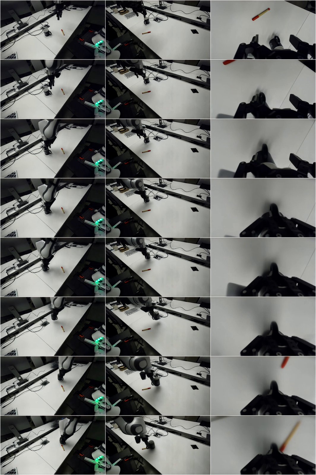
Figure 17: High Resolution 720p World Model Imagination Rollout.
图 17:高分辨率 720p 世界模型想象滚动。
Appendix E Qualitative World-Model Imagination Examples
附录 E 定性世界模型想象示例
Model-size comparison filmstrips. Each figure seeds RoboJEPA with the initial frame(s) of a held-out episode, replays the recorded actions, and shows the decoded imagination for every model size ( M– B) alongside the ground-truth (GT) video. Rows are ordered smallest-to-largest with GT at the bottom, directly beneath the B model for the most direct comparison; each row is sampled at k = 5 equal-time columns spanning the first s of the rollout. Big figures are decoded at the 480 × 640 encoder resolution and small at 240 × 320 ; the number of camera views is fixed per embodiment.
模型规模对比胶片条。每张图用保留回合的初始帧播种 RoboJEPA,重放记录动作,并展示每一模型规模(M–B)的解码想象,并排真实(GT)视频。行从小到大排列,GT 在底行、紧挨 B,便于直接对比;每行在滚动前 秒上等间隔采样 列。大图在编码器分辨率 解码,小图在 ;相机视角数按本体固定。
E.1 Large resolution (480 × 640 )
E.1 大分辨率()
Figures 18, 19, 20 and 21 show high-resolution rollouts on AgiBot, Bridge, and RoboCasa with one or two camera views.
图 18、19、20 与 21 展示 AgiBot、Bridge 与 RoboCasa 上单视角或双视角的高分辨率滚动。
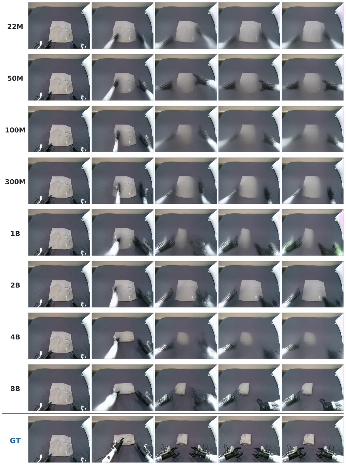
Figure 18: AgiBot (single view), 480 × 640 . Model-size comparison of world-model imaginations against ground truth; folding structure emerges only at larger scales.
图 18:AgiBot(单视角),。世界模型想象与真实的模型规模对比;折叠结构仅在较大规模出现。
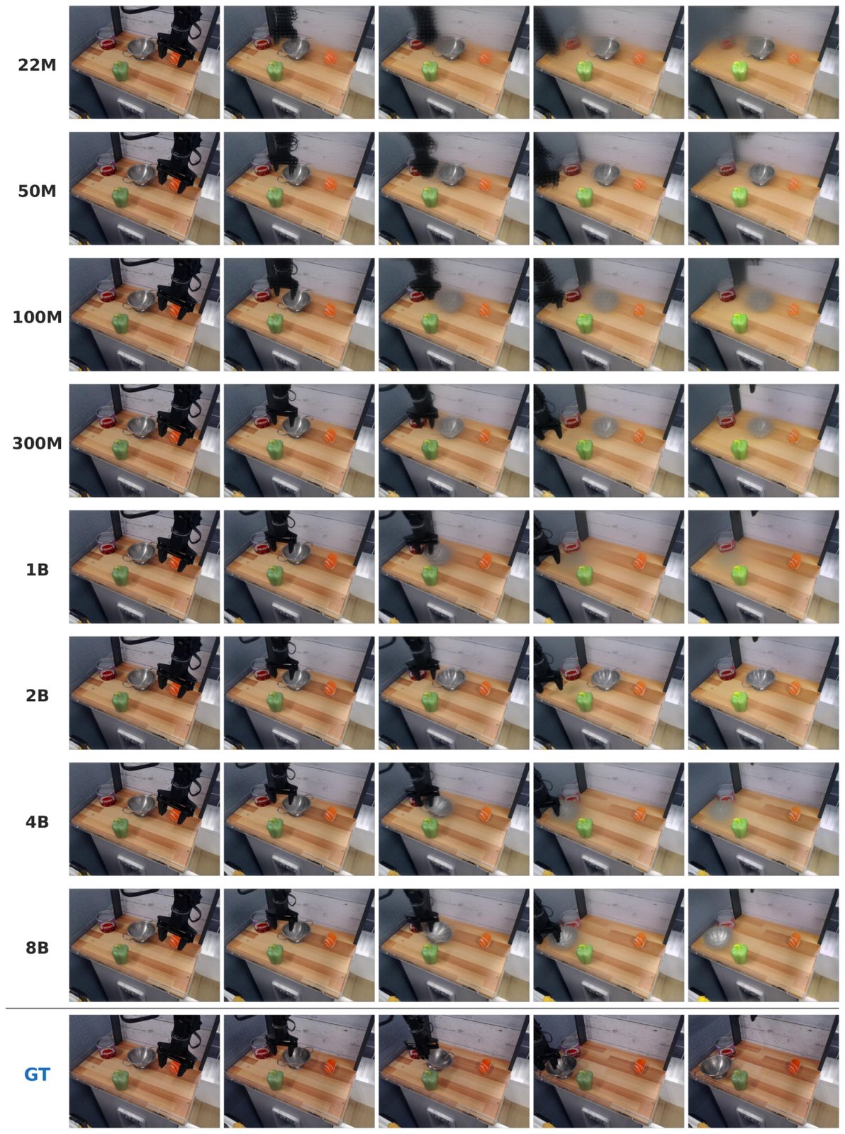
Figure 19: Open X-Embodiment Bridge (single view), 480 × 640 . Physical contact between the gripper and the object develops only for the larger models.
图 19:Open X-Embodiment Bridge(单视角),。夹爪与物体的物理接触仅在较大模型上形成。
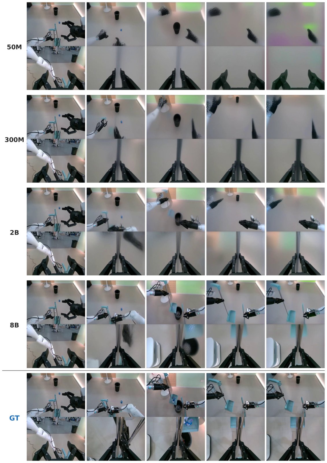
Figure 20: AgiBot (two views), 480 × 640 . Bimanual manipulation rollout across model sizes; finer details are preserved as scale increases.
图 20:AgiBot(双视角),。跨模型规模的双臂操作滚动;细节随规模增大而保留。
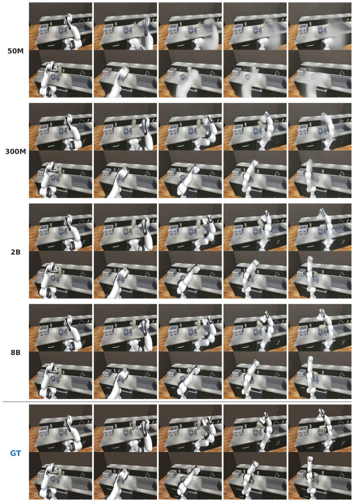
Figure 21: RoboCasa (two views), 480 × 640 . Simulated kitchen manipulation rollout across model sizes.
图 21:RoboCasa(双视角),。跨模型规模的仿真厨房操作滚动。
E.2 Small resolution (240 × 320 )
E.2 小分辨率()
Figures 22, 23, 24 and 25 show low-resolution rollouts on Bridge, Bridge V2, LeRobot, and DROID.
图 22、23、24 与 25 展示 Bridge、Bridge V2、LeRobot 与 DROID 上的低分辨率滚动。
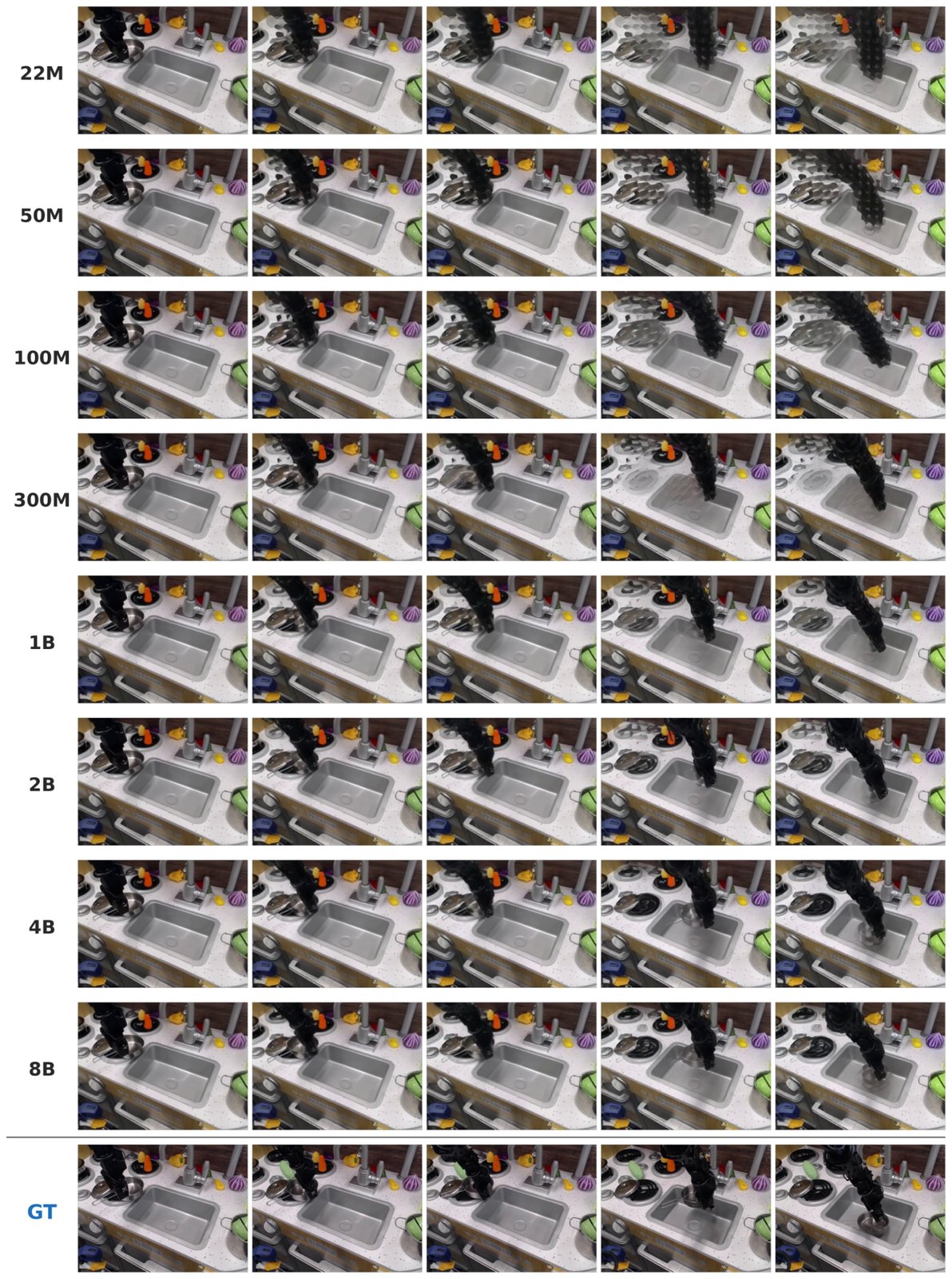
Figure 22: Open X-Embodiment Bridge (single view), 240 × 320 . Contact with the manipulated object develops only in the larger models.
图 22:Open X-Embodiment Bridge(单视角),。与被操作物体的接触仅在较大模型上形成。
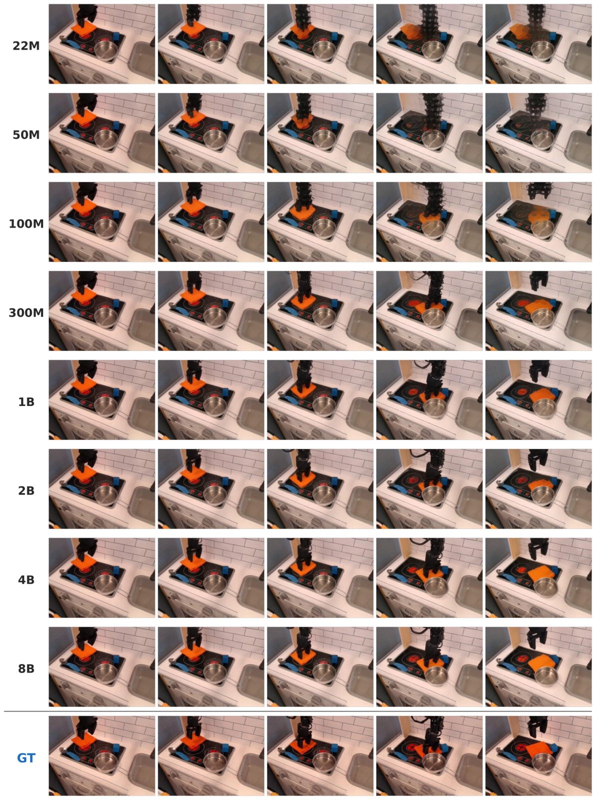
Figure 23: Bridge-V2 (single view), 240 × 320 . Clear progression of imagination quality with model scale.
图 23:Bridge-V2(单视角),。想象质量随模型规模清晰提升。
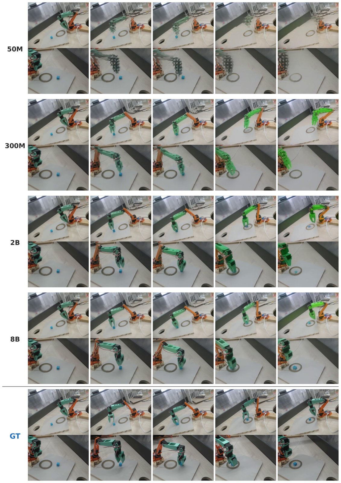
Figure 24: LeRobot (two views), 240 × 320 . Two-view manipulation rollout across model sizes.
图 24:LeRobot(双视角),。跨模型规模的双视角操作滚动。
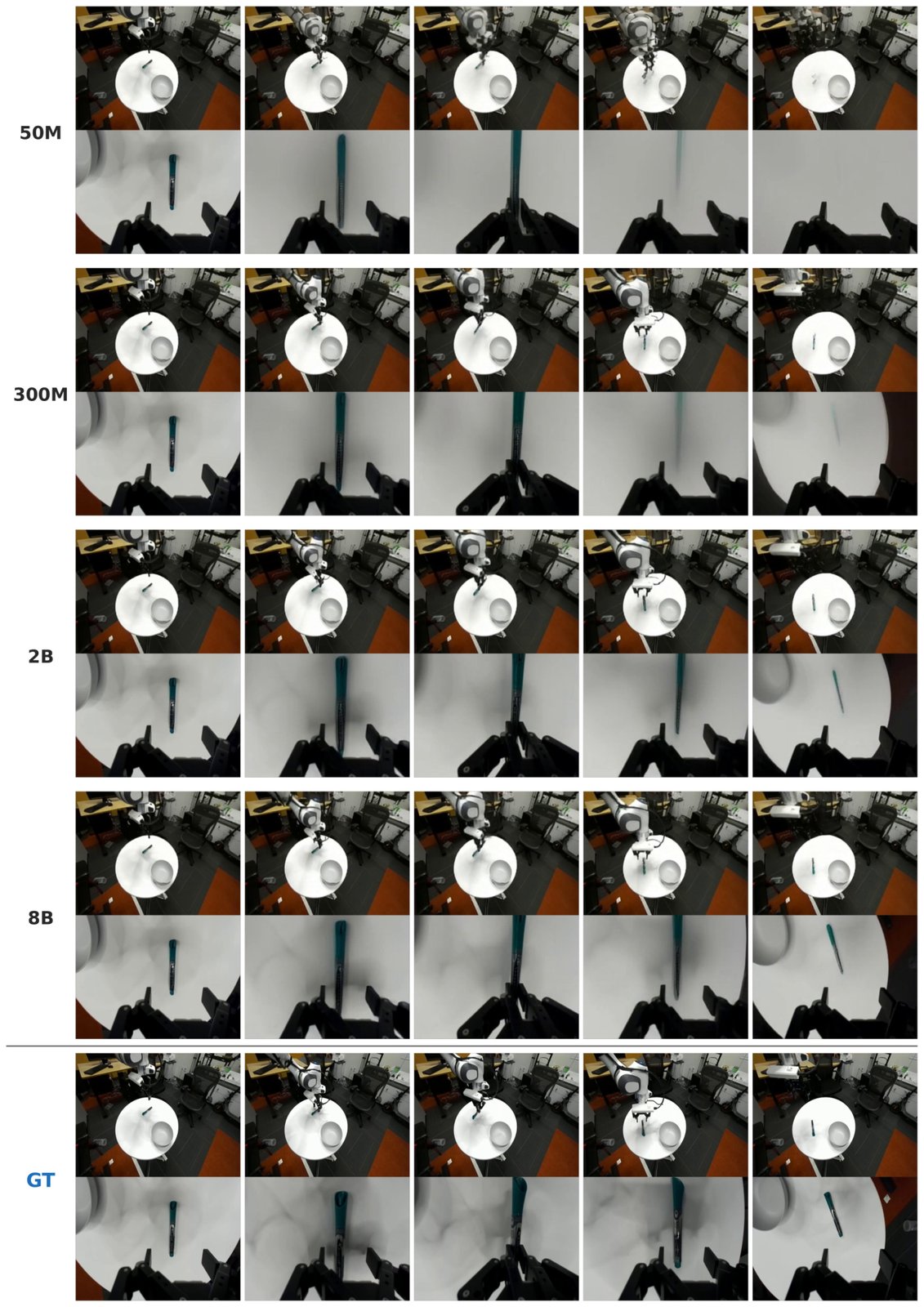
Figure 25: Franka / DROID (two views), 240 × 320 , joint-space actions. Two-view manipulation rollout across model sizes.
图 25:Franka / DROID(双视角),,关节空间动作。跨模型规模的双视角操作滚动。
Appendix F Planning: Additional Details
附录 F 规划:补充细节
Expands Section 2.2. We give the full algorithm box (Section F.1), the data-parallel elite selection (Section F.2), the spherical translation-sampling distribution (Section F.3), the ℓ 2 -ball projection (Section F.4), and multi-view goal handling (Section F.5). The computational cost of Equation 3 matches the per-token training loss (Section 2.2, Equation 5) and the controller-rate bridge (Section B.6) is what carries the planner output to the robot.
扩展第 2.2 节。我们给出完整算法框(F.1)、数据并行精英选择(F.2)、球坐标平移采样分布(F.3)、 球投影(F.4)以及多视角目标处理(F.5)。式 3 的计算代价与逐词元训练损失(第 2.2 节式 5)匹配;控制器速率桥(B.6)把规划器输出送到机器人。
F.1 Full CEM algorithm
F.1 完整 CEM 算法
Algorithm 1 restates one call to CEM with all loop details the main text suppressed. It exposes the per-iteration micro-batch loop ( micro-batches per GPU), the cross-rank AllGather, the explicit per-step return accumulation R (n) = ∑ h r h (n) , and the momentum-smoothed Gaussian refit. Across consecutive environment steps the planner is warm-started by shifting the previous mean by L exec steps and re-using its tail, so it converges in only I step refinement iterations after the cold-start computational cost of I 0 .
算法 1 重述一次 CEM 调用,补齐正文省略的循环细节。它暴露逐迭代微批循环(每 GPU 个微批)、跨秩 AllGather、显式逐步回报累积 ,以及动量平滑的高斯重拟合。跨连续环境步,规划器用前一均值平移 步并复用尾部做热启动,因而在冷启动代价 之后,只需 次精炼迭代即可收敛。
Algorithm 1 Receding-horizon CEM planning in V-JEPA feature space (full version).
算法 1:V-JEPA 特征空间中的后退地平 CEM 规划(完整版)。
F.2 Distributed elite selection
F.2 分布式精英选择
The planner is sharded data-parallel across GPUs: every rank draws its own N samp samples per refinement iteration and rolls them through its replica of g θ , using the same shared KV cache trick along the sample axis as on a single GPU. The per-rank rewards and the matching action tensors are then AllGather -ed (line 17 of Algorithm 1) so that every rank sees the same global pool of size N samp × G and can pick the top- elites independently and consistently. Because this elite set is selected from the global pool, the elite count is decoupled from the per-GPU sample count: in our DROID configuration we use N samp = 16 samples per GPU but k = 20 elites, which would be ill-defined on a single rank but is in fact a k = 20 out of a pool of N samp ⋅ G (≥ 256 in our deployments).
规划器在 块 GPU 上按数据并行分片:每秩在每次精炼迭代各自抽取 个样本,并用其 副本滚动,沿样本轴复用与单 GPU 相同的共享 KV 缓存技巧。然后 AllGather 逐秩奖励与匹配动作张量(算法 1 第 17 行),使每秩看到同一全局池 ,并独立且一致地选出 top- 精英。因精英集取自全局池, 与每 GPU 样本数解耦:我们的 DROID 配置每 GPU 样本但 精英——在单秩上本无定义,实为从池 (部署中 )中取 。
F.3 Spherical translation sampling
F.3 球坐标平移采样
Within each refinement iteration the proposal mean and standard deviation are per-step Gaussian, but we deviate from a vanilla isotropic Gaussian for the 3-D translation block. Following V-JEPA 2-AC (Assran et al., 2025), we draw the unit translation sample u ~ ∈ ℝ 3 from the joint density
每次精炼迭代内,提议均值与标准差是逐步高斯,但对三维平移块我们偏离朴素各向同性高斯。遵循 V-JEPA 2-AC(Assran 等,2025),从联合密度抽取单位平移样本
F.4 Translation ℓ 2 -ball projection
F.4 平移 球投影
After the affine warp a h (n) = μ h + σ h ⊙ a ~ h (n) , the translation block is projected onto an ℓ 2 -ball of radius ρ max that bounds the per-step end-effector displacement:
仿射变换 之后,平移块投影到半径 的 球上,以约束逐步末端位移:
F.5 Multi-view goal handling
F.5 多视角目标处理
When the world model is conditioned on multiple cameras, the computational cost in Equation 3 is summed across views with configurable per-view weights w v , re-using the per-block view conditioning of Section A.2 so that goal patches are compared at the correct viewpoint. Goal images that are unavailable for some views are handled by zeroing the corresponding w v at runtime, which lets us re-use the same multi-view checkpoint for single-camera DROID episodes without any retraining.
当世界模型以多路相机为条件时,式 3 的计算代价按可配置逐视角权重 跨视角求和,并复用 A.2 的逐块视角条件,使目标补丁在正确视点比较。某些视角缺失目标图像时,运行时将对应 置零,从而可把同一多视角检查点复用于单相机 DROID 回合而无需再训练。
Appendix G Robotic Setup
附录 G 机器人实验设置
G.1 Franka: DROID Platform
G.1 Franka:DROID 平台
Our real-robot experiments run on a Franka Panda arm with a parallel-jaw gripper, controlled through the original DROID software stack (Khazatsky et al., 2024). Deployment is split across two machines. A robot-control server runs on the robot PC and exposes the arm and cameras through a simple TCP/ZMQ request–reply interface; the planner client runs on a GPU cluster and connects to this server remotely. This separation lets the planner marshal a large number of GPUs for parallel world-model inference — the CEM optimizer samples and scores thousands of candidate rollouts per step across the cluster — while a single client process is the only one that exchanges observations and actions with the physical robot (Section G.3).
真机实验在带平行夹爪的 Franka Panda 臂上运行,经原始 DROID 软件栈控制(Khazatsky 等,2024)。部署跨两台机器:机器人控制服务器跑在机器人 PC 上,经简单 TCP/ZMQ 请求–应答接口暴露臂与相机;规划器客户端跑在 GPU 集群并远程连接该服务器。这种分离使规划器可调度大量 GPU 做并行世界模型推理——CEM 优化器每步在集群上采样并打分数千候选滚动——而只有单一客户端进程与物理机器人交换观测与动作(G.3)。
The scene is observed by two cameras: one ZED camera mounted on the wrist and one Intel RealSense camera placed externally to the left of the workspace (unlike the multi-ZED upstream DROID rig, we do not use a third camera). The wrist ZED records at 720 × 1280 and the external RealSense at 480 × 640 ; both streams are converted to RGB and resized to each agent’s native input resolution (240 × 320 for the RoboJEPA models) before encoding. At deployment RoboJEPA uses the resulting two views — external (left) and wrist.
场景由两路相机观察:腕部安装的 ZED,以及工作区左侧外置的 Intel RealSense(不同于上游多 ZED 的 DROID 机架,我们不用第三路)。腕部 ZED 录制 ,外置 RealSense 为 ;两路均转 RGB 并缩放到各智能体原生输入分辨率(RoboJEPA 模型为 )再编码。部署时 RoboJEPA 使用所得两视角——外置(左)与腕部。
For RoboJEPA we drive the robot with blocking end-effector control rather than a fixed-rate stream: each environment step commands an end-effector delta pose and then waits until the arm and gripper reach the commanded target before the next observation is returned, so the loop is paced by motion completion rather than a fixed control frequency. Although the underlying environment supports the full DROID action interface (7-DoF Cartesian and 8-DoF joint spaces, in velocity or position mode), our planner acts in a reduced space: it plans only D end-effector translation together with a D gripper command, holding the end-effector orientation fixed. The proprioceptive state we read back is the end-effector pose and gripper opening (with joint angles also available). At each step the planner encodes the current views and state into the world-model latent space, chooses an action by imagining short rollouts and scoring them against a goal image (Section 2.2), executes it, and repeats; each episode begins by homing the arm and recording the goal observation that defines the task. The full planning configuration is given in Section G.3.
对 RoboJEPA,我们用阻塞式末端控制而非固定速率流:每个环境步下达末端差分位姿,然后等到臂与夹爪到达目标才返回下一观测,因而环路由运动完成而非固定控制频率驱动。尽管底层环境支持完整 DROID 动作接口(笛卡尔 维与关节 维,速度或位置模式),我们的规划器在缩减空间动作:只规划 维末端平移加 维夹爪指令,末端朝向固定。读回的本体状态为末端位姿与夹爪开合(关节角亦可)。每步规划器把当前视角与状态编码到世界模型潜空间,通过想象短滚动并对齐目标图像打分选择动作(第 2.2 节),执行后重复;每回合先回零并记录定义任务的目标观测。完整规划配置见 G.3。
For baseline policies such as π 0.5 (Black et al., 2025) we instead use the standard DROID setup: non-blocking control at Hz in the joint-velocity action space, matching the interface these models were trained for.
对基线策略如 (Black 等,2025),我们改用标准 DROID 设置:关节速度动作空间上 Hz 非阻塞控制,以匹配这些模型的训练接口。

Figure 26: Real-world Franka lift the cup task. A goal image (left) and the initial observation (right) for one episode on the DROID/Franka platform, shown from both cameras: the external side camera (top) and the wrist-mounted camera (bottom). The task is specified purely by the goal image, in which the cup has been lifted off the table; from the start state the planner drives the world model toward these goal features. The two camera views are the inputs the world model is conditioned on at deployment.
图 26:真机 Franka「举起杯子」任务。DROID/Franka 平台上一回合的目标图像(左)与初始观测(右),两路相机:外置侧视(上)与腕部(下)。任务纯由目标图像指定——杯已离桌;从起始状态规划器驱动世界模型朝这些目标特征前进。两路相机视角是部署时世界模型的条件输入。
G.2 Real-robot tasks and evaluation protocol
G.2 真机任务与评测协议
Tasks and success criteria.
任务与成功标准。
We evaluate three tasks on the Franka/DROID platform: Grasp, Object Lift, and Pick and Place. Grasp requires the robot to grasp the object. Object Lift requires the robot to hold the object lifted in the air until the end of the episode. Pick and Place requires the object to end up at the target position, regardless of how many times it was dropped during the episode. These completion criteria do not imply one another: success on Pick and Place does not require satisfying the Object Lift criterion. Goal and initial observations for all three tasks are shown in Section G.6.
我们在 Franka/DROID 平台评测三项任务:Grasp、Object Lift 与 Pick and Place。Grasp 要求机器人抓住物体;Object Lift 要求回合结束前持续把物体举在空中;Pick and Place 要求物体最终落在目标位置,不论中途掉落几次。这些完成标准互不蕴含:Pick and Place 成功不必满足 Object Lift。三任务的目标与初始观测见 G.6。
Evaluation protocol.
评测协议。
For each model–task combination, we run episodes for RoboJEPA and episodes for each VLA baseline. We evaluate RoboJEPA models ranging from M to B parameters, using the checkpoint trained with the most compute at each size. All RoboJEPA models use the same planning hyperparameters across tasks, including the planning horizon. Hardware and controller details are provided in Section G.1, and the planning configuration is given in Section G.3.
对每个模型–任务组合,RoboJEPA 跑 回合,每个 VLA 基线跑 回合。评测 M 至 B 的 RoboJEPA 模型,各规模取算力最多的检查点。所有 RoboJEPA 模型跨任务使用相同规划超参(含规划地平)。硬件与控制器细节见 G.1,规划配置见 G.3。
For RoboJEPA, we generate a goal image by executing a predefined robot motion and manually placing the object in the grasping position so the robot can interact with it. Only the final image is provided as the goal for closed-loop planning; no intermediate image subgoals are used. The VLA baselines receive text instructions. Neither RoboJEPA nor the baselines receive task-specific fine-tuning.
对 RoboJEPA,我们执行预定义机器人运动并手动放置物体到可抓位置来生成目标图像。闭环规划只提供最终图像作为目标;不用中间图像子目标。VLA 基线接收文本指令。RoboJEPA 与基线均不做任务特定微调。
Scoring and reported metrics.
打分与报告指标。
We manually score each episode according to the task-specific completion criteria. For each model–task combination, we report task progress as the mean episode score and success rate as the fraction of episodes with 100 % progress. The per-model values are reported in Table 12.
我们按任务特定完成标准人工给每回合打分。对每个模型–任务组合,报告任务进度为平均回合得分,成功率为进度达 的回合比例。逐模型数值见表 12。
Table 12: Real-world robotic capabilities on the Franka/DROID platform. Task progress and success rate on the grasp, object-lift, and pick-and-place tasks. VLA baselines (π 0 -FAST and π 0.5 ) are conditioned on a text instruction, whereas all RoboJEPA models are conditioned on a single image goal.
表 12:Franka/DROID 平台真机机器人能力。抓取、举物与抓放任务上的任务进度与成功率。VLA 基线(-FAST 与 )以文本指令为条件,而所有 RoboJEPA 模型以单张目标图像为条件。
G.3 Real robot planning hyperparameters
G.3 真机规划超参
On the DROID/Franka platform the world model is deployed with the closed-loop CEM planner of Section 2.2 (full algorithm in Algorithm 1). The planner searches only over D end-effector translation and a D gripper command (rotation frozen), scores imagined rollouts by per-token ℓ 1 distance to the goal features in LN 0 space, and applies L exec actions per replan before re-observing. Table 13 lists the configuration used for all real-robot experiments.
在 DROID/Franka 平台上,世界模型配以第 2.2 节闭环 CEM 规划器部署(完整算法见算法 1)。规划器只搜索 维末端平移与 维夹爪指令(旋转冻结),在 空间用逐词元 距离对目标特征打分想象滚动,并在每次重规划前施加 个动作再重观测。表 13 列出全部真机实验所用配置。
Table 13: Closed-loop CEM planning hyperparameters for the DROID/Franka real-robot deployment (Section 2.2, Algorithm 1). Elites are selected from the pooled N samp ⋅ G samples gathered across the planner GPUs, so may exceed the per-GPU sample count. The planner acts in a D-translation + D-gripper space with the end-effector orientation held fixed.
表 13:DROID/Franka 真机部署的闭环 CEM 规划超参(第 2.2 节,算法 1)。精英从跨 块规划 GPU 汇集的 样本池选出,因而 可超过每 GPU 样本数。规划器在 维平移 + 维夹爪空间动作,末端朝向固定。
G.4 RoboCasa Custom Environments
G.4 RoboCasa 自定义环境
Our simulated evaluations use four custom tasks built on top of RoboCasa kitchen scenes (Nasiriany et al., 2024; Nasiriany et al., 2026) with the mobile-base PandaOmron (Franka Panda) robot. The four tasks share the same common controller. We drive the robot with a blocking controller that we implement on top of the simulator: each planner action specifies a target end-effector offset, which the environment servos toward with operational-space control until it converges (or a step cap is reached) before returning the next observation. We further extend the controller to drive the commanded end-effector rotation to convergence: rather than the default operational-space controller, which does not guarantee the orientation reaches its target, our controller feeds back the world-frame rotation error at every sub-step and only terminates once both the position and rotation errors fall below tolerance. We found this rotation convergence to be important for correctly matching the wrist-camera view during planning, since the planner scores candidates by a distance induced by both the side-view and the wrist-view predictions and the wrist camera is rigidly mounted to the end-effector, so any residual orientation drift would misalign the wrist view. RoboCasa exposes a large collection of kitchens split into training and evaluation scenes; the world model is trained on the training kitchens and all four tasks are run in the held-out evaluation kitchens. Because the environment is fully simulated, we can define both the goal image and the reward directly inside it. Every episode is instantiated from up to ten held-out target kitchens (one per layout/style pair), with non-structural countertop appliances near the workspace hidden to reduce clutter. Observations are rendered at 480 × 640 from the agent-view and, when enabled, wrist cameras. In every task the reward is the normalized progress toward the goal, r t = max (0, 1 − ∥ x t − x goal ∥ / d 0) , where d 0 is the initial goal distance.
仿真评测使用建于 RoboCasa 厨房场景之上的四项自定义任务(Nasiriany 等,2024;Nasiriany 等,2026),机器人是移动底座 PandaOmron(Franka Panda)。四任务共享同一通用控制器。我们在仿真器上实现阻塞控制器:每个规划动作指定目标末端偏移,环境用操作空间控制伺服直至收敛(或达到步数上限)再返回下一观测。我们进一步扩展控制器使指令末端旋转也收敛:默认操作空间控制不保证朝向到达目标,我们的控制器在每个子步反馈世界系旋转误差,仅当位置与旋转误差均低于容差才终止。我们发现旋转收敛对规划时正确匹配腕部相机视角很重要,因为规划器同时用侧视与腕部预测诱导的距离打分,而腕部相机刚体固连于末端,残留朝向漂移会使腕部视角错位。RoboCasa 提供大量厨房,分为训练与评测场景;世界模型在训练厨房上训练,四任务均在保留评测厨房运行。因环境完全仿真,目标图像与奖励均可在环境内直接定义。每回合从最多十个保留目标厨房实例化(每种布局/风格一对),并隐藏工作区附近非结构台面电器以减杂乱。观测以 从智能体视角渲染,启用时含腕部相机。每任务奖励为朝向目标的归一化进度 ,其中 为初始目标距离。
Reach.
Reach。
The robot must move its end-effector from a randomly sampled start pose to a randomly sampled goal pose in the kitchen. We remove all objects from the scene so that nothing occludes the path from the start to the goal. Start and goal are drawn uniformly within a small ball around the robot’s home pose and rejection-sampled so that they lie a fixed distance apart ( – m) and are reachable without a large reorientation of the end-effector. This task isolates the world model’s ability to predict free-space end-effector motion across kitchens. Figure 27 shows example goal and initial observations.
机器人须把末端从随机采样的起始位姿移到厨房中随机采样的目标位姿。我们清空场景中全部物体,使起终点路径无遮挡。起终点在机器人回零位姿附近小球内均匀抽取,并经拒绝采样使二者相距固定距离(– m)且无需大幅重定向即可到达。该任务隔离世界模型跨厨房预测自由空间末端运动的能力。图 27 给出示例目标与初始观测。

Figure 27: RoboCasa Reach. Goal and initial observations for one Reach episode, from the external side camera (top) and the wrist camera (bottom). The goal image (left) specifies the target end-effector pose in an emptied kitchen; the planner drives the arm from the start (right) toward the goal.
图 27:RoboCasa Reach。一回合 Reach 的目标与初始观测,外置侧视(上)与腕部(下)。目标图像(左)在清空厨房中指定目标末端位姿;规划器从起始(右)驱动臂朝目标前进。
ObstacleReach.
ObstacleReach。
A harder variant of Reach: one appliance (by default a coffee machine) is kept in the scene and repositioned directly in front of the robot, and the start and goal are constrained to lie on opposite sides of it. The end-effector must therefore arc around the obstacle rather than travel in a straight line, and the reachable distance band is widened ( – m). It tests whether the planner can find collision-free trajectories through the world model. Figure 28 shows an example episode.
Reach 的更难变体:场景保留一件电器(默认咖啡机)并直接放在机器人前方,起终点约束在其两侧。因而末端须绕障弧线运动而非直线,可达距离带加宽(– m)。检验规划器能否经世界模型找到无碰撞轨迹。图 28 给出示例回合。

Figure 28: RoboCasa ObstacleReach. Goal and initial observations for one ObstacleReach episode. An appliance placed directly in front of the robot forces the end-effector to arc around it, so the straight-line path from the start (right) to the goal (left) is blocked.
图 28:RoboCasa ObstacleReach。一回合 ObstacleReach 的目标与初始观测。电器正放在机器人前方,迫使末端绕行,因而从起始(右)到目标(左)的直线路径被挡住。
ObjectReach.
ObjectReach。
Here the robot must perform a reach while holding an object. To set this up, we first grasp the object with a heuristic scripted agent: a small Python controller that executes a top-down grasp (approach, descend, close, and lift) inside the simulator. Running the grasp in simulation ensures the object is held in a physically correct way before planning begins. The world model then has to move the held object to a randomly sampled goal position, and the reward is the normalized progress of the object toward its goal rather than of the end-effector. The object is one of a banana, a can, or a mug, which differ in shape and physical properties (friction and grasp offsets are tuned per object). Figures 29, 30 and 31 show examples for the three objects.
此处机器人须在持物状态下完成到达。为此我们先用启发式脚本智能体抓取物体:仿真内执行自上而下抓取(接近、下降、闭合、抬起)的小型 Python 控制器。在仿真中跑抓取可确保规划开始前物体以物理正确方式被持住。随后世界模型须把所持物体移到随机采样目标位置,奖励是物体而非末端朝目标的归一化进度。物体为香蕉、罐头或马克杯之一,形状与物理属性不同(摩擦与抓取偏移按物体调)。图 29、30、31 给出三物体示例。

Figure 29: RoboCasa ObjectReach (banana). Goal and initial observations after the scripted grasp: from the start (right) the robot must carry the held banana to the goal pose (left), shown from the side (top) and wrist (bottom) cameras.
图 29:RoboCasa ObjectReach(香蕉)。脚本抓取后的目标与初始观测:从起始(右)机器人须把所持香蕉带到目标位姿(左),侧视(上)与腕部(下)。

Figure 30: RoboCasa ObjectReach (can). As in Figure 29 for the can object.
图 30:RoboCasa ObjectReach(罐头)。同图 29,对象为罐头。

Figure 31: RoboCasa ObjectReach (mug). As in Figure 29 for the mug object.
图 31:RoboCasa ObjectReach(马克杯)。同图 29,对象为马克杯。
ObjectPush.
ObjectPush。
The robot must push the object across the counter by contact from a randomly sampled start position to a randomly sampled goal position. The gripper is held closed so that it acts as a solid pusher, and the arm is driven by translation deltas, so the object moves only through contact rather than being grasped. Start and goal are sampled a fixed distance apart ( – m) within a small disk on the counter; because forward pushes (along the robot’s reach direction) are far more reliable than lateral ones, the push direction is restricted to a 60 ∘ cone around the forward axis. As in ObjectReach, the reward is the normalized progress of the object toward its goal. This task probes whether the world model captures non-prehensile, contact-rich dynamics. Figure 32 shows example goal and initial observations.
机器人须通过接触把物体从随机起始位置推过台面到随机目标位置。夹爪保持闭合以充当刚性推杆,臂由平移差分驱动,因而物体只经接触移动而非被抓取。起终点在台面小圆盘内相距固定距离(– m)采样;因沿机器人伸展方向的前推远比侧推可靠,推动方向限制在前向轴周围 锥内。与 ObjectReach 一样,奖励是物体朝目标的归一化进度。该任务探查世界模型是否捕获非抓取、富接触动力学。图 32 给出示例目标与初始观测。

Figure 32: RoboCasa Push. Goal and initial observations for one object-push episode, shown from the side (top) and wrist (bottom) cameras. The robot must push the object across the counter from its initial position (right) to the goal position (left). Note that the goal pose and the initial pose of the robot are the same, the only thing that changes is the object position.
图 32:RoboCasa Push。一回合物体推动的目标与初始观测,侧视(上)与腕部(下)。机器人须把物体从初始位置(右)推到目标位置(左)。注意目标位姿与机器人初始位姿相同,唯一变化的是物体位置。
G.5 RoboCasa planning hyperparameters
G.5 RoboCasa 规划超参
All four RoboCasa tasks are solved with the same closed-loop CEM planner (Section 2.2, Algorithm 1). Across the four tasks the only CEM hyperparameter we vary is the predictor horizon ; every other CEM setting is shared (Table 14, top). Push uses the same planning configuration as ObstacleReach. As in the DROID configuration (Table 13) the planner scores rollouts by per-token ℓ 1 distance to the goal features and re-plans after every executed action. Reach and ObstacleReach and Push search over D end-effector translation, while ObjectReach first grasps an object with a scripted agent and then additionally searches the gripper. The tasks otherwise differ in their environment configuration (Table 14, bottom).
四项 RoboCasa 任务均用同一闭环 CEM 规划器求解(第 2.2 节,算法 1)。跨四任务我们唯一变动的 CEM 超参是预测器地平 ;其余 CEM 设置共享(表 14 上半)。Push 与 ObstacleReach 使用相同规划配置。与 DROID 配置(表 13)一样,规划器用逐词元 距离对目标特征打分滚动,并在每次执行动作后重规划。Reach、ObstacleReach 与 Push 搜索 维末端平移,而 ObjectReach 先由脚本智能体抓取物体,再额外搜索夹爪。任务在环境配置上另有差异(表 14 下半)。
Table 14: Planning and environment configuration for the four RoboCasa tasks (Section G.4). The table is split into the planning hyperparameters (top) and the environment parameters (bottom). Among the planning hyperparameters, only the predictor horizon varies across tasks; the rest are shared. The effective CEM sample budget is candidates per iteration for every task (distributed across the planner GPUs), from which the top- elites are selected.
表 14:四项 RoboCasa 任务的规划与环境配置(G.4)。表分为规划超参(上)与环境参数(下)。规划超参中仅预测器地平 跨任务变化;其余共享。有效 CEM 样本预算为每迭代 候选(分布在规划 GPU 上),并从中选出 top- 精英。
G.6 Real-Robot Task Examples
G.6 真机任务示例
Figures 33, 34 and 35 show goal and initial observations for Grasp, Object Lift, and Pick and Place, respectively. We show goal and initial observations for the three real-robot deployment tasks (grasp, lift, and pick-and-place), ten episodes each, from both the external side camera and the wrist camera. The goal is provided to the planner as a single image; recall that the goal and the initial robot pose coincide, so the visible difference between the goal and initial columns is the configuration of the manipulated object.
图 33、34、35 分别给出 Grasp、Object Lift 与 Pick and Place 的目标与初始观测。我们展示三项真机部署任务(抓取、举起、抓放)各十回合的目标与初始观测,含外置侧视与腕部相机。目标以单张图像提供给规划器;回顾目标与初始机器人位姿重合,因而目标列与初始列的可见差异是被操作物体的配置。
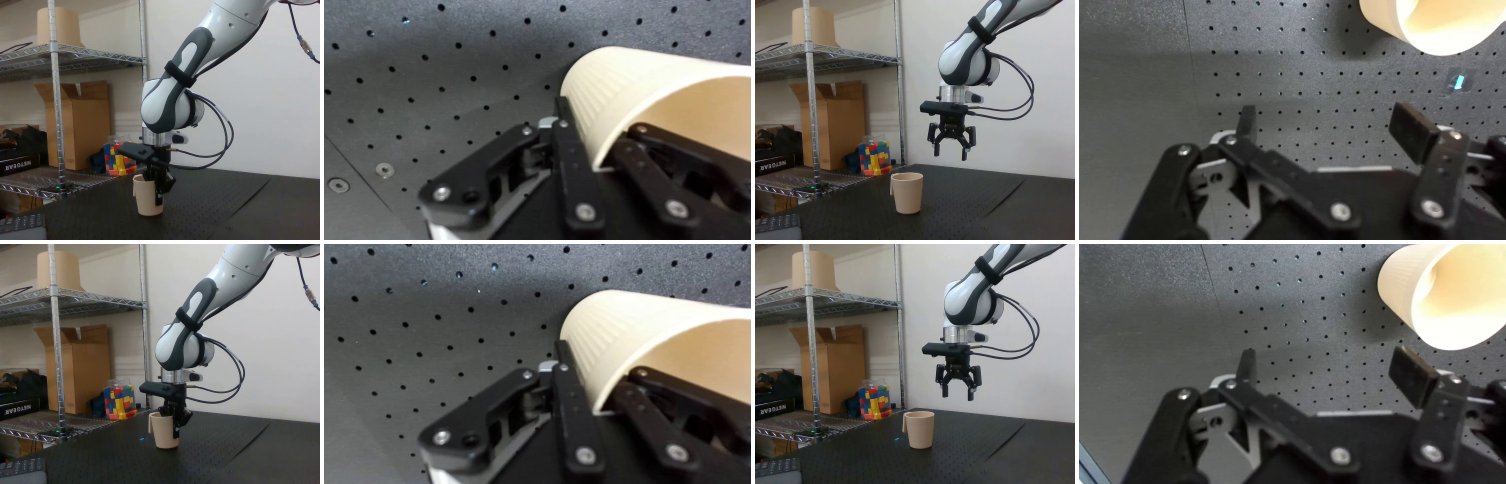
Figure 33: Real-robot Grasp task: goal and initial observations. Ten episodes (rows) of the Grasp task on the DROID/Franka platform. For each episode we show the goal image (left pair) and the initial state (right pair), each from the external side camera and the wrist camera. The goal is specified purely by these images; the planner drives the robot from the initial state toward the goal.
图 33:真机 Grasp 任务:目标与初始观测。DROID/Franka 平台 Grasp 任务十回合(行)。每回合展示目标图像(左对)与初始状态(右对),各含外置侧视与腕部。目标纯由这些图像指定;规划器从初始状态驱动机器人朝目标前进。
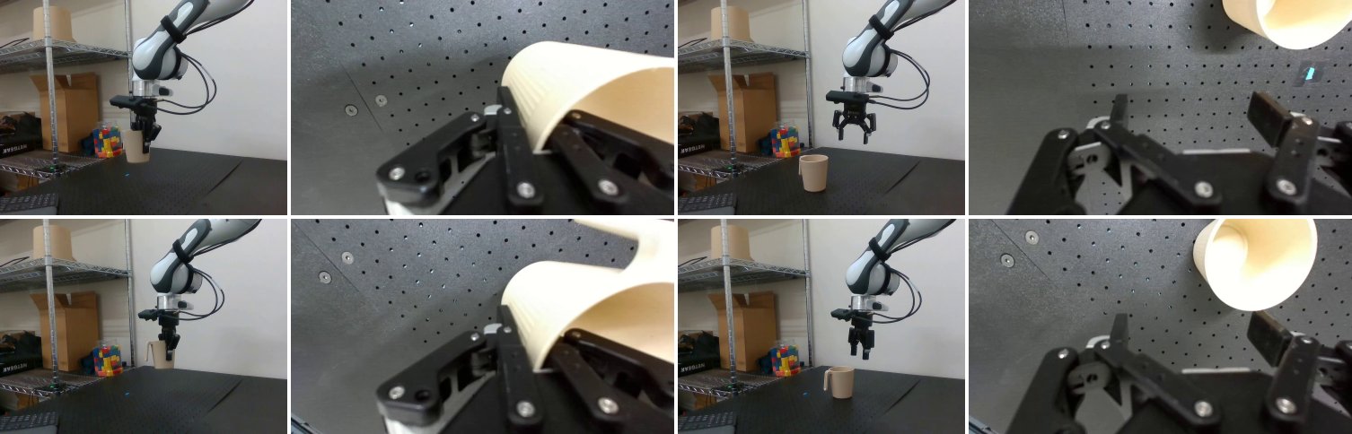
Figure 34: Real-robot Lift task: goal and initial observations. Ten episodes (rows) of the Lift task on the DROID/Franka platform. For each episode we show the goal image (left pair) and the initial state (right pair), each from the external side camera and the wrist camera. The goal is specified purely by these images; the planner drives the robot from the initial state toward the goal.
图 34:真机 Lift 任务:目标与初始观测。DROID/Franka 平台 Lift 任务十回合(行)。每回合展示目标图像(左对)与初始状态(右对),各含外置侧视与腕部。目标纯由这些图像指定;规划器从初始状态驱动机器人朝目标前进。
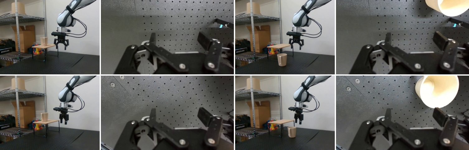
Figure 35: Real-robot Pick-and-Place task: goal and initial observations. Ten episodes (rows) of the Pick-and-Place task on the DROID/Franka platform. For each episode we show the goal image (left pair) and the initial state (right pair), each from the external side camera and the wrist camera. The goal is specified purely by these images; the planner drives the robot from the initial state toward the goal.
图 35:真机 Pick-and-Place 任务:目标与初始观测。DROID/Franka 平台 Pick-and-Place 任务十回合(行)。每回合展示目标图像(左对)与初始状态(右对),各含外置侧视与腕部。目标纯由这些图像指定;规划器从初始状态驱动机器人朝目标前进。
G.7 Real World Robotic Capabilities
G.7 真机机器人能力
We observe qualitative differences in the behavior induced by planning with small and large world models. Small models’ main weakness is poor gripper control, yet their successful episodes exhibit smooth end-effector trajectories and accurate approaches to objects. They struggle to recover after approaching an object from an unsuitable grasping position, whereas larger models can adapt and recover from such mistakes. As model size increases, behavior gradually shifts from smooth execution relying on a single grasping attempt toward more adaptive and robust execution. Intermediate models, such as the M and B variants, appear to lie between these behavioral regimes, combining some of the limitations of smaller models with emerging recovery capabilities.
我们观察到用小世界模型与大世界模型规划时行为的定性差异。小模型主要弱点是夹爪控制差,但其成功回合仍表现出平滑的末端轨迹与对物体的准确接近。它们难以从不当抓取位姿接近后恢复,而较大模型能适应并从这类错误中恢复。随模型增大,行为逐渐从依赖单次抓取尝试的平滑执行,转向更具适应与鲁棒性的执行。中间规模如 M 与 B 变体似乎介于两种行为体制之间,兼有小模型的部分局限与初现的恢复能力。
When comparing RoboJEPA with the VLA reference models, we cannot fully disentangle the contribution of image-goal specification from that of world-model scaling. The differences in training data and controller interfaces described in Section G.1 also limit this comparison. Nevertheless, all RoboJEPA model sizes use the same goal specification and planning configuration, and the observed improvement across sizes suggests that model scaling contributes to the capabilities of the resulting planner. These qualitative observations complement the task progress and success rates reported in Table 12.
将 RoboJEPA 与 VLA 参考模型比较时,我们无法完全拆开图像目标指定与世界模型缩放各自的贡献。G.1 所述训练数据与控制器接口差异也限制该比较。尽管如此,所有 RoboJEPA 模型规模使用相同目标指定与规划配置,跨规模观察到的提升表明模型缩放有助于所得规划器的能力。这些定性观察补充表 12 报告的任务进度与成功率。
Appendix H Key-Value Cache: Additional Details
附录 H 键值缓存:补充细节
For each predictor layer, we cache the keys and values of past timesteps so that autoregressive prediction processes only the new frame, action, and state tokens. Each timestep contains
对每个预测器层,我们缓存过去时间步的键与值,使自回归预测只处理新帧、动作与状态词元。每个时间步包含
As prediction advances, the rolling cache replaces the oldest frame with the new one. RoPE uses absolute timestep indices, so cached positions do not need to be renumbered when the buffer wraps. Each new frame attends only to the retained window, keeping the amount of cached history bounded even for long rollouts.
随预测推进,滚动缓存用新帧替换最旧帧。RoPE 使用绝对时间步索引,因而缓冲环绕时缓存位置无需重编号。每新帧只关注保留窗口,使即使长滚动缓存历史量仍有界。
At the start of each planning call, we process the observation context once and share its cached keys and values across the CEM candidates. Subsequent predictions maintain candidate-specific caches because their action sequences differ. This avoids repeatedly processing the same observation history, while each prediction step processes only the new tokens and attends to a fixed-size window of cached tokens. The compilation pipeline is described in Appendix I.
每次规划调用开始时,我们处理一次观测上下文,并跨 CEM 候选共享其缓存键值。后续预测维护候选特定缓存,因其动作序列不同。这避免重复处理同一观测历史,而每预测步只处理新词元并对固定大小缓存词元窗做注意力。编译管线见附录 I。
Appendix I Inference Engine: Additional Details
附录 I 推理引擎:补充细节
Expands Section 2.2. The story of the inference engine is one long descent: start from the V-JEPA 2-AC (Assran et al., 2025) eager BF16 baseline, identify what binds it (host-side dispatch, not arithmetic; Section I.1), unbind it with PyTorch Inductor lowering and ahead-of-time compilation that also makes cold start usable on a robot (Section I.2), then squeeze the remaining matmul time with a static FP8 path on top (Section I.3). Section I.4 records the roads we abandoned because the workload simply was not where they help. All numbers are wall-clock measurements on a single NVIDIA H200 (140 GB HBM3) running PyTorch 2.9, on the 1 B predictor at 240p with grouped-query attention (12 query heads, 4 KV heads, 40 layers, 1536 hidden dim), and the rolling KV cache of L cache = 8 frames.
扩展第 2.2 节。推理引擎的故事是一条长下坡:从 V-JEPA 2-AC(Assran 等,2025)的 eager BF16 基线出发,找出束缚它的是什么(主机侧调度,而非算术;I.1),用 PyTorch Inductor 降低与提前编译解绑,并使冷启动可在机器人上使用(I.2),再在其上用静态 FP8 路径挤出剩余 matmul 时间(I.3)。I.4 记录我们放弃的路径,因为工作负载并不在它们能帮到的地方。全部数字为单块 NVIDIA H200(140 GB HBM3)上跑 PyTorch 2.9 的墙钟测量,对象是 p 上带分组查询注意力的 1B 预测器( 查询头、 KV 头、 层、隐维 ),以及 帧的滚动 KV 缓存。
I.1 Where the time goes (why the model is not matmul-bound)
I.1 时间花在哪里(为何模型并非 matmul 受限)
Naive BF16 inference is bound by host-side dispatch, not by matrix multiplication.
朴素 BF16 推理受主机侧调度束缚,而非矩阵乘法。
At steady state (B = 16 , full KV cache, 2-view) GEMMs take only ∼ 26 % of GPU time, attention ∼ 41 % , and fused pointwise ops (RoPE, GELU, normalizations, cache management) the remaining ∼ 33 % ; on top of that, eager mode burns ∼ 31 % of wall time in dispatch overhead. Doubling GEMM throughput would buy at most a 1.21 × end-to-end factor; removing dispatch and fusing the long pointwise tail are the first-order wins. At B = 1 the same decomposition is even more dispatch-dominated (∼ 47 % of wall time), which is why the headline speedups in Section 2.2 are largest at small batch. Per-step kernel share within a single rollout is dominated by attention growing with cache occupancy: at step attention is ∼ 14 % of step time; at step ∼ 32 % ; at full cache (step 7 + ) ∼ 41 % . GEMM time stays roughly constant at ∼ 25 ms per step regardless of cache depth. This is the computational-cost picture that the rest of the engine targets.
稳态下(,满 KV 缓存,双视角)GEMM 仅占 GPU 时间 ,注意力 ,融合逐点算子(RoPE、GELU、归一化、缓存管理)占余下 ;此外 eager 模式把墙钟约 烧在调度开销上。把 GEMM 吞吐翻倍最多买到 端到端因子;去掉调度并融合长逐点尾巴才是一阶收益。在 时同一分解更受调度主导(墙钟 ),这正是第 2.2 节标题加速在小批量最大的原因。单次滚动内逐步核占比随缓存占用增长:步 注意力约 步时间;步 约 ;满缓存(步 )约 。GEMM 时间大致恒定在每步 ms,与缓存深度无关。这是引擎其余部分所针对的计算代价图景。
Table 15: Per-step decomposition into GPU kernel time and host-side dispatch overhead at B = 16 on H200. AOT Inductor removes essentially all dispatch (− 65 ms) and additionally speeds up GPU compute by ∼ 1.8 × through kernel fusion (8,975 → 1,291 kernels for the 1-view model). -view rows are retained here because dispatch behavior is qualitatively different at small sequence length, even though the deployed CEM planner runs the 2-view path.
表 15:H200 上 时逐步分解为 GPU 核时间与主机侧调度开销。AOT Inductor 几乎去掉全部调度( ms),并通过核融合额外把 GPU 计算加速约 (单视角模型 个核)。此处保留单视角行,因小序列长度下调度行为有质差异,尽管部署的 CEM 规划器跑双视角路径。
I.2 AOT Inductor compilation: from dispatch to deployment
I.2 AOT Inductor 编译:从调度到部署
The natural answer to dispatch overhead is to lower the per-step graph into fused Triton kernels with PyTorch Inductor (Ansel et al., 2024). A JIT torch.compile path does this, but it specializes into many shape variants on the first call; we measure – minutes of warm-up at robot start per autoregressive step pattern, which is incompatible with closed-loop deployment where the operator turns the robot on and expects it to plan in seconds.
对调度开销的自然回答是用 PyTorch Inductor(Ansel 等,2024)把逐步图降低为融合 Triton 核。JIT 的 torch.compile 路径能做到,但首次调用会特化出许多形状变体;我们测得每个自回归步模式在机器人启动时需预热 – 分钟,这与闭环部署不相容——操作员开机后期望几秒内开始规划。
Autoregressive predictor inference, however, has a small predictable shape set. At step with batch size , every tensor shape is fully determined; the rolling cache has only distinct configurations (steps – grow the cache; step overwrites the oldest entry and repeats forever). With six compiled batch sizes B ∈ { 1, 2, 4, 8, 16, 32 } this produces static programs for the predictor; the diffusion decoder of Section 2.3 compiles to an analogous family of programs through the same pipeline. Each program is exported with torch.export under static shapes and packaged via torch._inductor.aoti_compile_and_package into a – MB compiled C++ artefact.
然而自回归预测器推理有一组小且可预测的形状。在步 、批量 时,每个张量形状完全确定;滚动缓存只有 种不同配置(步 – 增长缓存;步 覆盖最旧条目并永远重复)。配合六个编译批量 ,预测器产生 个静态程序;第 2.3 节扩散解码器经同一管线编译为类似程序族。每个程序在静态形状下用 torch.export 导出,再经 torch._inductor.aoti_compile_and_package 打成 – MB 的已编译 C++ 产物。
The static-shape lowering has two prerequisites that drive engineering choices upstream. First, a mutation-free cache: torch.export ’s functionalisation rewrites in-place slices into hundreds of aten.copy ops, which inflated GPU buffer count by ∼ 5 × in our first pass. We thread a functional cache through every block (each block reads the input cache tensors and returns fresh ones, the per-layer outputs are stacked, and a wrapper module bakes cache_size and input_position as compile-time constants). The functional path produces bitwise-identical outputs to the in-place version across all cache regimes (empty, mid, full). Second, shared weight tensors across programs: because the ∼ GB BF16 weight set is held once rather than once per program, this drops resident memory from ∼ 108 GB to ∼ 14 GB — the difference between fitting and not fitting on the deployment box. Non-compiled batch sizes are padded up to the nearest compiled value (e.g. B = 3 → 4 ) and sliced back on output, so the worst-case waste from bucketing is ∼ 50 % when the requested is just above a compiled size.
静态形状降低有两项驱动上游工程选择的前提。其一,无突变缓存:torch.export 的函数化会把原地切片重写为数百 aten.copy,我们第一遍把 GPU 缓冲数胀了约 。我们把函数式缓存穿过每块(每块读入缓存张量并返回新张量,逐层输出堆叠,包装模块把 cache_size 与 input_position 烤成编译时常量)。函数式路径在全部缓存体制(空、中、满)上产生与原地版本逐位相同的输出。其二,跨程序共享权重张量:约 GB BF16 权集只持有一份而非每程序一份,常驻内存从约 GB 降到约 GB——决定能否装进部署机。未编译批量上取整到最近已编译值(如 )并在输出切回,因而分桶最坏浪费约 (当请求 刚好略高于已编译尺寸时)。
End-to-end the AOT pipeline yields a 7 × reduction in launched kernels (8, → 1,291 for the 1-view predictor), a 1.8 × GPU compute speedup from better fusion, and a 23 × reduction in dispatch overhead (Table 15). Crucially, cold start collapses from – minutes (JIT) to – seconds: the time to load the .pt2 files and inject the shared weights. The computational cost of offline compilation ( – minutes total, parallelised across multiple H200s by an offline compiler) is paid once per checkpoint; thereafter the runtime dispatcher loads the compiled archives and routes each step() call to the matching program. Inside the AOT pipeline we keep one positive low-level result that the failed-attempts ledger would otherwise hide: native GQA dispatched to FlashAttention (Dao et al., 2022; Dao, 2024) avoids the implicit repeat_interleave expansion that the cuDNN attention path uses, contributing the ∼ 3 % on top that survives in the headline recipe.
端到端 AOT 管线把启动核数降 (单视角预测器 ),因更好融合带来 GPU 计算加速,并把调度开销降 (表 15)。关键的是,冷启动从 JIT 的 – 分钟塌到 – 秒:加载 个 .pt2 文件并注入共享权重的时间。离线编译的计算代价(总计 – 分钟,由离线编译器跨多块 H200 并行)按检查点付一次;此后运行时调度器加载已编译归档,并把每次 step() 路由到匹配程序。在 AOT 管线内我们保留一项失败尝试账本本会掩盖的正面低层结果:原生 GQA 派发到 FlashAttention(Dao 等,2022;Dao,2024)避免 cuDNN 注意力路径所用的隐式 repeat_interleave 展开,贡献标题配方中仍存活的约 。
I.3 Static FP8 path: the last small lever
I.3 静态 FP8 路径:最后的小杠杆
After AOT removes dispatch, what remains is steady-state GEMM and attention time. We can shave a final factor by running the predictor’s linear layers in FP8. Because the workload is not matmul-bound, this is genuinely a small lever — which is itself the data point that justifies the engineering: order wins, not low-precision arithmetic. The FP8 path (Table 16) runs through torch.compile(fullgraph=True) rather than the AOTI path because the AOTI loader currently mishandles many co-resident FP8 programs; the JIT path with the Inductor disk cache is instant after the first compile. Activation scales are calibrated once on a small held-out set and stored as fixed buffers; weights are kept as float8_e4m3fn with fast-accumulate FP8 GEMMs. Outputs match the BF16 reference to within the spatial-sensitivity benchmark’s noise floor (Section 3.2). Table 16 reports per-cache-step latency at B = 16 on the 2-view model: the FP8 advantage is largest at low cache occupancy where the GEMM share is relatively higher; once attention dominates at full cache it shrinks to ∼ 5 % .
AOT 去掉调度后,剩下的是稳态 GEMM 与注意力时间。我们可通过以 FP8 跑预测器线性层再削一个最终因子。因工作负载并非 matmul 受限,这确实是小杠杆——而这本身就是证明工程合理性的数据点:顺序优先,而非低精度算术。FP8 路径(表 16)经 torch.compile(fullgraph=True) 而非 AOTI 路径,因 AOTI 加载器目前对许多共存 FP8 程序处理不当;带 Inductor 磁盘缓存的 JIT 路径在首次编译后瞬时。激活尺度在小保留集上校准一次并存为固定缓冲;权重保持 float8_e4m3fn 并用快速累加 FP8 GEMM。输出与 BF16 参考在空间敏感基准的噪声底内一致(第 3.2 节)。表 16 报告双视角模型 时逐步缓存延迟:FP8 优势在低缓存占用(GEMM 份额相对更高)时最大;满缓存注意力主导后缩至约 。
Table 16: Static FP8 vs. BF16 AOTI on the 2-view 1B predictor at B = 16 , averaged across the rolling-cache trajectory.
表 16:双视角 1B 预测器在 上静态 FP8 与 BF16 AOTI 对比,沿滚动缓存轨迹平均。
I.4 Optimisations that did not work
I.4 未奏效的优化
We document the negative results because they sharpen the picture of what the dominant computational cost actually is.
我们记录负面结果,因为它们能锐化主导计算代价究竟是什么的图景。
Dynamic FP8.
动态 FP8。
A first FP8 attempt with per-call activation amax computation was slower than BF16 ( ms vs. ∼ 100 ms): the three extra ops per linear (cast to FP32, amax reduction, quantise) have a higher computational cost than the FP8 GEMM saves on a model that is not matmul-bound. Static, pre-calibrated scales (Section I.3) eliminate this overhead.
首次带逐调用激活 amax 计算的 FP8 尝试慢于 BF16( ms 对约 ms):每个线性多出的三个算子(转 FP32、amax 归约、量化)的计算代价高于 FP8 GEMM 在非 matmul 受限模型上的节省。静态预校准尺度(I.3)消除该开销。
Weight-only INT8 and W8A8 / F8A8 variants.
仅权重 INT8 与 W8A8 / F8A8 变体。
The torchao implementations were either incompatible with the dispatcher’s requirement that linear outputs match the BF16 KV-cache dtype required by FlashAttention, or produced ∼ 2 × slower forwards because dequantisation overhead dominates on a compute-bound (not bandwidth-bound) model.
torchao 实现要么与调度器要求线性输出匹配 FlashAttention 所需 BF16 KV 缓存 dtype 不兼容,要么因去量化开销在计算受限(非带宽受限)模型上主导而产生约 更慢的前向。
CUDA graphs.
CUDA graphs。
Reduce-overhead capture segfaults inside the captured graph because the KV cache slice assignment mutates a GPU tensor whose target offset changes between replays. A clone-based workaround runs but is slower ( ms vs. ms) than the non-graph path: once AOT has reduced dispatch overhead to ∼ 3 ms there is essentially nothing left for graph capture to amortise.
减开销捕获在捕获图内段错误,因 KV 缓存切片赋值突变 GPU 张量,且目标偏移在重放间变化。基于 clone 的变通能跑但慢于非图路径( ms 对 ms):一旦 AOT 把调度开销降到约 ms,图捕获几乎无可摊销之物。
TensorRT.
TensorRT。
Both whole-model and per-block TensorRT wrappers were slower ( – 0.7 × ) and produced incorrect outputs, tripping a known multi-output-export bug. AOT Inductor already produces near-optimal fused Triton kernels for this architecture, so TensorRT did not add value.
整模与逐块 TensorRT 包装均更慢(–)并产生错误输出,触发已知多输出导出 bug。AOT Inductor 已为该架构产生近最优融合 Triton 核,因而 TensorRT 未增加价值。
RoPE pre-computation.
RoPE 预计算。
Pre-computing cos/sin tables as registered buffers gave 0 % speedup under AOT, because Inductor already fuses RoPE inline into its surrounding Triton kernels.
把 cos/sin 表预计算为注册缓冲在 AOT 下加速 ,因为 Inductor 已把 RoPE 内联融合进周围 Triton 核。
cuDNN attention in AOT.
AOT 中的 cuDNN 注意力。
sdpa_cudnn is 2.4 × faster than xformers_fmha in isolation but only ∼ 3 % faster in the AOT pipeline: torch.export captures all SDPA variants as the same ATen op and AOT Inductor lowers to flash-attention regardless of context-manager hint. The native-GQA-without- repeat_interleave factor that survives is reported as part of the AOT pipeline (Section I.2).
孤立看 sdpa_cudnn 比 xformers_fmha 快 ,但在 AOT 管线中仅快约 :torch.export 把所有 SDPA 变体捕获为同一 ATen 算子,且不论上下文管理器提示,AOT Inductor 都降到 flash-attention。存活的「原生 GQA、无 repeat_interleave」因子作为 AOT 管线一部分报告(I.2)。
Appendix J Scaling Laws: Additional Parametric Forms
附录 J 缩放律:额外参数形式
Expands Section 3.1 and Table 2. In addition to the saturating power law and the second-order power law of Section 3.1, we fit two published functional forms as extrapolation baselines: the Broken Neural Scaling Law (BNSL) (Caballero et al., 2022) and the Unified Neural Scaling Law (UNSL) (Caballero et al., 2026). Here we give their full functional forms and the fitted parameter values for the single-break (n = 1 ) instances whose extrapolation errors are reported in Table 2.
扩展第 3.1 节与表 2。除第 3.1 节的饱和幂律与二阶幂律外,我们拟合两种已发表函数形式作为外推基线:Broken Neural Scaling Law(BNSL)(Caballero 等,2022)与 Unified Neural Scaling Law(UNSL)(Caballero 等,2026)。此处给出其完整函数形式,以及表 2 所报外推误差对应的单断裂()实例拟合参数值。
Fitting protocol.
拟合协议。
For each episode we pick a random starting timestep, encode its initial observation, and roll the predictor forward for nine steps under the recorded action sequence, giving a ten-step sequence including the initial observation. We then encode the corresponding ground truth future frames and average the L 1 distance between predicted and encoder features at each token over the rollout. We average this over roughly 1,024 episodes with randomized starting timesteps.
对每个回合我们随机选起始时间步,编码其初始观测,并在记录动作序列下把预测器向前滚九步,得到含初始观测的十步序列。然后编码对应真实未来帧,并对滚动中每个词元的预测与编码器特征取平均 距离。我们在约 个随机起始时间步的回合上平均。
For both laws the prediction target is the loss , defined as the mean rollout- ℓ 1 over horizons – . We fit each law on the checkpoints of the small models ( M– B; a fixed set of cooldown steps per size) and report held-out extrapolation error as the mean absolute error over the large-model checkpoints ( at B and at B). We deliberately avoid the C ≈ 6 N D approximation: compute is taken from the empirical per-size accounting, C = P N ⋅ s , where is the number of optimization steps and P N the measured FLOPs per step for each size ( M = × 10 15 , …, M = × 10 16 , …, B = × 10 17 ). Training data is D = s ⋅ T tok with T tok = B (V 1 + V 2) (2 T − 1) (H W + A + S) = 7,190,016 tokens per optimization step, and model size is the nominal parameter count. All curves are fit by minimizing the root-mean-squared log error between predicted and observed , with light ℓ 2 regularization (λ = × 10 − 6 ) on the parameters, log-transformed and standardized inputs, and multiple random restarts to mitigate local optima.
两律的预测目标均为损失 ,定义为地平 – 上的平均滚动 。我们在小模型(M–B;每规模固定一组冷却步)的 个检查点上拟合每律,并以大模型检查点(B 上 个、B 上 个共 个)上的平均绝对误差报告保留外推误差。我们刻意避免 近似:算力取自经验逐规模记账 ,其中 为优化步数, 为每规模测得的逐步 FLOPs(M ,…,M ,…,B )。训练数据 ,其中每优化步 词元,模型规模 为名义参数量。全部曲线通过最小化预测与观测 之间的均方根对数误差拟合,参数带轻度 正则(),输入经对数变换并标准化,并多次随机重启以减轻局部最优。
J.1 Broken Neural Scaling Law (BNSL)
J.1 Broken Neural Scaling Law(BNSL)
The general BNSL functional form with breaks is (Caballero et al., 2022)
带 个断裂的一般 BNSL 函数形式为(Caballero 等,2022)
Table 17: Fitted BNSL (n = 1 , Equation 23) parameters for the DROID and RoboCasa holdouts.
表 17:DROID 与 RoboCasa 保留集上拟合的 BNSL(,式 23)参数。
J.2 Unified Neural Scaling Law (UNSL)
J.2 Unified Neural Scaling Law(UNSL)
The UNSL functional form (Caballero et al., 2026) generalises BNSL to the multivariate setting in which several quantities are scaled simultaneously. Its core building block is the Multivariate Broken Neural Scaling Law (MBNSL) kernel
UNSL 函数形式(Caballero 等,2026)把 BNSL 推广到同时缩放若干量的多变量设定。其核心构件是 Multivariate Broken Neural Scaling Law(MBNSL)核
Table 18: Fitted UNSL (n = 1 , Equation 25) parameters for the DROID and RoboCasa holdouts. Each component is an MBNSL kernel (Equation 24); for K N D the exponents c 0, c 1 are vectors over (N, D) .
表 18:DROID 与 RoboCasa 保留集上拟合的 UNSL(,式 25)参数。每个 分量是一个 MBNSL 核(式 24);对 ,指数 是在 上的向量。
J.3 Scaling Laws for Short- and Long-Horizon Prediction Training
J.3 短地平与长地平预测训练的缩放律
Expands the “Towards better scaling” discussion of Section 3.3. There we show that spending extra compute only in the final learning-rate annealing (cooldown) phase — resumed from the same flat-LR pretraining checkpoints — improves the world model’s scaling without any new data. We compare two cooldown recipes, both fit with the second-order power law L (C) = E + A C α − γ ln C on the compute-optimal frontier:
扩展第 3.3 节「迈向更好缩放」讨论。那里我们表明,仅在最终学习率退火(冷却)阶段额外花算力——从同一平坦学习率预训练检查点恢复——即可在无新数据下改善世界模型缩放。我们比较两种冷却配方,均用二阶幂律 在算力最优前沿拟合:
short-horizon prediction training — the standard cooldown: a short autoregressive rollout (K = 2 ) at a single 240 × 320 resolution;
短地平预测训练——标准冷却:单一 分辨率上的短自回归滚动();
long-horizon prediction training — a cooldown with a K = 10 autoregressive rollout computed with a KV cache, with mixed 240 × 320 and 480 × 640 resolutions, which has several times the computational cost per optimizer step.
长地平预测训练——带 KV 缓存的 自回归滚动冷却,混合 与 分辨率,每优化器步计算代价为前者数倍。
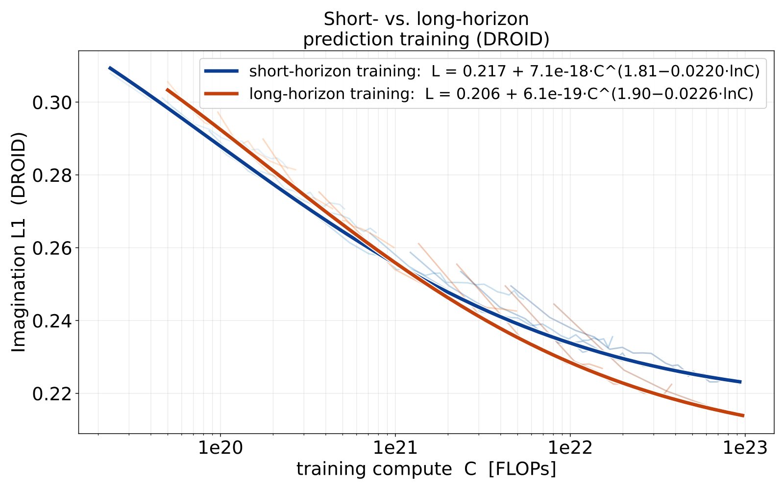
Figure 36: Short- vs. long-horizon prediction training on DROID. Out-of-distribution imagination L1 on the DROID holdout versus training compute. Faded curves are per-size checkpoints (blue: short-horizon training, orange: long-horizon training; shade encodes model size); the bold curves are the two second-order power laws fit on each recipe’s frontier. The long-horizon training law overtakes the short-horizon training one at high compute and reaches a lower irreducible floor.
图 36:DROID 上短地平与长地平预测训练。DROID 保留集分布外想象 L1 对训练算力。淡曲线为逐规模检查点(蓝:短地平训练,橙:长地平训练;深浅编码模型规模);粗曲线为各配方前沿上拟合的二阶幂律。长地平训练律在高算力处超越短地平,并达到更低的不可约底。
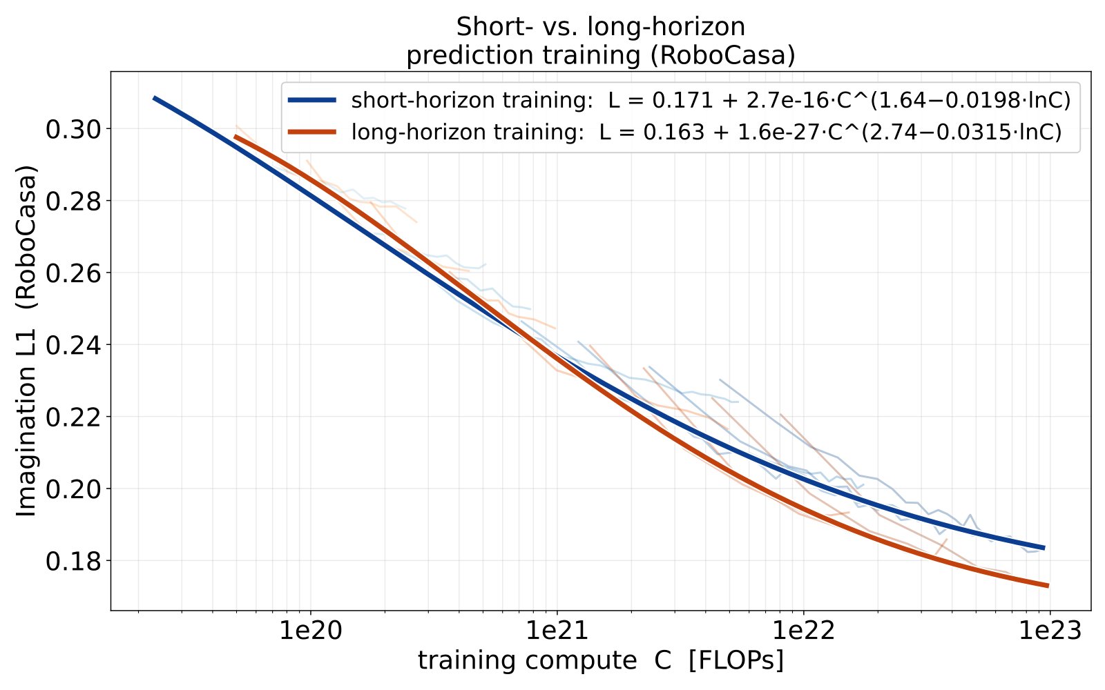
Figure 37: Short- vs. long-horizon prediction training on RoboCasa. As Figure 36, for the RoboCasa target evaluation. The same crossover and lower floor for long-horizon training hold on the simulated suite.
图 37:RoboCasa 上短地平与长地平预测训练。同图 36,针对 RoboCasa 目标评测。仿真套件上同样出现交叉与长地平训练更低的底。
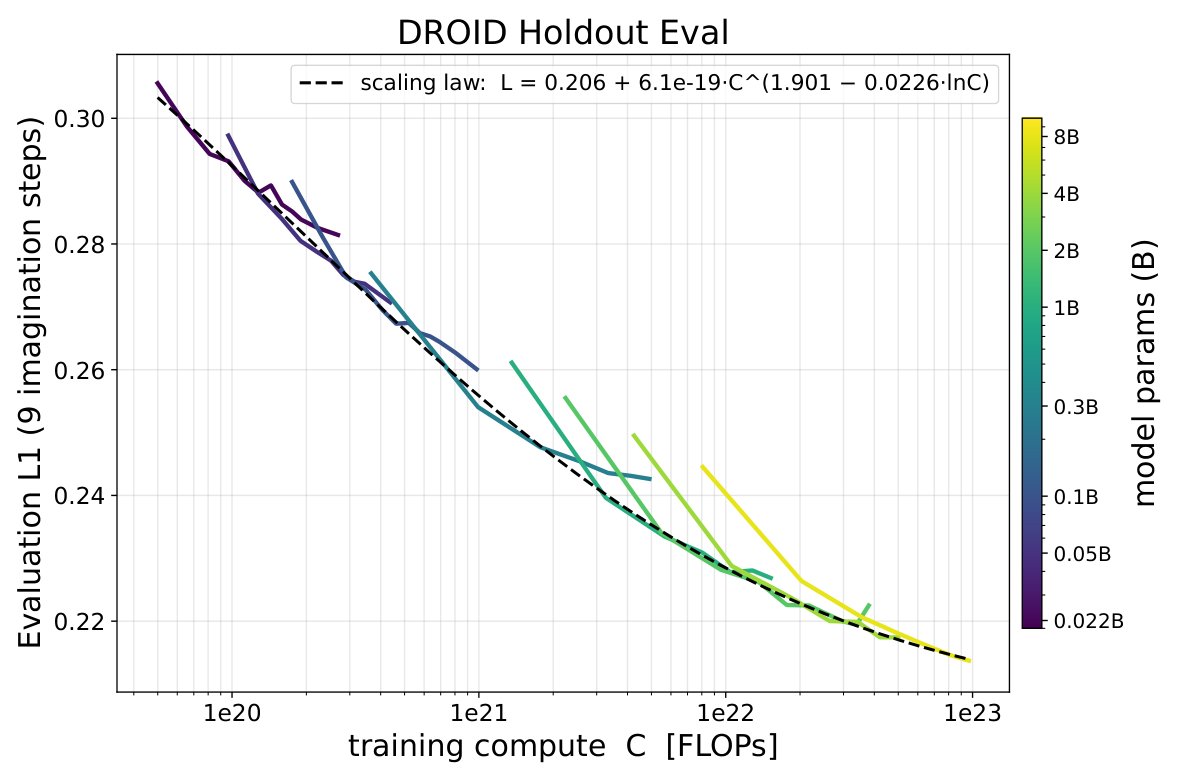
Figure 38: Long-horizon training scaling law on DROID. Long-horizon prediction training alone: per-size checkpoint curves colored by parameter count, with the fitted second-order power law (dashed) on the compute-optimal frontier of the DROID holdout evaluation.
图 38:DROID 上长地平训练缩放律。仅长地平预测训练:按参数量着色的逐规模检查点曲线,虚线为 DROID 保留评测算力最优前沿上拟合的二阶幂律。
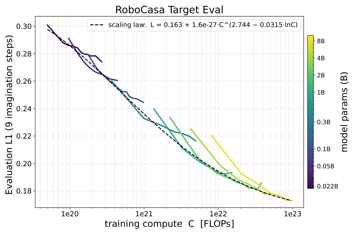
Figure 39: Long-horizon training scaling law on RoboCasa. As Figure 38, for the RoboCasa target evaluation.
图 39:RoboCasa 上长地平训练缩放律。同图 38,针对 RoboCasa 目标评测。
J.4 Per-Step Training Compute across Stages
J.4 跨阶段的逐步训练算力
Underpins the compute axis of Sections 3.1 and 3.3. The training-compute value on every scaling-law plot is accumulated as C = (per-step FLOPs) × (optimizer steps) , so the per-step computational cost of each stage sets the horizontal scale. We compute it for each run from its real configuration (view-group layout, per-cell batch size, resolution grid, view count, rollout steps, and node/GPU count), counting both the forward and backward pass. A single “per step” figure is the total the whole job performs for one optimizer update, and therefore already includes all gradient-accumulation microbatches, all data-parallel replicas, and — for rollout recipes — the autoregressive rollout unrolled over its configured steps. We report compute in PF (1 PF = 10 15 FLOPs).
支撑第 3.1 与 3.3 节的算力轴。每张缩放律图上的训练算力 按 累积,因而每阶段逐步计算代价设定横轴尺度。我们对每次运行按其真实配置(视角组布局、逐单元批量、分辨率网格、视角数、滚动步数、节点/GPU 数)计算,计入前向与反向。单一「逐步」数字是整次任务为一次优化器更新所做的总量,因此已包含全部梯度累积微批、全部数据并行副本,以及——对滚动配方——按其配置步数展开的自回归滚动。我们以 报告算力( FLOPs)。
RoboJEPA training has three stages with very different per-step computational costs. The long pretraining (flat learning-rate) phase and the short-horizon prediction training cooldown share the same cheap recipe (a short K = 2 rollout at a single 240 × 320 resolution). The long-horizon prediction training cooldown of Section 3.3 instead uses a K = 10 rollout with a KV cache and mixed 240 × 320 and 480 × 640 resolutions, and the DROID 720 × 1280 finetune (Section G.1) adds three high-resolution views on top of the KV-cached K = 10 rollout. Table 19 gives the per-step computational cost of the two cooldown/pretraining recipes at every model size, and Table 20 compares all three stages at B.
RoboJEPA 训练有三阶段,逐步计算代价差异很大。长预训练(平坦学习率)阶段与短地平预测训练冷却共享同一廉价配方(单一 分辨率上短 滚动)。第 3.3 节长地平预测训练冷却改用带 KV 缓存的 滚动并混合 与 ;DROID 微调(G.1)在 KV 缓存 滚动之上再加三路高分辨率视角。表 19 给出两种冷却/预训练配方在各模型规模的逐步计算代价,表 20 在 B 比较三阶段。
Table 19: Per-optimizer-step training compute (in PF , i.e. 10 15 FLOPs) for each model size. All values report total FLOPs per optimizer step across the full training job and are used for the compute axis of the scaling-law plots. The short-horizon training column also applies to pretraining. The short-horizon recipe is exact; the long-horizon recipe runs its rollout with a KV cache and is the estimate without the cache scaled by the measured KV-cache factor .
表 19:各模型规模每优化器步训练算力(单位 ,即 FLOPs)。全部数值报告整次训练任务每优化器步总 FLOPs,用于缩放律图的算力轴。短地平训练列亦适用于预训练。短地平配方为精确值;长地平配方用 KV 缓存跑滚动,为无缓存估计乘以测得的 KV 缓存因子 。
Table 20: Per-step training compute at B for the three stages. All values report total FLOPs per optimizer step across the full training job. One finetune step is ∼ 19 × a long-horizon training step and ∼ 62 × a short-horizon training step. The finetune uses a longer sequence: a 720 × 1280 image is a 45 × 80 = 3,600 -token grid per view (× 3 views = 10,800 tokens, versus ∼ 300 tokens/view at 240 × 320 ), and self-attention is 𝒪 (n 2) in tokens.
表 20:B 三阶段逐步训练算力。全部数值报告整次训练任务每优化器步总 FLOPs。一步微调约 长地平训练步、约 短地平训练步。微调使用更长序列: 图像每视角为 词元网格( 视角 词元,对比 每视角约 词元),而自注意力对词元数为 。
J.5 Stochastic upper-envelope selection
J.5 随机上包络选择
Extracts the compute-optimal frontier of the downstream planning success-rate (reward) curves reported in the visual abstract (Figure 1). This procedure applies to the RoboCasa downstream planning tasks, where higher success rate is better. Every model size contributes many checkpoints, so at a fixed size the (compute, success-rate) pairs are stochastic rather than a single clean curve: evaluation noise and training instabilities give a scatter of points at nearby compute values. Fitting a scaling law requires the compute-optimal upper envelope — the best achievable success rate at each compute — rather than the raw scatter, but the obvious envelope estimators are both unsatisfying. A running maximum over compute is not robust: a single lucky, high-variance checkpoint pulls the envelope up prematurely and the estimate never recovers. Fitting the law to all points instead is dragged toward the mean of the scatter, since many dominated, lower checkpoints outnumber the few near the ceiling.
提取视觉摘要(图 1)所报下游规划成功率(奖励)曲线的算力最优前沿。该程序适用于 RoboCasa 下游规划任务,成功率越高越好。每个模型规模贡献许多检查点,因而在固定规模下(算力,成功率)对是随机的而非单一干净曲线:评测噪声与训练不稳定性在邻近算力值给出点散布。拟合缩放律需要算力最优上包络——每个算力下可达成的最佳成功率——而非原始散布,但显而易见的包络估计器都不令人满意。按算力的滚动最大值不稳健:单一幸运、高方差检查点会过早抬高包络且估计永不恢复。改为对全部点拟合则会被散布均值拖拽,因许多被支配的较低检查点数量上压过少数接近天花板的点。
We instead select frontier points with a stochastic upper-envelope procedure that tracks a running estimate of the achievable ceiling and admits only points consistent with it, rejecting downward outliers before they can corrupt the running estimate. Concretely, we pool all (compute, success-rate) pairs (C i, y i) across model sizes (higher is better) and sort them by ascending compute. The running mean and variance are initialized from the first three points, which are always kept. Each subsequent point is compared against the current upper trend m − k s , where s = v and k ≥ 0 is a rejection threshold in standard-deviation units: a point is accepted onto the frontier only if it does not fall more than standard deviations below the running mean. Accepted points update and with an exponentially-weighted (West) moving-average and moving-variance update governed by a retention factor α ∈ (0, 1) , so recent frontier points dominate the running estimate while stale ones decay away; rejected points leave and untouched, so a single downward outlier can neither join the frontier nor bias the trend used to judge later points. The scaling law is then fit only on the resulting frontier set. We use α = 0.9 throughout, with a per-task rejection threshold matched to the four RoboCasa downstream planning tasks of the visual abstract: k ≈ 0.5 for the two shorter-horizon, greedy tasks, a larger k ≈ 2 for the noisier long-horizon obstacle task, and no rejection (k → ∞ , all points kept) for the object-push task, reflecting the differing success-rate evaluation noise of each task (short-horizon vs. long-horizon, and whether object interaction is involved).
我们改用随机上包络程序选择前沿点:跟踪可达成天花板的滚动估计,只接纳与之一致的点,在向下离群值腐蚀滚动估计前将其拒绝。具体地,我们汇集跨模型规模的全部(算力,成功率)对 ( 越高越好)并按算力升序排序。滚动均值 与方差 由前三点初始化,这三点始终保留。每个后续点与当前上趋势 比较,其中 , 为以标准差为单位的拒绝阈值:仅当点不低于滚动均值超过 个标准差时才接纳到前沿。被接纳的点用由保留因子 控制的指数加权(West)移动平均与移动方差更新 与 ,使近期前沿点主导滚动估计而陈旧点衰减;被拒绝的点不触碰 与 ,因而单一向下离群值既不能加入前沿,也不能偏置用于判断后续点的趋势。缩放律随后仅在所得前沿集上拟合。我们通篇用 ,并按视觉摘要四项 RoboCasa 下游规划任务匹配逐任务拒绝阈值:两个较短地平、贪心任务用 ,更噪的长地平障碍任务用更大的 ,物体推动任务不做拒绝(,保留全部点),反映各任务不同的成功率评测噪声(短地平对长地平,以及是否涉及物体交互)。
Algorithm 2 Stochastic upper-envelope (frontier) selection
算法 2:随机上包络(前沿)选择
The new-point weight (1 − α) controls how quickly the running estimate adapts: α close to retains a long memory of past frontier points and adapts slowly, while smaller α tracks recent points more aggressively. Because and are updated only on accepted points, the procedure is robust to an arbitrary number of downward outliers at any compute scale, unlike a plain running maximum. A reference implementation is provided in make_plot.py as the function stochastic_envelope.
新点权重 控制滚动估计适应速度: 接近 对过去前沿点保持长记忆、适应慢,而较小 更积极跟踪近期点。因 与 仅在被接纳点上更新,该程序对任意算力尺度上任意数量的向下离群值稳健,不同于朴素滚动最大值。参考实现以函数 stochastic_envelope 提供于 make_plot.py。
Appendix K Encoder Choice and World-Model Scaling
附录 K 编码器选择与世界模型缩放
Initially, we started the project by scaling the predictor on top of the V-JEPA 2 encoder. However, we faced numerous issues and instabilities during training. The predictor often collapsed beyond a certain model size, despite the frozen encoder, and increasing the dataset size often led to training instabilities or sometimes divergence. For both encoders, we worked with image features only. We hypothesize that this behavior can be attributed to the type of features the encoder computes.
项目最初在 V-JEPA 2 编码器之上缩放预测器。然而我们在训练中遇到诸多问题与不稳定性。尽管编码器冻结,预测器仍常在超过某规模后塌缩;增大数据集也常导致训练不稳甚至发散。对两种编码器我们都只使用图像特征。我们假设该行为可归因于编码器计算的特征类型。
Table 21 restates published evaluations of V-JEPA 2 (Assran et al., 2025) and V-JEPA 2.1 (Mur-Labadia et al., 2026) on the classification, semantic segmentation, and depth estimation benchmarks shown in Figure 2 of the latter paper, together with IntPhys2 (Bordes et al., 2025) results reported by Punzo et al. (2026). These are results from the cited papers, not evaluations conducted in this work.
表 21 重述 V-JEPA 2(Assran 等,2025)与 V-JEPA 2.1(Mur-Labadia 等,2026)在后一文图 2 所示分类、语义分割与深度估计基准上的已发表评测,以及 Punzo 等(2026)报告的 IntPhys2(Bordes 等,2025)结果。这些是被引论文的结果,非本工作自行评测。
Table 21 shows that the V-JEPA 2 and V-JEPA 2.1 encoders perform on par on image and video understanding tasks, measured through image and video classification, and V-JEPA 2.1 even obtains a lower reported score on the IntPhys2 intuitive physics task than V-JEPA 2. On the other hand, V-JEPA 2.1 substantially outperforms V-JEPA 2 on dense tasks such as depth estimation and semantic segmentation. Given this large gap, we hypothesize that high-quality dense features are the most important features for scaling robotic world models, even more important than features associated with physical understanding.
表 21 显示,以图像与视频分类度量,V-JEPA 2 与 V-JEPA 2.1 编码器在图像与视频理解任务上表现相当,且 V-JEPA 2.1 在 IntPhys2 直观物理任务上报告分数甚至低于 V-JEPA 2。另一方面,V-JEPA 2.1 在深度估计与语义分割等稠密任务上大幅超过 V-JEPA 2。鉴于该差距,我们假设高质量稠密特征是缩放机器人世界模型最重要的特征,甚至比与物理理解相关的特征更重要。
Table 21: Restated results from Mur-Labadia et al. (2026) (Tables 8–9) and Punzo et al. (2026) (Table 1, IntPhys2); V-JEPA 2 classification results are also reported by Assran et al. (2025) (Table 4). We distinguish global tasks (action recognition, image classification, and intuitive physics) from dense tasks (semantic segmentation and depth estimation), following the grouping in Figure 2 of Mur-Labadia et al. (2026). Classification uses attentive probes; segmentation and depth use linear probes, with frozen encoders. IntPhys2 reports mean violation-of-expectation (VOE) accuracy over three seeds with a temporal attentive probe at each model’s best reported layer. Higher accuracy and mIoU, and lower RMSE, are better. Model sizes and pretraining recipes differ, so this is not a controlled ablation.
表 21:重述自 Mur-Labadia 等(2026)(表 8–9)与 Punzo 等(2026)(表 1,IntPhys2);V-JEPA 2 分类结果亦由 Assran 等(2025)(表 4)报告。我们按 Mur-Labadia 等(2026)图 2 的分组,区分全局任务(动作识别、图像分类、直观物理)与稠密任务(语义分割、深度估计)。分类用注意力探针;分割与深度用线性探针,编码器冻结。IntPhys2 报告三随机种子上平均违背期望(VOE)准确率,在各模型报告最佳层用时间注意力探针。准确率与 mIoU 越高、RMSE 越低越好。模型规模与预训练配方不同,因而这不是受控消融。