Exploration by Random Network Distillation

用随机网络蒸馏做探索

Yuri BurdaOpenAIHarrison EdwardsOpenAIAmos StorkeyUniv. of EdinburghOleg KlimovOpenAI Thanks:  Alphabetical ordering; the first two authors contributed equally.

Abstract

摘要

We introduce an exploration bonus for deep reinforcement learning methods that is easy to implement and adds minimal overhead to the computation performed. The bonus is the error of a neural network predicting features of the observations given by a fixed randomly initialized neural network. We also introduce a method to flexibly combine intrinsic and extrinsic rewards. We find that the random network distillation (RND) bonus combined with this increased flexibility enables significant progress on several hard exploration Atari games. In particular we establish state of the art performance on Montezuma’s Revenge, a game famously difficult for deep reinforcement learning methods. To the best of our knowledge, this is the first method that achieves better than average human performance on this game without using demonstrations or having access to the underlying state of the game, and occasionally completes the first level.

我们为深度强化学习方法引入一种探索奖励：实现简单，对计算几乎不增加额外负担。该奖励是一个神经网络在预测由固定随机初始化神经网络给出的观测特征时的误差。我们还引入一种灵活组合内在奖励与外在奖励的方法。我们发现，随机网络蒸馏（RND）奖励加上这种更大的灵活性，能在若干难探索 Atari 游戏上取得显著进展。尤其是，我们在以难著称的 Montezuma’s Revenge 上达到当时最优表现。据我们所知，这是首个在不使用示范、也不访问游戏底层状态的前提下，在该游戏上超过普通人类平均水平、并偶尔通关第一关的方法。

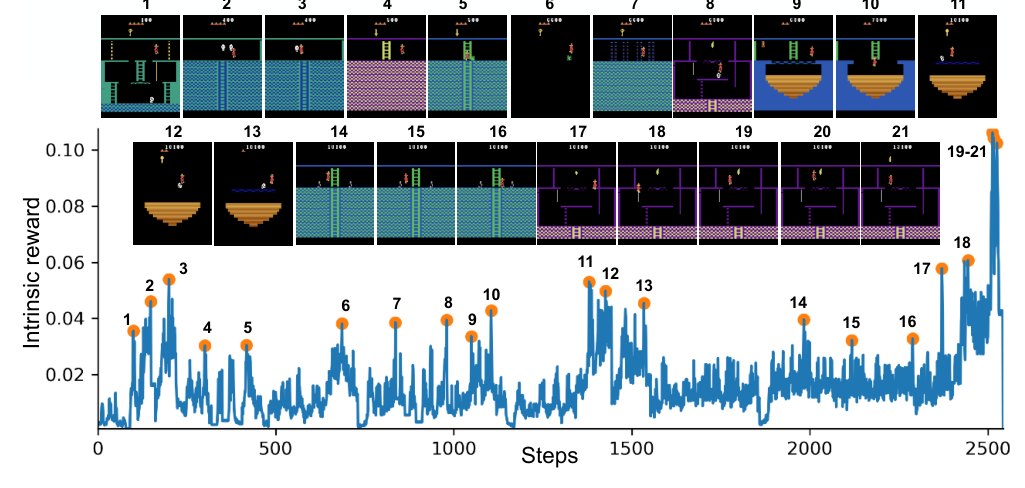
Figure 1: RND exploration bonus over the course of the first episode where the agent picks up the torch (19-21). To do so the agent passes 17 rooms and collects gems, keys, a sword, an amulet, and opens two doors. Many of the spikes in the exploration bonus correspond to meaningful events: losing a life (2,8,10,21), narrowly escaping an enemy (3,5,6,11,12,13,14,15), passing a difficult obstacle (7,9,18), or picking up an object (20,21). The large spike at the end corresponds to a novel experience of interacting with the torch, while the smaller spikes correspond to relatively rare events that the agent has nevertheless experienced multiple times. See here for videos.

图 1：智能体首次捡起火把（19–21）的那一局里，RND 探索奖励随时间的变化。为此智能体穿过 17 个房间，收集宝石、钥匙、剑、护身符，并打开两扇门。探索奖励上的许多尖峰对应有意义的事件：失去一条命（2,8,10,21）、险些躲开敌人（3,5,6,11,12,13,14,15）、通过困难障碍（7,9,18）、或捡起物品（20,21）。末尾的大尖峰对应与火把交互这一新颖体验，较小尖峰对应相对罕见但智能体已多次经历的事件。视频见文中链接。

1 Introduction

1 引言

Reinforcement learning (RL) methods work by maximizing the expected return of a policy. This works well when the environment has dense rewards that are easy to find by taking random sequences of actions, but tends to fail when the rewards are sparse and hard to find. In reality it is often impractical to engineer dense reward functions for every task one wants an RL agent to solve. In these situations methods that explore the environment in a directed way are necessary.

强化学习（RL）方法通过最大化策略的期望回报工作。当环境奖励稠密、靠随机动作序列就容易碰到时，这很有效；当奖励稀疏且难找时，往往失败。现实中，很难为每个想让 RL 智能体解决的任务都手工设计稠密奖励函数。此时需要能有方向地探索环境的方法。

Recent developments in RL seem to suggest that solving the most challenging tasks (Silver et al. 2016; Zoph & Le 2016; Horgan et al. 2018; Espeholt et al. 2018; OpenAI 2018; OpenAI et al. 2018) requires processing large numbers of samples obtained from running many copies of the environment in parallel. In light of this it is desirable to have exploration methods that scale well with large amounts of experience. However many of the recently introduced exploration methods based on counts, pseudo-counts, information gain or prediction gain are difficult to scale up to large numbers of parallel environments.

RL 的近期发展似乎表明：解决最具挑战性的任务（Silver et al. 2016；Zoph & Le 2016；Horgan et al. 2018；Espeholt et al. 2018；OpenAI 2018；OpenAI et al. 2018）需要处理从大量并行环境副本中获得的海量样本。因此，希望探索方法能随大量经验良好扩展。然而，许多近期基于计数、伪计数、信息增益或预测增益的探索方法，很难扩展到大量并行环境。

This paper introduces an exploration bonus that is particularly simple to implement, works well with high-dimensional observations, can be used with any policy optimization algorithm, and is efficient to compute as it requires only a single forward pass of a neural network on a batch of experience. Our exploration bonus is based on the observation that neural networks tend to have significantly lower prediction errors on examples similar to those on which they have been trained. This motivates the use of prediction errors of networks trained on the agent’s past experience to quantify the novelty of new experience.

本文引入一种探索奖励：实现特别简单，适合高维观测，可与任意策略优化算法合用，计算高效——只需对一批经验做一次神经网络前向。我们的探索奖励基于如下观察：神经网络在与训练样本相似的例子上，预测误差往往显著更低。这促使我们用在智能体过往经验上训练的网络的预测误差，来量化新经验的新颖性。

As pointed out by many authors, agents that maximize such prediction errors tend to get attracted to transitions where the answer to the prediction problem is a stochastic function of the inputs. For example if the prediction problem is that of predicting the next observation given the current observation and agent’s action (forward dynamics), an agent trying to maximize this prediction error will tend to seek out stochastic transitions, like those involving randomly changing static noise on a TV, or outcomes of random events such as coin tosses. This observation motivated the use of methods that quantify the relative improvement of the prediction, rather than its absolute error. Unfortunately, as previously mentioned, such methods are hard to implement efficiently.

许多作者指出：最大化这类预测误差的智能体，往往会被吸引到「预测问题的答案是输入的随机函数」的转移上。例如，若预测问题是根据当前观测与动作预测下一观测（前向动力学），则最大化该预测误差的智能体往往寻求随机转移，如电视上随机变化的静态噪声，或抛硬币一类随机事件的结果。这一观察促使人们改用量化预测相对改进、而非绝对误差的方法。但如前所述，这类方法很难高效实现。

We propose an alternative solution to this undesirable stochasticity by defining an exploration bonus using a prediction problem where the answer is a deterministic function of its inputs. Namely we predict the output of a fixed randomly initialized neural network on the current observation.

我们提出另一种解决这种不良随机性的方案：用一个预测问题定义探索奖励，使其答案是输入的确定性函数。具体而言，我们预测一个固定随机初始化神经网络在当前观测上的输出。

Atari games have been a standard benchmark for deep reinforcement learning algorithms since the pioneering work by Mnih et al. 2013. Bellemare et al. 2016 identified among these games the hard exploration games with sparse rewards: Freeway, Gravitar, Montezuma’s Revenge, Pitfall!, Private Eye, Solaris, and Venture. RL algorithms tend to struggle on these games, often not finding even a single positive reward.

自 Mnih et al. 2013 的开创工作以来，Atari 游戏一直是深度强化学习算法的标准基准。Bellemare et al. 2016 在这些游戏中识别出稀疏奖励的难探索游戏：Freeway、Gravitar、Montezuma’s Revenge、Pitfall!、Private Eye、Solaris 与 Venture。RL 算法往往在这些游戏上挣扎，甚至经常找不到哪怕一次正奖励。

In particular, Montezuma’s Revenge is considered to be a difficult problem for RL agents, requiring a combination of mastery of multiple in-game skills to avoid deadly obstacles, and finding rewards that are hundreds of steps apart from each other even under optimal play. Significant progress has been achieved by methods with access to either expert demonstrations (Pohlen et al. 2018; Aytar et al. 2018; Garmulewicz et al. 2018), special access to the underlying emulator state (Tang et al. 2017; Stanton & Clune 2018), or both (Salimans & Chen 2018). However without such aids, progress on the exploration problem in Montezuma’s Revenge has been slow, with the best methods finding about half the rooms (Bellemare et al. 2016). For these reasons we provide extensive ablations of our method on this environment.

尤其是，Montezuma’s Revenge 被认为对 RL 智能体很难：既要掌握多种游戏内技能以避开致命障碍，又要找到即便最优游玩也相隔数百步的奖励。已有方法通过专家示范（Pohlen et al. 2018；Aytar et al. 2018；Garmulewicz et al. 2018）、特殊访问模拟器底层状态（Tang et al. 2017；Stanton & Clune 2018），或二者兼有（Salimans & Chen 2018）取得显著进展。但没有这些辅助时，Montezuma’s Revenge 上的探索进展缓慢，最好的方法大约只找到一半房间（Bellemare et al. 2016）。因此我们在该环境上对本方法做了大量消融。

We find that even when disregarding the extrinsic reward altogether, an agent maximizing the RND exploration bonus consistently finds more than half of the rooms in Montezuma’s Revenge. To combine the exploration bonus with the extrinsic rewards we introduce a modification of Proximal Policy Optimization (PPO, Schulman et al. 2017) that uses two value heads for the two reward streams. This allows the use of different discount rates for the different rewards, and combining episodic and non-episodic returns. With this additional flexibility, our best agent often finds 22 out of the 24 rooms on the first level in Montezuma’s Revenge, and occasionally (though not frequently) passes the first level. The same method gets state of the art performance on Venture and Gravitar.

我们发现：即便完全忽略外在奖励，最大化 RND 探索奖励的智能体也能稳定地找到 Montezuma’s Revenge 一半以上的房间。为把探索奖励与外在奖励结合，我们对近端策略优化（PPO，Schulman et al. 2017）做了修改，为两路奖励流使用两个价值头。这允许对不同奖励使用不同折扣率，并组合回合制与非回合制回报。有了这种额外灵活性，我们最好的智能体常能在 Montezuma’s Revenge 第一关找到 24 个房间中的 22 个，并偶尔（虽不频繁）通过第一关。同一方法在 Venture 与 Gravitar 上达到当时最优。

2 Method

2 方法

2.1 Exploration bonuses

2.1 探索奖励

Exploration bonuses are a class of methods that encourage an agent to explore even when the environment’s reward $e_{t}$ is sparse. They do so by replacing $e_{t}$ with a new reward $r_{t}=e_{t}+i_{t}$, where $i_{t}$ is the exploration bonus associated with the transition at time $t$.

探索奖励是一类方法：即便环境奖励 $e_{t}$ 稀疏，也鼓励智能体探索。做法是把 $e_{t}$ 替换为新奖励 $r_{t}=e_{t}+i_{t}$，其中 $i_{t}$ 是时刻 $t$ 转移关联的探索奖励。

To encourage the agent to visit novel states, it is desirable for $i_{t}$ to be higher in novel states than in frequently visited ones. Count-based exploration methods provide an example of such bonuses. In a tabular setting with a finite number of states one can define $i_{t}$ to be a decreasing function of the visitation count $n_{t}({\bm{s}})$ of the state ${\bm{s}}$. In particular $i_{t}=1/n_{t}({\bm{s}})$ and $i_{t}=1/\sqrt{n_{t}({\bm{s}})}$ have been used in prior work (Bellemare et al. 2016; Ostrovski et al. 2018). In non-tabular cases it is not straightforward to produce counts, as most states will be visited at most once. One possible generalization of counts to non-tabular settings is pseudo-counts (Bellemare et al. 2016) which uses changes in state density estimates as an exploration bonus. In this way the counts derived from the density model can be positive even for states that have not been visited in the past, provided they are similar to previously visited states.

为鼓励智能体访问新颖状态，希望 $i_{t}$ 在新颖状态高于频繁访问状态。基于计数的探索方法提供了这类奖励的例子。在状态有限的表格设定中，可把 $i_{t}$ 定义为访问计数 $n_{t}({\bm{s}})$ 的递减函数。先前工作使用过 $i_{t}=1/n_{t}({\bm{s}})$ 与 $i_{t}=1/\sqrt{n_{t}({\bm{s}})}$（Bellemare et al. 2016；Ostrovski et al. 2018）。在非表格情形下产生计数并不直接，因为多数状态最多访问一次。一种把计数推广到非表格设定的做法是伪计数（Bellemare et al. 2016），用状态密度估计的变化作为探索奖励。这样，即便过去未访问过的状态，只要与已访问状态相似，导出的计数也可为正。

An alternative is to define $i_{t}$ as the prediction error for a problem related to the agent’s transitions. Generic examples of such problems include forward dynamics (Schmidhuber 1991b; Stadie et al. 2015; Achiam & Sastry 2017; Pathak et al. 2017; Burda et al. 2018) and inverse dynamics (Haber et al. 2018). Non-generic prediction problems can also be used if specialized information about the environment is available, like predicting physical properties of objects the agent interacts with (Denil et al. 2016). Such prediction errors tend to decrease as the agent collects more experience similar to the current one. For this reason even trivial prediction problems like predicting a constant zero function can work as exploration bonuses (Fox et al. 2018).

另一种做法是把 $i_{t}$ 定义为与智能体转移相关的某个问题的预测误差。通用例子包括前向动力学（Schmidhuber 1991b；Stadie et al. 2015；Achiam & Sastry 2017；Pathak et al. 2017；Burda et al. 2018）与逆动力学（Haber et al. 2018）。若有环境的专用信息，也可用非通用预测问题，如预测智能体交互物体的物理属性（Denil et al. 2016）。这类预测误差往往随智能体收集到更多与当前相似的经验而下降。因此，即便像预测常数零函数这样的平凡预测问题，也可作为探索奖励（Fox et al. 2018）。

2.2 Random Network Distillation

2.2 随机网络蒸馏

This paper introduces a different approach where the prediction problem is randomly generated. This involves two neural networks: a fixed and randomly initialized target network which sets the prediction problem, and a predictor network trained on data collected by the agent. The target network takes an observation to an embedding $f:\mathcal{O}\to\mathbb{R}^{k}$ and the predictor neural network $\hat{f}:\mathcal{O}\to\mathbb{R}^{k}$ is trained by gradient descent to minimize the expected MSE $\|\hat{f}({\textnormal{x}};\theta)-f({\textnormal{x}})\|^{2}$ with respect to its parameters $\theta_{\hat{f}}$. This process distills a randomly initialized neural network into a trained one. The prediction error is expected to be higher for novel states dissimilar to the ones the predictor has been trained on.

本文引入另一种方法：预测问题随机生成。它涉及两个神经网络：固定且随机初始化的 目标 网络，用于设定预测问题；以及在智能体收集的数据上训练的 预测 网络。目标网络把观测映射到嵌入 $f:\mathcal{O}\to\mathbb{R}^{k}$，预测网络 $\hat{f}:\mathcal{O}\to\mathbb{R}^{k}$ 用梯度下降最小化期望 MSE $\|\hat{f}({\textnormal{x}};\theta)-f({\textnormal{x}})\|^{2}$（对其参数 $\theta_{\hat{f}}$）。该过程把随机初始化网络蒸馏进训练好的网络。对与预测器训练样本不相似的新颖状态，预测误差预期更高。

To build intuition we consider a toy model of this process on MNIST. We train a predictor neural network to mimic a randomly initialized target network on training data consisting of a mixture of images with the label 0 and of a target class, varying the proportion of the classes, but not the total number of training examples. We then test the predictor network on the unseen test examples of the target class and report the MSE. In this model the zeros are playing the role of states that have been seen many times before, and the target class is playing the role of states that have been visited infrequently. The results are shown in Figure 3. The figure shows that test error decreases as a function of the number of training examples in the target class, suggesting that this method can be used to detect novelty. Figure 1 shows that the intrinsic reward is high in novel states in an episode of Montezuma’s Revenge.

为建立直觉，我们在 MNIST 上考虑该过程的玩具模型。训练预测网络去模仿随机初始化的目标网络，训练数据由标签为 0 的图像与某一目标类图像混合而成，改变两类比例但保持训练样本总数不变。然后在未见过的目标类测试样本上测试预测网络并报告 MSE。此模型中，零扮演「已多次见过的状态」，目标类扮演「访问较少的状态」。结果见图 3：测试误差随目标类训练样本数减少，说明该方法可用于检测新颖性。图 1 显示在 Montezuma’s Revenge 的一局里，内在奖励在新颖状态上更高。

One objection to this method is that a sufficiently powerful optimization algorithm might find a predictor that mimics the target random network perfectly on any input (for example the target network itself would be such a predictor). However the above experiment on MNIST shows that standard gradient-based methods don’t overgeneralize in this undesirable way.

对该方法的一种质疑是：足够强大的优化算法或许能找到在任意输入上都完美模仿目标随机网络的预测器（例如目标网络本身）。但上述 MNIST 实验表明，标准基于梯度的方法不会以这种不良方式过度泛化。

2.2.1 Sources of prediction errors

In general, prediction errors can be attributed to a number of factors:

2.2.1 预测误差的来源

一般而言，预测误差可归因于若干因素：

1. Amount of training data. Prediction error is high where few similar examples were seen by the predictor (epistemic uncertainty).

1. 训练数据量。在预测器见过的相似例子很少处，预测误差高（认知不确定性）。

2. Stochasticity. Prediction error is high because the target function is stochastic (aleatoric uncertainty). Stochastic transitions are a source of such error for forward dynamics prediction.

2. 随机性。因目标函数随机，预测误差高（偶然不确定性）。对前向动力学预测，随机转移是此类误差的来源。

3. Model misspecification. Prediction error is high because necessary information is missing, or the model class is too limited to fit the complexity of the target function.

3. 模型设定错误。因缺少必要信息，或模型类过窄无法拟合目标函数复杂度，预测误差高。

4. Learning dynamics. Prediction error is high because the optimization process fails to find a predictor in the model class that best approximates the target function.

4. 学习动态。因优化过程未能在模型类中找到最逼近目标函数的预测器，预测误差高。

Factor 1 is what allows one to use prediction error as an exploration bonus. In practice the prediction error is caused by a combination of all of these factors, not all of them desirable.

因素 1 使人们能把预测误差用作探索奖励。实践中预测误差由所有这些因素共同造成，并非全部合意。

For instance if the prediction problem is forward dynamics, then factor 2 results in the ‘noisy-TV’ problem. This is the thought experiment where an agent that is rewarded for errors in the prediction of its forward dynamics model gets attracted to local sources of entropy in the environment. A TV showing white noise would be such an attractor, as would a coin flip.

例如，若预测问题是前向动力学，则因素 2 导致「嘈杂电视」问题：若智能体因前向动力学模型的预测误差而获奖励，就会被环境中的局部熵源吸引。播放白噪声的电视会是这样的吸引子，抛硬币亦然。

To avoid the undesirable factors 2 and 3, methods such as those by Schmidhuber 1991a; Oudeyer et al. 2007; Lopes et al. 2012; Achiam & Sastry 2017 instead use a measurement of how much the prediction model improves upon seeing a new datapoint. However these approaches tend to be computationally expensive and hence difficult to scale.

为避免不良因素 2 与 3，Schmidhuber 1991a；Oudeyer et al. 2007；Lopes et al. 2012；Achiam & Sastry 2017 等方法改用「见到新数据点后预测模型改进多少」的度量。但这些方法往往计算昂贵，因而难扩展。

RND obviates factors 2 and 3 since the target network can be chosen to be deterministic and inside the model-class of the predictor network.

RND 消解了因素 2 与 3，因为目标网络可选为确定性的，并落在预测网络的模型类内。

2.2.2 Relation to uncertainty quantification

RND prediction error is related to an uncertainty quantification method introduced by Osband et al. 2018. Namely, consider a regression problem with data distribution $D=\{x_{i},y_{i}\}_{i}$. In the Bayesian setting we would consider a prior $p(\theta^{*})$ over the parameters of a mapping $f_{\theta^{*}}$ and calculate the posterior after updating on the evidence.

2.2.2 与不确定性量化的关系

RND 预测误差与 Osband et al. 2018 引入的一种不确定性量化方法相关。考虑数据分布为 $D=\{x_{i},y_{i}\}_{i}$ 的回归问题。在贝叶斯设定下，我们会对映射 $f_{\theta^{*}}$ 的参数考虑先验 $p(\theta^{*})$，并在证据更新后计算后验。

Let $\mathcal{F}$ be the distribution over functions $g_{\theta}=f_{\theta}+f_{\theta^{*}}$, where $\theta^{*}$ is drawn from $p(\theta^{*})$ and $\theta$ is given by minimizing the expected prediction error

设 $\mathcal{F}$ 为函数 $g_{\theta}=f_{\theta}+f_{\theta^{*}}$ 上的分布，其中 $\theta^{*}$ 从 $p(\theta^{*})$ 抽取，$\theta$ 由最小化期望预测误差得到

$$\theta=\argmin_{\theta}\mathbb{E}_{(x_{i},y_{i})\sim D}\|f_{\theta}(x_{i})+f_{\theta^{*}}(x_{i})-y_{i}\|^{2}+\mathcal{R}(\theta), \tag{1}$$

where $\mathcal{R}(\theta)$ is a regularization term coming from the prior (see Lemma 3, Osband et al. 2018). Osband et al. 2018 argue (by analogy to the case of Bayesian linear regression) that the ensemble $\mathcal{F}$ is an approximation of the posterior.

其中 $\mathcal{R}(\theta)$ 是来自先验的正则项（见 Lemma 3，Osband et al. 2018）。Osband et al. 2018 论证（类比贝叶斯线性回归情形）集成 $\mathcal{F}$ 是后验的近似。

If we specialize the regression targets $y_{i}$ to be zero, then the optimization problem $\argmin_{\theta}\mathbb{E}_{(x_{i},y_{i})\sim D}\|f_{\theta}(x_{i})+f_{\theta^{*}}(x_{i})\|^{2}$ is equivalent to distilling a randomly drawn function from the prior. Seen from this perspective, each coordinate of the output of the predictor and target networks would correspond to a member of an ensemble (with parameter sharing amongst the ensemble), and the MSE would be an estimate of the predictive variance of the ensemble (assuming the ensemble is unbiased). In other words the distillation error could be seen as a quantification of uncertainty in predicting the constant zero function.

若把回归目标 $y_{i}$ 特化为零，则优化问题 $\argmin_{\theta}\mathbb{E}_{(x_{i},y_{i})\sim D}\|f_{\theta}(x_{i})+f_{\theta^{*}}(x_{i})\|^{2}$ 等价于蒸馏一个从先验中随机抽取的函数。由此视角，预测器与目标网络输出的每个坐标对应集成中的一个成员（成员间参数共享），MSE 是该集成预测方差的估计（假定集成无偏）。换言之，蒸馏误差可视为在预测常数零函数时的不确定性量化。

2.3 Combining intrinsic and extrinsic returns

2.3 组合内在与外在回报

In preliminary experiments that used only intrinsic rewards, treating the problem as non-episodic resulted in better exploration. In that setting the return is not truncated at “game over”. We argue that this is a natural way to do exploration in simulated environments, since the agent’s intrinsic return should be related to all the novel states that it could find in the future, regardless of whether they all occur in one episode or are spread over several. It is also argued in (Burda et al. 2018) that using episodic intrinsic rewards can leak information about the task to the agent.

在仅使用内在奖励的初步实验中，把问题当作非回合制处理带来更好的探索。该设定下回报不在「game over」处截断。我们认为这是在模拟环境中做探索的自然方式：智能体的内在回报应与它未来能找到的所有新颖状态相关，无论它们集中在一局还是分散在多局。Burda et al. 2018 也论证：使用回合制内在奖励可能向智能体泄漏任务信息。

We also argue that this is closer to how humans explore games. For example let’s say Alice is playing a videogame and is attempting a tricky maneuver to reach a suspected secret room. Because the maneuver is tricky the chance of a game over is high, but the payoff to Alice’s curiosity will be high if she succeeds. If Alice is modelled as an episodic reinforcement learning agent, then her future return will be exactly zero if she gets a game over, which might make her overly risk averse. The real cost of a game over to Alice is the opportunity cost incurred by having to play through the game from the beginning (which is presumably less interesting to Alice having played the game for some time).

我们还认为这更接近人类探索游戏的方式。例如，Alice 在玩电子游戏，尝试一个刁钻操作以进入疑似秘密房间。操作刁钻，game over 概率高，但若成功，对 Alice 好奇心的回报也高。若把 Alice 建模为回合制强化学习智能体，一旦 game over，她的未来回报恰好为零，可能使她过于规避风险。对 Alice 来说，game over 的真实代价是必须从开头重玩所带来的机会成本（玩过一段时间后，开头通常更无趣）。

However using non-episodic returns for extrinsic rewards could be exploited by a strategy that finds a reward close to the beginning of the game, deliberately restarts the game by getting a game over, and repeats this in an endless cycle.

然而，对外在奖励使用非回合制回报，可能被一种策略利用：在游戏开头附近找到奖励，故意通过 game over 重启，再无限循环。

It is not obvious how to estimate the combined value of the non-episodic stream of intrinsic rewards $i_{t}$ and the episodic stream of extrinsic rewards $e_{t}$. Our solution is to observe that the return is linear in the rewards and so can be decomposed as a sum $R=R_{E}+R_{I}$ of the extrinsic and intrinsic returns respectively. Hence we can fit two value heads $V_{E}$ and $V_{I}$ separately using their respective returns, and combine them to give the value function $V=V_{E}+V_{I}$. This same idea can also be used to combine reward streams with different discount factors.

如何估计非回合制内在奖励流 $i_{t}$ 与回合制外在奖励流 $e_{t}$ 的组合价值并不显然。我们的方案是：注意到回报对奖励线性，因而可分解为外在与内在回报之和 $R=R_{E}+R_{I}$。因此可用各自回报分别拟合两个价值头 $V_{E}$ 与 $V_{I}$，再组合得到价值函数 $V=V_{E}+V_{I}$。同一想法也可用于组合具有不同折扣因子的奖励流。

Note that even where one is not trying to combine episodic and non-episodic reward streams, or reward streams with different discount factors, there may still be a benefit to having separate value functions since there is an additional supervisory signal to the value function. This may be especially important for exploration bonuses since the extrinsic reward function is stationary whereas the intrinsic reward function is non-stationary.

注意：即便不试图组合回合制与非回合制奖励流，或不组合不同折扣因子的奖励流，使用分离的价值函数仍可能有益，因为价值函数多了一路监督信号。这对探索奖励尤其重要，因为外在奖励函数平稳，而内在奖励函数非平稳。

2.4 Reward and Observation Normalization

2.4 奖励与观测归一化

One issue with using prediction error as an exploration bonus is that the scale of the reward can vary greatly between different environments and at different points in time, making it difficult to choose hyperparameters that work in all settings. In order to keep the rewards on a consistent scale we normalized the intrinsic reward by dividing it by a running estimate of the standard deviations of the intrinsic returns.

用预测误差作探索奖励的一个问题是：奖励尺度在不同环境、不同时刻可能差异很大，难以选择在所有设定都管用的超参数。为使奖励保持一致尺度，我们用内在回报标准差的运行估计去除以内在奖励。

Observation normalization is often important in deep learning but it is crucial when using a random neural network as a target, since the parameters are frozen and hence cannot adjust to the scale of different datasets. Lack of normalization can result in the variance of the embedding being extremely low and carrying little information about the inputs. To address this issue we use an observation normalization scheme often used in continuous control problems whereby we whiten each dimension by subtracting the running mean and then dividing by the running standard deviation. We then clip the normalized observations to be between -5 and 5. We initialize the normalization parameters by stepping a random agent in the environment for a small number of steps before beginning optimization. We use the same observation normalization for both predictor and target networks but not the policy network.

观测归一化在深度学习中往往重要，但在以随机神经网络为目标时尤为关键：参数被冻结，无法适配不同数据集的尺度。缺乏归一化会导致嵌入方差极低，几乎不携带输入信息。为此我们采用连续控制中常用的观测归一化方案：对各维减去运行均值再除以运行标准差，并将归一化观测裁剪到 -5 与 5 之间。优化开始前，先让随机智能体在环境中走少量步以初始化归一化参数。预测器与目标网络使用相同观测归一化，策略网络不用。

3 Experiments

3 实验

We begin with an intrinsic reward only experiment on Montezuma’s Revenge in Section 3.1 to isolate the inductive bias of the RND bonus, follow by extensive ablations of RND on Montezuma’s Revenge in Sections 3.2-3.4 to understand the factors that contribute to RND’s performance, and conclude with a comparison to baseline methods on 6 hard exploration Atari games in Section 3.6. For details of hyperparameters and architectures we refer the reader to Appendices A.3 and A.4. Most experiments are run for 30K rollouts of length $128$ per environment with $128$ parallel environments, for a total of $1.97$ billion frames of experience.

我们先在 3.1 节对 Montezuma’s Revenge 做仅内在奖励实验，以隔离 RND 奖励的归纳偏置；再在 3.2–3.4 节对 Montezuma’s Revenge 做大量消融，以理解贡献 RND 表现的因素；最后在 3.6 节与基线方法在 6 个难探索 Atari 游戏上比较。超参数与架构细节见附录 A.3 与 A.4。多数实验运行 30K 次 rollout，每次长度 $128$，并行 128 个环境，共 $1.97$ billion 帧经验。

3.1 Pure exploration

3.1 纯探索

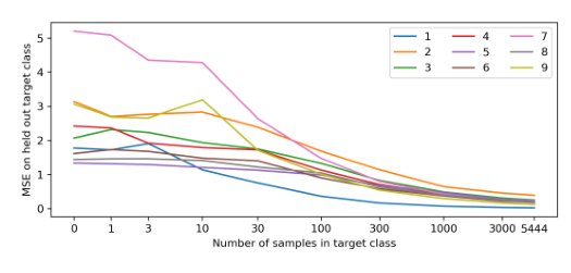
Figure 2: Novelty detection on MNIST: a predictor network mimics a randomly initialized target network. The training data consists of varying proportions of images from class “0” and a target class. Each curve shows the test MSE on held out target class examples plotted against the number of training examples of the target class (log scale).

图 2：MNIST 上的新颖性检测：预测网络模仿随机初始化的目标网络。训练数据由类「0」与某一目标类图像按不同比例组成。每条曲线给出在留出目标类样本上的测试 MSE，对目标类训练样本数（对数刻度）作图。

In this section we explore the performance of RND in the absence of any extrinsic reward. In Section 2.3 we argued that exploration with RND might be more natural in the non-episodic setting. By comparing the performance of the pure exploration agent in episodic and non-episodic settings we can see if this observation translates to improved exploration performance.

本节考察在没有任何外在奖励时 RND 的表现。2.3 节论证：用 RND 探索在非回合制设定下可能更自然。通过比较纯探索智能体在回合制与非回合制设定下的表现，可看该观察是否转化为更好的探索表现。

We report two measures of exploration performance in Figure 3: mean episodic return, and the number of rooms the agent finds over the training run. Since the pure exploration agent is not aware of the extrinsic rewards or number of rooms, it is not directly optimizing for any of these measures. However obtaining some rewards in Montezuma’s Revenge (like getting the key to open a door) is required for accessing more interesting states in new rooms, and hence we observe the extrinsic reward increasing over time up to some point. The best return is achieved when the agent interacts with some of the objects, but the agent has no incentive to keep doing the same once such interactions become repetitive, hence returns are not consistently high.

我们在图 3 中报告两项探索表现度量：平均回合回报，以及训练过程中智能体找到的房间数。由于纯探索智能体不知外在奖励或房间数，它并不直接优化这些度量。但在 Montezuma’s Revenge 中获得某些奖励（如拿钥匙开门）是进入新房间中更有趣状态所必需的，因此我们观察到外在奖励会随时间上升到某一点。最佳回报出现在智能体与某些物体交互时，但一旦此类交互变得重复，智能体没有动力继续，故回报并非一直很高。

We clearly see in Figure 3 that on both measures of exploration the non-episodic agent performs best, consistent with the discussion in Section 2.3. The non-episodic setting with $\gamma_{I}=0.999$ explores more rooms than $\gamma_{I}=0.99$, with one of the runs exploring 21 rooms. The best return achieved by 4 out 5 runs of this setting was 6,700.

从图 3 可清楚看到：在两项探索度量上非回合制智能体表现最好，与 2.3 节讨论一致。$\gamma_{I}=0.999$ 的非回合制设定比 $\gamma_{I}=0.99$ 探索更多房间，其中一次运行探索了 21 个房间。该设定 5 次运行中有 4 次的最佳回报为 6,700。

3.2 Combining episodic and non-episodic returns

3.2 组合回合制与非回合制回报

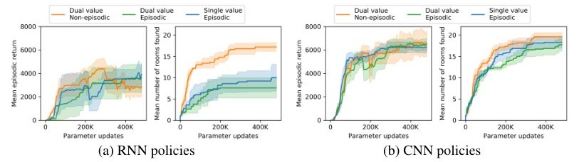
In Section 3.1 we saw that the non-episodic setting resulted in more exploration than the episodic setting when exploring without any extrinsic rewards. Next we consider whether this holds in the case where we combine intrinsic and extrinsic rewards. As discussed in Section 2.3 in order to combine episodic and non-episodic reward streams we require two value heads. This also raises the question of whether it is better to have two value heads even when both reward streams are episodic. In Figure 4 we compare episodic intrinsic rewards to non-episodic intrinsic rewards combined with episodic extrinsic rewards, and additionally two value heads versus one for the episodic case. The discount factors are $\gamma_{I}=\gamma_{E}=0.99$.

3.1 节表明：在没有任何外在奖励时，非回合制设定比回合制探索更多。接下来考察在组合内在与外在奖励时是否仍然成立。如 2.3 节所述，组合回合制与非回合制奖励流需要两个价值头。这也引出问题：即便两路奖励流都是回合制，用两个价值头是否更好。图 4 比较：非回合制内在奖励加回合制外在奖励，对回合制内在奖励；以及回合制情形下双价值头对单价值头。折扣因子为 $\gamma_{I}=\gamma_{E}=0.99$。

(a) RNN policies

(b) CNN policies

Figure 4: Different ways of combining intrinsic and extrinsic rewards. Combining non-episodic stream of intrinsic rewards with the episodic stream of extrinsic rewards outperforms combining episodic versions of both steams in terms of number of explored rooms, but performs similarly in terms of mean return. Single value estimate of the combined stream of episodic returns performs a little better than the dual value estimate. The differences are more pronounced with RNN policies. CNN runs are more stable than the RNN counterparts.

(a) RNN 策略

(b) CNN 策略

图 4：组合内在与外在奖励的不同方式。把非回合制内在奖励流与回合制外在奖励流组合，在探索房间数上优于把两者都当回合制组合，但平均回报相近。对组合的回合制回报流，单价值估计略优于双价值估计。差异在 RNN 策略上更明显。CNN 运行比对应 RNN 更稳定。

In Figure 4 we see that using a non-episodic intrinsic reward stream increases the number of rooms explored for both CNN and RNN policies, consistent with the experiments in Section 3.1, but that the difference is less dramatic, likely because the extrinsic reward is able to preserve useful behaviors. We also see that the difference is less pronounced for the CNN experiments, and that the RNN results tend to be less stable and perform worse for $\gamma_{E}=0.99$.

从图 4 可见：使用非回合制内在奖励流会增加 CNN 与 RNN 策略探索的房间数，与 3.1 节实验一致，但差异不那么剧烈，可能因为外在奖励能保留有用行为。CNN 实验上差异更小，且 RNN 结果往往更不稳定，在 $\gamma_{E}=0.99$ 时表现更差。

Contrary to our expectations (Section 2.3) using two value heads did not show any benefit over a single head in the episodic setting. Nevertheless having two value heads is necessary for combining reward streams with different characteristics, and so all further experiments use two value heads.

与我们的预期（2.3 节）相反，在回合制设定下使用两个价值头相对单头没有显示出任何好处。但要组合具有不同特性的奖励流，双价值头仍是必要的，因此后续实验全部使用双价值头。

3.3 Discount factors

3.3 折扣因子

Previous experiments (Salimans & Chen 2018; Pohlen et al. 2018; Garmulewicz et al. 2018) solving Montezuma’s Revenge using expert demonstrations used a high discount factor to achieve the best performance, enabling the agent to anticipate rewards far into the future. We compare the performance of the RND agent with $\gamma_{E}\in\{0.99,0.999\}$ and $\gamma_{I}=0.99$. We also investigate the effect of increasing $\gamma_{I}$ to 0.999. The results are shown in Figure 6.

先前用专家示范解决 Montezuma’s Revenge 的实验（Salimans & Chen 2018；Pohlen et al. 2018；Garmulewicz et al. 2018）使用高折扣因子以达最佳表现，使智能体能预见很远的未来奖励。我们比较 RND 智能体在 $\gamma_{E}\in\{0.99,0.999\}$、$\gamma_{I}=0.99$ 时的表现，并考察把 $\gamma_{I}$ 增至 0.999 的影响。结果见图 6。

In Figure 6 we see that increasing $\gamma_{E}$ to 0.999 while holding $\gamma_{I}$ at 0.99 greatly improves performance. We also see that further increasing $\gamma_{I}$ to 0.999 hurts performance. This is at odds with the results in Figure 3 where increasing $\gamma_{I}$ did not significantly impact performance.

从图 6 可见：把 $\gamma_{E}$ 增至 0.999 同时保持 $\gamma_{I}=0.99$，显著提升表现。继续把 $\gamma_{I}$ 增至 0.999 则损害表现。这与图 3 中增大 $\gamma_{I}$ 对表现影响不大的结果不一致。

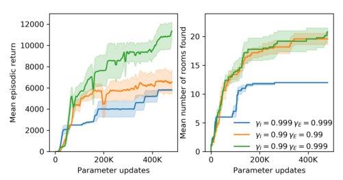
Figure 5: Performance of different discount factors for intrinsic and extrinsic reward streams. A higher discount factor for the extrinsic rewards leads to better performance, while for intrinsic rewards it hurts exploration.

图 5：内在与外在奖励流不同折扣因子的表现。外在奖励用更高折扣因子带来更好表现，而对内在奖励则会损害探索。

3.4 Scaling up training

3.4 扩大训练规模

In this section we report experiments showing the effect of increased scale on training. The intrinsic rewards are non-episodic with $\gamma_{I}=0.99$, and $\gamma_{E}=0.999$.

本节报告增大训练规模的影响。内在奖励为非回合制，$\gamma_{I}=0.99$，$\gamma_{E}=0.999$。

To hold the rate at which the intrinsic reward decreases over time constant across experiments with different numbers of parallel environments, we downsample the batch size when training the predictor to match the batch size with 32 parallel environments (for full details see Appendix A.4). Larger numbers of environments results in larger batch sizes per update for training the policy, whereas the predictor network batch size remains constant. Since the intrinsic reward disappears over time it is important for the policy to learn to find and exploit these transitory rewards, since they act as stepping-stones to nearby novel states.

为使内在奖励随时间下降的速率在不同并行环境数实验间保持不变，训练预测器时对 batch 下采样，以匹配 32 个并行环境时的 batch 大小（完整细节见附录 A.4）。更多环境意味着策略每次更新的 batch 更大，而预测网络 batch 保持不变。由于内在奖励会随时间消失，策略需要学会寻找并利用这些短暂奖励，因为它们是通往附近新颖状态的踏脚石。

Figure 6 shows that agents trained with larger batches of experience collected from more parallel environments obtain higher mean returns after similar numbers of updates. They also achieve better final performance. This effect seems to saturate earlier for the CNN policy than for the RNN policy.

图 6 表明：从更多并行环境收集更大批次经验训练的智能体，在相近更新次数后获得更高平均回报，最终表现也更好。该效应对 CNN 策略似乎比 RNN 策略更早饱和。

We allowed the RNN experiment with 32 parallel environments to run for more time, eventually reaching a mean return of 7,570 after processing 1.6 billion frames over 1.6 million parameter updates. One of these runs visited all 24 rooms, and passed the first level once, achieving a best return of 17,500. The RNN experiment with 1024 parallel environments had mean return of 10,070 at the end of training, and yielded one run with mean return of 14,415.

我们让 32 个并行环境的 RNN 实验跑更久，最终在处理 16 亿帧、160 万次参数更新后达到平均回报 7,570。其中一次运行访问了全部 24 个房间，并通关第一关一次，最佳回报 17,500。1024 个并行环境的 RNN 实验训练结束时平均回报 10,070，其中一次运行平均回报 14,415。

3.5 Recurrence

3.5 递归

Montezuma’s Revenge is a partially observable environment even though large parts of the game state can be inferred from the screen. For example the number of keys the agent has appears on the screen, but not where they come from, how many keys have been used in the past, or what doors have been opened. To deal with this partial observability, an agent should maintain a state summarizing the past, for example the state of a recurrent policy. Hence it would be natural to hope for better performance from agents with recurrent policies. Contrary to expectations in Figure 4 recurrent policies performed worse than non-recurrent counterparts with $\gamma_{E}=0.99$. However in Figure 6 the RNN policy with $\gamma_{E}=0.999$ outperformed the CNN counterpart at each scale[^1]. Comparison of Figures 7 and 9 shows that across multiple games the RNN policy outperforms the CNN more frequently than the other way around.

即便游戏状态的大部分可从屏幕推断，Montezuma’s Revenge 仍是部分可观测环境。例如智能体持有的钥匙数出现在屏幕上，但钥匙来自何处、过去用过多少钥匙、哪些门已打开则没有。为应对部分可观测性，智能体应维护总结过去的状态，例如递归策略的状态。因此自然期望递归策略表现更好。与预期相反，图 4 中在 $\gamma_{E}=0.99$ 时递归策略比非递归对应更差。但图 6 中 $\gamma_{E}=0.999$ 的 RNN 策略在各规模上都优于对应 CNN。[^1] 比较图 7 与图 9 可见：跨多个游戏，RNN 策略优于 CNN 的频率更高。

3.6 Comparison to baselines

3.6 与基线比较

In this section we compare RND to two baselines: PPO without an exploration bonus and an alternative exploration bonus based on forward dynamics error. We evaluate RND’s performance on six hard exploration Atari games: Gravitar, Montezuma’s Revenge, Pitfall!, Private Eye, Solaris, and Venture. We first compare to the performance of a baseline PPO implementation without intrinsic reward. For RND the intrinsic rewards are non-episodic with $\gamma_{I}=0.99$, while $\gamma_{E}=0.999$ for both PPO and RND. The results are shown in Figure 7 for the RNN policy and summarized in Table 1 (see also Figure 9 for the CNN policy).

本节将 RND 与两个基线比较：无探索奖励的 PPO，以及基于前向动力学误差的另一种探索奖励。我们在六个难探索 Atari 游戏上评估 RND：Gravitar、Montezuma’s Revenge、Pitfall!、Private Eye、Solaris 与 Venture。先与无内在奖励的基线 PPO 比较。对 RND，内在奖励为非回合制，$\gamma_{I}=0.99$；PPO 与 RND 的 $\gamma_{E}$ 均为 $0.999$。RNN 策略结果见图 7，汇总见表 1（CNN 策略另见图 9）。

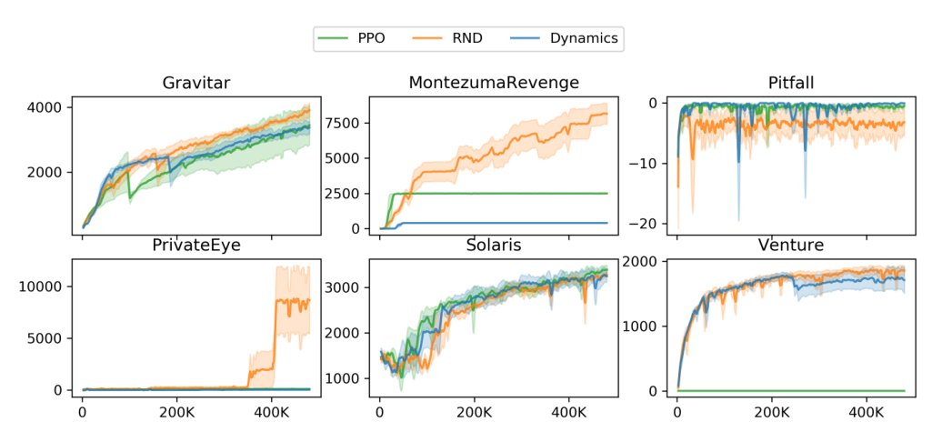
Figure 7: Mean episodic return of RNN-based policies: RND, dynamics-based exploration method, and PPO with extrinsic reward only on 6 hard exploration Atari games. RND achieves state of the art performance on Gravitar, Montezuma’s Revenge, and Venture, significantly outperforming PPO on the latter two.

图 7：基于 RNN 的策略的平均回合回报：RND、基于动力学的探索方法，以及仅用外在奖励的 PPO，在 6 个难探索 Atari 游戏上。RND 在 Gravitar、Montezuma’s Revenge 与 Venture 上达到当时最优，在后两者上显著优于 PPO。

In Gravitar we see that RND does not consistently exceed the performance of PPO. However both exceed average human performance with an RNN policy, as well as the previous state of the art. On Montezuma’s Revenge and Venture RND significantly outperforms PPO, and exceeds state of the art performance and average human performance. On Pitfall! both algorithms fail to find any positive rewards. This is a typical result for this game, as the extrinsic positive reward is very sparse. On Private Eye RND’s performance exceeds that of PPO. On Solaris RND’s performance is comparable to that of PPO.

在 Gravitar 上，RND 并未稳定地超过 PPO。但两者配合 RNN 策略都超过普通人类平均，也超过先前最优。在 Montezuma’s Revenge 与 Venture 上，RND 显著优于 PPO，并超过当时最优与普通人类平均。在 Pitfall! 上两种算法都找不到任何正奖励——对该游戏这是典型结果，因为外在正奖励非常稀疏。在 Private Eye 上 RND 优于 PPO。在 Solaris 上 RND 与 PPO 相当。

Next we consider an alternative exploration bonus based on forward dynamics error. There are numerous previous works using such a bonus (Schmidhuber 1991b; Stadie et al. 2015; Achiam & Sastry 2017; Pathak et al. 2017; Burda et al. 2018). Fortuitously Burda et al. 2018 show that training a forward dynamics model in a random feature space typically works as well as any other feature space when used to create an exploration bonus. This means that we can easily implement an apples to apples comparison and change the loss in RND so the predictor network predicts the random features of the next observation given the current observation and action, while holding fixed all other parts of our method such as dual value heads, non-episodic intrinsic returns, normalization schemes etc. This provides an ablation of the prediction problem defining the exploration bonus, while also being representative of a class of prior work using forward dynamics error. Our expectation was that these methods should be fairly similar except where the dynamics-based agent is able to exploit non-determinism in the environment to get intrinsic reward.

接下来考察基于前向动力学误差的另一种探索奖励。已有大量工作使用此类奖励（Schmidhuber 1991b；Stadie et al. 2015；Achiam & Sastry 2017；Pathak et al. 2017；Burda et al. 2018）。Burda et al. 2018 恰好表明：在随机特征空间中训练前向动力学模型，用于构造探索奖励时通常与任何其他特征空间一样好。因此我们可轻松做一对一比较：改动 RND 的损失，使预测网络根据当前观测与动作预测下一观测的随机特征，同时固定方法其余部分，如双价值头、非回合制内在回报、归一化方案等。这消融了定义探索奖励的预测问题，同时也代表使用前向动力学误差的一类先前工作。我们预期这些方法应相当接近，除非基于动力学的智能体能利用环境中的非确定性来获取内在奖励。

Figure 7 shows that dynamics-based exploration performs significantly worse than RND with the same CNN policy on Montezuma’s Revenge, PrivateEye, and Solaris, and performs similarly on Venture, Pitfall, and Gravitar. By analyzing agent’s behavior at convergence we notice that in Montezuma’s Revenge the agent oscillates between two rooms. This leads to an irreducibly high prediction error, as the non-determinism of sticky actions makes it impossible to know whether, once the agent is close to crossing a room boundary, making one extra step will result in it staying in the same room, or crossing to the next one. This is a manifestation of the ‘noisy TV’ problem, or aleatoric uncertainty discussed in Section 2.2.1. Similar behavior emerges in PrivateEye and Pitfall!. In Table 1 the final training performance for each algorithm is listed, alongside the state of the art from previous work and average human performance.

图 7 表明：在相同 CNN 策略下，基于动力学的探索在 Montezuma’s Revenge、PrivateEye 与 Solaris 上显著弱于 RND，在 Venture、Pitfall 与 Gravitar 上表现相近。分析收敛时智能体行为可见：在 Montezuma’s Revenge 中智能体在两个房间间振荡。这导致不可约的高预测误差，因为 sticky actions 的非确定性使智能体无法知道——一旦接近穿过房间边界——多走一步是留在同一房间还是进入下一房间。这正是 2.2.1 节讨论的「嘈杂电视」问题或偶然不确定性的表现。PrivateEye 与 Pitfall! 中出现类似行为。表 1 列出各算法最终训练表现，以及先前工作的当时最优与普通人类平均。

	Gravitar	Montezuma’s Revenge	Pitfall!	PrivateEye	Solaris	Venture
RND	3,906	8,152	-3	8,666	3,282	1,859
PPO	3,426	2,497	0	105	3,387	0
Dynamics	3,371	400	0	33	3,246	1,712
SOTA	2,2091	3,7002	0	15,8062	12,3801	1,8133
Avg. Human	3,351	4,753	6,464	69,571	12,327	1,188

Table 1: Comparison to baselines results. Final mean performance for various methods. State of the art results taken from: [1] (Fortunato et al. 2017) [2] (Bellemare et al. 2016) [3] (Horgan et al. 2018)

	Gravitar	Montezuma’s Revenge	Pitfall!	PrivateEye	Solaris	Venture
RND	3,906	8,152	-3	8,666	3,282	1,859
PPO	3,426	2,497	0	105	3,387	0
Dynamics	3,371	400	0	33	3,246	1,712
SOTA	2,2091	3,7002	0	15,8062	12,3801	1,8133
Avg. Human	3,351	4,753	6,464	69,571	12,327	1,188

表 1：与基线结果比较。各方法最终平均表现。当时最优结果取自：[1] (Fortunato et al. 2017) [2] (Bellemare et al. 2016) [3] (Horgan et al. 2018)

3.7 Qualitative Analysis: Dancing with skulls

3.7 定性分析：与骷髅共舞

By observing the RND agent, we notice that frequently once it obtains all the extrinsic rewards that it knows how to obtain reliably (as judged by the extrinsic value function), the agent settles into a pattern of behavior where it keeps interacting with potentially dangerous objects. For instance in Montezuma’s Revenge the agent jumps back and forth over a moving skull, moves in between laser gates, and gets on and off disappearing bridges. We also observe similar behavior in Pitfall!. It might be related to the very fact that such dangerous states are difficult to achieve, and hence are rarely represented in agent’s past experience compared to safer states.

观察 RND 智能体可见：一旦它获得了所有它知道如何可靠获得的外在奖励（由外在价值函数判断），就常常进入一种行为模式——持续与潜在危险物体交互。例如在 Montezuma’s Revenge 中，智能体在移动骷髅上反复跳来跳去、在激光门之间移动、在消失的桥上上下。Pitfall! 中也观察到类似行为。这可能与危险状态本身难以达成有关，因而相对更安全的状态，它们在智能体过往经验中出现得更少。

4 Related Work

4 相关工作

Exploration. Count-based exploration bonuses are a natural and effective way to do exploration (Strehl & Littman 2008) and a lot of work has studied how to tractably generalize count bonuses to large state spaces (Bellemare et al. 2016; Fu et al. 2017; Ostrovski et al. 2017; Tang et al. 2017; Machado et al. 2018; Fox et al. 2018).

探索。 基于计数的探索奖励是做探索的自然且有效方式（Strehl & Littman 2008），大量工作研究如何把计数奖励可扩展地推广到大状态空间（Bellemare et al. 2016；Fu et al. 2017；Ostrovski et al. 2017；Tang et al. 2017；Machado et al. 2018；Fox et al. 2018）。

Another class of exploration methods rely on errors in predicting dynamics (Schmidhuber 1991b; Stadie et al. 2015; Achiam & Sastry 2017; Pathak et al. 2017; Burda et al. 2018). As discussed in Section 2.2, these methods are subject to the ‘noisy TV’ problem in stochastic or partially-observable environments. This has motivated work on exploration via quantification of uncertainty (Still & Precup 2012; Houthooft et al. 2016) or prediction improvement measures (Schmidhuber 1991a; Oudeyer et al. 2007; Lopes et al. 2012; Achiam & Sastry 2017).

另一类探索方法依赖预测动力学的误差（Schmidhuber 1991b；Stadie et al. 2015；Achiam & Sastry 2017；Pathak et al. 2017；Burda et al. 2018）。如 2.2 节所述，这些方法在随机或部分可观测环境中受「嘈杂电视」问题影响。这促使人们研究通过量化不确定性（Still & Precup 2012；Houthooft et al. 2016）或预测改进度量（Schmidhuber 1991a；Oudeyer et al. 2007；Lopes et al. 2012；Achiam & Sastry 2017）来做探索。

Other methods of exploration include adversarial self-play (Sukhbaatar et al. 2018), maximizing empowerment (Gregor et al. 2017), parameter noise (Plappert et al. 2017; Fortunato et al. 2017), identifying diverse policies (Eysenbach et al. 2018; Achiam et al. 2018), and using ensembles of value functions (Osband et al. 2018; Osband et al. 2016; Chen et al. 2017).

其他探索方法包括对抗自对弈（Sukhbaatar et al. 2018）、最大化赋权（Gregor et al. 2017）、参数噪声（Plappert et al. 2017；Fortunato et al. 2017）、识别多样策略（Eysenbach et al. 2018；Achiam et al. 2018），以及使用价值函数集成（Osband et al. 2018；Osband et al. 2016；Chen et al. 2017）。

Montezuma’s Revenge. Early neural-network based reinforcement learning algorithms that were successful on a significant portion of Atari games (Mnih et al. 2015; Mnih et al. 2016; Hessel et al. 2017) failed to make meaningful progress on Montezuma’s Revenge, not finding a way out of the first room reliably. This is not necessarily a failure of exploration, as even a random agent finds the key in the first room once every few hundred thousand steps, and escapes the first room every few million steps. Indeed, a mean return of about 2,500 can be reliably achieved without special exploration methods (Horgan et al. 2018; Espeholt et al. 2018; Oh et al. 2018).

Montezuma’s Revenge。 早期在相当一部分 Atari 游戏上成功的基于神经网络的强化学习算法（Mnih et al. 2015；Mnih et al. 2016；Hessel et al. 2017）未能在 Montezuma’s Revenge 上取得有意义进展，甚至无法可靠找到离开第一个房间的方法。这未必是探索失败：即便随机智能体也能每几十万步在第一房间找到钥匙，每几百万步逃出第一房间。实际上，平均回报约 2,500 可在无特殊探索方法时可靠达到（Horgan et al. 2018；Espeholt et al. 2018；Oh et al. 2018）。

Combining DQN with a pseudo-count exploration bonus Bellemare et al. 2016 set a new state of the art performance, exploring 15 rooms and getting best return of 6,600. Since then a number of other works have achieved similar performance (O’Donoghue et al. 2017; Ostrovski et al. 2018; Machado et al. 2018; Osband et al. 2018), without exceeding it.

把 DQN 与伪计数探索奖励结合，Bellemare et al. 2016 刷新了当时最优，探索 15 个房间，最佳回报 6,600。此后若干工作达到类似表现（O’Donoghue et al. 2017；Ostrovski et al. 2018；Machado et al. 2018；Osband et al. 2018），但未超越。

Special access to the underlying RAM state can also be used to improve exploration by using it to hand-craft exploration bonuses (Kulkarni et al. 2016; Tang et al. 2017; Stanton & Clune 2018). Even with such access previous work achieves performance inferior to average human performance.

特殊访问底层 RAM 状态也可用于改进探索，借此手工设计探索奖励（Kulkarni et al. 2016；Tang et al. 2017；Stanton & Clune 2018）。即便有这种访问，先前工作的表现仍低于普通人类平均。

Expert demonstrations can be used effectively to simplify the exploration problem in Montezuma’s Revenge, and a number of works (Salimans & Chen 2018; Pohlen et al. 2018; Aytar et al. 2018; Garmulewicz et al. 2018) have achieved performance comparable to or better than that of human experts. Learning from expert demonstrations benefits from the game’s determinism. The suggested training method (Machado et al. 2017) to prevent an agent from simply memorizing the correct sequence of actions is to use sticky actions (i.e. randomly repeating previous action) has not been used in these works. In this work we use sticky actions and thus don’t rely on determinism.

专家示范可有效简化 Montezuma’s Revenge 中的探索问题，若干工作（Salimans & Chen 2018；Pohlen et al. 2018；Aytar et al. 2018；Garmulewicz et al. 2018）达到可比或优于人类专家的表现。从专家示范学习受益于游戏的确定性。为防止智能体简单记忆正确动作序列，Machado et al. 2017 建议使用 sticky actions（随机重复上一动作），但这些工作未采用。本文使用 sticky actions，因而不依赖确定性。

Random features. Features of randomly initialized neural networks have been extensively studied in the context of supervised learning (Rahimi & Recht 2008; Saxe et al. 2011; Jarrett et al. 2009; Yang et al. 2015). More recently they have been used in the context of exploration (Osband et al. 2018; Burda et al. 2018). The work Osband et al. 2018 provides motivation for random network distillation as discussed in Section 2.2.

随机特征。 随机初始化神经网络的特征在监督学习语境下被广泛研究（Rahimi & Recht 2008；Saxe et al. 2011；Jarrett et al. 2009；Yang et al. 2015）。近期也被用于探索（Osband et al. 2018；Burda et al. 2018）。Osband et al. 2018 为随机网络蒸馏提供了动机，见 2.2 节。

Vectorized value functions. Pong et al. 2018 find that a vectorized value function (with coordinates corresponding to additive factors of the reward) improves their method. Bellemare et al. 2017 parametrize the value as a linear combination of value heads that estimate probabilities of discretized returns. However the Bellman backup equation used there is not itself vectorized.

向量化价值函数。 Pong et al. 2018 发现向量化价值函数（坐标对应奖励的加性因子）能改进其方法。Bellemare et al. 2017 把价值参数化为估计离散化回报概率的价值头的线性组合。但那里使用的 Bellman 备份方程本身并非向量化。

5 Discussion

5 讨论

This paper introduced an exploration method based on random network distillation and experimentally showed that the method is capable of performing directed exploration on several Atari games with very sparse rewards. These experiments suggest that progress on hard exploration games is possible with relatively simple generic methods, especially when applied at scale. They also suggest that methods that are able to treat the stream of intrinsic rewards separately from the stream of extrinsic rewards (for instance by having separate value heads) can benefit from such flexibility.

本文引入基于随机网络蒸馏的探索方法，并实验表明该方法能在若干奖励极稀疏的 Atari 游戏上做有向探索。这些实验表明：即便相对简单的通用方法——尤其在规模化应用时——也能在难探索游戏上取得进展。它们还表明：能把内在奖励流与外在奖励流分开处理的方法（例如使用分离的价值头）可以从这种灵活性中受益。

We find that the RND exploration bonus is sufficient to deal with local exploration, i.e. exploring the consequences of short-term decisions, like whether to interact with a particular object, or avoid it. However global exploration that involves coordinated decisions over long time horizons is beyond the reach of our method.

我们发现 RND 探索奖励足以应对局部探索，即探索短期决策的后果，例如是否与某个物体交互或避开它。但涉及长时程协调决策的全局探索，超出了本方法的能力。

To solve the first level of Montezuma’s Revenge, the agent must enter a room locked behind two doors. There are four keys and six doors spread throughout the level. Any of the four keys can open any of the six doors, but are consumed in the process. To open the final two doors the agent must therefore forego opening two of the doors that are easier to find and that would immediately reward it for opening them.

要通关 Montezuma’s Revenge 第一关，智能体必须进入锁在两扇门后的房间。关卡中散布四把钥匙与六扇门。任意钥匙可开任意门，但开后即消耗。因此要打开最后两扇门，智能体必须放弃打开两扇更容易找到、且打开后能立即给奖励的门。

To incentivize this behavior the agent should receive enough intrinsic reward for saving the keys to balance the loss of extrinsic reward from using them early on. From our analysis of the RND agent’s behavior, it does not get a large enough incentive to try this strategy, and only stumbles upon it rarely.

要激励这种行为，智能体应为节省钥匙获得足够内在奖励，以平衡过早用钥匙损失的外在奖励。从对 RND 智能体行为的分析看，它并未获得足够激励去尝试该策略，只是偶尔偶然撞上。

Solving this and similar problems that require high level exploration is an important direction for future work.

解决这类需要高层探索的问题，是未来工作的重要方向。

References

参考文献

Achiam & Sastry (2017) Joshua Achiam and Shankar Sastry. Surprise-based intrinsic motivation for deep reinforcement learning. arXiv:1703.01732 , 2017.

Achiam et al. (2018) Joshua Achiam, Harrison Edwards, Dario Amodei, and Pieter Abbeel. Variational option discovery algorithms. arXiv preprint arXiv:1807.10299 , 2018.

Aytar et al. (2018) Yusuf Aytar, Tobias Pfaff, David Budden, Tom Le Paine, Ziyu Wang, and Nando de Freitas. Playing hard exploration games by watching YouTube. arXiv preprint arXiv:1805.11592 , 2018.

Bellemare et al. (2016) Marc Bellemare, Sriram Srinivasan, Georg Ostrovski, Tom Schaul, David Saxton, and Remi Munos. Unifying count-based exploration and intrinsic motivation. In NIPS , 2016.

Bellemare et al. (2017) Marc G Bellemare, Will Dabney, and Rémi Munos. A distributional perspective on reinforcement learning. arXiv preprint arXiv:1707.06887 , 2017.

Burda et al. (2018) Yuri Burda, Harri Edwards, Deepak Pathak, Amos Storkey, Trevor Darrell, and Alexei A. Efros. Large-scale study of curiosity-driven learning. In arXiv:1808.04355 , 2018.

Chen et al. (2017) Richard Y Chen, John Schulman, Pieter Abbeel, and Szymon Sidor. UCB and infogain exploration via q q -ensembles. arXiv:1706.01502 , 2017.

Cho et al. (2014) Kyunghyun Cho, Bart Van Merriënboer, Caglar Gulcehre, Dzmitry Bahdanau, Fethi Bougares, Holger Schwenk, and Yoshua Bengio. Learning phrase representations using RNN encoder-decoder for statistical machine translation. arXiv preprint arXiv:1406.1078 , 2014.

Denil et al. (2016) Misha Denil, Pulkit Agrawal, Tejas D Kulkarni, Tom Erez, Peter Battaglia, and Nando de Freitas. Learning to perform physics experiments via deep reinforcement learning. arXiv preprint arXiv:1611.01843 , 2016.

Espeholt et al. (2018) Lasse Espeholt, Hubert Soyer, Remi Munos, Karen Simonyan, Volodymir Mnih, Tom Ward, Yotam Doron, Vlad Firoiu, Tim Harley, Iain Dunning, et al. IMPALA: Scalable distributed Deep-RL with importance weighted actor-learner architectures. arXiv preprint arXiv:1802.01561 , 2018.

Eysenbach et al. (2018) Benjamin Eysenbach, Abhishek Gupta, Julian Ibarz, and Sergey Levine. Diversity is all you need: Learning skills without a reward function. arXiv preprint , 2018.

Fortunato et al. (2017) Meire Fortunato, Mohammad Gheshlaghi Azar, Bilal Piot, Jacob Menick, Ian Osband, Alex Graves, Vlad Mnih, Remi Munos, Demis Hassabis, Olivier Pietquin, Charles Blundell, and Shane Legg. Noisy networks for exploration. arXiv:1706.10295 , 2017.

Fox et al. (2018) Lior Fox, Leshem Choshen, and Yonatan Loewenstein. Dora the explorer: Directed outreaching reinforcement action-selection. International Conference on Learning Representations , 2018.

Fu et al. (2017) Justin Fu, John D Co-Reyes, and Sergey Levine. EX2: Exploration with exemplar models for deep reinforcement learning. NIPS , 2017.

Garmulewicz et al. (2018) Michał Garmulewicz, Henryk Michalewski, and Piotr Miłoś. Expert-augmented actor-critic for vizdoom and montezumas revenge. arXiv preprint arXiv:1809.03447 , 2018.

Gregor et al. (2017) Karol Gregor, Danilo Jimenez Rezende, and Daan Wierstra. Variational intrinsic control. ICLR Workshop , 2017.

Haber et al. (2018) Nick Haber, Damian Mrowca, Li Fei-Fei, and Daniel LK Yamins. Learning to play with intrinsically-motivated self-aware agents. arXiv preprint arXiv:1802.07442 , 2018.

Hessel et al. (2017) Matteo Hessel, Joseph Modayil, Hado Van Hasselt, Tom Schaul, Georg Ostrovski, Will Dabney, Dan Horgan, Bilal Piot, Mohammad Azar, and David Silver. Rainbow: Combining improvements in deep reinforcement learning. arXiv preprint arXiv:1710.02298 , 2017.

Horgan et al. (2018) Dan Horgan, John Quan, David Budden, Gabriel Barth-Maron, Matteo Hessel, Hado Van Hasselt, and David Silver. Distributed prioritized experience replay. arXiv preprint arXiv:1803.00933 , 2018.

Houthooft et al. (2016) Rein Houthooft, Xi Chen, Yan Duan, John Schulman, Filip De Turck, and Pieter Abbeel. VIME: Variational information maximizing exploration. In NIPS , 2016.

Jarrett et al. (2009) Kevin Jarrett, Koray Kavukcuoglu, Yann LeCun, et al. What is the best multi-stage architecture for object recognition? In Computer Vision, 2009 IEEE 12th International Conference on , pp. 2146–2153. IEEE, 2009.

Kingma & Ba (2015) Diederik Kingma and Jimmy Ba. Adam: A method for stochastic optimization. ICLR , 2015.

Kulkarni et al. (2016) Tejas D Kulkarni, Karthik Narasimhan, Ardavan Saeedi, and Josh Tenenbaum. Hierarchical deep reinforcement learning: Integrating temporal abstraction and intrinsic motivation. In Advances in neural information processing systems , pp. 3675–3683, 2016.

Lopes et al. (2012) Manuel Lopes, Tobias Lang, Marc Toussaint, and Pierre-Yves Oudeyer. Exploration in model-based reinforcement learning by empirically estimating learning progress. In NIPS , 2012.

Machado et al. (2017) Marlos C Machado, Marc G Bellemare, Erik Talvitie, Joel Veness, Matthew Hausknecht, and Michael Bowling. Revisiting the arcade learning environment: Evaluation protocols and open problems for general agents. arXiv preprint arXiv:1709.06009 , 2017.

Machado et al. (2018) Marlos C Machado, Marc G Bellemare, and Michael Bowling. Count-based exploration with the successor representation. arXiv preprint arXiv:1807.11622 , 2018.

Mnih et al. (2013) Volodymyr Mnih, Koray Kavukcuoglu, David Silver, Alex Graves, Ioannis Antonoglou, Daan Wierstra, and Martin Riedmiller. Playing Atari with deep reinforcement learning. arXiv preprint arXiv:1312.5602 , 2013.

Mnih et al. (2015) Volodymyr Mnih, Koray Kavukcuoglu, David Silver, Andrei A. Rusu, Joel Veness, Marc G. Bellemare, Alex Graves, Martin Riedmiller, Andreas K. Fidjeland, Georg Ostrovski, Stig Petersen, Charles Beattie, Amir Sadik, Ioannis Antonoglou, Helen King, Dharshan Kumaran, Daan Wierstra, Shane Legg, and Demis Hassabis. Human-level control through deep reinforcement learning. Nature , 518(7540):529–533, February 2015.

Mnih et al. (2016) Volodymyr Mnih, Adria Puigdomenech Badia, Mehdi Mirza, Alex Graves, Timothy Lillicrap, Tim Harley, David Silver, and Koray Kavukcuoglu. Asynchronous methods for deep reinforcement learning. In ICML , 2016.

O’Donoghue et al. (2017) Brendan O’Donoghue, Ian Osband, Remi Munos, and Volodymyr Mnih. The uncertainty Bellman equation and exploration. arXiv preprint arXiv:1709.05380 , 2017.

Oh et al. (2018) Junhyuk Oh, Yijie Guo, Satinder Singh, and Honglak Lee. Self-imitation learning. arXiv preprint arXiv:1806.05635 , 2018.

OpenAI (2018) OpenAI. OpenAI Five. https://blog.openai.com/openai-five/ , 2018.

OpenAI et al. (2018) OpenAI, :, M. Andrychowicz, B. Baker, M. Chociej, R. Jozefowicz, B. McGrew, J. Pachocki, A. Petron, M. Plappert, G. Powell, A. Ray, J. Schneider, S. Sidor, J. Tobin, P. Welinder, L. Weng, and W. Zaremba. Learning Dexterous In-Hand Manipulation. ArXiv e-prints , August 2018.

Osband et al. (2016) Ian Osband, Charles Blundell, Alexander Pritzel, and Benjamin Van Roy. Deep exploration via bootstrapped DQN. In NIPS , 2016.

Osband et al. (2018) Ian Osband, John Aslanides, and Albin Cassirer. Randomized prior functions for deep reinforcement learning. arXiv preprint arXiv:1806.03335 , 2018.

Ostrovski et al. (2017) Georg Ostrovski, Marc G Bellemare, Aaron van den Oord, and Rémi Munos. Count-based exploration with neural density models. arXiv:1703.01310 , 2017.

Ostrovski et al. (2018) Georg Ostrovski, Marc G Bellemare, Aaron van den Oord, and Rémi Munos. Count-based exploration with neural density models. International Conference for Machine Learning , 2018.

Oudeyer et al. (2007) Pierre-Yves Oudeyer, Frdric Kaplan, and Verena V Hafner. Intrinsic motivation systems for autonomous mental development. Evolutionary Computation , 2007.

Pathak et al. (2017) Deepak Pathak, Pulkit Agrawal, Alexei A. Efros, and Trevor Darrell. Curiosity-driven exploration by self-supervised prediction. In ICML , 2017.

Plappert et al. (2017) Matthias Plappert, Rein Houthooft, Prafulla Dhariwal, Szymon Sidor, Richard Y Chen, Xi Chen, Tamim Asfour, Pieter Abbeel, and Marcin Andrychowicz. Parameter space noise for exploration. arXiv:1706.01905 , 2017.

Pohlen et al. (2018) Tobias Pohlen, Bilal Piot, Todd Hester, Mohammad Gheshlaghi Azar, Dan Horgan, David Budden, Gabriel Barth-Maron, Hado van Hasselt, John Quan, Mel Večerík, et al. Observe and look further: Achieving consistent performance on Atari. arXiv preprint arXiv:1805.11593 , 2018.

Pong et al. (2018) Vitchyr Pong, Shixiang Gu, Murtaza Dalal, and Sergey Levine. Temporal difference models: Model-free deep RL for model-based control. arXiv preprint arXiv:1802.09081 , 2018.

Rahimi & Recht (2008) Ali Rahimi and Benjamin Recht. Random features for large-scale kernel machines. In Advances in neural information processing systems , pp. 1177–1184, 2008.

Salimans & Chen (2018) Tim Salimans and Richard Chen. Learning Montezuma’s Revenge from a single demonstration. https://blog.openai.com/learning-montezumas-revenge-from-a-single-demonstration/ , 2018.

Saxe et al. (2011) Andrew M Saxe, Pang Wei Koh, Zhenghao Chen, Maneesh Bhand, Bipin Suresh, and Andrew Y Ng. On random weights and unsupervised feature learning. In ICML , pp. 1089–1096, 2011.

Schmidhuber (1991a) Jürgen Schmidhuber. Curious model-building control systems. In Neural Networks, 1991. 1991 IEEE International Joint Conference on , pp. 1458–1463. IEEE, 1991a.

Schmidhuber (1991b) Jürgen Schmidhuber. A possibility for implementing curiosity and boredom in model-building neural controllers. In Proceedings of the First International Conference on Simulation of Adaptive Behavior , 1991b.

Schulman et al. (2017) John Schulman, Filip Wolski, Prafulla Dhariwal, Alec Radford, and Oleg Klimov. Proximal policy optimization algorithms. arXiv preprint arXiv:1707.06347 , 2017.

Silver et al. (2016) David Silver, Aja Huang, Chris J. Maddison, Arthur Guez, Laurent Sifre, George van den Driessche, Julian Schrittwieser, Ioannis Antonoglou, Veda Panneershelvam, Marc Lanctot, Sander Dieleman, Dominik Grewe, John Nham, Nal Kalchbrenner, Ilya Sutskever, Timothy Lillicrap, Madeleine Leach, Koray Kavukcuoglu, Thore Graepel, and Demis Hassabis. Mastering the game of Go with deep neural networks and tree search. Nature , 529(7587):484–489, Jan 2016. ISSN 0028-0836. doi: 10.1038/nature16961 .

Stadie et al. (2015) Bradly C Stadie, Sergey Levine, and Pieter Abbeel. Incentivizing exploration in reinforcement learning with deep predictive models. NIPS Workshop , 2015.

Stanton & Clune (2018) Christopher Stanton and Jeff Clune. Deep curiosity search: Intra-life exploration improves performance on challenging deep reinforcement learning problems. arXiv preprint arXiv:1806.00553 , 2018.

Still & Precup (2012) Susanne Still and Doina Precup. An information-theoretic approach to curiosity-driven reinforcement learning. Theory in Biosciences , 2012.

Strehl & Littman (2008) Alexander L Strehl and Michael L Littman. An analysis of model-based interval estimation for markov decision processes. Journal of Computer and System Sciences , 74(8):1309–1331, 2008.

Sukhbaatar et al. (2018) Sainbayar Sukhbaatar, Ilya Kostrikov, Arthur Szlam, and Rob Fergus. Intrinsic motivation and automatic curricula via asymmetric self-play. In ICLR , 2018.

Tang et al. (2017) Haoran Tang, Rein Houthooft, Davis Foote, Adam Stooke, Xi Chen, Yan Duan, John Schulman, Filip DeTurck, and Pieter Abbeel. # exploration: A study of count-based exploration for deep reinforcement learning. In NIPS , 2017.

Yang et al. (2015) Zichao Yang, Marcin Moczulski, Misha Denil, Nando de Freitas, Alex Smola, Le Song, and Ziyu Wang. Deep fried convnets. In Proceedings of the IEEE International Conference on Computer Vision , pp. 1476–1483, 2015.

Zoph & Le (2016) Barret Zoph and Quoc V Le. Neural architecture search with reinforcement learning. arXiv preprint arXiv:1611.01578 , 2016.

Appendix A Appendix

附录 A 附录

A.1 Reinforcement Learning Algorithm

A.1 强化学习算法

An exploration bonus can be used with any RL algorithm by modifying the rewards used to train the model (i.e., $r_{t}=i_{t}+e_{t}$). We combine our proposed exploration bonus with a baseline reinforcement learning algorithm PPO (Schulman et al. 2017). PPO is a policy gradient method that we have found to require little tuning for good performance. For algorithmic details see Algorithm 1.

探索奖励可通过修改训练模型所用的奖励（即 $r_{t}=i_{t}+e_{t}$）与任意 RL 算法合用。我们将所提探索奖励与基线强化学习算法 PPO（Schulman et al. 2017）结合。PPO 是一种策略梯度方法，我们发现它几乎不需调参即可有良好表现。算法细节见算法 1。

A.2 RND Pseudo-code

A.2 RND 伪代码

Algorithm 1 gives an overall picture of the RND method. Exact details of the method can be found in the code accompanying this paper.

算法 1 给出 RND 方法的整体图景。方法的精确细节见本文附带代码。

$N\leftarrow$ number of rollouts
$N_{\text{opt}}\leftarrow$ number of optimization steps
$K\leftarrow$ length of rollout
$M\leftarrow$ number of initial steps for initializing observation normalization
$t=0$
Sample state $s_{0}\sim p_{0}(s_{0})$
for $m=1$ to $M$ do
sample $a_{t}\sim\text{Uniform}(a_{t})$
sample $s_{t+1}\sim p(s_{t+1}|s_{t},a_{t})$
Update observation normalization parameters using $s_{t+1}$
t += 1
end for
for $i=1$ to $N$ do
for $j=1$ to $K$ do
sample $a_{t}\sim\pi(a_{t}|s_{t})$
sample $s_{t+1},e_{t}\sim p(s_{t+1},e_{t}|s_{t},a_{t})$
calculate intrinsic reward $i_{t}=\lVert\hat{f}(s_{t+1})-f(s_{t+1})\rVert^{2}$
add $s_{t},s_{t+1},a_{t},e_{t},i_{t}$ to optimization batch $B_{i}$
Update reward normalization parameters using $i_{t}$
t += 1
end for
Normalize the intrinsic rewards contained in $B_{i}$
Calculate returns $R_{I,i}$ and advantages $A_{I,i}$ for intrinsic reward
Calculate returns $R_{E,i}$ and advantages $A_{E,i}$ for extrinsic reward
Calculate combined advantages $A_{i}=A_{I,i}+A_{E,i}$
Update observation normalization parameters using $B_{i}$
for $j=1$ to $N_{\text{opt}}$ do
optimize $\theta_{\pi}$ wrt PPO loss on batch $B_{i},R_{i},A_{i}$ using Adam
optimize $\theta_{\hat{f}}$ wrt distillation loss on $B_{i}$ using Adam
end for
end for

Algorithm 1 RND pseudo-code

$N\leftarrow$ number of rollouts
$N_{\text{opt}}\leftarrow$ number of optimization steps
$K\leftarrow$ length of rollout
$M\leftarrow$ number of initial steps for initializing observation normalization
$t=0$
Sample state $s_{0}\sim p_{0}(s_{0})$
for $m=1$ to $M$ do
sample $a_{t}\sim\text{Uniform}(a_{t})$
sample $s_{t+1}\sim p(s_{t+1}|s_{t},a_{t})$
Update observation normalization parameters using $s_{t+1}$
t += 1
end for
for $i=1$ to $N$ do
for $j=1$ to $K$ do
sample $a_{t}\sim\pi(a_{t}|s_{t})$
sample $s_{t+1},e_{t}\sim p(s_{t+1},e_{t}|s_{t},a_{t})$
calculate intrinsic reward $i_{t}=\lVert\hat{f}(s_{t+1})-f(s_{t+1})\rVert^{2}$
add $s_{t},s_{t+1},a_{t},e_{t},i_{t}$ to optimization batch $B_{i}$
Update reward normalization parameters using $i_{t}$
t += 1
end for
Normalize the intrinsic rewards contained in $B_{i}$
Calculate returns $R_{I,i}$ and advantages $A_{I,i}$ for intrinsic reward
Calculate returns $R_{E,i}$ and advantages $A_{E,i}$ for extrinsic reward
Calculate combined advantages $A_{i}=A_{I,i}+A_{E,i}$
Update observation normalization parameters using $B_{i}$
for $j=1$ to $N_{\text{opt}}$ do
optimize $\theta_{\pi}$ wrt PPO loss on batch $B_{i},R_{i},A_{i}$ using Adam
optimize $\theta_{\hat{f}}$ wrt distillation loss on $B_{i}$ using Adam
end for
end for

算法 1 RND 伪代码

A.3 Preprocessing details

A.3 预处理细节

Table 2 contains details of how we preprocessed the environment for our experiments. We followed the recommendations in Machado et al. 2017 in using sticky actions in order to make the environments non-deterministic so that memorization of action sequences is not possible. In Table 4 we show additional preprocessing details for the policy and value networks. In Table 4 we show additional preprocessing details for the predictor and target networks.

表 2 给出实验中如何预处理环境的细节。我们遵循 Machado et al. 2017 的建议使用 sticky actions，使环境非确定，从而无法记忆动作序列。表 4 给出策略与价值网络的额外预处理细节。表 4 也给出预测器与目标网络的额外预处理细节。

Hyperparameter	Value
Grey-scaling	True
Observation downsampling	(84,84)
Extrinsic reward clipping	$[-1,1]$
Intrinsic reward clipping	False
Max frames per episode	18K
Terminal on loss of life	False
Max and skip frames	4
Random starts	False
Sticky action probability	0.25

Table 2: Preprocessing details for the environments for all experiments.

Hyperparameter	Value
Grey-scaling	True
Observation downsampling	(84,84)
Extrinsic reward clipping	$[-1,1]$
Intrinsic reward clipping	False
Max frames per episode	18K
Terminal on loss of life	False
Max and skip frames	4
Random starts	False
Sticky action probability	0.25

表 2：所有实验的环境预处理细节。

Hyperparameter	Value
Frames stacked	4
Observation	$x\mapsto x/255$
normalization

Hyperparameter	Value
Frames stacked	1
Observation	$x\mapsto\text{CLIP}\left((x-\mu)/\sigma,[-5,5]\right)$
normalization

Table 3: Preprocessing details for policy and value network for all experiments.

Hyperparameter	Value
Frames stacked	4
Observation	$x\mapsto x/255$
normalization

Hyperparameter	Value
Frames stacked	1
Observation	$x\mapsto\text{CLIP}\left((x-\mu)/\sigma,[-5,5]\right)$
normalization

表 3：所有实验中策略与价值网络的预处理细节。

A.4 PPO and RND hyperparameters

A.4 PPO 与 RND 超参数

In Table 5 the hyperparameters for the PPO RL algorithm along with any additional hyperparameters used for RND are shown. Complete details for how these hyperparameters are used can be found in the code accompanying this paper.

表 5 给出 PPO RL 算法的超参数以及 RND 使用的任何额外超参数。这些超参数如何使用的完整细节见本文附带代码。

Hyperparameter	Value
Rollout length	128
Total number of rollouts per environment	30K
Number of minibatches	4
Number of optimization epochs	4
Coefficient of extrinsic reward	2
Coefficient of intrinsic reward	1
Number of parallel environments	128
Learning rate	$0.0001$
Optimization algorithm	Adam (Kingma & Ba 2015)
$\lambda$	0.95
Entropy coefficient	0.001
Proportion of experience used for training predictor	0.25
$\gamma_{E}$	0.999
$\gamma_{I}$	0.99
Clip range	$[0.9,1.1]$
Policy architecture	CNN

Table 5: Default hyperparameters for PPO and RND algorithms for experiments where applicable. Any differences to these defaults are detailed in the main text.

Hyperparameter	Value
Rollout length	128
Total number of rollouts per environment	30K
Number of minibatches	4
Number of optimization epochs	4
Coefficient of extrinsic reward	2
Coefficient of intrinsic reward	1
Number of parallel environments	128
Learning rate	$0.0001$
Optimization algorithm	Adam (Kingma & Ba 2015)
$\lambda$	0.95
Entropy coefficient	0.001
Proportion of experience used for training predictor	0.25
$\gamma_{E}$	0.999
$\gamma_{I}$	0.99
Clip range	$[0.9,1.1]$
Policy architecture	CNN

表 5：适用实验中 PPO 与 RND 算法的默认超参数。与这些默认值的任何差异在正文中详述。

Initial preliminary experiments with RND were run with only 32 parallel environments. We expected that increasing the number of parallel environments would improve performance by allowing the policy to adapt more quickly to transient intrinsic rewards. This effect could have been mitigated however if the predictor network also learned more quickly. To avoid this situation when scaling up from 32 to 128 environments we kept the effective batch size for the predictor network the same by randomly dropping out elements of the batch with keep probability $0.25$. Similarly in our experiments with 256 and 1,024 environments we dropped experience for the predictor with respective probabilities $0.125$ and $0.03125$.

RND 的初步实验仅用 32 个并行环境。我们预期增加并行环境数会改善表现，使策略能更快适配短暂的内在奖励。但若预测网络也学得更快，该效应可能被削弱。为避免从 32 扩到 128 个环境时出现这种情况，我们通过以保留概率 $0.25$ 随机丢弃 batch 元素，使预测网络的有效 batch 大小保持不变。类似地，在 256 与 1,024 个环境的实验中，我们分别以概率 $0.125$ 与 $0.03125$ 丢弃预测器用的经验。

A.5 Architectures

A.5 架构

In this paper we use two policy architectures: an RNN and a CNN. Both contain convolutional encoders identical of those in the standard architecture from (Mnih et al. 2015). The RNN architecture additionally contains GRU (Cho et al. 2014) cells to capture longer contexts. The layer sizes of the policies were chosen so that the number of parameters matches closely. The architectures of the target and predictor networks also have convolutional encoders identical to the ones in (Mnih et al. 2015) followed by dense layers. Exact details are given in the code accompanying this paper.

本文使用两种策略架构：RNN 与 CNN。二者都含与 (Mnih et al. 2015) 标准架构相同的卷积编码器。RNN 架构额外含 GRU（Cho et al. 2014）单元以捕捉更长上下文。策略的层大小选择使参数量接近匹配。目标与预测网络的架构也有与 (Mnih et al. 2015) 相同的卷积编码器，后接稠密层。精确细节见本文附带代码。

A.6 Additional experimental results

A.6 额外实验结果

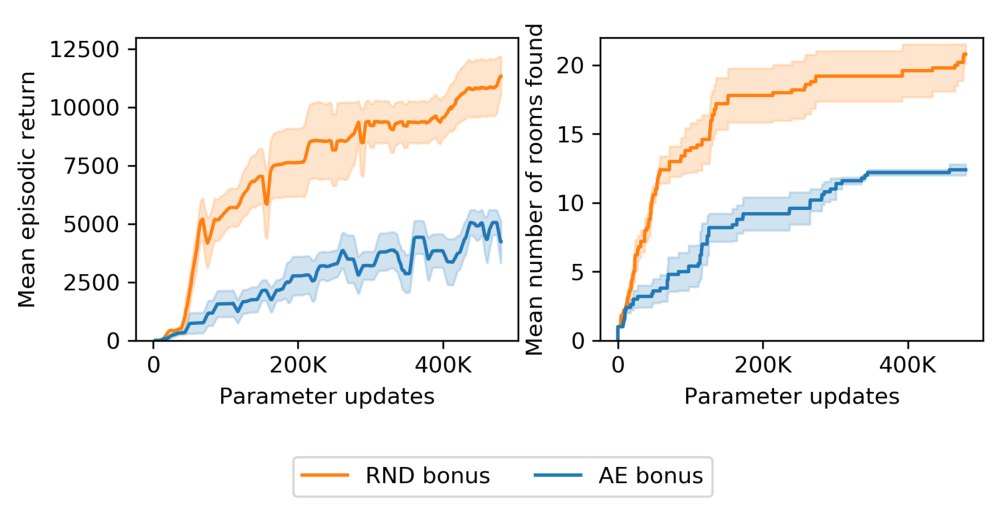
Figure 8: Comparison of RND with a CNN policy with $\gamma_{I}=0.99$ and $\gamma_{E}=0.999$ with an exploration defined by the reconstruction error of an autoencoder, holding all other choices constant (e.g. using dual value, treating intrinsic return as non-episodic etc). The performance of the autoencoder-based agent is worse than that of RND, but exceeds that of baseline PPO.

图 8：将 $\gamma_{I}=0.99$、$\gamma_{E}=0.999$ 的 CNN 策略 RND，与用自编码器重构误差定义探索、其余选择保持不变（例如使用双价值、把内在回报当非回合制等）的方法比较。基于自编码器的智能体表现弱于 RND，但超过基线 PPO。

Figure 8 compares the performance of RND with an identical algorithm, but with the exploration bonus defined as the reconstruction error of an autoencoder. The autoencoding task is similar in nature to the random network distillation, as it also obviates the second (though not necessarily the third) sources of prediction error from section 2.2.1. The experiment shows that the autoencoding task can also be successfully used for exploration.

图 8 将 RND 与算法相同、但探索奖励定义为自编码器重构误差的方法比较。自编码任务与随机网络蒸馏性质相似，因为它也消解了 2.2.1 节预测误差来源中的第二项（虽不一定消解第三项）。实验表明自编码任务也可成功用于探索。

Figure 9 compares the performance of RND to PPO and dynamics prediction-based baselines for CNN policies.

图 9 比较 CNN 策略下 RND 与 PPO、基于动力学预测的基线的表现。

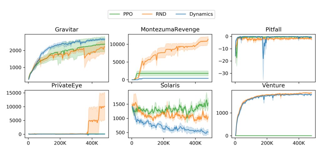
Figure 9: Mean episodic return of CNN-based policies: RND, dynamics-based exploration method, and PPO with extrinsic reward only on 6 hard exploration Atari games. RND significantly outperforms PPO on Montezuma’s Revenge, Private Eye, and Venture.

图 9：基于 CNN 的策略的平均回合回报：RND、基于动力学的探索方法，以及仅用外在奖励的 PPO，在 6 个难探索 Atari 游戏上。RND 在 Montezuma’s Revenge、Private Eye 与 Venture 上显著优于 PPO。

A.7 Additional Experimental Details

A.7 额外实验细节

In Table 6 we show the number of seeds used for each experiment, indexed by figure.

表 6 给出各实验使用的种子数，按图编号索引。

Figure number	Number of seeds
1	NA
2	10
3	5
4	5
5	10
6	5
7	3
8	5
9	5

Table 6: The numbers of seeds run for each experiment is shown in the table. The results of each seed are then averaged to provide a mean curve in each figure, and the standard error is used make the shaded region surrounding each curve.

Figure number	Number of seeds
1	NA
2	10
3	5
4	5
5	10
6	5
7	3
8	5
9	5

表 6：各实验运行的种子数见表。各种子结果再平均，得到每张图中的均值曲线，并用标准误差绘制曲线周围的阴影区域。