Density estimation using Real NVP
Density estimation using Real NVP
用 Real NVP 做密度估计
Laurent Dinh Thanks: Work was done when author was at Google Brain. Affiliation: Montreal Institute for Learning Algorithms Affiliation: University of Montreal Affiliation: Montreal, QC H3T1J4 Jascha Sohl-Dickstein Affiliation: Google Brain Samy Bengio Affiliation: Google Brain
Abstract
摘要
Unsupervised learning of probabilistic models is a central yet challenging problem in machine learning. Specifically, designing models with tractable learning, sampling, inference and evaluation is crucial in solving this task. We extend the space of such models using real-valued non-volume preserving (real NVP) transformations, a set of powerful, stably invertible, and learnable transformations, resulting in an unsupervised learning algorithm with exact log-likelihood computation, exact and efficient sampling, exact and efficient inference of latent variables, and an interpretable latent space. We demonstrate its ability to model natural images on four datasets through sampling, log-likelihood evaluation, and latent variable manipulations.
无监督学习概率模型,是机器学习中核心而又困难的问题。具体来说,设计出在学习、采样、推断和评估上都可处理的模型,对完成这一任务至关重要。我们用实值非保体积变换(real-valued non-volume preserving transformations,real NVP)扩展了这类模型的范围:这是一组表达能力强、稳定可逆、且可学习的变换,由此得到一种无监督学习算法,能够精确计算对数似然,精确且高效地采样,精确且高效地推断隐变量,并具有可解释的隐空间。我们在四个数据集上通过采样、对数似然评估和隐变量操作,展示了它建模自然图像的能力。
1 Introduction
1 引言
The domain of representation learning has undergone tremendous advances due to improved supervised learning techniques. However, unsupervised learning has the potential to leverage large pools of unlabeled data, and extend these advances to modalities that are otherwise impractical or impossible.
由于有监督学习技术的进步,表示学习领域取得了巨大进展。不过,无监督学习有潜力利用大量未标注数据,并把这些进展扩展到否则不切实际或根本无法进行的模态上。
One principled approach to unsupervised learning is generative probabilistic modeling. Not only do generative probabilistic models have the ability to create novel content, they also have a wide range of reconstruction related applications including inpainting [61, 46, 59], denoising [3], colorization [71], and super-resolution [9].
对无监督学习的一种有原则的途径是生成式概率建模。生成式概率模型不仅能够创造新内容,还在补全[61, 46, 59]、去噪[3]、上色[71]和超分辨率[9]等与重建相关的应用中有广泛用途。
As data of interest are generally high-dimensional and highly structured, the challenge in this domain is building models that are powerful enough to capture its complexity yet still trainable. We address this challenge by introducing real-valued non-volume preserving (real NVP) transformations, a tractable yet expressive approach to modeling high-dimensional data.
由于所关心的数据通常是高维且高度结构化的,这一领域的挑战在于:建立足够强大、能够抓住其复杂性、同时又仍然可训练的模型。我们通过引入实值非保体积(real-valued non-volume preserving,real NVP)变换来应对这一挑战,这是一种对高维数据既可处理又有表达力的建模方法。
This model can perform efficient and exact inference, sampling and log-density estimation of data points. Moreover, the architecture presented in this paper enables exact and efficient reconstruction of input images from the hierarchical features extracted by this model.
该模型可以对数据点进行高效且精确的推断、采样和对数密度估计。此外,本文给出的结构还能够从该模型提取的层次特征中精确且高效地重建输入图像。
2 Related work
2 相关工作
| Data space | Latent space | ||
|---|---|---|---|
| Inference | |||
| Generation |
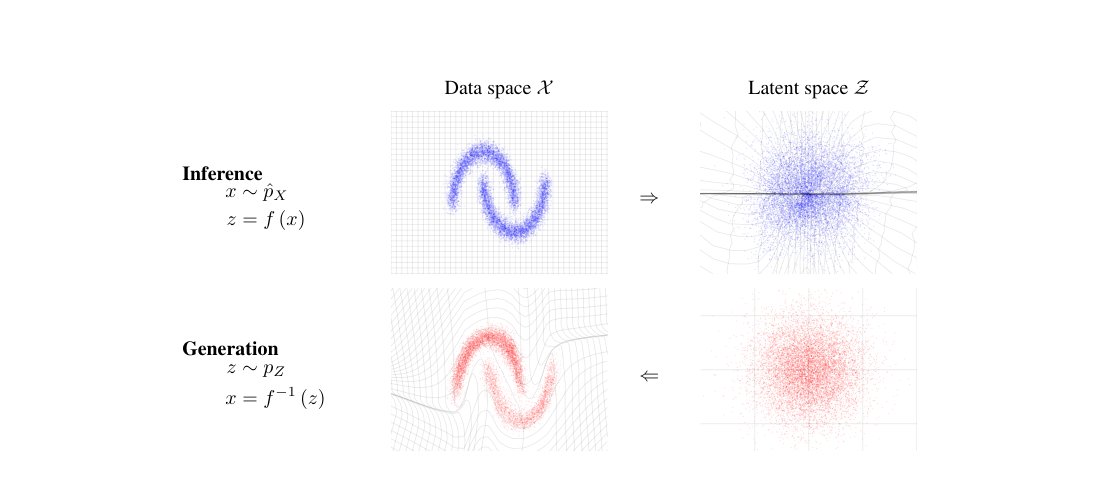
Figure 1: Real NVP learns an invertible, stable, mapping between a data distribution and a latent distribution (typically a Gaussian). Here we show a mapping that has been learned on a toy 2-d dataset. The function maps samples from the data distribution in the upper left into approximate samples from the latent distribution, in the upper right. This corresponds to exact inference of the latent state given the data. The inverse function, , maps samples from the latent distribution in the lower right into approximate samples from the data distribution in the lower left. This corresponds to exact generation of samples from the model. The transformation of grid lines in and space is additionally illustrated for both and .
| 数据空间 | 隐空间 | ||
|---|---|---|---|
| 推断 | |||
| 生成 |
图 1:Real NVP 学习数据分布 与隐分布 (通常是高斯)之间一个可逆且稳定的映射。这里展示的是在一个二维玩具数据集上学到的映射。函数 把左上角数据分布中的样本 映射成右上角隐分布中的近似样本 。这对应于给定数据时对隐状态的精确推断。逆函数 把右下角隐分布中的样本 映射成左下角数据分布中的近似样本 。这对应于从模型中精确生成样本。图中还分别展示了 与 对 和 空间中网格线的变换。
Substantial work on probabilistic generative models has focused on training models using maximum likelihood. One class of maximum likelihood models are those described by probabilistic undirected graphs, such as Restricted Boltzmann Machines [58] and Deep Boltzmann Machines [53]. These models are trained by taking advantage of the conditional independence property of their bipartite structure to allow efficient exact or approximate posterior inference on latent variables. However, because of the intractability of the associated marginal distribution over latent variables, their training, evaluation, and sampling procedures necessitate the use of approximations like Mean Field inference and Markov Chain Monte Carlo, whose convergence time for such complex models remains undetermined, often resulting in generation of highly correlated samples. Furthermore, these approximations can often hinder their performance [7].
大量关于概率生成模型的工作,聚焦于用极大似然来训练模型。一类极大似然模型由概率无向图描述,例如受限玻尔兹曼机(Restricted Boltzmann Machines)[58] 和深度玻尔兹曼机(Deep Boltzmann Machines)[53]。这些模型利用其二分结构的条件独立性,以便对隐变量做高效的精确或近似后验推断。不过,由于隐变量上的边缘分布不可处理,它们的训练、评估和采样过程必须借助平均场推断(Mean Field inference)和马尔可夫链蒙特卡洛(Markov Chain Monte Carlo)之类的近似;对这些复杂模型而言,这类近似的收敛时间仍不确定,往往会产生高度相关的样本。而且,这些近似还常常损害它们的表现[7]。
Directed graphical models are instead defined in terms of an ancestral sampling procedure, which is appealing both for its conceptual and computational simplicity. They lack, however, the conditional independence structure of undirected models, making exact and approximate posterior inference on latent variables cumbersome [56]. Recent advances in stochastic variational inference [27] and amortized inference [13, 43, 35, 49], allowed efficient approximate inference and learning of deep directed graphical models by maximizing a variational lower bound on the log-likelihood [45]. In particular, the variational autoencoder algorithm [35, 49] simultaneously learns a generative network, that maps gaussian latent variables to samples , and a matched approximate inference network that maps samples to a semantically meaningful latent representation , by exploiting the reparametrization trick [68]. Its success in leveraging recent advances in backpropagation [51, 39] in deep neural networks resulted in its adoption for several applications ranging from speech synthesis [12] to language modeling [8]. Still, the approximation in the inference process limits its ability to learn high dimensional deep representations, motivating recent work in improving approximate inference [42, 48, 55, 63, 10, 59, 34].
有向图模型则用祖先采样过程来定义,其概念上和计算上都简单,因而有吸引力。不过它们缺少无向模型那种条件独立结构,使得对隐变量做精确和近似后验推断都很麻烦[56]。随机变分推断[27]与摊销推断[13, 43, 35, 49]的近期进展,通过对数似然的变分下界做最大化[45],使深度有向图模型的近似推断和学习变得高效。特别是,变分自编码器算法[35, 49]利用重参数化技巧[68],同时学习一个把高斯隐变量 映射到样本 的生成网络,以及一个匹配的近似推断网络,把样本 映射到语义上有意义的隐表示 。它成功地借助深度神经网络中反向传播[51, 39]的近期进展,因而被用到从语音合成[12]到语言建模[8]的多种应用中。尽管如此,推断过程中的近似限制了它学习高维深度表示的能力,这也推动了改进近似推断的近期工作[42, 48, 55, 63, 10, 59, 34]。
Such approximations can be avoided altogether by abstaining from using latent variables. Auto-regressive models [18, 6, 37, 20] can implement this strategy while typically retaining a great deal of flexibility. This class of algorithms tractably models the joint distribution by decomposing it into a product of conditionals using the probability chain rule according to a fixed ordering over dimensions, simplifying log-likelihood evaluation and sampling. Recent work in this line of research has taken advantage of recent advances in recurrent networks [51], in particular long-short term memory [26], and residual networks [25, 24] in order to learn state-of-the-art generative image models [61, 46] and language models [32]. The ordering of the dimensions, although often arbitrary, can be critical to the training of the model [66]. The sequential nature of this model limits its computational efficiency. For example, its sampling procedure is sequential and non-parallelizable, which can become cumbersome in applications like speech and music synthesis, or real-time rendering.. Additionally, there is no natural latent representation associated with autoregressive models, and they have not yet been shown to be useful for semi-supervised learning.
如果完全不使用隐变量,就可以一并避开这类近似。自回归模型[18, 6, 37, 20]能够实现这一策略,同时通常仍保留很大的灵活性。这类算法按照维数上一个固定的次序,用概率链式法则把联合分布分解成条件分布的乘积,从而简化了对数似然评估和采样。这一方向的近期工作利用了循环网络[51]——尤其是长短期记忆[26]——以及残差网络[25, 24]的进展,以学习当时最先进的生成图像模型[61, 46]和语言模型[32]。维数的次序虽然往往是任意的,但对模型训练可能至关重要[66]。该模型的序贯本质限制了它的计算效率。例如,它的采样过程是串行且不可并行的,这在语音和音乐合成、或实时渲染等应用中会变得麻烦。此外,自回归模型没有与之对应的自然隐表示,也尚未被证明对半监督学习有用。
Generative Adversarial Networks (GANs) [21] on the other hand can train any differentiable generative network by avoiding the maximum likelihood principle altogether. Instead, the generative network is associated with a discriminator network whose task is to distinguish between samples and real data. Rather than using an intractable log-likelihood, this discriminator network provides the training signal in an adversarial fashion. Successfully trained GAN models [21, 15, 47] can consistently generate sharp and realistically looking samples [38]. However, metrics that measure the diversity in the generated samples are currently intractable [62, 22, 30]. Additionally, instability in their training process [47] requires careful hyperparameter tuning to avoid diverging behavior.
生成对抗网络(Generative Adversarial Networks,GANs)[21]则完全避开极大似然原则,就能训练任意可微的生成网络。生成网络与一个判别网络配对,后者的任务是区分样本和真实数据。这个判别网络不以不可处理的对数似然为信号,而是以对抗的方式提供训练信号。成功训练的 GAN 模型[21, 15, 47]能够稳定地生成锐利且看起来真实的样本[38]。不过,度量所生成样本多样性的指标目前仍不可处理[62, 22, 30]。此外,其训练过程中的不稳定性[47]需要仔细调节超参数,以避免发散。
Training such a generative network that maps latent variable to a sample does not in theory require a discriminator network as in GANs, or approximate inference as in variational autoencoders. Indeed, if is bijective, it can be trained through maximum likelihood using the change of variable formula:
训练这样一个把隐变量 映射到样本 的生成网络 ,理论上并不需要像 GAN 那样的判别网络,也不需要像变分自编码器那样的近似推断。事实上,如果 是双射,它就可以用变量替换公式通过极大似然来训练:
This formula has been discussed in several papers including the maximum likelihood formulation of independent components analysis (ICA) [4, 28], gaussianization [14, 11] and deep density models [5, 50, 17, 3]. As the existence proof of nonlinear ICA solutions [29] suggests, auto-regressive models can be seen as tractable instance of maximum likelihood nonlinear ICA, where the residual corresponds to the independent components. However, naive application of the change of variable formula produces models which are computationally expensive and poorly conditioned, and so large scale models of this type have not entered general use.
这一公式在若干论文中讨论过,包括独立成分分析(independent components analysis,ICA)的极大似然表述[4, 28]、高斯化(gaussianization)[14, 11]以及深度密度模型[5, 50, 17, 3]。正如非线性 ICA 解的存在性证明[29]所提示的,自回归模型可以看作可处理的极大似然非线性 ICA 实例,其中残差对应于独立成分。不过,朴素地应用变量替换公式会得到计算昂贵且条件很差的模型,因此这类大规模模型尚未进入普遍使用。
3 Model definition
3 模型定义
In this paper, we will tackle the problem of learning highly nonlinear models in high-dimensional continuous spaces through maximum likelihood. In order to optimize the log-likelihood, we introduce a more flexible class of architectures that enables the computation of log-likelihood on continuous data using the change of variable formula. Building on our previous work in [17], we define a powerful class of bijective functions which enable exact and tractable density evaluation and exact and tractable inference. Moreover, the resulting cost function does not to rely on a fixed form reconstruction cost such as square error [38, 47], and generates sharper samples as a result. Also, this flexibility helps us leverage recent advances in batch normalization [31] and residual networks [24, 25] to define a very deep multi-scale architecture with multiple levels of abstraction.
在本文中,我们将通过极大似然来处理在高维连续空间中学习高度非线性模型的问题。为了优化对数似然,我们引入一类更灵活的结构,能够用变量替换公式在连续数据上计算对数似然。在我们先前工作[17]的基础上,我们定义了一类强大的双射函数,使密度评估以及推断都能够精确且可处理。而且,由此得到的代价函数不必依赖固定形式的重建代价,例如平方误差[38, 47],因而能生成更锐利的样本。这种灵活性也帮助我们借助批归一化[31]和残差网络[24, 25]的近期进展,定义一个具有多个抽象层次的、非常深的多尺度结构。
3.1 Change of variable formula
3.1 变量替换公式
Given an observed data variable , a simple prior probability distribution on a latent variable , and a bijection (with ), the change of variable formula defines a model distribution on by
给定观测数据变量 、隐变量 上一个简单的先验概率分布 ,以及一个双射 (且 ),变量替换公式通过下式在 上定义一个模型分布
where is the Jacobian of at .
其中 是 在 处的雅可比矩阵。
Exact samples from the resulting distribution can be generated by using the inverse transform sampling rule [16]. A sample is drawn in the latent space, and its inverse image generates a sample in the original space. Computing the density on a point is accomplished by computing the density of its image and multiplying by the associated Jacobian determinant . See also Figure 1. Exact and efficient inference enables the accurate and fast evaluation of the model.
可以用逆变换采样规则[16]从所得分布中精确采样。先在隐空间中抽取一个样本 ,再取其原像 ,就在原始空间中生成一个样本。要计算某一点 上的密度,只需计算其像 的密度,再乘以相应的雅可比行列式 。亦可参见图 1。精确且高效的推断,使模型评估既准确又迅速。
3.2 Coupling layers
3.2 耦合层
(a) Forward propagation
(a)前向传播
Computing the Jacobian of functions with high-dimensional domain and codomain and computing the determinants of large matrices are in general computationally very expensive. This combined with the restriction to bijective functions makes Equation 2 appear impractical for modeling arbitrary distributions.
计算定义域和陪域都是高维的函数的雅可比矩阵,以及计算大型矩阵的行列式,一般来说在计算上都非常昂贵。这一点再加上必须限于双射函数,使公式 2 看起来并不适合用来建模任意分布。
As shown however in [17], by careful design of the function , a bijective model can be learned which is both tractable and extremely flexible. As computing the Jacobian determinant of the transformation is crucial to effectively train using this principle, this work exploits the simple observation that the determinant of a triangular matrix can be efficiently computed as the product of its diagonal terms.
不过,正如[17]所示,通过对函数 的精心设计,可以学到一个既可处理又极其灵活的双射模型。由于计算变换的雅可比行列式对有效地按这一原则训练至关重要,本工作利用一个简单观察:三角矩阵的行列式可以高效地算成其对角元的乘积。
We will build a flexible and tractable bijective function by stacking a sequence of simple bijections. In each simple bijection, part of the input vector is updated using a function which is simple to invert, but which depends on the remainder of the input vector in a complex way. We refer to each of these simple bijections as an affine coupling layer. Given a dimensional input and , the output of an affine coupling layer follows the equations
我们将通过堆叠一串简单双射,来构造一个灵活且可处理的双射函数。在每一个简单双射中,输入向量的一部分由一个易于求逆的函数来更新,但该函数又以复杂的方式依赖于输入向量的其余部分。我们把这些简单双射中的每一个称为一个仿射耦合层。给定 维输入 以及 ,仿射耦合层的输出 遵循下列方程
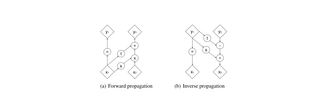
where and stand for scale and translation, and are functions from , and is the Hadamard product or element-wise product (see Figure 2(a)).
其中 和 分别表示缩放和平移,是从 到 的函数, 是 Hadamard 积或逐元素乘积(见图 2(a))。
3.3 Properties
3.3 性质
The Jacobian of this transformation is
这一变换的雅可比矩阵为
$$\displaystyle\frac{\partial y}{\partial x^{T}}=\left[\begin{array}[]{cc}{\mathbb{I}}{d}&0\
\frac{\partial y{d+1:D}}{\partial x_{1:d}^{T}}&\diag\big(\exp\left[s\left(x_{1:d}\right)\right]\big)\end{array}\right],$$
where is the diagonal matrix whose diagonal elements correspond to the vector . Given the observation that this Jacobian is triangular, we can efficiently compute its determinant as . Since computing the Jacobian determinant of the coupling layer operation does not involve computing the Jacobian of or , those functions can be arbitrarily complex. We will make them deep convolutional neural networks. Note that the hidden layers of and can have more features than their input and output layers.
其中 是对角元对应于向量 的对角矩阵。鉴于这一雅可比矩阵是三角的,我们可以高效地把它的行列式算成 。由于计算耦合层操作的雅可比行列式并不涉及计算 或 的雅可比矩阵,这些函数可以任意复杂。我们将让它们成为深度卷积神经网络。注意, 和 的隐层可以比它们的输入层和输出层拥有更多特征。
Another interesting property of these coupling layers in the context of defining probabilistic models is their invertibility. Indeed, computing the inverse is no more complex than the forward propagation (see Figure 2(b)),
在定义概率模型的语境中,这些耦合层的另一个有趣性质是它们的可逆性。事实上,计算逆并不比前向传播更复杂(见图 2(b)),
$$\displaystyle\begin{cases}y_{1:d}&=x_{1:d}\
y_{d+1:D}&=x_{d+1:D}\odot\exp\big(s(x_{1:d})\big)+t(x_{1:d})\end{cases} \ \displaystyle\Leftrightarrow\begin{cases}x_{1:d}&=y_{1:d}\
x_{d+1:D}&=\big(y_{d+1:D}-t(y_{1:d})\big)\odot\exp\big(-s(y_{1:d})\big),\end{cases} \tag{8}$$
meaning that sampling is as efficient as inference for this model. Note again that computing the inverse of the coupling layer does not require computing the inverse of or , so these functions can be arbitrarily complex and difficult to invert.
这意味着对该模型而言,采样与推断同样高效。再次注意,计算耦合层的逆并不要求计算 或 的逆,因此这些函数可以任意复杂、也难以求逆。
3.4 Masked convolution
3.4 掩码卷积
Partitioning can be implemented using a binary mask , and using the functional form for ,
划分可以用一个二值掩码 来实现,并采用如下关于 的函数形式,
We use two partitionings that exploit the local correlation structure of images: spatial checkerboard patterns, and channel-wise masking (see Figure 3). The spatial checkerboard pattern mask has value where the sum of spatial coordinates is odd, and otherwise. The channel-wise mask is for the first half of the channel dimensions and for the second half. For the models presented here, both and are rectified convolutional networks.
我们使用两种利用图像局部相关结构的划分:空间棋盘格模式,以及按通道的掩码(见图 3)。空间棋盘格模式掩码在空间坐标之和为奇数的位置取值为 ,否则为 。按通道的掩码 对通道维的前一半为 ,对后一半为 。对本文给出的模型, 和 都是带整流的卷积网络。

Figure 3: Masking schemes for affine coupling layers. On the left, a spatial checkerboard pattern mask. On the right, a channel-wise masking. The squeezing operation reduces the tensor (on the left) into a tensor (on the right). Before the squeezing operation, a checkerboard pattern is used for coupling layers while a channel-wise masking pattern is used afterward.
图 3:仿射耦合层的掩码方案。左侧是空间棋盘格模式掩码。右侧是按通道的掩码。挤压操作把(左侧的) 张量变成(右侧的) 张量。挤压操作之前,耦合层使用棋盘格模式;之后则使用按通道的掩码模式。
3.5 Combining coupling layers
3.5 组合耦合层
Although coupling layers can be powerful, their forward transformation leaves some components unchanged. This difficulty can be overcome by composing coupling layers in an alternating pattern, such that the components that are left unchanged in one coupling layer are updated in the next (see Figure 4(a)).
尽管耦合层可以很强大,它们的前向变换仍会使一部分分量保持不变。这一困难可以通过按交替模式组合耦合层来克服,使得在一个耦合层中保持不变的分量在下一个耦合层中被更新(见图 4(a))。
The Jacobian determinant of the resulting function remains tractable, relying on the fact that
所得函数的雅可比行列式仍然可处理,依据的是
Similarly, its inverse can be computed easily as
类似地,它的逆也很容易计算,因为
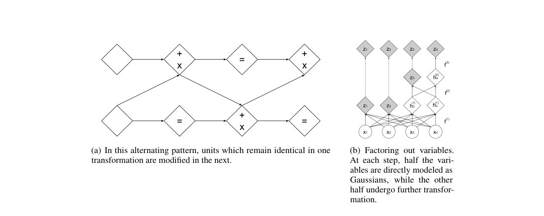
(a) In this alternating pattern, units which remain identical in one transformation are modified in the next.
(a)在这种交替模式中,某一次变换里保持不变的单元会在下一次变换中被修改。
3.6 Multi-scale architecture
3.6 多尺度结构
We implement a multi-scale architecture using a squeezing operation: for each channel, it divides the image into subsquares of shape , then reshapes them into subsquares of shape . The squeezing operation transforms an tensor into an tensor (see Figure 3), effectively trading spatial size for number of channels.
我们用一种挤压操作来实现多尺度结构:对每个通道,它把图像划分成形状为 的子方块,再把它们重排成形状为 的子方块。挤压操作把一个 张量变成一个 张量(见图 3),实际上是用空间尺寸去换通道数。
At each scale, we combine several operations into a sequence: we first apply three coupling layers with alternating checkerboard masks, then perform a squeezing operation, and finally apply three more coupling layers with alternating channel-wise masking. The channel-wise masking is chosen so that the resulting partitioning is not redundant with the previous checkerboard masking (see Figure 3). For the final scale, we only apply four coupling layers with alternating checkerboard masks.
在每个尺度上,我们把若干操作组合成一个序列:先用交替的棋盘格掩码施加三个耦合层,然后做一次挤压操作,最后再用交替的按通道掩码施加三个耦合层。按通道掩码的选择,使得所得划分不会与先前的棋盘格掩码冗余(见图 3)。对最后一个尺度,我们只施加四个带交替棋盘格掩码的耦合层。
Propagating a dimensional vector through all the coupling layers would be cumbersome, in terms of computational and memory cost, and in terms of the number of parameters that would need to be trained. For this reason we follow the design choice of [57] and factor out half of the dimensions at regular intervals (see Equation 15). We can define this operation recursively (see Figure 4(b)),
让一个 维向量穿过全部耦合层,在计算和内存代价上,以及在需要训练的参数数量上,都会很麻烦。因此我们沿用[57]的设计选择,每隔一段就把一半维度分解出去(见公式 15)。我们可以递归地定义这一操作(见图 4(b)),
In our experiments, we use this operation for . The sequence of coupling-squeezing-coupling operations described above is performed per layer when computing (Equation 15). At each layer, as the spatial resolution is reduced, the number of hidden layer features in and is doubled. All variables which have been factored out at different scales are concatenated to obtain the final transformed output (Equation 17).
在我们的实验中,对 使用这一操作。上面描述的耦合–挤压–耦合操作序列,在计算 时按层执行(公式 15)。在每一层,随着空间分辨率降低, 和 中隐层特征的数量加倍。在不同尺度上被分解出去的全部变量被拼接起来,得到最终的变换输出(公式 17)。
As a consequence, the model must Gaussianize units which are factored out at a finer scale (in an earlier layer) before those which are factored out at a coarser scale (in a later layer). This results in the definition of intermediary levels of representation [53, 49] corresponding to more local, fine-grained features as shown in Appendix D.
其结果是,模型必须先把在更细尺度(更早的层)分解出去的单元高斯化,再处理在更粗尺度(更晚的层)分解出去的单元。这就定义了对应于更局部、更细粒度特征的中间层表示[53, 49],如附录 D 所示。
Moreover, Gaussianizing and factoring out units in earlier layers has the practical benefit of distributing the loss function throughout the network, following the philosophy similar to guiding intermediate layers using intermediate classifiers [40]. It also reduces significantly the amount of computation and memory used by the model, allowing us to train larger models.
此外,在更早的层中把单元高斯化并分解出去,还有一个实际好处:把损失函数分布到整个网络中,其理念类似于用中间分类器去引导中间层[40]。它也显著减少了模型使用的计算量和内存,使我们能够训练更大的模型。
3.7 Batch normalization
3.7 批归一化
To further improve the propagation of training signal, we use deep residual networks [24, 25] with batch normalization [31] and weight normalization [2, 54] in and . As described in Appendix E we introduce and use a novel variant of batch normalization which is based on a running average over recent minibatches, and is thus more robust when training with very small minibatches.
为进一步改善训练信号的传播,我们在 和 中使用带批归一化[31]和权重归一化[2, 54]的深度残差网络[24, 25]。如附录 E 所述,我们引入并使用一种新的批归一化变体,它基于对近期小批量的滑动平均,因而在用非常小的小批量训练时更为稳健。
We also use apply batch normalization to the whole coupling layer output. The effects of batch normalization are easily included in the Jacobian computation, since it acts as a linear rescaling on each dimension. That is, given the estimated batch statistics and , the rescaling function
我们还对整个耦合层的输出施加批归一化。批归一化的效果很容易纳入雅可比计算,因为它在每个维度上相当于线性重标定。也就是说,给定估计的批次统计量 和 ,重标定函数
has a Jacobian determinant
其雅可比行列式为
This form of batch normalization can be seen as similar to reward normalization in deep reinforcement learning [44, 65].
这种形式的批归一化,可以看作类似于深度强化学习中的奖励归一化[44, 65]。
We found that the use of this technique not only allowed training with a deeper stack of coupling layers, but also alleviated the instability problem that practitioners often encounter when training conditional distributions with a scale parameter through a gradient-based approach.
我们发现,使用这一技术不仅允许用更深的耦合层堆叠来训练,还缓解了从业者在通过基于梯度的方法训练带尺度参数的条件分布时经常遇到的不稳定问题。
4 Experiments
4 实验
4.1 Procedure
4.1 步骤
The algorithm described in Equation 2 shows how to learn distributions on unbounded space. In general, the data of interest have bounded magnitude. For examples, the pixel values of an image typically lie in after application of the recommended jittering procedure [64, 62]. In order to reduce the impact of boundary effects, we instead model the density of , where is picked here as . We take into account this transformation when computing log-likelihood and bits per dimension. We also augment the CIFAR-10, CelebA and LSUN datasets during training to also include horizontal flips of the training examples.
公式 2 中描述的算法表明如何学习无界空间上的分布。一般而言,所关心的数据幅度是有界的。例如,在施加所建议的抖动步骤[64, 62]之后,图像的像素值通常落在 中。为了减轻边界效应的影响,我们改为建模 的密度,这里 取为 。在计算对数似然和每维比特数时,我们把这一变换考虑在内。我们还在训练期间对 CIFAR-10、CelebA 和 LSUN 数据集做增强,把训练样本的水平翻转也包括进去。
We train our model on four natural image datasets: CIFAR-10 [36], Imagenet [52], Large-scale Scene Understanding (LSUN) [70], CelebFaces Attributes (CelebA) [41]. More specifically, we train on the downsampled to and versions of Imagenet [46]. For the LSUN dataset, we train on the bedroom, tower and church outdoor categories. The procedure for LSUN is the same as in [47]: we downsample the image so that the smallest side is pixels and take random crops of . For CelebA, we use the same procedure as in [38]: we take an approximately central crop of then resize it to .
我们在四个自然图像数据集上训练模型:CIFAR-10[36]、Imagenet[52]、大规模场景理解(Large-scale Scene Understanding,LSUN)[70]、名人脸属性(CelebFaces Attributes,CelebA)[41]。更具体地说,我们在下采样到 和 的 Imagenet 版本上训练[46]。对 LSUN 数据集,我们在 bedroom、tower 和 church outdoor 类别上训练。LSUN 的处理步骤与[47]相同:把图像下采样到最短边为 像素,再取 的随机裁剪。对 CelebA,我们采用与[38]相同的步骤:取大约居中的 裁剪,再把它调整到 。
We use the multi-scale architecture described in Section 3.6 and use deep convolutional residual networks in the coupling layers with rectifier nonlinearity and skip-connections as suggested by [46]. To compute the scaling functions , we use a hyperbolic tangent function multiplied by a learned scale, whereas the translation function has an affine output. Our multi-scale architecture is repeated recursively until the input of the last recursion is a tensor. For datasets of images of size , we use residual blocks with hidden feature maps for the first coupling layers with checkerboard masking. Only residual blocks are used for images of size . We use a batch size of . For CIFAR-10, we use residual blocks, feature maps, and downscale only once. We optimize with ADAM [33] with default hyperparameters and use an regularization on the weight scale parameters with coefficient .
我们使用第 3.6 节描述的多尺度结构,并在耦合层中使用带整流非线性和跳跃连接的深度卷积残差网络,如[46]所建议。为了计算缩放函数 ,我们使用一个乘以可学习尺度的双曲正切函数,而平移函数 则采用仿射输出。我们的多尺度结构被递归地重复,直到最后一次递归的输入是一个 张量。对大小为 的图像数据集,我们在带棋盘格掩码的第一组耦合层中使用 个残差块、各有 张隐特征图。对大小为 的图像,只使用 个残差块。我们使用的 batch 大小为 。对 CIFAR-10,我们使用 个残差块、 张特征图,并且只下采样一次。我们用默认超参数的 ADAM[33] 来优化,并在权重尺度参数上使用系数为 的 正则化。
We set the prior to be an isotropic unit norm Gaussian. However, any distribution could be used for , including distributions that are also learned during training, such as from an auto-regressive model, or (with slight modifications to the training objective) a variational autoencoder.
我们把先验 设为各向同性的单位范数高斯。不过, 也可以使用任意分布,包括在训练期间一并学习的分布,例如来自自回归模型的分布,或(对训练目标稍作修改后)来自变分自编码器的分布。
4.2 Results
4.2 结果
| Dataset | PixelRNN [46] | Real NVP | Conv DRAW [22] | IAF-VAE [34] |
|---|---|---|---|---|
| CIFAR-10 | 3.00 | 3.49 | < 3.59 | < 3.28 |
| Imagenet () | 3.86 (3.83) | 4.28 (4.26) | < 4.40 (4.35) | |
| Imagenet () | 3.63 (3.57) | 3.98 (3.75) | < 4.10 (4.04) | |
| LSUN (bedroom) | 2.72 (2.70) | |||
| LSUN (tower) | 2.81 (2.78) | |||
| LSUN (church outdoor) | 3.08 (2.94) | |||
| CelebA | 3.02 (2.97) |
Table 1: Bits/dim results for CIFAR-10, Imagenet, LSUN datasets and CelebA. Test results for CIFAR-10 and validation results for Imagenet, LSUN and CelebA (with training results in parenthesis for reference).
| 数据集 | PixelRNN [46] | Real NVP | Conv DRAW [22] | IAF-VAE [34] |
|---|---|---|---|---|
| CIFAR-10 | 3.00 | 3.49 | < 3.59 | < 3.28 |
| Imagenet () | 3.86 (3.83) | 4.28 (4.26) | < 4.40 (4.35) | |
| Imagenet () | 3.63 (3.57) | 3.98 (3.75) | < 4.10 (4.04) | |
| LSUN (bedroom) | 2.72 (2.70) | |||
| LSUN (tower) | 2.81 (2.78) | |||
| LSUN (church outdoor) | 3.08 (2.94) | |||
| CelebA | 3.02 (2.97) |
表 1:CIFAR-10、Imagenet、LSUN 数据集和 CelebA 上的每维比特数结果。CIFAR-10 为测试结果,Imagenet、LSUN 和 CelebA 为验证结果(括号中给出训练结果供参考)。
We show in Table 1 that the number of bits per dimension, while not improving over the Pixel RNN [46] baseline, is competitive with other generative methods. As we notice that our performance increases with the number of parameters, larger models are likely to further improve performance. For CelebA and LSUN, the bits per dimension for the validation set was decreasing throughout training, so little overfitting is expected.
我们在表 1 中表明,每维比特数虽然没有超过 Pixel RNN[46] 这一基线,但与其他生成方法相比仍具有竞争力。由于我们注意到性能会随参数数量增加而提高,更大的模型很可能会进一步改善表现。对 CelebA 和 LSUN,验证集上的每维比特数在整个训练过程中都在下降,因此预期过拟合很少。
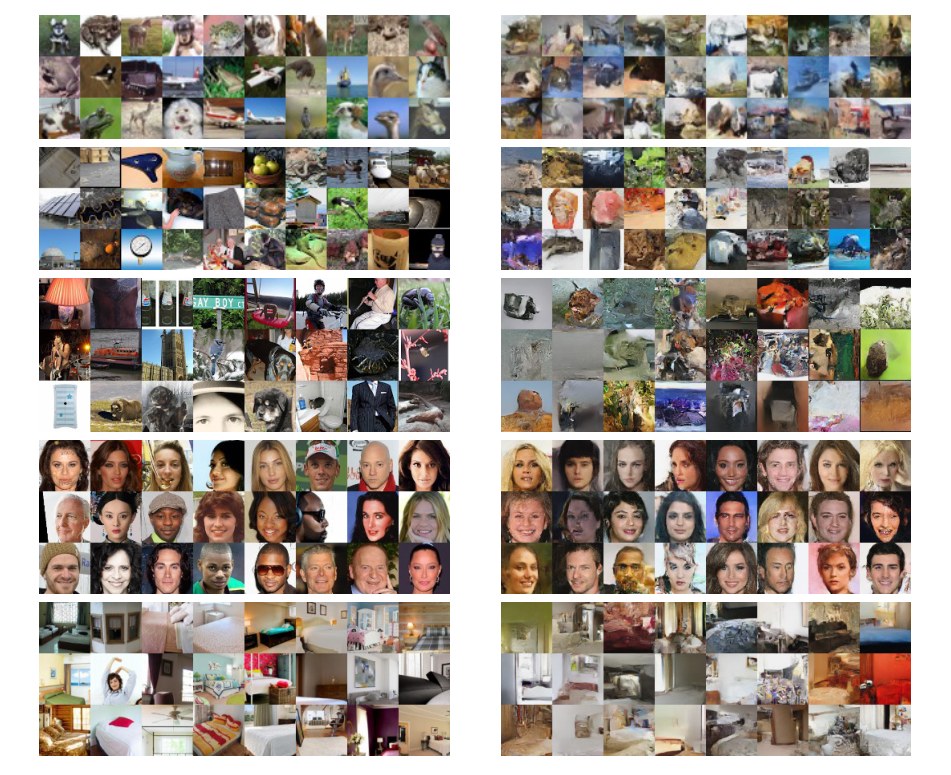
Figure 5: On the left column, examples from the dataset. On the right column, samples from the model trained on the dataset. The datasets shown in this figure are in order: CIFAR-10, Imagenet (), Imagenet (), CelebA, LSUN (bedroom).
图 5:左列为数据集中的示例。右列为在该数据集上训练的模型所生成的样本。本图所示数据集依次为:CIFAR-10、Imagenet()、Imagenet()、CelebA、LSUN(bedroom)。
We show in Figure 5 samples generated from the model with training examples from the dataset for comparison. As mentioned in [62, 22], maximum likelihood is a principle that values diversity over sample quality in a limited capacity setting. As a result, our model outputs sometimes highly improbable samples as we can notice especially on CelebA. As opposed to variational autoencoders, the samples generated from our model look not only globally coherent but also sharp. Our hypothesis is that as opposed to these models, real NVP does not rely on fixed form reconstruction cost like an norm which tends to reward capturing low frequency components more heavily than high frequency components. Unlike autoregressive models, sampling from our model is done very efficiently as it is parallelized over input dimensions. On Imagenet and LSUN, our model seems to have captured well the notion of background/foreground and lighting interactions such as luminosity and consistent light source direction for reflectance and shadows.
我们在图 5 中展示从模型生成的样本,并附上数据集中的训练示例以供比较。正如[62, 22]所提到的,在容量有限的设定下,极大似然是一种相对样本质量更看重多样性的原则。因此,我们的模型有时会输出极不可能的样本,这一点在 CelebA 上尤其可以注意到。与变分自编码器不同,从我们模型生成的样本不仅整体上连贯,而且锐利。我们的假设是:与这些模型不同,real NVP 并不依赖像 范数这样的固定形式重建代价——这类代价往往更重地奖励捕捉低频分量,而不是高频分量。与自回归模型不同,从我们的模型采样非常高效,因为它在输入维上是并行的。在 Imagenet 和 LSUN 上,我们的模型似乎很好地抓住了前景/背景的概念,以及诸如亮度、反射和阴影中一致的光源方向这类光照相互作用。
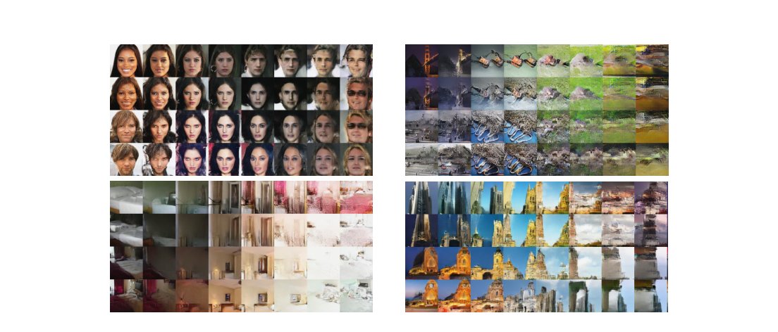
Figure 6: Manifold generated from four examples in the dataset. Clockwise from top left: CelebA, Imagenet (), LSUN (tower), LSUN (bedroom).
图 6:由数据集中四个示例生成的流形。从左上起顺时针依次为:CelebA、Imagenet()、LSUN(tower)、LSUN(bedroom)。
We also illustrate the smooth semantically consistent meaning of our latent variables. In the latent space, we define a manifold based on four validation examples , , , , and parametrized by two parameters and by,
我们还展示了隐变量平滑且语义一致的含义。在隐空间中,我们基于四个验证示例 、、、,并用两个参数 和 来参数化一个流形,
We project the resulting manifold back into the data space by computing . Results are shown Figure 6. We observe that the model seems to have organized the latent space with a notion of meaning that goes well beyond pixel space interpolation. More visualization are shown in the Appendix. To further test whether the latent space has a consistent semantic interpretation, we trained a class-conditional model on CelebA, and found that the learned representation had a consistent semantic meaning across class labels (see Appendix F).
我们通过计算 ,把所得流形投影回数据空间。结果见图 6。我们观察到,模型似乎已经按一种远超出像素空间插值的含义组织了隐空间。更多可视化见附录。为进一步检验隐空间是否具有一致的语义解释,我们在 CelebA 上训练了一个类别条件模型,并发现学到的表示在不同类别标签之间具有一致的语义含义(见附录 F)。
5 Discussion and conclusion
5 讨论与结论
In this paper, we have defined a class of invertible functions with tractable Jacobian determinant, enabling exact and tractable log-likelihood evaluation, inference, and sampling. We have shown that this class of generative model achieves competitive performances, both in terms of sample quality and log-likelihood. Many avenues exist to further improve the functional form of the transformations, for instance by exploiting the latest advances in dilated convolutions [69] and residual networks architectures [60].
在本文中,我们定义了一类雅可比行列式可处理的可逆函数,从而能够精确且可处理地做对数似然评估、推断和采样。我们表明,这类生成模型在样本质量和对数似然两方面都达到了有竞争力的表现。进一步改进这些变换的函数形式还有许多途径,例如利用膨胀卷积[69]和残差网络结构[60]的最新进展。
This paper presented a technique bridging the gap between auto-regressive models, variational autoencoders, and generative adversarial networks. Like auto-regressive models, it allows tractable and exact log-likelihood evaluation for training. It allows however a much more flexible functional form, similar to that in the generative model of variational autoencoders. This allows for fast and exact sampling from the model distribution. Like GANs, and unlike variational autoencoders, our technique does not require the use of a fixed form reconstruction cost, and instead defines a cost in terms of higher level features, generating sharper images. Finally, unlike both variational autoencoders and GANs, our technique is able to learn a semantically meaningful latent space which is as high dimensional as the input space. This may make the algorithm particularly well suited to semi-supervised learning tasks, as we hope to explore in future work.
本文提出的技术弥合了自回归模型、变分自编码器和生成对抗网络之间的差距。像自回归模型一样,它允许用可处理且精确的对数似然评估来训练。但它允许远为灵活的函数形式,类似于变分自编码器中的生成模型。这使得可以从模型分布中快速且精确地采样。像 GAN 一样,而不像变分自编码器,我们的技术不需要使用固定形式的重建代价,而是用更高层特征来定义代价,从而生成更锐利的图像。最后,与变分自编码器和 GAN 都不同,我们的技术能够学习一个语义上有意义、且维数与输入空间一样高的隐空间。这可能使该算法特别适合半监督学习任务,我们希望在未来工作中加以探索。
Real NVP generative models can additionally be conditioned on additional variables (for instance class labels) to create a structured output algorithm. More so, as the resulting class of invertible transformations can be treated as a probability distribution in a modular way, it can also be used to improve upon other probabilistic models like auto-regressive models and variational autoencoders. For variational autoencoders, these transformations could be used both to enable a more flexible reconstruction cost [38] and a more flexible stochastic inference distribution [48]. Probabilistic models in general can also benefit from batch normalization techniques as applied in this paper.
Real NVP 生成模型还可以条件于额外变量(例如类别标签),以形成一个结构化输出算法。更进一步,由于所得的这类可逆变换可以模块化地当作一个概率分布来处理,它也可以用来改进其他概率模型,例如自回归模型和变分自编码器。对变分自编码器而言,这些变换既可以用来实现更灵活的重建代价[38],也可以用来实现更灵活的随机推断分布[48]。一般的概率模型也可以受益于本文所采用的批归一化技术。
The definition of powerful and trainable invertible functions can also benefit domains other than generative unsupervised learning. For example, in reinforcement learning, these invertible functions can help extend the set of functions for which an operation is tractable for continuous Q-learning [23] or find representation where local linear Gaussian approximations are more appropriate [67].
强大且可训练的可逆函数的定义,也可以使生成式无监督学习以外的领域受益。例如,在强化学习中,这些可逆函数可以帮助扩展那些对连续 Q 学习[23]而言 操作可处理的函数集合,或找到局部线性高斯近似更为合适的表示[67]。
6 Acknowledgments
6 致谢
The authors thank the developers of Tensorflow [1]. We thank Sherry Moore, David Andersen and Jon Shlens for their help in implementing the model. We thank Aäron van den Oord, Yann Dauphin, Kyle Kastner, Chelsea Finn, Maithra Raghu, David Warde-Farley, Daniel Jiwoong Im and Oriol Vinyals for fruitful discussions. Finally, we thank Ben Poole, Rafal Jozefowicz and George Dahl for their input on a draft of the paper.
作者感谢 Tensorflow[1] 的开发者。我们感谢 Sherry Moore、David Andersen 和 Jon Shlens 在实现模型上的帮助。我们感谢 Aäron van den Oord、Yann Dauphin、Kyle Kastner、Chelsea Finn、Maithra Raghu、David Warde-Farley、Daniel Jiwoong Im 和 Oriol Vinyals 富有成效的讨论。最后,我们感谢 Ben Poole、Rafal Jozefowicz 和 George Dahl 对论文草稿提出的意见。
References
参考文献
[1] Martın Abadi, Ashish Agarwal, Paul Barham, Eugene Brevdo, Zhifeng Chen, Craig Citro, Greg S Corrado, Andy Davis, Jeffrey Dean, Matthieu Devin, et al. Tensorflow: Large-scale machine learning on heterogeneous distributed systems. arXiv preprint arXiv:1603.04467 , 2016.
[2] Vijay Badrinarayanan, Bamdev Mishra, and Roberto Cipolla. Understanding symmetries in deep networks. arXiv preprint arXiv:1511.01029 , 2015.
[3] Johannes Ballé, Valero Laparra, and Eero P Simoncelli. Density modeling of images using a generalized normalization transformation. arXiv preprint arXiv:1511.06281 , 2015.
[4] Anthony J Bell and Terrence J Sejnowski. An information-maximization approach to blind separation and blind deconvolution. Neural computation , 7(6):1129–1159, 1995.
[5] Yoshua Bengio. Artificial neural networks and their application to sequence recognition. 1991.
[6] Yoshua Bengio and Samy Bengio. Modeling high-dimensional discrete data with multi-layer neural networks. In NIPS , volume 99, pages 400–406, 1999.
[7] Mathias Berglund and Tapani Raiko. Stochastic gradient estimate variance in contrastive divergence and persistent contrastive divergence. arXiv preprint arXiv:1312.6002 , 2013.
[8] Samuel R Bowman, Luke Vilnis, Oriol Vinyals, Andrew M Dai, Rafal Jozefowicz, and Samy Bengio. Generating sentences from a continuous space. arXiv preprint arXiv:1511.06349 , 2015.
[9] Joan Bruna, Pablo Sprechmann, and Yann LeCun. Super-resolution with deep convolutional sufficient statistics. arXiv preprint arXiv:1511.05666 , 2015.
[10] Yuri Burda, Roger Grosse, and Ruslan Salakhutdinov. Importance weighted autoencoders. arXiv preprint arXiv:1509.00519 , 2015.
[11] Scott Shaobing Chen and Ramesh A Gopinath. Gaussianization. In Advances in Neural Information Processing Systems , 2000.
[12] Junyoung Chung, Kyle Kastner, Laurent Dinh, Kratarth Goel, Aaron C Courville, and Yoshua Bengio. A recurrent latent variable model for sequential data. In Advances in neural information processing systems , pages 2962–2970, 2015.
[13] Peter Dayan, Geoffrey E Hinton, Radford M Neal, and Richard S Zemel. The helmholtz machine. Neural computation , 7(5):889–904, 1995.
[14] Gustavo Deco and Wilfried Brauer. Higher order statistical decorrelation without information loss. In G. Tesauro, D. S. Touretzky, and T. K. Leen, editors, Advances in Neural Information Processing Systems 7 , pages 247–254. MIT Press, 1995.
[15] Emily L. Denton, Soumith Chintala, Arthur Szlam, and Rob Fergus. Deep generative image models using a laplacian pyramid of adversarial networks. In Advances in Neural Information Processing Systems 28: Annual Conference on Neural Information Processing Systems 2015, December 7-12, 2015, Montreal, Quebec, Canada , pages 1486–1494, 2015.
[16] Luc Devroye. Sample-based non-uniform random variate generation. In Proceedings of the 18th conference on Winter simulation , pages 260–265. ACM, 1986.
[17] Laurent Dinh, David Krueger, and Yoshua Bengio. Nice: non-linear independent components estimation. arXiv preprint arXiv:1410.8516 , 2014.
[18] Brendan J Frey. Graphical models for machine learning and digital communication . MIT press, 1998.
[19] Leon A. Gatys, Alexander S. Ecker, and Matthias Bethge. Texture synthesis using convolutional neural networks. In Advances in Neural Information Processing Systems 28: Annual Conference on Neural Information Processing Systems 2015, December 7-12, 2015, Montreal, Quebec, Canada , pages 262–270, 2015.
[20] Mathieu Germain, Karol Gregor, Iain Murray, and Hugo Larochelle. MADE: masked autoencoder for distribution estimation. CoRR , abs/1502.03509, 2015.
[21] Ian J. Goodfellow, Jean Pouget-Abadie, Mehdi Mirza, Bing Xu, David Warde-Farley, Sherjil Ozair, Aaron C. Courville, and Yoshua Bengio. Generative adversarial nets. In Advances in Neural Information Processing Systems 27: Annual Conference on Neural Information Processing Systems 2014, December 8-13 2014, Montreal, Quebec, Canada , pages 2672–2680, 2014.
[22] Karol Gregor, Frederic Besse, Danilo Jimenez Rezende, Ivo Danihelka, and Daan Wierstra. Towards conceptual compression. arXiv preprint arXiv:1604.08772 , 2016.
[23] Shixiang Gu, Timothy Lillicrap, Ilya Sutskever, and Sergey Levine. Continuous deep q-learning with model-based acceleration. arXiv preprint arXiv:1603.00748 , 2016.
[24] Kaiming He, Xiangyu Zhang, Shaoqing Ren, and Jian Sun. Deep residual learning for image recognition. CoRR , abs/1512.03385, 2015.
[25] Kaiming He, Xiangyu Zhang, Shaoqing Ren, and Jian Sun. Identity mappings in deep residual networks. CoRR , abs/1603.05027, 2016.
[26] Sepp Hochreiter and Jürgen Schmidhuber. Long short-term memory. Neural Computation , 9(8):1735–1780, 1997.
[27] Matthew D Hoffman, David M Blei, Chong Wang, and John Paisley. Stochastic variational inference. The Journal of Machine Learning Research , 14(1):1303–1347, 2013.
[28] Aapo Hyvärinen, Juha Karhunen, and Erkki Oja. Independent component analysis , volume 46. John Wiley & Sons, 2004.
[29] Aapo Hyvärinen and Petteri Pajunen. Nonlinear independent component analysis: Existence and uniqueness results. Neural Networks , 12(3):429–439, 1999.
[30] Daniel Jiwoong Im, Chris Dongjoo Kim, Hui Jiang, and Roland Memisevic. Generating images with recurrent adversarial networks. arXiv preprint arXiv:1602.05110 , 2016.
[31] Sergey Ioffe and Christian Szegedy. Batch normalization: Accelerating deep network training by reducing internal covariate shift. arXiv preprint arXiv:1502.03167 , 2015.
[32] Rafal Józefowicz, Oriol Vinyals, Mike Schuster, Noam Shazeer, and Yonghui Wu. Exploring the limits of language modeling. CoRR , abs/1602.02410, 2016.
[33] Diederik Kingma and Jimmy Ba. Adam: A method for stochastic optimization. arXiv preprint arXiv:1412.6980 , 2014.
[34] Diederik P Kingma, Tim Salimans, and Max Welling. Improving variational inference with inverse autoregressive flow. arXiv preprint arXiv:1606.04934 , 2016.
[35] Diederik P Kingma and Max Welling. Auto-encoding variational bayes. arXiv preprint arXiv:1312.6114 , 2013.
[36] Alex Krizhevsky and Geoffrey Hinton. Learning multiple layers of features from tiny images, 2009.
[37] Hugo Larochelle and Iain Murray. The neural autoregressive distribution estimator. In AISTATS , 2011.
[38] Anders Boesen Lindbo Larsen, Søren Kaae Sønderby, and Ole Winther. Autoencoding beyond pixels using a learned similarity metric. CoRR , abs/1512.09300, 2015.
[39] Yann A LeCun, Léon Bottou, Genevieve B Orr, and Klaus-Robert Müller. Efficient backprop. In Neural networks: Tricks of the trade , pages 9–48. Springer, 2012.
[40] Chen-Yu Lee, Saining Xie, Patrick Gallagher, Zhengyou Zhang, and Zhuowen Tu. Deeply-supervised nets. arXiv preprint arXiv:1409.5185 , 2014.
[41] Ziwei Liu, Ping Luo, Xiaogang Wang, and Xiaoou Tang. Deep learning face attributes in the wild. In Proceedings of International Conference on Computer Vision (ICCV) , December 2015.
[42] Lars Maaløe, Casper Kaae Sønderby, Søren Kaae Sønderby, and Ole Winther. Auxiliary deep generative models. arXiv preprint arXiv:1602.05473 , 2016.
[43] Andriy Mnih and Karol Gregor. Neural variational inference and learning in belief networks. arXiv preprint arXiv:1402.0030 , 2014.
[44] Volodymyr Mnih, Koray Kavukcuoglu, David Silver, Andrei A Rusu, Joel Veness, Marc G Bellemare, Alex Graves, Martin Riedmiller, Andreas K Fidjeland, Georg Ostrovski, et al. Human-level control through deep reinforcement learning. Nature , 518(7540):529–533, 2015.
[45] Radford M Neal and Geoffrey E Hinton. A view of the em algorithm that justifies incremental, sparse, and other variants. In Learning in graphical models , pages 355–368. Springer, 1998.
[46] Aaron van den Oord, Nal Kalchbrenner, and Koray Kavukcuoglu. Pixel recurrent neural networks. arXiv preprint arXiv:1601.06759 , 2016.
[47] Alec Radford, Luke Metz, and Soumith Chintala. Unsupervised representation learning with deep convolutional generative adversarial networks. CoRR , abs/1511.06434, 2015.
[48] Danilo Jimenez Rezende and Shakir Mohamed. Variational inference with normalizing flows. arXiv preprint arXiv:1505.05770 , 2015.
[49] Danilo Jimenez Rezende, Shakir Mohamed, and Daan Wierstra. Stochastic backpropagation and approximate inference in deep generative models. arXiv preprint arXiv:1401.4082 , 2014.
[50] Oren Rippel and Ryan Prescott Adams. High-dimensional probability estimation with deep density models. arXiv preprint arXiv:1302.5125 , 2013.
[51] David E Rumelhart, Geoffrey E Hinton, and Ronald J Williams. Learning representations by back-propagating errors. Cognitive modeling , 5(3):1, 1988.
[52] Olga Russakovsky, Jia Deng, Hao Su, Jonathan Krause, Sanjeev Satheesh, Sean Ma, Zhiheng Huang, Andrej Karpathy, Aditya Khosla, Michael Bernstein, et al. Imagenet large scale visual recognition challenge. International Journal of Computer Vision , 115(3):211–252, 2015.
[53] Ruslan Salakhutdinov and Geoffrey E Hinton. Deep boltzmann machines. In International conference on artificial intelligence and statistics , pages 448–455, 2009.
[54] Tim Salimans and Diederik P Kingma. Weight normalization: A simple reparameterization to accelerate training of deep neural networks. arXiv preprint arXiv:1602.07868 , 2016.
[55] Tim Salimans, Diederik P Kingma, and Max Welling. Markov chain monte carlo and variational inference: Bridging the gap. arXiv preprint arXiv:1410.6460 , 2014.
[56] Lawrence K Saul, Tommi Jaakkola, and Michael I Jordan. Mean field theory for sigmoid belief networks. Journal of artificial intelligence research , 4(1):61–76, 1996.
[57] Karen Simonyan and Andrew Zisserman. Very deep convolutional networks for large-scale image recognition. arXiv preprint arXiv:1409.1556 , 2014.
[58] Paul Smolensky. Information processing in dynamical systems: Foundations of harmony theory. Technical report, DTIC Document, 1986.
[59] Jascha Sohl-Dickstein, Eric A. Weiss, Niru Maheswaranathan, and Surya Ganguli. Deep unsupervised learning using nonequilibrium thermodynamics. In Proceedings of the 32nd International Conference on Machine Learning, ICML 2015, Lille, France, 6-11 July 2015 , pages 2256–2265, 2015.
[60] Sasha Targ, Diogo Almeida, and Kevin Lyman. Resnet in resnet: Generalizing residual architectures. CoRR , abs/1603.08029, 2016.
[61] Lucas Theis and Matthias Bethge. Generative image modeling using spatial lstms. In Advances in Neural Information Processing Systems , pages 1918–1926, 2015.
[62] Lucas Theis, Aäron Van Den Oord, and Matthias Bethge. A note on the evaluation of generative models. CoRR , abs/1511.01844, 2015.
[63] Dustin Tran, Rajesh Ranganath, and David M Blei. Variational gaussian process. arXiv preprint arXiv:1511.06499 , 2015.
[64] Benigno Uria, Iain Murray, and Hugo Larochelle. Rnade: The real-valued neural autoregressive density-estimator. In Advances in Neural Information Processing Systems , pages 2175–2183, 2013.
[65] Hado van Hasselt, Arthur Guez, Matteo Hessel, and David Silver. Learning functions across many orders of magnitudes. arXiv preprint arXiv:1602.07714 , 2016.
[66] Oriol Vinyals, Samy Bengio, and Manjunath Kudlur. Order matters: Sequence to sequence for sets. arXiv preprint arXiv:1511.06391 , 2015.
[67] Manuel Watter, Jost Springenberg, Joschka Boedecker, and Martin Riedmiller. Embed to control: A locally linear latent dynamics model for control from raw images. In Advances in Neural Information Processing Systems , pages 2728–2736, 2015.
[68] Ronald J Williams. Simple statistical gradient-following algorithms for connectionist reinforcement learning. Machine learning , 8(3-4):229–256, 1992.
[69] Fisher Yu and Vladlen Koltun. Multi-scale context aggregation by dilated convolutions. arXiv preprint arXiv:1511.07122 , 2015.
[70] Fisher Yu, Yinda Zhang, Shuran Song, Ari Seff, and Jianxiong Xiao. Construction of a large-scale image dataset using deep learning with humans in the loop. arXiv preprint arXiv:1506.03365 , 2015.
[71] Richard Zhang, Phillip Isola, and Alexei A Efros. Colorful image colorization. arXiv preprint arXiv:1603.08511 , 2016.
Appendix A Samples
附录 A 样本
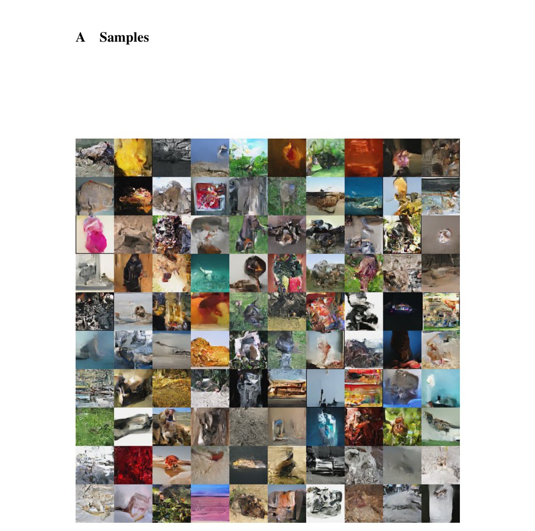
Figure 7: Samples from a model trained on Imagenet ().
图 7:在 Imagenet()上训练的模型所生成的样本。
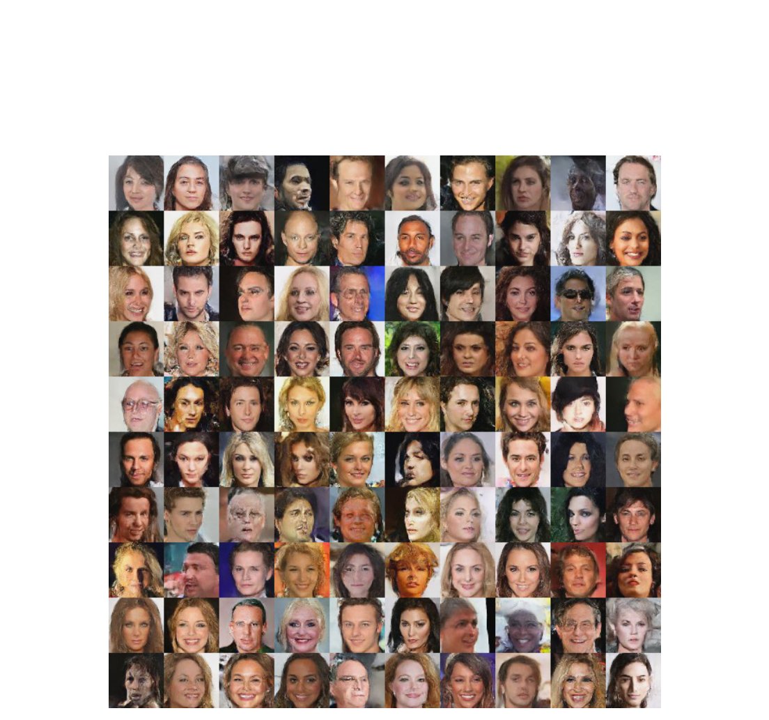
Figure 8: Samples from a model trained on CelebA.
图 8:在 CelebA 上训练的模型所生成的样本。
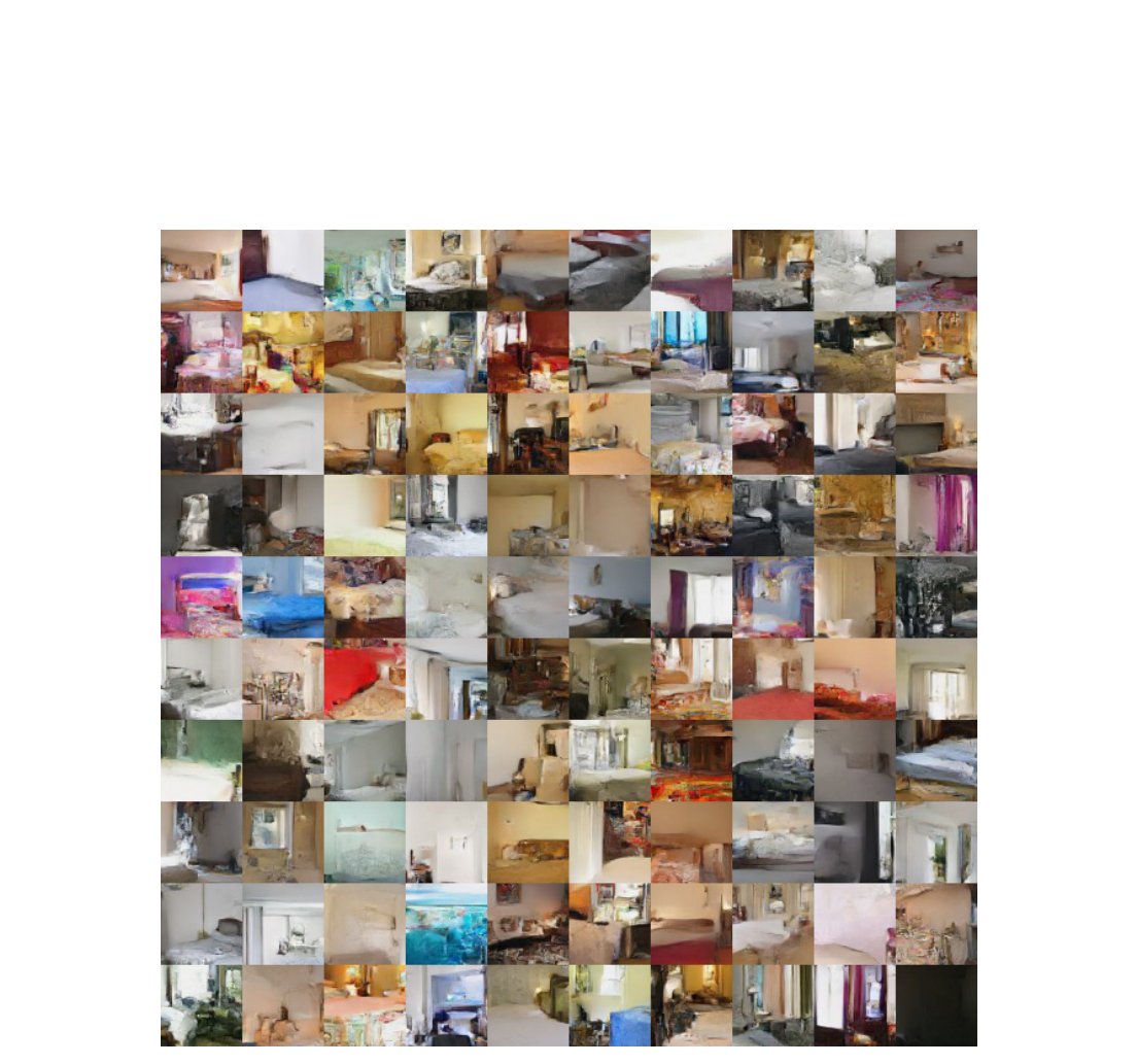
Figure 9: Samples from a model trained on LSUN (bedroom category).
图 9:在 LSUN(bedroom 类别)上训练的模型所生成的样本。
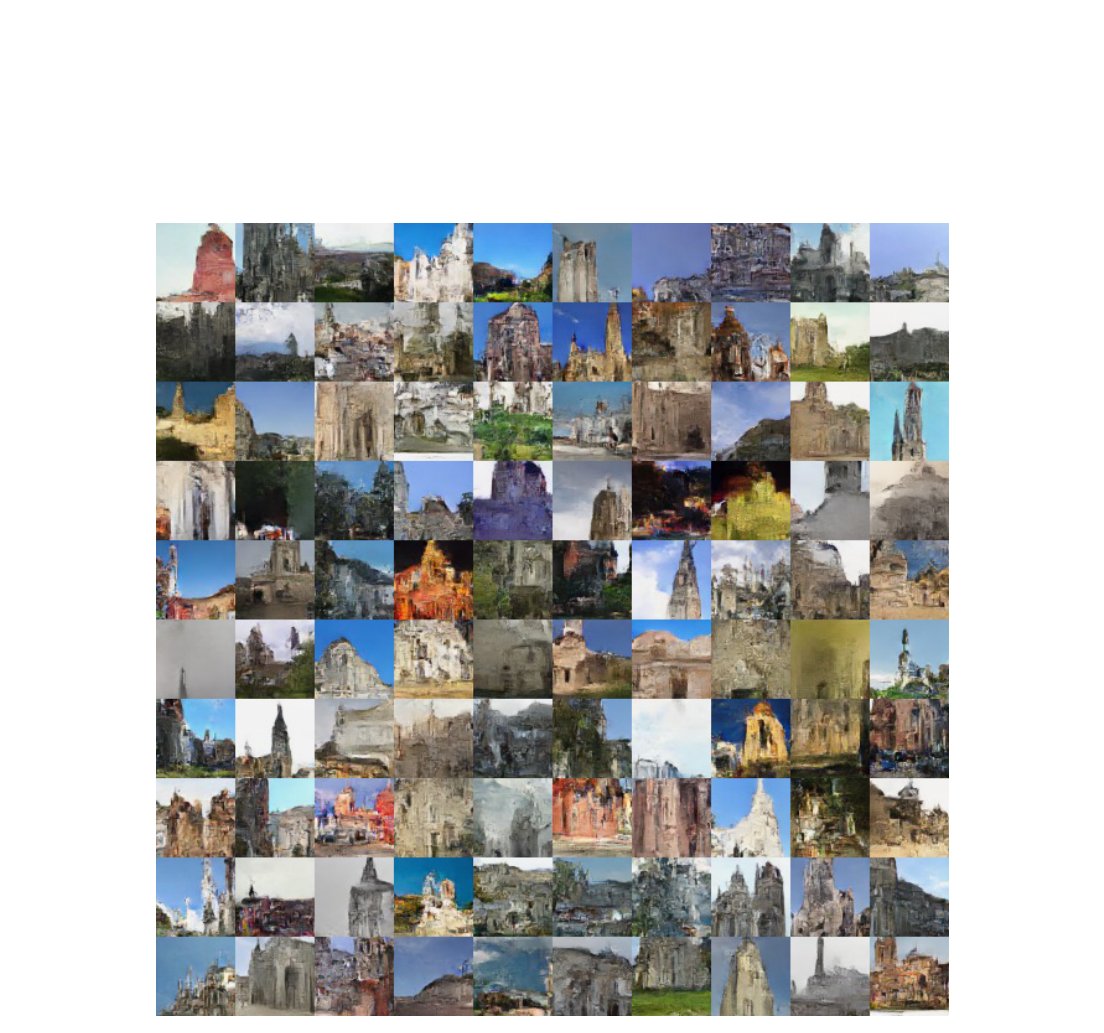
Figure 10: Samples from a model trained on LSUN (church outdoor category).
图 10:在 LSUN(church outdoor 类别)上训练的模型所生成的样本。
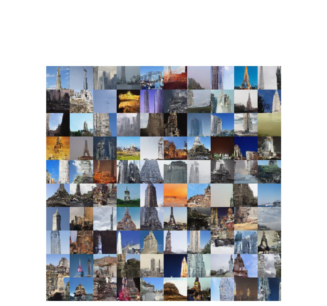
Figure 11: Samples from a model trained on LSUN (tower category).
图 11:在 LSUN(tower 类别)上训练的模型所生成的样本。
Appendix B Manifold
附录 B 流形
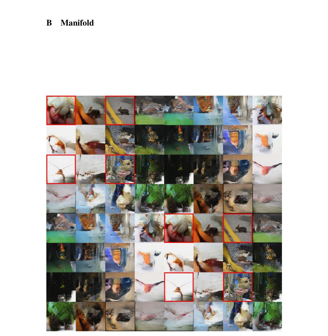
Figure 12: Manifold from a model trained on Imagenet (). Images with red borders are taken from the validation set, and define the manifold. The manifold was computed as described in Equation 20, where the x-axis corresponds to , and the y-axis to , and where .
图 12:在 Imagenet()上训练的模型得到的流形。带红色边框的图像取自验证集,并用来定义该流形。流形按公式 20 计算,其中 x 轴对应于 ,y 轴对应于 ,且 。
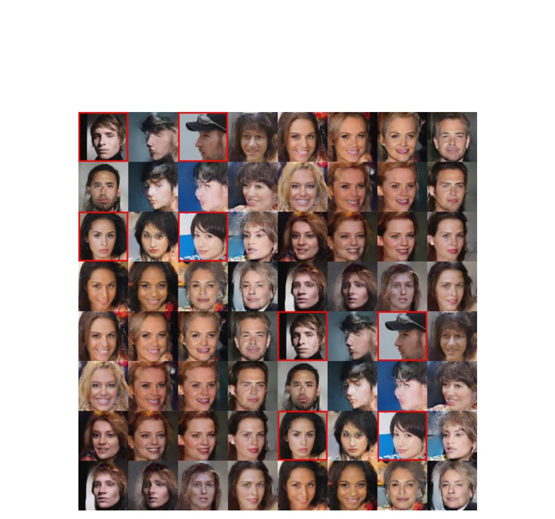
Figure 13: Manifold from a model trained on CelebA. Images with red borders are taken from the training set, and define the manifold. The manifold was computed as described in Equation 20, where the x-axis corresponds to , and the y-axis to , and where .
图 13:在 CelebA 上训练的模型得到的流形。带红色边框的图像取自训练集,并用来定义该流形。流形按公式 20 计算,其中 x 轴对应于 ,y 轴对应于 ,且 。
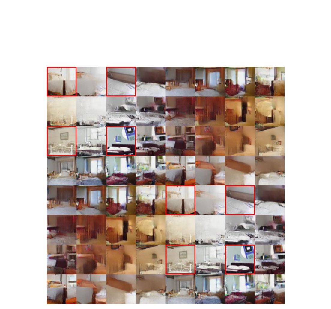
Figure 14: Manifold from a model trained on LSUN (bedroom category). Images with red borders are taken from the validation set, and define the manifold. The manifold was computed as described in Equation 20, where the x-axis corresponds to , and the y-axis to , and where .
图 14:在 LSUN(bedroom 类别)上训练的模型得到的流形。带红色边框的图像取自验证集,并用来定义该流形。流形按公式 20 计算,其中 x 轴对应于 ,y 轴对应于 ,且 。
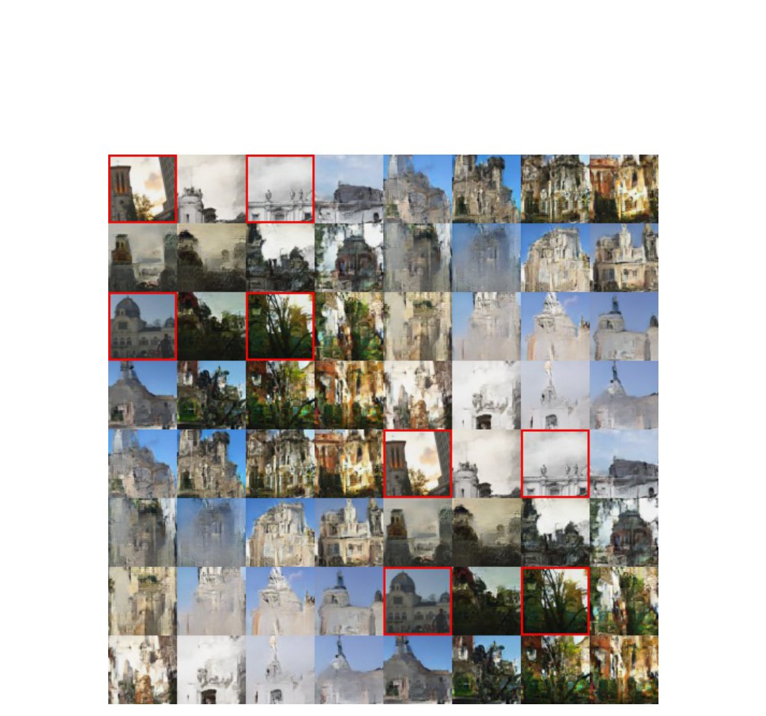
Figure 15: Manifold from a model trained on LSUN (church outdoor category). Images with red borders are taken from the validation set, and define the manifold. The manifold was computed as described in Equation 20, where the x-axis corresponds to , and the y-axis to , and where .
图 15:在 LSUN(church outdoor 类别)上训练的模型得到的流形。带红色边框的图像取自验证集,并用来定义该流形。流形按公式 20 计算,其中 x 轴对应于 ,y 轴对应于 ,且 。
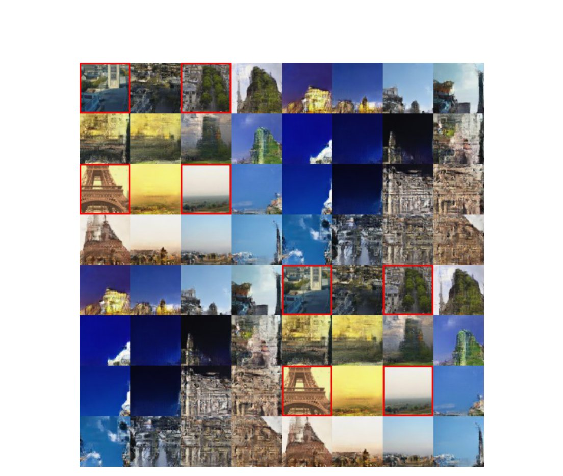
Figure 16: Manifold from a model trained on LSUN (tower category). Images with red borders are taken from the validation set, and define the manifold. The manifold was computed as described in Equation 20, where the x-axis corresponds to , and the y-axis to , and where .
图 16:在 LSUN(tower 类别)上训练的模型得到的流形。带红色边框的图像取自验证集,并用来定义该流形。流形按公式 20 计算,其中 x 轴对应于 ,y 轴对应于 ,且 。
Appendix C Extrapolation
附录 C 外推
Inspired by the texture generation work by [19, 61] and extrapolation test with DCGAN [47], we also evaluate the statistics captured by our model by generating images twice or ten times as large as present in the dataset. As we can observe in the following figures, our model seems to successfully create a “texture” representation of the dataset while maintaining a spatial smoothness through the image. Our convolutional architecture is only aware of the position of considered pixel through edge effects in convolutions, therefore our model is similar to a stationary process. This also explains why these samples are more consistent in LSUN, where the training data was obtained using random crops.
受[19, 61]的纹理生成工作以及用 DCGAN 做的外推测试[47]启发,我们也通过生成比数据集中图像大两倍或十倍的图像,来评估模型所捕捉的统计量。正如下列各图可以观察到的,我们的模型似乎成功地为数据集创建了一种“纹理”表示,同时在整幅图像上保持空间平滑性。我们的卷积结构只通过卷积中的边缘效应得知所考虑像素的位置,因此我们的模型类似于一个平稳过程。这也解释了为什么这些样本在 LSUN 上更为一致——那里的训练数据是用随机裁剪得到的。
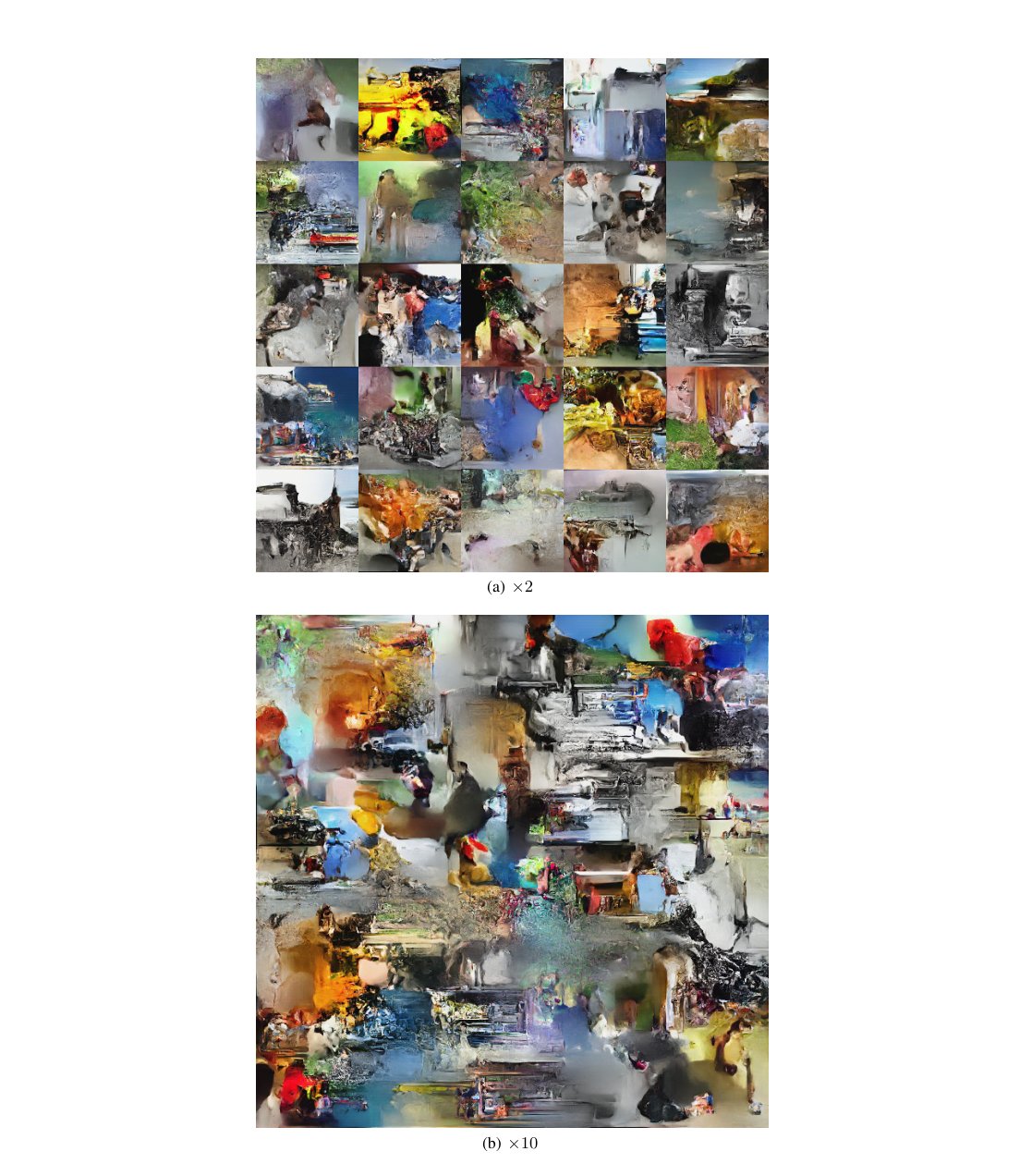
Figure 17: We generate samples a factor bigger than the training set image size on Imagenet ().
(a)
图 17:我们在 Imagenet()上生成比训练集图像尺寸大一个倍数的样本。
(a)
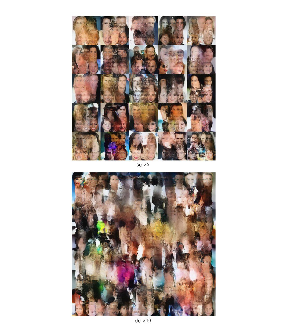
Figure 18: We generate samples a factor bigger than the training set image size on CelebA.
(a)
图 18:我们在 CelebA 上生成比训练集图像尺寸大一个倍数的样本。
(a)
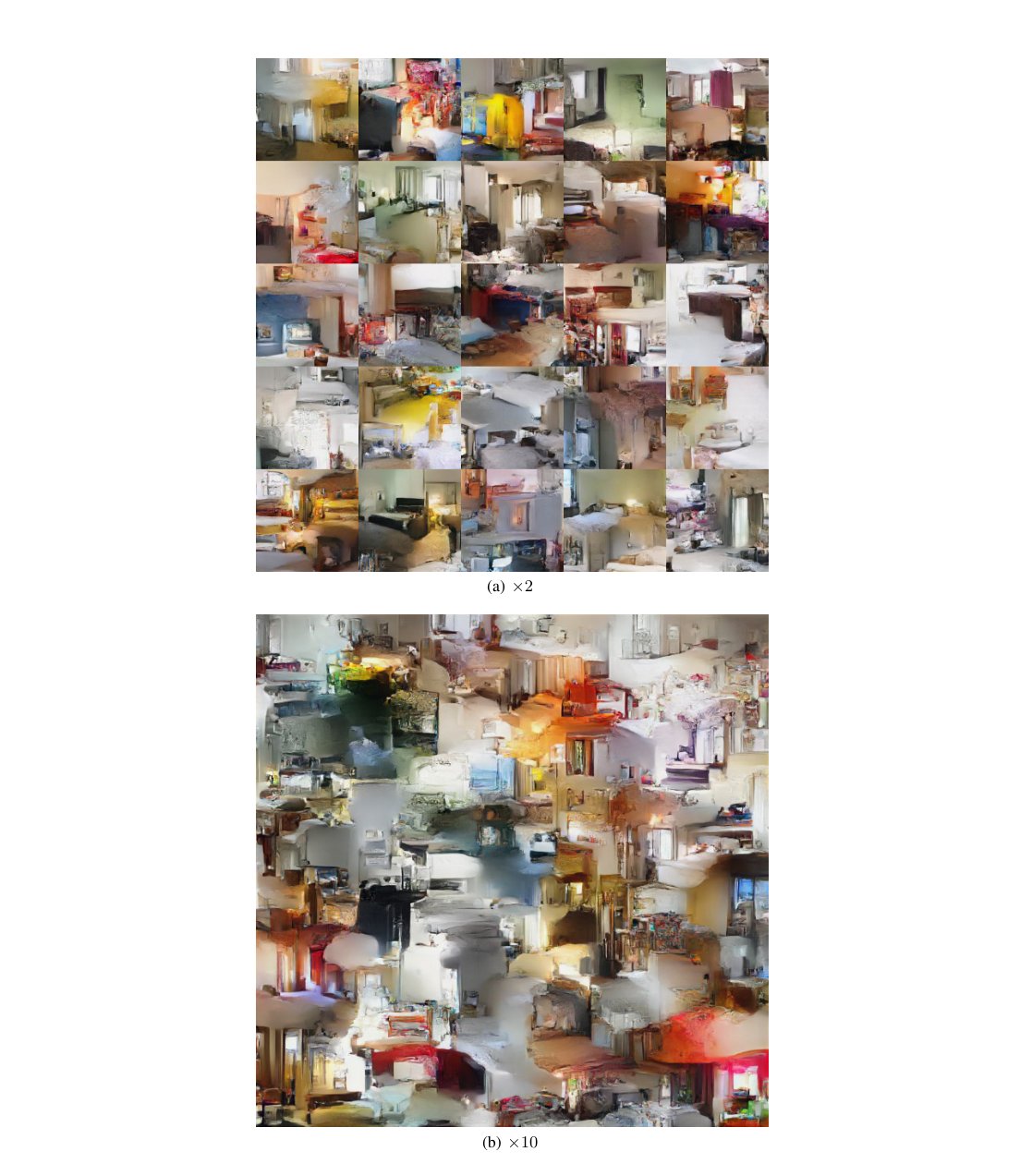
Figure 19: We generate samples a factor bigger than the training set image size on LSUN (bedroom category).
(a)
图 19:我们在 LSUN(bedroom 类别)上生成比训练集图像尺寸大一个倍数的样本。
(a)
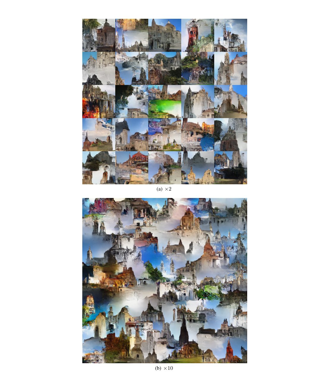
Figure 20: We generate samples a factor bigger than the training set image size on LSUN (church outdoor category).
(a)
图 20:我们在 LSUN(church outdoor 类别)上生成比训练集图像尺寸大一个倍数的样本。
(a)
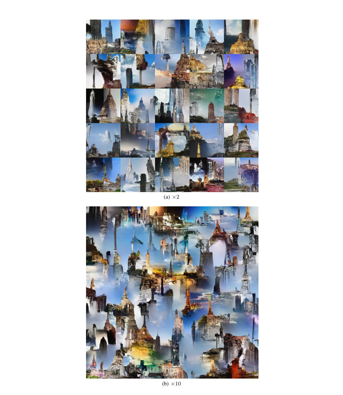
Figure 21: We generate samples a factor bigger than the training set image size on LSUN (tower category).
(a)
图 21:我们在 LSUN(tower 类别)上生成比训练集图像尺寸大一个倍数的样本。
(a)
Appendix D Latent variables semantic
附录 D 隐变量的语义
As in [22], we further try to grasp the semantic of our learned layers latent variables by doing ablation tests. We infer the latent variables and resample the lowest levels of latent variables from a standard gaussian, increasing the highest level affected by this resampling. As we can see in the following figures, the semantic of our latent space seems to be more on a graphic level rather than higher level concept. Although the heavy use of convolution improves learning by exploiting image prior knowledge, it is also likely to be responsible for this limitation.
与[22]一样,我们进一步通过对学到的各层隐变量做消融测试,来把握其语义。我们推断出隐变量,再从标准高斯中重新采样最低层次的隐变量,并逐渐提高受这次重采样影响的最高层次。正如下列各图所见,我们隐空间的语义似乎更偏向图形层面,而不是更高层的概念。尽管大量使用卷积通过利用图像先验知识改善了学习,它也很可能造成了这一局限。
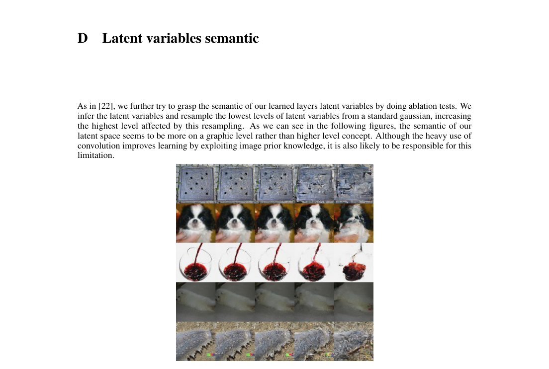
Figure 22: Conceptual compression from a model trained on Imagenet (). The leftmost column represent the original image, the subsequent columns were obtained by storing higher level latent variables and resampling the others, storing less and less as we go right. From left to right: , , , and of the latent variables are kept.
图 22:在 Imagenet()上训练的模型所做的概念压缩。最左列表示原始图像,随后各列通过保存更高层的隐变量并对其余变量重新采样得到,越往右保存得越少。从左到右:分别保留 、、、 和 的隐变量。
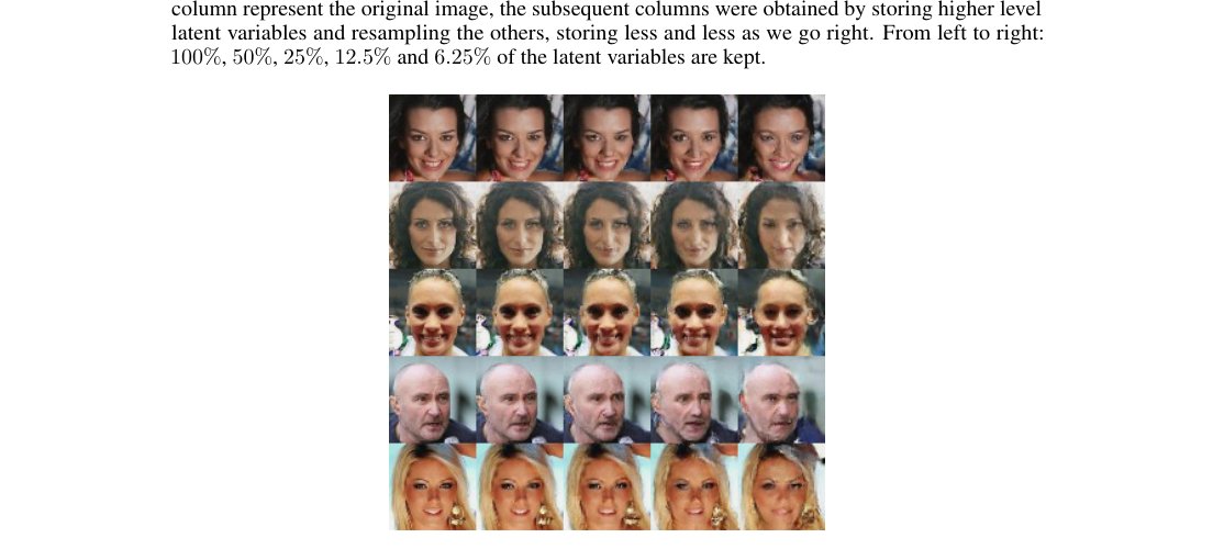
Figure 23: Conceptual compression from a model trained on CelebA. The leftmost column represent the original image, the subsequent columns were obtained by storing higher level latent variables and resampling the others, storing less and less as we go right. From left to right: , , , and of the latent variables are kept.
图 23:在 CelebA 上训练的模型所做的概念压缩。最左列表示原始图像,随后各列通过保存更高层的隐变量并对其余变量重新采样得到,越往右保存得越少。从左到右:分别保留 、、、 和 的隐变量。
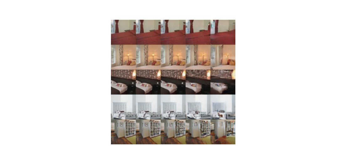
Figure 24: Conceptual compression from a model trained on LSUN (bedroom category). The leftmost column represent the original image, the subsequent columns were obtained by storing higher level latent variables and resampling the others, storing less and less as we go right. From left to right: , , , and of the latent variables are kept.
图 24:在 LSUN(bedroom 类别)上训练的模型所做的概念压缩。最左列表示原始图像,随后各列通过保存更高层的隐变量并对其余变量重新采样得到,越往右保存得越少。从左到右:分别保留 、、、 和 的隐变量。
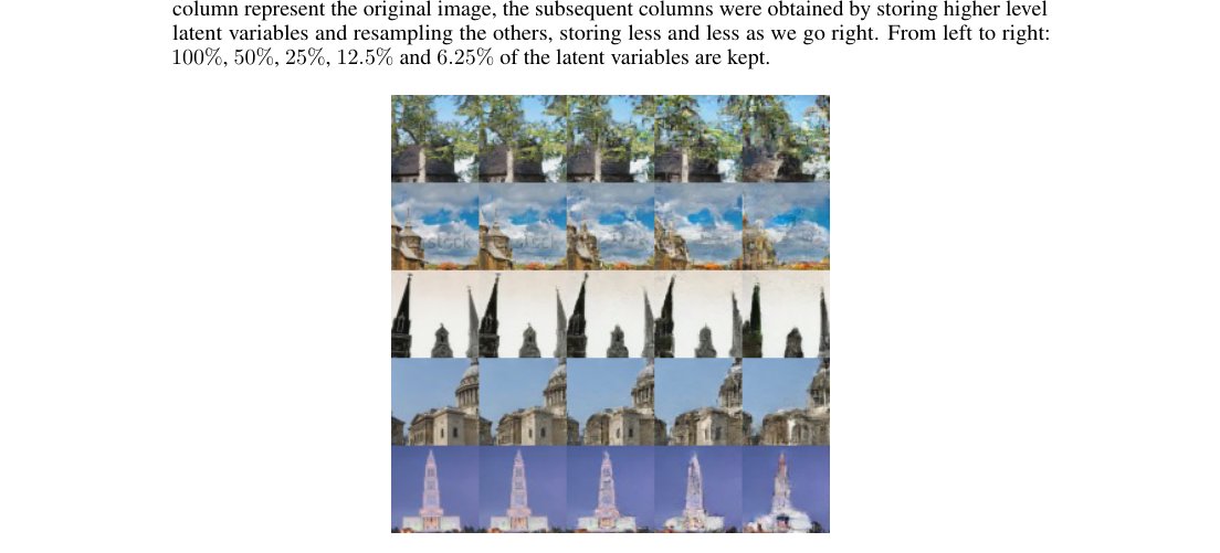
Figure 25: Conceptual compression from a model trained on LSUN (church outdoor category). The leftmost column represent the original image, the subsequent columns were obtained by storing higher level latent variables and resampling the others, storing less and less as we go right. From left to right: , , , and of the latent variables are kept.
图 25:在 LSUN(church outdoor 类别)上训练的模型所做的概念压缩。最左列表示原始图像,随后各列通过保存更高层的隐变量并对其余变量重新采样得到,越往右保存得越少。从左到右:分别保留 、、、 和 的隐变量。
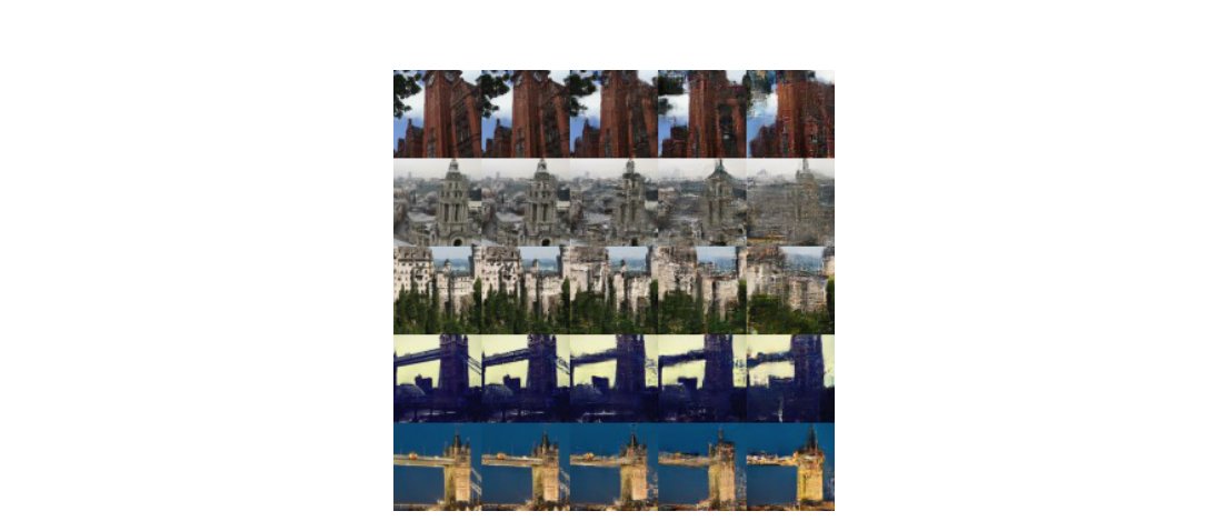
Figure 26: Conceptual compression from a model trained on LSUN (tower category). The leftmost column represent the original image, the subsequent columns were obtained by storing higher level latent variables and resampling the others, storing less and less as we go right. From left to right: , , , and of the latent variables are kept.
图 26:在 LSUN(tower 类别)上训练的模型所做的概念压缩。最左列表示原始图像,随后各列通过保存更高层的隐变量并对其余变量重新采样得到,越往右保存得越少。从左到右:分别保留 、、、 和 的隐变量。
Appendix E Batch normalization
附录 E 批归一化
We further experimented with batch normalization by using a weighted average of a moving average of the layer statistics and the current batch batch statistics ,
我们进一步实验了批归一化,使用层统计量滑动平均 与当前批次统计量 的加权平均,
where is the momentum. When using , we only propagate gradient through the current batch statistics . We observe that using this lag helps the model train with very small minibatches.
其中 是动量。当使用 时,我们只通过当前批次统计量 传播梯度。我们观察到,使用这一滞后有助于模型用非常小的小批量进行训练。
We used batch normalization with a moving average for our results on CIFAR-10.
我们在 CIFAR-10 上的结果使用了带滑动平均的批归一化。
Appendix F Attribute change
附录 F 属性更改
Additionally, we exploit the attribute information in CelebA to build a conditional model, i.e. the invertible function from image to latent variable uses the labels in to define its parameters. In order to observe the information stored in the latent variables, we choose to encode a batch of images with their original attribute and decode them using a new set of attributes , build by shuffling the original attributes inside the batch. We obtain the new images .
此外,我们利用 CelebA 中的属性信息 来建立一个条件模型,也就是说,从图像到隐变量的可逆函数 用 中的标签来定义其参数。为了观察存储在隐变量中的信息,我们选择用原始属性 编码一批图像 ,再用一组新属性 解码它们;新属性通过对该批次内的原始属性做打乱得到。我们得到新图像 。
We observe that, although the faces are changed as to respect the new attributes, several properties remain unchanged like position and background.
我们观察到,尽管面孔被改变以符合新属性,若干性质仍然保持不变,例如位置和背景。
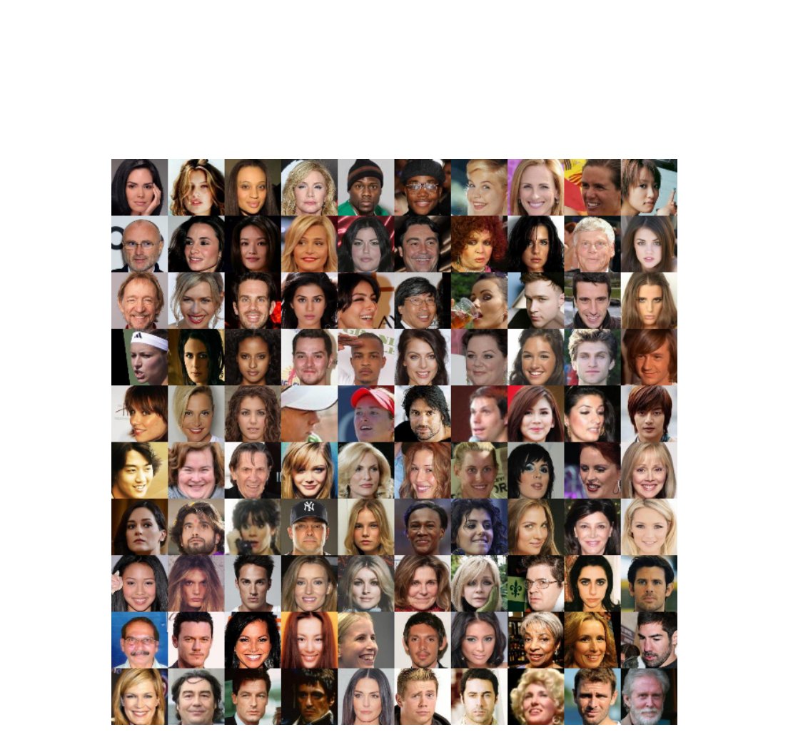
Figure 27: Examples from the CelebA dataset.
图 27:来自 CelebA 数据集的示例 。
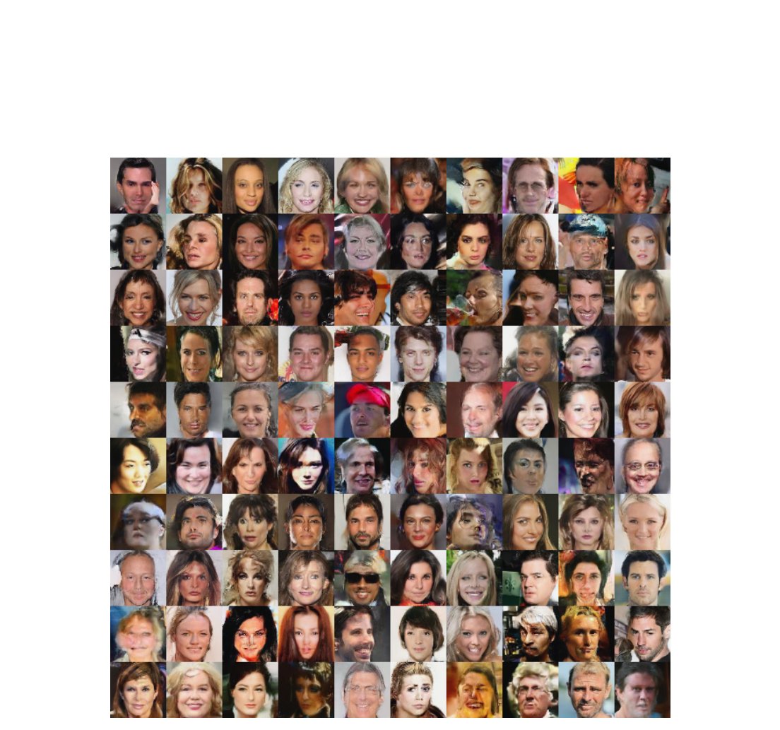
Figure 28: From a model trained on pairs of images and attributes from the CelebA dataset, we encode a batch of images with their original attributes before decoding them with a new set of attributes. We notice that the new images often share similar characteristics with those in Fig 27, including position and background.
图 28:从一个在 CelebA 数据集的图像–属性对上训练的模型出发,我们先用原始属性编码一批图像,再用一组新属性解码它们。我们注意到,新图像往往与图 27 中的图像共享相似特征,包括位置和背景。