Rainbow: Combining Improvements in Deep Reinforcement Learning

Rainbow：融合深度强化学习的多项改进

Matteo Hessel Affiliation:  DeepMind    Joseph Modayil Affiliation:  DeepMind    Hado van Hasselt Affiliation:  DeepMind    Tom Schaul Affiliation:  DeepMind    Georg Ostrovski Affiliation:  DeepMind    Will Dabney Affiliation:  DeepMind    Dan Horgan Affiliation:  DeepMind    Bilal Piot Affiliation:  DeepMind    Mohammad Azar Affiliation:  DeepMind    David Silver Affiliation:  DeepMind

Abstract

摘要

The deep reinforcement learning community has made several independent improvements to the DQN algorithm. However, it is unclear which of these extensions are complementary and can be fruitfully combined. This paper examines six extensions to the DQN algorithm and empirically studies their combination. Our experiments show that the combination provides state-of-the-art performance on the Atari 2600 benchmark, both in terms of data efficiency and final performance. We also provide results from a detailed ablation study that shows the contribution of each component to overall performance.

深度强化学习社区对 DQN 算法已提出多项彼此独立的改进。然而，这些扩展哪些互补、能否有效组合，仍不清楚。本文考察 DQN 的六种扩展，并对其组合做实证研究。实验表明，该组合在 Atari 2600 基准上同时在数据效率与最终表现上达到当时最优。我们还给出详细消融，说明各组件对整体表现的贡献。

Introduction

引言

The many recent successes in scaling reinforcement learning (RL) to complex sequential decision-making problems were kick-started by the Deep Q-Networks algorithm (DQN; ? ?, ?). Its combination of Q-learning with convolutional neural networks and experience replay enabled it to learn, from raw pixels, how to play many Atari games at human-level performance. Since then, many extensions have been proposed that enhance its speed or stability.

近期把强化学习（RL）扩展到复杂序列决策问题的诸多成功，由深度 Q 网络算法（DQN）开启。它把 Q-learning、卷积神经网络与经验回放结合，能从原始像素学会以人类水平玩许多 Atari 游戏。此后提出了大量提升其速度或稳定性的扩展。

Double DQN (DDQN; ? ?) addresses an overestimation bias of Q-learning [2010], by decoupling selection and evaluation of the bootstrap action. Prioritized experience replay [2015] improves data efficiency, by replaying more often transitions from which there is more to learn. The dueling network architecture [2016] helps to generalize across actions by separately representing state values and action advantages. Learning from multi-step bootstrap targets [1988, 1998], as used in A3C [2016], shifts the bias-variance trade-off and helps to propagate newly observed rewards faster to earlier visited states. Distributional Q-learning [2017] learns a categorical distribution of discounted returns, instead of estimating the mean. Noisy DQN [2017] uses stochastic network layers for exploration. This list is, of course, far from exhaustive.

Double DQN（DDQN）针对 Q-learning 的过估计偏差，把自举动作的选择与评估解耦。优先经验回放提高数据效率，更常回放更有学习价值的转移。对决网络架构通过分别表示状态价值与动作优势，帮助跨动作泛化。多步自举目标（如 A3C 所用）改变偏差–方差权衡，并帮助把新观测到的奖励更快传播到更早访问的状态。分布式 Q-learning 学习折扣回报的类别分布，而非估计均值。Noisy DQN 用随机网络层做探索。当然，这一清单远未穷尽。

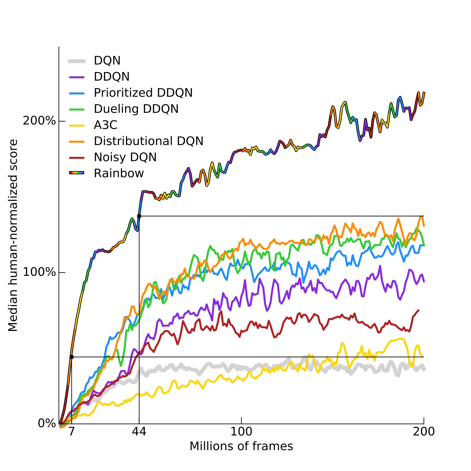
Figure 1: Median human-normalized performance across 57 Atari games. We compare our integrated agent (rainbow-colored) to DQN (grey) and six published baselines. Note that we match DQN’s best performance after 7M frames, surpass any baseline within 44M frames, and reach substantially improved final performance. Curves are smoothed with a moving average over 5 points.

图 1：57 个 Atari 游戏上的中位人类归一化表现。我们把整合智能体（彩虹色）与 DQN（灰色）及六种已发表基线比较。注意：我们在 7M 帧后匹配 DQN 的最佳表现，在 44M 帧内超过任一基线，并达到显著更好的最终表现。曲线用 5 点滑动平均平滑。

Each of these algorithms enables substantial performance improvements in isolation. Since they do so by addressing radically different issues, and since they build on a shared framework, they could plausibly be combined. In some cases this has been done: Prioritized DDQN and Dueling DDQN both use double Q-learning, and Dueling DDQN was also combined with prioritized experience replay. In this paper we propose to study an agent that combines all the aforementioned ingredients. We show how these different ideas can be integrated, and that they are indeed largely complementary. In fact, their combination results in new state-of-the-art results on the benchmark suite of 57 Atari 2600 games from the Arcade Learning Environment [2013], both in terms of data efficiency and of final performance. Finally we show results from ablation studies to help understand the contributions of the different components.

上述每种算法单独都能带来实质性能提升。它们处理截然不同的问题，又建立在同一框架上，因而有望组合。部分组合已有先例：Prioritized DDQN 与 Dueling DDQN 都使用 double Q-learning，Dueling DDQN 也曾与优先经验回放结合。本文研究把上述全部成分合入同一智能体。我们说明如何整合这些想法，并表明它们大体互补。事实上，其组合在 Arcade Learning Environment 的 57 个 Atari 2600 游戏基准上，同时在数据效率与最终表现上刷新了当时最优。最后我们给出消融结果，以理解各组件的贡献。

Background

背景

Reinforcement learning addresses the problem of an agent learning to act in an environment in order to maximize a scalar reward signal. No direct supervision is provided to the agent, for instance it is never directly told the best action.

强化学习研究智能体如何在环境中学习行动，以最大化标量奖励信号。智能体不获得直接监督，例如从不被告知最佳动作。

Agents and environments.

智能体与环境。

At each discrete time step $t=0,1,2\ldots$, the environment provides the agent with an observation $S_{t}$, the agent responds by selecting an action $A_{t}$, and then the environment provides the next reward $R_{t+1}$, discount $\gamma_{t+1}$, and state $S_{t+1}$. This interaction is formalized as a Markov Decision Process, or MDP, which is a tuple $\langle\mathcal{S},\mathcal{A},T,r,\gamma\rangle$, where $\mathcal{S}$ is a finite set of states, $\mathcal{A}$ is a finite set of actions, $T(s,a,s^{\prime})=P[S_{t+1}=s^{\prime}\mid S_{t}=s,A_{t}=a]$ is the (stochastic) transition function, $r(s,a)=\mathbb{E}[R_{t+1}\mid S_{t}=s,A_{t}=a]$ is the reward function, and $\gamma\in[0,1]$ is a discount factor. In our experiments MDPs will be episodic with a constant $\gamma_{t}=\gamma$, except on episode termination where $\gamma_{t}=0$, but the algorithms are expressed in the general form.

在每个离散时间步 $t=0,1,2\ldots$，环境向智能体提供观测 $S_{t}$，智能体选择动作 $A_{t}$，随后环境给出下一奖励 $R_{t+1}$、折扣 $\gamma_{t+1}$ 与状态 $S_{t+1}$。该交互形式化为马尔可夫决策过程（MDP），即元组 $\langle\mathcal{S},\mathcal{A},T,r,\gamma\rangle$，其中 $\mathcal{S}$ 为有限状态集，$\mathcal{A}$ 为有限动作集，$T(s,a,s^{\prime})=P[S_{t+1}=s^{\prime}\mid S_{t}=s,A_{t}=a]$ 为（随机）转移函数，$r(s,a)=\mathbb{E}[R_{t+1}\mid S_{t}=s,A_{t}=a]$ 为奖励函数，$\gamma\in[0,1]$ 为折扣因子。实验中 MDP 为回合制，常数 $\gamma_{t}=\gamma$，仅在回合终止时 $\gamma_{t}=0$，但算法以一般形式表述。

On the agent side, action selection is given by a policy $\pi$ that defines a probability distribution over actions for each state. From the state $S_{t}$ encountered at time $t$, we define the discounted return $G_{t}=\sum_{k=0}^{\infty}{\gamma_{t}^{(k)}R_{t+k+1}}$ as the discounted sum of future rewards collected by the agent, where the discount for a reward $k$ steps in the future is given by the product of discounts before that time, $\gamma_{t}^{(k)}=\prod_{i=1}^{k}\gamma_{t+i}$. An agent aims to maximize the expected discounted return by finding a good policy.

在智能体一侧，动作选择由策略 $\pi$ 给出，它定义每个状态下动作上的概率分布。从时刻 $t$ 遇到的状态 $S_{t}$ 起，折扣回报定义为 $G_{t}=\sum_{k=0}^{\infty}{\gamma_{t}^{(k)}R_{t+k+1}}$，即未来奖励的折扣和，其中 $k$ 步之后奖励的折扣为此前折扣之积 $\gamma_{t}^{(k)}=\prod_{i=1}^{k}\gamma_{t+i}$。智能体目标是通过找到好策略来最大化期望折扣回报。

The policy may be learned directly, or it may be constructed as a function of some other learned quantities. In value-based reinforcement learning, the agent learns an estimate of the expected discounted return, or value, when following a policy $\pi$ starting from a given state, $v^{\pi}(s)=E_{\pi}[G_{t}|S_{t}=s]$, or state-action pair, $q^{\pi}(s,a)=E_{\pi}[G_{t}|S_{t}=s,A_{t}=a]$. A common way of deriving a new policy from a state-action value function is to act $\epsilon$-greedily with respect to the action values. This corresponds to taking the action with the highest value (the greedy action) with probability $(1-\epsilon)$, and to otherwise act uniformly at random with probability $\epsilon$. Policies of this kind are used to introduce a form of exploration: by randomly selecting actions that are sub-optimal according to its current estimates, the agent can discover and correct its estimates when appropriate. The main limitation is that it is difficult to discover alternative courses of action that extend far into the future; this has motivated research on more directed forms of exploration.

策略可直接学习，也可构造为其他学习量的函数。在基于价值的强化学习中，智能体学习从给定状态遵循策略 $\pi$ 时期望折扣回报（价值）的估计 $v^{\pi}(s)=E_{\pi}[G_{t}|S_{t}=s]$，或状态–动作对的估计 $q^{\pi}(s,a)=E_{\pi}[G_{t}|S_{t}=s,A_{t}=a]$。由状态–动作价值函数导出新策略的常见方式，是相对动作价值做 $\epsilon$-贪婪行动：以概率 $(1-\epsilon)$ 取价值最高的动作（贪婪动作），否则以概率 $\epsilon$ 均匀随机行动。此类策略用于引入一种探索：通过随机选择按当前估计次优的动作，智能体可在适当时发现并修正估计。主要局限在于，难以发现延伸到很远未来的替代行动路径；这推动了更有向探索形式的研究。

Deep reinforcement learning and DQN.

深度强化学习与 DQN。

Large state and/or action spaces make it intractable to learn Q value estimates for each state and action pair independently. In deep reinforcement learning, we represent the various components of agents, such as policies $\pi(s,a)$ or values $q(s,a)$, with deep (i.e., multi-layer) neural networks. The parameters of these networks are trained by gradient descent to minimize some suitable loss function.

状态和/或动作空间很大时，独立学习每个状态–动作对的 Q 价值估计不可行。在深度强化学习中，我们用深度（即多层）神经网络表示智能体的各组件，如策略 $\pi(s,a)$ 或价值 $q(s,a)$。这些网络的参数通过梯度下降训练，以最小化合适的损失函数。

In DQN [2015] deep networks and reinforcement learning were successfully combined by using a convolutional neural net to approximate the action values for a given state $S_{t}$ (which is fed as input to the network in the form of a stack of raw pixel frames). At each step, based on the current state, the agent selects an action $\epsilon$-greedily with respect to the action values, and adds a transition ($S_{t},A_{t},R_{t+1},\gamma_{t+1},S_{t+1}$) to a replay memory buffer [1992], that holds the last million transitions. The parameters of the neural network are optimized by using stochastic gradient descent to minimize the loss

在 DQN 中，深度网络与强化学习通过用卷积神经网络逼近给定状态 $S_{t}$ 的动作价值而成功结合（状态以原始像素帧堆叠形式输入网络）。每一步，智能体相对动作价值做 $\epsilon$-贪婪选择动作，并把转移 $(S_{t},A_{t},R_{t+1},\gamma_{t+1},S_{t+1})$ 加入保存最近百万条转移的回放内存缓冲。神经网络参数用随机梯度下降优化，以最小化损失

$$(R_{t+1}+\gamma_{t+1}\max_{a^{\prime}}q_{\overline{\theta}}(S_{t+1},a^{\prime})-q_{\theta}(S_{t},A_{t}))^{2}\ , \tag{1}$$

where $t$ is a time step randomly picked from the replay memory. The gradient of the loss is back-propagated only into the parameters $\theta$ of the online network (which is also used to select actions); the term $\overline{\theta}$ represents the parameters of a target network; a periodic copy of the online network which is not directly optimized. The optimization is performed using RMSprop [2012], a variant of stochastic gradient descent, on mini-batches sampled uniformly from the experience replay. This means that in the loss above, the time index $t$ will be a random time index from the last million transitions, rather than the current time. The use of experience replay and target networks enables relatively stable learning of Q values, and led to super-human performance on several Atari games.

其中 $t$ 是从回放内存随机抽取的时间步。损失梯度仅回传到在线网络参数 $\theta$（该网络也用于选动作）；$\overline{\theta}$ 表示目标网络参数，即在线网络的周期性副本，不直接优化。优化用 RMSprop（随机梯度下降的一种变体），在从经验回放均匀采样的小批量上进行。因此上述损失中的时间下标 $t$ 是最近百万条转移中的随机时间下标，而非当前时间。经验回放与目标网络使 Q 价值学习相对稳定，并在若干 Atari 游戏上带来超人类表现。

Extensions to DQN

对 DQN 的扩展

DQN has been an important milestone, but several limitations of this algorithm are now known, and many extensions have been proposed. We propose a selection of six extensions that each have addressed a limitation and improved overall performance. To keep the size of the selection manageable, we picked a set of extensions that address distinct concerns (e.g., just one of the many addressing exploration).

DQN 是重要里程碑，但该算法的若干局限现已清楚，并提出了许多扩展。我们挑选六种扩展，每种针对一项局限并提升了整体表现。为使挑选规模可控，我们选取处理不同关切的扩展集合（例如在众多探索方法中只取一种）。

Double Q-learning.

Double Q-learning。

Conventional Q-learning is affected by an overestimation bias, due to the maximization step in Equation 1, and this can harm learning. Double Q-learning [2010], addresses this overestimation by decoupling, in the maximization performed for the bootstrap target, the selection of the action from its evaluation. It is possible to effectively combine this with DQN [2016], using the loss

常规 Q-learning 受过估计偏差影响，源于式 1 中的最大化步骤，可能损害学习。Double Q-learning 通过在自举目标最大化中把动作选择与评估解耦来应对过估计。可将其与 DQN 有效结合，使用损失

$$(R_{t+1}+\gamma_{t+1}q_{\overline{\theta}}(S_{t+1},\argmax_{a^{\prime}}q_{\theta}(S_{t+1},a^{\prime}))-q_{\theta}(S_{t},A_{t}))^{2}.$$

This change was shown to reduce harmful overestimations that were present for DQN, thereby improving performance.

该改动被证明可减少 DQN 中有害的过估计，从而提升表现。

Prioritized replay.

优先回放。

DQN samples uniformly from the replay buffer. Ideally, we want to sample more frequently those transitions from which there is much to learn. As a proxy for learning potential, prioritized experience replay [2015] samples transitions with probability $p_{t}$ relative to the last encountered absolute TD error:

DQN 从回放缓冲均匀采样。理想情形下，我们希望更频繁采样更有学习价值的转移。作为学习潜力的代理，优先经验回放按相对最近一次绝对TD 误差的概率 $p_{t}$ 采样转移：

$$p_{t}\propto\left|R_{t+1}+\gamma_{t+1}\max_{a^{\prime}}q_{\overline{\theta}}(S_{t+1},a^{\prime})-q_{\theta}(S_{t},A_{t})\right|^{\omega}\,,$$

where $\omega$ is a hyper-parameter that determines the shape of the distribution. New transitions are inserted into the replay buffer with maximum priority, providing a bias towards recent transitions. Note that stochastic transitions might also be favoured, even when there is little left to learn about them.

其中 $\omega$ 是决定分布形状的超参数。新转移以最大优先级插入回放缓冲，从而偏向近期转移。注意：随机转移也可能被偏爱，即便对其已几乎没什么可学。

Dueling networks.

对决网络。

The dueling network is a neural network architecture designed for value based RL. It features two streams of computation, the value and advantage streams, sharing a convolutional encoder, and merged by a special aggregator [2016]. This corresponds to the following factorization of action values:

对决网络是为基于价值的 RL 设计的神经网络架构。它有价值流与优势流两条计算流，共享卷积编码器，并由特殊聚合器合并。这对应动作价值的如下分解：

$$q_{\theta}(s,a)=v_{\eta}(f_{\xi}(s))+a_{\psi}(f_{\xi}(s),a)-\frac{\sum_{a^{\prime}}a_{\psi}(f_{\xi}(s),a^{\prime})}{N_{\text{actions}}},$$

where $\xi$, $\eta$, and $\psi$ are, respectively, the parameters of the shared encoder $f_{\xi}$, of the value stream $v_{\eta}$, and of the advantage stream $a_{\psi}$; and $\theta=\{\xi,\eta,\psi\}$ is their concatenation.

其中 $\xi$、$\eta$ 与 $\psi$ 分别是共享编码器 $f_{\xi}$、价值流 $v_{\eta}$ 与优势流 $a_{\psi}$ 的参数；$\theta=\{\xi,\eta,\psi\}$ 为其拼接。

Multi-step learning.

多步学习。

Q-learning accumulates a single reward and then uses the greedy action at the next step to bootstrap. Alternatively, forward-view multi-step targets can be used [1988]. We define the truncated $n$-step return from a given state $S_{t}$ as

Q-learning 累积单个奖励，再用下一步的贪婪动作自举。也可使用前向视角的多步目标。我们把从给定状态 $S_{t}$ 起的截断 $n$-步回报定义为

$$R_{t}^{(n)}\equiv\sum_{k=0}^{n-1}{\gamma_{t}^{(k)}R_{t+k+1}}\,. \tag{2}$$

A multi-step variant of DQN is then defined by minimizing the alternative loss,

多步变体的 DQN 于是通过最小化另一损失定义，

$$(R_{t}^{(n)}+\gamma_{t}^{(n)}\max_{a^{\prime}}q_{\overline{\theta}}(S_{t+n},a^{\prime})-q_{\theta}(S_{t},A_{t}))^{2}.$$

Multi-step targets with suitably tuned $n$ often lead to faster learning [1998].

适当调好 $n$ 的多步目标往往带来更快学习。

Distributional RL.

分布式 RL。

We can learn to approximate the distribution of returns instead of the expected return. Recently Bellemare, Dabney, and Munos (2017) proposed to model such distributions with probability masses placed on a discrete support ${\bm{z}}$, where $\bm{z}$ is a vector with $N_{\text{atoms}}\in\mathbb{N}^{+}$ atoms, defined by $z^{i}=v_{\min}+(i-1)\frac{v_{\max}-v_{\min}}{N_{\text{atoms}}-1}$ for $i\in\{1,\ldots,N_{\text{atoms}}\}$. The approximating distribution $d_{t}$ at time $t$ is defined on this support, with the probability mass $p^{i}_{\theta}(S_{t},A_{t})$ on each atom $i$, such that $d_{t}=(\bm{z},\bm{p}_{\theta}(S_{t},A_{t}))$. The goal is to update $\theta$ such that this distribution closely matches the actual distribution of returns.

我们可以学习逼近回报分布，而非期望回报。Bellemare、Dabney 与 Munos（2017）提出用放在离散支撑 ${\bm{z}}$ 上的概率质量建模此类分布，其中 $\bm{z}$ 是含 $N_{\text{atoms}}\in\mathbb{N}^{+}$ 个原子的向量，由 $z^{i}=v_{\min}+(i-1)\frac{v_{\max}-v_{\min}}{N_{\text{atoms}}-1}$（$i\in\{1,\ldots,N_{\text{atoms}}\}$）定义。时刻 $t$ 的逼近分布 $d_{t}$ 定义在该支撑上，每个原子 $i$ 上有概率质量 $p^{i}_{\theta}(S_{t},A_{t})$，使得 $d_{t}=(\bm{z},\bm{p}_{\theta}(S_{t},A_{t}))$。目标是更新 $\theta$，使该分布密切匹配真实回报分布。

To learn the probability masses, the key insight is that return distributions satisfy a variant of Bellman’s equation. For a given state $S_{t}$ and action $A_{t}$, the distribution of the returns under the optimal policy $\pi^{*}$ should match a target distribution defined by taking the distribution for the next state $S_{t+1}$ and action $a^{*}_{t+1}=\pi^{*}(S_{t+1})$, contracting it towards zero according to the discount, and shifting it by the reward (or distribution of rewards, in the stochastic case). A distributional variant of Q-learning is then derived by first constructing a new support for the target distribution, and then minimizing the Kullbeck-Leibler divergence between the distribution $d_{t}$ and the target distribution $d^{\prime}_{t}\equiv(R_{t+1}+\gamma_{t+1}\bm{z},~~\bm{p}_{\overline{\theta}}(S_{t+1},\overline{a}^{*}_{t+1}))$,

要学习概率质量，关键洞见是回报分布满足 Bellman 方程的一种变体。对给定状态 $S_{t}$ 与动作 $A_{t}$，最优策略 $\pi^{*}$ 下的回报分布应匹配如下目标分布：取下一状态 $S_{t+1}$ 与动作 $a^{*}_{t+1}=\pi^{*}(S_{t+1})$ 的分布，按折扣向零收缩，再按奖励（或随机情形下的奖励分布）平移。分布式 Q-learning 变体于是先构造目标分布的新支撑，再最小化分布 $d_{t}$ 与目标分布 $d^{\prime}_{t}\equiv(R_{t+1}+\gamma_{t+1}\bm{z},~~\bm{p}_{\overline{\theta}}(S_{t+1},\overline{a}^{*}_{t+1}))$ 之间的 Kullback–Leibler 散度，

$$D_{\text{KL}}(\Phi_{\bm{z}}d^{\prime}_{t}||d_{t})\,. \tag{3}$$

Here $\Phi_{\bm{z}}$ is a L2-projection of the target distribution onto the fixed support $\bm{z}$, and $\overline{a}^{*}_{t+1}=\argmax_{a}q_{\overline{\theta}}(S_{t+1},a)$ is the greedy action with respect to the mean action values $q_{\overline{\theta}}(S_{t+1},a)=\bm{z}^{\top}\bm{p}_{\theta}(S_{t+1},a)$ in state $S_{t+1}$.

这里 $\Phi_{\bm{z}}$ 是目标分布到固定支撑 $\bm{z}$ 的 L2 投影，$\overline{a}^{*}_{t+1}=\argmax_{a}q_{\overline{\theta}}(S_{t+1},a)$ 是状态 $S_{t+1}$ 上相对均值动作价值 $q_{\overline{\theta}}(S_{t+1},a)=\bm{z}^{\top}\bm{p}_{\theta}(S_{t+1},a)$ 的贪婪动作。

As in the non-distributional case, we can use a frozen copy of the parameters $\overline{\theta}$ to construct the target distribution. The parametrized distribution can be represented by a neural network, as in DQN, but with $N_{\text{atoms}}\times N_{\text{actions}}$ outputs. A softmax is applied independently for each action dimension of the output to ensure that the distribution for each action is appropriately normalized.

与非分布式情形一样，可用冻结参数副本 $\overline{\theta}$ 构造目标分布。参数化分布可用类似 DQN 的神经网络表示，但有 $N_{\text{atoms}}\times N_{\text{actions}}$ 个输出。对输出的每个动作维独立施加 softmax，以确保每个动作的分布适当归一化。

Noisy Nets.

Noisy Nets。

The limitations of exploring using $\epsilon$-greedy policies are clear in games such as Montezuma’s Revenge, where many actions must be executed to collect the first reward. Noisy Nets [2017] propose a noisy linear layer that combines a deterministic and noisy stream,

用 $\epsilon$-贪婪策略探索的局限在 Montezuma’s Revenge 等游戏中很明显：必须执行许多动作才能收到第一个奖励。Noisy Nets 提出结合确定性流与噪声流的噪声线性层，

$$\bm{y}=(\bm{b}+\textbf{W}\bm{x})+(\bm{b}_{noisy}\odot\epsilon^{b}+(\textbf{W}_{noisy}\odot\epsilon^{w})\bm{x}), \tag{4}$$

where $\epsilon^{b}$ and $\epsilon^{w}$ are random variables, and $\odot$ denotes the element-wise product. This transformation can then be used in place of the standard linear $\bm{y}=\bm{b}+\textbf{W}\bm{x}$. Over time, the network can learn to ignore the noisy stream, but will do so at different rates in different parts of the state space, allowing state-conditional exploration with a form of self-annealing.

其中 $\epsilon^{b}$ 与 $\epsilon^{w}$ 为随机变量，$\odot$ 表示逐元素积。该变换可替代标准线性 $\bm{y}=\bm{b}+\textbf{W}\bm{x}$。随时间推移，网络可学会忽略噪声流，但在状态空间不同区域以不同速率进行，从而以一种自退火形式实现状态条件探索。

The Integrated Agent

整合智能体

In this paper we integrate all the aforementioned components into a single integrated agent, which we call Rainbow.

本文将上述全部组件整合为单一智能体，称为 Rainbow。

First, we replace the 1-step distributional loss (3) with a multi-step variant. We construct the target distribution by contracting the value distribution in $S_{t+n}$ according to the cumulative discount, and shifting it by the truncated $n$-step discounted return. This corresponds to defining the target distribution as $d^{(n)}_{t}=(R^{(n)}_{t}+\gamma_{t}^{(n)}\bm{z},~~\bm{p}_{\overline{\theta}}(S_{t+n},a^{*}_{t+n}))$. The resulting loss is

首先，用多步变体替换 1 步分布式损失（3）。我们按累积折扣收缩 $S_{t+n}$ 处的价值分布，再按截断 $n$-步折扣回报平移，以构造目标分布。这对应于把目标分布定义为 $d^{(n)}_{t}=(R^{(n)}_{t}+\gamma_{t}^{(n)}\bm{z},~~\bm{p}_{\overline{\theta}}(S_{t+n},a^{*}_{t+n}))$。所得损失为

$$D_{\text{KL}}(\Phi_{\bm{z}}d_{t}^{(n)}||d_{t})\,,$$

where, again, $\Phi_{\bm{z}}$ is the projection onto $\bm{z}$.

其中同样地，$\Phi_{\bm{z}}$ 是到 $\bm{z}$ 的投影。

We combine the multi-step distributional loss with double Q-learning by using the greedy action in $S_{t+n}$ selected according to the online network as the bootstrap action $a^{*}_{t+n}$, and evaluating such action using the target network.

我们把多步分布式损失与 double Q-learning 结合：用按在线网络在 $S_{t+n}$ 选出的贪婪动作作为自举动作 $a^{*}_{t+n}$，并用目标网络评估该动作。

In standard proportional prioritized replay [2015] the absolute TD error is used to prioritize the transitions. This can be computed in the distributional setting, using the mean action values. However, in our experiments all distributional Rainbow variants prioritize transitions by the KL loss, since this is what the algorithm is minimizing:

在标准比例优先回放中，用绝对 TD 误差给转移定优先级。在分布式设定下可用均值动作价值计算。但在我们的实验中，所有分布式 Rainbow 变体按 KL 损失定优先级，因为这正是算法最小化的量：

$$p_{t}\propto\left(D_{\text{KL}}(\Phi_{\bm{z}}d_{t}^{(n)}||d_{t})\right)^{\omega}\,.$$

The KL loss as priority might be more robust to noisy stochastic environments because the loss can continue to decrease even when the returns are not deterministic.

以 KL 损失作优先级可能对噪声随机环境更稳健，因为即使回报非确定性，损失仍可继续下降。

The network architecture is a dueling network architecture adapted for use with return distributions. The network has a shared representation $f_{\xi}(s)$, which is then fed into a value stream $v_{\eta}$ with $N_{\text{atoms}}$ outputs, and into an advantage stream $a_{\xi}$ with $N_{\text{atoms}}\times N_{\text{actions}}$ outputs, where $a^{i}_{\xi}(f_{\xi}(s),a)$ will denote the output corresponding to atom $i$ and action $a$. For each atom $z^{i}$, the value and advantage streams are aggregated, as in dueling DQN, and then passed through a softmax layer to obtain the normalised parametric distributions used to estimate the returns’ distributions:

网络架构是适配回报分布的对决网络。网络有共享表示 $f_{\xi}(s)$，再分别送入有 $N_{\text{atoms}}$ 个输出的价值流 $v_{\eta}$，以及有 $N_{\text{atoms}}\times N_{\text{actions}}$ 个输出的优势流 $a_{\xi}$，其中 $a^{i}_{\xi}(f_{\xi}(s),a)$ 表示对应原子 $i$ 与动作 $a$ 的输出。对每个原子 $z^{i}$，价值流与优势流如对决 DQN 那样聚合，再经 softmax 层得到用于估计回报分布的归一化参数分布：

$$p^{i}_{\theta}(s,a)=\frac{\exp(v^{i}_{\eta}(\phi)+a^{i}_{\psi}(\phi,a)-\overline{a}^{i}_{\psi}(s))}{\sum_{j}\exp(v^{j}_{\eta}(\phi)+a^{j}_{\psi}(\phi,a)-\overline{a}^{j}_{\psi}(s))}\,,$$

where $\phi=f_{\xi}(s)$ and $\overline{a}^{i}_{\psi}(s)=\frac{1}{N_{\text{actions}}}\sum_{a^{\prime}}a^{i}_{\psi}(\phi,a^{\prime})$.

其中 $\phi=f_{\xi}(s)$，$\overline{a}^{i}_{\psi}(s)=\frac{1}{N_{\text{actions}}}\sum_{a^{\prime}}a^{i}_{\psi}(\phi,a^{\prime})$。

We then replace all linear layers with their noisy equivalent described in Equation (4). Within these noisy linear layers we use factorised Gaussian noise [2017] to reduce the number of independent noise variables.

随后用式（4）所述噪声等价物替换全部线性层。在这些噪声线性层中，我们使用因子化高斯噪声，以减少独立噪声变量数目。

Figure 2: Each plot shows, for several agents, the number of games where they have achieved at least a given fraction of human performance, as a function of time. From left to right we consider the 20%, 50%, 100%, 200% and 500% thresholds. On the first row we compare Rainbow to the baselines. On the second row we compare Rainbow to its ablations.

图 2：各图显示若干智能体达到至少某给定人类表现比例的游戏数目随时间的变化。从左到右分别考虑 20%、50%、100%、200% 与 500% 阈值。第一行把 Rainbow 与基线比较；第二行把 Rainbow 与其消融比较。

Experimental Methods

实验方法

We now describe the methods and setup used for configuring and evaluating the learning agents.

我们接下来描述配置与评测学习智能体所用的方法与设定。

Evaluation Methodology.

评测方法。

We evaluated all agents on 57 Atari 2600 games from the arcade learning environment [2013]. We follow the training and evaluation procedures of ? (?) and van Hasselt et al. (?). The average scores of the agent are evaluated during training, every 1M steps in the environment, by suspending learning and evaluating the latest agent for 500K frames. Episodes are truncated at 108K frames (or 30 minutes of simulated play), as in van Hasselt et al. (?).

我们在 arcade learning environment 的 57 个 Atari 2600 游戏上评测全部智能体。训练与评测流程遵循既有协议。智能体平均分数在训练期间每隔环境 1M 步评估一次：暂停学习，用最新智能体评测 500K 帧。回合在 108K 帧（或 30 分钟模拟游戏）处截断。

Agents’ scores are normalized, per game, so that 0% corresponds to a random agent and 100% to the average score of a human expert. Normalized scores can be aggregated across all Atari levels to compare the performance of different agents. It is common to track the median human normalized performance across all games. We also consider the number of games where the agent’s performance is above some fraction of human performance, to disentangle where improvements in the median come from. The mean human normalized performance is potentially less informative, as it is dominated by a few games (e.g., Atlantis) where agents achieve scores orders of magnitude higher than humans do.

智能体分数按游戏归一化，使 0% 对应随机智能体、100% 对应人类专家平均分数。归一化分数可跨全部 Atari 关卡聚合，以比较不同智能体。常见做法是跟踪全部游戏上的中位人类归一化表现。我们也考虑智能体表现高于某人类表现比例的游戏数目，以拆解中位提升来自何处。均值人类归一化表现信息量可能更少，因为会被少数游戏（如 Atlantis）主导，智能体在这些游戏上可比人类高出几个数量级。

Besides tracking the median performance as a function of environment steps, at the end of training we re-evaluate the best agent snapshot using two different testing regimes. In the no-ops starts regime, we insert a random number (up to 30) of no-op actions at the beginning of each episode (as we do also in training). In the human starts regime, episodes are initialized with points randomly sampled from the initial portion of human expert trajectories [2015]; the difference between the two regimes indicates the extent to which the agent has over-fit to its own trajectories.

除跟踪中位表现随环境步数变化外，训练结束时我们用两种测试机制重新评测最佳智能体快照。在 no-ops starts 机制中，我们在每回合开始插入随机数目（最多 30）的空操作（训练时也如此）。在 human starts 机制中，回合用从人类专家轨迹初始段随机采样的点初始化；两种机制之差表明智能体对其自身轨迹过拟合的程度。

Due to space constraints, we focus on aggregate results across games. However, in the appendix we provide full learning curves for all games and all agents, as well as detailed comparison tables of raw and normalized scores, in both the no-op and human starts testing regimes.

因篇幅限制，我们聚焦跨游戏的聚合结果。但在附录中，我们给出全部游戏与全部智能体的完整学习曲线，以及 no-op 与 human starts 两种测试机制下原始与归一化分数的详细对照表。

Parameter	Value
Min history to start learning	80K frames
Adam learning rate	$0.0000625$
Exploration $\epsilon$	$0.0$
Noisy Nets $\sigma_{0}$	0.5
Target Network Period	32K frames
Adam $\epsilon$	$1.5\times 10^{-4}$
Prioritization type	proportional
Prioritization exponent $\omega$	$0.5$
Prioritization importance sampling $\beta$	$0.4\rightarrow 1.0$
Multi-step returns $n$	3
Distributional atoms	$51$
Distributional min/max values	$[-10,10]$

Table 1: Rainbow hyper-parameters

Parameter	Value
Min history to start learning	80K frames
Adam learning rate	$0.0000625$
Exploration $\epsilon$	$0.0$
Noisy Nets $\sigma_{0}$	0.5
Target Network Period	32K frames
Adam $\epsilon$	$1.5\times 10^{-4}$
Prioritization type	proportional
Prioritization exponent $\omega$	$0.5$
Prioritization importance sampling $\beta$	$0.4\rightarrow 1.0$
Multi-step returns $n$	3
Distributional atoms	$51$
Distributional min/max values	$[-10,10]$

表 1：Rainbow 超参数

Hyper-parameter tuning.

超参数调优。

All Rainbow’s components have a number of hyper-parameters. The combinatorial space of hyper-parameters is too large for an exhaustive search, therefore we have performed limited tuning. For each component, we started with the values used in the paper that introduced this component, and tuned the most sensitive among hyper-parameters by manual coordinate descent.

Rainbow 的全部组件都有若干超参数。超参数组合空间过大，无法穷尽搜索，因此我们只做有限调优。对每个组件，我们从引入该组件的论文所用取值出发，再用手动坐标下降调最敏感的超参数。

DQN and its variants do not perform learning updates during the first $200K$ frames, to ensure sufficiently uncorrelated updates. We have found that, with prioritized replay, it is possible to start learning sooner, after only $80K$ frames.

DQN 及其变体在前 $200K$ 帧不做学习更新，以确保更新足够不相关。我们发现，使用优先回放后，可更早开始学习，仅需 $80K$ 帧。

DQN starts with an exploration $\epsilon$ of 1, corresponding to acting uniformly at random; it anneals the amount of exploration over the first 4M frames, to a final value of 0.1 (lowered to 0.01 in later variants). Whenever using Noisy Nets, we acted fully greedily ($\epsilon=0$), with a value of $0.5$ for the $\sigma_{0}$ hyper-parameter used to initialize the weights in the noisy stream[^1]. For agents without Noisy Nets, we used $\epsilon$-greedy but decreased the exploration rate faster than was previously used, annealing $\epsilon$ to 0.01 in the first $250K$ frames.

DQN 以探索 $\epsilon=1$ 起步，对应均匀随机行动；它在前 4M 帧内退火探索量，最终到 0.1（后期变体降到 0.01）。凡使用 Noisy Nets 时，我们完全贪婪行动（$\epsilon=0$），噪声流权重初始化超参数 $\sigma_{0}$ 取 $0.5$。对无 Noisy Nets 的智能体，我们仍用 $\epsilon$-贪婪，但比先前更快降低探索率：在前 $250K$ 帧内把 $\epsilon$ 退火到 0.01。

We used the Adam optimizer [2014], which we found less sensitive to the choice of the learning rate than RMSProp. DQN uses a learning rate of $\alpha=0.00025$ In all Rainbow’s variants we used a learning rate of $\alpha/4$, selected among $\{\alpha/2,\alpha/4,\alpha/6\}$, and a value of $1.5\times 10^{-4}$ for Adam’s $\epsilon$ hyper-parameter.

我们使用 Adam 优化器，发现它对学习率选择不如 RMSProp 敏感。DQN 用学习率 $\alpha=0.00025$。在全部 Rainbow 变体中，我们在 $\{\alpha/2,\alpha/4,\alpha/6\}$ 中选用 $\alpha/4$，并把 Adam 的 $\epsilon$ 超参数设为 $1.5\times 10^{-4}$。

For replay prioritization we used the recommended proportional variant, with priority exponent $\omega$ of $0.5$, and linearly increased the importance sampling exponent $\beta$ from 0.4 to 1 over the course of training. The priority exponent $\omega$ was tuned comparing values of $\{0.4,0.5,0.7\}$. Using the KL loss of distributional DQN as priority, we have observed that performance is very robust to the choice of $\omega$.

对回放优先级，我们用推荐的比例变体，优先级指数 $\omega$ 为 $0.5$，并把重要性采样指数 $\beta$ 在训练过程中从 0.4 线性增至 1。优先级指数 $\omega$ 在 $\{0.4,0.5,0.7\}$ 间比较。用分布式 DQN 的 KL 损失作优先级时，我们观察到表现对 $\omega$ 选择非常稳健。

The value of $n$ in multi-step learning is a sensitive hyper-parameter of Rainbow. We compared values of $n=1,\ 3,\ \text{and }5$. We observed that both $n=3$ and $5$ did well initially, but overall $n=3$ performed the best by the end.

多步学习中的 $n$ 是 Rainbow 的敏感超参数。我们比较了 $n=1$、$3$ 与 $5$。观察到 $n=3$ 与 $5$ 初期都不错，但到结束时总体 $n=3$ 最好。

The hyper-parameters (see Table 1) are identical across all 57 games, i.e., the Rainbow agent really is a single agent setup that performs well across all the games.

超参数（见表 1）在全部 57 个游戏上相同，也即 Rainbow 智能体确实是在全部游戏上都表现良好的单一智能体配置。

Analysis

分析

In this section we analyse the main experimental results. First, we show that Rainbow compares favorably to several published agents. Then we perform ablation studies, comparing several variants of the agent, each corresponding to removing a single component from Rainbow.

本节分析主要实验结果。首先说明 Rainbow 相对若干已发表智能体更优；随后做消融研究，比较从 Rainbow 去掉单一组件的若干变体。

Comparison to published baselines.

与已发表基线比较。

In Figure 1 we compare the Rainbow’s performance (measured in terms of the median human normalized score across games) to the corresponding curves for A3C, DQN, DDQN, Prioritized DDQN, Dueling DDQN, Distributional DQN, and Noisy DQN. We thank the authors of the Dueling and Prioritized agents for providing the learning curves of these, and report our own re-runs for DQN, A3C, DDQN, Distributional DQN and Noisy DQN. The performance of Rainbow is significantly better than any of the baselines, both in data efficiency, as well as in final performance. Note that we match final performance of DQN after 7M frames, surpass the best final performance of these baselines in 44M frames, and reach substantially improved final performance.

图 1 把 Rainbow 的表现（以跨游戏中位人类归一化分数衡量）与 A3C、DQN、DDQN、Prioritized DDQN、Dueling DDQN、Distributional DQN 与 Noisy DQN 的对应曲线比较。我们感谢 Dueling 与 Prioritized 智能体的作者提供学习曲线，并对 DQN、A3C、DDQN、Distributional DQN 与 Noisy DQN 报告我们自己的重跑。Rainbow 的表现显著优于任一基线，无论数据效率还是最终表现。注意：我们在 7M 帧后匹配 DQN 最终表现，在 44M 帧内超过这些基线的最佳最终表现，并达到显著更好的最终表现。

In the final evaluations of the agent, after the end of training, Rainbow achieves a median score of 223% in the no-ops regime; in the human starts regime we measured a median score of 153%. In Table 2 we compare these scores to the published median scores of the individual baselines.

训练结束后的最终评测中，Rainbow 在 no-ops 机制下达到中位分数 223%；在 human starts 机制下测得中位分数 153%。表 2 把这些分数与各单独基线已发表的中位分数比较。

Agent	no-ops	human starts
DQN	79%	68%
DDQN (*)	117%	110%
Prioritized DDQN (*)	140%	128%
Dueling DDQN (*)	151%	117%
A3C (*)	-	116%
Noisy DQN	118%	102%
Distributional DQN	164%	125%
Rainbow	223%	153%

Table 2: Median normalized scores of the best agent snapshots for Rainbow and baselines. For methods marked with an asterisk, the scores come from the corresponding publication. DQN’s scores comes from the dueling networks paper, since DQN’s paper did not report scores for all 57 games. The others scores come from our own implementations.

Agent	no-ops	human starts
DQN	79%	68%
DDQN (*)	117%	110%
Prioritized DDQN (*)	140%	128%
Dueling DDQN (*)	151%	117%
A3C (*)	-	116%
Noisy DQN	118%	102%
Distributional DQN	164%	125%
Rainbow	223%	153%

表 2：Rainbow 与基线的最佳智能体快照中位归一化分数。标星号方法的分数来自相应论文。DQN 分数来自对决网络论文，因 DQN 原文未报告全部 57 个游戏。其余分数来自我们自己的实现。

In Figure 2 (top row) we plot the number of games where an agent has reached some specified level of human normalized performance. From left to right, the subplots show on how many games the different agents have achieved 20%, 50%, 100%, 200% and 500% human normalized performance. This allows us to identify where the overall improvements in performance come from. Note that the gap in performance between Rainbow and other agents is apparent at all levels of performance: the Rainbow agent is improving scores on games where the baseline agents were already good, as well as improving in games where baseline agents are still far from human performance.

图 2（上行）绘制智能体达到某指定人类归一化表现水平的游戏数目。从左到右，子图分别显示不同智能体达到 20%、50%、100%、200% 与 500% 人类归一化表现的游戏数。这有助于识别整体提升来自何处。注意 Rainbow 与其他智能体的表现差距在所有表现水平上都很明显：Rainbow 既在基线已较好的游戏上继续抬分，也在基线仍远低于人类的游戏上改进。

Learning speed.

学习速度。

As in the original DQN setup, we ran each agent on a single GPU. The 7M frames required to match DQN’s final performance correspond to less than 10 hours of wall-clock time. A full run of 200M frames corresponds to approximately 10 days, and this varies by less than 20% between all of the discussed variants. The literature contains many alternative training setups that improve performance as a function of wall-clock time by exploiting parallelism, e.g., ? (?), ? (?), and ? (?). Properly relating the performance across such very different hardware/compute resources is non-trivial, so we focused exclusively on algorithmic variations, allowing apples-to-apples comparisons. While we consider them to be important and complementary, we leave questions of scalability and parallelism to future work.

与原始 DQN 设定一样，我们在单块 GPU 上运行每个智能体。匹配 DQN 最终表现所需的 7M 帧对应不到 10 小时墙钟时间。完整跑完 200M 帧约对应 10 天，所讨论全部变体之间相差不到 20%。文献中有许多通过利用并行改善墙钟时间表现的替代训练设定。跨如此不同的硬件/计算资源恰当关联表现并非易事，因此我们只聚焦算法变体，以便做公平比较。尽管我们认为可扩展性与并行性重要且互补，我们把这些问题留给未来工作。

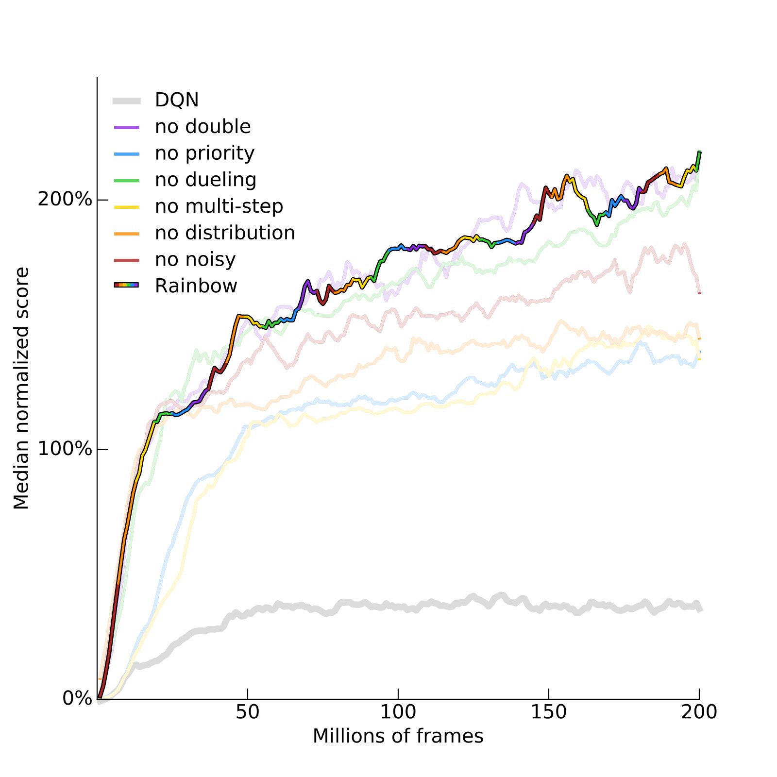
Figure 3: Median human-normalized performance across 57 Atari games, as a function of time. We compare our integrated agent (rainbow-colored) to DQN (gray) and to six different ablations (dashed lines). Curves are smoothed with a moving average over 5 points.

图 3：57 个 Atari 游戏上中位人类归一化表现随时间变化。我们把整合智能体（彩虹色）与 DQN（灰色）及六种不同消融（虚线）比较。曲线用 5 点滑动平均平滑。

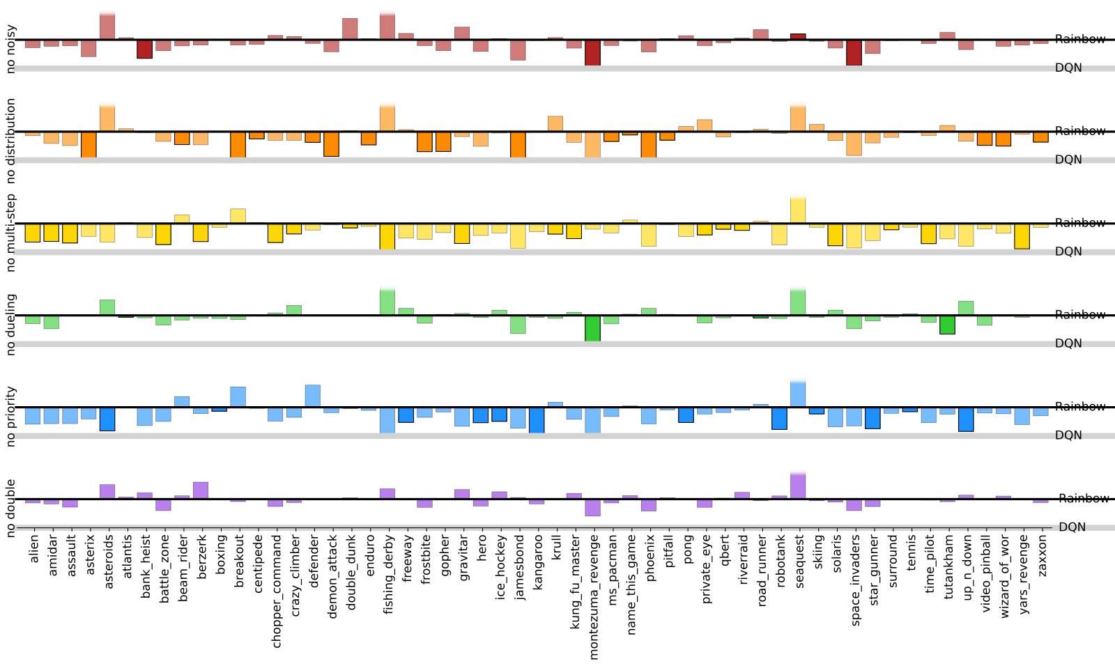
Figure 4: Performance drops of ablation agents on all 57 Atari games. Performance is the area under the learning curve, normalized relative to the Rainbow agent and DQN. Two games where DQN outperforms Rainbow are omitted. The ablation leading to the strongest drop is highlighted for each game. The removal of either prioritization or multi-step learning reduces performance across most games, but the contribution of each component varies substantially per game.

图 4：消融智能体在全部 57 个 Atari 游戏上的表现下降。表现为学习曲线下面积，相对 Rainbow 智能体与 DQN 归一化。省略 DQN 优于 Rainbow 的两款游戏。每款游戏突出导致最强下降的消融。去掉优先化或多步学习会在多数游戏上降低表现，但各组件贡献按游戏差异很大。

Ablation studies.

消融研究。

Since Rainbow integrates several different ideas into a single agent, we conducted additional experiments to understand the contribution of the various components, in the context of this specific combination.

由于 Rainbow 把若干不同想法整合进单一智能体，我们做了额外实验，以理解在此特定组合中各组件的贡献。

To gain a better understanding of the contribution of each component to the Rainbow agent, we performed ablation studies. In each ablation, we removed one component from the full Rainbow combination. Figure 3 shows a comparison for median normalized score of the full Rainbow to six ablated variants. Figure 2 (bottom row) shows a more detailed breakdown of how these ablations perform relative to different thresholds of human normalized performance, and Figure 4 shows the gain or loss from each ablation for every game, averaged over the full learning run.

为更好理解每个组件对 Rainbow 智能体的贡献，我们做了消融研究。每次消融从完整 Rainbow 组合中去掉一个组件。图 3 比较完整 Rainbow 与六种消融变体的中位归一化分数。图 2（下行）更细地展示这些消融相对不同人类归一化表现阈值的表现，图 4 展示每个消融在每款游戏上相对完整学习运行平均的增益或损失。

Prioritized replay and multi-step learning were the two most crucial components of Rainbow, in that removing either component caused a large drop in median performance. Unsurprisingly, the removal of either of these hurt early performance. Perhaps more surprisingly, the removal of multi-step learning also hurt final performance. Zooming in on individual games (Figure 4), we see both components helped almost uniformly across games (the full Rainbow performed better than either ablation in 53 games out of 57).

优先回放与多步学习是 Rainbow 最关键的两个组件：去掉任一都会导致中位表现大幅下降。不出所料，去掉任一都会损害早期表现。或许更令人惊讶的是，去掉多步学习也会损害最终表现。放大到单款游戏（图 4），我们看到这两个组件几乎在所有游戏上都有帮助（完整 Rainbow 在 57 款中的 53 款上优于任一消融）。

Distributional Q-learning ranked immediately below the previous techniques for relevance to the agent’s performance. Notably, in early learning no difference is apparent, as shown in Figure 3, where for the first 40 million frames the distributional-ablation performed as well as the full agent. However, without distributions, the performance of the agent then started lagging behind. When the results are separated relatively to human performance in Figure 2, we see that the distributional-ablation primarily seems to lags on games that are above human level or near it.

分布式 Q-learning 对智能体表现的重要性紧随其后。值得注意的是，早期学习看不出差异，如图 3 所示：前 4000 万帧内，去掉分布的消融与完整智能体表现相当。但没有分布后，智能体表现开始落后。当图 2 按相对人类表现拆分结果时，去掉分布的消融主要似乎在高于或接近人类水平的游戏上落后。

In terms of median performance, the agent performed better when Noisy Nets were included; when these are removed and exploration is delegated to the traditional $\epsilon$-greedy mechanism, performance was worse in aggregate (red line in Figure 3). While the removal of Noisy Nets produced a large drop in performance for several games, it also provided small increases in other games (Figure 4).

就中位表现而言，纳入 Noisy Nets 时智能体更好；去掉它们并把探索交给传统 $\epsilon$-贪婪机制时，总体表现更差（图 3 红线）。去掉 Noisy Nets 在若干游戏上造成大幅下降，但在另一些游戏上也带来小幅提升（图 4）。

In aggregate, we did not observe a significant difference when removing the dueling network from the full Rainbow. The median score, however, hides the fact that the impact of Dueling differed between games, as shown by Figure 4. Figure 2 shows that Dueling perhaps provided some improvement on games with above-human performance levels (# games $>200\%$), and some degradation on games with sub-human performance (# games $>20\%$).

总体而言，从完整 Rainbow 去掉对决网络时，我们未观察到显著差异。但中位分数掩盖了对决影响因游戏而异这一事实，如图 4 所示。图 2 显示，对决或许在高于人类表现水平的游戏上有所改进（游戏数 $>200\%$），在低于人类表现的游戏上有所退化（游戏数 $>20\%$）。

Also in the case of double Q-learning, the observed difference in median performance (Figure 3) is limited, with the component sometimes harming or helping depending on the game (Figure 4). To further investigate the role of double Q-learning, we compared the predictions of our trained agents to the actual discounted returns computed from clipped rewards. Comparing Rainbow to the agent where double Q-learning was ablated, we observed that the actual returns are often higher than $10$ and therefore fall outside the support of the distribution, spanning from $-10$ to $+10$. This leads to underestimated returns, rather than overestimations. We hypothesize that clipping the values to this constrained range counteracts the overestimation bias of Q-learning. Note, however, that the importance of double Q-learning may increase if the support of the distributions is expanded.

对 double Q-learning，中位表现上的观测差异（图 3）有限，该组件有时伤害、有时帮助，取决于游戏（图 4）。为进一步考察 double Q-learning 的作用，我们把训练好的智能体预测与由裁剪奖励计算的真实折扣回报比较。比较 Rainbow 与去掉 double Q-learning 的智能体时，我们观察到真实回报常高于 $10$，因而落在支撑 $[-10,+10]$ 之外。这导致低估回报，而非过估计。我们推测，把价值裁剪到该受限范围抵消了 Q-learning 的过估计偏差。但需注意，若扩展分布支撑，double Q-learning 的重要性可能上升。

In the appendix, for each game we show final performance and learning curves for Rainbow, its ablations, and baselines.

附录中，我们对每款游戏给出 Rainbow、其消融与基线的最终表现与学习曲线。

Discussion

讨论

We have demonstrated that several improvements to DQN can be successfully integrated into a single learning algorithm that achieves state-of-the-art performance. Moreover, we have shown that within the integrated algorithm, all but one of the components provided clear performance benefits. There are many more algorithmic components that we were not able to include, which would be promising candidates for further experiments on integrated agents. Among the many possible candidates, we discuss several below.

我们已证明对 DQN 的若干改进可成功整合进单一学习算法，并达到当时最优表现。而且，在整合算法内，除一个组件外，其余都提供了明确的表现收益。还有许多我们未能纳入的算法组件，是进一步整合智能体实验的有希望候选。在众多可能候选中，我们讨论如下若干。

We have focused here on value-based methods in the Q-learning family. We have not considered purely policy-based RL algorithms such as trust-region policy optimisation [2015], nor actor-critic methods [2016, 2016].

我们这里聚焦 Q-learning 族的基于价值方法。我们未考虑纯基于策略的 RL 算法，如信赖域策略优化，也未考虑 actor-critic 方法。

A number of algorithms exploit a sequence of data to achieve improved learning efficiency. Optimality tightening [2016] uses multi-step returns to construct additional inequality bounds, instead of using them to replace the 1-step targets used in Q-learning. Eligibility traces allow a soft combination over n-step returns [1988]. However, sequential methods all leverage more computation per gradient than the multi-step targets used in Rainbow. Furthermore, introducing prioritized sequence replay raises questions of how to store, replay and prioritise sequences.

若干算法利用数据序列以提升学习效率。Optimality tightening 用多步回报构造额外不等式界，而非用它们替换 Q-learning 所用的 1 步目标。资格迹允许对 n-步回报做软组合。但序列方法每次梯度都比 Rainbow 所用多步目标消耗更多计算。此外，引入优先序列回放会带来如何存储、回放与给序列定优先级的问题。

Episodic control [2016] also focuses on data efficiency, and was shown to be very effective in some domains. It improves early learning by using episodic memory as a complementary learning system, capable of immediately re-enacting successful action sequences.

情景控制也聚焦数据效率，并在若干领域被证明非常有效。它通过把情景记忆作为互补学习系统、能立即重演成功动作序列，来改善早期学习。

Besides Noisy Nets, numerous other exploration methods could also be useful algorithmic ingredients: among these Bootstrapped DQN [2016], intrinsic motivation [2015] and count-based exploration [2016]. Integration of these alternative components is fruitful subject for further research.

除 Noisy Nets 外，众多其他探索方法也可能成为有用算法成分：其中包括 Bootstrapped DQN、内在动机与基于计数的探索。整合这些替代组件是进一步研究的富有成效主题。

In this paper we have focused on the core learning updates, without exploring alternative computational architectures. Asynchronous learning from parallel copies of the environment, as in A3C [2016], Gorila [2015], or Evolution Strategies [2017], can be effective in speeding up learning, at least in terms of wall-clock time. Note, however, they can be less data efficient.

本文聚焦核心学习更新，未探索替代计算架构。如 A3C、Gorila 或 Evolution Strategies 那样从环境并行副本异步学习，可有效加速学习，至少就墙钟时间而言。但需注意，它们可能数据效率更低。

Hierarchical RL has also been applied with success to several complex Atari games. Among successful applications of HRL we highlight h-DQN [2016a] and Feudal Networks [2017].

分层 RL 也已成功应用于若干复杂 Atari 游戏。在 HRL 的成功应用中，我们强调 h-DQN 与 Feudal Networks。

The state representation could also be made more efficient by exploiting auxiliary tasks such as pixel control or feature control [2016], supervised predictions [2016] or successor features [2016b].

状态表示也可通过利用辅助任务（如像素控制或特征控制）、监督预测或后继特征而更高效。

To evaluate Rainbow fairly against the baselines, we have followed the common domain modifications of clipping rewards, fixed action-repetition, and frame-stacking, but these might be removed by other learning algorithm improvements. Pop-Art normalization [2016] allows reward clipping to be removed, while preserving a similar level of performance. Fine-grained action repetition [2017] enabled to learn how to repeat actions. A recurrent state network [2015] can learn a temporal state representation, replacing the fixed stack of observation frames. In general, we believe that exposing the real game to the agent is a promising direction for future research.

为公平相对基线评测 Rainbow，我们沿用了裁剪奖励、固定动作重复与帧堆叠等常见领域修改，但这些或许可由其他学习算法改进去除。Pop-Art 归一化允许去掉奖励裁剪，同时保持相近表现水平。细粒度动作重复使之能学习如何重复动作。循环状态网络可学习时间状态表示，替换固定观测帧堆叠。总体而言，我们认为把真实游戏暴露给智能体是未来研究的有希望方向。

References

参考文献

Appendix

附录

Table 3 lists the preprocessing of environment frames, rewards and discounts introduced by DQN. Table 4 lists the additional hyper-parameters that Rainbow inherits from DQN and the other baselines considered in this paper. The hyper-parameters for which Rainbow uses non standard settings are instead listed in the main text. In the subsequent pages, we list the tables showing, for each game, the score achieved by Rainbow and several baselines in both the no-ops regime (Table 6) and the human-starts regime (Table 5). In Figures 5 and 6 we also plot, for each game, the learning curves of Rainbow, several baselines, and all ablation experiments. These learning curves are smoothed with a moving average over a window of 10.

表 3 列出 DQN 引入的环境帧、奖励与折扣预处理。表 4 列出 Rainbow 从 DQN 与本文考虑的其他基线继承的额外超参数。Rainbow 使用非标准设定的超参数则列于正文。随后各页列出表格，展示 Rainbow 与若干基线在 no-ops 机制（表 6）与 human-starts 机制（表 5）下每款游戏的分数。图 5 与图 6 还绘制 Rainbow、若干基线与全部消融实验在每款游戏上的学习曲线。这些学习曲线用窗口为 10 的滑动平均平滑。

Hyper-parameter	value
Grey-scaling	True
Observation down-sampling	(84, 84)
Frames stacked	4
Action repetitions	4
Reward clipping	[-1, 1]
Terminal on loss of life	True
Max frames per episode	108K

Table 3: Preprocessing: the values of these hyper-parameters are the same used by DQN and it’s variants. They are here listed for completeness. Observations are grey-scaled and rescaled to $84\times 84$ pixels. 4 consecutive frames are concatenated as each state’s representation. Each action selected by the agent is repeated for 4 times. Rewards are clipped between $-1,+1$. In games where the player has multiple lives, transitions associated to the loss of a life are considered terminal. All episodes are capped after 108K frames.

Hyper-parameter	value
Grey-scaling	True
Observation down-sampling	(84, 84)
Frames stacked	4
Action repetitions	4
Reward clipping	[-1, 1]
Terminal on loss of life	True
Max frames per episode	108K

表 3：预处理：这些超参数取值与 DQN 及其变体相同，此处列出以供完整。观测灰度化并缩放到 $84\times 84$ 像素。连续 4 帧拼接为每个状态的表示。智能体所选每个动作重复 4 次。奖励裁剪到 $-1,+1$。在玩家有多条命的游戏中，与失命相关的转移视为终止。全部回合在 108K 帧后封顶。

Hyper-parameter	value
Q network: channels	32, 64, 64
Q network: filter size	$8\times 8,4\times 4,3\times 3$
Q network: stride	4, 2, 1
Q network: hidden units	512
Q network: output units	Number of actions
Discount factor	0.99
Memory size	1M transitions
Replay period	every 4 agent steps
Minibatch size	32

Table 4: Additional hyper-parameters: the values of these hyper-parameters are the same used by DQN and it’s variants. The network has 3 convolutional layers: with 32, 64 and 64 channels. The layers use $8\times 8$, $4\times 4$, $3\times 3$ filters with strides of 4, 2, 1, respectively. The value and advantage streams of the dueling architecture have both a hidden layer with 512 units. The output layer of the network has a number of units equal to the number of actions available in the game. We use a discount factor of 0.99, which is set to 0 on terminal transitions. We perform a learning update every 4 agent steps, using mini-batches of 32 transitions.

Hyper-parameter	value
Q network: channels	32, 64, 64
Q network: filter size	$8\times 8,4\times 4,3\times 3$
Q network: stride	4, 2, 1
Q network: hidden units	512
Q network: output units	Number of actions
Discount factor	0.99
Memory size	1M transitions
Replay period	every 4 agent steps
Minibatch size	32

表 4：额外超参数：这些超参数取值与 DQN 及其变体相同。网络有 3 个卷积层：通道数分别为 32、64 与 64。各层分别使用 $8\times 8$、$4\times 4$、$3\times 3$ 滤波器，步幅为 4、2、1。对决架构的价值流与优势流都有 512 单元的隐层。网络输出层单元数等于游戏可用动作数。我们使用折扣因子 0.99，在终止转移上设为 0。每 4 个智能体步做一次学习更新，小批量大小为 32。

Game	DQN	A3C	DDQN	Prior. DDQN	Duel. DDQN	Distrib. DQN	Noisy DQN	Rainbow
alien	634.0	518.4	1033.4	900.5	1,486.5	1,997.5	533.3	6,022.9
amidar	178.4	263.9	169.1	218.4	172.7	237.7	148.0	202.8
assault	3489.3	5474.9	6060.8	7,748.5	3,994.8	5,101.3	5,124.3	14,491.7
asterix	3170.5	22140.5	16837.0	31,907.5	15,840.0	395,599.5	8,277.3	280,114.0
asteroids	1458.7	4474.5	1193.2	1,654.0	2,035.4	2,071.7	4,078.1	2,249.4
atlantis	292491.0	911,091.0	319688.0	593,642.0	445,360.0	289,803.0	303,666.5	814,684.0
bank_heist	312.7	970.1	886.0	816.8	1,129.3	835.6	955.0	826.0
battle_zone	23750.0	12950.0	24740.0	29,100.0	31,320.0	32,250.0	26,985.0	52,040.0
beam_rider	9743.2	22707.9	17417.2	26,172.7	14,591.3	15,002.4	15,241.5	21,768.5
berzerk	493.4	817.9	1011.1	1,165.6	910.6	1,000.0	670.8	1,793.4
bowling	56.5	35.1	69.6	65.8	65.7	76.8	79.3	39.4
boxing	70.3	59.8	73.5	68.6	77.3	62.1	66.3	54.9
breakout	354.5	681.9	368.9	371.6	411.6	548.7	423.3	379.5
centipede	3973.9	3755.8	3853.5	3,421.9	4,881.0	7,476.9	4,214.4	7,160.9
chopper_command	5017.0	7021.0	3495.0	6,604.0	3,784.0	9,600.5	8,778.5	10,916.0
crazy_climber	98128.0	112646.0	113782.0	131,086.0	124,566.0	154,416.5	98,576.5	143,962.0
defender	15917.5	56533.0	27510.0	21,093.5	33,996.0	32,246.0	18,037.5	47,671.3
demon_attack	12550.7	113,308.4	69803.4	73,185.8	56,322.8	109,856.6	25,207.8	109,670.7
double_dunk	-6.0	-0.1	-0.3	2.7	-0.8	-3.7	-1.0	-0.6
enduro	626.7	-82.5	1216.6	1,884.4	2,077.4	2,133.4	1,021.5	2,061.1
fishing_derby	-1.6	18.8	3.2	9.2	-4.1	-4.9	-3.7	22.6
freeway	26.9	0.1	28.8	27.9	0.2	28.8	27.1	29.1
frostbite	496.1	190.5	1448.1	2,930.2	2,332.4	2,813.9	418.8	4,141.1
gopher	8190.4	10022.8	15253.0	57,783.8	20,051.4	27,778.3	13,131.0	72,595.7
gravitar	298.0	303.5	200.5	218.0	297.0	422.0	250.5	567.5
hero	14992.9	32464.1	14892.5	20,506.4	15,207.9	28,554.2	2,454.2	50,496.8
ice_hockey	-1.6	-2.8	-2.5	-1.0	-1.3	-0.1	-2.4	-0.7
kangaroo	4496.0	94.0	11204.0	10,241.0	10,334.0	9,555.5	7,465.0	10,841.0
krull	6206.0	5560.0	6796.1	7,406.5	8,051.6	6,757.8	6,833.5	6,715.5
kung_fu_master	20882.0	28819.0	30207.0	31,244.0	24,288.0	33,890.0	27,921.0	28,999.8
montezuma_revenge	47.0	67.0	42.0	13.0	22.0	130.0	55.0	154.0
ms_pacman	1092.3	653.7	1241.3	1,824.6	2,250.6	2,064.1	1,012.1	2,570.2
name_this_game	6738.8	10476.1	8960.3	11,836.1	11,185.1	11,382.3	7,186.4	11,686.5
phoenix	7484.8	52894.1	12366.5	27,430.1	20,410.5	31,358.3	15,505.0	103,061.6
pitfall	-113.2	-78.5	-186.7	-14.8	-46.9	-342.8	-154.4	-37.6
pong	18.0	5.6	19.1	18.9	18.8	18.9	18.0	19.0
private_eye	207.9	206.9	-575.5	179.0	292.6	5,717.5	5,955.4	1,704.4
qbert	9271.5	15148.8	11020.8	11,277.0	14,175.8	15,035.9	9,176.6	18,397.6
road_runner	35215.0	34216.0	43156.0	56,990.0	58,549.0	56,086.0	35,376.5	54,261.0
robotank	58.7	32.8	59.1	55.4	62.0	49.8	50.9	55.2
seaquest	4216.7	2355.4	14498.0	39,096.7	37,361.6	3,275.4	2,353.1	19,176.0
skiing	-12142.1	-10911.1	-11490.4	-10,852.8	-11,928.0	-13,247.7	-13,905.9	-11,685.8
solaris	1295.4	1956.0	810.0	2,238.2	1,768.4	2,530.2	2,608.2	2,860.7
space_invaders	1293.8	15,730.5	2628.7	9,063.0	5,993.1	6,368.6	1,697.2	12,629.0
star_gunner	52970.0	138218.0	58365.0	51,959.0	90,804.0	67,054.5	31,864.5	123,853.0
surround	-6.0	-9.7	1.9	-0.9	4.0	4.5	-3.1	7.0
tennis	11.1	-6.3	-7.8	-2.0	4.4	22.6	-2.1	-2.2
time_pilot	4786.0	12,679.0	6608.0	7,448.0	6,601.0	7,684.5	5,311.0	11,190.5
tutankham	45.6	156.3	92.2	33.6	48.0	124.3	123.3	126.9
venture	136.0	23.0	21.0	244.0	200.0	462.0	10.5	45.0
video_pinball	154414.1	331628.1	367823.7	374,886.9	110,976.2	455,052.7	241,851.7	506,817.2
wizard_of_wor	1609.0	17,244.0	6201.0	7,451.0	7,054.0	11,824.5	4,796.5	14,631.5
yars_revenge	4577.5	7157.5	6270.6	5,965.1	25,976.5	8,267.7	5,487.3	93,007.9
zaxxon	4412.0	24,622.0	8593.0	9,501.0	10,164.0	15,130.0	7,650.5	19,658.0

Table 5: Human Starts evaluation regime: Raw scores across all games, averaged over 200 testing episodes, from the agent snapshot that obtained the highest score during training. We report the published scores for DQN, A3C, DDQN, Dueling DDQN, and Prioritized DDQN. For Distributional DQN and Rainbow we report our own evaluations of the agents.

表 5：human starts 机制下 Rainbow 与若干基线在各游戏上的分数（节选；原文表格较长）。

Game	DQN	A3C	DDQN	Prior. DDQN	Duel. DDQN	Distrib. DQN	Noisy DQN	Rainbow
alien	634.0	518.4	1033.4	900.5	1,486.5	1,997.5	533.3	6,022.9
amidar	178.4	263.9	169.1	218.4	172.7	237.7	148.0	202.8
assault	3489.3	5474.9	6060.8	7,748.5	3,994.8	5,101.3	5,124.3	14,491.7
asterix	3170.5	22140.5	16837.0	31,907.5	15,840.0	395,599.5	8,277.3	280,114.0
asteroids	1458.7	4474.5	1193.2	1,654.0	2,035.4	2,071.7	4,078.1	2,249.4
atlantis	292491.0	911,091.0	319688.0	593,642.0	445,360.0	289,803.0	303,666.5	814,684.0
bank_heist	312.7	970.1	886.0	816.8	1,129.3	835.6	955.0	826.0
battle_zone	23750.0	12950.0	24740.0	29,100.0	31,320.0	32,250.0	26,985.0	52,040.0
beam_rider	9743.2	22707.9	17417.2	26,172.7	14,591.3	15,002.4	15,241.5	21,768.5
berzerk	493.4	817.9	1011.1	1,165.6	910.6	1,000.0	670.8	1,793.4
bowling	56.5	35.1	69.6	65.8	65.7	76.8	79.3	39.4
boxing	70.3	59.8	73.5	68.6	77.3	62.1	66.3	54.9
breakout	354.5	681.9	368.9	371.6	411.6	548.7	423.3	379.5
centipede	3973.9	3755.8	3853.5	3,421.9	4,881.0	7,476.9	4,214.4	7,160.9
chopper_command	5017.0	7021.0	3495.0	6,604.0	3,784.0	9,600.5	8,778.5	10,916.0
crazy_climber	98128.0	112646.0	113782.0	131,086.0	124,566.0	154,416.5	98,576.5	143,962.0
defender	15917.5	56533.0	27510.0	21,093.5	33,996.0	32,246.0	18,037.5	47,671.3
demon_attack	12550.7	113,308.4	69803.4	73,185.8	56,322.8	109,856.6	25,207.8	109,670.7
double_dunk	-6.0	-0.1	-0.3	2.7	-0.8	-3.7	-1.0	-0.6
enduro	626.7	-82.5	1216.6	1,884.4	2,077.4	2,133.4	1,021.5	2,061.1
fishing_derby	-1.6	18.8	3.2	9.2	-4.1	-4.9	-3.7	22.6
freeway	26.9	0.1	28.8	27.9	0.2	28.8	27.1	29.1
frostbite	496.1	190.5	1448.1	2,930.2	2,332.4	2,813.9	418.8	4,141.1
gopher	8190.4	10022.8	15253.0	57,783.8	20,051.4	27,778.3	13,131.0	72,595.7
gravitar	298.0	303.5	200.5	218.0	297.0	422.0	250.5	567.5
hero	14992.9	32464.1	14892.5	20,506.4	15,207.9	28,554.2	2,454.2	50,496.8
ice_hockey	-1.6	-2.8	-2.5	-1.0	-1.3	-0.1	-2.4	-0.7
kangaroo	4496.0	94.0	11204.0	10,241.0	10,334.0	9,555.5	7,465.0	10,841.0
krull	6206.0	5560.0	6796.1	7,406.5	8,051.6	6,757.8	6,833.5	6,715.5
kung_fu_master	20882.0	28819.0	30207.0	31,244.0	24,288.0	33,890.0	27,921.0	28,999.8
montezuma_revenge	47.0	67.0	42.0	13.0	22.0	130.0	55.0	154.0
ms_pacman	1092.3	653.7	1241.3	1,824.6	2,250.6	2,064.1	1,012.1	2,570.2
name_this_game	6738.8	10476.1	8960.3	11,836.1	11,185.1	11,382.3	7,186.4	11,686.5
phoenix	7484.8	52894.1	12366.5	27,430.1	20,410.5	31,358.3	15,505.0	103,061.6
pitfall	-113.2	-78.5	-186.7	-14.8	-46.9	-342.8	-154.4	-37.6
pong	18.0	5.6	19.1	18.9	18.8	18.9	18.0	19.0
private_eye	207.9	206.9	-575.5	179.0	292.6	5,717.5	5,955.4	1,704.4
qbert	9271.5	15148.8	11020.8	11,277.0	14,175.8	15,035.9	9,176.6	18,397.6
road_runner	35215.0	34216.0	43156.0	56,990.0	58,549.0	56,086.0	35,376.5	54,261.0
robotank	58.7	32.8	59.1	55.4	62.0	49.8	50.9	55.2
seaquest	4216.7	2355.4	14498.0	39,096.7	37,361.6	3,275.4	2,353.1	19,176.0
skiing	-12142.1	-10911.1	-11490.4	-10,852.8	-11,928.0	-13,247.7	-13,905.9	-11,685.8
solaris	1295.4	1956.0	810.0	2,238.2	1,768.4	2,530.2	2,608.2	2,860.7
space_invaders	1293.8	15,730.5	2628.7	9,063.0	5,993.1	6,368.6	1,697.2	12,629.0
star_gunner	52970.0	138218.0	58365.0	51,959.0	90,804.0	67,054.5	31,864.5	123,853.0
surround	-6.0	-9.7	1.9	-0.9	4.0	4.5	-3.1	7.0
tennis	11.1	-6.3	-7.8	-2.0	4.4	22.6	-2.1	-2.2
time_pilot	4786.0	12,679.0	6608.0	7,448.0	6,601.0	7,684.5	5,311.0	11,190.5
tutankham	45.6	156.3	92.2	33.6	48.0	124.3	123.3	126.9
venture	136.0	23.0	21.0	244.0	200.0	462.0	10.5	45.0
video_pinball	154414.1	331628.1	367823.7	374,886.9	110,976.2	455,052.7	241,851.7	506,817.2
wizard_of_wor	1609.0	17,244.0	6201.0	7,451.0	7,054.0	11,824.5	4,796.5	14,631.5
yars_revenge	4577.5	7157.5	6270.6	5,965.1	25,976.5	8,267.7	5,487.3	93,007.9
zaxxon	4412.0	24,622.0	8593.0	9,501.0	10,164.0	15,130.0	7,650.5	19,658.0

Table 5: Human Starts evaluation regime: Raw scores across all games, averaged over 200 testing episodes, from the agent snapshot that obtained the highest score during training. We report the published scores for DQN, A3C, DDQN, Dueling DDQN, and Prioritized DDQN. For Distributional DQN and Rainbow we report our own evaluations of the agents.

Game	DQN	DDQN	Prior. DDQN	Duel. DDQN	Distrib. DQN	Noisy DQN	Rainbow
alien	1620.0	3747.7	6,648.6	4,461.4	4,055.8	2,394.9	9,491.7
amidar	978.0	1793.3	2,051.8	2,354.5	1,267.9	1,608.0	5,131.2
assault	4280.0	5393.2	7,965.7	4,621.0	5,909.0	5,198.6	14,198.5
asterix	4359.0	17356.5	41,268.0	28,188.0	400,529.5	12,403.8	428,200.3
asteroids	1364.5	734.7	1,699.3	2,837.7	2,354.7	4,814.1	2,712.8
atlantis	279987.0	106056.0	427,658.0	382,572.0	273,895.0	329,010.0	826,659.5
bank_heist	455.0	1030.6	1,126.8	1,611.9	1,056.7	1,323.0	1,358.0
battle_zone	29900.0	31700.0	38,130.0	37,150.0	41,145.0	32,050.0	62,010.0
beam_rider	8627.5	13772.8	22,430.7	12,164.0	13,213.4	12,534.0	16,850.2
berzerk	585.6	1225.4	1,614.2	1,472.6	1,421.8	837.3	2,545.6
bowling	50.4	68.1	62.6	65.5	74.1	77.3	30.0
boxing	88.0	91.6	98.8	99.4	98.1	83.3	99.6
breakout	385.5	418.5	381.5	345.3	612.5	459.1	417.5
centipede	4657.7	5409.4	5,175.4	7,561.4	9,015.5	4,355.8	8,167.3
chopper_command	6126.0	5809.0	5,135.0	11,215.0	13,136.0	9,519.0	16,654.0
crazy_climber	110763.0	117282.0	183,137.0	143,570.0	178,355.0	118,768.0	168,788.5
defender	23633.0	35338.5	24,162.5	42,214.0	37,896.8	23,083.0	55,105.0
demon_attack	12149.4	58044.2	70,171.8	60,813.3	110,626.5	24,950.1	111,185.2
double_dunk	-6.6	-5.5	4.8	0.1	-3.8	-1.8	-0.3
enduro	729.0	1211.8	2,155.0	2,258.2	2,259.3	1,129.2	2,125.9
fishing_derby	-4.9	15.5	30.2	46.4	9.1	7.7	31.3
freeway	30.8	33.3	32.9	0.0	33.6	32.0	34.0
frostbite	797.4	1683.3	3,421.6	4,672.8	3,938.2	583.6	9,590.5
gopher	8777.4	14840.8	49,097.4	15,718.4	28,841.0	15,107.9	70,354.6
gravitar	473.0	412.0	330.5	588.0	681.0	443.5	1,419.3
hero	20437.8	20130.2	27,153.9	20,818.2	33,860.9	5,053.1	55,887.4
ice_hockey	-1.9	-2.7	0.3	0.5	1.3	-2.1	1.1
kangaroo	7259.0	12992.0	14,492.0	14,854.0	12,909.0	12,117.0	14,637.5
krull	8422.3	7920.5	10,263.1	11,451.9	9,885.9	9,061.9	8,741.5
kung_fu_master	26059.0	29710.0	43,470.0	34,294.0	43,009.0	34,099.0	52,181.0
montezuma_revenge	0.0	0.0	0.0	0.0	367.0	0.0	384.0
ms_pacman	3085.6	2711.4	4,751.2	6,283.5	3,769.2	2,501.6	5,380.4
name_this_game	8207.8	10616.0	13,439.4	11,971.1	12,983.6	8,332.4	13,136.0
phoenix	8485.2	12252.5	32,808.3	23,092.2	34,775.0	16,974.3	108,528.6
pitfall	-286.1	-29.9	0.0	0.0	-2.1	-18.2	0.0
pong	19.5	20.9	20.7	21.0	20.8	21.0	20.9
private_eye	146.7	129.7	200.0	103.0	15,172.9	3,966.0	4,234.0
qbert	13117.3	15088.5	18,802.8	19,220.3	16,956.0	15,276.3	33,817.5
road_runner	39544.0	44127.0	62,785.0	69,524.0	63,366.0	41,681.0	62,041.0
robotank	63.9	65.1	58.6	65.3	54.2	53.5	61.4
seaquest	5860.6	16452.7	44,417.4	50,254.2	4,754.4	2,495.4	15,898.9
skiing	-13062.3	-9021.8	-9,900.5	-8,857.4	-14,959.8	-16,307.3	-12,957.8
solaris	3482.8	3067.8	1,710.8	2,250.8	5,643.1	3,204.5	3,560.3
space_invaders	1692.3	2525.5	7,696.9	6,427.3	6,869.1	2,145.5	18,789.0
star_gunner	54282.0	60142.0	56,641.0	89,238.0	69,306.5	34,504.5	127,029.0
surround	-5.6	-2.9	2.1	4.4	6.2	-3.3	9.7
tennis	12.2	-22.8	0.0	5.1	23.6	0.0	-0.0
time_pilot	4870.0	8339.0	11,448.0	11,666.0	7,875.0	6,157.0	12,926.0
tutankham	68.1	218.4	87.2	211.4	249.4	231.6	241.0
venture	163.0	98.0	863.0	497.0	1,107.0	0.0	5.5
video_pinball	196760.4	309941.9	406,420.4	98,209.5	478,646.7	270,444.6	533,936.5
wizard_of_wor	2704.0	7492.0	10,373.0	7,855.0	15,994.5	5,432.0	17,862.5
yars_revenge	18089.9	11712.6	16,451.7	49,622.1	16,608.6	9,570.1	102,557.0
zaxxon	5363.0	10163.0	13,490.0	12,944.0	18,347.5	9,390.0	22,209.5

Table 6: No-op starts evaluation regime: Raw scores across all games, averaged over 200 testing episodes, from the agent snapshot that obtained the highest score during training. We report the published scores for DQN, DDQN, Dueling DDQN, and Prioritized DDQN. For Distributional DQN and Rainbow we report our own evaluations of the agents. A3C is not listed since the paper did not report the scores for the no-ops regime.

表 6：no-ops 机制下 Rainbow 与若干基线在各游戏上的分数（节选；原文表格较长）。

Game	DQN	DDQN	Prior. DDQN	Duel. DDQN	Distrib. DQN	Noisy DQN	Rainbow
alien	1620.0	3747.7	6,648.6	4,461.4	4,055.8	2,394.9	9,491.7
amidar	978.0	1793.3	2,051.8	2,354.5	1,267.9	1,608.0	5,131.2
assault	4280.0	5393.2	7,965.7	4,621.0	5,909.0	5,198.6	14,198.5
asterix	4359.0	17356.5	41,268.0	28,188.0	400,529.5	12,403.8	428,200.3
asteroids	1364.5	734.7	1,699.3	2,837.7	2,354.7	4,814.1	2,712.8
atlantis	279987.0	106056.0	427,658.0	382,572.0	273,895.0	329,010.0	826,659.5
bank_heist	455.0	1030.6	1,126.8	1,611.9	1,056.7	1,323.0	1,358.0
battle_zone	29900.0	31700.0	38,130.0	37,150.0	41,145.0	32,050.0	62,010.0
beam_rider	8627.5	13772.8	22,430.7	12,164.0	13,213.4	12,534.0	16,850.2
berzerk	585.6	1225.4	1,614.2	1,472.6	1,421.8	837.3	2,545.6
bowling	50.4	68.1	62.6	65.5	74.1	77.3	30.0
boxing	88.0	91.6	98.8	99.4	98.1	83.3	99.6
breakout	385.5	418.5	381.5	345.3	612.5	459.1	417.5
centipede	4657.7	5409.4	5,175.4	7,561.4	9,015.5	4,355.8	8,167.3
chopper_command	6126.0	5809.0	5,135.0	11,215.0	13,136.0	9,519.0	16,654.0
crazy_climber	110763.0	117282.0	183,137.0	143,570.0	178,355.0	118,768.0	168,788.5
defender	23633.0	35338.5	24,162.5	42,214.0	37,896.8	23,083.0	55,105.0
demon_attack	12149.4	58044.2	70,171.8	60,813.3	110,626.5	24,950.1	111,185.2
double_dunk	-6.6	-5.5	4.8	0.1	-3.8	-1.8	-0.3
enduro	729.0	1211.8	2,155.0	2,258.2	2,259.3	1,129.2	2,125.9
fishing_derby	-4.9	15.5	30.2	46.4	9.1	7.7	31.3
freeway	30.8	33.3	32.9	0.0	33.6	32.0	34.0
frostbite	797.4	1683.3	3,421.6	4,672.8	3,938.2	583.6	9,590.5
gopher	8777.4	14840.8	49,097.4	15,718.4	28,841.0	15,107.9	70,354.6
gravitar	473.0	412.0	330.5	588.0	681.0	443.5	1,419.3
hero	20437.8	20130.2	27,153.9	20,818.2	33,860.9	5,053.1	55,887.4
ice_hockey	-1.9	-2.7	0.3	0.5	1.3	-2.1	1.1
kangaroo	7259.0	12992.0	14,492.0	14,854.0	12,909.0	12,117.0	14,637.5
krull	8422.3	7920.5	10,263.1	11,451.9	9,885.9	9,061.9	8,741.5
kung_fu_master	26059.0	29710.0	43,470.0	34,294.0	43,009.0	34,099.0	52,181.0
montezuma_revenge	0.0	0.0	0.0	0.0	367.0	0.0	384.0
ms_pacman	3085.6	2711.4	4,751.2	6,283.5	3,769.2	2,501.6	5,380.4
name_this_game	8207.8	10616.0	13,439.4	11,971.1	12,983.6	8,332.4	13,136.0
phoenix	8485.2	12252.5	32,808.3	23,092.2	34,775.0	16,974.3	108,528.6
pitfall	-286.1	-29.9	0.0	0.0	-2.1	-18.2	0.0
pong	19.5	20.9	20.7	21.0	20.8	21.0	20.9
private_eye	146.7	129.7	200.0	103.0	15,172.9	3,966.0	4,234.0
qbert	13117.3	15088.5	18,802.8	19,220.3	16,956.0	15,276.3	33,817.5
road_runner	39544.0	44127.0	62,785.0	69,524.0	63,366.0	41,681.0	62,041.0
robotank	63.9	65.1	58.6	65.3	54.2	53.5	61.4
seaquest	5860.6	16452.7	44,417.4	50,254.2	4,754.4	2,495.4	15,898.9
skiing	-13062.3	-9021.8	-9,900.5	-8,857.4	-14,959.8	-16,307.3	-12,957.8
solaris	3482.8	3067.8	1,710.8	2,250.8	5,643.1	3,204.5	3,560.3
space_invaders	1692.3	2525.5	7,696.9	6,427.3	6,869.1	2,145.5	18,789.0
star_gunner	54282.0	60142.0	56,641.0	89,238.0	69,306.5	34,504.5	127,029.0
surround	-5.6	-2.9	2.1	4.4	6.2	-3.3	9.7
tennis	12.2	-22.8	0.0	5.1	23.6	0.0	-0.0
time_pilot	4870.0	8339.0	11,448.0	11,666.0	7,875.0	6,157.0	12,926.0
tutankham	68.1	218.4	87.2	211.4	249.4	231.6	241.0
venture	163.0	98.0	863.0	497.0	1,107.0	0.0	5.5
video_pinball	196760.4	309941.9	406,420.4	98,209.5	478,646.7	270,444.6	533,936.5
wizard_of_wor	2704.0	7492.0	10,373.0	7,855.0	15,994.5	5,432.0	17,862.5
yars_revenge	18089.9	11712.6	16,451.7	49,622.1	16,608.6	9,570.1	102,557.0
zaxxon	5363.0	10163.0	13,490.0	12,944.0	18,347.5	9,390.0	22,209.5

Table 6: No-op starts evaluation regime: Raw scores across all games, averaged over 200 testing episodes, from the agent snapshot that obtained the highest score during training. We report the published scores for DQN, DDQN, Dueling DDQN, and Prioritized DDQN. For Distributional DQN and Rainbow we report our own evaluations of the agents. A3C is not listed since the paper did not report the scores for the no-ops regime.

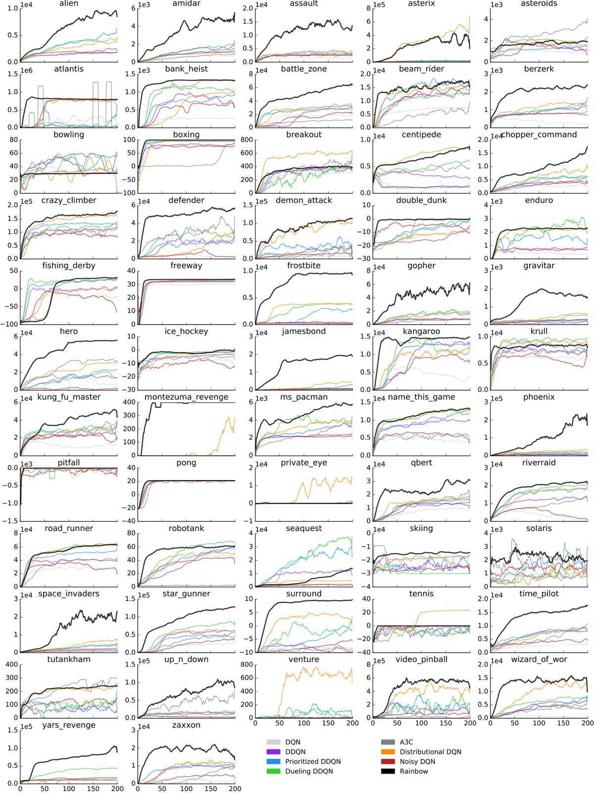
Figure 5: Learning curves for Rainbow and the baselines discussed in the paper, for each individual game. Every curve is smoothed with a moving average of 10 to improve readability.

图 5：论文讨论的 Rainbow 与基线在各单独游戏上的学习曲线。每条曲线用窗口为 10 的滑动平均平滑，以提高可读性。

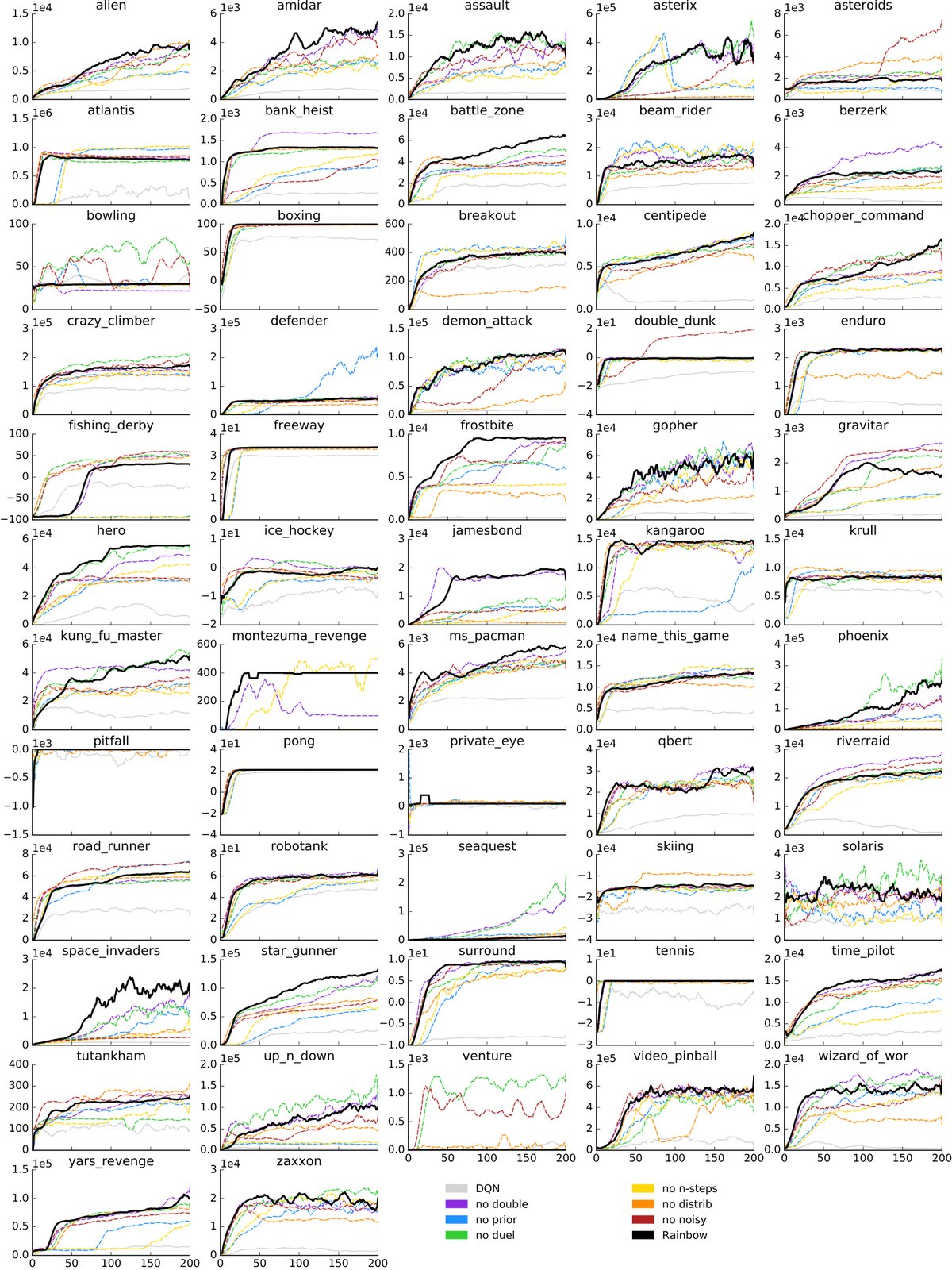
Figure 6: Learning curves for Rainbow and its ablations, for each individual game. Every curve is smoothed with a moving average of 10 to improve readability.

图 6：Rainbow 与其消融在各单独游戏上的学习曲线。每条曲线用窗口为 10 的滑动平均平滑，以提高可读性。

2017

[2013] Bellemare, M. G.; Naddaf, Y.; Veness, J.; and Bowling, M. 2013. The arcade learning environment: An evaluation platform for general agents. J. Artif. Intell. Res. (JAIR) 47:253–279.

[2016] Bellemare, M. G.; Srinivasan, S.; Ostrovski, G.; Schaul, T.; Saxton, D.; and Munos, R. 2016. Unifying count-based exploration and intrinsic motivation. In NIPS .

[2017] Bellemare, M. G.; Dabney, W.; and Munos, R. 2017. A distributional perspective on reinforcement learning. In ICML .

[2016] Blundell, C.; Uria, B.; Pritzel, A.; Li, Y.; Ruderman, A.; Leibo, J. Z.; Rae, J.; Wierstra, D.; and Hassabis, D. 2016. Model-Free Episodic Control. ArXiv e-prints .

[2016] Dosovitskiy, A., and Koltun, V. 2016. Learning to act by predicting the future. CoRR abs/1611.01779.

[2017] Fortunato, M.; Azar, M. G.; Piot, B.; Menick, J.; Osband, I.; Graves, A.; Mnih, V.; Munos, R.; Hassabis, D.; Pietquin, O.; Blundell, C.; and Legg, S. 2017. Noisy networks for exploration. CoRR abs/1706.10295.

[2015] Hausknecht, M., and Stone, P. 2015. Deep recurrent Q-learning for partially observable MDPs. arXiv preprint arXiv:1507.06527 .

[2016] He, F. S.; Liu, Y.; Schwing, A. G.; and Peng, J. 2016. Learning to play in a day: Faster deep reinforcement learning by optimality tightening. CoRR abs/1611.01606.

[2016] Jaderberg, M.; Mnih, V.; Czarnecki, W. M.; Schaul, T.; Leibo, J. Z.; Silver, D.; and Kavukcuoglu, K. 2016. Reinforcement learning with unsupervised auxiliary tasks. CoRR abs/1611.05397.

[2014] Kingma, D. P., and Ba, J. 2014. Adam: A method for stochastic optimization. In Proceedings of the 3rd International Conference on Learning Representations (ICLR) .

[2016a] Kulkarni, T. D.; Narasimhan, K.; Saeedi, A.; and Tenenbaum, J. B. 2016a. Hierarchical deep reinforcement learning: Integrating temporal abstraction and intrinsic motivation. CoRR abs/1604.06057.

[2016b] Kulkarni, T. D.; Saeedi, A.; Gautam, S.; and Gershman, S. J. 2016b. Deep successor reinforcement learning. arXiv preprint arXiv:1606.02396 .

[1992] Lin, L.-J. 1992. Self-improving reactive agents based on reinforcement learning, planning and teaching. Machine Learning 8(3):293–321.

[2013] Mnih, V.; Kavukcuoglu, K.; Silver, D.; Graves, A.; Antonoglou, I.; Wierstra, D.; and Riedmiller, M. A. 2013. Playing atari with deep reinforcement learning. CoRR abs/1312.5602.

[2015] Mnih, V.; Kavukcuoglu, K.; Silver, D.; Rusu, A. A.; Veness, J.; Bellemare, M. G.; Graves, A.; Riedmiller, M.; Fidjeland, A. K.; Ostrovski, G.; Petersen, S.; Beattie, C.; Sadik, A.; Antonoglou, I.; King, H.; Kumaran, D.; Wierstra, D.; Legg, S.; and Hassabis, D. 2015. Human-level control through deep reinforcement learning. Nature 518(7540):529–533.

[2016] Mnih, V.; Badia, A. P.; Mirza, M.; Graves, A.; Lillicrap, T.; Harley, T.; Silver, D.; and Kavukcuoglu, K. 2016. Asynchronous methods for deep reinforcement learning. In International Conference on Machine Learning .

[2015] Nair, A.; Srinivasan, P.; Blackwell, S.; Alcicek, C.; Fearon, R.; De Maria, A.; Panneershelvam, V.; Suleyman, M.; Beattie, C.; Petersen, S.; Legg, S.; Mnih, V.; Kavukcuoglu, K.; and Silver, D. 2015. Massively parallel methods for deep reinforcement learning. arXiv preprint arXiv:1507.04296 .

[2016] O’Donoghue, B.; Munos, R.; Kavukcuoglu, K.; and Mnih, V. 2016. Pgq: Combining policy gradient and q-learning. CoRR abs/1611.01626.

[2016] Osband, I.; Blundell, C.; Pritzel, A.; and Roy, B. V. 2016. Deep exploration via bootstrapped dqn. In NIPS .

[2017] Salimans, T.; Ho, J.; Chen, X.; and Sutskever, I. 2017. Evolution strategies as a scalable alternative to reinforcement learning. CoRR abs/1703.03864.

[2015] Schaul, T.; Quan, J.; Antonoglou, I.; and Silver, D. 2015. Prioritized experience replay. In Proc. of ICLR .

[2015] Schulman, J.; Levine, S.; Moritz, P.; Jordan, M.; and Abbeel, P. 2015. Trust region policy optimization. In Proceedings of the 32Nd International Conference on International Conference on Machine Learning - Volume 37 , ICML’15, 1889–1897. JMLR.org.

[2017] Sharma, S.; Lakshminarayanan, A. S.; and Ravindran, B. 2017. Learning to repeat: Fine grained action repetition for deep reinforcement learning. arXiv preprint arXiv:1702.06054 .

[2015] Stadie, B. C.; Levine, S.; and Abbeel, P. 2015. Incentivizing exploration in reinforcement learning with deep predictive models. CoRR abs/1507.00814.

[1998] Sutton, R. S., and Barto, A. G. 1998. Reinforcement Learning: An Introduction . The MIT press, Cambridge MA.

[1988] Sutton, R. S. 1988. Learning to predict by the methods of temporal differences. Machine learning 3(1):9–44.

[2012] Tieleman, T., and Hinton, G. 2012. Lecture 6.5-rmsprop: Divide the gradient by a running average of its recent magnitude. COURSERA: Neural networks for machine learning 4(2):26–31.

[2016] van Hasselt, H.; Guez, A.; Guez, A.; Hessel, M.; Mnih, V.; and Silver, D. 2016. Learning values across many orders of magnitude. In Advances in Neural Information Processing Systems 29 , 4287–4295.

[2016] van Hasselt, H.; Guez, A.; and Silver, D. 2016. Deep reinforcement learning with double Q-learning. In Proc. of AAAI , 2094–2100.

[2010] van Hasselt, H. 2010. Double Q-learning. In Advances in Neural Information Processing Systems 23 , 2613–2621.

[2017] Vezhnevets, A. S.; Osindero, S.; Schaul, T.; Heess, N.; Jaderberg, M.; Silver, D.; and Kavukcuoglu, K. 2017. Feudal networks for hierarchical reinforcement learning. CoRR abs/1703.01161.

[2016] Wang, Z.; Schaul, T.; Hessel, M.; van Hasselt, H.; Lanctot, M.; and de Freitas, N. 2016. Dueling network architectures for deep reinforcement learning. In Proceedings of The 33rd International Conference on Machine Learning , 1995–2003.