用大模型搜量子电路:七项任务同时压低 Toffoli 与比特数
Discovering state-of-the-art quantum circuits with large language models
用大语言模型发现先进量子电路(Discovering state-of-the-art quantum circuits with large language models)
Andi Gu Email: andigu@g.harvard.edu Affiliation: Harvard Quantum Initiative for Science and Engineering, Cambridge, MA 02138, USA Affiliation: Department of Physics, Harvard University, Cambridge, MA 02138, USA Affiliation: Anthropic STEM Fellows Program Alek H. Kemeny Affiliation: Anthropic Susanne F. Yelin Affiliation: Harvard Quantum Initiative for Science and Engineering, Cambridge, MA 02138, USA Affiliation: Department of Physics, Harvard University, Cambridge, MA 02138, USA Mikhail D. Lukin Affiliation: Harvard Quantum Initiative for Science and Engineering, Cambridge, MA 02138, USA Affiliation: Department of Physics, Harvard University, Cambridge, MA 02138, USA Affiliation: QuEra Computing, 1380 Soldiers Field Road, Boston, MA 02135, USA
Abstract
摘要
Significant efforts are currently being directed toward the implementation of large-scale quantum information processors, but realizing useful quantum advantage also requires the development of efficient quantum algorithms. While for many practical problems the dominant resource costs are associated with a small set of computational primitives, optimizing them in the quantum setting presents unique challenges, including a reversibility constraint absent from ordinary classical computation. Here we introduce an evolutionary framework in which large language models (LLMs) propose circuit designs and an independent evaluator verifies and scores them. We apply this framework to tasks spanning numerical computation, chemistry, optimization, quantum simulation, and number theory. In seven of the eight tasks, the discovered circuits significantly reduce both Toffoli and qubit counts relative to the state of the art. In the eighth, the search discovers a new reversible architecture for prime-field modular inversion. By handling reversibility differently, the architecture makes divsteps—a classical algorithm previously impractical for reversible integer arithmetic—viable and substantially improves the Toffoli–qubit trade-off for modular inversion. These results open the door for evaluator-guided LLM co-design of new algorithmic structures for quantum computation.
大规模量子信息处理器的实现正投入大量努力,但实现有用的量子优势还需要高效量子算法。对许多实际问题,主导资源成本集中在少数计算原语上,而在量子设定下优化它们面临独特挑战,包括普通经典计算所没有的可逆性约束。本文提出进化框架:大语言模型(LLM)提议电路设计,独立评估器验证并打分。我们将其应用于跨越数值计算、化学、优化、量子模拟与数论的任务。八项任务中七项,发现的电路相对当时最优显著同时降低 Toffoli 数与量子比特数。第八项中,搜索发现素数域模逆的新可逆架构。通过不同方式处理可逆性,该架构使 divsteps——一种先前对可逆整数算术不实用的经典算法——变得可行,并显著改善模逆的 Toffoli–量子比特权衡。这些结果为评估器引导的 LLM 协同设计量子计算新算法结构打开大门。
Computational primitives based on classical function evaluation play a central role in a wide range of quantum algorithms. Such primitives include decoding routines for optimization [1], numerical functions for quantum simulation [2], arithmetic routines for number theory [3], and quantum read-only memory (QROM), which coherently loads classically specified data into quantum registers [4]. To operate on quantum data, these functions must be compiled into circuits that can be executed coherently on quantum hardware. This imposes two constraints absent from ordinary classical programs. First, because the input may be in superposition, the circuit cannot inspect an intermediate value and select an ordinary classical control-flow path. Data-dependent behavior is instead expressed through controlled operations within a fixed gate sequence, so every branch contributes to the circuit’s cost even if it applies only to some inputs. Second, the computation must be reversible: intermediate information cannot simply be overwritten or discarded. Temporary values must eventually be uncomputed, returning their qubits to their initial state and preventing residual information from remaining entangled with the output. Until they are uncomputed, these values occupy additional qubits. At the same time, when bounded error is permitted, machinery needed only for rare or atypical inputs can sometimes be omitted, reducing resource requirements while keeping the failure probability controlled. Efficient coherent compilation is of major practical importance, and recent reductions in resource requirements have come from coordinated changes to arithmetic algorithms, data representations, and their reversible implementation [5, 6]. Such redesigns are difficult for general quantum circuits because directly testing correctness can require exponentially expensive classical simulation or fully operational large-scale quantum processors. Automated circuit optimizers therefore typically preserve correctness by restricting the search to predefined equivalence-preserving rewrites [7], limiting them to variations of a fixed design.
基于经典函数求值的计算原语在广泛量子算法中起核心作用,包括优化中的译码例程 [1]、量子模拟中的数值函数 [2]、数论中的算术例程 [3],以及把经典指定数据相干装入量子寄存器的量子只读存储器(QROM) [4]。要作用于量子数据,这些函数必须编译成可在量子硬件上相干执行的电路。这施加了普通经典程序没有的两条约束。其一,输入可能处于叠加,电路不能检查中间值再选择普通经典控制流;数据依赖行为须通过固定门序列内的受控运算表达,因此每个分支都计入电路成本,即使只对部分输入生效。其二,计算必须可逆:中间信息不能简单覆盖或丢弃;临时值最终须反计算,使量子比特回到初态,并防止残留信息与输出纠缠。在反计算之前,这些值占用额外量子比特。同时,在允许有界误差时,仅服务于稀有或非典型输入的机制有时可省略,从而在控制失败概率的前提下降低资源需求。高效相干编译具有重大实践意义;近期资源下降往往来自算术算法、数据表示及其可逆实现的协同改动 [5, 6]。对一般量子电路,此类重设计困难,因为直接测正确性可能需要指数代价的经典模拟或已运行的大规模量子处理器。自动电路优化器因此通常把搜索限制在预定义的保等价改写 [7],从而只能得到固定设计的变体。
Here we introduce a framework that pairs large language model (LLM) proposals with an independent evaluator that verifies and scores each candidate. We focus on a class of quantum circuits that compute a classical function : for an arbitrary input , the circuit must act as , where and are computational-basis states of the input and output registers, respectively. By linearity, this coherent action is correct if the circuit performs the required map on every computational-basis input: . This basis-state reduction makes candidate circuits amenable to programmatic evaluation, since every allowed operation maps a computational-basis state to another computational-basis state, possibly changing its phase, but never creating a superposition [8]. The action of a candidate on any chosen input can therefore be simulated by tracking a bit string and its phase, rather than amplitudes. Resource accounting is also simple: we use the Toffoli count and the peak qubit count , and rank circuits by their product, the -cost. Together, these properties let us build an efficient, programmatic evaluator that checks the correctness and resource cost of any candidate circuit design.
我们提出将大语言模型(LLM)提案与独立评估器配对的框架:评估器验证并给每个候选打分。关注计算经典函数 的一类量子电路:对任意输入 ,电路须实现 ,其中 、 分别为输入与输出寄存器的计算基态。由线性性,该相干作用正确当且仅当电路对每个计算基输入执行所需映射:。这一基态归约使候选电路可用程序化评估,因为每个允许运算把计算基态映到计算基态,可改相位但从不制造叠加 [8]。因此候选对任一选定输入的作用可通过跟踪比特串及其相位模拟,而非 振幅。资源核算也简单:用 Toffoli 数 与峰值量子比特数 ,按乘积 成本排序。这些性质合起来让我们构建高效、可编程的评估器,检查任一候选电路设计的正确性与资源成本。
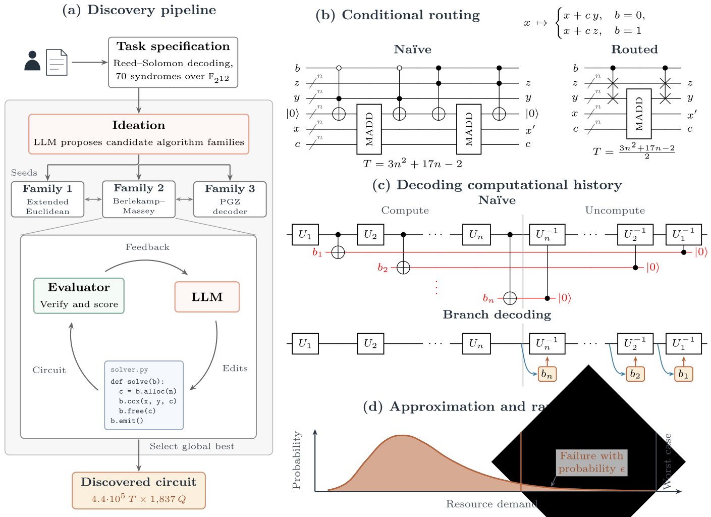
Figure 1: Overview of the circuit-discovery framework. (a) A hand-written task specification defines the circuit design task (for example, Reed–Solomon decoding) and is given to an LLM. The LLM proposes architecturally different approaches (algorithm families; here extended Euclidean, Berlekamp–Massey, and Peterson–Gorenstein–Zierler (PGZ) decoders), which are then developed and optimized in parallel. Strong candidates are periodically shared between families to allow for cross-pollination of useful ideas. (b) Conditional routing reduces the cost of coherent control flow: for instance, two controlled multiply-adds (MADDs) become inexpensive controlled swaps and one shared arithmetic block. (c) Branch decisions that a naïve reversible computation stores during the forward pass (red) can instead be decoded from the current state during uncomputation. (d) When an application permits bounded error, allowing rare failures on atypical, costly inputs reduces resource requirements.
图 1:电路发现框架概览。(a) 手写任务规格定义电路设计任务(例如 Reed–Solomon 译码)并交给 LLM。LLM 提出架构不同的路径(算法族;此处为扩展欧几里得、Berlekamp–Massey 与 Peterson–Gorenstein–Zierler (PGZ) 译码器),再并行发展与优化。强候选定期在族间共享,以便有用思想交叉授粉。(b) 条件路由降低相干控制流成本:例如两个受控乘加(MADD)变成便宜的受控交换与一个共享算术块。(c) 朴素可逆计算在正向过程存储的分支决策(红)可改为在反计算时从当前状态译出。(d) 当应用允许有界误差时,允许对非典型、昂贵输入的稀有失败可降低资源需求。
Each search begins from a hand-written task specification and a blank program; the specification states the required circuit behavior but provides no implementation guidance. The LLM proposes a candidate and iteratively revises it using evaluator feedback (Figure 1(a)). Previous work represents candidates as sequences of gates or predefined circuit blocks [9, 10], which can obscure the algorithmic structure of the circuit. Our framework instead lets the LLM propose and revise candidates through a high-level Python interface, where reusable functions and ordinary programming constructs make that structure explicit. This allows a single conceptual change to reorganize operations throughout the circuit, while the evaluator tests its consequences for correctness and resource cost. However, purely iterative refinement of a single candidate can remain tied to the architecture from which it began, resulting in convergence to local (but not necessarily global) optima. We therefore start with an ideation stage in which the LLM is prompted to propose several distinct algorithm families, each representing a different approach to the problem. Circuits within each family are optimized independently in parallel, allowing the search to explore different strategies rather than only variations of one design. Well-performing candidates are periodically shared between families so that an idea discovered in one approach can inform another.
每次搜索从手写任务规格与空白程序开始;规格陈述所需电路行为但不给实现指导。LLM 提出候选并用评估器反馈迭代修订(图 1(a))。先前工作把候选表示为门序列或预定义电路块 [9, 10],可能掩盖电路的算法结构。我们的框架让 LLM 经高层 Python 接口提案与修订,可复用函数与普通编程构造使结构显式。于是单一概念改动可重组整条电路的运算,评估器则检验其对正确性与资源成本的后果。然而纯迭代 refinement 单个候选可能束缚于起步架构,收敛到局部(未必全局)最优。因此我们先做构思阶段:提示 LLM 提出若干不同的算法族,各自代表不同解题路径。各族电路独立并行优化,使搜索探索不同策略而非单一设计的变体。表现好的候选定期跨族共享,使一族发现的思想可启发另一族。
Across eight diverse compilation tasks, the discovered circuits repeatedly exhibit three common principles of algorithm–circuit co-design. These principles address the features of coherent compilation described above: expressing data-dependent control flow, making intermediate computations reversible without retaining their entire history, and using a failure budget to remove circuit resources devoted to atypical cases (see Figure 1).
在八项多样编译任务上,发现的电路反复呈现算法—电路协同设计的三条共同原则。这些原则针对上文相干编译特征:表达数据依赖控制流、在不保留全部历史的前提下使中间计算可逆,以及用失败预算移除专用于非典型情形的电路资源(见图 1)。
Design principles
设计原则
One recurring principle in the circuits discovered by the search is to replace conditional arithmetic with conditional routing. A naïve coherent translation of a casewise classical algorithm includes a separately controlled arithmetic block for every branch. The discovered circuits instead use a representation in which the branches differ primarily in which values occupy particular computational roles. Relatively cheap controlled swaps then route the appropriate values into those roles, one unconditional arithmetic path performs the expensive work, and further routing places the results in their required registers. In this sense, where a classical program routes execution to the selected operation, the coherent circuit routes the selected data through a shared operation. The idea resembles bucket-brigade quantum random-access memory (QRAM) [11].
搜索发现的电路中一条反复出现的原则是用条件路由替代条件算术。朴素地把分情形经典算法相干翻译,会为每个分支包含单独受控的算术块。发现的电路改用一种表示:分支差异主要在于哪些值占据特定计算角色。相对便宜的受控交换把适当值路由进这些角色,一条无条件算术路径完成昂贵工作,再进一步路由把结果放到所需寄存器。在此意义上,经典程序把执行路由到所选操作,相干电路则把所选数据路由过共享操作。这一想法类似桶旅量子随机访问存储器(QRAM) [11]。
For example, consider four -qubit fixed-point registers , , , and , together with a control qubit . Suppose that we wish to perform
例如,考虑4个-quit固定点登记册 ,,和,以及一个控制quit . 假设我们想表演
$$x\longmapsto\begin{cases}x+cy&\text{for }b=0,\
x+cz&\text{for }b=1,\end{cases} \tag{1}$$
while returning , , and unchanged. A naïve implementation uses two controlled multiply-adds. Conditional routing instead swaps and according to , applies one uncontrolled multiply-add, and undoes the swap. For the standard schoolbook construction [12], this reduces the Toffoli count from to , as shown in Figure 1(b).
同时使 、、 不变。朴素实现使用两次受控乘加。条件路由则按 交换 与 ,施加一次不受控乘加,再撤销交换。对标准课本构造 [12],这把 Toffoli 数从 降到 ,如图 1(b)。
More generally, conditional routing requires canonicalizing branch-dependent states into a representation on which the same expensive computation applies. Schematically, when the branch can be expressed as , the circuit need only control the inexpensive routing transformation ; the expensive kernel appears once and need not be controlled. Finding such a decomposition typically takes more than recognizing identical arithmetic in two branches: it exploits an equivalence in the required output so that apparently different updates become instances of the same computation. The difficulty lies less in the routing circuit than in determining which branch-dependent differences matter and which can be absorbed into a shared representation.
更一般地,条件路由要求把分支依赖状态规范化为同一昂贵计算适用的表示。示意上,当分支可写成 时,电路只需控制便宜的路由变换 ;昂贵内核 出现一次且不必受控。找到这种分解通常不只是认出两分支中相同算术:它利用所需输出上的等价,使表面上不同的更新成为同一计算的实例。难点较少在路由电路本身,而在判定哪些分支依赖差异要紧、哪些可吸收进共享表示。
Reversibility creates a second challenge: reversing a conditional update requires knowing which branch was taken during the forward computation. A naïve implementation records each decision in a history stack whose size grows with the number of updates. But the branch decisions need not always be stored explicitly: different branches may leave distinguishable patterns in registers that remain available during uncomputation. As illustrated in Figure 1(c), the circuit can recover the branch bit from such a pattern, use it to select the appropriate inverse update, and then clear the recovered bit, so the register contents serve as an inexpensive record of the branch decisions. For example, suppose we have a register that begins at . In round , conditioned on some branch bit , we add , so that
可逆转性产生了第二个挑战:要逆转有条件的更新,需要知道在前期计算中采取了哪个分支. 一个天真的执行记录每个决定在一个历史堆栈中,其规模随着更新次数的增加而增加。 但是,分支机构的决定并不总是明确保存:不同的分支机构可能会在登记册中留下在不计算期间仍然可用的可区分的模式。 如图1(c)所示,电路可以从这种模式中回收分支位,使用它来选择适当的反向更新,然后清除回收位,因此寄存器内容充当分支决定的廉价记录. 例如,假设我们有一个始于的登记簿。 在回合中,以某些分支位值为条件,我们增加了,这样,
For arbitrary values of , there is no way to tell from which branch was taken. Globally, however, there is an important invariant: , and therefore bit of must equal . During uncomputation, the circuit can simply read this bit to recover . The computation’s evolving state thus supplies the branch decisions in reverse order without a separate history stack. In general, finding such a decoder requires the forward algorithm, its data representation, and its uncomputation procedure to be designed together. Viewed locally, an update may be ambiguous, since either branch can appear to admit a valid predecessor. The ambiguity can disappear once the circuit is restricted to states reachable from the prescribed initialization, where a relation across the registers can distinguish histories that no single register can.
对于的任意值,无法从中分出哪个分支. 你说什么? 但是,在全球范围内,有一种重要的变异:,因此,的bit 必须等于. 在不计算时,电路可以简单地读取这个位点以恢复. 因此,计算正在演变的状态以反向顺序提供分支决定,而不另设历史堆栈。 一般来说,找到这样的解码器需要前方算法,其数据表示,及其不计算程序一起设计. 从本地角度看,更新可能含糊不清,因为任何一个分支似乎都承认有效的前身。 一旦电路被限制在从规定的初始化可达到的状态上,那么模糊性就可能消失,在这种状态下,登记册之间的一种关系可以区分任何单一登记册都无法区分的历史。
The third principle exploits the small but finite failure probability permitted by most quantum algorithms. Turning this failure budget into resource savings, however, is not automatic. One must first identify the rare inputs that determine worst-case resource requirements. Unlike a classical program, a quantum circuit must contain the gates and ancillas required by every supported path. A rare input can therefore determine the circuit’s Toffoli count or peak qubit count. Yet identifying such inputs is not enough: the circuitry supporting them may not be separable from the computation on typical inputs. The co-design task is to reorganize the computation so that the additional resources required by rare inputs are localized—for example, to extra iterations, stack entries, or arithmetic lanes. Those components can then be omitted while confining failure to the low-probability inputs that require them (Figure 1(d)). In what follows we show how these design principles result in significantly improved algorithmic circuits across a wide variety of quantum tasks.
第三项原则利用大多数量子算法允许的微小但有限的故障概率. 然而,将这一失败的预算转化为资源节约并不是自动的。 必须首先确定决定最坏情况所需资源的稀有投入。 与古典程序不同,量子电路必须包含每个支持路径所需的门和角. 因此,一个罕见的输入可以决定电路的Toffoli计数或峰值qubit计数. 然而,确定这种投入是不够的:支持这种投入的电路可能无法与典型投入的计算分开。 共同设计的任务是重组计算,以便稀有输入所需的额外资源能够本地化——例如,用于额外迭代、堆栈条目或算术道。 然后可以省略这些组件,同时将失败限制在需要的低概率输入(图1(d))。 接下来,我们展示这些设计原理如何 使算法电路大大改进 跨越各种各样的量子任务。
Reversible syndrome decoding for DQI
面向 DQI 的可逆伴随式译码
Decoded quantum interferometry (DQI) is a quantum algorithm that turns certain optimization problems into decoding problems for classical error-correcting codes, using quantum interference to favor better solutions. A central application is optimal polynomial intersection (OPI), a form of polynomial fitting over finite fields for which DQI offers a superpolynomial speedup over known classical algorithms. DQI achieves this by using a Reed–Solomon decoder as a subroutine within the quantum computation [1]. The decoder identifies the positions and values of errors from a collection of algebraic checks called syndromes. DQI requires this decoding to run coherently on a superposition of inputs, making the reversible decoder a dominant resource cost. [13] compiled DQI circuits for OPI over binary extension fields using reversible Reed–Solomon decoders based on the extended Euclidean algorithm.
译码量子干涉(DQI)是一种量子算法,把某些优化问题变成经典纠错码的译码问题,用量子干涉偏好更好解。核心应用之一是最优多项式交(OPI)——有限域上的一类多项式拟合,DQI 相对已知经典算法提供超多项式加速。DQI 通过在量子计算内把 Reed–Solomon 译码器当子程序实现这一点 [1]。译码器从称为伴随式的代数校验集合识别错误位置与值。DQI 要求该译码在输入叠加上相干运行,使可逆译码器成为主导资源成本。[13] 用基于扩展欧几里得算法的可逆 Reed–Solomon 译码器,为二元扩域上的 OPI 编译了 DQI 电路。
We study their primary Reed–Solomon instance, in which 70 syndrome values uniquely determine an error pattern containing at most 35 errors. Our search framework discovered a circuit that replaces their synchronized Euclidean solve with the Berlekamp–Massey (BM) recurrence. BM substantially reduces the arithmetic cost, but its updates overwrite intermediate values that a naïve reversible implementation would retain in a large history stack. The discovered circuit preserves BM’s arithmetic advantage while avoiding most of this storage (Figure 2).
我们研究其主要 Reed–Solomon 实例:70 个伴随式值唯一确定至多含 35 个错误的错误模式。我们的搜索框架发现的电路用 Berlekamp–Massey(BM)递推替换其同步欧几里得求解。BM 大幅降低算术成本,但其更新会覆盖中间值,朴素可逆实现须把它们保留在大历史栈中。发现的电路在保留 BM 算术优势的同时避免了大部分这类存储(图 2)。
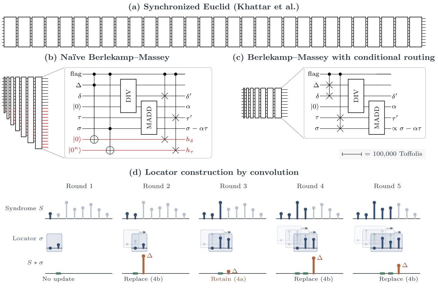
Figure 2: Reversible Reed–Solomon decoding. (a) The synchronized extended-Euclidean construction of [13] requires approximately million Toffolis for the locator solve. (b) Berlekamp–Massey reduces this cost to approximately Toffolis but naïvely accumulates intermediate information (red). DIV forms , MADD applies the multiply-add, and the flag marks the replace case. (c) Conditional routing preserves this arithmetic advantage while avoiding most history storage. Block widths are proportional to Toffoli count. (d) Locator construction as convolution with the syndrome sequence. The discrepancy is the convolution at the next syndrome; a nonzero value requires updating the locator.
图2:Reversible Reed – Solomon解码. (a)同步扩展-Euclidean 构造 [13] 需要大约万Toffoli用于定位解析. (b) Berlekamp - 梅西将这一成本降低到大约 Toffolis,但天真地积累中间信息(红色). DIV形式为 ,MADD应用乘法加法,旗标为替换大小写. (c) 有条件的路由保持这种算术优势,同时避免大多数历史存储。 块宽度与Toffoli计数成正比. (d) 定位器构造与综合症序列结合。 偏差是下一个综合征的演化;非零值需要更新定位器.
Reed–Solomon decoding amounts to determining which positions in the data contain errors. The error positions are encoded in a locator polynomial , whose roots identify those positions. To recover the locator coefficients, BM solves for the lowest-degree nonzero polynomial whose convolution (see Figure 2(d)) with the syndrome sequence vanishes:
Reed–Solomon解码等于确定数据中哪些位置含有错误. 错误位置被编码在一个定位器多号中,其根部识别这些位置. 为了恢复定位系数,BM解决了与综合征序列发生共化(见图2(d))而消失的低度非零倍数:
BM constructs the locator incrementally. At each round, the convolution evaluated at the next syndrome gives the discrepancy : if it vanishes, no correction is needed; otherwise, BM adjusts the locator coefficients and, when necessary, increases its degree.
BM逐渐构建定位器. 在每一回合,在下一轮综合征中评估的演化值给出了差异:如果消失,不需要纠正;否则,BM会调整定位系数,并在必要时提高其程度.
To make a correction without invalidating previous rounds of updates, BM retains an earlier polynomial as a correction template, together with its nonzero discrepancy . When , BM scales by and applies the correction . BM keeps the template until the current locator has accumulated enough information from subsequent syndromes to take over its role:
为了在不否定前几轮更新的情况下作出更正,BM保留了较早的多元作为校正模板,同时保留其非零差异. 当时,BM以表示比例,并应用的校正. BM保留模板,直到当前定位器从后续综合征中积累足够的信息来接管其角色:
The replace update in Equation 4b creates the main reversibility problem: it overwrites the previous template and discrepancy . A naïve reversible implementation stores these displaced values so that the update can later be undone. Over repeated rounds, this accumulates a history of whole polynomials (Figure 2(b)).
Equation 4b中的替换更新产生了主要的可逆性问题:它覆盖了先前的模板,与存在差异. 可逆的天真执行储存了这些被置换的价值观,以便日后可以取消更新。 在反复的回合中,它积累了整个多名体的历史(图2(b))。
The discovered circuit avoids this polynomial history by exploiting a freedom in the decoding task: the locator is needed only up to a nonzero multiplicative factor, because rescaling leaves its roots unchanged. The circuit (Figure 2(c)) therefore implements a rescaled version of both branches of Equation 4, using simple conditional routing and a single shared update:
发现的电路通过在解码任务中利用自由来避免这种多名历史:定位器仅需要达到非零倍增因子,因为再缩放使其根基不变. 因此,电路(图2(c))采用简单的有条件路由和单一共享更新,对方程式4的两分支执行一个重级版本:
The result differs from the locator in the unrescaled update only by the nonzero scale factor and so has the same roots. Both branches can then use one shared arithmetic path without storing the displaced template .
结果与未调整更新中的定位器不同,只有非零尺度系数,因此也有相同的根. 两个分支然后可以使用一个共享的算术路径,而无需存储被忽略的模板 .
This resolves the history problem for the polynomial registers, but the discrepancies present a second reversibility problem. To uncompute a correction, the circuit must recover whichever discrepancy is no longer present after the update. The replace case of Equation 5b overwrites the stored value with , but the circuit can decode from the constant coefficients of the updated locator registers. BM shifts the template by one power of every round, so has zero constant coefficient entering the round. Writing and for the constant coefficients after the update gives . This case thus adds no entry to the history stack. In fact, the circuit never stores at all: the same relation fixes in terms of the locator’s constant coefficient (Supplementary Information [SI] I.1). The retain update of Equation 5a is the exception: it keeps the previous discrepancy , while the current discrepancy , which is needed to reverse the correction, remains only in a temporary register. Each retain update therefore stores on the history stack. In the worst case, 35 stack entries (665 qubits) would be needed. Under the DQI input distribution, a second stack entry is required with probability , so the discovered circuit allocates only one stack entry (19 qubits instead of 665) and permits failure on these rare inputs.
这解决了多名登记簿的历史问题,但差异提出了第二个可逆转性问题。 为了校正,电路必须收回更新后已不存在的差额。 方程式5b的替换例将存储值XX 是不是 覆盖为 ,但电路可以从更新的定位器登记册的恒定系数中解码 * . BM每回合以一个功率的改变模板,因此进入回合的恒系数为0. 在更新后为恒系数写入和给出 . 因此,本案没有增加历史堆栈条目。 事实上,电路从不存储:同一关系用定位器的常数(补充信息[SI]I.1)来固定. 保留更新的方程式5a是例外:它保留了先前的差异,而目前的差异是逆转校正所需的,它只保留在一个临时登记册中. 因此,每个系统都保留更新,将存储在历史堆栈上。 在最坏的情况下,需要35个堆栈条目(665个qubits). 在DQI输入分布下,需要用概率为的第二个堆栈条目,因此发现的电路只分配一个堆栈条目(19个qubit而不是665个),并允许这些稀有输入失败.
Together, these transformations make the arithmetically efficient BM algorithm suitable for reversible computation.
这些转变加在一起,使得算术效率的BM算法适合可逆计算.
Reversible modular inversion
可逆模逆
Modular inversion is the task of finding such that , given a nonzero input and a prime . It is a central arithmetic subroutine in a range of quantum algorithms [14, 3]. A standard way to compute the inverse is through the extended Euclidean algorithm. Euclidean algorithms repeatedly simplify a pair of integers while preserving their greatest common divisor. By tracking how this divisor is expressed in terms of the original inputs, they also recover coefficients satisfying , so is the inverse of modulo .
模态反转是找到的任务,这样,得到非零输入的和质值的. 它是一系列量子算法[14,3]中的中央算术子例程. 计算反向的一个标准方法是通过延伸的欧几利得算法. 欧几利得算法在保留其最大的常见二维器的同时,反复简化一对整数. 通过跟踪这种divisor是如何用原始输入表达的,它们也回收了满足的系数,因此是 modulo 的逆差.
Divsteps is a variant of the Euclidean algorithm that replaces division with conditional additions, subtractions, and halving [15]. Starting from and , the goal is to reduce the pair to and while preserving their greatest common divisor. The basic strategy is to hold the odd integer fixed while reducing : if is even, it can be halved directly; if is odd, adding or subtracting first makes it even. These operations preserve the greatest common divisor because is odd. Holding fixed indefinitely, however, would leave only one integer being reduced, so the algorithm must periodically swap their roles. A small signed counter schedules these swaps without ever comparing and : it roughly tracks how many more bits has than , so a swap occurs once is likely the smaller of the two. This allows both integers to be reduced using only inexpensive arithmetic and control. Two auxiliary integers and track the input’s contribution in a scaled form: after steps, they satisfy and . Thus, at termination, gives the desired inverse up to the scaling factor . The scaling keeps the coefficient updates free of division. Starting from , each step applies one of three updates:
divsteps)是欧几利得算法的一个变种,它用有条件的加法,减法,并减半[15]. 从和开始,目标是在保留它们最大的共同分光器的同时,将对子减为和. 基本策略是将奇数整数固定在减少的同时:如果是均匀的,可以直接将它减半;如果是奇数,则增减首先使其均匀. 由于是奇数,这些操作保留了最大的常见的二极管. 然而,无限期地持有将只减少一个整数,因此算法必须定期互换角色. 一个小型的签名计数器列表 这些互换从未比较过和:它大致跟踪了有多少比更多的位数,所以一旦很可能是两者中较小的位数,就发生了互换. 这使得只使用廉价的算术和控制就可以减少两个整数。 两个辅助整数和以缩放的形式跟踪输入的贡献:在步骤之后,它们满足和. 因此,在终止时,给出了期望的逆比值,达到。 缩放使系数更新不受分割。 从开始,每个步骤适用三个更新中的一个:
Classically, each update overwrites the current state. Reversing the computation, however, requires knowing which of the three updates was applied. A naïve implementation would store this choice at every step, accumulating a history stack alongside the arithmetic registers. The discovered circuit instead recovers decisions from the current arithmetic state. Some decisions are easy to recover from the updated registers, while others require a more involved decoding procedure. We label each update by two bits: records whether the step swaps the roles of and , and records whether the incoming is odd. The updates in Equations 6a, 6b and 6c have labels , respectively. The task during uncomputation is to recover these bits from the updated state.
经典中,每次更新都会覆盖当前状态. 但是,要推翻计算,就需要知道三个更新中哪一个已经适用。 一个天真的执行将把这种选择储存在每一个步骤上,在算术登记册旁边积累一个历史堆。 所发现的电路转而从目前的算术状态中恢复决定. 有些决定很容易从更新的登记册中收回,而另一些决定则需要更多的解码程序。 我们给每个更新贴上两个比特的标签:记录步骤是否互换和的角色,记录进球的是否是奇数. 第6a、6b和6c条的更新分别有的标签。 未计算期间的任务是从更新状态中回收这些位.
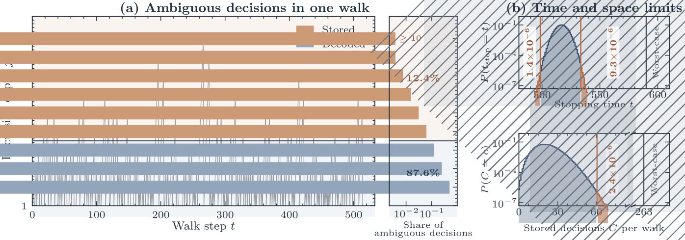
Figure 3: Making divsteps reversible with minimal overhead. (a) Excursion depth in one representative walk. Dots mark ambiguous decisions. We use a cutoff , so all ambiguous decisions with are stored rather than decoded. The histogram shows the distribution of excursion depths over uniformly sampled walks: only 12.4% of ambiguous decisions reach . (b) Empirical stopping-time and history-size distributions. The discovered circuit assumes that every walk terminates between steps and ; this assumption fails with probability . It also allocates enough qubits to store at most 60 branch decisions, which is sufficient for all but a fraction of walks.
图3:使潜水器可逆性最小,但间接费用最低。 点点标志着模棱两可的决定。 我们使用一个截断的,所以所有与的模棱两可的决定都是存储而不是解码的. 直方图显示了游览深度在统一抽样行走上的分布:只有12.4%的决定达到了. (b)经验性停止时间和历史大小分布. 发现的电路假设每个行走都会在和之间终止;这个假设以的概率失效. 它还分配了足够的qubit,最多可以存储60个分支决定,这除了一个部分的行走量外,都足够了.
For many steps, recovering and requires only a few observations about the updated registers. A swap (Equation 6a) always leaves a distinctive pattern in . To see this, note that throughout the recurrence, is even and is odd. A swap sets , which has exactly one trailing zero bit, whereas a nonswap sets , which is divisible by four. Thus the updated coefficient identifies every swap, recovering both and ; otherwise, , so the swap bit is always cheaply recoverable. For nonswaps, two further tests determine . If , the incoming must have been even, since an odd value would have triggered a swap. If the step first reaches , the incoming must instead have been odd, since halving a nonzero even integer cannot give zero. Together, these simple tests recover about two thirds of the decisions in a typical walk (the sequence of divsteps applied to one input). The only unresolved cases are nonterminating nonswaps with , where the circuit must determine whether the step added to , that is, the bit in the update .
对于许多步骤来说,恢复和只需要对更新后的登记册提出一些意见。 互换(第6a条)在中总是留下一个独特的模式。 要看到这一点,请注意,在整个重现过程中,是偶数的,是奇数的. 互换设置, 它有一个正后方的零位位, 而非斯瓦普设置, 它被四位分隔 。 因此更新的系数可以确定每次互换,同时恢复和;否则,,所以互换位点是永远便宜可收回的. 对于非扫描剂,还有两项测试确定。 如果, 进场的必须是对等的, 因为奇数会触发互换 。 如果该步骤首先达到 ,则收到的必须是奇数,因为将非零整数减半不能给出零。 这些简单的测试一起在典型的行走中恢复了大约三分之二的决定(一个输入应用的跳跃顺序). 唯一未解决的案件是未与结束的无悬浮,其中电路必须确定该步骤是否将添加到,即更新后的中的位值.
Consider a swap followed by a sequence of these ambiguous nonswaps, which we call an excursion. Immediately after the swap, for some odd . On the th step of the excursion, (hence ), where the excursion depth counts the initiating swap as step 1. Equivalently, is the number of trailing zero bits in the updated coefficient . The update to becomes
考虑一个互换,然后是这些模糊不清的不擦擦擦擦擦擦擦擦擦擦擦擦擦擦擦擦擦擦擦擦擦擦擦擦擦擦擦擦擦擦擦擦擦擦擦擦擦擦擦擦擦擦擦擦擦擦擦擦擦擦擦擦擦擦擦擦擦擦擦擦擦擦擦擦擦擦擦擦擦擦擦擦擦擦擦擦擦擦擦擦擦擦擦擦擦擦擦擦擦擦擦擦擦擦擦擦擦擦擦擦擦擦擦擦擦擦擦擦擦擦擦擦擦擦擦擦擦擦擦擦擦擦擦擦擦擦擦擦擦擦擦擦擦擦擦擦擦擦擦擦擦擦擦擦擦擦擦擦擦擦擦擦擦擦擦擦擦擦擦擦擦擦擦擦擦擦擦擦擦擦擦擦擦擦擦擦擦擦擦擦擦擦擦擦擦擦擦擦擦擦擦擦擦擦擦擦擦擦擦擦擦擦擦擦擦擦擦擦擦擦擦擦擦擦擦擦擦擦擦擦擦擦擦擦擦擦擦擦擦擦擦擦擦擦擦擦擦擦擦擦擦擦擦 在交换之后,立即为一些奇怪的。 在游览的第2步上,(即),其中的游览深度将启动的互换算作第1步. 同理,是更新系数中后零位数的数量. 更新至
Note that this almost matches the binary-record construction in Equation 2. The only difference is the shared factor : to recover , we need to remove the factor from the update. Since is known, we can recover by removing the trailing zero bits from . To remove the same factor from both sides of the update, we multiply by modulo ; this inverse exists because is odd. The update rule then becomes
请注意,这几乎与方程式2中的二进制记录构造相匹配. 唯一的区别是共享因子:要恢复,我们需要从更新中删除该因子. 由于是已知的,我们可以通过去除的末端零位来恢复. 要从更新的两边去除相同的因子,我们乘以 是不是 modulo ;这种反向存在是因为是奇数. 然后更新规则变成
Crucially, in Appendix A, we show that . Therefore,
至关重要的是,我们在附录霄门中显示。 因此,
where bit positions are counted from zero at the least significant (rightmost) bit. Every quantity on the right-hand side is determined by the updated registers, so the rule recovers the branch decision without access to the previous state. This recovery relies on a global invariant ensuring that earlier branch history cannot contaminate the deciding bit. The LLM identified this invariant, which links information accumulated across successive updates to the branch decisions needed during uncomputation, and developed it into a proof that the arithmetic state retains the information required for recovery [16].
中位点位置从 0 计数到最小值( 最右) 位。 右侧的每个数量都由更新的登记册决定,所以规则恢复分支的决定而不能访问之前的状态. 这种恢复依赖于全球变化因素,确保较早的分支历史不会污染决定的位点。 LLM发现了这种不常态,它将连续更新中积累的信息与分支在不计算时需要的决定联系起来,并将其发展成为计算状态保留恢复所需信息的证明[16].
For a given , the rule in Equation 9 depends only on the lowest bits of and the lowest bits of . Therefore, for each small value of , we treat the decoding rule as a truth table mapping input bits to a single bit , and compile it directly into a Boolean circuit. For larger , the decoder must inspect more bits and becomes increasingly expensive. Although every decision is recoverable in principle, decoding all of them does not give the cheapest circuit. A tunable cutoff determines which ambiguous decisions are decoded and which are stored. At depths , the circuit uses a decoder; at depths , it writes the decision to a history stack. Increasing the cutoff spends more Toffolis on decoding while reducing the required history storage, giving a family of circuits that trade Toffoli count against qubit count (SI II).
对于给定的,在方程式9中的规则只取决于最小位值的位值和最小位值的. 因此,对于的每一个小值,我们把解码规则当作一个将输入比特映射到单个比特的真人表,直接编译成布尔电路. 对于更大的,解码器必须检查更多的位,并变得日益昂贵. 尽管每项决定原则上都可以收回,但对所有决定进行解码并不能给最便宜的线路。 可捕金枪鱼停产决定哪些决定是解码的,哪些是储存的。 在深度时, 电路使用解码器; 在深度时, 它将决定写成历史堆栈 。 增加截断会花费更多的托弗利斯进行解码,同时减少所需的历史存储量,使一个以托弗利计数与qubit计数(SI II)的电路家族得以交易.
Further savings are possible when the application permits a small failure probability. We use this failure budget to exclude rare, unusually demanding inputs through two resource limits: a fixed history-stack size and a fixed window of supported stopping times. The history-stack limit builds on the decoding trade-off. With , only of ambiguous decisions are written to the stack (Figure 3(a)). On average, the required stack size is 21 history qubits, but it can reach 263 in the worst case. We instead reserve 60 and allow the circuit to fail on rare inputs for which the stack overflows. Such overflows occur with probability per inversion (Figure 3(b)), saving 203 history qubits relative to the worst case. The stopping-time limit addresses a separate cost. A fixed quantum circuit must schedule enough steps for every input it supports. Although 590 divsteps suffice even in the worst case, stopping times are concentrated in a much narrower range (Figure 3(b)). The discovered circuit therefore schedules 533 steps and tests for termination only from step 499 onward; inputs that terminate outside this window are allowed to fail.
如果申请允许少量故障概率,则有可能进一步节省费用。 我们利用这一失败预算,通过两个资源限制,即固定的历史存储大小和固定的支持停工时间窗口,排除了稀有、异常要求的投入。 历史堆积限制建立在解码权衡的基础上. 有了,只有的模棱两可的决定被写到堆栈上(图3(a))。 平均来说,要求的堆栈大小是21个历史qubit,但在最坏的情况下可以达到263个. 相反,我们保留了60个,并允许电路在堆积过多的稀有投入上发生故障。 这种溢出现象的发生概率为反转(图3(b)),相对于最坏的情况,节省了203个历史方位。 停止时间限制涉及单独的费用。 一个固定的量子电路必须为其支持的每一个输入安排足够的步骤. 尽管即使在最坏的情况下,590个跳槽也足够了,但停留时间集中在更窄的范围内(图3(b))。 因此,发现的电路只将533个步骤和测试从499步骤上排出,以便终止;在此窗口外终止的输入允许失败。
Branch decoding and bounded resource allocation thus make divsteps practical for reversible modular inversion. A complete benchmark circuit built on this inversion (SI II) uses 4.0 million Toffolis and 935 qubits.
分支解码和限定的资源分配使得可逆模块反转的分解变得切实可行。 基于这个反转(SI II)的完整基准电路使用400万Toffoli和935qubits.
Discussion and outlook
讨论与展望
The DQI and modular inversion constructions illustrate how redesigning the representation and uncomputation of an algorithm can substantially reduce its quantum resource requirements. Similar gains arise across the other tasks studied here. For seven of the eight tasks, the discovered circuit uses both fewer Toffolis and fewer qubits than the corresponding baseline. Table 1 summarizes these improvements, and the Supplementary Information gives details for each task.
DQI和模块化的反演构建说明了重新设计一个算法的表示和不计算如何可以大幅降低其量子资源需求. 在此研究的其他任务也取得了类似成果。 对于8项任务中的7项,已发现的电路既使用较少的Toffoli斯,也使用较少的方格比特. 表1概述了这些改进,补充资料提供了每项任务的详细情况。
| Task | Baseline | Ours | |
|---|---|---|---|
| Reed–Solomon DQI decoder | |||
| Hermitian DQI decoder | † | —† | |
| HHL rotation angle | |||
| Coulomb potential | |||
| Fixed-point Gaussian | |||
| Fe2S2 alias–Select | |||
| Nonabelian lattice-gauge simulation | |||
| Prime-field modular inversion | —‡ | — |
Table 1: Toffoli–qubit results across the eight compilation tasks, comparing baselines against our discovered circuits (see for details); . Where a baseline contains free parameters, we choose them to minimize its -cost. HHL: Harrow–Hassidim–Lloyd.
| ** 任务** | ** 基准** | ** 我们** | |
|---|---|---|---|
| Reed–Solomon DQI 解码器 | |||
| 隐士DQI解码器 | 第二十届 | —† | |
| HHL 旋转角度 | |||
| 国际国际国际国际国际国际国际国际国际国际国际国际国际国际国际国际国际国际国际国际国际国际国际国际国际国际国际国际国际国际国际国际国际国际国际国际国际国际国际国际国际国际国际国际国际国际国际国际国际国际国际国际国际国际国际国际国际国际国际国际国际国际国际国际国际国际国际国际国际国际国际国际国际国际国际国际国际国际国际国际国际国际国际国际国际国际国际国际国际国际国际国际国际国际国际国际国际国际国际国际国际国际国际国际国际国际国际国际国际国际国际国际国际国际国际国际国际国际国际国际国际国际国际国际国际国际国际国际国际国际国际国际国际国际国际国际国际国际国际国际国际国际国际国际国际国际国际国际国际国际国际国际国际国际国际国际国际国际国际国际国际国际国际国际 December国际国际国际国际国际国际国际国际国际国际国际国际国际国际国际国际国际国际国际国际国际国际国际国际国际国际国际国际国际国际国际国际国际国际国际国际国际国际国际国际国际国际国际国际国际国际国际国际国际国际国际国际国际国际国际国际国际国际国际国际国际国际国际国际国际国际国际国际国际国际国际国际国际国际国际国际国际国际国际国际国际国际国际国际国际国际国际国际国际国际国际 | |||
| 固定点 | |||
| Fe2S2别名 - 选择 | |||
| 非亚贝利式梯形模拟 | |||
| Pri谢谢。 | —‡ | . . . . . . |
表1:Toffoli-qubit在8项汇编任务中的结果,将基线与我们发现的电路进行比较(详情参见);。 如果基准包含自由参数,我们选择这些参数以尽量减少其 - 成本。 (原始内容存档于2018-03-27). Harrow–Hassidim–Lloyd.
A recurring source of these gains is the recovery of classical algorithmic efficiency under the constraints of quantum computation. In a naïve reversible implementation, coherent control and cleanup can introduce enough overhead to obscure the advantages of an efficient classical method. Our Berlekamp–Massey and divstep constructions show how jointly choosing the algorithm, representation, and uncomputation can recover those advantages. These results suggest that some apparent costs of quantum arithmetic reflect limitations of existing reversible constructions rather than of the algorithms themselves.
这些收益的一个经常性来源是在量子计算的限制下恢复古典算法效率. 在天真可逆的执行中,连贯的控制和清理可带来足够的间接费用,以掩盖高效的古典方法的优点。 我们的Berlekamp—Massey和Divstep构造表明,共同选择算法、代表性和不计算如何可以恢复这些优势。 这些结果表明,量子算术的一些表面成本反映了现有可逆构造的局限性,而不是算法本身的局限性.
Finding such constructions requires reasoning about choices whose benefits depend on one another. An arithmetic saving may become useful only after the associated control and uncomputation costs have also been reduced. A candidate design must therefore be carried through several unresolved mathematical and implementation problems before its resource advantage becomes apparent.
要找到这种构思,就必须对利益取决于彼此的选择进行推理。 只有在相关控制和不计算费用也减少之后,算术节约才可能有用。 因此,候选人的设计必须经过若干尚未解决的数学问题和执行问题,才能使其资源优势明显可见。
The framework is bounded by the choices that define each task. One is the objective that ranks circuits: we use the -cost for a uniform comparison, but other objectives are equally reasonable. In practice, the relative importance of qubit count, depth, routing, and measurements depends on details such as hardware constraints, decoder performance, and error-correction architecture. The scoring function can be replaced with a hardware-appropriate combination of these resources, but determining that objective remains a matter of application and hardware judgment. The circuit interface defines a second boundary. Here, the required transformation is specified in a fixed computational basis, excluding optimizations whose advantage comes from changing the encoding itself. For example, coset representations can make modular addition cheaper by encoding each residue as a superposition of congruent integers, which avoids conventional comparisons and corrections at the cost of an exponentially small error [17, 18], but such encodings lie outside the present framework. More generally, the task boundary, input distribution, data representations, and accuracy target make a search well posed while also encoding assumptions about how the circuit is embedded in a larger algorithm (in particular, which states it receives and how its outputs are consumed).
框架以界定每项任务的选择为界。 一个是将电路排序的目标:我们使用 - 成本进行统一比较,但其他目标同样合理. 在实践中,qubit计数,深度,路由和测量的相对重要性取决于硬件约束,解码器性能,以及错误校正架构等细节. 评分功能可以由这些资源的适合硬件的组合来取代,但确定目标仍然是应用和硬件判断的问题. 电路接口定义了第二个边界. 在这里,要求的转换是在固定的计算基础上指定的,不包括其优点来自于改变编码本身的优化. 例如,coset表达式可以使模块化的添加更便宜,将每个残留物编码为一致整数的叠加,这避免了常规的比较和校正,以一个指数化的小错误为代价[17,18],但这种编码不在现有框架之内. 更一般地说,任务边界,输入分布,数据表示和精度目标使得搜索的设置良好,同时对电路如何嵌入一个更大的算法(特别是,它接收到的是什么以及它的输出是如何消耗的)进行编码假设.
The same choices that bound the search also make reliable programmatic feedback possible: they specify what each candidate must preserve and which resource trade-offs the evaluator should reward. Within these boundaries, our results show that evaluator-guided LLM search can go beyond refining a fixed circuit to uncover new reversible algorithms and representations. Related approaches have produced new algorithms in combinatorics and linear algebra [19, 20]. These observations suggest a practical criterion for extending the approach: wherever a problem admits a sufficiently expressive task interface and its correctness and resource costs can be evaluated cheaply enough to sustain many rounds of search, the same evaluator-guided search may provide a route to new algorithms.
将搜索捆绑起来的相同选择也使得可靠的方案反馈成为可能:它们具体规定了每个候选人必须保留什么,以及评价者应该奖励何种资源权衡。 在这些界限内,我们的结果表明,评估师制导的LLM搜索可以超越精炼固定电路,发现新的可逆算法和表达. 相关方法在梳理学和线性代数中产生了新的算法[19,20]. 这些观察为扩展方法提出了一个实用标准:只要一个问题承认一个足够明确的任务界面,而且其正确性和资源成本可以便宜地评估,足以维持多轮搜索,那么同样的评估者指导的搜索可能为新的算法提供一条路径.
These results, together with related progress in reinforcement learning and LLM-guided discovery of quantum error-correcting codes and encoding circuits [21, 22, 23], create an opportunity for end-to-end co-design of fault-tolerant computation. Choices that are usually made separately—the algorithm and its logical circuit, the error-correcting code and its method for universal logic, the supply of magic states, and the physical execution architecture—strongly determine one another’s costs. A programmatic evaluator that propagates logical errors, resource demand, and hardware requirements across these layers could allow an LLM search to redesign them together, potentially discovering fault-tolerant algorithms and architectures that cannot be found by optimizing each layer in isolation.
这些成果,加上强化学习的相关进展和LLM引导发现量子误差校正码和编码电路[21,22,23],创造了一个端到端共设计容错计算的机会. 通常单独做出的选择——算法及其逻辑电路,校正错误的代码及其通用逻辑的方法,魔法状态的供给,以及物理执行架构——有力地决定了彼此的成本. 方案评价员通过这些层传播逻辑错误、资源需求和硬件要求,可以允许LLM搜索一起重新设计,有可能发现无法通过孤立地优化每一层而找到的容错算法和架构。
Acknowledgments
致谢
We thank Pablo Bonilla, Arjun Kar, Nazli Ugur Koyluoglu, Rohan Mehta, Varun Menon, and Vinay Ramasesh for feedback on the manuscript. AG conducted part of this work under the Anthropic STEM Fellows Program. Work at Harvard was supported by IARPA and the Army Research Office under the Entangled Logical Qubits program (Cooperative Agreement Number W911NF-23-2-0219) and by the National Science Foundation (NVQL grant PHY-2410716).
我们感谢Pablo Bonilla、Arjun Kar、Nazli Ugur Koyluoglu、Rohan Mehta、Varun Menon和Vinay Ramasesh对手稿的反馈。 AG在Anthropic STEM研究员方案下开展了这项工作的一部分。 哈佛大学的工作得到了IARPA和陆军研究办公室的支持,根据"Entangled Logical Qubits"方案(合作协议编号W911NF-23-2-0219)和国家科学基金会(NVQL grant PHY-2410716).
Methods
方法
A classical function cannot generally be applied directly within a quantum algorithm, because quantum evolution must be reversible. Instead, a function is embedded in a reversible map . A natural model for these subroutines is the kickmix circuit model of [8], which augments reversible classical computation with measurement-based uncomputation (MBU) and diagonal sign gates. Despite these additional operations, kickmix circuits remain efficiently classically simulable. This allows candidate circuits to be tested for their action on coherent quantum superpositions, providing the reliable correctness signal needed for evolutionary search.
一个古典函数一般不能直接在量子算法内应用,因为量子演化必须可逆. 相反,一个函数嵌入了可逆的地图. 这些子例程的自然模型是[8]的 kickmix 电路模型,它用基于测量的不计算(MBU)和对角符号门来增强可逆的经典计算. 尽管增加了这些操作,但踢混合电路在古典上仍然是高效的仿真. 这样可以测试候选电路在连贯量子叠位上的行动,提供进化搜索所需的可靠正确性信号.
Circuits that implement the same specification can have very different time and space requirements. We use Toffoli count and peak qubit count as proxies for these costs. Toffoli gates require expensive non-Clifford resources, so their count tracks a large part of the logical work and often the runtime [24, 25]. The peak qubit count measures the data and ancillas that must coexist during execution and therefore approximates the required logical processor footprint [26]. The two resources also typically trade against each other: additional ancillas can avoid recomputation, while recycling ancillas can reduce space at the cost of additional gates. We multiply these quantities to obtain the -cost, which provides a single objective for comparing such designs.
执行相同规格的电路可以有非常不同的时间和空间要求. 我们用Toffoli计数和峰值qubit计数作为这些费用的代名词. Toffoli大门需要昂贵的非克里福德资源,因此他们的计数轨迹是逻辑工作的一大部分,经常是运行时间[24,25]. 峰值qubit计数测量在执行期间必须共存的数据和角盘,因此大致相当于所需的逻辑处理器脚印[26]. 这两种资源也典型地举行了两次相互贸易:额外的香草可以避免重算,而再循环的香草可以减少空间,而代价是额外的门. 我们乘以这些数量以获得成本,这为比较这种设计提供了单一的目标。
Together, the correctness tests and -cost define a constrained optimization problem over circuit-generating programs. Motivated by recent advances in coding and reasoning agents and LLM-guided algorithmic discovery, we use an LLM to propose coordinated, task-specific redesigns within an evolutionary search [27, 28, 20].
正确性测试和 - 成本共同定义了在电路生成程序上限制优化的问题. 受最近编码和推理代理以及LLM制导算法发现的进步的驱动,我们使用LLM在演化搜索中提出协调的,针对特定任务的重新设计[27,28,20].
Circuit model and validity
电路模型与有效性
A compilation task specifies a reversible action on computational-basis states: a permutation and, when needed, a Boolean phase . A circuit may use ancilla qubits, but must return them to zero:
汇编任务规定了一个可逆计算基础的动作:一个演化,以及在需要时的布尔阶段。 电路可能使用 angilla qubits,但必须返回到零:
Every ancilla must return to because quantum operations must be unitary, and thus reversible. For a numerical approximation, the required output relation may instead specify an error bound; interface preservation, phase correctness, and ancilla uncomputation remain exact. We separately allow some circuits to fail on a bounded fraction of inputs drawn from a stated distribution; this fraction is the failure budget. Following [8], the kickmix model permits three classes of operation:
每个c必须返回,因为量子操作必须是单一的,因此是可逆的. 对于数字近似,需要的输出关系可能相反指定一个错误约束;接口保存,相位正确,以及ancilla不计算仍然准确. 我们分别允许某些电路在从所声明的分布中提取的限定部分输入上发生故障;这个部分是失败的预算. 之后[8], kickmix模式允许三类操作:
- classical reversible gates: , CNOT, Toffoli, and swap;
- diagonal sign gates: , CZ, CCZ, and global sign flips; and
- destructive -basis measurements.
- 古典可逆门:、CNOT、Toffoli和互换;
认真地指出: 2. 对角标志门: , CZ, CCZ, 和全局标志翻转;以及 2. - 破坏性的-基准测量。
Before any measurement, the evolution of a computational-basis input is simple. Reversible gates update its stored bit string, while diagonal gates update only its sign, so the state remains of the form . A classical simulator therefore need only track the current bits and the sign , rather than a full state vector. The operations apply phase kickback while mixing basis states, giving kickmix its name.
在任何测量之前,计算基础输入的演化是简单的. 逆转门更新其存储的位字符串,而对角门仅更新其标志,因此状态仍为. 因此, 这个经典模拟器只需要跟踪当前位的和标志的, 而不是完整的状态向量. 操作采用kickback阶段,而mixbasing表示,赋予kickmix名称.
To illustrate why uncomputation is costly, consider a temporary AND. A Toffoli computes into an ancilla. After has been used, applying the same Toffoli again returns that qubit to zero:
为了说明为何不考虑费用高昂,可考虑采用临时性办法。 一个Toffoli计算 成acilla. 在盏被使用后,再次应用同样的Toffoli返回qubit为零:
Computing and uncomputing this temporary AND therefore costs two Toffolis.
电子计算和不计算这个临时费用,因此要花费两个Toffoli。
MBU, introduced by [29], replaces the second Toffoli with a destructive -basis measurement and a cheap phase correction. Measuring produces a uniformly random outcome and releases the ancilla, which can be restored to :
由[29]引入的MBU,用破坏性的−碱基测量和廉价的相位校正取代了第二款Toffoli. 测量产生一个统一随机的结果并释放 Acilla , 它可以还原为:
Because CZ is Clifford, the temporary AND is computed and cleared using only one Toffoli. By linearity, the same reasoning applies component by component when the retained bits are in superposition.
由于CZ是克利福德的,临时的和被计算和清除时只使用一个Toffoli. 按线性,当保留位处于叠加状态时,同一推理按组件应用组件.
More generally, suppose an ancilla contains a Boolean function of retained basis data . If records any earlier measurement outcomes, the simulator represents the ancilla’s destructive -basis measurement by the transition
更一般地说,假设acilla包含一个布尔函数保留的基础数据。 如果记录任何早期的测量结果,模拟器代表了 ancilla 具有破坏性的- 过渡时的测量基准
On a coherent input, the retained state is therefore
因此,根据一致的投入,保留状态是:
When , a classically conditioned diagonal circuit for cancels this sign.
当 时,一个经典条件的的对角电路取消了这个标志.
For a fixed computational-basis input and a particular sequence of measurement outcomes , we call the resulting evolution a computational-basis trajectory. A kickmix circuit may perform several such measurements. Their outcomes may be combined by classical XOR and may control diagonal corrections, but cannot control gates that change the stored basis string. Every measurement record therefore induces the same basis permutation:
对于固定的计算基输入和特定的计量结果序列,我们称由此产生的演化为计算基轨. kickmix电路可进行若干次这样的测量。 它们的结果可能由经典的XOR结合,并可能控制对角校正,但不能控制改变存储的基字符串的门. 因此,每个测量记录都会产生同样的基质演化:
Exact coherent correctness additionally requires
准确无误的正确性还需要
for every allowed input and every record of nonzero probability. The measurement register then factors from the logical output. Allowing an outcome to control a basis-changing gate would instead make the permutation depend on the record and could leave the logical output correlated with the measurement environment.
用于每个允许的输入和每个非零概率的记录。 然后从逻辑输出中计数。 允许一个结果来控制一个改变基数的闸门,反而会使通量依赖于记录,并使逻辑输出与测量环境相关。
Validation and statistical guarantees
验证与统计保证
The circuits are ultimately applied to coherent superpositions, whereas the evaluator follows one computational-basis trajectory at a time. Each test must therefore capture enough information to determine the trajectory’s coherent action. For a basis input and measurement record , the evaluator checks that the output matches the target, required inputs are unchanged, every ancilla has returned to , and the phase agrees with the target exactly. These checks compare the complete final state rather than only its classical output. An ancilla that retains input-dependent information can become entangled with the logical registers, while an incorrect sign can alter subsequent interference without changing any output bit. Resetting or tracing out a dirty ancilla is therefore not a substitute for uncomputing it.
电路最终被应用于连贯的叠加位置,而评估者一次遵循一个计算基轨迹. 因此,每个测试必须掌握足够的信息来确定轨迹的一致行动。 就基础输入和测量记录而言,评价人员检查产出是否与目标相符,所需投入是否不变,每份Acilla已返回,阶段与目标完全一致. 这些检查比较了完整的最终状态,而不仅仅是它的经典输出. 保留依赖输入信息的acilla可以与逻辑寄存器缠绕在一起,而不正确的符号可以改变后续的干扰而不改变任何输出位. 因此,重构或追查肮脏的血管不能代替不加以比较。
If every pair passes these tests, the measurement record factors from the logical output, and linearity extends agreement on every trajectory to any coherent input. For large input domains, however, the evaluator samples these trajectories rather than checking them all.
如果每对通过这些测试,来自逻辑输出的测量记录因子和线性将每个轨迹的一致延伸至任何连贯的投入. 然而,对于大的输入领域,评估人员对这些轨迹进行抽样,而不是检查所有轨迹。
Consider a coherent input , with , and let be the set of possible measurement records. After deferring the measurements, the candidate and target states can be written as
考虑以为单位的一致投入,并让成为一套可能的测量记录。 在推迟测量之后,候选人和目标国可以写成:
Let be the set of pairs on which , and let
任 外 、 任 外 、 任 外
be the probability of under and the uniform distribution over measurement records. Projecting onto the span of these defective trajectories gives
在下为的概率和测量记录的统一分布。 投射到这些有缺陷的轨迹的间距上
Consequently, the state fidelity is at least . Any subsequent measurement distribution changes by at most in total variation distance. We bound by drawing from and sampling every measurement outcome uniformly, exactly as in a basis trajectory. For a candidate fixed before the test draw, independent tests all pass with probability . Thus, if all tests pass, then with confidence
因此,国家忠诚至少是。 其后的测量分布变化最多为总变异距离. 我们通过从中抽取来将捆绑起来,并按基准轨迹对每一项测量结果进行统一取样。 对于测试前固定的候选人,独立测试均通过,概率为. 因此,如果测试全部通过,那么有信心
More generally, if a test with random samples accepts at most failures, a candidate with true failure probability passes with probability
更一般地说,如果一个使用随机样本的测试最多接受失败,一个具有真实失败概率的候选人通过概率.
Cost model and scoring
成本模型与打分
We define the -cost of a circuit by
我们用
where counts Toffoli and CCZ gates equally and is the largest number of logical qubits allocated at once.
其中XXMAT81XX计算Toffoli和CCZ的闸门相等,而是一次分配的逻辑qubit数量最多的.
We weight space and time equally in this cost function for simplicity. In practice, their relative importance depends on the hardware and application. When qubits are scarce, for example, a cost of the form with may be more appropriate; resource estimates for factoring have used between 1 and 3 [30, 6]. Either or can also be replaced with other measures of time or space. In particular, when there is limited magic-state-factory throughput (as is typically the case), runtime is bottlenecked by the Toffoli count, motivating its widespread use as a time proxy [24, 25]. However, with enough factories to supply magic states in parallel, Toffoli depth rather than Toffoli count limits runtime. Similarly, for architectures with cheap cold storage for inactive qubits [31], can be replaced by active volume [32], which counts only the qubits participating in logical operations.
为了简单起见,我们在这个成本函数中对空间和时间进行同等的加权。 在实践中,它们的相对重要性取决于硬件和应用. 例如,当qubit 稀缺时,使用的的表格成本可能更合适;用于保理的资源估计数在 1 到 3 [30, 6] 之间使用了。 或也可以被其他时间或空间度量替代. 特别是当魔法-状态-因子吞吐量有限(典型的情况就是如此)时,运行时间被Toffoli计数(英语:Toffoli count)所瓶颈,激发其作为时间代用的广泛使用[24,25]. 然而,由于工厂足够平行地提供魔法状态,Toffoli深度而不是Toffoli计数限制运行时间. 同样,对于为不活跃的qubits而廉价冷存储的架构[31],可以被活动量[32]所取代,这只算参与逻辑操作的qubits.
The search is not tied to the specific form of the -cost: it can run with any computable objective. A later case study illustrates the available trade-offs: the modular-inversion search (SI II) produces a family of circuits along a Toffoli–qubit frontier (SI II.1), and an objective that weights qubit count more heavily selects a lower-qubit member of that family.
搜索不与 - cost 的具体形式绑定:它可以运行在任何可计算的目标上. 稍后的一项案例研究说明了现有的权衡:模块化反转搜索(SI II)在Toffoli-qubit边框(SI II.1)上产生了一组电路,以及一个以qubit计数的更重度量该家族中一个较低qubit成员的目标.
Evolutionary search
进化搜索
We encode each candidate as Python code that constructs a circuit. Functions, loops, and named registers preserve the organization of the computation, allowing the LLM to reason about arithmetic subroutines and their composition without reconstructing that structure from a flattened gate sequence. For example, changing a shared arithmetic routine changes every place where it is used, while reorganizing calls to that routine can change when intermediate values are computed, retained, and uncomputed. The representation thus makes coordinated changes expressible as revisions to the underlying algorithm.
我们把每个候选者编码为构建电路的Python代码. 函数,环路,和命名的登记册保留了计算的组织,使得LLM能够对算术子例程及其组成进行推理,而无需从一个扁平的门序列中重建这个结构. 例如,改变一个共享的算术常规会改变其使用的每一个地点,而如果中间值被计算、保留和未计算,重新组织到该常规的调用会改变。 因此,这种表述方式使得协调的变化可以作为对基本算法的修订来表示。
We search over these circuit-generating programs with OpenEvolve [33], using Claude Mythos 5 [28] to propose architectures and program rewrites. Each of the eight searches uses a fixed, hand-written task specification, and all share the same generic circuit-building interface. During ideation, the LLM receives only the specification, circuit model, and correctness criteria, and proposes several distinct circuit architectures. The LLM has no access to the evaluator beyond the feedback returned after each submission. Starting from a blank program, it chooses the algorithm, representation, and circuit structure and produces the discovered circuits without substantive human intervention.
我们用OpenEvolve[33]搜索这些电路生成程序,使用克劳德·神话5[28]提出架构和程序重写. 八次搜索都采用了固定的手写任务规格,都共享相同的通用电路建设接口. 在构思过程中,LLM只接收规格,电路模型,以及正确性标准,并提出了几种不同的电路架构. 除了每次提交后反馈之外,LLM无法接触评价人员。 从空白程序开始,它选择了算法,表示和电路结构,并在没有实质性人类干预的情况下产生已发现的电路.
Each architecture proposed during ideation founds a separate family of candidate programs. Later iterations improve descendants of the first working implementation. Keeping the families separate at first gives each approach time to mature, even if its earliest circuits are less efficient than those based on another approach. Periodically, leading programs are shared across families, allowing successful ideas from different approaches to combine.
设想期间提出的每个架构都发现 我们现在有一套不同的候选方案 后来的迭代改进了第一次工作 我们现在的工作 最初使家庭分开,使每种方法都有成熟的时间,即使其最早的电路效率低于基于另一种方法的电路。 定期在家庭之间分享主要方案,使不同方法的成功想法得以结合。
The search retains candidate programs and their evaluation results, tracking which family each belongs to and which earlier program it was derived from. It also saves feedback on failures and short notes in which the LLM records useful insights. These programs, results, and notes carry information between iterations; the sessions do not share a continuously growing conversation.
搜索保留了候选程序及其评价结果,追踪每个家庭属于哪个家庭,以及它从哪个早期的程序中衍生出来. 它还节省了对失败的反馈和短音,LLM记录了有用的见解. 这些程序、结果和说明在迭代之间传递信息;会议没有持续增加的对话。
Each iteration starts a new LLM agent session with the task specification, a parent program to improve, and its evaluation feedback. The agent also receives alternative programs from the archive and their resource costs, brief summaries of earlier attempts, and recorded insights where available. This context is limited; the agent never sees the complete search history. Within the session, it may rewrite the program, run drafts on test inputs, query a classical oracle for the required function on chosen inputs, and use the results to revise its design. It may also delegate focused subtasks to subagents. The iteration ends with submission of a revised program. The evaluator rejects a circuit that does not meet the task specification; a valid one is scored by its -cost and considered for retention in its family. Thus the LLM is free to propose broad changes without having to judge their correctness: the evaluator supplies an independent test of every completed design. shows the ideation and rewrite calls and a concrete feedback-and-repair cycle for a small finite-field inversion task.
每个迭代开始一个新的LLM代理会话,其中包含任务规格,改进的母程序,及其评价反馈. 代理商还从档案及其资源成本中接收了替代程序、以往尝试的简要摘要,并记录了已有的见解。 此上下文是有限的;代理从不看到完整的搜索历史. 在会话内中,它可以重写程序,在测试输入上运行草稿,在所选输入上查询需要的函数的经典预告,并利用结果修改其设计. 它还可将重点分任务委托给分代理人。 重复以提交订正方案结束。 评价者拒绝不符合任务规格的电路;有效的电路按其 - 成本计分,并考虑保留在家庭内。 因此,LLM可以自由提出大范围的修改,而不必判断其正确性:评估员对每一个完成的设计都提供独立的测试. 显示想法和重写调用,并显示一个具体的反馈和修复循环,用于一个小的有限场反演任务.
To decide which valid candidates remain available within each family, the search retains circuits with different trade-offs between Toffoli count and qubit count. We implement this selection with MAP-Elites [34], which divides the resource plane into cells and keeps the circuit with the lowest -cost in each cell. A space-efficient circuit can therefore remain available for later development even when its higher Toffoli count gives it a worse -cost.
为了决定每个家族中仍然有哪些有效候选人,搜索保留了Toffoli计数和qubit计数之间有不同权衡的线路. 我们用 MAP-Elites [34] 执行这个选择,它将资源平面分割成单元格,并保持每个单元格中成本最低的的电路. 因此,即使较高的Toffoli计数使其成本更低,高空间效率的电路仍可用于以后的发展。
Because the families preserve alternatives, progress need not be monotonic in either resource. The Gaussian lineage in , for example, contains descendants that temporarily worsen Toffoli count or qubit count before reaching a region of lower -cost. We report the lowest -cost reached across all families at the end of the search.
由于家庭保留了其他选择,因此在这两种资源中都不必单调地取得进展。 例如, . 中的高斯血统包含一些后代,这些后代暂时使Toffoli计数或qubit计数恶化,然后到达一个较低的 - 成本区域. 我们报告,在搜索结束时,所有家庭的费用最低。
References
参考文献
[1] S. P. Jordan, N. Shutty, M. Wootters, A. Zalcman, A. Schmidhuber, R. King, S. V. Isakov, and R. Babbush, Optimization by Decoded Quantum Interferometry, Nature 646 , 831 (2025) , arXiv:2408.08292 .
[2] R. Babbush, D. W. Berry, I. D. Kivlichan, A. Y. Wei, P. J. Love, and A. Aspuru-Guzik, Exponentially more precise quantum simulation of fermions in second quantization, New Journal of Physics 18 , 033032 (2016) .
[3] M. Roetteler, M. Naehrig, K. M. Svore, and K. Lauter, Quantum resource estimates for computing elliptic curve discrete logarithms, in Advances in Cryptology – ASIACRYPT 2017 , Lecture Notes in Computer Science, Vol. 10625 (2017) pp. 241–270, arXiv:1706.06752 .
[4] R. Babbush, C. Gidney, D. W. Berry, N. Wiebe, J. R. McClean, A. Paler, A. G. Fowler, and H. Neven, Encoding electronic spectra in quantum circuits with linear T complexity, Physical Review X 8 , 041015 (2018) .
[5] C. Chevignard, P.-A. Fouque, and A. Schrottenloher, Reducing the number of qubits in quantum factoring, in Advances in Cryptology – CRYPTO 2025, Part II , Lecture Notes in Computer Science, Vol. 16001 (2025) pp. 384–415.
[6] C. Gidney, How to factor 2048 bit RSA integers with less than a million noisy qubits (2025), arXiv:2505.15917 .
[7] Y. Nam, N. J. Ross, Y. Su, A. M. Childs, and D. Maslov, Automated optimization of large quantum circuits with continuous parameters, npj Quantum Information 4 , 23 (2018) .
[8] R. Babbush, A. Zalcman, C. Gidney, M. Broughton, T. Khattar, H. Neven, T. Bergamaschi, J. Drake, and D. Boneh, Securing elliptic curve cryptocurrencies against quantum vulnerabilities: Resource estimates and mitigations, PRX Quantum 7 , 031001 (2026) , arXiv:2603.28846 .
[9] Z. Liang, J. Cheng, R. Yang, H. Ren, Z. Song, D. Wu, X. Qian, T. Li, and Y. Shi, Unleashing the potential of LLMs for quantum computing: A study in quantum architecture design (2023), arXiv:2307.08191 [quant-ph] .
[10] A. Macarone-Palmieri and R. Lo Franco, Quantum circuit generation via test-time learning with large language models (2026), arXiv:2602.03466 [quant-ph] .
[11] V. Giovannetti, S. Lloyd, and L. Maccone, Quantum random access memory, Physical Review Letters 100 , 160501 (2008) , arXiv:0708.1879 .
[12] T. Häner, M. Roetteler, and K. M. Svore, Optimizing quantum circuits for arithmetic (2018a), arXiv:1805.12445 [quant-ph] .
[13] T. Khattar, N. Shutty, C. Gidney, A. Zalcman, N. Yosri, D. Maslov, R. Babbush, and S. P. Jordan, Verifiable quantum advantage via optimized DQI circuits (2025a), arXiv:2510.10967 .
[14] W. van Dam and G. Seroussi, Efficient quantum algorithms for estimating Gauss sums (2002), arXiv:quant-ph/0207131 .
[15] D. J. Bernstein and B.-Y. Yang, Fast constant-time GCD computation and modular inversion, IACR Transactions on Cryptographic Hardware and Embedded Systems 2019 , 340 (2019) .
[16] A. Gu, uncompute (2026).
[17] C. Zalka, Shor’s algorithm with fewer (pure) qubits (2006), arXiv:quant-ph/0601097 .
[18] C. Gidney, Approximate encoded permutations and piecewise quantum adders (2019), arXiv:1905.08488 .
[19] B. Romera-Paredes, M. Barekatain, A. Novikov, M. Balog, M. P. Kumar, E. Dupont, F. J. R. Ruiz, J. S. Ellenberg, P. Wang, O. Fawzi, P. Kohli, and A. Fawzi, Mathematical discoveries from program search with large language models, Nature 625 , 468 (2024) .
[20] A. Novikov, N. Vũ, M. Eisenberger, E. Dupont, P.-S. Huang, A. Z. Wagner, S. Shirobokov, B. Kozlovskii, F. J. R. Ruiz, A. Mehrabian, M. P. Kumar, A. See, S. Chaudhuri, G. Holland, A. Davies, S. Nowozin, P. Kohli, and M. Balog, AlphaEvolve: A coding agent for scientific and algorithmic discovery (2025), arXiv:2506.13131 .
[21] V. P. Su, C. Cao, H.-Y. Hu, Y. Yanay, C. Tahan, and B. Swingle, Discovery of optimal quantum codes via reinforcement learning, Physical Review Applied 23 , 034048 (2025) , arXiv:2305.06378 .
[22] J. Olle, R. Zen, M. Puviani, and F. Marquardt, Simultaneous discovery of quantum error correction codes and encoders with a noise-aware reinforcement learning agent, npj Quantum Information 10 , 126 (2024) , arXiv:2311.04750 [quant-ph] .
[23] G. Yan, S. Li, P. Ma, Q. Zhang, P. Ma, J. Wang, M.-H. Hsieh, and Y. Du, OmniQEC: Discovering practical quantum error-correcting codes by an AI scientist (2026), arXiv:2607.25865 [quant-ph] .
[24] A. G. Fowler, Time-optimal quantum computation (2012), arXiv:1210.4626 .
[25] C. Gidney and A. G. Fowler, Flexible layout of surface code computations using AutoCCZ states (2019), arXiv:1905.08916 .
[26] M. E. Beverland, P. Murali, M. Troyer, K. M. Svore, T. Hoefler, V. Kliuchnikov, G. H. Low, M. Soeken, A. Sundaram, and A. Vaschillo, Assessing requirements to scale to practical quantum advantage (2022), arXiv:2211.07629 .
[27] Anthropic, Claude Opus 5 system card (2026a).
[28] Anthropic, Claude Fable 5 & Claude Mythos 5 system card (2026b).
[29] C. Gidney, Halving the cost of quantum addition, Quantum 2 , 74 (2018) , arXiv:1709.06648 .
[30] C. Gidney and M. Ekerå, How to factor 2048 bit RSA integers in 8 hours using 20 million noisy qubits, Quantum 5 , 433 (2021) , arXiv:1905.09749 .
[31] C. Gidney, M. Newman, P. Brooks, and C. Jones, Yoked surface codes, Nature Communications 16 , 4498 (2025) , arXiv:2312.04522 [quant-ph] .
[32] D. Litinski and N. Nickerson, Active volume: An architecture for efficient fault-tolerant quantum computers with limited non-local connections (2022), arXiv:2211.15465 .
[33] A. Sharma, OpenEvolve: an open-source evolutionary coding agent (2025).
[34] J.-B. Mouret and J. Clune, Illuminating search spaces by mapping elites (2015), arXiv:1504.04909 .
[35] T. Khattar, N. Shutty, C. Gidney, A. Zalcman, N. Yosri, D. Maslov, R. Babbush, and S. Jordan, Data for “Verifiable Quantum Advantage via Optimized DQI Circuits” (2025b).
[36] P. Wuille, safegcd-bounds: bounds on divsteps iterations in safegcd (2021), exact hull-threshold computation for divstep iteration bounds.
[37] S. Osorio Perez, E. M. Murairi, E. J. Gustafson, and H. Lamm, Primitive quantum gates for an SU(3) discrete subgroup: Σ ( 72 × 3 ) \Sigma(72\times 3) (2025), arXiv:2511.17437 [hep-lat] .
[38] A. Schrottenloher, Optimized point addition circuits for elliptic curve discrete logarithms (2026), arXiv:2606.02235 [quant-ph] .
[39] S. Sakata, H. E. Jensen, and T. Høholdt, Generalized Berlekamp–Massey decoding of algebraic-geometric codes up to half the Feng–Rao bound, IEEE Transactions on Information Theory 41 , 1762 (1995) .
[40] H. Luo, Z. Yang, J. Luo, Z. Wang, Y. Su, X. Sun, L. Li, and T. Li, Quantum algorithm for elliptic curve discrete logarithms with space-efficient point addition (2026), arXiv:2607.13816v3 [quant-ph] .
[41] A. Gu and S. P. Jordan, Algebraic geometry codes and Decoded Quantum Interferometry (2025), arXiv:2510.06603 .
[42] E. Prange, The use of information sets in decoding cyclic codes, IRE Transactions on Information Theory 8 , 5 (1962) .
[43] R. T. Chien, Cyclic decoding procedures for Bose-Chaudhuri-Hocquenghem codes, IEEE Transactions on Information Theory 10 , 357 (1964) .
[44] G. D. Forney, Jr., On decoding BCH codes, IEEE Transactions on Information Theory 11 , 549 (1965) .
[45] This agrees with the decoder-stage estimate recomputed from the authors’ released code [ 35 ] (5.0 million Toffolis, 1,885 qubits) within about 2 % 2% in Toffoli count; the qubit counts differ because the estimate takes stage-wise maxima while the composed circuit retains the Euclidean state during the scan.
[46] J. L. Massey, Shift-register synthesis and BCH decoding, IEEE Transactions on Information Theory 15 , 122 (1969) .
[47] Here a ≥ 0 a\geq 0 and 0 ≤ b ≤ 7 0\leq b\leq 7 .
[48] A. N. Skorobogatov and S. G. Vlăduţ, On the decoding of algebraic-geometric codes, IEEE Transactions on Information Theory 36 , 1051 (1990) .
[49] A. L. Toom, The complexity of a scheme of functional elements simulating the multiplication of integers, Doklady Akademii Nauk SSSR 150 , 496 (1963).
[50] M. Cenk and F. Özbudak, On multiplication in finite fields, Journal of Complexity 26 , 172 (2010) .
[51] H. Stichtenoth, Algebraic Function Fields and Codes , 2nd ed., Graduate Texts in Mathematics, Vol. 254 (Springer, Berlin, Heidelberg, 2009).
[52] J. Proos and C. Zalka, Shor’s discrete logarithm quantum algorithm for elliptic curves, Quantum Information and Computation 3 , 317 (2003) , arXiv:quant-ph/0301141 .
[53] B. C. developers, The safegcd implementation in libsecp256k1 explained .
[54] G. Banegas, D. J. Bernstein, I. van Hoof, and T. Lange, Concrete quantum cryptanalysis of binary elliptic curves, IACR Transactions on Cryptographic Hardware and Embedded Systems 2021 , 451 (2021) .
[55] We draw P P and Q Q independently and nearly uniformly from the points of the curve, omitting the cases on which the affine formulas are incomplete.
[56] An exact worst-case analysis guarantees that every nonzero input modulo p p terminates within 590 divsteps, compared with the circuit’s 533-step schedule [ 36 ] . Within 533 scheduled steps, an excursion whose swap fires at counter value z = D z=D consumes 2 D + 1 2D+1 steps and stores at most D − 3 D-3 decisions, so a walk can store at most ( 533 − 1 ) / 2 − 3 = 263 (533-1)/2-3=263 decisions. The hatching in Figure 3 (b) extends to this ceiling.
[57] W. J. Cody and W. M. Waite, Software Manual for the Elementary Functions , Prentice-Hall Series in Computational Mathematics (Prentice-Hall, Englewood Cliffs, NJ, 1980).
[58] A. W. Harrow, A. Hassidim, and S. Lloyd, Quantum algorithm for linear systems of equations, Physical Review Letters 103 , 150502 (2009) , arXiv:0811.3171 .
[59] I. D. Kivlichan, N. Wiebe, R. Babbush, and A. Aspuru-Guzik, Bounding the costs of quantum simulation of many-body physics in real space, Journal of Physics A: Mathematical and Theoretical 50 , 305301 (2017) , arXiv:1608.05696 .
[60] Y. Su, D. W. Berry, N. Wiebe, N. Rubin, and R. Babbush, Fault-tolerant quantum simulations of chemistry in first quantization, PRX Quantum 2 , 040332 (2021) , arXiv:2105.12767 .
[61] M. K. Bhaskar, S. Hadfield, A. Papageorgiou, and I. Petras, Quantum algorithms and circuits for scientific computing, Quantum Information and Computation 16 , 197 (2016) , arXiv:1511.08253 .
[62] T. Häner, M. Soeken, M. Roetteler, and K. M. Svore, Quantum circuits for floating-point arithmetic, in Reversible Computation (RC 2018) , Lecture Notes in Computer Science, Vol. 11106 (2018) pp. 162–174, arXiv:1807.02023 .
[63] Throughout this section, round denotes nearest-integer rounding, with half-integer ties away from zero. Because each result is accumulated modulo 2 n 2^{n} in an n n -bit register, we measure the error between a a and b b by the circular distance min m ∈ ℤ | a − b + m 2 n | \min_{m\in\mathbb{Z}}|a-b+m2^{n}| , so that values that differ only by wraparound count as close. Behavior outside the promised domain is unrestricted.
[64] D. W. Berry, C. Gidney, M. Motta, J. R. McClean, and R. Babbush, Qubitization of arbitrary basis quantum chemistry leveraging sparsity and low rank factorization, Quantum 3 , 208 (2019) , arXiv:1902.02134 .
[65] S. McArdle, A. Gilyén, and M. Berta, Quantum state preparation without coherent arithmetic, Physical Review Letters 136 , 240603 (2026) , arXiv:2210.14892 .
[66] Y. R. Sanders, D. W. Berry, P. C. S. Costa, L. W. Tessler, N. Wiebe, C. Gidney, H. Neven, and R. Babbush, Compilation of fault-tolerant quantum heuristics for combinatorial optimization, PRX Quantum 1 , 020312 (2020) , arXiv:2007.07391 .
[67] Z. Li and G. K.-L. Chan, Spin-projected matrix product states: Versatile tool for strongly correlated systems, Journal of Chemical Theory and Computation 13 , 2681 (2017) .
[68] S. Sharma, K. Sivalingam, F. Neese, and G. K.-L. Chan, Low-energy spectrum of iron-sulfur clusters directly from many-particle quantum mechanics, Nature Chemistry 6 , 927 (2014) , arXiv:1408.5080 .
[69] G. H. Low, R. King, D. W. Berry, Q. Han, A. E. DePrince, III, A. White, R. Babbush, R. D. Somma, and N. C. Rubin, Fast quantum simulation of electronic structure by spectral amplification, Physical Review X 15 , 041016 (2025) , arXiv:2502.15882 .
[70] A. J. Walker, An efficient method for generating discrete random variables with general distributions, ACM Transactions on Mathematical Software 3 , 253 (1977) .
[71] M. D. Vose, A linear algorithm for generating random numbers with a given distribution, IEEE Transactions on Software Engineering 17 , 972 (1991) .
[72] J. Lee, D. W. Berry, C. Gidney, W. J. Huggins, J. R. McClean, N. Wiebe, and R. Babbush, Even more efficient quantum computations of chemistry through tensor hypercontraction, PRX Quantum 2 , 030305 (2021) , arXiv:2011.03494 .
[73] H. Lamm, S. Lawrence, and Y. Yamauchi, General methods for digital quantum simulation of gauge theories, Physical Review D 100 , 034518 (2019) , arXiv:1903.08807 .
[74] M. Carena, H. Lamm, Y.-Y. Li, and W. Liu, Improved Hamiltonians for quantum simulations of gauge theories, Physical Review Letters 129 , 051601 (2022) , arXiv:2203.02823 [hep-lat] .
[75] The resource estimate of Osorio Perez et al. [37] uses a 10 3 10^{3} lattice. In this work, we use 4 3 4^{3} for ease of evaluation.
[76] E. J. Gustafson, Y. Ji, H. Lamm, E. M. Murairi, S. Osorio Perez, and S. Zhu, Primitive quantum gates for an SU(3) discrete subgroup: Σ ( 36 × 3 ) \Sigma(36\times 3) , Physical Review D 110 , 034515 (2024) , arXiv:2405.05973 [hep-lat] .
Extended Data
扩展数据
b = Builder()
x = b.alloc_qubits(4)
h = b.alloc_qubits(4)
t = b.alloc_qubit()
b.ccx(x[0], x[1], t)
# four more products
b.cx(t, h[0])
b.free(t)
b.emit()
b = Builder()
x = b.alloc_qubits(4)
h = b.alloc_qubits(4)
t = b.alloc_qubit()
b.ccx(x[0], x[1], t)
# four more products
b.cx(t, h[0])
m = b.hmr(t)
b.cz(x[0], x[1], cond=m)
b.free(t)
b.emit()
Figure 1: Sample inputs and outputs for inversion in . (a) During ideation, the LLM is given the complete task specification but no prior implementation and returns distinct candidate architectures. (b) During evolution, the input additionally contains a selected parent program, its evaluator feedback, and limited archive context; the LLM returns a proposed rewrite. (c) One such rewrite computes the inverse with five nonlinear products but fails to return an ancilla to , so the evaluator rejects it. Seeing this feedback, the LLM adds MBU; the resulting circuit is valid with , , and a -cost of 50.
b=构建器()
x = b. alloc qubits(4)
h = b. aloc qubits(4)
t = b. alloc qubit( )
b.ccx(x[0],x[1],t)
- 另有4种产品*
b.cx(t, h[0])
b. 免费(t)
3 号 3 号 5 号 5 号 5 号 5 号 6 号 5 号 5 号 5 号 5 号 5 号 5 号 5 号 5 号 5 号 5 号 5 号 5 号 5 号 5 号 5 号 6 号 5 号 5 5 号 6 号 5 5 号 5 号 5 号 5 4 号 5 号 5 4 号 5 号 5 5 号 5 5 5 号 5 5 型 4 4 4 4 号 型 4 型 型 5 4 型 型 5 4 型 4 4 型 型 型 型 4 4 型 4 4 型 4 4 型 型 5 4 型 5 型 型 型 型 型 5 型 型 5 型 型
b=构建器()
x = b. alloc qubits(4)
h = b. aloc qubits(4)
= = = = =
b.ccx(x[0],x[1],t)
- 另有4种产品应成为产品*
b.c 她在2004年1月1日至2月1日期间完成了下列任务:
m = b.hmr(t) (中文(简体) ).
b.cz(x[0],似宜x[1],康德=m)
b. 免费(t)
b.emit( )
图1:在中用于倒置的投入和产出样本。 (a) 在设想期间,LLM得到了完整的任务规格,但没有事先执行,返回不同的候选结构。 (b) 在演化过程中,输入中还包含一个选定的母程序、其评价者的反馈和有限的档案上下文;LLM返回一个拟议的重写。 (c)) 一个这样的重写用五种非线性产品计算反向,但是没有将一个角片返回到,所以评价者拒绝. 看到这种反馈后,LLM会增加MBU;产生的电路与,,以及-成本为50.
extendeddatafigure]fig:gaussian-lineage
Figure 2: Search lineage for the Gaussian circuit in the resource plane. Each marker is a distinct valid circuit, colored by the iteration in which it was discovered; arrows point from each parent to its mutated child. Dashed curves are contours of constant -cost, which decreases toward the lower left. The ring marks the discovered circuit at and .
扩展数据图]fig:gaussian-lineage
图2:资源平面中高斯电路的搜索线条. 每一个标记是不同的有效电路,其颜色由发现它时的迭代;箭头从每个父母指向其变异的孩子. 折叠曲线为恒定的 - 成本的轮廓,向左下方下降。 该环标志在和发现的电路.
Table 1: Main results across eight compilation tasks. Input/output gives the number of qubits in read-only input registers and target registers, respectively; a target may carry an initial value and be updated in place, and “—” denotes a task with no target register. The correctness columns give the error tolerance and the number of tests. The resource columns report Toffoli count and peak qubit count for the baseline and discovered circuits; . HHL: Harrow–Hassidim–Lloyd.
表1:8项汇编任务的主要结果。 输入/输出分别给出了只读输入登记册和目标登记册中的方位数;目标可能带有初始值并被更新到位,“-”表示一项任务没有目标登记册. 正确性列给出了误差容积和测试次数. 资源栏报告 Toffoli 计算和 峰值 qubit 计算为基线和发现的电路; . HHL: Halrow–Hassidim–Lloyd.
extendeddatatable]tab:results
扩展数据表]tab:结果
- † Costs are for the complete benchmark circuit of SI II, whose cost is dominated by modular inversion. Several prior implementations trade Toffolis against qubits differently (Table S3) [8, 38, 40], so we report no single baseline or gain. Separately from the divstep design reported in the table, we specialize Luo’s space-efficient construction, reducing its Toffoli count by a factor of at the cost of five additional qubits (SI II.2).
- ‡ Naïve reversible implementation; no prior reversible compilation exists in the literature.
- 费用用于SI II的完整基准电路,其费用以模块化倒置为主。 以往的几个执行方案以不同方式进行Toffoli斯交易(表S3)[8、38、40],因此我们没有报告单一的基准或收益。 除了表中报告的潜水设计之外,我们专门研究了罗的空间高效建筑,用另外五个方位(SI II.2)的成本将其Toffoli计数减少了倍。
- Naïve可逆执行;文献中没有先前可逆汇编。
Supplementary Information
补充信息
I Syndrome decoding for DQI
I 面向 DQI 的伴随式译码
Consider an optimization problem over a finite field . An assignment produces linear values . Given a set of acceptable values for each constraint, let count the constraints satisfied by ; the goal is to maximize . This family, known as max-LINSAT, includes linear constraint-satisfaction problems such as Max-Cut and max-XORSAT, as well as nearest-codeword problems and polynomial fitting over finite fields. Decoded quantum interferometry (DQI) is a quantum algorithm that aims to solve these optimization problems by arranging for constructive interference on assignments satisfying many constraints and destructive interference on assignments satisfying fewer [1].
考虑在有限字段上优化问题。 任务产生线性值. 鉴于每一制约因素的可接受值的一套, 让计算满足的制约因素; 目标是最大限度地实现. 这个称为Max-LINSAT的家族包括线性约束-满足性问题,如Max-Cut和Max-XORSAT,以及最接近的编码词问题和在有限字段之上的多名配置。 解码量子干涉算法(DQI)是一种量子算法,旨在通过安排对指派的建设性干涉,满足许多限制和对指派的破坏性干涉,满足更少的干扰[1],来解决这些优化问题.
DQI prepares a superposition over sparse vectors , each supported on at most constraints. Here can be viewed as a parity-check matrix, making a low-weight error and its syndrome. If the associated code has minimum distance , a decoder can recover uniquely from that syndrome. DQI uses the decoder in the following state-preparation sequence:
DQI为稀疏的矢量编制叠加值,每个矢量最多支持限制. 在这里,可以看作是一个对等检查矩阵,使得成为低重量错误,成为其综合症. 如果关联代码具有最小距离的,一个解码器可以单独从该综合征中恢复. DQI在如下状态准备序列中使用解码器:
The middle step must erase while retaining its syndrome ; otherwise the different contributions remain distinguishable and cannot interfere. The inverse quantum Fourier transform (QFT) then produces amplitudes that favor assignments satisfying more constraints. The dominant cost in Equation 23 is uncomputing , which requires solving a classical decoding problem; DQI thus reduces optimization to decoding.
中间步骤必须消除,同时保留其综合症;否则,不同的贡献仍然可以区分,不能干预。 反量子Fourier变换(QFT)后产生振幅,偏爱满足更多限制的指派. Equation 23中的主要成本是不计算,这需要解决一个经典的解码问题;因此DQI降低了优化到解码.
The space-efficient construction of [13] replaces the middle decoding-and-uncomputation step with a phase correction. It generates one field symbol at a time, adds its contribution to , and then removes it with an -basis measurement. This avoids retaining all symbols of , but the measurement outcomes leave a known phase. We expand each symbol of in the fixed binary basis used by the circuit, so that and are bit strings of equal length; the phase is then , where denotes the binary inner product. We call the mask. In this section, we use a fixed, randomly chosen mask. A reversible decoder must remove this phase using , after which the inverse Fourier transform produces the desired interference over assignments . The case studies below isolate and optimize this decoder-dependent phase correction. We require
空间高效施工[13]以相位校正取代中位解码与无算步. 它一次生成一个字段符号,将其贡献加入,然后用 - Basis测量法将其移除. 这避免了保留的所有符号,但测量结果留下了一个已知的阶段. 我们在电路使用的固定二进制基础上扩展XXMATH session6XX的每个符号,使和是等长的位字符串;相继是,其中表示二进制内产物. 我们称为“任务”。 在这一节中,我们使用固定的,随机选择的面具. 可逆解码器必须使用去除这一阶段,在此之后反向的傅里叶变换产生在指派时的预期干扰. 下面的案例研究孤立并优化了这种依赖解码器的相位校正. 我们需要
We study two instances of DQI. In optimal polynomial intersection (OPI), specifies a univariate polynomial and the constraints restrict its values at prescribed points on a line; the associated code is a Reed–Solomon code. Hermitian optimal polynomial intersection (HOPI) generalizes this picture from a line to a Hermitian curve: specifies a function on the curve, the constraints restrict its values at curve points, and the corresponding code is a Hermitian code [41]. Table S1 lists the parameters of the two benchmark instances.
我们研究了两个DQI的例子. 在最优的多诺交叉(OPI)中,指定了单阴极的多诺交叉,限制在一线的指定点限制其值;相关编码是Reed–Solomon代码. 赫尔米蒂亚最佳多诺交叉(HOPI)将这张图片从一行概括为赫尔米蒂亚曲线:在曲线上指定了一个函数,限制在曲线点上限制了它的值,相应的代码是赫尔米蒂亚码[41]. 表S1列出了两个基准实例的参数。
| Problem | Code field | Positions | Syndrome input | DQI/Prange | |
|---|---|---|---|---|---|
| OPI | |||||
| HOPI |
Table S1: Parameters of the two DQI decoding instances. The syndrome-input column gives the number of syndrome symbols and the bits per symbol; is the maximum decoded error weight. The last column compares expected satisfied fractions for ideal DQI and a single trial of Prange’s information-set decoding [42], which is the best known efficient classical algorithm for these instances.
| ** 问题** | ** 代码字段** | ** 提案** | 媚语输入 | 第二十届 | ** DQI/Prange** |
|---|---|---|---|---|---|
| 总理办公室 | |||||
| 总部 |
表 S1:两个DQI解码实例的参数. 综合征-输入列给出综合征符号数和每个符号的位数;是最大解码错误重量. 最后一栏比较了理想DQI的预期满意分数和Prange信息集解码的一次试验[42],这是这些情况中最著名的高效经典算法.
We test implementations on syndromes drawn from the DQI input distribution (defined by ) and accept implementations with at most 100 detected wrong signs in 100,000 tests. Let be the failure probability: the total probability, under this distribution, of the inputs on which the circuit fails. A failure applies the wrong sign or resets an ancilla that still holds input-dependent data. The discovered circuit satisfies [16]
我们测试从DQI输入分布(由定义)中提取的症候群的落实情况,并接受在10万个测试中最多发现100个错误征兆的落实情况. 让成为故障概率:在这个分布下,电路失败的输入的总概率. 失败会应用错误的标志或重置仍然持有依赖输入数据的acilla. 发现的电路满足 [16]
Under our testing framework, a wrong sign is detected with probability at least : for any fixed input, whether the sign is wrong is given by a constant plus a linear function (modulo 2) of the uniformly random measurement record, and a reset of a nonzero qubit adds a fresh uniformly random bit to the sign. Thus the acceptance limit of 100 failures in 100,000 tests gives at confidence. At that value, Equation 25 bounds the loss in satisfied fraction by (Reed–Solomon) and (Hermitian)—at most and of the two instances’ advantage over single-trial Prange.
小心,根据我们的测试框架,检测出一个错误的标志,概率至少是 :对于任何固定输入,该标志是否错误是由一个常数加上一个线性函数(modulo 2)给出的,一个非零qubit的重置给标志增加了一个新的统一随机位. 因此,在100 000次试验中100次失败的接受限度使在具有信心。 在这一价值上,第25条将满意部分的损失与第号(Reed-Solomon)和第号(Hermitian) -- -- 即这两起案件中大多数的号和号 -- -- 超过单一审判普兰吉号的优势相限制。
I.1 Reed–Solomon decoding for OPI
I.1 面向 OPI 的 Reed–Solomon 译码
We use the Reed–Solomon instance and reversible decoder of [13] as our baseline. Let be a primitive element of . An error word produces 70 syndromes
我们使用里德-索洛门实例和可逆解码器[13]作为我们的基线。 让成为的原始元素. 一个错误的词产生70种综合征
This syndrome map defines a Reed–Solomon code. The 70 twelve-bit syndromes occupy 840 qubits. Assuming the error weight is at most 35, the decoding task is to recover the error from the syndromes.
这个综合征地图定义了 Reed–Solomon代码. 70个12位综合征占据了840个qubit. 假设误差重量最多为35,解码工作就是从综合征中恢复误差.
Decoding proceeds in two stages: first find the positions of the errors, then recover their values in . The first stage packages the unknown set of error positions into a single polynomial. For each nonzero error symbol , include one factor , giving
解码收益分为两个阶段:首先找到错误的位置,然后在中恢复其值. 第一阶段将未知的一组错误位置包成一个单一的多诺米. 对于每个非零错误符号,包括一个系数,给出
The factor associated with position vanishes at , so the roots of identify exactly the positions at which the error word is nonzero. The decoder’s first task is therefore to recover this locator polynomial from the syndromes. The input supplies the first 70 syndromes, which we collect into a polynomial
与位置相关的因子在中消失,因此的根部准确地识别出错误单词非零的位置. 因此,解码器的首要任务是从综合症中恢复这种“定位器”多诺米儿。 输入的 提供了前70种综合征, 我们收集到一种多诺米氏症
Summing the geometric series in Equation 26 shows that the product agrees, through degree 69, with a polynomial of degree less than , called the error-evaluator polynomial:
在方程式26中对几何系列的总结表明,产品通过69度,同意拥有一个比小于度的多诺位,称为error-评价器多诺位:
The decoder recovers the locator of least degree and the corresponding evaluator from this key equation. The baseline does so with the extended Euclidean algorithm (EEA) applied to and . It repeatedly divides the higher-degree polynomial by the lower-degree one, replaces the former by the remainder, and stops when the remainder has degree below 35. That remainder is , and the coefficient that accompanies it is , up to normalization. The promise of at most 35 errors ensures and determines this pair uniquely.
解码器从这个key方程中回收了位置最小的和相应的评价师. 基准是适用于和的扩大的Euclidea算法。 其多次将高度多元性除以低度多元性,将前者替换为剩余,当剩余学位低于35时停止. 其余部分是,与之相伴的系数是,直到正常化。 最多35个错误的允诺能保证,并且独一决定这对错误.
The baseline next locates the errors by evaluating at every possible position. Associate position with the field point (since is primitive, these points enumerate all 4,095 nonzero field elements). The scan visits them one by one and tests whether . It need not evaluate independently each time: advancing to multiplies its degree- term by the fixed constant . This efficient scan is known as a Chien search [43]. Finding a root reveals an error’s position but not its value. At , the evaluator contains the error value multiplied by the contributions of the other locator factors, while the formal derivative —the usual coefficientwise polynomial derivative over the field—contains those same factors without the error value. Their ratio therefore isolates , up to a fixed factor that depends only on the position:
下一个基准通过在每个可能的位置评价来确定错误。 与场点的关联位置(由于是原始的,这些点列举了所有4,095非零场元素). 扫描一个接一个地访问他们,测试是否... 它无需每次独立评估:向推进将其学位-学期乘以固定不变的. 这种高效扫描被称为Chien搜索[43]. 查找根会显示错误的位置, 但不会显示其价值 。 在中,评价者包含错误值乘以其他定位因子的贡献,而正式的衍生物——通常的多系数衍生物在球场之上——包含这些没有错误值的相同因子. 因此,它们的比例与隔离,最高为的固定系数,仅取决于位置:
This recovery step is Forney’s formula [44]. The circuit immediately uses that value and the matching twelve-bit block to apply the phase (24). It then reverses the computation to restore the syndrome and clear its ancillas.
这一恢复步骤是福尔尼的公式[44]. 电路立即使用该值和匹配的十二位块应用相位(24). 然后它反转计算以恢复综合征并清除其血管.
The EEA is the dominant cost of this baseline because its classical control flow depends on the syndromes: different inputs require different shifts, swaps, and numbers of iterations. A quantum circuit must instead apply one fixed sequence of gates across the syndrome superposition. The baseline therefore spreads the Euclidean solve over 222 synchronized cycles, controlling each operation so that it acts only when needed. Our implementation of this baseline, based on the authors’ released code [35], uses 5.1 million Toffoli gates and 1,938 qubits at peak, with the forward Euclidean solve and its reversal accounting for 3.8 million of the Toffolis [^1].
EEA是这一基线的主要成本,因为它的经典控制流取决于综合症:不同的输入需要不同的转换,互换,以及迭代的数量. 量子电路必须应用一个固定的门序,跨越综合症叠加. 基线因此将欧几利得溶液分布在222个同步循环上,控制每个操作,使其只在有需要时才能行动. 根据作者发布的代码[35],我们实施这一基线时使用了510万Toffoli闸门和1,938qubit的峰值,前方的欧几利得解决方案及其逆转占Toffoli的380万[^1].
The discovered circuit changes both stages of this baseline. First, it replaces the Euclidean solve with the arithmetically cheaper Berlekamp–Massey (BM) recurrence and arranges the recurrence so that reversibility does not require retaining much history state. Second, although the decoded error word contains 49,140 bits, DQI extracts only the single bit from it. The circuit therefore computes this phase bit directly from the locator and syndromes rather than materializing the full decoded error, and it precomputes one reciprocal polynomial so that no field division is performed during the scan.
发现的电路会改变这个基线的两个阶段. 首先,它用算术上更便宜的Berlekamp-Massey(BM)重现取代Euclidean解决方案,并安排重现,这样可逆性不需要保留很多历史状态. 第二,虽然解码错误词包含49,140位元,但DQI只从中提取单位. 因此,电路直接从定位器和综合征中计算出这个相位位,而不是实现完全解码错误,它预先计算出一个对等的多诺分数,这样在扫描过程中就不会进行字段分割.
An alternative to solving the key equation by EEA is the standard BM algorithm, which recovers the locator from a linear recurrence among the syndromes. We first review how BM reads Equation 29 one coefficient at a time. Write , where . The coefficient of in is the convolution . Because , the key equation requires every such coefficient from degree through degree 69 to vanish:
由 EEA 解析密钥方程的一个替代办法是标准BM算法,它从综合征中的线性重现中恢复定位器. 我们首先审查BM如何一次读出29个系数。 写,其中写. 中的的系数是演化的. 由于,关键方程要求从度到69度的所有这种系数都消失:
Since we can set without loss of generality, and subtraction is the same as addition in , every syndrome after the first satisfies
由于我们可以设定而不失去通俗性,而减法与中的加法相同,所以第一个之后的每个综合症都满足了.
Thus the locator coefficients give a rule for predicting each syndrome from the preceding syndromes. We call the order of this recurrence. BM finds this recurrence by maintaining a candidate locator and refining it as the syndromes are incorporated [46]. At the start of round , the candidate defines a lowest-order recurrence for the already processed syndromes . The round tests whether that recurrence also fits . The discrepancy is the sum in Equation 31 for round , computed with the current candidate. It measures the amount by which the recurrence fails: means that the current candidate already fits , while requires the candidate to be refined.
因此,定位系数为从先前的综合征预测每个综合征提供了一条规则. 我们称为这种复发的*命令。 BM通过保持一个候选定位器并随着综合症的结合对其进行精炼来发现这种复发现象[46]. 在回合开始时,候选人为已经处理过的综合征定义了最低顺序复发. 回合测试这种重复是否也符合。 差异的是第 轮第31项的总和,与现任候选人计算。 它测量复发失败的金额:意味着当前候选人已经符合,而则要求候选人进行精炼.
When , BM needs a correction that fixes the equation for without invalidating any of the earlier equations. For this purpose, it retains an earlier candidate as a correction template, together with the nonzero discrepancy that candidate produced. At the start of each subsequent round, BM multiplies by , shifting every coefficient one degree higher as the recurrence advances to the next syndrome. Thus, if the template was saved rounds earlier, it has acquired a factor and is aligned with the current syndrome equation while leaving the earlier equations unchanged. BM then scales this aligned template by and applies : at , the correction contributes exactly and so cancels the discrepancy.
当时, BM 需要校正,该校正可以修正的方程式,而不会使任何早期的方程式无效. 为此,它保留了较早的候选人作为校正模板,以及候选人产生的非零差异. 在接下来的每一回合开始时,BM将乘以,随着复发性推进到下一个综合征,将每个系数移动高一度. 因此,如果模板早前被保存了回合,它就获得了一个系数,并且与目前的综合症方程一致,同时使早期的方程保持不变. BM然后用来缩放这个对齐的模板,并应用:在时,校正完全贡献了,因此取消了差异.
On a round with a nonzero discrepancy, BM must also decide whether the current candidate takes over as the template. A candidate of order that fits syndromes has predicted of them. BM seeks the recurrence of lowest order, and a correction raises the order less when its template had predicted more syndromes at the time it was saved. BM therefore replaces the template when the current candidate has predicted more syndromes than the stored template had when it was saved, and retains it when the current candidate has predicted fewer. When the two counts are equal, either choice gives a correct decoder [46]. Textbook BM retains in that case. The circuit instead chooses to replace, which reduces the history it must store (see “Reconstructing BM history” below).
在非零差异的回合中,BM还必须决定当前候选人是否接手作为模板. 符合综合征的级候选者预测了其中的级. BM寻求最低顺序的重现,当其模板在保存时预言了更多的综合征时,一个更正提高的顺序会减少. 万一当前候选人预测综合症比保存时储存的模板多,BM就替换模板,当当前候选人预测较少时保留模板。 当两项罪名相等时,任一选择都会给出正确的解码器[46]. 在这种情况下,教科书BM保留。 电路取而代之,减少了它必须储存的历史(见下文“重建BM历史”)。
The circuit makes this decision with a signed counter . The counter is nonnegative whenever a replacement is required and negative whenever the template must be retained; when the counts are equal it may have either sign. Starting from , each round applies
电路用一个签名的柜台 来做这个决定。 当需要替换时,计数器是非负数的,如果模板必须保留,则是负数的;当计数相等时,计数器可能有任一符号。 从开始,每回合适用
$$\begin{gathered}\widetilde{\tau}=z\tau,\qquad\Delta=\sum_{i=0}^{\min(\deg\sigma,r-1)}\sigma_{i}S_{r-i},\[2.84526pt]
(\sigma,\tau,\delta,d)\leftarrow\begin{cases}(\sigma,\widetilde{\tau},\delta,d+1),&\Delta=0,\
(\sigma-(\Delta/\delta)\widetilde{\tau},\sigma,\Delta,-d),&\Delta\neq 0,\ d\geq 0,\
(\sigma-(\Delta/\delta)\widetilde{\tau},\widetilde{\tau},\delta,d+1),&\Delta\neq 0,\ d<0.\end{cases}\end{gathered} \tag{33}$$
After the final round, is the error locator.
在最后一轮比赛后,为错误定位器.
Adaptive coefficient ranges.
A naïve implementation would apply every BM update across all 36 possible coefficient positions in every round. Even in the worst case, this is unnecessary: after syndromes have been processed, only coefficients through degree can be active, so the update range need only grow by one position per round. The dashed line in Figure S1(b) shows this worst-case bound. On the DQI input distribution, however, the candidate polynomials typically grow more slowly still. A degree- locator has unknown coefficients after fixing , while its evaluator , whose degree is less than , has at most unknown coefficients. Since each syndrome supplies one coefficient constraint, syndromes typically determine a locator of degree , consistent with the samples in Figure S1(b).
适应系数范围。
在每一轮的所有36个可能的系数位置上,每个BM更新都将适用天真的实施。 即使在最坏的情况下,这也没有必要:在综合征得到处理后,只有通过度的系数才能活跃,所以更新范围只需要每回合增加一个位置. 图S1(b)中的虚线显示此最坏的选项 。 然而,在DQI输入分配上,候选的多名体通常增长较慢。 确定后,一个学位-定位器拥有未知系数,而其评价者的学位低于,其最多拥有未知系数. 由于每种综合征都提供一种系数制约,所以综合征通常与图S1(b)中的样本一致,确定学位的位置。
The discovered circuit exploits this typical behavior, at the price of failing on rare inputs. Before compiling the circuit, we classically simulate BM on the DQI input distribution to choose a cutoff for each round. The circuit then updates only the prefix , treating higher coefficients as zero. The prefixes expand as the rounds progress, which produces the rising per-round cost in Figure S1(a).
发现的电路利用了这种典型的行为,以稀有输入失败为代价. 在编译电路之前,我们在DQI输入分布上经典模拟BM,为每回合选择一个截断的. 该电路随后仅更新前缀,将更高的系数作为零处理. 前缀随着回合的推进而扩大,从而产生图S1(a)中每轮成本的上升.
Shared BM updates.
Compiled directly, the two correction cases of Equation 33 would produce two separately controlled arithmetic paths. Only one path acts on any basis state, but both would appear in the fixed circuit and contribute to its Toffoli count. The main text shows how the circuit avoids this (Equation 5). Under a flag that marks the replace case, it exchanges with the shifted template . One shared update then subtracts a multiple of the template register from the locator register. The multiplier is in the retain case and in the replace case. The replace result differs from the standard update only by the nonzero factor and therefore has the same roots.
QQ共享BM更新.
直接编译的"方程式33"两个校正案例将产生两个分别控制的算术路径. 只有一个路径在任何基于状态下行动,但两者都会出现在固定电路中,并且为它的Toffoli计数作出贡献. 主文显示电路如何避免这种情况(方程式5). 在标记替换大小写时的旗帜下,它用变换的模板交换. 一个共享更新然后从定位器登记册中减去一个多个模板寄存器. 乘数在保留情况下为,在替换情况下为. 替换结果与标准更新不同,只有非零因子,因此根基相同.
The circuit also stores no discrepancy . The rescaled update maintains the invariant
该电路还存储无差异的 。 重新调整的更新保持了变化无常
The invariant holds initially. The shifted template has zero constant coefficient, so the retain case changes neither nor . In the replace case, the new constant coefficient comes entirely from the correction term: , while . The circuit therefore reads from the locator. In each round it forms the product , which equals , and inverts it. A controlled selection between the product and its inverse supplies the multiplier for the shared update.
变种者初持. 移位模板有零常数系数,所以保留大小写既不改变,也不改变. 在替换的情况下,新的常数系数完全来自修正术语:,而. 因此,电路从定位器中读取. 在每一轮中,它形成等于的产品,并反转. 在产品及其反向之间进行控制选择,为共享更新提供乘数.
Figure S1: The Reed–Solomon decoder. (a) Measured forward Toffoli cost per step: one cycle of the 222-cycle synchronized EEA baseline of [13], or one round of our 70-round BM decoder. (b) Locator degree (top) and number of stored discrepancies (bottom) by round, across 20,000 samples drawn from the DQI input distribution, with one sample highlighted; the dashed line is the worst-case degree bound . The right-hand panels show the final locator-degree distribution and the distribution of maximum discrepancy-stack depth. Inputs in the hatched region need more than the one allocated stack entry and may produce a wrong sign; this occurs with probability .
图S1:Reed–Solomon解码器. (a) 测量每步前方的Toffoli成本:222循环同步 EEA基线[13]的一个周期,或我们70回合BM解码器的一回合. (b) 从DQI输入分布中抽取的20 000个样本中,按圆形排列的定位度(上)和存储差异(下)数,并突出一个样本;破折线是约束的最坏情况。 右侧面板显示最终定位-度分布和最大差异-层层深度分布. 孵化区域的输入需要多于所分配的堆栈条目,并可能产生错误的符号;这种情况发生概率为.
Reconstructing BM history.
Reversing a round requires the discrepancy that the round used, which the round computes into a temporary register. Keeping a twelve-bit history word for every round would raise the qubit count to 2,677. A replace round leaves by Equation 34, so the locator determines the round’s discrepancy. The circuit therefore erases the temporary discrepancy register by MBU, and the reverse pass recomputes the erased value from the locator. A round with changes nothing and has nothing to recover.
- 重建BM历史。
逆转一个回合需要该回合使用的差异,该回合会计算成一个临时寄存器. 每回合保留一个12位历史词,将使方位计数提高到2,677. 以方程式34取代圆叶,因此定位器确定圆形的差异. 因此,将负责电路的问题上将MBU的暂时差异寄存器抹去,反向传球会从定位器中重新计算被抹去的值. 与的一回合会改变什么也没有恢复.
A retain round with is the exception. No exchange occurs and is unchanged, so the constant coefficient that reveals the discrepancy on a replace round carries no trace of it here. The current remains only in the temporary discrepancy register, and the circuit stores it on the history stack before erasing that register. A stack that never overflows needs 35 entries, or 665 qubits.
保留圆与是例外。 没有进行交换,没有变化,因此显示替换回合差异的恒定系数在这里没有留下任何痕迹. 目前的只保留在临时差异寄存器中,电路在去除该寄存器之前将其存储在历史堆栈上. 一个从未溢出的堆栈需要35个条目,或665个qubit.
Retain rounds are rare on the DQI input distribution. Starting from , a run of nonzero discrepancies repeatedly selects replace and leaves . A zero discrepancy raises ; a later replacement can then make it negative, producing retain rounds while returns to zero. Such accidental zero discrepancies are uncommon over before the locator reaches its final degree. Once it has, subsequent discrepancies stay zero and do not start new runs of retain rounds. Consequently, most inputs need few saved discrepancies. The discovered circuit allocates only one stack entry, which costs 19 qubits (Figure S1(b)).
在DQI输入分配上保留回合是罕见的. 从开始,一连串的非零差异反复选择替换和离开. 零差提高;后置后置可以使其为负值,产生保留回合,而返回为零. 在定位器达到最后程度之前,这种意外的零差异在中并不常见。 一旦出现,后续差异将保持零,不再开始新的保留回合。 因此,大多数投入不需要多少节省差额。 已发现的电路只分配一个堆栈条目,花费了19个qubits(图S1(b)).
Across 400 million samples from the DQI input distribution, the two failure modes (overflow of the one-entry stack and activation of a coefficient beyond the cutoff) occur with a combined probability of . This completes locator construction; the circuit next forms the evaluator , which will be used together with to compute the required phase.
来自DQI输入分布的4亿个样本中,两种失败模式(一进堆积的过量流和超过截断的系数激活)的发生概率为. 这完成了定位器的构造;接下来的电路构成评估员,它将与一起用于计算所需的阶段.
In-place construction of the evaluator polynomial.
The key equation (29) gives by multiplying the locator by the syndrome polynomial. The circuit first normalizes so that . This leaves the locator roots unchanged, and the corresponding acquires the same nonzero factor, so the ratio used to recover the error values is unchanged. Write for the first 35 coefficients of :
诞育期评估员的现场施工。
键式方程(29)通过将定位器乘以综合多诺米子来给出. 电路首先使正常化,使. 这使得定位根不变,相应的获得相同的非零因子,因此用于恢复错误值的比例不变. 为前35个系数写 :
With this normalization, each output coefficient is
随着这种正常化,每个输出系数都是
so it equals the syndrome symbol being overwritten plus a function of earlier symbols. The transformation is therefore reversible: the circuit can overwrite the first 35 syndrome symbols with the first 35 coefficients of and later restore them. This avoids a separate 420-qubit register for . The same map extends to all 70 syndrome symbols; by the key equation, the coefficients of from degree 35 through 69 vanish whenever the locator is correct, so the last 35 become zero and serve as workspace until the map is reversed.
因此它等于综合征符号被覆写,加上早期符号的一个函数. 因此变换是可逆的:电路可以以的前35个系数来覆盖前35个综合征符号,然后恢复它们. 这样可以避免为另设420个qubit寄存器. 同样的地图延伸至所有70个综合征符号;按键方程,从35度到69度的的系数在定位正确时消失,所以最后35个变为0,并充当工作空间直到地图被反转.
Phase-only error recovery.
At this point the decoder could use and to recover every error value. An ordinary decoder does so by applying Forney’s formula (30) to construct the twelve-bit field element at each located error. The DQI task (24), however, needs only the single accumulated parity . Constructing all twelve bits of each only to retain one parity would waste most of this work, so the discovered circuit computes the required phase bit directly.
QQ 仅阶段错误回收 。
此时解码器可以使用和来回收每一个错误值. 一个普通的解码器通过应用Forney的公式(30)来构造每个位置错误的十二位元场元素来进行. 然而,DQI任务(24)仅需要单一的累计对等值. 构造每个的所有十二位,只保留一个等值,会浪费大部分的这项工作,所以发现的电路直接计算所需的相位.
Any parity of a field element can be expressed as a field trace after multiplication by a fixed constant. In particular, with , the twelve mask bits determine a unique element such that
一个字段元素的任何等值都可以在乘以固定常数后表示为字段微量. 特别是,用,12个遮罩位点确定一个独特的元素,这样,
Part of the total phase is linear in the supplied syndromes and can be applied with Clifford gates. Choosing that linear part offline cancels the mask at 71 positions and leaves residual constants at the remaining 4,024 positions to scan.
总相的一部分在供给综合征中呈线性,可以用克利福德门应用. 选择线性部分下线将面罩在71个位置取消,在剩下的4 024个位置留下的剩余常数进行扫描.
At each remaining position the circuit tests whether is a root of the locator. If it is, the error word is nonzero there. Absorb the fixed factor from Forney’s formula into . Substituting that formula directly into the trace gives the residual phase bit
在每个剩余位置,电路测试是否是定位器的根. 如果是的话,错误词是非零的。 从Forney的公式中吸收的固定因子为。 将公式直接替换为微量,使剩余相位
without materializing .
未实现。
Precomputed reciprocal.
The quotient in Equation 38 is required only at the roots of , of which there are at most 35. A quantum circuit, however, applies one fixed gate sequence to every syndrome in the superposition, so it cannot skip the positions that are not roots. A direct implementation would therefore perform the division at each of the 4,024 positions, and this division would dominate the decoder’s cost.
预先计算对等。
方程式38的商号只在的根部需要,其中最多有35个. 然而,量子电路将一个固定的闸门序列应用于叠加态中的每一个综合征,因此它不能跳过非根位. 因此,直接执行将在4 024个职位中每个职位执行该司,该司将主导解码员的费用。
The circuit instead performs one division before the scan. Because only the values at the roots matter, any function that agrees with there serves equally well. The roots of are distinct, so is nonzero at each of them, and a single polynomial of degree less than takes the value at every root . Equivalently, . Evaluating and at a fixed point is linear in their coefficients and uses only CNOTs, so the residual phase bit becomes
电路在扫描前执行一个分区。 因为只有根基值才是重要的,所以与一致的任何函数都同样有效。 的根是截然不同的,所以在每一个根上都是非零的,一个低于度的单倍体在每一个根上取值. 等同, (中文(简体) ). 在固定点评价和的系数是线性的,只使用CNOT,所以剩余相位变为
which is bilinear in and . In a basis of over , it splits into 12 terms, each the product of one parity of the bits of with one parity of the bits of . The parities cost only CNOTs, and each product costs one Toffoli, applied only when the root test succeeds. The root test itself is a zero test on the twelve bits of and costs 11 Toffolis, so each position costs Toffolis.
它在和中是双线性的。至少在比的基础上,它分为12个术语,每个术语的产物为的比特值一个等值,比特值为. 只有在根试成功时,方能适用这一平价标准,每件产品都需1个Toffoli。 根试验本身是对的十二位元进行零试验,成本为11 Toffolis,因此每个位置成本为 Toffolis.
Computing is itself a division: is the inverse of modulo . The circuit computes it with the EEA (the algorithm that BM replaced for the key equation) on a smaller problem. Two observations make it affordable.
蕨类计算 本身是一个分区: 是modulo的反向. 电路用EEA(BM取代键方程的算法)在较小的问题上计算. 两项观察使它负担得起。
The Toffoli cost of the EEA grows roughly with the square of the operand degree. The first observation halves that degree, which cuts the Toffoli cost to about a quarter. In characteristic 2, squaring is linear: . It therefore acts on the twelve bits of a field element as a fixed linear map, as does its inverse, the square root, and both cost only CNOTs. Group the coefficients of by the parity of their degree:
EEA的Toffoli成本随着操作学位的广场而大致增长. 第一个观察将这个程度减半,将Toffoli的成本削减到大约四分之一. 在特征2中,斑点为线性:. 因此,它作为固定的线性图在野外元素的十二位上作用,它的反向,方根,两者都只花费CNOTs. 将的系数按其学位的等值分类:
Each group is a polynomial in and hence a square, , so with , , and . In characteristic 2 the derivative of any square is zero, since , so . The polynomials and share no factor, because a common factor would divide both and . The EEA on this half-degree pair returns and of degree at most 17 with . Then , so , and agrees with at every root of . Forming and from , and from , uses only square roots and squares. The only costly step, the EEA, thus runs on degree-17 rather than degree-35 operands.
每个组在中为多数组,因此为正方形,,因此与,,和. 在特征2中,任意方块的衍生物为0,自,所以. 和没有共同的系数,因为一个共同的系数会将和分开. 此半°对的 EEA返回和最多17 与 . 然后,所以,和在的每个根部都同意. 形成和来自和来自,仅使用方根和方根. 因此,唯一代价高昂的一步是欧洲经济区,它以17级而不是35级为主。
The second observation concerns qubit usage. A fresh register for would raise the peak qubit count by 420. Instead, the circuit makes room inside the syndrome register itself. As described above, the in-place product over all 70 syndrome symbols leaves in the first 35 and zeros in the last 35 on every correct decode. The circuit stores and in these zeroed words and evaluates at each position with CNOTs only. After the scan, it reverses the Euclidean pass, which returns these words to zero, and then reverses the product to restore the syndromes.
第二项意见涉及qubit的使用。 的新登记器将使最高qubit数提高420。 相反,电路在综合症登记器内部创造了空间。 如上所述,在所有70个综合征符号上放置的产物在前35个中留下,在每个正确的解码上留下最后35个零. 电为其零字中的和存储,并在每个位置只用CNOT来评价. 在扫描后,它反转了欧几利得传,使这些单词回归到零,然后反转产物也应恢复综合征.
Unlike the baseline’s Euclidean solve, this pass follows a fixed schedule. Every input runs the same 17 elimination blocks. Each block parks its quotients in the coefficient words that it clears, so the pass needs no separate history.
与基线的Euclidean解析法不同,此通道遵循固定时间表。 每个输入都运行相同的17个消除区块. 每个区块都用它所清除的系数字来显示它的商数,所以通行证不需要单独的历史.
In total, the 4,024-position scan costs 93,000 Toffolis, and the Euclidean pass 44,000 in each direction, compared with 1.3 million for the baseline’s scan. The scan’s Toffoli count barely depends on the choice of : every scanned position uses the same 23-Toffoli circuit, and a different changes the number of scanned positions by at most one.
4,024个位置扫描共花费93,000托弗利斯,欧几利德通过44,000个方向,而基线扫描费用为130万. 扫描的Toffoli计数几乎不取决于对的选择:每个扫描位置使用相同的23-Toffoli电路,而不同的最多改变一个扫描位置的数量.
The discovered circuit uses 440,000 Toffolis and 1,837 qubits, for a -cost of . Relative to the Reed–Solomon baseline, this reduces the Toffoli count by , the qubit count by , and the -cost by . In 100,000 tests of the complete circuit, seven produce the wrong sign.
发现的电路使用440,000Toffoli斯和1,837qubits,为 - 成本为. 相对于里德–索洛蒙 新线 这个将Toffoli计数减少,qubit计数减少, - 成本减少. 在10万个测试的完整电路中,有7个产生错误的标志.
I.2 Hermitian-code decoding for HOPI
I.2 面向 HOPI 的 Hermitian 码译码
HOPI requires the same phase (24) as the Reed–Solomon instance above, but its error word belongs to a 512-symbol Hermitian code over . A Reed–Solomon code with 512 positions would require symbols of about nine bits, since each position needs a distinct field element. A Hermitian code instead obtains 512 positions while retaining six-bit symbols by using the points on
HOPI需要与上面的Reed–Solomon实例相同的阶段(24),但其错误词在上属于512-symbol Hermitian代码. 一个有512个位置的Reed–Solomon代码需要大约9位的符号,因为每个位置都需要一个不同的字段元素. 赫尔米特编码在保留6位符号的同时通过使用上的点获得512个位置
Polynomials in and are ordered by a weighted degree, the analogue of polynomial degree for Reed–Solomon codes. Here has weight 8 and has weight 9, so the monomial has weighted degree . These weights give the leading terms and of Equation 41 the same weighted degree, 72. Each finite point is one code position. The syndrome construction is the two-variable analogue of the Reed–Solomon map above. A function assigns a field value to every position and therefore defines one parity check
polinomical discords for Reed–Solomon codes. polinomical discards of polinomical discription. polinomical political political political political political political political political political political political political dical polical political polity political politic polical vical vical politic political vical vical vical.) political vic- vic- vical vic- vic- vicc- vic- vic- vic- vic- vic- vi- vic- vi- vic- vi- vi- vi- vi 这里有重量8,有重量9,所以单体有加权度. 这些权重使方程式41的主要术语和具有相同的加权度,72. 每个限点是一个代码位置. 综合征构造是上面的Reed–Solomon地图的两种可变模拟. 一个函数给每个职位分配一个字段值,从而定义一个等值检查
The value is one syndrome symbol. This instance uses the 123 monomials of weighted degree [41]. We enumerate them as in increasing weighted degree [^2]. The input supplies the 123 symbols
值是一个综合征符号. 这一实例使用了加权度为的123个单体[41]。 我们在增加加权度时将其列为[^2]。 输入的提供了123个符号
This syndrome map defines a Hermitian code, so the syndrome uniquely determines every error affecting at most 47 positions. The 123 six-bit syndromes occupy 738 qubits. Table S2 lists the correspondences with the Reed–Solomon decoder that the rest of this subsection uses.
This: This, syndrome羚,XXث崽霞,XX,XX, Her, Her,XX莺, Her,XX, Her, syndrome, syndrome, syndrome, syndrome, syndrome, syndrome, syndrome, syndrome, syndrome, syndrome, syndrome, syndrome, syndrome, syndrome, syndrome, syndrome, syndrome, syndrome, syndrome, syndrome, syndrome, syndrome, syndrome, syndrome, syndrome, syndrome, syndrome, syndrome, syndrome, syndrome, syndrome, syndrome, syndrome, syndrome, syndrome, syndrome, syndrome, syndrome, syndrome, syndrome, syndrome, syndrome, syndrome, syndrome, syndrome, syndrome, syndrome, syndrome, syndrome, syndrome, syndrome, syndrome, syndrome, syndrome, syndrome, syndrome, syndrome, syndrome, syndrome, syndrome, syndrome, syndrome, syndrome, syndrome, syndrome, syndrome, syndrome, syndrome, syndrome, syndrome, syndrome, syndrome, syndrome, syndrome, syndrome, syndrome, syndrome, syndrome, syndrome, syndrome, syndrome, syndrome, syndrome, syndrome, syndrome, syndrome, syndrome, syndrome, syndrome, syndrome, syndrome, syndrome, syndrome, syndrome, syndrome, syndrome, syndrome, syndrome, syndrome, syndrome, syndrome, syndrome, syndrome, syndrome, syndrome, syndrome, syndrome, syndrome, syndrome, syndrome, syndrome, syndrome, syndrome, 123个6位综合征占据738个qubit. 表S2列出了本小节其余部分使用的与Reed–Solomon解码器的对应.
| Reed–Solomon | Hermitian | |
|---|---|---|
| Positions | 4,095 nonzero field elements | 512 points on the curve |
| Symbol size | 12 bits | 6 bits |
| Check functions | ||
| Ordered by | degree | weighted degree |
| Syndromes | 70 | 123 |
| Locator | polynomial | function |
| Evaluator | ||
| Error value |
Table S2: Correspondence between the Reed–Solomon and Hermitian decoders.
| 里德-所罗门群岛* | ** 奥地利** | |
|---|---|---|
| 职位 | 4 095个非零场元素 | 曲线上的512点 |
| 符号大小 | 12 位数 | 6 位数 |
| 检查函数 | ||
| 命令 | degree | 加权度 |
| 综合 妈 | 70 | 123 |
| Locator | 多元体 | 函数 |
| 评价员 | 第二十届 | 第二十届 |
| 错误值 | 第二十届 | 第二十届 |
表S2:Reed–Solomon和Hermitian解码器之间的通信.
As in Reed–Solomon decoding, the first task is to find a locator that vanishes at every error point; here it is a function of two variables on the curve. Multiplying each root condition by and summing over positions gives, for ,
和Reed–Solomon解码一样,第一个任务是找到一个在每一个错误点消失的定位器;在这里它是曲线上两个变量的函数. 用将每个根部条件乘以,然后在位置上进行组合。
This has the same form as the Reed–Solomon recurrence (31): a sum of syndromes weighted by the locator coefficients. Whereas multiplying Reed–Solomon monomials simply shifts the syndrome index, the curve relation (41) reduces each product to one or two basis monomials. Beyond error weight 33, some of the syndromes that the recurrence needs have weighted degree above 150, which the input does not supply. The Feng–Rao baseline reconstructs these missing syndromes by majority voting among recurrence predictions, then uses the extended sequence to locate and evaluate the errors [39].
这与Reed–Solomon重现(31):由定位系数加权的综合症之和相同. 乘以Reed–Solomon单体只是将综合征指数转移,而曲线关系(41)则将每个产品降低为一或两个基础单体. 除了误差重量33,一些复发需求加权度超过150的症候群,输入不能提供. 冯-罗基线通过重现预测中的多数投票来重建这些缺失综合征,然后使用扩展序列来定位和评估错误[39].
Our reversible implementation of this baseline uses 100 million Toffolis at a peak of 190,000 qubits, for a -cost of . The large qubit count comes from retaining the intermediate states of the recurrence updates until the circuit reverses the computation.
我们可逆地执行这一基线,使用1亿Toffoli,最高值为19万qubit,成本为-。 大量的qubit计数来自于保留重现更新的中间状态,直到电路逆转计算.
The discovered circuit instead turns locator finding into a null-space problem for a symmetric matrix built directly from the supplied syndromes. It never stores ; instead, it computes the effect of multiplying a vector by directly from the syndromes. Repeating this operation produces a sequence of vectors that must eventually become linearly dependent, and such a dependence yields the desired null vector. The circuit processes this sequence incrementally, retaining only a few vectors at a time and grouping several consecutive vectors when a vector cannot be processed alone. Once the null vector supplies a locator , the circuit still avoids constructing the whole evaluator or the decoded error word. It scans the curve points in small batches called stripes, combines the locator and syndromes only for the current stripe, applies those points’ phase contributions, and clears the temporary data before continuing. The circuit thus has two stages: a locator walk that never stores the matrix, and a space-efficient phase scan. The walk freezes on the rare inputs that need extra work and repairs them at scheduled rounds. Its reversal recomputes most decisions and stores one bit per round.
所发现的电路将定位器发现变成一个空位问题,用于直接从所提供的综合征中构建的对称矩阵. 它从不存储;相反,它直接从综合征中计算出一个矢量乘以的效果. 重复这一操作会产生一个最终必须成为线性依赖的矢量序列,这种依赖产生所期望的无效矢量. 电路递增地处理这个序列,每次只保留几个向量,当一个向量不能单独处理时,将几个连续的向量分组. 一旦无向量提供定位器,电路仍然避免构建整个评价器或解码错误词. 它扫描小批量的曲线点,称为stripes,将定位器和综合征只用于当前条纹,应用这些点的相位贡献,在继续前清除临时数据. 因此,电路有两个阶段:一个是永不存储矩阵的定位行走,另一个是具有空间效率的相位扫描。 行走会冻结那些需要额外工作的稀有输入,并在预定的回合进行维修. 它的逆转重算了大多数的决定,每回合存储一个比特.
The locator as a null vector.
The discovered circuit looks for the locator in a fixed space that is large enough to always contain one. Following the linear-algebra strategy of [48], it uses the span of the 48 monomials of weighted degree at most 75. Writing , each error point imposes one linear condition on the 48 coefficients. There are at most 47 conditions on 48 unknowns, so a nonzero locator always exists.
QQ 定位器为无效向量 。
发现的电路寻找定位器的固定空间足够大,始终包含一个. 采用线性代数策略[48],最多使用加权度的48个单元的跨度为75. 写,每个错误点都会在48个系数上强制一个线性条件. 48个未知数上最多有47个条件,所以一个非零定位器始终存在.
The error points are unknown, so the circuit cannot impose these conditions directly. It replaces them with a condition that it can compute from the syndromes. Define the symmetric matrix . Each product has weighted degree at most 150, so every entry of is a linear function of the supplied syndromes. The coefficient vector of every locator lies in the null space of , and almost always the converse holds as well.
错误点未知,因此电路不能直接强制这些条件. 它用一个能从综合征中计算出来的条件来代替它们. 定义对称的矩阵 . 每个产物的加权度最多为150,因此的每个条目都是供给综合征的线性函数. 每个定位器的系数矢量位于的空格,几乎也总是相反。
To see this, let be the set of error points and let for . Then
要看到这一点,请让成为错误点的一组,让成为. 礛
A locator has and therefore . Conversely, when the conditions are independent, has full row rank. The error values are nonzero, so then implies , and is a locator. The conditions are dependent with probability under the DQI input distribution.
定位器有,因此为. 反之,当条件独立时,拥有全行排位. 错误值为非零,因此XX 页MATH4XX后暗示,是一个定位器. 在DQI输入分布下,条件取决于概率.
Applying without storing it.
The circuit needs only the product for a given vector . Computing it directly would take field multiplications. Let be the function with coefficient vector . Then : each entry is the syndrome of a product of two functions. Every such product lies in the span of the 123 monomials, so its values at 123 suitably chosen curve points determine it. On this span the syndrome is therefore a weighted sum of point values, , with weights that are a fixed linear function of the supplied syndromes. Writing gives
在不存储的情况下应用.
电路只需要给定矢量的产品. 计算机将直接使用场乘法。 让成为系数矢量的函数. 之后的:每个条目都是两个函数的产物的综合征. 每个此类产品都位于123个单体的跨度,因此,在123个适当选择的曲线点上的数值决定了这一点。 因此,在这个跨度上,综合征是点值的加权总和,,其重量为,是供应综合征的固定线性函数. 写入给定
Here evaluates at the points, the diagonal map multiplies each value by its weight, and returns the weighted values to the 48 coefficients. The maps and are fixed and linear, so they cost only CNOTs. The only Toffolis are in the 123 pointwise products, each a 15-Toffoli multiplication in [49, 50]. One application of thus costs Toffolis. The same pattern recurs below, and we call it evaluation–interpolation: the circuit evaluates at fixed points, multiplies the values pointwise, and maps the products back linearly.
这里在点上评价,对角图将每个值乘以权重,返回加权值为48系数. 地图和是固定的和线性的,因此它们只花费CNOTs. 唯一的Toffoli在123点产品中,每个15-Toffoli乘法在 [49,50]. 因此,第号的一项应用费用为第号Toffoli斯号。 同样的模式在下面重现,我们称之为“评价-插值 ” : 电路在固定点上进行评价,将数值乘以点,并将产品线性地映射回来。
Lanczos recurrence.
A null vector of can be found from repeated applications of . Starting from a fixed seed , generate the Krylov vectors . They all lie in a 48-dimensional space, so they must become linearly dependent: there are coefficients, not all zero, with . If the seed is not orthogonal to the entire null space, symmetry forces . To see this, choose in the null space of with . Symmetry gives for , so the inner product of the dependence with leaves . Then
兰克佐斯重现。
从的重复应用中可以找到的无效矢量. 从固定种子开始,生成克里洛夫矢量. 它们都位于48维的空间,所以它们必须成为线性依赖:有系数,而不是全部零,有 . 如果种子不是整片空格的正对角,则对称作用力为. 要看到这一点, 请在与的空格中选择。 对称给表示,因此与的依赖的内产物离开. 礛
is the desired null vector. In the rare case where , the decoding fails.
是想要的无向量。 在的罕见情况下,解码失败.
Used directly, this would require storing every Krylov vector until the dependence appears. The Lanczos algorithm avoids that. It maintains an orthogonal basis whose first vectors span the first Krylov vectors: it applies to the newest basis vector and subtracts the components along the existing basis. Because is symmetric, is already orthogonal to every basis vector except and , so
直接使用,这就需要存储每个克里洛夫向量,直到依赖出现. 兰科斯算法避免了这种情况.聆听器维持一个正交基,其第一个矢量跨越第一个 Krylov矢量:它将应用到最新的基矢量上,并按现有基数减去组件. 因为是对称的,所以除了和以外,已经对准了每一个基向量,所以
Constructing the next vector therefore needs only the current and the preceding basis vectors. A zero result means that the Krylov vectors have become dependent.
因此,构造下一个矢量只需要当前和之前的基础矢量。 零结果意味着克里洛夫向量已经变得依赖.
The null vector can be built in the same pass. By Equation 48, the coefficients of a null vector satisfy a three-term recurrence of their own, so each follows from the two before it. The circuit computes each coefficient while its basis vector is still stored and immediately adds into a 48-symbol register, the locator register. When the walk ends, that register holds .
空向量可以建在同一通道中. 通过第48个方程式,一个无效矢量的的系数满足了自己三期的重现,所以每个都跟随它之前的两个. 电路计算每个系数,而其基向量仍然被存储,并立即将添加到48符号的寄存器中,即位置器寄存器. 当行走结束, 登记簿持有。
Breakdowns and scheduled repairs.
Lanczos removes the component of a vector along a basis vector by subtracting , with . Over , however, a nonzero vector can be orthogonal to itself, which leaves this quotient undefined. Block Lanczos repairs such a breakdown by treating the consecutive Krylov vectors as one block and removing the components along all of them at once. This is possible once their Gram matrix, the matrix of their inner products, is invertible:
故障和预定的修理。
Lanczos通过减去,将矢量沿一个基准矢量去除元件,以. 然而,在上,一个非零向量本身可以是正向的,这就使得这个商号没有定义. Block Lanczos将连续的Krylov矢量作为一块块处理,并立即移除所有部件,从而修复这种故障。 一旦其Gram矩阵,即其内产物的矩阵是不可逆的,就可以做到这一点:
We call the depth of the block. The circuit supports depths two and three.
我们称为街区的深处。 电路支持深度2和3.
A breakdown is rare, and the machinery that repairs it is expensive. An ordinary round of the walk costs 5,400 Toffolis; a round that can also repair at depth two costs 12,000, and one that can repair at depth three costs 17,000. A fixed circuit that repaired each breakdown where it occurred would carry this machinery in every round. The circuit instead concentrates it in scheduled repair rounds. It conditions the ordinary update on . This test is cheap: in characteristic 2, is the square of the sum of the components of , which needs only CNOTs. On an input with the update gates do not act, and the walk state stays frozen until the next repair round, which forms the block and advances the walk past it in one step. The walk has 52 rounds, four more than the dimension, so that delayed inputs can finish. Of these, 17 carry repair machinery. An input that needs a deeper block, or that has not finished after 52 rounds, fails.
故障是罕见的,修理它的机械很昂贵. 普通的一圈行走费5400Toffoli斯;一圈也可以深度212000元修理,一圈可以深度3000元修理. 固定的电路在每次故障发生时都要修复,每轮都携带这种机械。 电路将它集中在预定的修复弹中. 它为的普通更新提供了条件. 这种试验是便宜的:在特征2中,是的组件总和的正方形,只需要CNOTs. 在使用 XXMATH以及各 XX 的输入上,更新的门不起作用,行走状态会一直冻结到下一个修复回合,这构成了块,并将行走推进到一步. 行走有52发子弹,比尺寸多4发,这样延迟的投入就可以完成. 其中17台携带维修机械. 需要更深块的输入,或者在52回合后尚未完成的输入,失败.
Ending and reversing the walk.
For a given input, the walk ends when , because no block of depth up to three is then invertible. The circuit freezes the walk there and records the round, as the divstep circuit does (SI II.1). After the last round, it tests which of three cases holds and routes the corresponding vector into the locator register. If , the Krylov vectors have become dependent, and the accumulated vector is the null vector. If and , then itself is a null vector. If and , then is a null vector. An input in none of these cases fails.
结束和逆转步行。
对于给定的输入,行走在 时结束,因为任何深度达3的块之后都是不可逆的. 电路冻结了那里的行走,并记录了圆形,就像潜水电路(SI II.1)一样. 在最后一轮之后,它测试了三个案例中的哪一个,并引导相应的矢量进入定位器登记册。 如果, Krylov 向量已经变得依赖, 累积向量是无效向量 。 如果和,那么本身就是一个无效的矢量. 如果和,那么是一个无效的矢量. 在这些案件中,没有一项输入失败。
After the phase scan described below, the circuit must undo the walk. It first measures the locator register in the basis. The walk built that register by adding multiples of basis vectors, so the reverse walk can correct the phase left by the measurement as it retraces the rounds: each addition becomes a set of controlled- gates conditioned on the measurement outcomes, at no Toffoli cost. The reverse walk recomputes most of the decisions of the forward walk, such as its zero tests, while the vectors they depend on are present. One decision per round cannot be recomputed in time: whether the round advanced the walk, which controls an exchange of the two stored basis vectors. The forward walk stores that decision in one history qubit per round, 52 in all, and the reverse walk clears them. The reverse walk uses 52,000 fewer Toffolis than the forward walk.
在下文描述的相位扫描后,电路必须取消行走. 它首先衡量基础上的定位器登记册。 行走通过添加基础向量的倍数来构建寄存器,因此反向行走可以纠正测量所留下的相位,因为它会重新跟踪轮回:每次添加都会成为一组以测量结果为条件的可控-门,而无需Toffoli成本. 反向行走重新计算了前行行走的大部分决定,比如它的零测试,而它们所依赖的向量则存在. 每回合一个决定无法及时重算:该回合是否推进了行走,该行走控制了两个存储基向量的交换. 前进行走将这个决定存储在每轮一个历史的qubit中,总共52个,反向行走可以清除它们. 反向行走使用比前向行走少52,000Toffoli斯.
Error values.
The locator gives the possible error points, and the phase also needs the error values. The circuit uses two facts, both counterparts of the Reed–Solomon decoder (Table S2). First, there is an evaluator whose coefficients are bilinear in the locator and the syndromes, as is for Reed–Solomon codes. Second, the error value at a simple zero of the locator is
QQ 错误值 。
定位器给出了可能的错误点,相位还需要错误值. 线路使用两个事实,两个对等的Reed–Solomon解码器(表S2). 首先,有一个评价员的系数是定位器和综合征中的双线性,因为是用于Reed–Solomon代码. 第二,在定位器的简单零时的错误值是
the counterpart of Forney’s formula (30). Here is the derivative of the locator along the curve. Differentiating Equation 41 in characteristic 2 gives , so a step along the curve changes by . The evaluator is , where is the counterpart of the syndrome polynomial : a series whose leading coefficients, in decreasing weighted degree, are the 123 syndromes [51].
Forney公式的对应方(30)。 这里的是沿曲线定位器的衍生物. 特征2中的区别方程式41赋予,因此沿曲线的一个步骤会以改变. 评估者是,其中是综合征多诺性的对应物:该系列的主要系数在加权率下降时是123综合征[51].
The locator comes from a 48-dimensional space and is not necessarily the minimal-degree locator. It can therefore also vanish at a point that carries no error, or have a repeated zero at an error point. At a point with no error, vanishes as well and the point contributes nothing. At a repeated zero the quotient becomes . As in L’Hôpital’s rule, the error value then comes from the first few coefficients of the expansions of and at that point, which we call local coefficients. The circuit supports repeated zeros up to multiplicity three.
定位器来自48维空间,并不一定是最小度定位器. 因此,它也可以在不带错误的点消失,或者在错误点有重复的零. 在没有出错的一点上,也消失了,而这个点却无济于事。 在重复的0时,商号变为。 与L-Hôpital规则一样,误差值来自和的最初几个扩大系数,我们称之为“局部系数 ” 。 电路支持重复的0至复数3。
Striped phase scan.
For a curve point , write for its six mask bits and for its error value. As in the Reed–Solomon decoder, the mask bits define with , and part of the phase is linear in the syndromes and costs only gates. The residual constant vanishes at 128 points, which leaves 384 points to scan.
剥离阶段扫描。
对于一个曲线点,为其六个掩码位写,为其错误值写. 和Reed–Solomon解码器一样,面具比特用定义,部分相位在综合征中是线性的,成本只有门. 残留常数在128点消失,留下384点进行扫描.
At each of these points the circuit needs three local coefficients of . Computing once and storing it would hold more than 100 field symbols through the whole scan. The circuit instead works in 24 stripes of 16 points. For each stripe it computes only the symbols that the stripe needs, uses them, and erases them by MBU at no Toffoli cost. The matching local coefficients of the locator are linear in its coefficient vector and cost only CNOTs.
在每一点上,电路都需要三个的局部系数。 计算一次并存储,通过整个扫描将持有100多个字段符号。 电路则以24条16点的条纹运行. 对于每个条纹,它只计算条我们就需要的符号,使用它们,用MBU去除它们,不花费Toffoli. 定位器的匹配局部系数在其系数矢量中为线性,成本仅为CNOTs.
Recomputing for every stripe is affordable only because is cheap to form. A direct construction multiplies the expansion of by coefficient by coefficient, which uses 2,452 field multiplications, or 37,000 Toffolis. The circuit uses evaluation–interpolation instead, as in Equation 46. One obstacle is that the syndromes give only as the leading coefficients of an expansion, which cannot be evaluated at a curve point. The circuit therefore replaces by a function that can be evaluated: a fraction of two polynomials in and , with a fixed denominator and a numerator that is linear in the syndromes . The fraction is chosen so that its product with any locator agrees with in every coefficient that the scan uses. All products lie in a fixed 206-dimensional space, so their values at 206 suitably chosen curve points determine those coefficients, at Toffolis per stripe. The 24 stripes cost 74,000 Toffolis in total. This is more than the 37,000 Toffolis of one direct construction, but it avoids storing .
由于的形成成本低廉,因此每条条条的重算都是负担得起的. 直接构造将乘以系数乘以系数,使用2,452场乘法,即37,000 Toffolis. 电路使用评价-插值代替,如第46号方程式. 一个障碍是综合征只将作为扩张的主要系数,在曲线点无法评估. 因此,该电路将替换为可以评价的函数: 和中两个多分子的分数,在综合征中有一个固定分母和一个线性数字. 选择分数是为了使其产品与任何定位器在扫描使用的每个系数中都与一致. 所有产品都位于一个206维的固定空间中,因此,在206个适当选择的曲线点上,其数值确定这些系数,即每条条线的 Toffolis。 24条条纹共耗资74,000 Toffolis. 这比一个直接建造的37000Toffoli要多,但它避免了的存储.
At each point, the circuit then forms the phase bit from the local coefficients. Division in is cheap: the circuit computes the inverse with arithmetic in the smaller field , and the whole computation costs 33 Toffolis per point.
在每个点,电路然后从局部系数形成相位. 中的除法是便宜的:电路在较小的字段中用算术计算逆数,整个计算成本为每点33 Toffolis.
On 100,000 random inputs, 30 produce the wrong sign. The circuit uses 930,000 Toffolis and 2,395 qubits, for a -cost of . Relative to the Feng–Rao baseline, this reduces the Toffoli count by , the qubit count by , and the -cost by .
在10万个随机输入上,30个生成错误的符号. 该电路使用93万Toffoli和2,395qubits,为 - 成本为. 相对于冯–罗基线,这减少了Toffoli计数的,qubit计数的,以及-成本的.
II Prime-field modular inversion
II 素数域模逆
We benchmark modular inversion within a complete arithmetic circuit: point addition on an elliptic curve over a 256-bit prime field. Each point on this curve is a pair of integers satisfying the curve equation
我们在完全的算术电路中以模块化反转为基准:在256位质场上椭圆曲线上加点. 此曲线上的每个点都是一对满足曲线方程的整数
where is a 256-bit prime number. The curve defines point addition, an operation that combines two points and into a third point on the same curve (note that this addition is not the usual coordinate-wise addition). Geometrically, one draws the line through and , finds its third intersection with the curve, and reflects that point across the horizontal axis. Algebraically, for the inputs considered here, with , one first computes the slope
其中是一个256位素数. 该曲线定义了点添加,这一操作将两个点和合并为同一曲线上的第三个点(注意这个添加不是通常的坐标-明智添加). 在几何上,人们通过和绘制线条,发现它与曲线的第三个交叉点,并反映横跨水平轴的这个点. 代数上,对于这里考虑的输入,用,首先计算斜度
where denotes the inverse modulo . The coordinates of the sum are then
其中表示反模. 坐标是
We study the reversible point adder [52]: given an input point and another, classically supplied point , it performs
我们研究可逆的点添加器[52]:给一个输入点和另一个经典供应点,它执行
The modular inverse required by Equation 52 is the dominant cost of point addition: once the slope is known, the remaining coordinate updates require only a fixed sequence of relatively cheap modular additions and multiplications. In contrast, modular inversion follows a long input-dependent sequence of arithmetic transitions, which the circuit must later recover to reverse the computation and clear its ancillas.
方程式52要求的模块反向是点加成本的主要成本: 一旦知道坡度,剩下的坐标更新只需要一个相对便宜的模块加和乘的固定序列. 与此相反,模块化倒置遵循一个长长的依赖输入的算术过渡序列,电路后来必须恢复,以逆转计算并清除其血管.
Prior point-addition constructions [8, 38] use the binary greatest common divisor (gcd) algorithm for modular inversion. The connection between gcd and inversion comes from expressing the gcd in terms of the original inputs. Because is prime and , there are integers and such that . Reducing this identity modulo gives , so . The extended binary-gcd algorithm finds these coefficients by tracking expressions for the two current values and as integer combinations of and . Binary gcd rests on two elementary identities. If is even and is odd, then ; if and are both odd, then, for , . Applying these identities symmetrically gives the reduction
前点添加构造 [8, 38] 使用二进制最大常见分解(gcd)算法进行模块化反演. gcd与反转的连接来自用原始输入表达gcd. 由于是质数和,因此有整数的和,因此是. 减少这种身份 modulo给 , 所以。 扩展的二进制-gcd算法通过跟踪两个当前值和的表达式,作为和的整数组合来发现这些系数. 二进制gcd基于两个基本身份. 如果是偶数,是奇数,那么;如果和都是奇数,那么对于,来说都是奇数. 以对称方式应用这些身份会减少
$$(u,v)\longmapsto\begin{cases}(u/2,v)&\text{for }u\text{ even},\
(u,v/2)&\text{for }v\text{ even},\
((u-v)/2,v)&\text{for }u>v,\quad u,v\text{ odd},\
(u,(v-u)/2)&\text{for }v>u,\quad u,v\text{ odd}.\end{cases} \tag{55}$$
Each case preserves the gcd and makes one value smaller.
每个案例促进可持续发展,使一个值更小。
Making this reduction reversible is difficult because its control flow is input-dependent: which line of Equation 55 applies changes from one step to the next, and the reduced pair does not in general reveal which line produced it. A quantum circuit therefore cannot simply run the reduction backward to restore its input and clear its workspace; it must preserve enough information to identify each step. The prior constructions do so using the dialog introduced by [13]. The direct approach would update the coefficients that become and alongside the two values throughout the reduction. The dialog avoids holding these growing coefficients in memory. Its first pass updates only the pair being reduced and records a compact symbol identifying each subtraction, swap, and halving choice. A second pass replays the same transformations to construct the required coefficient. Initializing this replay from the numerator produces directly, without ever storing in a separate register. The simple binary updates and the replay trick reduce the gate count, but the complete dialog record requires hundreds of additional qubits. Table S3 compares these constructions with the two circuits reported below.
使这种减少可逆性是困难的,因为其控制流依赖输入:哪条方程式55线应用从一个步骤到另一个步骤的改变,而减少的配对一般不会显示它产生哪条线. 因此,量子电路不能简单地向后运行以恢复其输入和清理其工作空间;它必须保存足够的信息以识别每一步骤。 之前的构造使用[13]引入的dialog来进行. 直接办法将在整个减排过程中更新成为和的系数以及两个数值。 对话框避免在记忆中持有这些不断增长的系数. 其第一张通行证只更新减少的对数,并记录一个紧凑的符号,标明每一减数、互换和减半的选择。 第二个传球重放相同的转换来构造所需的系数. 从数字初始化此重播直接生成 ,而从未将存储在单独的寄存器中. 简单的二进制更新和重播技巧降低了闸门计数,但完整的对话框记录需要数百个额外的qubit. 表S3将这些建筑与下文报告的两条线路进行了比较。
| Construction | Inversion strategy | Toffolis | Qubits | |
|---|---|---|---|---|
| [38] | Binary gcd and dialog trick [13] | 1,446 | ||
| Divstep circuit, SI II.1 | Divsteps with decoding | 935 | ||
| [40] | Packed Euclidean walk | 838 | ||
| Specialized Euclidean, SI II.2 | Specialized packed walk | 843 |
Table S3: Resource comparison for point addition. All circuits use the same affine-coordinate input and output; counts include reversible cleanup but exclude application-specific storage or lookup used to supply the classical addend.
| ** 建筑** | ** 转换战略** | ** Toffoli斯** | 双胞胎** | |
|---|---|---|---|---|
| [38] | 二进制 gcd 和对话框技巧 [13] | 1,446 | ||
| ** 我们将使用电路**,也应当使用SI II.1。 | ** 带解码器的分离** | 第二十届 | ** 935 ** | 第二十倘尔 |
| [40] | 包装的欧几利得步行 | 838 | ||
| ** 专门欧几里得语**, SI II.2 | ** Olga专人行走** | 第二十届 | ** 843** (简体中文) | 第二十届 |
表S3:增加点的资源比较。 所有电路都使用相同的affine坐标输入和输出;计数包括可逆的清理,但不包括用于提供古典添加端的应用程序特定存储或查询.
II.1 Divsteps
Rather than reorganize the binary-gcd constructions above, the search finds a new reversible prime-field inversion architecture built on divsteps [15, 53]. In the divstep recurrence of Equation 6, a small signed counter , called the half delta, replaces the repeated magnitude comparisons in Equation 55: the sign of and the parity of one value alone determine the next update. We call the choice of update at a step its decision. Appendix A proves that every decision can be computed exactly from the registers as they stand after the step. When a decision is cheap to decode, the circuit decodes it from the updated state. Otherwise, the circuit stores the decision as a single bit on a fixed-size history stack. We call the sequence of divsteps for one input a walk. The point adder uses this inversion twice, once to form the slope and once to erase it after the coordinate update. Each use runs a forward walk and a reverse walk, for four walks in total.
搜索没有重新组织上面的二进制-gcd构建,而是发现了基于divsteps[15,53]的新的可逆质域反演架构. 在方程式6的divstep重现中,一个名为半三角洲的小型签名计数器取代了方程式55中重复的量比较 我们称选择更新是其决定。 附录A证明,每项决定都可以从登记册中准确计算,因为它们是在步骤结束后作出的。 当一个解码的决定便宜时,电路会从更新状态中解码. 否则,电路将决定存储在固定大小历史堆上作为单个位. 我们把跳跃的顺序叫做“行走”。 点添加器两次使用这种反转,一次形成坡度,一次在坐标更新后擦除. 每种用途都进行前行和反行走,共4个步.
Unlike the quotient-based extended Euclidean algorithm (EEA) of SI II.2, which divides one remainder by the other at every iteration, a divstep never computes a multi-bit quotient or adds a multiple of one full register to another. A divstep walk needs more steps than the quotient-based EEA needs divisions, but each step is much cheaper. Reversible divsteps were previously developed over binary fields and polynomial rings [54, 13]. There, each step shrinks the polynomial pair by one coefficient, and the freed space can hold that step’s record. Integer divsteps free no such fixed space, so a stored history costs additional qubits. To our knowledge, this is the first reversible divstep inversion circuit over a prime field.
不同于SI II.2的基于商数的延伸欧几利得算法(EEA),它在每个迭代中将一个剩余部分除以另一个剩余部分,一个divstep从不计算一个多位数或者将一个完整的寄存器的倍数加到另一个. 跳跃行走需要比以商数为基础的欧洲经济区需要划分更多的步骤,但每个步骤要便宜得多. 逆向潜水器之前是在二进制场和多诺米环上开发的[54,13]. 在那里,每一步都使多名对子缩小一个系数,释放的空间可以保持该步骤的记录。 Integer divsteps 没有这样的固定空间,所以存储的历史成本额外的qubit. 据我们所知,这是第一个可逆的分流向反转电路,跨越一个质域。
We recall the notation of the main text. The walk state is , and each step applies one of the three updates in Equation 6. Two bits label the update: records whether the step swaps the roles of and , and records whether the incoming is odd. To run a step backward, the circuit must know and , and the updated state does not hold them explicitly. Cheap tests on a few bits of the updated state recover at every step and at about two thirds of the steps. We call the remaining decisions ambiguous. Each ambiguous decision has a depth , the number of trailing zero bits of the updated coefficient , and we write with odd. A swap followed by a run of ambiguous decisions is an excursion, and the depth counts the steps of the excursion so far, with the swap as step 1. The cost of a depth- decoder grows with . The cutoff is the depth from which the circuit stops decoding: it decodes an ambiguous decision at depth and stores one at depth .
我们回顾正文的注解。 行走状态为,每一步在方程式6中应用三个更新之一. 两位标记更新:XXMAT所提的台阶是否互换了和的角色,则列出进场的是否是奇数. 要往后运行一步,电路必须知道和,更新后的状态没有明确持有. 对更新状态的几个位点进行廉价测试,每步恢复,每步恢复,大约三分之二. 我们称其余的决定 " 含糊不清 " 。 每个模棱两可的决定都有一个 * 深度 * , 即更新系数的后零位数, 我们用的奇数写。 一次互换,然后是一连串模棱两可的决定,是"远行"*,深度计算了远行到目前为止的步骤,以互换为第一步. 深度- 解码器的成本随着的增加而增加. 截断的是电路停止解码的深度:它解码一个在深度的模糊决定,在深度存储一个.
The cutoff trades qubits for Toffolis: a higher cutoff decodes more and stores less. At , the circuit uses only the cheap tests and stores every remaining decision, requiring 198 history qubits for the 533-step schedule and 1,065 qubits in total. The discovered circuit chooses the intermediate cutoff : it decodes depths two through four with the rules given below. Storing only the deeper decisions shrinks the history stack from 198 to 60 qubits. At the low-qubit extreme, decodes through and reserves 24 history qubits. Varying the cutoff and the workspace produces a family of circuits that spans from 3.6 million Toffolis and 1,031 qubits to 7.9 million Toffolis and 893 qubits; an additional higher-qubit configuration uses 3.3 million Toffolis and 1,191 qubits.
截断交易量qubits for Toffolis:一个更高的截断解码多,存储少. 在上,电路只使用廉价的测试,并存储每个剩余决定,需要198个历史方位用于533步时刻表,总共需要1065个方位. 已发现的电路选择中间截断的 :它以下面给出的规则解码深度2到4. 只有更深层的决定才会将历史堆栈从198个qubit缩小到60个qubit. 在低位极,通过解码,并保留24个历史qubit. 改变截断和工作空间产生一组电路,从360万Toffoli和1,031个qubit到790万Toffoli和893个qubit;另一个更高的qubit配置使用330万Toffoli和1,191个qubit.
Branch decoders.
A forward step computes from the parity of and uses it to control the update. After the update, no longer holds that parity, so the step is left with in a qubit of its own. Uncomputing there would require the decoder on the forward walk as well. The forward step instead disposes of in one of two ways. If the decision is ambiguous at depth , the step pushes onto the history stack. Otherwise, the step removes by MBU: it measures in the basis. The measurement frees the qubit but leaves a phase that depends on and on the measurement outcome.
分机解码器
向前一步计算从的对等值,并用它来控制更新. 更新后,不再持有这种对等性,因此该步骤在自己的qubit中留给. 如果不计算,前行行走也需要解码器。 向前一步以两种方式之一处理。 如果在深度下的决定模棱两可,该步骤将推向历史堆栈。 否则,该步骤通过MBU去除:在基础上计量. 测量可以释放qubit,但留下一个取决于和测量结果的相.
The reverse walk is the uncomputation of the forward walk. Once the circuit has used the inverse, it undoes the forward steps in the opposite order, which restores and returns the walk registers to zero. The matching reverse step obtains again, either by popping the stack or by applying the tests and decoders to the updated state. It applies the phase correction for the measurement outcome and uses to choose which update to undo. The restored then holds as its parity, so a CNOT from the low bit of clears it. Decoders therefore appear only in reverse steps. A walk that stores more decisions than the stack holds overflows it and fails.
反向行走是前行行行走的无算法. 一旦电路使用反向,它就会以相反的顺序撤销前进步骤,它恢复,并将行走登记器返回到零. 匹配的反向步骤通过弹出堆栈或将测试和解码器应用到更新状态,再次获得. 它对测量结果应用了相位校正,并使用来选择哪些更新可以撤销. 恢复的随即将作为它的对等性,因此一个来自低位的CNOT可以清除它. 因此,解码器只在反向步骤中出现。 一个比堆积更多的决定存储 溢出和失败。
The decoders evaluate the second form of Equation A11, . Both and are odd, so the depth- decoder is a Boolean function of bits. Write and for , where is bit of . For the prime of Equation 51, the decoders at depths two through five are
解码器评价第二种形式的方程式A11,. 和都是奇数,因此深度-解码器是位元的一个布尔函数. 写和XXMAT屌6XX为,其中的位值为的位值为. 对于51号方程式的高级,2至5号深度的解码器是:
where is the majority of and is the majority of . Written out as sums of products, these four rules have 3, 3, 11, and 26 terms. The decoders at depths six, seven, and eight have 79, 268, and 1,092 terms. The growth reflects Equation A13: the deciding bit sits above the bit of every earlier decision in the excursion, and the multiplication by carries through all of them.
其中是的多数,是的多数. 这四条规则有三、三、十一和二十六个术语 深度6,7,8的解码器有79,268,以及1092个术语. 增长反映了方程式A13:决定位位坐落在远征中每一次早期决定的位位之上,的乘法贯穿了所有这些位位.
The circuit implements equivalent forms of these rules. The determinant identity of Equation A3 fixes once is known, so a decoder may read a bit of in place of bits of . The depth-two decoder is Equation A14, which costs two Toffolis. At depths three and four, the rule is an XOR of bits of , with no products, once is fixed. From depth five on, the rule contains products of bits of .
电路执行这些规则的同等形式。 方程式咨商 A3 一旦知道, 其确定身份即为修正, 因此一个解码器可能会读取的位值, 以取代的位值 。 深度二解码器为方程式A14,耗资2Toffolis. 在深度3和4,规则是的XOR位元,没有产品,一旦被固定. 从深度5开始,该规则包含了的位元产品.
These rules explain where the cutoff sits. Every reverse step must contain the decoder for every depth below , whether or not that step needs it. Each decoder is conditioned on a flag marking the depth, so each term that reads a register bit costs at least one Toffoli. The benefit shrinks as the cost grows: among ambiguous decisions in sampled walks, occur at depth two, at depth three, at depth four, and at all greater depths. Beyond depth four, each further depth roughly triples the number of terms and removes half as much history as the depth before it.
这些规则解释了截肢的位置. 每个反向步骤必须包含以下每个深度的解码器,无论该步骤是否需要. 每个解码器都以标记深度的旗帜为条件,因此每个读取寄存器位值的术语至少需要一个Toffoli. 随着成本的增加,好处会减少:在抽样行走的模棱两可的决定中,出现在深度二,出现在深度三,出现在深度四,出现在深度更深的地方. 在深度4之外,每个深度的深度大约是术语数的三倍,并且去除历史的一半,比之前的深度还要多.
Early stopping.
A walk terminates when reaches zero: at that point and the inverse can be read from . Different inputs terminate at different steps, typically between steps 505 and 530 (Figure 3(b)), but the circuit runs a fixed schedule of 533 steps. The steps after termination must leave the state unchanged. Left alone, the recurrence would treat as an even value, so it would keep doubling and incrementing until both outgrow their registers.
早点停下来。
当达到零时,行走终止:此时,反向可读自. 不同输入在不同步骤终止,一般在505步至530步之间(图3(b)),但电路运行一个固定的533步时间表. 终止后的步骤必须保持不变。 仅此而已,这种重复将视为一个偶数,因此,它将把和递增的保持一倍,直到两者都超过登记。
The circuit therefore freezes a terminated walk. Each forward step tests whether . On the first step where the test succeeds, the circuit sets a one-qubit frozen flag, and from then on the flag disables every update. The reverse walk must clear the flag at that same step. A frozen state looks identical at every later step, so the state alone cannot reveal when the walk froze. The circuit writes the step index into a small register when it sets the flag. Each reverse step compares the register with its own index, and a match clears both the flag and the register.
因此,电路冻结了一段终止的行走。 每一步测试是否. 在 对不起 测试成功的第一步, 电路设置了 1 qubit 冷冻旗, 从那时起, 旗上将禁用每次更新 。 反向行走必须在同一步清除旗帜. 冰冻状态在以后的每一个步骤看起来都是一样的,所以当行走冻结时,单靠国家无法透露. 电路在设置旗帜时将阶梯索引写入一个小的寄存器. 每个反向步骤都会将寄存器与自己的索引进行比较,一个匹配可以同时清除旗和寄存器.
This machinery costs Toffolis at every step: a test that every bit of is zero, and one more control on every update. The test is most expensive in the early steps, where is widest and termination is least likely. The first 498 steps omit the test, the flag, and the flag’s controls. A walk that terminates within those steps fails. The measured probability is per inversion, and Table S4 uses as an upper bound.
这种机械在每一个步骤都要花费Toffoli斯:一个测试,每点是0,并且对每更新一个又一个控制. 该测试在早期步骤中最为昂贵,其中最广泛,终止的可能性最小. 前498步省试,旗,旗的控制. 在那些步骤中结束的步子失败了。 测量的概率为每反转值的,表S4使用作为上界.
A walk whose counter outgrows its register also fails, with probability per inversion; the two events give the early-stopping row of Table S4.
计数器的显示器显示器显示器也失败了, 很可能是反转; 这两个事件给出了表 S4 的早期停止行。
Removing the power-of-two scale.
At termination, equals the desired inverse times , where counts the active steps, those before the walk freezes (Proposition A.2):
消除两个尺度的力量。
终止时,等于期望的反转乘,其中计算主动步骤,即行走冻结前的步骤(建议A.2):
The stopping time depends on the input, so different branches of a superposition carry different scales. Classical implementations avoid this by running a fixed number of steps, which makes the scale a known constant; the circuit instead freezes when . A direct approach would count in a register, apply a multiplication by controlled on that register, and then uncompute the count.
停止时间取决于输入,因此一个叠位的不同分支承载着不同的尺度. 经典的实现通过运行固定的步数来避免这种情况,这使得比例表成为一个已知的常数;而电路则在 时冻结. 直接的办法将在登记册中计为,采用由该登记册控制的乘法,然后不计算。
The circuit avoids this count. It sets , where is the field value to be multiplied by the inverse. For the slope of Equation 52, is the denominator and is the numerator. The reverse walk then undoes exactly active steps, and the frozen flag marks which steps are active. The circuit attaches one modular halving of to each active reverse step: if is even and otherwise. After the reverse walk, , the input is restored, and no record of remains.
电路避免这个计数. 它设置了,其中是场值乘以反值. 对于方程式52的坡度,是分母,是数字. 反向行走将完全取消活动步骤, 以及正在活动的冻结旗标。 该电路将一个将减半的模块附加到每个主动反向步骤上:,如果是均匀的,而除外. 逆行后,,输入的恢复,没有关于的记载.
Step-dependent qubit reuse.
A naïve layout would give each of the four signed integers its own permanent 256-bit register, consuming 1,024 qubits before the counter, controls, or history stack are included. These registers do not all need their full capacity simultaneously: as the walk progresses, and need progressively fewer bits, while and need more. Each step halves , and swaps alternate which value plays the role of . Each step also doubles a coefficient. The packed Euclidean construction of [40] and its specialization in SI II.2 use the same fact: a shrinking remainder and growing coefficient occupy opposite ends of one register, as visualized in Figure S2(a). The discovered divstep circuit applies this idea to using two 256-qubit registers rather than four: and share the register that initially holds , and and share the other. Within each register, the growing coefficient claims positions vacated by its shrinking partner. The width and position of every value at every step are fixed when the circuit is built. A walk in which a value outgrows its assigned width fails; this event is the integer-size limit in Table S4.
QQ 步骤依赖量位复用 。
一个天真布局将使四个签名的整数中的每一个都拥有自己的256位永久寄存器,在计数器、控制器或历史堆栈包含之前消耗1 024个qubit。 这些登记册并不都同时需要其全部容量:随着行走进度,和需要的位数逐渐减少,而和则需要更多的位数. 每一步骤将减半,并互换价值为的值。 每一步还双倍系数. 如图S2(a)所示,包装的欧几利得建筑[40]及其在SI II.2中的专门化使用了同样的事实:一个登记册的相反端是不断缩小的剩余和不断增长的系数。 已发现的divstep电路将这个想法应用到,使用两个256qubit的注册号而不是四个:和共享最初持有的注册号,和共享另一个. 在每个登记册中,不断增长的系数索赔的是其缩小的伙伴空出的位置。 电路建成后,每一步每个值的宽度和位置都会固定. 一个值向外延伸指定宽度的行走失败; 此事件是表 S4 中的整数大小限制 。
Fused coordinate arithmetic.
For the remaining coordinate arithmetic, the circuit does not call general multiplication, squaring, or reduction circuits. It adds each term of the coordinate formulas straight into the register that needs it. For the square, the coordinate update needs only while forming . Splitting gives
虚构坐标算术ĩ
对于其余的坐标算术,电路不称为一般乘法,凹陷,或还原电路. 它将坐标公式的每个术语直接添加到需要它的寄存器中. 对于广场,坐标更新只需要,同时形成. 分割给出
This expresses the 256-bit square as three products involving only 128-bit halves. The circuit adds them one at a time directly into the coordinate register and clears each temporary product before computing the next. It therefore avoids both a register for the completed square and the second full multiplication of the usual approach, which computes the square, copies it, and uncomputes it.
这表示256位方块为只涉及128位半的三种产品. 电路将它们一次一个直接添加到坐标寄存器中,并在计算下一个之前清除每个临时产品. 因此既避免了完成的广场的登记,又避免了通常方法的第二次完全乘法,即计算广场,复制,不计算.
The remaining coordinate products exploit the special form of the prime . Since
将拥有一个"大神像"的神像 从
the circuit can replace any bits above bit 255 with a small correction to the low bits instead of performing a general modular reduction. The circuit applies this correction while it forms each product, so it never holds a complete product that it must later clear.
电路可以将比特255上方的任何比特替换为小修正低比特,而不是进行一般的模块化还原. 电路在形成每个产物的同时应用这个修正,因此它从来没有持有一个以后必须清除的完整的产物.
We require the exact map in Equation 54, including its phase and the return of every ancilla to zero, except on at most a fraction of inputs [^3]. The 16-bit-window algorithm of [8] invokes the point adder 28 times; by a union bound, the failure budget adds less than retry overhead.
我们要求在方程式54中提供准确的地图,包括其相位和每个角向零返回,但最多需要投入的部分[^3]。 [8]的16位窗口算法引用点加符28次;通过结合绑定,失败预算增加的点加符低于重试高架.
The four divstep walks use 2.5 million Toffolis, of the circuit. The field multiplications around the walks use 1.4 million, of the circuit. The fused square and the coordinate additions use the remaining 0.10 million. The 935-qubit peak occurs during a walk. The algebraic identities behind the recurrence, branch decoders, fused square, and sparse-prime reductions are exact. Failures arise only from the finite stopping-time, integer-size, history, carry, and comparison limits.
四分步走使用250万Toffoli,电路. 行道周围的场乘法使用140万,电路的. 引信方块和坐标添加部分使用剩余的010万元. 935-qubit峰出现在散步期间. 复发背后的代数特征,分支解码器,引信方块,以及稀有的棱角减值是准确的. 失败只产生于有限的停止时间、整数大小、历史、载量和比较限度。
Reducing modulo the sparse prime adds a short constant, or a small multiple of it, to the low end of a 256-bit register. In principle the carry from this addition can travel up the whole register. In practice it rarely travels far, because it keeps moving only while the bits above it are ones. The circuit therefore propagates each such carry through only the low 58 bits (60 in the fused square) and drops any carry that would go further. This happens with probability about per reduction. The comparison limit uses the same idea: to decide whether a modular addition overflowed, the circuit compares only the top 27 bits of the two operands, which gives the wrong answer only when those bits all agree. Table S4 collects all contributions [^4]; each entry is the per-use failure rate times the number of uses in one point addition. Among 100,000 tests of the full circuit, four fail.
减少稀疏质数会增加一个短常数,或一个小倍数,成为256位寄存器的低端. 原则上,从这种加价中结转的款项可以在整个登记册上流动。 实际上它很少远行,因为它只不停地移动,而上面的位点是那些位. 因此,该电路只传播低度的58位(60位在引信平方),并减少任何会更远的载荷。 发生这种情况的概率约为每减少。 比较限制使用相同的想法:为了决定模块加法是否溢出,电路只比较两个操作的前27位,这只有在这些位都同意时才会给出错误的答案. 表S4收集了所有贡献[^4];每个条目是每个用途的故障率乘以一个点加的用途数. 在10万个全路测试中,有4个失败.
| Failure source | Probability (upper bound) |
|---|---|
| Multiplier carry and comparison limits | |
| Stopping-time and integer-size limits | |
| Early-stopping and -register limits | |
| Branch-history storage | |
| Fused-square carry limit | |
| Union bound |
Table S4: Contributions to the union bound on the point-addition failure probability. Each entry is per point addition, which contains two inversions. Probabilities for the walk limits are estimated from 200 million independent random 256-bit walks.
| ** 失败来源** | ** 可能性(上限)** |
|---|---|
| 乘对这类运和比较的限制 | |
| 停止时间和整数大小限制 | |
| 早停和 - 登记限制 | |
| 分支历史储存 | |
| 促进平等 | |
| 结合绑定 |
表S4:附加点失败概率对工会的贡献。 每个条目都是每点添加,包含两个反演. 步行限制的概率估计来自2亿个独立随机256位步行.
II.2 Specialized Euclidean construction
II.2 特化欧几里得构造
This subsection reports a second discovered circuit, at the low-qubit end of the Toffoli–qubit frontier (Table S3): 843 qubits against 935 for the divstep circuit, at about five times the Toffoli count. Here the search does not find a new inversion algorithm. It starts from the space-efficient Euclidean point adder of [40], which we rebuilt as a complete circuit, and specializes its schedule for the prime . The schedule is the fixed list of steps, and of bit positions within each step, that the circuit runs. Our reconstruction, the baseline below, uses 69.5 million Toffolis and 838 qubits. The discovered specialization uses 843 qubits while reducing the Toffoli count to 20.5 million, a factor of . We use the same inputs and outputs, input distribution, and failure budget as above.
本小节报告了第二个发现的电路,位于Toffoli-qubit边框(表S3)的低方位端:843 qubits对935的分流电路,大约是Toffoli计数的5倍. 在此搜索找不到新的反演算法 。 它起源于太空高效的欧几利得(Euclidean)点添加器([40]),我们重建为完整的电路,并专门设计其用于顶级的行程. 时刻表是电路运行的固定的步数列表,以及每步内位数位置列表. 我们的重建,下面的基线,使用6,950万Toffoli斯和838qubits. 发现的专业化使用843个qubits,同时将Toffoli计数减少到2050万,这个系数为. 我们使用与上述相同的投入和产出、投入分配和失败预算。
To invert modulo , the EEA starts from and and computes
为倒置 modulo , EEA从和开始并计算
Alongside the remainders, it maintains coefficients , with . When a remainder reaches one, the corresponding coefficient gives the modular inverse up to sign.
除其余部分外,它还保持了系数,与系数一致。 当一个剩余部分达到一个时,相应的系数使模块反向得到签名.
Each iteration of Equation 60 is an integer division. The quotient of the two current remainders drives both updates: the remainder update subtracts copies of one remainder from the other, and the coefficient update adds copies of one coefficient to the other. The quotients depend on the input and vary in size, so the circuit must compute each one coherently before it can apply it. It performs each division by binary long division. We call one elementary move of this division a step; a division whose quotient has bits takes steps. The total over an inversion depends on the input and is at most 1,616 for the prime , so the baseline schedules 1,616 steps.
方程60的每个迭代是一个整数的分裂. 目前两个剩余部分中的商号驱动两种更新:其余更新从另一个部分中减去一个剩余部分的副本,系数更新将一个系数的副本加到另一个部分. 商号取决于输入和大小不同,因此电路必须连贯地计算每个电路才能应用. 它通过二进制长分法执行每个分区. 我们称这个分区的一个基本步骤是步骤;其商数为位值的分区需要步骤. 反转时的总数取决于输入量,对于顶级的来说最多为1,616个,因此基线时间表为1,616个步骤。
The baseline circuit exploits the fact that the remainders shrink as the coefficients grow. It stores a remainder and a coefficient from opposite ends of the same register, and stores the succeeding pair in a second such register. We call values that share a register in this way packed. Four short counters record where the four values begin and end. The circuit processes these packed values by scanning across their possible bit positions. At each position, it uses the counters to decide whether that bit belongs to the value currently being processed; we call this check a counter test. If it does, the circuit performs the required one-bit arithmetic; otherwise it does nothing. The fixed circuit must include this test and arithmetic for every position that any input could require, even though a particular input uses only a much smaller range of positions.
基线电路利用的是,其余的随着的系数增长而萎缩. 它从同一登记册的相反端存储一个剩余部分和一个系数,并将后续的一对储存在第二个登记册中。 我们称之为以这种方式共享的值。 4个短的计数器记录了4个数值的始末. 电路通过扫描它们可能的位位置来处理这些集合值. 在每一个位置,它都使用计数器来决定该位是否属于当前正在处理的值;我们称这个检查为反切测试. 如果有的话,电路会执行所需的一位算术;否则它什么都不做. 固定电路必须包括对任何输入可能要求的每个位置的这种测试和算术,即使特定的输入使用的位置范围要小得多.
Each step runs several scans, one each for the remainder update, the coefficient update, and the rearrangement of the packed values. The path that the boundary between a remainder and a coefficient traces during an inversion is the input’s Euclidean walk.
每一步都进行数次扫描,其余更新,系数更新,以及盘点值的重排各一次. 剩余和系数之间的边界在倒置时的路径是输入的Euclidean walk。
Each use of the inversion performs an in-place division or multiplication. For the slope, a forward pass replaces by its inverse, one multiplication forms the quotient in an accumulator, an -basis measurement erases the old numerator, and the reverse pass restores . The second inversion runs the same sequence in the opposite order to erase the slope. Every step consists of in-place reversible operations on the packed registers and counters, so the reverse pass is the inverse circuit and needs no stored history. By contrast, the divstep circuit must recover a decision at every step.
反转的每次使用都进行位置的分割或乘法. 对于坡度,一个前传代替,一个乘法在积分器中形成商数, - 基准度量抹去旧数,反传恢复. 第二反转以相反的顺序运行相同的序列来擦除斜坡. 每一步都包含在包装的登记器和柜台上放置可逆操作,因此反向通过是反向回路,不需要存储历史. 与此相对照,跳跃电路必须在每个步骤上恢复一个决定.
The discovered circuit keeps the baseline’s packed register layout and reduces the cost of its schedule mainly in three ways. First, it omits scan positions that inputs rarely use. Second, it removes selected counter tests. Third, it recompiles the scans of a step together so that they share intermediate results. The first two changes fail on rare inputs, which count against the failure budget per point addition. The third is exact.
已发现的电路保持基线的包式寄存器布局,并主要通过三种方式降低其排程成本. 首先,它省略了输入很少使用的扫描位置. 第二,它取消了选定的计数器测试. 第三,它重新整理一个步骤的扫描,以便它们分享中间结果。 前两个变化在稀有投入上失败,这与每点增加的失败预算相比算. 第三个是准确的。
Fitted windows and the schedule cut.
The baseline circuit includes arithmetic at every bit position required by its worst-case bounds. Most inputs occupy a much narrower range at each step. The specialized schedule therefore replaces each worst-case range with a fitted window: a range chosen separately for each step and fitted to the positions that sampled walks use. The same fit shortens the schedule from the worst-case 1,616 steps to 1,432 steps; we call this shortening the schedule cut. Figure S2(b) shows how closely sampled walks concentrate within the windows, compared with the worst-case bounds.
{\fn黑体\fs22\bord1\shad0\3aHBE\4aH00\fscx67\fscy66\2cHFFFFFF\3cH808080}装配好的窗户和时间表被剪断了 {\fn黑体\fs22\bord1\shad0\3aHBE\4aH00\fscx67\fscy66\2cHFFFFFF\3cH808080}是的
基线电路包括在其最坏情况界限要求的每一个位位的算术. 大多数投入在每一步骤中所占的范围要窄得多。朔方表因此将每个最坏情况范围替换为适值窗口:为每个步骤分别选择一个范围,并适合抽查行走所用的位置。 这同样缩短了时间表,从最坏的1 616个步骤缩短到1 432个步骤;我们称之为缩短* 时间表*。 图S2(b)显示,与最坏情形的界限相比,取样的行迹在窗口内集中程度如何。
Figure S2: Specializing the Euclidean schedule and its contribution to the Toffoli reduction. (a) Two 259-qubit registers store coefficients from their low ends and remainders from their high ends. Four counters mark the boundaries of these values as the coefficients grow and the remainders shrink. (b) Each thin curve traces the moving boundary between the shrinking remainder and growing coefficient for one sampled walk. Light shading shows the fitted windows retained by the discovered circuit, dashed curves show the exact worst-case bounds, and dark shading marks the test-free positions, processed without first testing the counters. The hatched region is removed by the schedule cut from 1,616 to 1,432 steps. (c) Executed Toffolis per step. The gray profile is the baseline schedule; the discovered circuit’s profile splits into the fixed overhead of a step, arithmetic at test-free positions, and arithmetic at tested positions. (d) Cumulative ablation from 70 million to 21 million Toffolis. Blue changes are exact, whereas brown changes count against the failure budget.
图S2: 专门化欧几利得表及其对Toffoli还原的贡献。 (a) 两个259个方位的登记系数储存在它们的低端的,其余的储存在它们的高端。 四个计数器标记这些值的边界,因为系数增长,其余的缩小. (b) 每条细曲线跟踪一个取样行走中缩小的剩余和增大系数之间的移动边界。 浅灰色阴影显示已发现的电路所保留的装配窗口,破折曲线显示确切的最坏情况界限,暗黄色阴影显示无试验位置,处理时未先测试计数器. 孵化区被时间表从1 616级减少到1 432级。 (c) 每一步执行Toffoli斯。 灰色剖面图是基线表;所发现的电路剖面图分为一个阶梯的固定高空,无试验位置的算术,以及试验位置的算术. (d) 累计消耗7 000万至2 100万Toffoli斯。 蓝色的变化是准确的,而褐色的变化则与失败的预算相比。
Test-free positions.
A fitted window still leaves a counter test at every position inside it, and a counter test is expensive. In the baseline, a position whose arithmetic is conditioned on a counter costs about ten Toffolis, several times the cost of the arithmetic alone. Where every sampled input uses a position at a given step, the schedule marks the position test-free, and the circuit performs its arithmetic unconditionally. Counter tests remain at the other positions inside the window, near the moving boundaries of the values. On an input that does not use a test-free position, the unconditional arithmetic produces a wrong result. The two approximations remove different costs. A fitted window deletes both the test and the arithmetic at the positions outside it. A test-free position keeps the arithmetic and deletes the test. Figure S2(c) shows the resulting per-step cost.
QQ 无试验位置。
装配好的窗户仍然会在内部每个位置留下一个计数器测试,计数器测试费用昂贵. 在基线中,一个其算术条件为计数器成本约10 Toffolis,是单算术成本的数倍. 如果每个抽样输入都使用特定步骤的位置,则时刻表标注位置 *test-free *,电路无条件进行算术. 柜台测试仍在窗口内其他位置,靠近值的移动边界. 在不使用无测试位置的输入上,无条件的算术会产生错误的结果. 这两个近似值可以消除不同的成本. 安装的窗口既删除测试,也删除外部位置的算术。 无测试位置保留算术并删除测试. 图S2(c)显示了由此产生的每步成本。
Merged scans and measured carries.
The baseline circuit compiles the scans within a step separately, so neighboring scans repeat some of the same comparisons and compute some of the same control bits. Compiling the complete step as one operation removes this repetition; we call this change merged scans. The clearest instance is the remainder update. The comparison that decides whether a subtraction applies and the subtraction itself run over the same two remainders, and the baseline compiles them as two passes. The discovered circuit merges them into one compare-and-subtract scan whose intermediate bits serve both operations. It then erases those bits by measurement, which needs no Toffolis, instead of uncomputing them. The baseline also shifts a register’s contents, by an amount that depends on the input, as the values change size. The discovered circuit renumbers the positions instead of moving the qubits, which costs no gates. In the additions that remain, a carry that only one position needs is likewise erased by measurement (measured carries). These changes are exact.
我刚把扫描和量度仪都合并了
基线电路在一步内单独编译扫描,因此邻域扫描重复了一些相同的比较,并计算了一些相同的控制位. 将完整的步骤编译成一个操作可以消除这种重复;我们称这个更改为合并扫描. 最清楚的例子就是其余的最新情况。 决定是否适用减法和减法本身的比较贯穿于相同的两个剩余部分,基线将其汇编为两个通过. 发现的电路将它们合并成一个比较和减法扫描,其中间位点为两种操作服务. 然后通过测量来消除这些位点,这些位点不需要Toffolis,而不是去计算它们. 随着数值的大小的变化,基线还根据输入量,将登记簿的内容转移。 已发现的电路会重新编号位置,而不是移动qubits,这不需要任何闸门. 在剩余的附加物中,通过计量(计量载体)同样消除了只有一个位置需要的载体。 这些变化是准确的。
Multiplier arithmetic.
The coordinate update also requires modular squaring and multiplication. The discovered circuit specializes these operations to the sparse prime . The exact part of the rewrite, the sparse-prime multipliers, uses the fold of Equation 59, as in SI II.1. The approximate part, the truncated multipliers, limits how far a carry propagates and how many bits a comparison inspects.
乘数算术.
坐标更新还需要模块化的凹陷和乘法. 发现的电路专门将这些操作用于稀疏的质子. 重写的确切部分,即spase-prime乘数,像SI II.1中那样,使用了等式59的折叠. 大致部分, * 显示的乘数 * , 限制载荷传播到多远, 以及比较检查的位数 。
Figure S2(d) shows the cumulative Toffoli reduction. The two inversions, including their forward and reverse passes, together account for of the Toffolis.
图S2(d)显示累积的Toffoli还原量。 包括前传和反传在内的两个反传,合计占Toffoli家族的.
We estimate the failure probability empirically. Across 10 million sampled walks, 72 use a position outside a fitted window and 258 do not use a test-free position, a combined rate of about per point addition. The schedule cut adds , and the truncated multipliers add at most . The total is about per point addition. Among 100,000 tests of the full circuit, four fail.
我们按经验估计失败概率。 在1 000万次抽查中羚羊行走中,72次在装配的窗口外使用一个位置,258次不使用无试验位置,每点增加约。 时间表切除后增加了,短线乘数最多增加了. 总数约为每点增加. 在10万个全路测试中,有4个失败.
III Numerical function evaluation
III 数值函数求值
Elementary-function evaluation has been a central problem in numerical computing since the earliest mathematical software libraries. The routines conventionally collected in libm, the mathematical-function library supplied by C and Unix systems, evaluate roots, exponentials, logarithms, and trigonometric functions by combining range reduction, table lookup, polynomial approximation, and iterative refinement [57]. These functions also appear throughout quantum algorithms. They determine controlled rotation angles in quantum linear-systems algorithms [58, 12], set interaction phases in real-space Hamiltonian simulation [59, 60], and enter the amplitudes prepared for Hamiltonian simulation [4].
自最早的数学软件库以来,初级函数评价一直是数字计算中的一个核心问题。 常规收集的常规是libm,由C和Unix系统提供的数学函数库,通过结合范围减小,表观,多诺近似,迭代完善来评价根,指数,对数,和三角函数[57]. 这些函数也在整个量子算法中出现. 它们确定量子线性系统算法中的可控旋转角度[58,12],在真实空间汉密尔顿模拟中设定相互作用阶段[59,60],并输入为汉密尔顿模拟准备的振幅[4].
These classical techniques cannot simply be ported into coherent quantum circuits. Data-dependent choices must be compiled into a fixed gate sequence, and all temporary state must ultimately be returned to . The latter reversibility constraint is particularly costly for numerical routines because many classical methods proceed through a long sequence of large, high-precision intermediate values. An ordinary implementation can overwrite each value and reuse the same storage as soon as the next value is formed. A reversible implementation must instead retain enough information to reconstruct the overwritten value, or recompute it when clearing the circuit. Consequently, composing individually efficient routines can accumulate many large live registers and may require running the complete computation backward after its result has been consumed. Iterative Newton-style methods repeatedly replace one full-precision estimate with another, so their reversible implementations carry large intermediate registers through every step [61]. Floating-point representations add exponent bits to every such register to track a wide range of magnitudes [62]. The approximation, fixed-point representation, and uncomputation schedule therefore become inseparable parts of circuit design [12].
这些古典技术不能简单地被移植到连贯的量子电路中. 数据依赖的选择必须编译成固定的门序列,所有临时状态最终----必须返回. 后一种可逆性限制对于数值常规特别昂贵,因为许多古典方法都通过一个长序的大型,高精度中间值进行. 一个普通的实现可以覆盖每个值,并在下一个值形成后立即重用相同的存储. 可逆执行必须保留足够的信息来重建覆写值,或在清除电路时重新计算. 因此,编组单个高效的例行程序可以积累许多大型活性登记册,并可能需要在计算结果被消耗后向后运行。 迭代牛顿式的方法反复用另一种完全精确的估计取代一种完全精确的估计,因此其可逆执行通过每个步骤[61]都携带大型中间登记册. 浮点表示法在每一个这样的寄存器中都添加了表征位,以跟踪广泛的大小[62]. 因此,近似、固定点表示和不计算时间表成为电路设计不可分割的部分[12]。
We consider three numerical subroutines: Harrow–Hassidim–Lloyd (HHL) rotation-angle evaluation (), Coulomb-potential evaluation (), and Gaussian evaluation () [58, 59, 2]. Each implements an additive fixed-point map , with a uniform error bound over its promised domain [^5]. The additive form serves both common uses of the result. An ordinary accumulator holds the value for later bitwise-controlled operations, while a phase-gradient accumulator converts the addition directly into a phase.
我们认为有三个数字次例程:Halrow-Hassidim-Lloyd(HHL)旋转角评价(),Coulomb-潜在评价()和Gaussian评价()[58、59、2]。 每一个都执行一个添加剂的固定点地图,在其承诺的域上绑定一个统一的误差[^5]. 添加剂形式既可用于结果的共同用途。 一个普通的累积器持有后期位控操作的值,而相位渐变的累积器则直接将添加转换成相位.
Our baselines use the piecewise-polynomial construction of Häner, Roetteler, and Svore (HRS) [12]. HRS partitions the domain, fits a low-degree polynomial on each interval, and coherently loads the selected polynomial’s coefficients. It evaluates the polynomial in general fixed-point arithmetic by Horner’s rule, which uses one multiplication per degree. It adds the result to the output and reverses the computation to clear its temporary registers. Its cost has four sources: locating an interval with arbitrary boundaries; the wide multiplications of the Horner polynomial-evaluation stage; the registers that hold intermediate products and the polynomial value; and the reverse pass that erases the loaded coefficients. For each task we tune the polynomial degree, fixed-point format, and published recomputation trade-offs, and widen each interval until it reaches the error bound. We then use the complete gate-level implementation with the lowest -cost.
我们的基线采用Häner、Roetteler和Svore(HRS)的片面-波线构造[12]。 HRS对域进行分割,在每个间隔上搭配一个低度的多诺米,并连贯地加载选定的多诺米系数. 它通过Horner的规则来评价一般的固定点算术中的多名数,该规则每度使用一个乘法. 它在产出中增加了结果,并将计算结果倒置以清理其临时登记册。 其成本有四个来源:确定任意边界的间隔;Horner多诺-评价阶段的广泛乘法;持有中间产物和多诺值的登记册;以及抹去加载系数的反向通过。 对于每项任务,我们调和多边度,固定点格式,以及公布的重算权衡,并拓宽每个间隔,直到达到错误约束. 然后我们采用完整的门级实施,费用最低的为。
The three discovered circuits still implement piecewise-polynomial approximations. They keep the HRS approximation family but reorganize it for reversible execution, addressing the four costs in turn. They choose finer partitions whose intervals can be identified from the input bits. No comparison is then needed, and a polynomial of lower degree on fewer input bits suffices: the HHL and Gaussian circuits replace cubics by quadratics, and the Coulomb circuit replaces quadratics by lines. Where the intervals differ in width, as in the HHL circuit, a rearrangement of the input bits maps them into one shared local coordinate, so that one arithmetic kernel serves every interval. This is the conditional routing of the main text: a cheap, interval-dependent rearrangement of the data surrounds one shared kernel. The arithmetic accumulates directly into its destination, avoiding registers for full products and for the function value. MBU (Methods) then clears the loaded coefficients without reversing the lookup.
三个被发现的电路仍然执行片式-波纹近似. 他们把HRS的近似家族保留下来,但将其重组为可逆的处决,进而解决四个成本. 它们选择更细的分区,其间隔可以从输入位中识别出来. 然后不需要进行比较,在较少的输入位上使用低度的多诺米就足够了:HHL和高斯电路用四面体取代立方体,库伦布电路用线取代四面体. 在间隔宽度不同的地方,如HHL电路,将输入比特重新排列成一个共享的局部坐标,这样一个算术内核就服务于每一个间隔. 这是主要文本的有条件的路由:一个共享内核周围的数据的廉价,依赖间隔的重排. 算术直接累积到目的地,避免登记完整的产品和函数值。 然后MBU(方法)清除已装入的系数,而不反向查看.
One supporting technique makes these choices safe. An offline search fits the coefficients to the exact quantized and truncated integer computation that the circuit performs, rather than rounding an ideal real-valued approximation afterward. Coefficient widths, omitted product columns, shifts, truncation, and rounding therefore share one end-to-end error budget.
一种支持技术使这些选择安全。 离线搜索符合电路所执行的精确的定量和截断整数计算系数,而不是将理想的实值近似值进行四舍五入. 因此,节能宽度、省略产品栏、班次、短线和四舍五入共用一个端到端错误预算。
All three circuits use these techniques. They differ in how the input reaches the arithmetic. The HHL circuit, which we describe in full, uses intervals of unequal width and cyclically shifts the input bits into a shared coordinate. The Coulomb circuit first builds the squared distance and normalizes it. The Gaussian circuit folds its input onto the nonnegative axis, prunes its lookup, and reuses coefficient qubits.
所有三个电路都使用这些技术. 它们在输入如何到达算术上有所不同. 我们全面描述的HHL电路使用不平等宽度的间隔,周期性地将输入位移为共享坐标. 库隆布电路首先构建平方距离并使其正常化. 高斯电路将其输入折叠到非负向轴上,推开其仰视,再利用系数qubit.
III.1 HHL rotation angle
III.1 HHL 旋转角
After phase estimation, HHL applies an eigenvalue-dependent rotation whose angle is ; conditioning on the rotated ancilla reweights each eigencomponent by [58]. We take and represent the eigenvalue estimate by a 21-bit integer , with . The circuit adds the 33-bit angle
相位估计后,HHL采用依赖等离子值的旋转方式,其角为;在旋转的角上以对每个等离子元件进行调节[58]. 我们取,以21位整数的表示eigen值估计值,以表示. 电路加33位角度
to an accumulator . We require error below radians throughout the domain.
到一个累积器。 我们要求整个域的弧度以下出现错误。
The tuned HRS baseline uses cubic fits on 35 intervals and general 44-bit fixed-point arithmetic. It meets the error bound with 16,000 Toffolis and 300 qubits. Locating the interval requires coherent comparisons against arbitrary boundaries, and each evaluation performs three multiplications on 44-bit numbers.
调制的HRS基线使用35个间隔的立方体和一般的44位固定点算术. 它与16,000 Toffolis 和 300 qubits 的束缚错误相遇. 设定间隔需要与任意边界进行一致的比较,每次评价在44位数字上进行三次乘法.
The discovered circuit restructures this dataflow with three transformations, illustrated in Figure S3.
已发现的电路通过三个变换来重组这个数据流,如图S3所示.
Power-of-two-aligned intervals.
The function changes rapidly near and progressively more slowly as increases. An arbitrary adaptive partition could follow this variation, but reversibly locating one of its intervals would require comparisons against general boundaries. The discovered circuit instead uses narrow intervals near and wider ones where the function is flatter, while restricting every interval to the power-of-two-aligned, or dyadic, form with a multiple of . We call such an interval a leaf, because these intervals are the leaves of a binary tree over the input bits. The leading bits of the input then determine the leaf.
双向电源间隔。
函数在附近迅速变化,随着的增加而逐渐变慢. 任意的适应性分割可以跟随这种变化,但可逆地确定其中一个间隔需要与一般边界进行比较。 所发现的电路转而使用靠近的狭长间隔和功能受宠的较宽间隔,同时将每个间隔限制在两相通功率或dyadic,与形成,一个倍数的. 我们称这样的间隔为 *leaf *,因为这些间隔是二进制树在输入位数上的叶子. 输入的主要位数然后决定叶片.
Because selection is cheap, a much finer partition is affordable: the circuit uses 345 intervals of widths through , whereas the baseline uses 35 arbitrary intervals. The finer partition simplifies the arithmetic in two ways. A quadratic suffices instead of the baseline cubic, reducing the number of multiplications, and each polynomial depends only on the narrow local displacement , reducing its operand widths. A uniform partition at the finest width would require 7,936 intervals (Figure S3(b)), so the dyadic tree obtains these benefits without paying for uniformly fine resolution.
由于选择便宜,更精细的分区是负担得起的:电路使用宽度的345间隔到,而基线则使用35个任意间隔. 更细的分区以两种方式简化了算术. 一个四面体就足够了,而不是基线立方体,减少了乘数,而每个多面体只依赖于狭义的局部移位,减少了其操作宽度. 最高宽度的统一分区需要7 936个间隔(图S3(b)),因此,dyadic树在没有支付统一精细分辨率的情况下获得这些好处。
Shared local coordinate.
After selecting a leaf, a conventional polynomial-evaluation stage would form and rescale it according to the leaf width, requiring arithmetic and temporary storage. Moreover, leaves of different widths initially present differently scaled inputs to the polynomial-evaluation stage. The circuit replaces this coordinate arithmetic with an in-place cyclic shift of the input bits. For in a width- leaf, cyclically shifting the low 15 bits produces
共享本地坐标。
在选择叶片后,一个常规的多诺-评价阶段将形成,并按照叶片宽度重新调整,需要算术和临时存储. 此外,不同宽度的叶片最初为多名评价阶段提供了不同比例的投入。 电路将这个坐标算术替换为输入位点在位的循环偏移. 对于宽度的-叶,周期性地移动低15位元产生.
The varying bits move to a common scale, while the fixed leaf bits wrap around to form . Because is constant within the leaf, the offline fit absorbs it into the coefficients. Thus every leaf feeds the same 15-bit polynomial-evaluation stage without subtraction, arithmetic rescaling, or a coordinate register (Figure S3(b)). For example, in a width- leaf, the low 15 bits consist of three bits fixed by the leaf followed by the 12 varying bits of . Shifting those bits cyclically left by three places produces .
变化的位点移动到一个共同的尺度,而固定的叶片位点环绕形成 . 由于在叶子内是恒定的,所以离线适合将其吸收到系数中. 因此,每片叶子在不减值、不计算缩放或坐标寄存器(图S3(b))的情况下,输入同样的15位多位数的多位评价阶段。 例如,在宽度-的叶片中,低15位由叶片固定的3位组成,其次是XMATH4XX的12个不同的位. 将周期性地留下的位移到三个位置,会产生.
Figure S3: Co-designed HHL rotation-angle circuit. (a) Complete reversible dataflow: a dyadic lookup selects a local quadratic and a cyclic shift, the input is mapped into a shared local coordinate, and the quadratic is accumulated directly into . The inverse shift restores ; measurement and a shared phase correction clear the consumed coefficients without reversing the lookup. (b) Dyadic leaves and the shared coordinate. Power-of-two-aligned leaves are selected by the leading input bits. Shifting each leaf’s varying bits to a common scale allows leaves of different widths to feed one 15-bit polynomial-evaluation stage without subtraction or arithmetic rescaling. (c) Arithmetic consequence: the circuit multiplies the 15-bit coordinate by a 16-bit slope, compared with bits for each multiplication in the general HRS Horner polynomial-evaluation stage.
图S3:共同设计的HHL旋转角电路. (a) 完整的可逆数据流:一个dyadic查询选择一个局部的四面体和一个循环的转动,输入被映射成共享的局部坐标,四面体直接累积成. 反向转动恢复了;测量和共享的相位校正清除了所消耗的系数而不会反向回望. (b) 结叶和共用坐标。 双联叶的功率由主输入位选择. 将每片叶的不同位点移到一个共同的尺度上,允许不同宽度的叶子在不减或算法再缩放的情况下,输入一个15位的多位评价阶段. (c) 算术后果:电路将15位坐标乘以16位坡度,与一般HRS Horner 多诺米评价阶段中每乘乘法的比特值相比.
Narrow direct accumulation.
For each leaf, the coefficient table defines the integer quadratic
短短的直接积累。
系数表定义提出了一些整数的四面体
with intercept , slope , and curvature . A general Horner polynomial-evaluation stage multiplies large fixed-point numbers, retains work registers for those products, and materializes the polynomial value before adding it to the output. The shared polynomial-evaluation stage instead consumes the selected coefficients in place. It first overwrites the loaded slope with the inner Horner value, then accumulates the outer product directly into :
截取、 坡度、 曲率。 一般的 Horner 多诺- 评估阶段乘以大的固定点数, 为这些产品保留工作登记簿, 并在添加到输出之前实现多诺值。 共享的多名评价阶段则消耗现有选定系数。 它首先将装填的坡度以内角值覆盖,然后将外产物直接累积为 :
No separate register ever holds the completed polynomial or either full product.
没有单独的登记簿保存完成的多元产品或全部产品。
The products themselves are also truncated: the circuit omits the low-order partial-product columns whose combined effect stays inside the error budget. The offline search fits the integer coefficients to the exact updates in Equation 64, including the truncated columns.
产品本身也被截断:电路省略了低序部分产品柱,其综合效应停留在错误预算之内. 离线搜索将整数系数与方程式64中的确切更新相匹配,包括短列.
The worst-case error over all inputs is radians. The circuit uses 1,348 Toffolis and 115 qubits, for a -cost of 160,000. Relative to the tuned HRS baseline, this reduces the Toffoli count by , the qubit count by , and the -cost by .
在所有输入中最糟糕的错误是弧度. 该线路使用1,348 Toffolis和115qubits,为 - 成本16万. 相对于调制的HRS基线,这将Toffoli计数减少,qubit计数减少,-成本减少.
III.2 Coulomb potential
III.2 库仑势
Real-space simulation repeatedly applies phases proportional to the inverse distance between particle pairs [59, 60]. For distinct points , our circuit adds
真实空间模拟多次应用与粒子对之间反向距离成比例的相位[59,60]. 对于不同的点,我们的线路增加了
to a 25-bit accumulator . We require error below in the inverse distance. The tuned HRS baseline normalizes the squared distance and evaluates quadratics over 16 intervals, using 6,355 Toffolis and 252 qubits. The discovered circuit instead builds the squared distance in a single accumulation, replaces the quadratics by a finer table of lines, and erases that larger lookup cheaply.
到25位累积器 。 我们需要在下反向距离上出现错误。 调制的HRS基线使平方距离正常化,并使用6,355 Toffolis和252qubits对16个间隔的四面体进行评估. 所发现的电路反而将平方距离建在一个单一的堆积中,用更细的线表取代四极线,并廉价地去除这个更大的外观.
Direct squared-distance accumulation.
The inverse-square-root approximation begins from the exact squared distance . A conventional implementation would form the three coordinate squares in separate product registers and then add them. The discovered circuit instead adds the partial products of all three squares directly into one accumulator. This yields exactly, without three product registers or a separate summation stage.
{\fn黑体\fs22\bord1\shad0\3aHBE\4aH00\fscx67\fscy66\2cHFFFFFF\3cH808080}================================================================= -=====================================================================================================================================================================
反方-平方-根近似从精确的方形距离开始. 常规执行将在单独的产品登记册中形成三个坐标方块,然后予以添加。 所发现的电路将所有三个方块的部分产物直接添加到一个蓄积器中. 其产量为,没有三个产品登记册或单独的汇总阶段。
A finer table of lines.
The central approximation trade-off is to spend more lookup entries in order to use a lower-degree polynomial. HRS uses 16 intervals and evaluates a quadratic in each. The discovered circuit uses 128 intervals and evaluates only a line in each: the larger lookup is cheaper than the additional reversible multiplication required by a quadratic.
细细的台词表
中央近似的权衡是花费更多的检索条目,以便使用低级的多元性. HRS使用16个间隔,每个间隔评价一个四进制. 发现的电路使用128个间隔,每个间隔只评价一行:更大的视差比四极体要求的额外可逆乘法更便宜.
Both constructions first write , with mantissa , so that
两座建筑都首先写了,并配有mantissa ,所以
A few flag qubits record the scale . The parity of and the six leading bits of the mantissa select one of 128 lines, and the next six bits give a local coordinate. The remaining low bits are irrelevant within the error bound. The selected line therefore needs at most six controlled additions rather than a general multiplication, after which the circuit restores the scale and adds the result to . As in the HHL circuit, the coefficients are fitted to the exact integer computation.
少数旗下qubits记录了比例尺. 与曼提萨的6个领先位点的对等选择了128行之一,接下来的6位点给出了局部坐标. 其余的低位在错误约束范围内无关紧要. 因此,所选的行最多需要6个可控的加法,而不是一般的乘法,然后电路恢复比例尺,并将结果加到. 同HHL电路一样,系数与精确整数计算一致。
The larger table is affordable because MBU of a lookup [64] removes it with 17 Toffolis, instead of the 126 that reversing it would take.
更大的表是可负担的,因为一个查询的MBU[64]用17个托弗利(Toffolis)去掉,而不是倒置所需的126个.
The worst-case error over all attainable squared distances is in the inverse distance. The circuit uses 1,140 Toffolis and 142 qubits, for a -cost of 160,000. Relative to the tuned HRS baseline, this reduces the Toffoli count by , the qubit count by , and the -cost by .
在所有可实现的平方距离上发生的最差错误是逆距离的. 该电路使用1,140 Toffolis和142qubits,为 - 成本16万. 相对于调制的HRS基线,这将Toffoli计数减少,qubit计数减少,-成本减少.
III.3 Fixed-point Gaussian
III.3 定点高斯
The Gaussian enters chemistry simulation through on-the-fly evaluation of molecular basis functions [2] and Gaussian state preparation [65]. The input is a 39-bit two’s-complement integer representing , and the promised domain is . The circuit adds
Gaussian 通过对分子基函数的飞行评价进入化学模拟[2]和Gaussian状态准备[65]. 输入是39位2的合成整数 对吧 代表 ,承诺域为 . 电路会增加
to a 39-bit accumulator with error below . The tuned HRS baseline first forms and evaluates cubics over 32 intervals using general 40-bit arithmetic, for 24,000 Toffolis and 362 qubits.
改为39位累积器,错误位于以下。 调制的HRS基线首先形成,并使用一般的40位算术在32个间隔内对立方体进行评价,用于24,000 Toffolis和362qubits.
The discovered circuit never forms . It folds the input onto the nonnegative axis and approximates directly. For a negative two’s-complement input, forming would complement the data bits and add one. The circuit omits that addition, so the complement, which needs only Clifford gates, instead represents . This removes an entire carry chain, and the resulting one-unit offset lies within the error budget.
发现的电路从未形成. 它将输入折叠到非负轴上,并直接约值. 对于负二的复合输入,形成将补充数据位并添加一个. 电路省略了该添加,因此仅需要Clifford闸门的补电则代表. 这删除了整个承载链,由此产生的一个单位抵消位于错误预算。
Pruned coefficient lookup.
Ten bits of directly select one of 1,024 equal intervals of width that cover , while the lower bits give the local coordinate. The Gaussian’s decay divides these intervals into three regimes: 455 require quadratics, the next 59 need only constants, and the remaining 510 return zero. A conventional QROM would nevertheless spend gates on every interval. The variable-spaced QROM of [66] instead stops whenever an entire subtree shares one value. Pruning the constant and zero intervals reduces the lookup from 1,022 Toffolis to 495.
{\fn黑体\fs22\bord1\shad0\3aHBE\4aH00\fscx67\fscy66\2cHFFFFFF\3cH808080}请检查一下系数
10位的直接选择了将收到的1,024等宽间隔的中的一个,而下位给出了局部坐标. 高斯人衰变将这些间隔分为三个制度:455需要四极化,接下来的59个仅需要常数,剩下的510个返回零. 不过,常规的QROM会在每个时间间隔上花费大门。 [66] 当整个子树共享一个值时,变位QROM就会停止。 Pruning的恒定和零间隔将视差从1,022 Toffolis减少到495.
Direct quadratic accumulation.
On a quadratic interval, the lookup returns an intercept, slope, and curvature. A truncated product updates the slope register in place, after which the circuit adds the intercept and accumulates the final product directly into . Consequently, it never forms or a completed product, and it needs no separate Gaussian-value register. The coefficients are again fitted to the exact integer computation.
直接四极积聚。
在一个四面体间隔上, 搜索返回一个截取, 斜度, 和曲率 。 短路产品更新了所设置的坡度记录器,之后电路会将截图加成,并将最终产品直接累积到. 因此,它从未形成或完成的产品,也不需要单独的高斯价值登记册。 系数再次与精确整数计算一致。
After MBU, the freed coefficient qubits serve as carry ancillas for the later arithmetic [64]. Together with direct accumulation, this reuse lowers the peak qubit count from 362 in the baseline to 139.
在MBU之后,释放系数qubits作为后期算术的载体血管[64]. 这种再利用加上直接积累,使峰值qubit计数从基线的362个降到139个.
The worst-case error over the full domain is . The circuit uses 1,583 Toffolis and 139 qubits, for a -cost of 220,000. Relative to the tuned HRS baseline, this reduces the Toffoli count by , the qubit count by , and the -cost by .
全域最差错误为 . 该线路使用1,583个Toffoli斯和139个qubits,为 - 成本22万. 相对于调制的HRS基线,这将Toffoli计数减少,qubit计数减少,-成本减少.
Across the three tasks, these techniques reduce -cost by – relative to the tuned HRS baselines.
在三项任务中,这些技术将 - 成本减少 - 相对于调制的HRS基线的.
IV Quantum chemistry simulation
IV 量子化学模拟
In Pauli-based electronic-structure simulation, the electronic Hamiltonian is a weighted sum of Pauli operators:
她在基于Pauli的电子结构模拟中表示, 电子汉密尔顿是Pauli运营商的加权总和:
where each is a tensor product of , , , and . Qubitization encodes this Hamiltonian in a unitary circuit. Such an encoding is needed because is not itself unitary and therefore cannot simply be applied to a quantum state. Writing , an ideal Prepare creates a superposition of term labels,
其中每个是 , , , 和的拉伸产物. Quibitization将这个汉密尔顿人编码在一个统一的电路中. 这种编码之所以需要,是因为本身不是单一的,因此不能简单地应用于量子状态. 写, 一个理想的准备 创建一个叠加的术语标签,
while Select applies the signed Pauli operator with that label:
选择时应用该标签的已签名的 Pauli 运算符 :
Preparing this superposition, applying the selected term, and reversing the preparation embeds the normalized Hamiltonian as a block of a larger unitary:
准备此叠加, 应用选定的术语, 并反转 准备嵌入 正常的汉密尔顿 作为块块 一个更大的单元:
Qubitization combines this block encoding with a reflection about the prepared state to form a quantum walk operator with eigenvalues , where ranges over the eigenenergies of . Phase estimation on therefore yields the energies; because it applies many times, the cost of one application sets the cost of the simulation.
Quibitization结合了这个块编码,并反射了准备状态,形成一个量子行走操作员和eigenvalts ,其中在的eigenergies上横跨. 因此,对的阶段估计能产生能量;由于它多次应用,一个应用的成本确定了模拟的成本。
We use the integral data published by [67], which models 30 active electrons in 20 spatial orbitals. Iron–sulfur clusters are important strongly correlated targets, in which many electronic configurations contribute significantly to the ground state [68, 69]. Each spatial orbital has a spin-up and a spin-down mode, so these 20 orbitals become 40 spin-orbitals and, after the Jordan–Wigner mapping, 40 qubits. Discarding terms with Ha, following the truncation practice of sparse qubitization [64], leaves signed Pauli operators.
我们使用[67]发布的综合数据,该数据在20个空间轨道上模拟了30个有效电子. 铁-硫集群是重要的密切相关的目标,其中许多电子配置对地面状态有显著贡献[68,69]. 每个空间轨道都有一个自旋式和自旋式,因此这20个轨道成为40个自旋轨道,在约旦-维格纳绘图后,有40个qubit. 与 Ha一起丢弃名词,遵循零星方位化的截断惯例[64],离开签署保利运营商.
State-of-the-art resource estimates for this system use double-factorized tensor hypercontraction (DFTHC), which compresses the Hamiltonian into factors and orbital rotations before circuit construction [69]. However, studying the DFTHC walk operator would require validating networks of continuously parameterized Givens rotations acting on superposed states, which goes beyond the kickmix framework. We therefore focus on the more direct sparse compilation, which stores the Hamiltonian as an explicit list of its Pauli terms.
本系统最先进的资源估计采用双因子式的拉伸式超外包(DFTHC),将汉密尔顿号压缩成因子和轨道旋转在电路构造前[69]. 然而,研究DFTHC行走操作员将需要验证持续参数化的Gives旋转在叠加状态下运行的网络,这超出了 kickmix 框架. 因此,我们把重点放在比较直接的零散的汇编上,它把汉密尔顿语列为其Pauli条款的明确清单。
In this section we study the data-dependent part of one application of : the alias selection inside Prepare, the Select application, and the erasure of the selection. Directly preparing the unequal amplitudes in Equation 69 is expensive, so a standard construction uses the alias method [70, 71, 4, 64]. Classical preprocessing spreads the probabilities over equal-sized buckets, one per term. Bucket is shared between term and one other term , and a 16-bit threshold sets the split. The circuit draws a bucket and a 16-bit value uniformly. It selects term if and term otherwise:
在本节中,我们研究的一个应用程序的数据依赖部分:Pready内部的别名选择,Select应用,以及选择的消除. 直接在方程式69中准备不平等的振幅是昂贵的,因此标准构造使用别名法[70,71,4,64]. 古典预处理将的概率分布在的等大小桶上,每期一个. Bucket 在和另一个术语之间共享,一个16位阈值设定了拆分. 电路绘制一个桶和一个16位值统一. 它选用,如果和:
$$h(i,\tau)=\mathbf{1}[\tau<\operatorname{keep}(i)],\qquad\operatorname{sel}(i,\tau)=\begin{cases}i&\text{for }h=1,\
\operatorname{alt}(i)&\text{for }h=0.\end{cases} \tag{72}$$
The preprocessing chooses the alternate terms and thresholds so that, across all pairs , each term is selected a number of times proportional to its weight, rounded to 16 bits. Thus choosing and uniformly produces the rounded distribution. Let denote the reversible computation of and from and . The data-dependent circuit studied here is : it computes the selected term, applies its signed Pauli operator, and erases the selection, leaving and unchanged. The uniform-superposition preparation of and , its reversal, and the walk reflection lie outside this circuit.
预处理会选择替代名词和阈值,这样,在所有对称的中,每个名词会被选择与其重量成正比的几倍,四舍五入至16位. 因此选择和统一产生四舍五入的分布. 让表示从和逆向计算和. 这里研究的数据依赖电路是 :它计算选定的术语,应用其签名的Pauli运算符,并抹去选择,使得和不变. 和的统一叠加制备,其反转,行走反射都位于这个电路之外.
Each table row stores its threshold, its alternate index, and the signs of both possible coefficients. We call this 34-bit record the alias word. Write for a positive coefficient and for a negative one.
每个表格行存储其阈值,其替代指数,以及两种可能系数的标志. 我们称之为34位记录 异形词。 218. 恢复联合国管理方案。
To state the required action on the system register , observe that on a computational-basis state, flips a bit, contributes a sign determined by that bit, and does both. For term , let mark the qubits on which contains or , and let mark those on which it contains or . Write for the number of factors in . Every Pauli operator in the table contains an even number of factors, so its phase is real:
要在系统寄存器上说明所需的动作,请注意,在计算基态上,翻转一点,贡献一个由该位决定的标志,同时进行. 对于,让标记包含或的方位,让标记它包含或的方位. 在中为因数写出. 表中的每个Pauli运算符包含一个偶数的因子,因此其相位是真实的:
The required map is therefore
因此,所需要的地图是
where
地点
The comparison bit and the selected index do not appear in this map: they are intermediate values that the circuit must return to zero. We require this map exactly for every , every , and every 40-bit system state.
比较位值和所选索引不在此映射中出现: 它们是电路必须返回到零的中间值. 我们要求这个地图精确地用于每个,每个,以及每个40位的系统状态.
The baseline combines the circuits used in sparse qubitization [4, 64]. QROM loads the 34-bit alias word, merging repeated alias words [66]. A comparator then calculates to choose between and and apply the selected coefficient sign. A second, independent traversal over applies the selected Pauli operator to the 40 system qubits. The baseline then erases the selected index, the comparison bit , and the alias word.
基线结合了稀疏方位化中使用的电路[4,64]. QROM装入34位别名词,合并重复别名词[66]. 比较者然后计算在和之间进行选择,并应用选定的系数符号. 第二,在上的独立转录将选定的保利运算符应用于40个系统方位. 基准然后删除选定的索引、比较位值和别名。
The lookup and the row-by-row Select traversal cost 13,000 and 41,000 Toffolis, respectively; together they contribute more than of the total. The remaining comparison, selection, and cleanup bring the baseline to 55,000 Toffolis and 139 qubits. The main opportunity is to shorten the two table traversals.
仰望和逐排选择的转盘成本分别为13,000和41,000 Toffolis;它们加在一起贡献了超过总量的. 剩下的比较、选择和清理使基线达到55,000Toffoli斯和139qubits。 主要的机会是缩短两张桌子的曲折.
For arbitrary, unstructured table data, QROM has no pattern to exploit: in the worst case, every address may store an unrelated word. However, this table is not arbitrary. Its Pauli operators and coefficients come from a physical system with exact spin symmetries and repeated orbital environments, so many coefficients are equal and many Pauli operators are related. We therefore choose the table to suit the circuits. Two degrees of freedom make this possible. First, permuting terms together with their coefficients and Pauli operators leaves Equation 68 unchanged. Second, many different alias tables realize the same rounded distribution. The preprocessing uses the first freedom to group Pauli operators related by fixed Clifford transformations into blocks, shortening Select. It uses the second to place equal alias words into repeated patterns, shortening QROM.
对于任意的,无结构的表格数据,QROM没有规律可以利用:在最糟糕的情况下,每个地址都可能存储一个无关的单词. 然而,本表并非任意的。 它的保利运营商和系数来自于一个具有精确的自旋对称和重复轨道环境的物理系统,因此许多系数是相等的,许多保利运营商是相互关联的. 因此,我们选择这个桌子来适应线路。 自由的两度使这一切成为可能. 首先,穿透术语连同其系数和保利操作器使得方程式68不变. 第二,许多不同的别名表实现相同的四舍五入分布. 预处理使用第一个自由将固定 Clifford 转换成块的 Pauli 运算符组合起来, 缩短选择 。 它使用第二个将等别名词放置在重复的图案中,缩短QROM.
Frame-block Select.
Many Pauli operators in this Hamiltonian are related by fixed Clifford transformations, which we call frames. Suppose, for example, that two commuting frames generate four related Pauli operators from one representative. Instead of selecting four operators independently, the circuit selects the representative once and uses two bits of the address (the selected row index) to control the two frames. More generally, such bits can identify up to operators in a block. The circuit pays for one block representative plus its controlled frames, rather than every Pauli operator separately.
框块选择 。
这个汉密尔顿语中的许多保利运营商都与固定克利福德变换有关,我们称之为frames. 例如,假设两个通勤框架从一个代表处产生四个相关的Pauli运营商。 电路不独立选择四个运算符,而是一次选择代表并使用地址的两个位值(所选行索引)来控制两个帧. 更一般地说,这样的比特可以在一个区块中识别到最多的运算符. 电路支付一个区块代表及其控制框架,而不是每个Pauli操作员分别支付.
The circuit applies a frame by conjugation. It applies to the system register under a control, then the representative , then under the same control. The result is when the control is set and otherwise. Each frame is applied once for the whole table rather than once per block. Blocks that use the same frames are contiguous, so a few comparisons of the address with fixed boundaries determine which frames are active.
电路通过交联应用一个框架. 它将适用于控制下的系统注册,然后是具有代表性的,然后是同一控制下的. 结果在控制设定时为,否则为. 每个框架对整个表格适用一次,而不是每块一次。 使用相同框架的块是毗连的,因此对地址与固定边界的几个比较决定了哪些框架是活动的.
These relations have a physical origin: the model contains two equivalent spin channels, two similar iron sites, and corresponding orbitals on repeated parts of the cluster. These repetitions create Pauli operators that are related by a fixed transformation. Each frame is a permutation or change of basis of the spin-orbitals. The Jordan–Wigner mapping turns it into a fixed Clifford transformation of the 40 system qubits.
这些关系有一个物理起源:模型包含两个等效的自旋通道,两个相似的铁站点,以及重排部分上的相应轨道. 这些重复创建了与固定转换相关的Pauli操作器. 每个框架是自旋轨道基础的轮廓或变化. Jordan – Wigner映射将其转化为40个系统方位的固定克利福德变换.
Two of the frames used here come from exact spin symmetries of the Hamiltonian. Because the model treats the spin-up and spin-down channels identically, exchanges the spin-up and spin-down modes of every spatial orbital. Spin-rotation symmetry produces a second pairing after the Jordan–Wigner mapping: exchanges the and factors and adjusts the accompanying strings required by that mapping. Both transformations preserve the corresponding coefficient magnitudes.
这里所用的两个框架来自汉密尔顿号的精确旋转对称. 由于该模型对自旋和自旋通道的处理相同,交换了每个空间轨道的自旋和自旋模式. 自旋旋转对称产生约旦-维格纳绘图后的第二对对:交换了和因子,并调整了该绘图所需的伴随的字符串. 两个变换都保留了相应的系数级.
The other five frames come from parts of the cluster that resemble each other; unlike the two spin frames, they are not symmetries of the full Hamiltonian. The frame is the approximate left–right reflection of the cluster, which exchanges the two iron centers and their surrounding orbitals. The frame combines this reflection with several local orbital swaps and matches Pauli operators that the bare reflection misses. The frames , , and exchange corresponding orbitals on the terminal thiolates, the iron shells, and the bridging sulfur atoms. These sites have similar but not identical electronic environments: the permutation often maps one term’s Pauli operator onto another’s, but the coefficients differ. Only the Pauli relation must hold exactly; and remain independent entries in the alias table.
其他五个帧来自集群中彼此相似的部分;与两个自旋帧不同,它们并不是全汉密尔顿琴的对称. 框架是集群的大约左-右反射,它交换两个铁中心及其周围轨道。 框架将这种反射与几个局部轨道交换相结合,并与裸反射缺失的保利运营商匹配. 框架, , 和在终端硫酸盐上交换相应的轨道, 铁壳, 以及桥接硫原子. 这些网站有类似但并不相同的电子环境: 平移常常将一个术语的Pauli操作符映射到另一个术语,但系数不同. 只有保利关系必须准确持有;和仍然是别名表中的独立条目.
The preprocessing thus finds a commuting family of seven frames and orders related Pauli operators into blocks whose sizes are powers of two, so that address bits index the operators within a block. The 41,052 terms form 3,221 blocks. Selecting the block representatives costs 3,327 Toffolis. Applying the seven frames and determining which are active costs 534. Figure S4 shows the resulting structure.
因此,预处理会发现一个由7个帧和命令组成的通勤家族,将Pauli运算符连接成大小为2个功率的区块,从而地址位索引一个区块内的运算符. 41,052个术语形成3,221个区块. 选择区块代表费用为3,327 Toffolis. 应用七个框架并确定哪些是现行成本534。 图S4显示了由此产生的结构。
Figure S4: Frame structure of the alias table. (a) The preprocessing places Pauli operators related by fixed Clifford frames into contiguous blocks. This groups the 41,052 table rows into 3,221 blocks that Select handles as units. Band height gives the number of terms in each block, and the labels give the frames used to generate them. Inset: the cluster core (thiolate substituents omitted); the dashed line marks the iron-site reflection . (b) One block of 32 Pauli operators generated from a representative operator using five frames. Each row of the left matrix specifies which frames are applied; a dark cell means that the frame named below its column is included. The center shows the resulting Pauli operator on the 40 system qubits, and the bar on the right gives its coefficient magnitude. The spin frames and , shown in the first two columns, preserve coefficient magnitudes and therefore produce equal-weight groups of four. The other three frames need not preserve the coefficients.
图S4:别名表的框架结构. (a)预处理将固定克利福德框架相关的保利运算符设置为毗连区块. 这将41,052个表格行分组为3,221个块,这些块选择了把柄作为单位. 乐队高度给出了每个块中的术语数,标签给出了用来生成它们的框架. 内置:集群核心(Thiolate substitutions省略);虚线标注铁站反射. (b). 由32个Pauli操作员组成的一个区块来自一个使用五个帧的代表性操作员。 左矩阵的每行指定应用哪个框架;一个暗格意味着包含在其列下方命名的框架. 中心在40个系统qubit上显示由此产生的Pauli运算符,右侧的条给出其系数级. 前两栏所示的旋转帧和 保持系数级,因此产生等重的四组. 其他三个框架不需要保留系数。
Alias table with repeated rows.
Recall that each alias-table row is a probability bucket split between its own term and one alternate term. A term whose weight is smaller than one bucket leaves empty space in its row; a term whose weight is larger than one bucket fills such space in other rows.
重复行的异名表。
回顾,每个别名表列是一个概率桶,在自己的任期和另一个任期之间分割。 重量小于一个桶的名词会在其行中留下空位;重量大于一个桶的名词会在其他行中填充这样的名词.
A standard alias construction may pair underfilled rows with heavy terms in many different ways. Our preprocessing chooses these pairings to make nearby rows identical. For example, if four light rows of equal weight must draw their alternate terms from two heavy terms and , an ordinary schedule might alternate ; ours prefers . Rows 1–2 then share a threshold, an alternate term, and hence an alias word, as do rows 3–4.
标准别名构造可能以多种不同的方式将填充量不足的行与重的行配对. 我们的预处理 选择这些配对 使附近的行完全相同。 例如,如果四个同等重量的轻行必须从两个重名的和中抽取它们的替代术语,那么一个普通的表可能会交替使用;我们更喜欢. 第1至第2行然后共享一个阈值,一个替代名词,从而与第3至第4行一样,共享一个别名.
This strategy is particularly effective here because the two exact spin frames produce many groups of four equal weights (Figure S4(b)). The coefficients also span a broad range, so heavier terms can supply the missing weight of many lighter rows. Because the pairing only redistributes each term’s weight among buckets, it preserves the rounded distribution and creates long runs of identical alias words without breaking the frame blocks. Of the 20,374 -related row pairs it places next to each other, 18,463 store identical alias words.
这项战略在这方面特别有效,因为两个精确的自旋框产生许多四组等重物(图S4(b))。 系数也跨度很广,因此较重的术语可以提供许多较轻行的缺失重量. 由于配对只将每个词的重量在桶中重新分配,它保留了四舍五都需要的分布,并在不打破框块的情况下创造了长串的相同别名词. 在20,374- 相关的行对中,它放置在彼此旁边,18,463存储着相同的别名单词.
The alias-table QROM realizes this saving by pruning the binary tree over its address . Whenever the two halves of a subtree contain the same sequence of alias words, the QROM visits one copy and skips the address bit that distinguishes them. For example, the eight-row pattern consists of two identical halves, so the top address bit is irrelevant and the circuit looks up only . Together, this scheduling and repeated-subtree pruning reduce the cost of the alias-table QROM to 10,000 Toffolis, compared with 41,000 for a row-by-row traversal and 13,000 for the baseline lookup with merged repeated alias words.
化名表QROM通过在二进制树的地址 上翻转二进制树来实现这种保存. 当子树的两个半部分包含相同的别名词序时,QROM访问一个副本并跳过区分它们的地址位. 例如,八行图案由两个相同的半部分组成,所以顶部地址位不相关,电路只向上看. 这种排程和重复子树爬行将别名表 QROM 的成本降低到 10,000 Toffolis , 与之相比, 逐行翻转的41,000 个, 基线翻转的13,000 个, 并用合并的重复别名单词。
The rest of the circuit follows the baseline. A comparator computes , a controlled swap moves the selected index into place, and both are reversed after Select, for 64 Toffolis. The circuit then clears the and fields by MBU and corrects the resulting phase in one pass over the address , for 782 Toffolis.
其余的电路遵循基线. 一个参照计算, 控制互换将选定的索引移到位置, 两者在Sectory之后反转, 用于 64 Toffolis 。 电路随后通过MBU清除和字段,并纠正由此形成的阶段,一个通过地址,为782 Toffolis.
We test every table row and a further uniformly random inputs. The discovered circuit uses 15,000 Toffolis and 126 qubits, for a -cost of . Relative to the baseline, this reduces the Toffoli count by , the qubit count by , and the -cost by .
我们测试每个表格行和另一个统一随机输入。 发现的电路使用15,000 Toffolis和126qubits,用于 - 的成本. 相对于基线,这将Toffoli计数减少,qubit计数减少,-成本减少.
The amount of compression is specific to this Hamiltonian, but the preprocessing can search for such relations in other sparse Pauli tables, and it falls back to conventional Select and QROM costs when it finds none. Exact spin symmetry is common in spin-independent molecular Hamiltonians, so the scheduling strategy should carry over. The opportunity is smaller when a Zeeman term or spin–orbit coupling breaks the spin symmetries. In DFTHC, analogous choices arise in the factorization itself [72, 69]: the factorization is not unique, and a circuit-aware choice could make its coefficient data repeated or sparse and therefore cheaper to load.
压缩的量是这个汉密尔顿人所特有的,但预处理可以在其他稀疏的保利表格中搜索这种关系,当它发现没有时会回到常规的Select和QROM成本. 精确的自旋对称性在自旋独立的分子汉密尔顿人中很常见,因此调度策略应该延续下去. 当Zeeman术语或旋转轨道耦合打破旋转对称时,机会就较小了。 在DFTHC中,类似选择出现在因子化本身[72,69]:因子化并不是独一无二的,电路感知选择可以使其系数数据重复或稀少,因此可以更便宜地加载.
V Nonabelian lattice-gauge simulation
V 非阿贝尔格点规范模拟
In Hamiltonian lattice gauge theory, space is replaced by a grid. A gauge-field configuration assigns a group element to each directed edge, or link, from site in direction . This element describes how the gauge field transports a state between neighboring sites; traversing the link backward contributes its inverse . Multiplying the links around a closed path therefore describes the net transport along that loop. Although this product depends on an arbitrary convention at each site (the gauge), the real part of its matrix trace does not, and these loop traces form the magnetic energy [73]. Because the gauge group is nonabelian, its elements need not commute, so the links must be multiplied in the order in which the path traverses them.
在汉密尔顿晶体测量理论中,空间被网格所取代. 测量场配置从站点向方向分配一个群元素到每个方向的边缘或链接. 此元素描述测量场如何在相邻的站点之间传输状态;向后转动连接会逆向贡献 . 因此,在封闭路径周围将链接相乘,说明沿该环线的净传输情况。 虽然这种产物依赖于每个地点的任意的会合(测量仪),但其矩阵痕量的真正部分并不如此,这些环路痕量形成了磁能[73]. 由于测量组是非亚贝利安的,其元素不需要通勤,所以链接必须按路径经过的顺序乘以倍数.
We consider the group-register formulation of Hamiltonian lattice gauge theory [73], in which a register holds the group element of each link. The Hamiltonian separates into an electric (kinetic) term and a magnetic (potential) term . A Trotter step evolves these terms separately. Here we implement the magnetic evolution for the improved Hamiltonian of [74]. The smallest loop contributing to goes around one square face of the lattice and is called a plaquette; the standard magnetic term sums a trace over these four-link loops. The improved Hamiltonian adds weighted rectangles, which cancel the leading discretization error. Thus the magnetic evolution requires the same basic operation at many locations: follow a short closed path, multiply its links in order, extract a trace, and add the weighted result to the phase. The compilation task studied here is one application of the magnetic evolution to the whole lattice, which we call the magnetic layer.
我们认为,汉密尔顿网纹仪表理论[73]的集团登记方程,其中登记册包含每个链接的集团要素。 汉密尔顿号分离为电(动力学)术语和磁(潜力)术语. 托洛特的一步将这些术语分别演化. 在这里,我们实施磁演化,用于改进汉密尔顿式[74]. 对的贡献最小的环绕着一个方面的拉盘,被称为*plaquette *;标准磁学名词在这些四联环的环绕上积聚了痕迹. 改进后的汉密尔顿式增加了加权的矩形,取消了主要的盘状错误. 因此磁性演化需要在许多地点进行相同的基本操作:遵循一个短的闭路路径,将其链接依序乘以数,提取一个微量,并将加权结果加入到相. 这里研究的编译任务是将磁演化应用于整个磁层,我们称之为“磁层”。
We use a periodic lattice [^6]. The lattice has 192 links, and the layer contains 192 four-link plaquettes and 384 six-link rectangles. For directions and , representative loop products are
我们使用一个周期性的网格[^6]. 龙卷风有192个链接,层内包含192个四链板和384个六链矩. 对于和方向,具有代表性的环路产品是:
$$\begin{gathered}P_{ij}(\mathbf{x})=U_{i}(\mathbf{x})U_{j}(\mathbf{x}+\hat{i})U_{i}(\mathbf{x}+\hat{j})^{-1}U_{j}(\mathbf{x})^{-1},\
R_{ij}(\mathbf{x})=U_{i}(\mathbf{x})U_{i}(\mathbf{x}+\hat{i})U_{j}(\mathbf{x}+2\hat{i})U_{i}(\mathbf{x}+\hat{i}+\hat{j})^{-1}U_{i}(\mathbf{x}+\hat{j})^{-1}U_{j}(\mathbf{x})^{-1}.\end{gathered} \tag{76}$$
Here is one lattice step in direction , with coordinates wrapping modulo four. Plaquettes use the pairs , and rectangles use both orderings .
这里的是向方向跨出一个拉蒂斯步骤,坐标包裹modulo 4. Plaquettes使用配对的,而矩形则同时使用订购的.
To store each link in a finite register, we restrict its value from the continuous group to the 216-element subgroup used by [37]. We encode these elements using the unique normal form
为了将每个链接存储在一个有限的登记册中,我们将其值从 19.连续组限制为 [37] 使用的 216 元素分组。 我们用独特的普通形式来编码这些元素
where and are fixed matrices that generate the group. These six exponents are the coordinates of a group element. Each three-valued exponent uses two qubits and each binary exponent one, for nine qubits per link and 1,728 in total. We write for the value of one link and for all of them. Setting in Equation 77 gives the 108-element subgroup , while gives its other coset.
其中和是生成该组的固定矩阵. 这六位代表是一个群元素的坐标. 每个三值的解码器使用两个方位和每个二进制解码器一个,每链接9个方位和总共1,728个方位. 我们为一个链接的值写,为所有链接写. 在方程式77中设置给108元素分组,而给其其他同位素.
The main difficulty in multiplying two group elements is that the generators do not commute. For instance, within the part, the relation gives
两组元素乘法的主要困难在于发电机不通勤. 例如,在部分,关系提供了
with exponents modulo three. Moving through the part similarly transforms several coordinates. The action of is more involved:
上面写着3个符号 通过部分移动同样会改变几个坐标. 的行动更涉及:
Consequently, when the left factor contains , every coordinate of the right factor must be rewritten before the two can be combined. Section V(a) gives the general rule.
因此,当左因子包含时,右因子的每一个坐标都必须重写才能将两者合并. 第五(a)节规定了一般规则。
Each can be written as a matrix , and each completed loop product contributes to only through the seven-valued function
每个都可以写成矩阵 ,每个完成的循环产品只能通过七值函数为做出贡献.
Let and be the sums of over all plaquettes and rectangles, respectively. For the improved discretization, is proportional to [74]. We represent these phase weights as 51-bit integers and . The weight depends on the time step and the coupling, so we use a generic 51-bit value, and we choose so that . Because all of the loop traces are diagonal in the group-element basis, the magnetic evolution leaves each link configuration unchanged. In our 51-bit representation, the target operation multiplies each link configuration by the phase . We implement this operation using a reusable phase-gradient state, which satisfies
让和分别成为所有牌匾和长方形的的总和. 对于改进的光碟化,与成正比[74]. 我们以51位整数的和表示这些相位加权. 重量 取决于时间步骤和耦合,所以我们使用一般的51位值,我们选择这样,. 由于所有环路痕迹在组元素基中都是对角的,磁演化使得每个链路配置不变. 在我们的51位表示中,目标操作在阶段之前将每个链接配置乘以. 我们使用可重复使用的阶段升级状态来实施这一行动,这符合
where denotes modular addition by . Taking therefore applies the desired phase to the link registers while leaving the phase-gradient state unchanged. This reduces the compilation task to constructing the underlying reversible addition
其中表示由进行模块化添加. 因此,使用将所期望的阶段应用于链接登记册,同时使逐步升级状态保持不变。 这减少了构建基础可逆添加的编译任务
for arbitrary computational-basis values .
计算基础 spider 。
The baseline treats all 576 loops independently, combining the inversion and multiplication circuits of [37], whose inner circuits come from [76]; we implement these circuits from the published descriptions. For a loop , let for a plaquette and for a rectangle. For each loop, the baseline starts with and successively multiplies the four or six directed links into it, so is the running product of the links traversed so far. After completing the loop, the baseline looks up the 51-bit addend by QROM [4], adds it to , and reverses the lookup and loop product. Each multiplication costs 146 Toffolis and each link inversion costs 87. A plaquette costs 1,702 Toffolis and a rectangle costs 2,460, so the 192 plaquettes and 384 rectangles cost 1.3 million Toffolis. The baseline peaks at 1,927 qubits.
基线独立处理所有576个环路,结合了[37]的反向和乘法电路,其内侧电路来自[76];我们从公布的描述中执行这些电路. 对于一个环,让作为牌匾,让作为矩形. 对于每个环路,基线从开始,并相继将四六个定向链路乘入其中,因此是迄今为止所穿越的链路的运行产物. 完成环线后,基线通过QROM[4]向上查找51位的添加端,将其添加到中,并逆向查找和循环产品. 每一乘法成本为146 Toffolis,每一链接倒置成本为87. 一块牌坊花费1,702Toffoli斯,一个矩形花费2,460美元,因此192块牌坊和384块矩形花费130万Toffoli斯. 基线峰值为1,927qubit.
The discovered circuit combines three optimizations. First, it uses different factor orders for the links and the running product, which makes updates of cheap. Second, it reuses partial loop products across the layer instead of computing every loop from the identity. Third, it avoids QROM by reading the trace value directly from the coordinates of and using the result to control the addition of a known constant.
发现的电路结合了三个优化. 首先,它对链接和运行的产品使用不同的因子订单,这使得的更新变得便宜. 第二,它重复使用跨层的部分循环产品,而不是从身份中计算出每个循环. 第三,它通过直接从坐标读取微量值,并利用结果来控制已知常数的添加来避免QROM.
[t] General normal-form multiplication and the specialized running-product update. The former supports two arbitrary operands in the original normal form; the latter uses different factor orders for the running product and the incoming link, stores , and writes . (a) General normal-form product 1: Input: running product 2: link 3: Output: in the original normal form 4: if then apply Equation 79 5: Write , with 6: 7: 8: 9: 10: 11: 12: if then apply 13: 14: 15: 16: 17: 18: end if 19: end if 20: if then commute through 21: 22: else if then 23: 24: else if then 25: 26: else 27: 28: end if 29: 30: 31: 32: (b) Specialized running-product update 1: Input: running product 2: link 3: Output: in the specialized representation 4: 5: 6: if then 7: 8: end if 9: if then 10: 11: end if 12: if then 13: 14: end if 15: 16:
[t] 一般的普通式乘法和专用的流产品更新. 前者支持两种任意式产品,原型为: XXMA: XXMA: XXMA: XXMA: XXMA: XXNA: INTHE: 795: XXMA: XXMA: XXMA: XXMA: XXMA:
Specialized running-product representation.
Repeatedly multiplying the running product by links dominates the cost, so the circuit uses a representation tailored to the restricted update rather than to arbitrary group multiplication. Multiplication in the original normal form is costly in part because has a complicated conjugation action. However, the normal form can use any element of the coset in place of . We replace by . Because differs from only by factors of and , rewriting a link in terms of changes only . is the unique such element that satisfies
- 专门经营产品。
通过链接反复将运行的产品乘以成本主导,因此该电路使用一种适合限制更新的的表示,而不是任意的组乘. 原始正常形态的乘法成本很高,部分原因是有一个复杂的交错动作. 然而,通常的形式可以使用组合物的任何元素来代替. 我们用取代。 由于与仅因和的因子而异,因此在中重写一个链接仅改变. 是满足以下要求的独特因素:
Compare these relations with Equation 79: the part now closes on itself instead of spilling corrections into the other coordinates.
将这些关系与方程式79相比较:部分现在关闭,而不是向其他坐标溢出更正.
After making this replacement, the circuit uses different factor orders for the links and for . Each link is recoded as
完成这一替换后,电路对链接和使用不同的因子订单. 每个链接都重新编码为
whereas the frequently updated product is stored in the opposite order,
经常更新的产品按相反顺序储存,
with , , and . This places the incoming and accumulated factors next to one another in , so they can be combined directly before a few fixed permutations account for the remaining factors. One complication remains: reordering the factors would ordinarily introduce recurring corrections to the coordinate . The circuit stores , folding those corrections into the coordinate itself rather than recomputing them during every multiplication.
与、和合并。 这使得因子和累积的因子在中相邻,因此它们可以直接结合在一起,然后几个固定的布局来计算剩下的因子. 还有一个复杂因素:调整因素的顺序通常会对坐标进行经常性的更正。 电路储存了,将这些校正折叠成坐标本身,而不是在每次乘法时重算。
The 192 links are recoded once before the first loop and restored after the last. Each recoded link remains in a compact nine-qubit encoding; storing every link one-hot would cost three additional qubits per link. In contrast, there is only one running product, so we can afford to store its three-valued coordinates , , and one-hot (three qubits, exactly one set), increasing the size of from nine to twelve qubits. Adding one modulo three then becomes a cyclic permutation of three qubits, while negation becomes a single swap. Controlled additions and the fixed transformations above can therefore use controlled qubit permutations rather than arithmetic on the two-qubit encoding. Together, these representation choices reduce each update of from 146 Toffolis in the baseline’s general multiplication circuit to 35 Toffolis. Multiplying by an inverse link costs the same, so the circuit needs no separate link inversion. Section V gives the complete coordinate rules for both representations.
192链接在第一个循环前重编码一次,在最后一个循环后恢复. 每个重编码的链接都保留在一个紧凑的九位编码中;存储每个链接的单热会花费每个链接另外三个qubit. 相反 必须有一个运行的产品, 所以我们可以负担 存储它的三值坐标 XXMA必然值 , , 和1-hot(3个qubits, 确切为1个套), 将的大小从 9个增加到 12个qubits. 加入一个modulo 3 然后变成三个qubit的循环, 而否定则变成一个单一的互换。 因此,受控的添加和上面的固定变换可以在二位编码上使用受控的qubit演化而不是算术. 这些表示选择加在一起,将的每次更新从基线一般乘积回路中的146个Toffoli减为35个Toffoli. 乘以反向链接成本相同,因此电路不需要单独的链接反转. 第五节规定了两项陈述的完整协调规则。
Reusing loop products.
The baseline constructs each loop product from the identity and then reverses the construction. Neighboring loops, however, often share a sequence of factors. The discovered circuit therefore retains after one trace evaluation and edits it into the product needed for the next, reusing the shared factors instead of rebuilding them.
- 循环产品的再利用。
基线从特性中构建每个循环产品,然后逆向构建. 然而,邻里环路往往有一系列因素。 因此,发现的电路在经过一次微量评价后保留了,并将其编辑成下一个产品所需的产品,重用共享因素而不是重建.
More loops share factors than first appears, because the real trace is invariant under cyclic rotation and inversion:
循环共享因素比最初出现的要多,因为在循环旋转和反转下,真正的痕量是不稳定的:
The first equality is cyclicity of the matrix trace; the second follows because these matrices are unitary and takes the real part. For example, to change into , the circuit right-multiplies by and to cancel the old suffix, then appends and , retaining the common prefix . Inverting , which costs 21 Toffolis, makes the other end of the product available for the same operation. Cyclic rotations and inversion also give several equivalent ways to write each loop, which we call its representatives, all with the same value of . As Figure S5(a) illustrates, a good choice can expose a longer segment shared with the next loop. A classical dynamic program chooses the representatives and the order in which the loops are evaluated, minimizing the cost of transforming between consecutive representatives. The chosen schedule uses 3,136 link multiplications and 480 inversions of for the 576 loops, about 5.4 multiplications per loop. By comparison, building and reversing each loop separately takes 6 multiplications for a plaquette and 10 for a rectangle.
第一个平等是矩阵跟踪的循环;第二个是因为这些矩阵是单一的,是真正的角色。 例如将修改为,由和右乘取消旧后缀,再附加和,保留通用的前缀. 倒置的(成本为21 Toffolis)使得产品的另一端可用于同一操作. Cyclic旋转和反转还给出了几种等效的方式来写入每个循环,我们称之为它的代表,所有循环的值都与相同. 如图S5(a)所示,一个好的选择可能暴露出与下一个循环共用的更长的段. 一个古典动态程序选择代表以及评价循环的顺序,最大限度地降低在连续代表之间转换的成本. 所选的赛程对576圈使用3,136个链接乘法和480个反转法,每圈约5.4个乘法. 相比之下,建筑和反转每个循环单独需要6乘方块和10乘方块。
Figure S5: Loop geometry and trace accumulation in the nonabelian lattice-gauge circuit. (a) The blue, orange, and green paths are cyclic or inverted representatives of , , and whose trace values equal those of Equation 76 by Equation 86; the dark segment is shared after these symmetry choices. (b) The baseline lookup, modular addition, and unlookup for a completed loop product. (c) The trace readout, drawn as a truth table over the coordinates of the specialized representation, followed by the controlled addition. Rows encode , columns encode , and the highlighted cell and stripes show how and then determine the trace value.
图S5能否在非阿贝利亚纬度电路中循环几何和微量积累。 (a) 蓝色、橙色和绿色路径是环形或反形代表,分别来自、和,其微量值等于第86位方程式76;这些对称选择后共享暗段。 (b) 对已完成的循环产品进行基线检查、模块化添加和不检查。 (c)) 微量读取,在专门代表处的坐标上绘制为真人表,然后是受控添加. 行编码,列编码,突出显示的单元格和条纹显示和然后如何确定微量值.
Reading the trace directly.
The baseline in Figure S5(b) uses as the address of a 216-entry QROM and loads a full 51-bit addend, although has only seven possible values. The discovered circuit instead computes which of the seven values occurs. In the specialized representation, a small Boolean circuit acting directly on computes six flag qubits, one per nonzero trace value, of which at most one is set (Figure S5(c)). Each flag controls the addition of the corresponding constant to , where is the flagged trace value, so the circuit never stores a 51-bit lookup result. Computing the six flags costs 20 Toffolis. Readout, addition, and cleanup cost 76 Toffolis for a plaquette and 75 for a rectangle, compared with 478 for the baseline QROM lookup, addition, and unlookup.
{\fn黑体\fs20\shad2\2aH82\3aH20\4aH33\fscx95\3cH592001\be1}直接读寻踪
图S5(b)中的基线使用作为216进位QROM的地址,并加载一个完整的51位加末,尽管只有七个可能的值. 所发现的电路则计算出7个值中的哪一个。 在专门表述中,一个在计算上直接作用的小型布尔电路共6个旗方位,每非零微量值1个,其中最多1个设定(图S5(c)). 每面旗帜都控制着对应常数到的添加,其中是标注的微量值,因此电路从不存储51位的查询结果. 计算这六面旗 花费20托弗利斯。 阅读、添加和清理费用为:一块牌匾76 Toffolis,一个矩形75美元,而基线QROM的检索、添加和不检查费用为478美元。
We test the complete circuit on 100,000 random inputs and each group operation on all of its inputs. The discovered circuit uses 170,000 Toffolis and 1,859 qubits, for a -cost of . Relative to the baseline, this reduces the Toffoli count by , the qubit count by , and the -cost by . Updates of account for 110,000 of the Toffolis, trace readout and addition for 43,000, inversions of for 10,000, and link recoding for 8,832.
我们测试10万个随机输入的完整电路 以及所有输入的每组操作 发现的电路使用170,000Toffoli斯和1,859qubits,为 - 成本为. 相对于基线,这将Toffoli计数减少,qubit计数减少,-成本减少. 更新的占Toffolis的11万份,微量读出和加入43000份,倒置的占10000份,链接重编码8,832份.
Appendix
** 附录**
Appendix A Exact branch recovery for divstep inversion
附录 A Divstep 求逆的精确分支恢复
This appendix proves the decoding rule of Equation 9 [16]. The argument first establishes the invariants carried by the coefficients and , then identifies the decisions already visible from the updated state, and finally shows how the remaining bit is encoded in a window of low-order bits. Let be an odd positive integer and let . The walk begins at
本附录证明了方程式9[16]的解码规则. 论证首先确定了由系数和所携带的不变量,然后识别从更新状态中已经可见的决定,最后显示剩余比特是如何在低序比特的窗口中编码的. 让成为奇数正整数,让. 散步开始
Every step follows the recurrence
每一步都跟着重现
$$(z^{\prime},f^{\prime},g^{\prime},f_{v}^{\prime},g_{v}^{\prime})=\begin{cases}(-z,\ g,\ (g-f)/2,\ 2g_{v},\ g_{v}-f_{v})&\text{for }z\geq 0,\ g\text{ odd},\
(z+1,\ f,\ (g+f)/2,\ 2f_{v},\ g_{v}+f_{v})&\text{for }z<0,\ g\text{ odd},\
(z+1,\ f,\ g/2,\ 2f_{v},\ g_{v})&\text{for }g\text{ even}.\end{cases} \tag{A2}$$
Let indicate whether the step swaps, and let exactly when is odd, so records whether the two values are combined before halving. In this notation, selects the first case of Equation A2; when , the value of selects the second or third case. The walk freezes when first becomes zero; the steps before that are active.
让表示是否换位,让确切地说当是奇数时,所以记录这两个值是否在减半之前合并. 在此注解中,选择第1例方程式A2;当时,的值选择第二例或第三例. 当首次变成零时,行走冻结;之前的步骤是主动.
For an integer and , write for bit of , counted from zero. This notation agrees with the usual binary digit for and with the two’s-complement digit for . We also write . Let denote the number of trailing zero bits of (its -adic valuation), with .
对于一个整数的和,将写为的位值的,从零计算. 这一注解与的通常二进制数字一致,与的二进制数字一致。 我们还写了。 让表示(它的-dic估值)的末位零位数,以表示.
We first show, via the determinant and scaling relations, that the integer recurrence computes a modular inverse.
我们首先通过决定因素和缩放关系表明,整数重现计算出一个模块反演.
Lemma A.1(Basic invariants).
Every reachable state satisfies
驰雷玛A.1(基本变化因素)**。 **
每个可达状态都满足
Moreover, and are odd and is even.
- 此外,和是奇数,是偶数。
Proof.
The initial state gives . Direct substitution in the nonswap and swap cases gives
证明
初始状态给出 . 在不抽查和互换案件中的直接替代
Hence every active step preserves the determinant, while a frozen step leaves the state unchanged. The parity claims also hold at the initial state. On a nonswap, remains odd, is even, and is odd. On a swap, the swap condition ( odd) makes odd, while is even and is odd. Induction proves all four claims. ∎
因此,每个积极的步骤都保留了决定因素,而冻结的一步则使国家保持不变。 等价索赔在初始阶段也存在。 在非扫码上,仍然是奇数,是偶数,是奇数. 在互换中,互换条件( 奇数)使变得奇数,而是偶数,是奇数. 上岗证明所有四项索赔。
Proposition A.2(Scaling and termination).
After active steps,
** 提案A.2**(升级和终止)**。 **
- 在积极步骤之后,*
If , then at termination , , and
- 如果,则在终止时,和*
Proof.
The congruences hold at the initial state. Substitution in Equation A2 shows that if they hold after active steps, the updated coefficients satisfy them with in place of . They therefore hold for every . Every step also preserves , so termination with gives . The determinant invariant then gives , and multiplying the first congruence by yields Equation A6. ∎
证明
相容性维持在初始状态. 方程式A2中的替代表示,如果它们在主动步骤之后持有,更新的系数以代替令它们满意. 因此,他们拥有每20MATH3XX。 每一步也保留,因此终止与给予. 然后确定变量的值为,并将第一个一致值乘以,生成方程式A6。
Before turning to the decoding rule, we record the independent worst-case termination guarantee used by the circuit analysis.
在转向解码规则之前,我们记录了电路分析所使用的独立最坏情况终止保证.
Proposition A.3(Worst-case step bound).
Let . For every , the walk in Equation A1 reaches within active steps. If , its final coefficients satisfy Equation A6; if , the walk starts frozen.
** 建议A.3**(最坏的个案步骤约束)**。 **
- 让。 对于每,方程式A1中的行走量在主动步内达到. 如果,其最终系数满足方程式A6;如果,则行走开始冻结。 *
Proof.
The worst-case analysis of [36] guarantees that every reaches within divsteps. The case starts with . For , because is prime, so once the walk terminates, the remaining claims follow from Proposition A.2. ∎
证明
对[36]的最坏情况的分析保证每在跳跃内达到. 案件从开始. 对,来说,因为是质的,所以一旦行走结束,剩下的索赔就从提案A.2. .
We now recover the bits and of an active step from its updated state. The bit , and in two special cases, can be read from a few bits of that state.
我们现在从更新状态中恢复一个积极步骤的位元和. bit ,和 在两种特殊情况下,可以从该状态的几位读取.
Lemma A.4(Locally visible decisions).
Every active step has the following properties:
诶Lemma A.4(当地可见的决定)**。 **
*每个活动步骤都有以下属性: *
- The swap is visible from the updated coefficient: (A7) If, then; moreover,implies.
- Ifand, then.
- If, then.
- 互换从更新的系数中可见:(A7) 如果,然后是;此外,,意味着*。
- 如果 和 , 那么 。
- 如果 ,那么 。
Proof.
On a swap step, the incoming is odd, so ; the update also gives , preserving the oddness of . Moreover, , which is twice an odd integer by Lemma A.1. On a nonswap step, , which is divisible by four. This proves part 1. For part 2, a nonswap has . Since the swap condition nevertheless failed, the incoming value was even, and hence . Finally, on a nonswap, . If and , then , contrary to the step being active; a swap already has by part 1. This proves part 3. ∎
证明
在互换步骤上,进入的是奇数,所以;更新也给出,保留的奇数. 此外,,是勒玛A.1的两倍奇数整数. 在非扫荡的台阶上,,可被4个分散. 这证明了第一部分。 对于第二部分,一个非扫描器有。 然而,由于互换条件失败,进值是偶数,因此。 最后,关于非扫描,。 如果和,则,与正在活动的步骤相反;一个互换在第一部分中已经拥有. 这证明了第3部分
The steps these tests leave undecided, apart from a terminating step, are the nonswaps entered with ; we call them negative-counter nonswaps. Their decisions are the ambiguous decisions of SI II.1: the preceding tests do not determine , but the coefficients still retain it. Whenever , put and write with odd. On an updated state, is the excursion depth defined in the main text, and a swap followed by a run of ambiguous decisions is an excursion. The low-order bits of , which we call the window, accumulate successive decisions.
除了一个终止步骤外,这些测试未确定的步骤是用输入的非扫描器;我们称之为“负反式非扫描器”。 它们的决定是SI II.1的矛盾决定:前面的测试不能确定,但系数仍然保留. 当时,设置,并用奇写. 在更新状态上,是正文中定义的游览深度,在进行一系列模棱两可的决定后进行互换是游览. 我们称之为窗口的低序位位的累积了连续的决定.
Lemma A.5(Window invariant).
Every reachable state satisfies the following conditions:
** Lemma A.5**(温道无变体)**。 **
- 每个可达状态都满足以下条件:*
- If, then.
- If, thenand, withand, there is an integersuch thatand (A8)
- 如果 ,则 。
- 如果,然后,加上和,则有一个整数,例如和 (A8)
Because is odd, part 2 says that fits in bits: the bits above position vanish.
由于是奇特的,第2部分说适合位:位于位置上的位消失.
Proof.
Proceed by induction along the walk. A frozen step changes nothing. At the initial state, , , and .
证明
沿着行走进行诱导 冻结的台阶不会改变任何东西。 在初始状态下为,,和.
Suppose first that a nonswap begins with . Then and , so .
假设首先一个非擦拭开始于. 然后是和,所以是.
Suppose next that a swap occurs at . Then and . By Lemma A.1, is odd, so and the odd part of is . Moreover, , while the induction hypothesis gives . Hence
假设下一个交换发生在. 然后是和. 根据Lemma A.1,是奇数,所以和的奇数部分是. 此外,,而诱导假说给出了. ┮
If , part 2 holds with and ; if , part 1 asks only that .
如果,第2部分持有和;如果,第1部分只询问.
Finally, suppose that a nonswap begins with . Let and let be the witness from part 2. Then , , and the odd part is unchanged. Since ,
最后,假设非扫荡始于。 让成为第二部分的证人。 然后,,和奇异部分不变. 自从,
The required modulus after the step is unchanged because . If , this proves part 2; if , then part 1 asks only that . ∎
步骤后所需的模数不变,因为. 如果,这证明了第2部分;如果,那么第1部分只要求.
The invariant makes the bit of every negative-counter nonswap an exact function of the updated state.
变异体使每一次负反切片中的位值不跳动是更新状态的精确函数.
Theorem A.6(Decoding rule for an ambiguous decision).
Let be the updated state of a negative-counter nonswap. Put and . Then , is odd, and
** 定理A.6**(确定一项模棱两可的决定的规则)**。
- 让成为反面反面非扫描的最新状态。 放置和. 然后,是奇数,*
In particular, for fixed odd , the bit is determined by .
- 特别是,对于固定单数,位值由确定.
Proof.
The step doubles , so its incoming valuation is . The window invariant makes the incoming nonzero, while Lemma A.1 makes it even; hence . By definition, is odd. The modulus provided by part 2 of Lemma A.5 is , which is divisible by . The invariant therefore supplies a with and . The odd part is unchanged, and the update gives
证明
该台阶为的双倍,因此其即将到来的估值为. 窗口的不变量使进场的不为零,而Lemma A.1则使它为均匀;因此. 顾名思义,是奇数. Lemma A.5第2部分提供的模具为,由分泌. 因此,无变体向提供和。 奇异部分没有变化,更新后给出
Since is odd and , bit of is exactly . For the second form, reduce the determinant identity modulo . Because and is odd, . Substitution into the first form gives the second. ∎
由于是奇数和,中的bit 正是. 对于第二种形式,减少决定性身份 modulo . 因为和是奇数,. 以第一种形式取代第一种形式给予第二种形式。
The proof also shows how the window records the decisions. Immediately after the swap that begins an excursion, the window contains ; each subsequent negative-counter nonswap places its bit in the next higher position. Thus, at depth , the window contains
证明还显示窗口是如何记录决定的. 在开始游览的互换之后,窗口立即包含;每个后续的负反反切片非切片将其位值置于下一个更高的位置. 因此,在深度,窗口包含
where is the bit of the th negative-counter nonswap after the swap.
其中是的的位值 。
Corollary A.7(Finite dependence).
For each fixed odd , the bit at depth is determined by at most bits of the updated state.
** A.7**(完全依赖)**。 **
- 对于每个固定的奇数,深度的位值由更新状态的最多位确定. *
Proof.
By Theorem A.6, the residues of and modulo determine , and each residue is represented by bits. ∎
证明
通过定理A.6,和的残留物确定,每个残留物以位元表示.
Corollary A.8(Depth-two rule).
At every negative-counter nonswap with ,
** A.8**(深度二条规则)**。
- 每一次负反面都用,
Proof.
By Theorem A.6, with . Every odd satisfies . For odd and , , so . Taking and gives the result because . ∎
证明
根据定理A.6,与. 每个奇异的满足. 对于奇异的和,,所以. 使用和得出了结果,因为.