Pyramid Scene Parsing Network
Pyramid Scene Parsing Network
Hengshuang Zhao Affiliation: The Chinese University of Hong Kong Jianping Shi Affiliation: SenseTime Group Limited {hszhao, xjqi, leojia}@cse.cuhk.edu.hk, xgwang@ee.cuhk.edu.hk, shijianping@sensetime.com Xiaojuan Qi Affiliation: The Chinese University of Hong Kong Xiaogang Wang Affiliation: The Chinese University of Hong Kong Jiaya Jia Affiliation: The Chinese University of Hong Kong
Abstract
摘要
Scene parsing is challenging for unrestricted open vocabulary and diverse scenes. In this paper, we exploit the capability of global context information by different-region-based context aggregation through our pyramid pooling module together with the proposed pyramid scene parsing network (PSPNet). Our global prior representation is effective to produce good quality results on the scene parsing task, while PSPNet provides a superior framework for pixel-level prediction. The proposed approach achieves state-of-the-art performance on various datasets. It came first in ImageNet scene parsing challenge 2016, PASCAL VOC 2012 benchmark and Cityscapes benchmark. A single PSPNet yields the new record of mIoU accuracy 85.4% on PASCAL VOC 2012 and accuracy 80.2% on Cityscapes.
场景解析面对开放词表与多样场景时难度很大。本文通过金字塔池化模块,在不同区域上聚合上下文,挖掘全局上下文信息,并提出金字塔场景解析网络(PSPNet)。该全局先验能有效提升场景解析质量,同时 PSPNet 为像素级预测提供了更强的框架。所提方法在多个数据集上达到当时最优:赢得 2016 ImageNet 场景解析挑战赛,并在 PASCAL VOC 2012 与 Cityscapes 基准上取得第一。单模型 PSPNet 在 PASCAL VOC 2012 上刷新 mIoU 至 85.4%,在 Cityscapes 上达到 80.2%。
1 Introduction
1 引言
Scene parsing, based on semantic segmentation, is a fundamental topic in computer vision. The goal is to assign each pixel in the image a category label. Scene parsing provides complete understanding of the scene. It predicts the label, location, as well as shape for each element. This topic is of broad interest for potential applications of automatic driving, robot sensing, to name a few.
场景解析以语义分割为基础,是计算机视觉的基本课题:为图像中每个像素赋予类别标签。它提供对场景的完整理解,可同时预测各元素的类别、位置与形状,并广泛关系到自动驾驶、机器人感知等应用。
Difficulty of scene parsing is closely related to scene and label variety. The pioneer scene parsing task liu2011nonparametric is to classify 33 scenes for 2,688 images on LMO dataset liu2009nonparametric. More recent PASCAL VOC semantic segmentation and PASCAL context datasets everingham2010pascal; mottaghi2014role include more labels with similar context, such as chair and sofa, horse and cow, etc. The new ADE20K dataset zhou2016semantic is the most challenging one with a large and unrestricted open vocabulary and more scene classes. A few representative images are shown in Fig. 1. To develop an effective algorithm for these datasets needs to conquer a few difficulties.
场景解析的难度与场景及标签多样性密切相关。早期工作 liu2011nonparametric 在 LMO 数据集 liu2009nonparametric 上对 2,688 张图像划分 33 类场景。其后的 PASCAL VOC 语义分割与 PASCAL Context everingham2010pascal; mottaghi2014role 引入更多相近上下文的标签,如椅子与沙发、马与牛等。新的 ADE20K zhou2016semantic 词表开放、场景类别更多,挑战最大;图 1 给出若干示例。要在这些数据上做出有效算法,需要克服若干难点。
State-of-the-art scene parsing frameworks are mostly based on the fully convolutional network (FCN) long2015fully. The deep convolutional neural network (CNN) based methods boost dynamic object understanding, and yet still face challenges considering diverse scenes and unrestricted vocabulary. One example is shown in the first row of Fig. 2, where a boat is mistaken as a car. These errors are due to similar appearance of objects. But when viewing the image regarding the context prior that the scene is described as boathouse near a river, correct prediction should be yielded.
当前主流场景解析框架多基于全卷积网络(FCN) long2015fully。深度卷积神经网络(CNN)显著提升了对动态物体的理解,但面对多样场景与开放词表仍感吃力。图 2 第一行即一例:船被误认为车。外观相近是诱因,但若结合 boathouse 临河这类场景先验,应能给出正确预测。
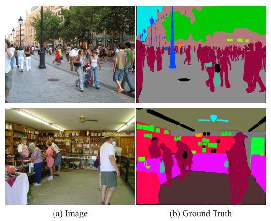
Figure 1: Illustration of complex scenes in ADE20K dataset.
图 1:ADE20K 数据集中的复杂场景示意。
Towards accurate scene perception, the knowledge graph relies on prior information of scene context. We found that the major issue for current FCN based models is lack of suitable strategy to utilize global scene category clues. For typical complex scene understanding, previously to get a global image-level feature, spatial pyramid pooling lazebnik2006beyond was widely employed where spatial statistics provide a good descriptor for overall scene interpretation. Spatial pyramid pooling network he2014spatial further enhances the ability.
要得到准确的场景感知,需要依赖场景上下文先验。我们发现,现有 FCN 类模型的主要问题是缺少合适策略利用全局场景类别线索。复杂场景理解中,为获取图像级全局特征,空间金字塔池化 lazebnik2006beyond 曾被广泛使用,空间统计可作为整体场景描述;空间金字塔池化网络 he2014spatial 又进一步增强了这一能力。
Different from these methods, to incorporate suitable global features, we propose pyramid scene parsing network (PSPNet). In addition to traditional dilated FCN chen2014semantic; yu2015multi for pixel prediction, we extend the pixel-level feature to the specially designed global pyramid pooling one. The local and global clues together make the final prediction more reliable. We also propose an optimization strategy with deeply supervised loss. We give all implementation details, which are key to our decent performance in this paper, and make the code and trained models publicly available [^1].
与上述方法不同,为融入合适的全局特征,我们提出金字塔场景解析网络(PSPNet)。在传统空洞 FCN chen2014semantic; yu2015multi 做像素预测之外,我们把像素级特征扩展为专门设计的全局金字塔池化特征。局部与全局线索共同作用,使最终预测更可靠。我们还提出带深度监督损失的优化策略,并给出实现细节——这些细节对本工作的表现至关重要——代码与训练模型亦公开[^1]。
Our approach achieves state-of-the-art performance on all available datasets. It is the champion of ImageNet scene parsing challenge 2016 zhou2016semantic, and arrived the 1st place on PASCAL VOC 2012 semantic segmentation benchmark everingham2010pascal, and the 1st place on urban scene Cityscapes data cordts2016cityscapes. They manifest that PSPNet gives a promising direction for pixel-level prediction tasks, which may even benefit CNN-based stereo matching, optical flow, depth estimation, etc. in follow-up work. Our main contributions are threefold.
本方法在各可用数据集上均达到当时最优:夺得 2016 ImageNet 场景解析挑战赛冠军 zhou2016semantic,并在 PASCAL VOC 2012 语义分割基准 everingham2010pascal 与城市场景 Cityscapes cordts2016cityscapes 上均获第一。这表明 PSPNet 为像素级预测指出了一条可行方向,后续甚至可能惠及基于 CNN 的立体匹配、光流、深度估计等。主要贡献有三。
- • We propose a pyramid scene parsing network to embed difficult scenery context features in an FCN based pixel prediction framework.
- • 提出金字塔场景解析网络,把困难场景的上下文特征嵌入基于 FCN 的像素预测框架。
- • We develop an effective optimization strategy for deep ResNet he2015deep based on deeply supervised loss.
- • 针对深度 ResNet he2015deep,设计基于深度监督损失的有效优化策略。
- • We build a practical system for state-of-the-art scene parsing and semantic segmentation where all crucial implementation details are included.
- • 构建可用于前沿场景解析与语义分割的实用系统,并纳入全部关键实现细节。
2 Related Work
2 相关工作
In the following, we review recent advances in scene parsing and semantic segmentation tasks. Driven by powerful deep neural networks krizhevsky2012imagenet; simonyan2014very; szegedy2015going; he2015deep, pixel-level prediction tasks like scene parsing and semantic segmentation achieve great progress inspired by replacing the fully-connected layer in classification with the convolution layer long2015fully. To enlarge the receptive field of neural networks, methods of chen2014semantic; yu2015multi used dilated convolution. Noh et al. noh2015learning proposed a coarse-to-fine structure with deconvolution network to learn the segmentation mask. Our baseline network is FCN and dilated network long2015fully; chen2014semantic.
下面回顾场景解析与语义分割的近期进展。在强大深度网络 krizhevsky2012imagenet; simonyan2014very; szegedy2015going; he2015deep 推动下,用卷积层替换分类网络中的全连接层 long2015fully,像素级预测任务取得显著进步。为扩大感受野,chen2014semantic; yu2015multi 采用空洞卷积。Noh et al. noh2015learning 提出由粗到精的反卷积结构学习分割掩码。我们的基线是 FCN 与空洞网络 long2015fully; chen2014semantic。
Other work mainly proceeds in two directions. One line long2015fully; chen2014semantic; chen2015attention; xia2016zoom; hariharan2015hypercolumns is with multi-scale feature ensembling. Since in deep networks, higher-layer feature contains more semantic meaning and less location information. Combining multi-scale features can improve the performance.
其他工作大致沿两条路线推进。其一 long2015fully; chen2014semantic; chen2015attention; xia2016zoom; hariharan2015hypercolumns 是多尺度特征集成:深层网络中高层特征语义更强、定位更弱,融合多尺度特征可提升表现。
The other direction is based on structure prediction. The pioneer work chen2014semantic used conditional random field (CRF) as post processing to refine the segmentation result. Following methods liu2015semantic; zheng2015conditional; arnab2016higher refined networks via end-to-end modeling. Both of the two directions ameliorate the localization ability of scene parsing where predicted semantic boundary fits objects. Yet there is still much room to exploit necessary information in complex scenes.
其二基于结构预测。先驱工作 chen2014semantic 用条件随机场(CRF)做后处理细化分割;后续 liu2015semantic; zheng2015conditional; arnab2016higher 则通过端到端建模 refining 网络。两条路线都改善了场景解析的定位能力,使预测语义边界更贴合物体,但复杂场景中仍有大量必要信息未被利用。
To make good use of global image-level priors for diverse scene understanding, methods of lazebnik2006beyond; lucchi2011spatial extracted global context information with traditional features not from deep neural networks. Similar improvement was made under object detection frameworks szegedy2014scalable. Liu et al. liu2015parsenet proved that global average pooling with FCN can improve semantic segmentation results. However, our experiments show that these global descriptors are not representative enough for the challenging ADE20K data. Therefore, different from global pooling in liu2015parsenet, we exploit the capability of global context information by different-region-based context aggregation via our pyramid scene parsing network.
为更好利用全局图像级先验理解多样场景,lazebnik2006beyond; lucchi2011spatial 用非深度特征提取全局上下文;目标检测框架中亦有类似改进 szegedy2014scalable。Liu et al. liu2015parsenet 证明 FCN 加全局平均池化可提升语义分割。但我们的实验表明,这类全局描述对挑战性的 ADE20K 仍不够代表性。因此,不同于 liu2015parsenet 的全局池化,我们通过金字塔场景解析网络,在不同区域上聚合上下文,挖掘全局上下文能力。
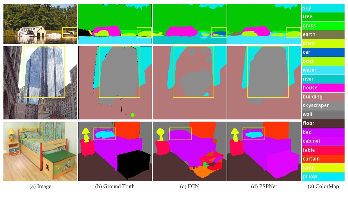
Figure 2: Scene parsing issues we observe on ADE20K zhou2016semantic dataset. The first row shows the issue of mismatched relationship – cars are seldom over water than boats. The second row shows confusion categories where class “building” is easily confused as “skyscraper”. The third row illustrates inconspicuous classes. In this example, the pillow is very similar to the bed sheet in terms of color and texture. These inconspicuous objects are easily misclassified by FCN.
图 2:我们在 ADE20K zhou2016semantic 上观察到的场景解析问题。第一行是关系错配——水面上方更常见的是船而非车。第二行是易混淆类别,「building」易与「skyscraper」混淆。第三行是不显眼类别:枕头在颜色与纹理上与床单极为接近,FCN 很容易误分。
3 Pyramid Scene Parsing Network
3 金字塔场景解析网络
We start with our observation and analysis of representative failure cases when applying FCN methods to scene parsing. They motivate proposal of our pyramid pooling module as the effective global context prior. Our pyramid scene parsing network (PSPNet) illustrated in Fig. 3 is then described to improve performance for open-vocabulary object and stuff identification in complex scene parsing.
我们先观察并分析 FCN 用于场景解析时的典型失败案例,由此引出作为有效全局上下文先验的金字塔池化模块;再描述图 3 所示的金字塔场景解析网络(PSPNet),以提升复杂场景中开放词表物体与 stuff 的识别。
3.1 Important Observations
3.1 重要观察
The new ADE20K dataset zhou2016semantic contains 150 stuff/object category labels (e.g., wall, sky, and tree) and 1,038 image-level scene descriptors (e.g., airport_terminal, bedroom, and street). So a large amount of labels and vast distributions of scenes come into existence. Inspecting the prediction results of the FCN baseline provided in zhou2016semantic, we summarize several common issues for complex-scene parsing.
新的 ADE20K zhou2016semantic 含 150 类 stuff/物体标签(如墙、天空、树)以及 1,038 个图像级场景描述(如 airport_terminal、bedroom、street),标签量大、场景分布广。审视 zhou2016semantic 提供的 FCN 基线预测,我们归纳出复杂场景解析中几类常见问题。
Mismatched Relationship
Context relationship is universal and important especially for complex scene understanding. There exist co-occurrent visual patterns. For example, an airplane is likely to be in runway or fly in sky while not over a road. For the first-row example in Fig. 2, FCN predicts the boat in the yellow box as a “car” based on its appearance. But the common knowledge is that a car is seldom over a river. Lack of the ability to collect contextual information increases the chance of misclassification.
关系错配
上下文关系在复杂场景理解中普遍且重要,存在共现视觉模式。例如飞机更可能在跑道或天空,而非悬在道路上方。图 2 第一行中,FCN 仅凭外观把黄框内的船预测为「car」,但常识是车很少出现在河面上。缺乏收集上下文的能力会提高误分概率。
Confusion Categories
There are many class label pairs in the ADE20K dataset zhou2016semantic that are confusing in classification. Examples are field and earth; mountain and hill; wall, house, building and skyscraper. They are with similar appearance. The expert annotator who labeled the entire dataset, still makes 17.60% pixel error as described in zhou2016semantic. In the second row of Fig. 2, FCN predicts the object in the box as part of skyscraper and part of building. These results should be excluded so that the whole object is either skyscraper or building, but not both. This problem can be remedied by utilizing the relationship between categories.
易混淆类别
ADE20K zhou2016semantic 中有许多易混淆的类别对,如 field 与 earth;mountain 与 hill;wall、house、building 与 skyscraper,外观相近。即便标注整个数据集的专家,按 zhou2016semantic 所述像素错误率仍达 17.60%。图 2 第二行中,FCN 把框内物体一部分标成 skyscraper、一部分标成 building;合理结果应是整块同属一类。利用类别间关系有助于缓解这一问题。
Inconspicuous Classes
Scene contains objects/stuff of arbitrary size. Several small-size things, like streetlight and signboard, are hard to find while they may be of great importance. Contrarily, big objects or stuff may exceed the receptive field of FCN and thus cause discontinuous prediction. As shown in the third row of Fig. 2, the pillow has similar appearance with the sheet. Overlooking the global scene category may fail to parse the pillow. To improve performance for remarkably small or large objects, one should pay much attention to different sub-regions that contain inconspicuous-category stuff.
不显眼类别
场景中物体/stuff 尺度任意。路灯、招牌等小物体难找却往往关键;相反,过大物体或 stuff 可能超出 FCN 感受野,造成预测不连续。图 2 第三行中枕头与床单外观相似,忽视全局场景类别就难以解析枕头。要提升显著偏小或偏大物体的表现,需要关注含不显眼类别的不同子区域。
To summarize these observations, many errors are partially or completely related to contextual relationship and global information for different receptive fields. Thus a deep network with a suitable global-scene-level prior can much improve the performance of scene parsing.
综上,许多错误都与上下文关系以及不同感受野下的全局信息有关。因此,带有合适全局场景级先验的深度网络,可显著改善场景解析。
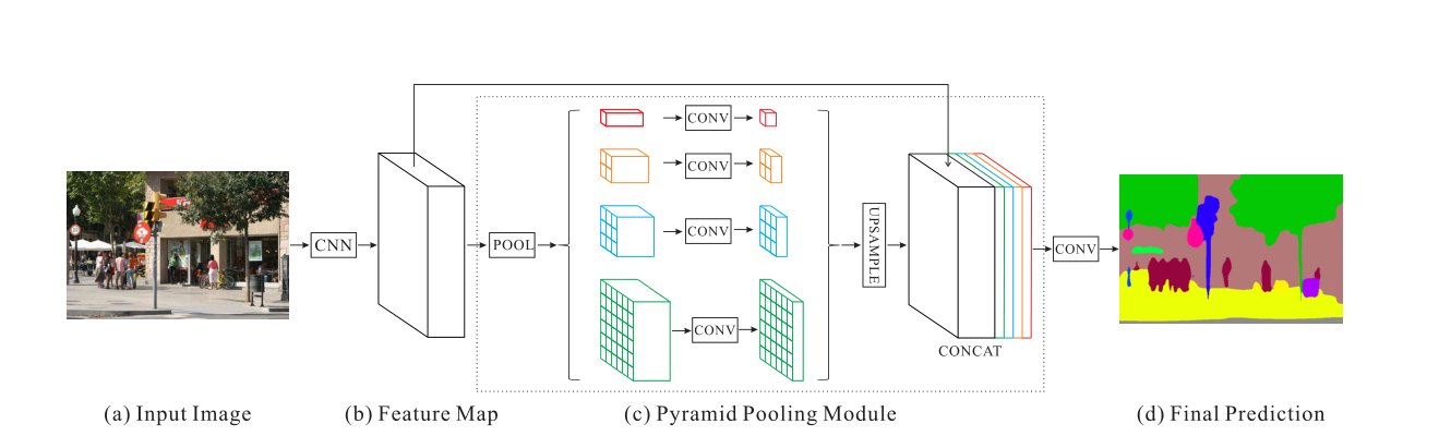
Figure 3: Overview of our proposed PSPNet. Given an input image (a), we first use CNN to get the feature map of the last convolutional layer (b), then a pyramid parsing module is applied to harvest different sub-region representations, followed by upsampling and concatenation layers to form the final feature representation, which carries both local and global context information in (c). Finally, the representation is fed into a convolution layer to get the final per-pixel prediction (d).
图 3:所提 PSPNet 总览。给定输入图像 (a),先用 CNN 得到最后一层卷积特征图 (b),再经金字塔解析模块收集不同子区域表示,上采样并拼接形成同时携带局部与全局上下文的最终特征 (c),最后送入卷积层得到逐像素预测 (d)。
3.2 Pyramid Pooling Module
3.2 金字塔池化模块
With above analysis, in what follows, we introduce the pyramid pooling module, which empirically proves to be an effective global contextual prior.
基于上述分析,下面介绍金字塔池化模块;实验表明它是有效的全局上下文先验。
In a deep neural network, the size of receptive field can roughly indicates how much we use context information. Although theoretically the receptive field of ResNet he2015deep is already larger than the input image, it is shown by Zhou et al. zhou2014object that the empirical receptive field of CNN is much smaller than the theoretical one especially on high-level layers. This makes many networks not sufficiently incorporate the momentous global scenery prior. We address this issue by proposing an effective global prior representation.
在深度网络中,感受野大小大致反映可用上下文多少。尽管 ResNet he2015deep 的理论感受野已大于输入图像,Zhou et al. zhou2014object 指出 CNN 的经验感受野远小于理论值,高层尤甚,导致许多网络未能充分纳入关键的全局场景先验。我们提出有效的全局先验表示来应对。
Global average pooling is a good baseline model as the global contextual prior, which is commonly used in image classification tasks szegedy2015going; he2015deep. In liu2015parsenet, it was successfully applied to semantic segmentation. But regarding the complex-scene images in ADE20K zhou2016semantic, this strategy is not enough to cover necessary information. Pixels in these scene images are annotated regarding many stuff and objects. Directly fusing them to form a single vector may lose the spatial relation and cause ambiguity. Global context information along with sub-region context is helpful in this regard to distinguish among various categories. A more powerful representation could be fused information from different sub-regions with these receptive fields. Similar conclusion was drawn in classical work lazebnik2006beyond; he2014spatial of scene/image classification.
全局平均池化是常见的全局上下文先验基线,广泛用于图像分类 szegedy2015going; he2015deep,并在 liu2015parsenet 中成功用于语义分割。但对 ADE20K zhou2016semantic 这类复杂场景,仅此不够:像素按众多 stuff 与物体标注,直接融成单一向量会丢失空间关系并造成歧义。此时需要全局上下文与子区域上下文共同帮助区分类别。融合不同感受野下各子区域的信息,可得到更强表示;经典场景/图像分类工作 lazebnik2006beyond; he2014spatial 亦有类似结论。
In he2014spatial, feature maps in different levels generated by pyramid pooling were finally flattened and concatenated to be fed into a fully connected layer for classification. This global prior is designed to remove the fixed-size constraint of CNN for image classification. To further reduce context information loss between different sub-regions, we propose a hierarchical global prior, containing information with different scales and varying among different sub-regions. We call it pyramid pooling module for global scene prior construction upon the final-layer-feature-map of the deep neural network, as illustrated in part (c) of Fig. 3.
在 he2014spatial 中,金字塔池化得到的多层特征图最终展平拼接后送入全连接层做分类,该全局先验用于解除 CNN 分类的固定尺寸约束。为进一步减少不同子区域间的上下文损失,我们提出层次化全局先验,包含不同尺度、并随子区域变化的信息,称为金字塔池化模块,在深度网络最终层特征图上构建全局场景先验,见图 3(c)。
The pyramid pooling module fuses features under four different pyramid scales. The coarsest level highlighted in red is global pooling to generate a single bin output. The following pyramid level separates the feature map into different sub-regions and forms pooled representation for different locations. The output of different levels in the pyramid pooling module contains the feature map with varied sizes. To maintain the weight of global feature, we use convolution layer after each pyramid level to reduce the dimension of context representation to of the original one if the level size of pyramid is . Then we directly upsample the low-dimension feature maps to get the same size feature as the original feature map via bilinear interpolation. Finally, different levels of features are concatenated as the final pyramid pooling global feature.
金字塔池化模块在四个金字塔尺度上融合特征。最粗一层(红色)做全局池化,输出单一 bin;随后各层把特征图划分为不同子区域,形成各位置的池化表示。各级输出特征图尺寸不同。为保持全局特征权重,若金字塔层级数为 ,我们在每一级后接 卷积,把上下文表示维数压到原来的 。再用双线性插值把低维特征图上采样到与原始特征图同尺寸,最后拼接各级特征,得到最终的金字塔池化全局特征。
Noted that the number of pyramid levels and size of each level can be modified. They are related to the size of feature map that is fed into the pyramid pooling layer. The structure abstracts different sub-regions by adopting varying-size pooling kernels in a few strides. Thus the multi-stage kernels should maintain a reasonable gap in representation. Our pyramid pooling module is a four-level one with bin sizes of , , and respectively. For the type of pooling operation between max and average, we perform extensive experiments to show the difference in Section 5.2.
需要说明,金字塔层级数与每级尺寸可改,取决于送入金字塔池化层的特征图大小。该结构通过若干步长下不同尺寸的池化核抽象不同子区域,多级核之间应保持合理表征间距。我们的金字塔池化模块为四级,bin 尺寸分别为 、、 与 。池化在 max 与 average 之间的选择,详见第 5.2 节实验。
3.3 Network Architecture
3.3 网络结构
With the pyramid pooling module, we propose our pyramid scene parsing network (PSPNet) as illustrated in Fig. 3. Given an input image in Fig. 3(a), we use a pretrained ResNet he2015deep model with the dilated network strategy chen2014semantic; yu2015multi to extract the feature map. The final feature map size is of the input image, as shown in Fig. 3(b). On top of the map, we use the pyramid pooling module shown in (c) to gather context information. Using our 4-level pyramid, the pooling kernels cover the whole, half of, and small portions of the image. They are fused as the global prior. Then we concatenate the prior with the original feature map in the final part of (c). It is followed by a convolution layer to generate the final prediction map in (d).
结合金字塔池化模块,我们提出图 3 所示的金字塔场景解析网络(PSPNet)。对图 3(a) 输入,用带空洞策略 chen2014semantic; yu2015multi 的预训练 ResNet he2015deep 提取特征,最终特征图为输入的 ,见图 3(b)。其上施加 (c) 中的金字塔池化模块收集上下文:四级池化核分别覆盖整图、半图与更小局部,融合为全局先验,再与原始特征图在 (c) 末尾拼接,经卷积得到 (d) 中的最终预测图。
To explain our structure, PSPNet provides an effective global contextual prior for pixel-level scene parsing. The pyramid pooling module can collect levels of information, more representative than global pooling liu2015parsenet. In terms of computational cost, our PSPNet does not much increase it compared to the original dilated FCN network. In end-to-end learning, the global pyramid pooling module and the local FCN feature can be optimized simultaneously.
结构上,PSPNet 为像素级场景解析提供有效全局上下文先验;金字塔池化模块可收集多级信息,比全局池化 liu2015parsenet 更具代表性。计算开销相对原始空洞 FCN 增加不多。端到端学习中,全局金字塔池化与局部 FCN 特征可同时优化。
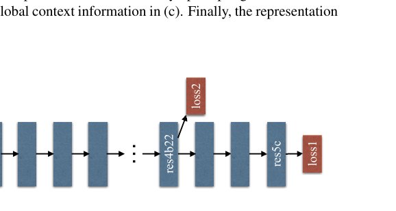
Figure 4: Illustration of auxiliary loss in ResNet101. Each blue box denotes a residue block. The auxiliary loss is added after the res4b22 residue block.
图 4:ResNet101 中辅助损失示意。每个蓝框表示一个残差块;辅助损失加在 res4b22 残差块之后。
4 Deep Supervision for ResNet-Based FCN
4 面向基于 ResNet 的 FCN 的深度监督
Deep pretrained networks lead to good performance krizhevsky2012imagenet; simonyan2014very; he2015deep. However, increasing depth of the network may introduce additional optimization difficulty as shown in shen2016relay; lee2015deeply for image classification. ResNet solves this problem with skip connection in each block. Latter layers of deep ResNet mainly learn residues based on previous ones.
深度预训练网络带来良好表现 krizhevsky2012imagenet; simonyan2014very; he2015deep。但如 shen2016relay; lee2015deeply 在图像分类中所示,加深网络可能引入额外优化困难。ResNet 用各块内的跳跃连接缓解这一问题,深层主要在前层基础上学习残差。
We contrarily propose generating initial results by supervision with an additional loss, and learning the residue afterwards with the final loss. Thus, optimization of the deep network is decomposed into two, each is simpler to solve.
我们则提出:先用额外损失监督生成初始结果,再用最终损失学习其后残差,从而把深度网络优化拆成两个更易求解的问题。
An example of our deeply supervised ResNet101 he2015deep model is illustrated in Fig. 4. Apart from the main branch using softmax loss to train the final classifier, another classifier is applied after the fourth stage, i.e., the res4b22 residue block. Different from relay backpropagation shen2016relay that blocks the backward auxiliary loss to several shallow layers, we let the two loss functions pass through all previous layers. The auxiliary loss helps optimize the learning process, while the master branch loss takes the most responsibility. We add weight to balance the auxiliary loss.
图 4 给出深度监督 ResNet101 he2015deep 的例子。除主分支用 softmax 损失训练最终分类器外,在第四阶段(即 res4b22 残差块)后再接一个分类器。与阻断辅助损失回传到若干浅层的 relay backpropagation shen2016relay 不同,我们让两个损失都穿过此前全部层。辅助损失帮助优化学习过程,主分支损失仍承担主要责任;并对辅助损失加权以平衡。
In the testing phase, we abandon this auxiliary branch and only use the well optimized master branch for final prediction. This kind of deeply supervised training strategy for ResNet-based FCN is broadly useful under different experimental settings and works with the pre-trained ResNet model. This manifests the generality of such a learning strategy. More details are provided in Section 5.2.
测试时去掉辅助分支,只用优化好的主分支做最终预测。这种面向基于 ResNet 的 FCN 的深度监督训练策略,在多种实验设定下普遍有用,并与预训练 ResNet 兼容,说明其通用性。更多细节见第 5.2 节。
5 Experiments
5 实验
Our proposed method is successful on scene parsing and semantic segmentation challenges. We evaluate it in this section on three different datasets, including ImageNet scene parsing challenge 2016 zhou2016semantic, PASCAL VOC 2012 semantic segmentation everingham2010pascal and urban scene understanding dataset Cityscapes cordts2016cityscapes.
所提方法在场景解析与语义分割挑战中表现突出。本节在三个数据集上评测:2016 ImageNet 场景解析挑战 zhou2016semantic、PASCAL VOC 2012 语义分割 everingham2010pascal,以及城市场景 Cityscapes cordts2016cityscapes。
5.1 Implementation Details
5.1 实现细节
For a practical deep learning system, devil is always in the details. Our implementation is based on the public platform Caffe jia2014caffe. Inspired by chen2016deeplab, we use the “poly” learning rate policy where current learning rate equals to the base one multiplying . We set base learning rate to 0.01 and power to 0.9. The performance can be improved by increasing the iteration number, which is set to 150K for ImageNet experiment, 30K for PASCAL VOC and 90K for Cityscapes. Momentum and weight decay are set to 0.9 and 0.0001 respectively. For data augmentation, we adopt random mirror and random resize between 0.5 and 2 for all datasets, and additionally add random rotation between -10 and 10 degrees, and random Gaussian blur for ImageNet and PASCAL VOC. This comprehensive data augmentation scheme makes the network resist overfitting. Our network contains dilated convolution following chen2016deeplab.
实用深度学习系统总是细节决定成败。实现基于公开平台 Caffe jia2014caffe。受 chen2016deeplab 启发,采用 “poly” 学习率策略:当前学习率 = 基础学习率 。基础学习率设为 0.01,power 为 0.9。增加迭代通常可提升表现:ImageNet 实验 150K,PASCAL VOC 30K,Cityscapes 90K。动量与权重衰减分别为 0.9 与 0.0001。数据增强上,全部数据集使用随机镜像与 0.5–2 的随机缩放;ImageNet 与 PASCAL VOC 另加 -10° 到 10° 随机旋转与随机高斯模糊。这套增强有助于抑制过拟合。网络还按 chen2016deeplab 使用空洞卷积。
During the course of experiments, we notice that an appropriately large “cropsize” can yield good performance and “batchsize” in the batch normalization ioffe2015batch layer is of great importance. Due to limited physical memory on GPU cards, we set the “batchsize” to 16 during training. To achieve this, we modify Caffe from wang2015towards together with branch chen2016deeplab and make it support batch normalization on data gathered from multiple GPUs based on OpenMPI. For the auxiliary loss, we set the weight to 0.4 in experiments.
实验中我们发现,适当偏大的 cropsize 有利于表现,且批归一化 ioffe2015batch 层中的 batchsize 十分关键。受 GPU 显存限制,训练 batchsize 设为 16。为此我们修改来自 wang2015towards 以及分支 chen2016deeplab 的 Caffe,基于 OpenMPI 支持跨多卡汇聚数据的批归一化。辅助损失权重实验中设为 0.4。
5.2 ImageNet Scene Parsing Challenge 2016
5.2 2016 ImageNet 场景解析挑战
Dataset and Evaluation Metrics
The ADE20K dataset zhou2016semantic is used in ImageNet scene parsing challenge 2016. Different from other datasets, ADE20K is more challenging for the up to 150 classes and diverse scenes with a total of 1,038 image-level labels. The challenge data is divided into 20K/2K/3K images for training, validation and testing. Also, it needs to parse both objects and stuff in the scene, which makes it more difficult than other datasets. For evaluation, both pixel-wise accuracy (Pixel Acc.) and mean of class-wise intersection over union (Mean IoU) are used.
数据集与评价指标
2016 ImageNet 场景解析挑战使用 ADE20K zhou2016semantic。与其他数据集不同,ADE20K 多达 150 类、场景多样,并有共 1,038 个图像级标签,挑战更大。数据划分为训练/验证/测试 20K/2K/3K 张,且需同时解析场景中的物体与 stuff。评价采用像素精度(Pixel Acc.)与类别平均交并比(Mean IoU)。
| Method | Mean IoU(%) | Pixel Acc.(%) |
|---|---|---|
| ResNet50-Baseline | 37.23 | 78.01 |
| ResNet50+B1+MAX | 39.94 | 79.46 |
| ResNet50+B1+AVE | 40.07 | 79.52 |
| ResNet50+B1236+MAX | 40.18 | 79.45 |
| ResNet50+B1236+AVE | 41.07 | 79.97 |
| ResNet50+B1236+MAX+DR | 40.87 | 79.61 |
| ResNet50+B1236+AVE+DR | 41.68 | 80.04 |
Table 1: Investigation of PSPNet with different settings. Baseline is ResNet50-based FCN with dilated network. ‘B1’ and ‘B1236’ denote pooled feature maps of bin sizes and respectively. ‘MAX’ and ‘AVE’ represent max pooling and average pooling operations individually. ‘DR’ means that dimension reduction is taken after pooling. The results are tested on the validation set with the single-scale input.
| 方法 | Mean IoU(%) | Pixel Acc.(%) |
|---|---|---|
| ResNet50-Baseline | 37.23 | 78.01 |
| ResNet50+B1+MAX | 39.94 | 79.46 |
| ResNet50+B1+AVE | 40.07 | 79.52 |
| ResNet50+B1236+MAX | 40.18 | 79.45 |
| ResNet50+B1236+AVE | 41.07 | 79.97 |
| ResNet50+B1236+MAX+DR | 40.87 | 79.61 |
| ResNet50+B1236+AVE+DR | 41.68 | 80.04 |
表 1:不同设定下 PSPNet 的考察。基线为带空洞的 ResNet50 FCN。‘B1’ 与 ‘B1236’ 分别表示 bin 尺寸为 与 的池化特征。‘MAX’/‘AVE’ 为最大/平均池化。‘DR’ 表示池化后做了维数削减。结果在验证集上、单尺度输入测得。
Ablation Study for PSPNet
To evaluate PSPNet, we conduct experiments with several settings, including pooling types of max and average, pooling with just one global feature or four-level features, with and without dimension reduction after the pooling operation and before concatenation. As listed in Table 1, average pooling works better than max pooling in all settings. Pooling with pyramid parsing outperforms that using global pooling. With dimension reduction, the performance is further enhanced. With our proposed PSPNet, the best setting yields results 41.68/80.04 in terms of Mean IoU and Pixel Acc. (%), exceeding global average pooling of 40.07/79.52 as idea in Liu et al. liu2015parsenet by 1.61/0.52. And compared to the baseline, PSPNet outperforming it by 4.45/2.03 in terms of absolute improvement and 11.95/2.60 in terms of relative difference.
PSPNet 消融
为评估 PSPNet,我们试验多种设定:max 与 average 池化、仅用单一全局特征或四级特征、池化后拼接前是否维数削减。如表 1,各设定下平均池化均优于最大池化;金字塔解析池化优于仅全局池化;加维数削减后表现再升。最佳设定 Mean IoU / Pixel Acc.(%)为 41.68/80.04,相对 Liu et al. liu2015parsenet 思路下的全局平均池化 40.07/79.52 高出 1.61/0.52;相对基线绝对提升 4.45/2.03,相对提升 11.95%/2.60%。
| Loss Weight | Mean IoU(%) | Pixel Acc.(%) |
|---|---|---|
| ResNet50 (without AL) | 35.82 | 77.07 |
| ResNet50 (with = 0.3) | 37.01 | 77.87 |
| ResNet50 (with = 0.4) | 37.23 | 78.01 |
| ResNet50 (with = 0.6) | 37.09 | 77.84 |
| ResNet50 (with = 0.9) | 36.99 | 77.87 |
Table 2: Setting an appropriate loss weight in the auxiliary branch is important. ‘AL’ denotes the auxiliary loss. Baseline is ResNet50-based FCN with dilated network. Empirically, = 0.4 yields the best performance. The results are tested on the validation set with the single-scale input.
| 损失权重 | Mean IoU(%) | Pixel Acc.(%) |
|---|---|---|
| ResNet50(无 AL) | 35.82 | 77.07 |
| ResNet50( = 0.3) | 37.01 | 77.87 |
| ResNet50( = 0.4) | 37.23 | 78.01 |
| ResNet50( = 0.6) | 37.09 | 77.84 |
| ResNet50( = 0.9) | 36.99 | 77.87 |
表 2:辅助分支损失权重 需设得恰当。‘AL’ 表示辅助损失。基线为带空洞的 ResNet50 FCN。经验上 = 0.4 最好。结果在验证集上、单尺度输入测得。
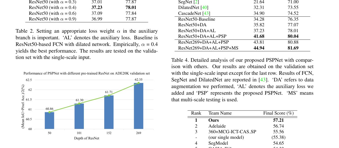
Figure 5: Performance grows with deeper networks. The results are obtained on the validation set with the single-scale input.
图 5:网络加深时表现提升。结果在验证集上、单尺度输入测得。
| Method | Mean IoU(%) | Pixel Acc.(%) |
|---|---|---|
| PSPNet(50) | 41.68 | 80.04 |
| PSPNet(101) | 41.96 | 80.64 |
| PSPNet(152) | 42.62 | 80.80 |
| PSPNet(269) | 43.81 | 80.88 |
| PSPNet(50)+MS | 42.78 | 80.76 |
| PSPNet(101)+MS | 43.29 | 81.39 |
| PSPNet(152)+MS | 43.51 | 81.38 |
| PSPNet(269)+MS | 44.94 | 81.69 |
Table 3: Deeper pre-trained model get higher performance. Number in the brackets refers to the depth of ResNet and ‘MS’ denotes multi-scale testing.
| 方法 | Mean IoU(%) | Pixel Acc.(%) |
|---|---|---|
| PSPNet(50) | 41.68 | 80.04 |
| PSPNet(101) | 41.96 | 80.64 |
| PSPNet(152) | 42.62 | 80.80 |
| PSPNet(269) | 43.81 | 80.88 |
| PSPNet(50)+MS | 42.78 | 80.76 |
| PSPNet(101)+MS | 43.29 | 81.39 |
| PSPNet(152)+MS | 43.51 | 81.38 |
| PSPNet(269)+MS | 44.94 | 81.69 |
表 3:更深预训练模型带来更高表现。括号内为 ResNet 深度,‘MS’ 表示多尺度测试。
| Method | Mean IoU(%) | Pixel Acc.(%) |
|---|---|---|
| FCN long2015fully | 29.39 | 71.32 |
| SegNet badrinarayanan2015segnet | 21.64 | 71.00 |
| DilatedNet yu2015multi | 32.31 | 73.55 |
| CascadeNet zhou2016semantic | 34.90 | 74.52 |
| ResNet50-Baseline | 34.28 | 76.35 |
| ResNet50+DA | 35.82 | 77.07 |
| ResNet50+DA+AL | 37.23 | 78.01 |
| ResNet50+DA+AL+PSP | 41.68 | 80.04 |
| ResNet269+DA+AL+PSP | 43.81 | 80.88 |
| ResNet269+DA+AL+PSP+MS | 44.94 | 81.69 |
Table 4: Detailed analysis of our proposed PSPNet with comparison with others. Our results are obtained on the validation set with the single-scale input except for the last row. Results of FCN, SegNet and DilatedNet are reported in zhou2016semantic. ‘DA’ refers to data augmentation we performed, ‘AL’ denotes the auxiliary loss we added and ‘PSP’ represents the proposed PSPNet. ‘MS’ means that multi-scale testing is used.
| 方法 | Mean IoU(%) | Pixel Acc.(%) |
|---|---|---|
| FCN long2015fully | 29.39 | 71.32 |
| SegNet badrinarayanan2015segnet | 21.64 | 71.00 |
| DilatedNet yu2015multi | 32.31 | 73.55 |
| CascadeNet zhou2016semantic | 34.90 | 74.52 |
| ResNet50-Baseline | 34.28 | 76.35 |
| ResNet50+DA | 35.82 | 77.07 |
| ResNet50+DA+AL | 37.23 | 78.01 |
| ResNet50+DA+AL+PSP | 41.68 | 80.04 |
| ResNet269+DA+AL+PSP | 43.81 | 80.88 |
| ResNet269+DA+AL+PSP+MS | 44.94 | 81.69 |
表 4:所提 PSPNet 的细化分析及与其他方法对比。除末行外均为验证集单尺度结果。FCN、SegNet、DilatedNet 结果引自 zhou2016semantic。‘DA’ 为数据增强,‘AL’ 为辅助损失,‘PSP’ 为所提 PSPNet,‘MS’ 为多尺度测试。
| Rank | Team Name | Final Score (%) |
|---|---|---|
| 1 | Ours | 57.21 |
| 2 | Adelaide | 56.74 |
| 3 | 360+MCG-ICT-CAS_SP | 55.56 |
| - | (our single model) | (55.38) |
| 4 | SegModel | 54.65 |
| 5 | CASIA_IVA | 54.33 |
| - | DilatedNet yu2015multi | 45.67 |
| - | FCN long2015fully | 44.80 |
| - | SegNet badrinarayanan2015segnet | 40.79 |
Table 5: Results of ImageNet scene parsing challenge 2016. The best entry of each team is listed. The final score is the mean of Mean IoU and Pixel Acc. Results are evaluated on the testing set.
| 名次 | 队伍 | 最终得分 (%) |
|---|---|---|
| 1 | Ours | 57.21 |
| 2 | Adelaide | 56.74 |
| 3 | 360+MCG-ICT-CAS_SP | 55.56 |
| - | (我们的单模型) | (55.38) |
| 4 | SegModel | 54.65 |
| 5 | CASIA_IVA | 54.33 |
| - | DilatedNet yu2015multi | 45.67 |
| - | FCN long2015fully | 44.80 |
| - | SegNet badrinarayanan2015segnet | 40.79 |
表 5:2016 ImageNet 场景解析挑战结果。列出各队最佳提交。最终得分为 Mean IoU 与 Pixel Acc. 的均值。在测试集上评测。
Ablation Study for Auxiliary Loss
The introduced auxiliary loss helps optimize the learning process while not influencing learning in the master branch. We experiment with setting the auxiliary loss weight between 0 and 1 and show the results in Table 2. The baseline uses ResNet50-based FCN with dilated network, with the master branch’s softmax loss for optimization. Adding the auxiliary loss branch, = 0.4 yields the best performance. It outperforms the baseline with an improvement of 1.41/0.94 in terms of Mean IoU and Pixel Acc. (%). We believe deeper networks will benefit more given the new augmented auxiliary loss.
辅助损失消融
引入的辅助损失帮助优化学习过程,同时不干扰主分支学习。我们将辅助损失权重 在 0 到 1 间取值,结果见表 2。基线为带空洞的 ResNet50 FCN,仅用主分支 softmax 优化。加入辅助分支后, = 0.4 最好,相对基线 Mean IoU / Pixel Acc.(%)提升 1.41/0.94。我们相信更深网络在该增强辅助损失下收益更大。
Ablation Study for Pre-trained Model
Deeper neural networks have been shown in previous work to be beneficial to large scale data classification. To further analyze PSPNet, we conduct experiments for different depths of pre-trained ResNet. We test four depths of {50, 101, 152, 269}. As shown in Fig. 5, with the same setting, increasing the depth of ResNet from 50 to 269 can improve the score of (Mean IoU + Pixel Acc.) / 2 (%) from 60.86 to 62.35, with 1.49 absolute improvement. Detailed scores of PSPNet pre-trained from different depth ResNet models are listed in Table 3.
预训练模型消融
既往工作表明更深网络有利于大规模分类。为进一步分析 PSPNet,我们在预训练 ResNet 深度 上实验。如图 5,相同设定下深度从 50 增至 269,(Mean IoU + Pixel Acc.)/2(%)从 60.86 升至 62.35,绝对提升 1.49。不同深度预训练下 PSPNet 的详细分数见表 3。
More Detailed Performance Analysis
We show our more detailed analysis on the validation set of ADE20K in Table 4. All our results except the last-row one use single-scale test. “ResNet269+DA+AL+PSP+MS” uses multi-scale testing. Our baseline is adapted from ResNet50 with dilated network, which yields MeanIoU 34.28 and Pixel Acc. 76.35. It already outperforms other prior systems possibly due to the powerful ResNet he2015deep.
更细的表现分析
表 4 给出 ADE20K 验证集上更细的分析。除末行外均为单尺度测试;“ResNet269+DA+AL+PSP+MS” 使用多尺度测试。基线由 ResNet50 加空洞得到,MeanIoU 34.28、Pixel Acc. 76.35,已可能因 ResNet he2015deep 的能力而超过若干先前系统。
Our proposed architecture makes further improvement compared to the baseline. Using data augmentation, our result exceeds the baseline by 1.54/0.72 and reaches 35.82/77.07. Using the auxiliary loss can further improve it by 1.41/0.94 and reaches 37.23/78.01. With PSPNet, we notice relatively more significant progress for improvement of 4.45/2.03. The result reaches 41.68/80.04. The difference from the baseline result is 7.40/3.69 in terms of absolute improvement and 21.59/4.83 (%) in terms of relativity. A deeper network of ResNet269 yields even higher performance up to 43.81/80.88. Finally, the multi-scale testing scheme moves the scores to 44.94/81.69.
相对基线,所提结构继续提升。数据增强后超过基线 1.54/0.72,达到 35.82/77.07;再加辅助损失提升 1.41/0.94,达到 37.23/78.01;加上 PSPNet 提升更明显,为 4.45/2.03,达到 41.68/80.04。相对基线绝对差 7.40/3.69,相对提升 21.59%/4.83%。更深的 ResNet269 可达 43.81/80.88;多尺度测试最终到 44.94/81.69。
Results in Challenge
Using the proposed architecture, our team came in the 1st place in ImageNet scene parsing challenge 2016. Table 5 shows a few results in this competition. Our ensemble submission achieves score 57.21% on the testing set. Our single-model yields score 55.38%, which is even higher than a few other multi-model ensemble submissions. This score is lower than that on the validation set possibly due to the difference of data distributions between validation and testing sets. As shown in column (d) of Fig. 2, PSPNet solves the common problems in FCN. Fig. 6 shows another few parsing results on validation set of ADE20K. Our results contain more accurate and detailed structures compared to the baseline.
挑战赛结果
借助所提结构,我们队在 2016 ImageNet 场景解析挑战中获第一。表 5 列出部分结果:集成提交测试集得分 57.21%;单模型 55.38%,甚至高于若干多模型集成。该分数低于验证集,可能因验证与测试分布差异。如图 2(d) 列所示,PSPNet 缓解了 FCN 的常见问题。图 6 另给出 ADE20K 验证集若干解析结果,相对基线结构更准、更细。
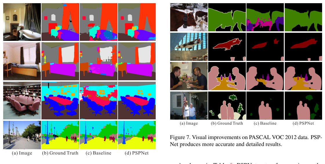
Figure 6: Visual improvements on ADE20K, PSPNet produces more accurate and detailed results.
图 6:ADE20K 上的视觉改进,PSPNet 结果更准确、细节更丰富。
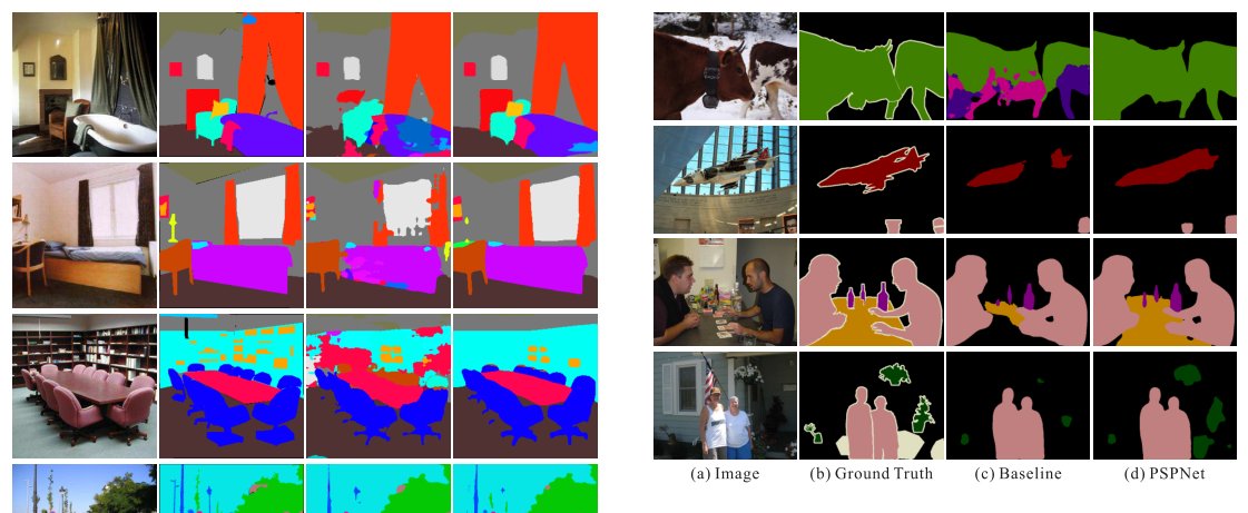
Figure 7: Visual improvements on PASCAL VOC 2012 data. PSPNet produces more accurate and detailed results.
图 7:PASCAL VOC 2012 上的视觉改进,PSPNet 结果更准确、细节更丰富。
| Method | aero | bike | bird | boat | bottle | bus | car | cat | chair | cow | table | dog | horse | mbike | person | plant | sheep | sofa | train | tv | mIoU |
|---|---|---|---|---|---|---|---|---|---|---|---|---|---|---|---|---|---|---|---|---|---|
| FCN long2015fully | 76.8 | 34.2 | 68.9 | 49.4 | 60.3 | 75.3 | 74.7 | 77.6 | 21.4 | 62.5 | 46.8 | 71.8 | 63.9 | 76.5 | 73.9 | 45.2 | 72.4 | 37.4 | 70.9 | 55.1 | 62.2 |
| Zoom-out mostajabi2015feedforward | 85.6 | 37.3 | 83.2 | 62.5 | 66.0 | 85.1 | 80.7 | 84.9 | 27.2 | 73.2 | 57.5 | 78.1 | 79.2 | 81.1 | 77.1 | 53.6 | 74.0 | 49.2 | 71.7 | 63.3 | 69.6 |
| DeepLab chen2014semantic | 84.4 | 54.5 | 81.5 | 63.6 | 65.9 | 85.1 | 79.1 | 83.4 | 30.7 | 74.1 | 59.8 | 79.0 | 76.1 | 83.2 | 80.8 | 59.7 | 82.2 | 50.4 | 73.1 | 63.7 | 71.6 |
| CRF-RNN zheng2015conditional | 87.5 | 39.0 | 79.7 | 64.2 | 68.3 | 87.6 | 80.8 | 84.4 | 30.4 | 78.2 | 60.4 | 80.5 | 77.8 | 83.1 | 80.6 | 59.5 | 82.8 | 47.8 | 78.3 | 67.1 | 72.0 |
| DeconvNet noh2015learning | 89.9 | 39.3 | 79.7 | 63.9 | 68.2 | 87.4 | 81.2 | 86.1 | 28.5 | 77.0 | 62.0 | 79.0 | 80.3 | 83.6 | 80.2 | 58.8 | 83.4 | 54.3 | 80.7 | 65.0 | 72.5 |
| GCRF vemulapalli2016gaussian | 85.2 | 43.9 | 83.3 | 65.2 | 68.3 | 89.0 | 82.7 | 85.3 | 31.1 | 79.5 | 63.3 | 80.5 | 79.3 | 85.5 | 81.0 | 60.5 | 85.5 | 52.0 | 77.3 | 65.1 | 73.2 |
| DPN liu2015semantic | 87.7 | 59.4 | 78.4 | 64.9 | 70.3 | 89.3 | 83.5 | 86.1 | 31.7 | 79.9 | 62.6 | 81.9 | 80.0 | 83.5 | 82.3 | 60.5 | 83.2 | 53.4 | 77.9 | 65.0 | 74.1 |
| Piecewise lin2015efficient | 90.6 | 37.6 | 80.0 | 67.8 | 74.4 | 92.0 | 85.2 | 86.2 | 39.1 | 81.2 | 58.9 | 83.8 | 83.9 | 84.3 | 84.8 | 62.1 | 83.2 | 58.2 | 80.8 | 72.3 | 75.3 |
| PSPNet | 91.8 | 71.9 | 94.7 | 71.2 | 75.8 | 95.2 | 89.9 | 95.9 | 39.3 | 90.7 | 71.7 | 90.5 | 94.5 | 88.8 | 89.6 | 72.8 | 89.6 | 64.0 | 85.1 | 76.3 | 82.6 |
| CRF-RNN*†* zheng2015conditional | 90.4 | 55.3 | 88.7 | 68.4 | 69.8 | 88.3 | 82.4 | 85.1 | 32.6 | 78.5 | 64.4 | 79.6 | 81.9 | 86.4 | 81.8 | 58.6 | 82.4 | 53.5 | 77.4 | 70.1 | 74.7 |
| BoxSup*†* dai2015boxsup | 89.8 | 38.0 | 89.2 | 68.9 | 68.0 | 89.6 | 83.0 | 87.7 | 34.4 | 83.6 | 67.1 | 81.5 | 83.7 | 85.2 | 83.5 | 58.6 | 84.9 | 55.8 | 81.2 | 70.7 | 75.2 |
| Dilation8*†* yu2015multi | 91.7 | 39.6 | 87.8 | 63.1 | 71.8 | 89.7 | 82.9 | 89.8 | 37.2 | 84.0 | 63.0 | 83.3 | 89.0 | 83.8 | 85.1 | 56.8 | 87.6 | 56.0 | 80.2 | 64.7 | 75.3 |
| DPN*†* liu2015semantic | 89.0 | 61.6 | 87.7 | 66.8 | 74.7 | 91.2 | 84.3 | 87.6 | 36.5 | 86.3 | 66.1 | 84.4 | 87.8 | 85.6 | 85.4 | 63.6 | 87.3 | 61.3 | 79.4 | 66.4 | 77.5 |
| Piecewise*†* lin2015efficient | 94.1 | 40.7 | 84.1 | 67.8 | 75.9 | 93.4 | 84.3 | 88.4 | 42.5 | 86.4 | 64.7 | 85.4 | 89.0 | 85.8 | 86.0 | 67.5 | 90.2 | 63.8 | 80.9 | 73.0 | 78.0 |
| FCRNs*†* wu2016bridging | 91.9 | 48.1 | 93.4 | 69.3 | 75.5 | 94.2 | 87.5 | 92.8 | 36.7 | 86.9 | 65.2 | 89.1 | 90.2 | 86.5 | 87.2 | 64.6 | 90.1 | 59.7 | 85.5 | 72.7 | 79.1 |
| LRR*†* ghiasi2016laplacian | 92.4 | 45.1 | 94.6 | 65.2 | 75.8 | 95.1 | 89.1 | 92.3 | 39.0 | 85.7 | 70.4 | 88.6 | 89.4 | 88.6 | 86.6 | 65.8 | 86.2 | 57.4 | 85.7 | 77.3 | 79.3 |
| DeepLab*†* chen2016deeplab | 92.6 | 60.4 | 91.6 | 63.4 | 76.3 | 95.0 | 88.4 | 92.6 | 32.7 | 88.5 | 67.6 | 89.6 | 92.1 | 87.0 | 87.4 | 63.3 | 88.3 | 60.0 | 86.8 | 74.5 | 79.7 |
| PSPNet*†* | 95.8 | 72.7 | 95.0 | 78.9 | 84.4 | 94.7 | 92.0 | 95.7 | 43.1 | 91.0 | 80.3 | 91.3 | 96.3 | 92.3 | 90.1 | 71.5 | 94.4 | 66.9 | 88.8 | 82.0 | 85.4 |
Table 6: Per-class results on PASCAL VOC 2012 testing set. Methods pre-trained on MS-COCO are marked with ‘†’.
| 方法 | aero | bike | bird | boat | bottle | bus | car | cat | chair | cow | table | dog | horse | mbike | person | plant | sheep | sofa | train | tv | mIoU |
|---|---|---|---|---|---|---|---|---|---|---|---|---|---|---|---|---|---|---|---|---|---|
| FCN long2015fully | 76.8 | 34.2 | 68.9 | 49.4 | 60.3 | 75.3 | 74.7 | 77.6 | 21.4 | 62.5 | 46.8 | 71.8 | 63.9 | 76.5 | 73.9 | 45.2 | 72.4 | 37.4 | 70.9 | 55.1 | 62.2 |
| Zoom-out mostajabi2015feedforward | 85.6 | 37.3 | 83.2 | 62.5 | 66.0 | 85.1 | 80.7 | 84.9 | 27.2 | 73.2 | 57.5 | 78.1 | 79.2 | 81.1 | 77.1 | 53.6 | 74.0 | 49.2 | 71.7 | 63.3 | 69.6 |
| DeepLab chen2014semantic | 84.4 | 54.5 | 81.5 | 63.6 | 65.9 | 85.1 | 79.1 | 83.4 | 30.7 | 74.1 | 59.8 | 79.0 | 76.1 | 83.2 | 80.8 | 59.7 | 82.2 | 50.4 | 73.1 | 63.7 | 71.6 |
| CRF-RNN zheng2015conditional | 87.5 | 39.0 | 79.7 | 64.2 | 68.3 | 87.6 | 80.8 | 84.4 | 30.4 | 78.2 | 60.4 | 80.5 | 77.8 | 83.1 | 80.6 | 59.5 | 82.8 | 47.8 | 78.3 | 67.1 | 72.0 |
| DeconvNet noh2015learning | 89.9 | 39.3 | 79.7 | 63.9 | 68.2 | 87.4 | 81.2 | 86.1 | 28.5 | 77.0 | 62.0 | 79.0 | 80.3 | 83.6 | 80.2 | 58.8 | 83.4 | 54.3 | 80.7 | 65.0 | 72.5 |
| GCRF vemulapalli2016gaussian | 85.2 | 43.9 | 83.3 | 65.2 | 68.3 | 89.0 | 82.7 | 85.3 | 31.1 | 79.5 | 63.3 | 80.5 | 79.3 | 85.5 | 81.0 | 60.5 | 85.5 | 52.0 | 77.3 | 65.1 | 73.2 |
| DPN liu2015semantic | 87.7 | 59.4 | 78.4 | 64.9 | 70.3 | 89.3 | 83.5 | 86.1 | 31.7 | 79.9 | 62.6 | 81.9 | 80.0 | 83.5 | 82.3 | 60.5 | 83.2 | 53.4 | 77.9 | 65.0 | 74.1 |
| Piecewise lin2015efficient | 90.6 | 37.6 | 80.0 | 67.8 | 74.4 | 92.0 | 85.2 | 86.2 | 39.1 | 81.2 | 58.9 | 83.8 | 83.9 | 84.3 | 84.8 | 62.1 | 83.2 | 58.2 | 80.8 | 72.3 | 75.3 |
| PSPNet | 91.8 | 71.9 | 94.7 | 71.2 | 75.8 | 95.2 | 89.9 | 95.9 | 39.3 | 90.7 | 71.7 | 90.5 | 94.5 | 88.8 | 89.6 | 72.8 | 89.6 | 64.0 | 85.1 | 76.3 | 82.6 |
| CRF-RNN*†* zheng2015conditional | 90.4 | 55.3 | 88.7 | 68.4 | 69.8 | 88.3 | 82.4 | 85.1 | 32.6 | 78.5 | 64.4 | 79.6 | 81.9 | 86.4 | 81.8 | 58.6 | 82.4 | 53.5 | 77.4 | 70.1 | 74.7 |
| BoxSup*†* dai2015boxsup | 89.8 | 38.0 | 89.2 | 68.9 | 68.0 | 89.6 | 83.0 | 87.7 | 34.4 | 83.6 | 67.1 | 81.5 | 83.7 | 85.2 | 83.5 | 58.6 | 84.9 | 55.8 | 81.2 | 70.7 | 75.2 |
| Dilation8*†* yu2015multi | 91.7 | 39.6 | 87.8 | 63.1 | 71.8 | 89.7 | 82.9 | 89.8 | 37.2 | 84.0 | 63.0 | 83.3 | 89.0 | 83.8 | 85.1 | 56.8 | 87.6 | 56.0 | 80.2 | 64.7 | 75.3 |
| DPN*†* liu2015semantic | 89.0 | 61.6 | 87.7 | 66.8 | 74.7 | 91.2 | 84.3 | 87.6 | 36.5 | 86.3 | 66.1 | 84.4 | 87.8 | 85.6 | 85.4 | 63.6 | 87.3 | 61.3 | 79.4 | 66.4 | 77.5 |
| Piecewise*†* lin2015efficient | 94.1 | 40.7 | 84.1 | 67.8 | 75.9 | 93.4 | 84.3 | 88.4 | 42.5 | 86.4 | 64.7 | 85.4 | 89.0 | 85.8 | 86.0 | 67.5 | 90.2 | 63.8 | 80.9 | 73.0 | 78.0 |
| FCRNs*†* wu2016bridging | 91.9 | 48.1 | 93.4 | 69.3 | 75.5 | 94.2 | 87.5 | 92.8 | 36.7 | 86.9 | 65.2 | 89.1 | 90.2 | 86.5 | 87.2 | 64.6 | 90.1 | 59.7 | 85.5 | 72.7 | 79.1 |
| LRR*†* ghiasi2016laplacian | 92.4 | 45.1 | 94.6 | 65.2 | 75.8 | 95.1 | 89.1 | 92.3 | 39.0 | 85.7 | 70.4 | 88.6 | 89.4 | 88.6 | 86.6 | 65.8 | 86.2 | 57.4 | 85.7 | 77.3 | 79.3 |
| DeepLab*†* chen2016deeplab | 92.6 | 60.4 | 91.6 | 63.4 | 76.3 | 95.0 | 88.4 | 92.6 | 32.7 | 88.5 | 67.6 | 89.6 | 92.1 | 87.0 | 87.4 | 63.3 | 88.3 | 60.0 | 86.8 | 74.5 | 79.7 |
| PSPNet*†* | 95.8 | 72.7 | 95.0 | 78.9 | 84.4 | 94.7 | 92.0 | 95.7 | 43.1 | 91.0 | 80.3 | 91.3 | 96.3 | 92.3 | 90.1 | 71.5 | 94.4 | 66.9 | 88.8 | 82.0 | 85.4 |
表 6:PASCAL VOC 2012 测试集上的逐类结果。在 MS-COCO 上预训练的方法标以 ‘†’。
5.3 PASCAL VOC 2012
Our PSPNet also works satisfyingly on semantic segmentation. We carry out experiments on the PASCAL VOC 2012 segmentation dataset everingham2010pascal, which contains 20 object categories and one background class. Following the procedure of long2015fully; dai2015boxsup; papandreou2015weakly; chen2014semantic, we use augmented data with the annotation of hariharan2011semantic resulting 10,582, 1,449 and 1,456 images for training, validation and testing. Results are shown in Table 6, we compare PSPNet with previous best-performing methods on the testing set based on two settings, i.e., with or without pre-training on MS-COCO dataset lin2014microsoft. Methods pre-trained with MS-COCO are marked by ‘†’. For fair comparison with current ResNet based frameworks wu2016bridging; ghiasi2016laplacian; chen2016deeplab in scene parsing/semantic segmentation task, we build our architecture based on ResNet101 while without post-processing like CRF. We evaluate PSPNet with several-scale input and use the average results following chen2014semantic; liu2015parsenet.
PSPNet 在语义分割上同样表现良好。我们在含 20 个物体类与一个背景类的 PASCAL VOC 2012 分割数据集 everingham2010pascal 上实验。按 long2015fully; dai2015boxsup; papandreou2015weakly; chen2014semantic 的做法,使用 hariharan2011semantic 标注增强后的数据,训练/验证/测试分别为 10,582、1,449、1,456 张。表 6 在测试集上对比先前最优方法,分「是否在 MS-COCO lin2014microsoft 上预训练」两种设定;预训练者以 ‘†’ 标记。为与当前基于 ResNet 的框架 wu2016bridging; ghiasi2016laplacian; chen2016deeplab 公平对比,我们以 ResNet101 为骨干且不做 CRF 等后处理,并按 chen2014semantic; liu2015parsenet 对多尺度输入取平均。
As shown in Table 6, PSPNet outperforms prior methods on both settings. Trained with only VOC 2012 data, we achieve 82.6% accuracy[^2] -- we get the highest accuracy on all 20 classes. When PSPNet is pre-trained with MS-COCO dataset, it reaches 85.4% accuracy[^3] where 19 out of the 20 classes receive the highest accuracy. Intriguingly, our PSPNet trained with only VOC 2012 data outperforms existing methods trained with the MS-COCO pre-trained model.
如表 6,两种设定下 PSPNet 均超过先前方法。仅用 VOC 2012 训练达到 82.6%[^2],且 20 类全部最高;经 MS-COCO 预训练后达到 85.4%[^3],20 类中有 19 类最高。有趣的是,仅用 VOC 2012 训练的 PSPNet 已超过若干带 MS-COCO 预训练的现有方法。
One may argue that our based classification model is more powerful than several prior methods since ResNet was recently proposed. To exhibit our unique contribution, we show that our method also outperforms state-of-the-art frameworks that use the same model, including FCRNs wu2016bridging, LRR ghiasi2016laplacian, and DeepLab chen2016deeplab. In this process, we even do not employ time-consuming but effective post-processing, such as CRF, as that in chen2016deeplab; ghiasi2016laplacian.
或有人认为,因 ResNet 较新,我们的分类骨干强于若干先前方法。为突出独特贡献,我们表明在相同模型下仍超过当时前沿框架,包括 FCRNs wu2016bridging、LRR ghiasi2016laplacian 与 DeepLab chen2016deeplab;且未采用 chen2016deeplab; ghiasi2016laplacian 中耗时但有效的 CRF 等后处理。
Several examples are shown in Fig. 7. For “cows” in row one, our baseline model treats it as “horse” and “dog” while PSPNet corrects these errors. For “aeroplane” and “table” in the second and third rows, PSPNet finds missing parts. For “person”, “bottle” and “plant” in following rows, PSPNet performs well on these small-size-object classes in the images compared to the baseline model. More visual comparisons between PSPNet and other methods are included in Fig. 9.
图 7 给出若干例子。第一行 “cows”:基线误为 “horse” 与 “dog”,PSPNet 纠正。第二、三行 “aeroplane” 与 “table”:PSPNet 找回缺失部分。后续行中 “person”、“bottle”、“plant” 等小物体上,PSPNet 相对基线也更稳。与更多方法的视觉对比见图 9。
| Method | IoU cla. | iIoU cla. | IoU cat. | iIoU cat. |
|---|---|---|---|---|
| CRF-RNN zheng2015conditional | 62.5 | 34.4 | 82.7 | 66.0 |
| FCN long2015fully | 65.3 | 41.7 | 85.7 | 70.1 |
| SiCNN krevso2016convolutional | 66.3 | 44.9 | 85.0 | 71.2 |
| DPN liu2015semantic | 66.8 | 39.1 | 86.0 | 69.1 |
| Dilation10 yu2015multi | 67.1 | 42.0 | 86.5 | 71.1 |
| LRR ghiasi2016laplacian | 69.7 | 48.0 | 88.2 | 74.7 |
| DeepLab chen2016deeplab | 70.4 | 42.6 | 86.4 | 67.7 |
| Piecewise lin2015efficient | 71.6 | 51.7 | 87.3 | 74.1 |
| PSPNet | 78.4 | 56.7 | 90.6 | 78.6 |
| LRR*‡* ghiasi2016laplacian | 71.8 | 47.9 | 88.4 | 73.9 |
| PSPNet*‡* | 80.2 | 58.1 | 90.6 | 78.2 |
Table 7: Results on Cityscapes testing set. Methods trained using both fine and coarse data are marked with ‘’.
| 方法 | IoU cla. | iIoU cla. | IoU cat. | iIoU cat. |
|---|---|---|---|---|
| CRF-RNN zheng2015conditional | 62.5 | 34.4 | 82.7 | 66.0 |
| FCN long2015fully | 65.3 | 41.7 | 85.7 | 70.1 |
| SiCNN krevso2016convolutional | 66.3 | 44.9 | 85.0 | 71.2 |
| DPN liu2015semantic | 66.8 | 39.1 | 86.0 | 69.1 |
| Dilation10 yu2015multi | 67.1 | 42.0 | 86.5 | 71.1 |
| LRR ghiasi2016laplacian | 69.7 | 48.0 | 88.2 | 74.7 |
| DeepLab chen2016deeplab | 70.4 | 42.6 | 86.4 | 67.7 |
| Piecewise lin2015efficient | 71.6 | 51.7 | 87.3 | 74.1 |
| PSPNet | 78.4 | 56.7 | 90.6 | 78.6 |
| LRR*‡* ghiasi2016laplacian | 71.8 | 47.9 | 88.4 | 73.9 |
| PSPNet*‡* | 80.2 | 58.1 | 90.6 | 78.2 |
表 7:Cityscapes 测试集结果。同时用 fine 与 coarse 数据训练的方法标以 ‘’。
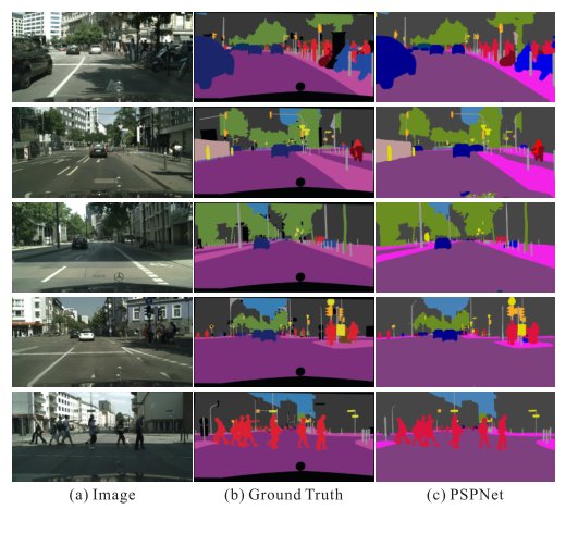
Figure 8: Examples of PSPNet results on Cityscapes dataset.
图 8:Cityscapes 上 PSPNet 结果示例。
5.4 Cityscapes
Cityscapes cordts2016cityscapes is a recently released dataset for semantic urban scene understanding. It contains 5,000 high quality pixel-level finely annotated images collected from 50 cities in different seasons. The images are divided into sets with numbers 2,975, 500, and 1,525 for training, validation and testing. It defines 19 categories containing both stuff and objects. Also, 20,000 coarsely annotated images are provided for two settings in comparison, i.e., training with only fine data or with both the fine and coarse data. Methods trained using both fine and coarse data are marked with ‘’. Detailed results are listed in Table 7. Our base model is ResNet101 as in DeepLab chen2016deeplab for fair comparison and the testing procedure follows Section 5.3.
Cityscapes cordts2016cityscapes 是面向城市语义理解的新发布数据集,含来自 50 座城市、不同季节的 5,000 张高质量像素级精标注图像,划分为训练/验证/测试 2,975、500、1,525 张,定义 19 类 stuff 与物体。另提供 20,000 张粗标注图像,对应「仅 fine」或「fine+coarse」两种训练设定;后者标以 ‘’。详细结果见表 7。骨干为与 DeepLab chen2016deeplab 相同的 ResNet101 以便公平对比,测试流程同第 5.3 节。
Statistics in Table 7 show that PSPNet outperforms other methods with notable advantage. Using both fine and coarse data for training makes our method yield 80.2 accuracy. Several examples are shown in Fig. 8. Detailed per-class results on testing set are shown in Table 8.
表 7 显示 PSPNet 以明显优势超过其他方法;用 fine+coarse 训练时达到 80.2。图 8 给出若干例子;测试集逐类结果见表 8。
6 Concluding Remarks
6 结语
We have proposed an effective pyramid scene parsing network for complex scene understanding. The global pyramid pooling feature provides additional contextual information. We have also provided a deeply supervised optimization strategy for ResNet-based FCN network. We hope the implementation details publicly available can help the community adopt these useful strategies for scene parsing and semantic segmentation and advance related techniques.
我们提出面向复杂场景理解的有效金字塔场景解析网络:全局金字塔池化特征提供额外上下文,并给出面向基于 ResNet 的 FCN 的深度监督优化策略。希望公开的实现细节能帮助社区采用这些策略于场景解析与语义分割,并推动相关技术发展。
Acknowledgements
致谢
We would like to thank Gang Sun and Tong Xiao for their help in training the basic classification models, Qun Luo for technical support. This work is supported by a grant from the Research Grants Council of the Hong Kong SAR (project No. 2150760).
感谢 Gang Sun 与 Tong Xiao 在基础分类模型训练上的帮助,以及 Qun Luo 的技术支持。本研究获香港特别行政区研究资助局资助(项目编号 2150760)。
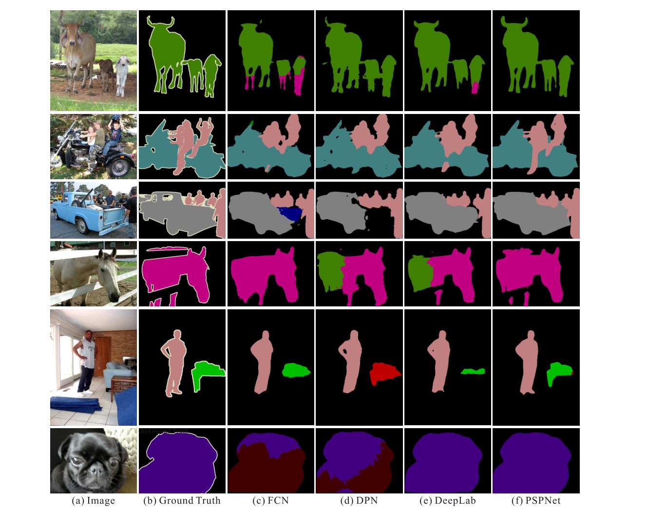
Figure 9: Visual comparison on PASCAL VOC 2012 data. (a) Image. (b) Ground Truth. (c) FCN long2015fully. (d) DPN liu2015parsenet. (e) DeepLab chen2016deeplab. (f) PSPNet.
图 9:PASCAL VOC 2012 上的视觉对比。(a) 图像。(b) 真值。(c) FCN long2015fully。(d) DPN liu2015parsenet。(e) DeepLab chen2016deeplab。(f) PSPNet。
| Method | road | swalk | build. | wall | fence | pole | tlight | sign | veg. | terrain | sky | person | rider | car | truck | bus | train | mbike | bike | mIoU |
|---|---|---|---|---|---|---|---|---|---|---|---|---|---|---|---|---|---|---|---|---|
| CRF-RNN zheng2015conditional | 96.3 | 73.9 | 88.2 | 47.6 | 41.3 | 35.2 | 49.5 | 59.7 | 90.6 | 66.1 | 93.5 | 70.4 | 34.7 | 90.1 | 39.2 | 57.5 | 55.4 | 43.9 | 54.6 | 62.5 |
| FCN long2015fully | 97.4 | 78.4 | 89.2 | 34.9 | 44.2 | 47.4 | 60.1 | 65.0 | 91.4 | 69.3 | 93.9 | 77.1 | 51.4 | 92.6 | 35.3 | 48.6 | 46.5 | 51.6 | 66.8 | 65.3 |
| SiCNN+CRF krevso2016convolutional | 96.3 | 76.8 | 88.8 | 40.0 | 45.4 | 50.1 | 63.3 | 69.6 | 90.6 | 67.1 | 92.2 | 77.6 | 55.9 | 90.1 | 39.2 | 51.3 | 44.4 | 54.4 | 66.1 | 66.3 |
| DPN liu2015semantic | 97.5 | 78.5 | 89.5 | 40.4 | 45.9 | 51.1 | 56.8 | 65.3 | 91.5 | 69.4 | 94.5 | 77.5 | 54.2 | 92.5 | 44.5 | 53.4 | 49.9 | 52.1 | 64.8 | 66.8 |
| Dilation10 yu2015multi | 97.6 | 79.2 | 89.9 | 37.3 | 47.6 | 53.2 | 58.6 | 65.2 | 91.8 | 69.4 | 93.7 | 78.9 | 55.0 | 93.3 | 45.5 | 53.4 | 47.7 | 52.2 | 66.0 | 67.1 |
| LRR ghiasi2016laplacian | 97.7 | 79.9 | 90.7 | 44.4 | 48.6 | 58.6 | 68.2 | 72.0 | 92.5 | 69.3 | 94.7 | 81.6 | 60.0 | 94.0 | 43.6 | 56.8 | 47.2 | 54.8 | 69.7 | 69.7 |
| DeepLab chen2016deeplab | 97.9 | 81.3 | 90.3 | 48.8 | 47.4 | 49.6 | 57.9 | 67.3 | 91.9 | 69.4 | 94.2 | 79.8 | 59.8 | 93.7 | 56.5 | 67.5 | 57.5 | 57.7 | 68.8 | 70.4 |
| Piecewise lin2015efficient | 98.0 | 82.6 | 90.6 | 44.0 | 50.7 | 51.1 | 65.0 | 71.7 | 92.0 | 72.0 | 94.1 | 81.5 | 61.1 | 94.3 | 61.1 | 65.1 | 53.8 | 61.6 | 70.6 | 71.6 |
| PSPNet | 98.6 | 86.2 | 92.9 | 50.8 | 58.8 | 64.0 | 75.6 | 79.0 | 93.4 | 72.3 | 95.4 | 86.5 | 71.3 | 95.9 | 68.2 | 79.5 | 73.8 | 69.5 | 77.2 | 78.4 |
| LRR*‡* ghiasi2016laplacian | 97.9 | 81.5 | 91.4 | 50.5 | 52.7 | 59.4 | 66.8 | 72.7 | 92.5 | 70.1 | 95.0 | 81.3 | 60.1 | 94.3 | 51.2 | 67.7 | 54.6 | 55.6 | 69.6 | 71.8 |
| PSPNet*‡* | 98.6 | 86.6 | 93.2 | 58.1 | 63.0 | 64.5 | 75.2 | 79.2 | 93.4 | 72.1 | 95.1 | 86.3 | 71.4 | 96.0 | 73.5 | 90.4 | 80.3 | 69.9 | 76.9 | 80.2 |
Table 8: Per-class results on Cityscapes testing set. Methods trained using both fine and coarse set are marked with ‘’.
| 方法 | road | swalk | build. | wall | fence | pole | tlight | sign | veg. | terrain | sky | person | rider | car | truck | bus | train | mbike | bike | mIoU |
|---|---|---|---|---|---|---|---|---|---|---|---|---|---|---|---|---|---|---|---|---|
| CRF-RNN zheng2015conditional | 96.3 | 73.9 | 88.2 | 47.6 | 41.3 | 35.2 | 49.5 | 59.7 | 90.6 | 66.1 | 93.5 | 70.4 | 34.7 | 90.1 | 39.2 | 57.5 | 55.4 | 43.9 | 54.6 | 62.5 |
| FCN long2015fully | 97.4 | 78.4 | 89.2 | 34.9 | 44.2 | 47.4 | 60.1 | 65.0 | 91.4 | 69.3 | 93.9 | 77.1 | 51.4 | 92.6 | 35.3 | 48.6 | 46.5 | 51.6 | 66.8 | 65.3 |
| SiCNN+CRF krevso2016convolutional | 96.3 | 76.8 | 88.8 | 40.0 | 45.4 | 50.1 | 63.3 | 69.6 | 90.6 | 67.1 | 92.2 | 77.6 | 55.9 | 90.1 | 39.2 | 51.3 | 44.4 | 54.4 | 66.1 | 66.3 |
| DPN liu2015semantic | 97.5 | 78.5 | 89.5 | 40.4 | 45.9 | 51.1 | 56.8 | 65.3 | 91.5 | 69.4 | 94.5 | 77.5 | 54.2 | 92.5 | 44.5 | 53.4 | 49.9 | 52.1 | 64.8 | 66.8 |
| Dilation10 yu2015multi | 97.6 | 79.2 | 89.9 | 37.3 | 47.6 | 53.2 | 58.6 | 65.2 | 91.8 | 69.4 | 93.7 | 78.9 | 55.0 | 93.3 | 45.5 | 53.4 | 47.7 | 52.2 | 66.0 | 67.1 |
| LRR ghiasi2016laplacian | 97.7 | 79.9 | 90.7 | 44.4 | 48.6 | 58.6 | 68.2 | 72.0 | 92.5 | 69.3 | 94.7 | 81.6 | 60.0 | 94.0 | 43.6 | 56.8 | 47.2 | 54.8 | 69.7 | 69.7 |
| DeepLab chen2016deeplab | 97.9 | 81.3 | 90.3 | 48.8 | 47.4 | 49.6 | 57.9 | 67.3 | 91.9 | 69.4 | 94.2 | 79.8 | 59.8 | 93.7 | 56.5 | 67.5 | 57.5 | 57.7 | 68.8 | 70.4 |
| Piecewise lin2015efficient | 98.0 | 82.6 | 90.6 | 44.0 | 50.7 | 51.1 | 65.0 | 71.7 | 92.0 | 72.0 | 94.1 | 81.5 | 61.1 | 94.3 | 61.1 | 65.1 | 53.8 | 61.6 | 70.6 | 71.6 |
| PSPNet | 98.6 | 86.2 | 92.9 | 50.8 | 58.8 | 64.0 | 75.6 | 79.0 | 93.4 | 72.3 | 95.4 | 86.5 | 71.3 | 95.9 | 68.2 | 79.5 | 73.8 | 69.5 | 77.2 | 78.4 |
| LRR*‡* ghiasi2016laplacian | 97.9 | 81.5 | 91.4 | 50.5 | 52.7 | 59.4 | 66.8 | 72.7 | 92.5 | 70.1 | 95.0 | 81.3 | 60.1 | 94.3 | 51.2 | 67.7 | 54.6 | 55.6 | 69.6 | 71.8 |
| PSPNet*‡* | 98.6 | 86.6 | 93.2 | 58.1 | 63.0 | 64.5 | 75.2 | 79.2 | 93.4 | 72.1 | 95.1 | 86.3 | 71.4 | 96.0 | 73.5 | 90.4 | 80.3 | 69.9 | 76.9 | 80.2 |
表 8:Cityscapes 测试集逐类结果。同时用 fine 与 coarse 集训练的方法标以 ‘’。
References
参考文献
(1) A. Arnab, S. Jayasumana, S. Zheng, and P. H. S. Torr. Higher order conditional random fields in deep neural networks. In ECCV , 2016.
(2) V. Badrinarayanan, A. Kendall, and R. Cipolla. Segnet: A deep convolutional encoder-decoder architecture for image segmentation. arXiv:1511.00561 , 2015.
(3) L. Chen, G. Papandreou, I. Kokkinos, K. Murphy, and A. L. Yuille. Semantic image segmentation with deep convolutional nets and fully connected crfs. arXiv:1412.7062 , 2014.
(4) L. Chen, G. Papandreou, I. Kokkinos, K. Murphy, and A. L. Yuille. Deeplab: Semantic image segmentation with deep convolutional nets, atrous convolution, and fully connected crfs. arXiv:1606.00915 , 2016.
(5) L. Chen, Y. Yang, J. Wang, W. Xu, and A. L. Yuille. Attention to scale: Scale-aware semantic image segmentation. In CVPR , 2016.
(6) M. Cordts, M. Omran, S. Ramos, T. Rehfeld, M. Enzweiler, R. Benenson, U. Franke, S. Roth, and B. Schiele. The cityscapes dataset for semantic urban scene understanding. In CVPR , 2016.
(7) J. Dai, K. He, and J. Sun. Boxsup: Exploiting bounding boxes to supervise convolutional networks for semantic segmentation. In ICCV , 2015.
(8) M. Everingham, L. J. V. Gool, C. K. I. Williams, J. M. Winn, and A. Zisserman. The pascal visual object classes VOC challenge. IJCV , 2010.
(9) G. Ghiasi and C. C. Fowlkes. Laplacian pyramid reconstruction and refinement for semantic segmentation. In ECCV , 2016.
(10) B. Hariharan, P. Arbelaez, L. D. Bourdev, S. Maji, and J. Malik. Semantic contours from inverse detectors. In ICCV , 2011.
(11) B. Hariharan, P. A. Arbeláez, R. B. Girshick, and J. Malik. Hypercolumns for object segmentation and fine-grained localization. In CVPR , 2015.
(12) K. He, X. Zhang, S. Ren, and J. Sun. Spatial pyramid pooling in deep convolutional networks for visual recognition. In ECCV , 2014.
(13) K. He, X. Zhang, S. Ren, and J. Sun. Deep residual learning for image recognition. In CVPR , 2016.
(14) S. Ioffe and C. Szegedy. Batch normalization: Accelerating deep network training by reducing internal covariate shift. In ICML , 2015.
(15) Y. Jia, E. Shelhamer, J. Donahue, S. Karayev, J. Long, R. B. Girshick, S. Guadarrama, and T. Darrell. Caffe: Convolutional architecture for fast feature embedding. In ACM MM , 2014.
(16) I. Kreso, D. Causevic, J. Krapac, and S. Segvic. Convolutional scale invariance for semantic segmentation. In GCPR , 2016.
(17) A. Krizhevsky, I. Sutskever, and G. E. Hinton. Imagenet classification with deep convolutional neural networks. In NIPS , 2012.
(18) S. Lazebnik, C. Schmid, and J. Ponce. Beyond bags of features: Spatial pyramid matching for recognizing natural scene categories. In CVPR , 2006.
(19) C. Lee, S. Xie, P. W. Gallagher, Z. Zhang, and Z. Tu. Deeply-supervised nets. In AISTATS , 2015.
(20) G. Lin, C. Shen, I. D. Reid, and A. van den Hengel. Efficient piecewise training of deep structured models for semantic segmentation. In CVPR , 2016.
(21) T. Lin, M. Maire, S. J. Belongie, J. Hays, P. Perona, D. Ramanan, P. Dollár, and C. L. Zitnick. Microsoft coco: Common objects in context. In ECCV , 2014.
(22) C. Liu, J. Yuen, and A. Torralba. Nonparametric scene parsing: Label transfer via dense scene alignment. In CVPR , 2009.
(23) C. Liu, J. Yuen, and A. Torralba. Nonparametric scene parsing via label transfer. TPAMI , 2011.
(24) W. Liu, A. Rabinovich, and A. C. Berg. Parsenet: Looking wider to see better. arXiv:1506.04579 , 2015.
(25) Z. Liu, X. Li, P. Luo, C. C. Loy, and X. Tang. Semantic image segmentation via deep parsing network. In ICCV , 2015.
(26) J. Long, E. Shelhamer, and T. Darrell. Fully convolutional networks for semantic segmentation. In CVPR , 2015.
(27) A. Lucchi, Y. Li, X. B. Bosch, K. Smith, and P. Fua. Are spatial and global constraints really necessary for segmentation? In ICCV , 2011.
(28) M. Mostajabi, P. Yadollahpour, and G. Shakhnarovich. Feedforward semantic segmentation with zoom-out features. In CVPR , 2015.
(29) R. Mottaghi, X. Chen, X. Liu, N. Cho, S. Lee, S. Fidler, R. Urtasun, and A. L. Yuille. The role of context for object detection and semantic segmentation in the wild. In CVPR , 2014.
(30) H. Noh, S. Hong, and B. Han. Learning deconvolution network for semantic segmentation. In ICCV , 2015.
(31) G. Papandreou, L. Chen, K. P. Murphy, and A. L. Yuille. Weakly-and semi-supervised learning of a deep convolutional network for semantic image segmentation. In ICCV , 2015.
(32) L. Shen, Z. Lin, and Q. Huang. Relay backpropagation for effective learning of deep convolutional neural networks. In ECCV , 2016.
(33) K. Simonyan and A. Zisserman. Very deep convolutional networks for large-scale image recognition. arXiv:1409.1556 , 2014.
(34) C. Szegedy, W. Liu, Y. Jia, P. Sermanet, S. E. Reed, D. Anguelov, D. Erhan, V. Vanhoucke, and A. Rabinovich. Going deeper with convolutions. In CVPR , 2015.
(35) C. Szegedy, S. E. Reed, D. Erhan, and D. Anguelov. Scalable, high-quality object detection. arXiv:1412.1441 , 2014.
(36) R. Vemulapalli, O. Tuzel, M. Liu, and R. Chellappa. Gaussian conditional random field network for semantic segmentation. In CVPR , 2016.
(37) L. Wang, Y. Xiong, Z. Wang, and Y. Qiao. Towards good practices for very deep two-stream convnets. arXiv:1507.02159 , 2015.
(38) Z. Wu, C. Shen, and A. van den Hengel. Bridging category-level and instance-level semantic image segmentation. arXiv:1605.06885 , 2016.
(39) F. Xia, P. Wang, L. Chen, and A. L. Yuille. Zoom better to see clearer: Human and object parsing with hierarchical auto-zoom net. In ECCV , 2016.
(40) F. Yu and V. Koltun. Multi-scale context aggregation by dilated convolutions. arXiv:1511.07122 , 2015.
(41) S. Zheng, S. Jayasumana, B. Romera-Paredes, V. Vineet, Z. Su, D. Du, C. Huang, and P. H. S. Torr. Conditional random fields as recurrent neural networks. In ICCV , 2015.
(42) B. Zhou, A. Khosla, À. Lapedriza, A. Oliva, and A. Torralba. Object detectors emerge in deep scene cnns. arXiv:1412.6856 , 2014.
(43) B. Zhou, H. Zhao, X. Puig, S. Fidler, A. Barriuso, and A. Torralba. Semantic understanding of scenes through the ADE20K dataset. arXiv:1608.05442 , 2016.