Prototypical Networks for Few-shot Learning

用于小样本学习的原型网络

Jake Snell Affiliation:  University of Toronto    Kevin Swersky Affiliation:  Twitter    Richard S. Zemel Affiliation:  University of Toronto, Vector Institute

Abstract

摘要

We propose prototypical networks for the problem of few-shot classification, where a classifier must generalize to new classes not seen in the training set, given only a small number of examples of each new class. Prototypical networks learn a metric space in which classification can be performed by computing distances to prototype representations of each class. Compared to recent approaches for few-shot learning, they reflect a simpler inductive bias that is beneficial in this limited-data regime, and achieve excellent results. We provide an analysis showing that some simple design decisions can yield substantial improvements over recent approaches involving complicated architectural choices and meta-learning. We further extend prototypical networks to zero-shot learning and achieve state-of-the-art results on the CU-Birds dataset.

我们提出原型网络（prototypical networks），用于小样本分类：分类器必须在训练集中从未见过的新类别上泛化，而每个新类只有少量样本。原型网络学习一个度量空间，分类只需计算到各类原型表示的距离。与近期的小样本学习方法相比，它体现了一种更简单、在数据极少时反而有益的归纳偏置，并取得了出色的结果。我们通过分析表明，一些简单的设计选择就能相对近来那些结构复杂、依赖元学习的方法带来显著改进。我们还把原型网络推广到零样本学习，并在 CU-Birds 数据集上取得了当时最好的结果。

1 Introduction

1 引言

Few-shot classification [20, 16, 13] is a task in which a classifier must be adapted to accommodate new classes not seen in training, given only a few examples of each of these classes. A naive approach, such as re-training the model on the new data, would severely overfit. While the problem is quite difficult, it has been demonstrated that humans have the ability to perform even one-shot classification, where only a single example of each new class is given, with a high degree of accuracy [16].

小样本分类 [20, 16, 13] 要求分类器适应训练时未见过的新类别，而每个新类只有少量样本。若简单地在新数据上重新训练模型，会严重过拟合。这个问题虽然很难，但已有研究表明，人类即使在一类只有一个样本的单样本分类中，也能达到很高的准确率 [16]。

Two recent approaches have made significant progress in few-shot learning. Vinyals et al. [29] proposed matching networks, which uses an attention mechanism over a learned embedding of the labeled set of examples (the support set) to predict classes for the unlabeled points (the query set). Matching networks can be interpreted as a weighted nearest-neighbor classifier applied within an embedding space. Notably, this model utilizes sampled mini-batches called episodes during training, where each episode is designed to mimic the few-shot task by subsampling classes as well as data points. The use of episodes makes the training problem more faithful to the test environment and thereby improves generalization. Ravi and Larochelle [22] take the episodic training idea further and propose a meta-learning approach to few-shot learning. Their approach involves training an LSTM [9] to produce the updates to a classifier, given an episode, such that it will generalize well to a test-set. Here, rather than training a single model over multiple episodes, the LSTM meta-learner learns to train a custom model for each episode.

近期有两条路径在小样本学习上取得了显著进展。Vinyals 等 [29] 提出匹配网络（matching networks），在一组带标签样本（支持集）的学得嵌入上使用注意力机制，来预测未标注点（查询集）的类别。匹配网络可以理解为嵌入空间中的加权最近邻分类器。该模型在训练时使用称为回合（episode）的采样小批次：每个回合通过子采样类别和数据点来模拟小样本任务。回合使训练问题更接近测试环境，从而改善泛化。Ravi 与 Larochelle [22] 把回合训练的想法推得更远，提出一种用于小样本学习的元学习方法。他们训练一个 LSTM [9]，根据一个回合来生成分类器的更新，使其能在测试集上泛化得更好。这里不是在多个回合上训练同一个模型，而是让 LSTM 元学习器学会为每个回合训练一个定制模型。

We attack the problem of few-shot learning by addressing the key issue of overfitting. Since data is severely limited, we work under the assumption that a classifier should have a very simple inductive bias. Our approach, prototypical networks, is based on the idea that there exists an embedding in which points cluster around a single prototype representation for each class. In order to do this, we learn a non-linear mapping of the input into an embedding space using a neural network and take a class’s prototype to be the mean of its support set in the embedding space. Classification is then performed for an embedded query point by simply finding the nearest class prototype. We follow the same approach to tackle zero-shot learning; here each class comes with meta-data giving a high-level description of the class rather than a small number of labeled examples. We therefore learn an embedding of the meta-data into a shared space to serve as the prototype for each class. Classification is performed, as in the few-shot scenario, by finding the nearest class prototype for an embedded query point.

我们从过拟合这一核心问题入手来做小样本学习。既然数据极度有限，我们假定分类器应当具有非常简单的归纳偏置。我们的方法——原型网络——基于这样的想法：存在一种嵌入，使各类样本聚集在该类的单一原型表示周围。为此，我们用神经网络学习从输入到嵌入空间的非线性映射，并把一类的原型取作其支持集在嵌入空间中的均值。对一个嵌入后的查询点，分类只需找到最近的类原型。我们用同样的思路处理零样本学习：此时每个类带有元数据，给出该类的高层描述，而不是少量带标签样本。于是我们学习把元数据嵌入到同一共享空间，作为每个类的原型。分类方式与小样本情形相同：为嵌入后的查询点寻找最近的类原型。

In this paper, we formulate prototypical networks for both the few-shot and zero-shot settings. We draw connections to matching networks in the one-shot setting, and analyze the underlying distance function used in the model. In particular, we relate prototypical networks to clustering [4] in order to justify the use of class means as prototypes when distances are computed with a Bregman divergence, such as squared Euclidean distance. We find empirically that the choice of distance is vital, as Euclidean distance greatly outperforms the more commonly used cosine similarity. On several benchmark tasks, we achieve state-of-the-art performance. Prototypical networks are simpler and more efficient than recent meta-learning algorithms, making them an appealing approach to few-shot and zero-shot learning.

本文分别给出小样本和零样本设定下的原型网络。我们在单样本情形下把它与匹配网络联系起来，并分析模型所用的距离函数。特别地，我们把原型网络与聚类 [4] 联系起来，以说明：当距离是 Bregman 散度（例如平方欧氏距离）时，用类均值作为原型是合理的。实验发现距离的选择至关重要，欧氏距离大幅优于更常用的余弦相似度。在多个基准任务上，我们取得了当时最好的结果。原型网络比近期的元学习算法更简单、也更高效，因而是小样本和零样本学习中有吸引力的一条路径。

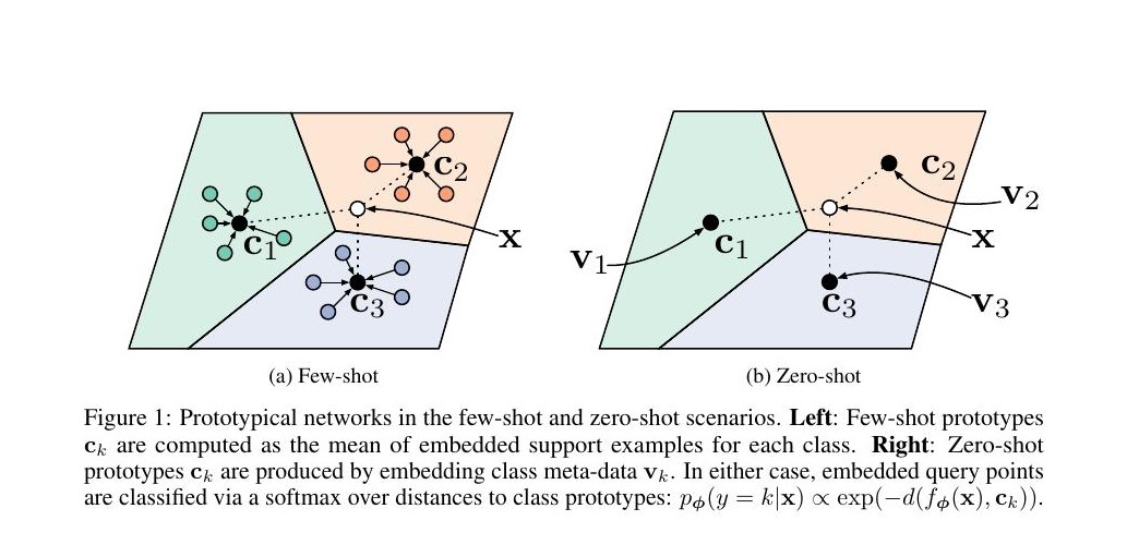
Figure 1: Prototypical networks in the few-shot and zero-shot scenarios. Left: Few-shot prototypes $\mathbf{c}_{k}$ are computed as the mean of embedded support examples for each class. Right: Zero-shot prototypes $\mathbf{c}_{k}$ are produced by embedding class meta-data $\mathbf{v}_{k}$. In either case, embedded query points are classified via a softmax over distances to class prototypes: $p_{\bm{\phi}}(y=k\,|\,\mathbf{x})\propto\exp(-d(f_{\bm{\phi}}(\mathbf{x}),\mathbf{c}_{k}))$.

图 1：原型网络在小样本与零样本设定下的示意。左：小样本原型 $\mathbf{c}_{k}$ 取作各类嵌入后支持样本的均值。右：零样本原型 $\mathbf{c}_{k}$ 由嵌入类元数据 $\mathbf{v}_{k}$ 得到。两种情形下，嵌入后的查询点都通过对到各类原型的距离做 softmax 来分类：$p_{\bm{\phi}}(y=k\,|\,\mathbf{x})\propto\exp(-d(f_{\bm{\phi}}(\mathbf{x}),\mathbf{c}_{k}))$。

2 Prototypical Networks

2 原型网络

2.1 Notation

2.1 记号

In few-shot classification we are given a small support set of $N$ labeled examples $S=\{(\mathbf{x}_{1},y_{1}),\ldots,(\mathbf{x}_{N},y_{N})\}$ where each $\mathbf{x}_{i}\in\mathbb{R}^{D}$ is the $D$-dimensional feature vector of an example and $y_{i}\in\{1,\ldots,K\}$ is the corresponding label. $S_{k}$ denotes the set of examples labeled with class $k$.

在小样本分类中，我们得到一个由 $N$ 个带标签样本组成的小支持集 $S=\{(\mathbf{x}_{1},y_{1}),\ldots,(\mathbf{x}_{N},y_{N})\}$，其中每个 $\mathbf{x}_{i}\in\mathbb{R}^{D}$ 是样本的 $D$ 维特征向量，$y_{i}\in\{1,\ldots,K\}$ 是对应标签。$S_{k}$ 表示标签为类别 $k$ 的样本集合。

2.2 Model

2.2 模型

Prototypical networks compute an $M$-dimensional representation $\mathbf{c}_{k}\in\mathbb{R}^{M}$, or prototype, of each class through an embedding function $f_{\bm{\phi}}:\mathbb{R}^{D}\rightarrow\mathbb{R}^{M}$ with learnable parameters $\bm{\phi}$. Each prototype is the mean vector of the embedded support points belonging to its class:

原型网络通过带可学习参数 $\bm{\phi}$ 的嵌入函数 $f_{\bm{\phi}}:\mathbb{R}^{D}\rightarrow\mathbb{R}^{M}$，为每个类计算一个 $M$ 维表示 $\mathbf{c}_{k}\in\mathbb{R}^{M}$，也就是原型。每个原型是属于该类的嵌入支持点的均值向量：

$$\mathbf{c}_{k}=\frac{1}{|S_{k}|}\sum_{(\mathbf{x}_{i},y_{i})\in S_{k}}f_{\bm{\phi}}(\mathbf{x}_{i}) \tag{1}$$

Given a distance function $d:\mathbb{R}^{M}\times\mathbb{R}^{M}\rightarrow[0,+\infty)$, prototypical networks produce a distribution over classes for a query point $\mathbf{x}$ based on a softmax over distances to the prototypes in the embedding space:

给定距离函数 $d:\mathbb{R}^{M}\times\mathbb{R}^{M}\rightarrow[0,+\infty)$，原型网络根据查询点 $\mathbf{x}$ 到各原型在嵌入空间中的距离，经 softmax 得到类别分布：

$$p_{\bm{\phi}}(y=k\,|\,\mathbf{x})=\frac{\exp(-d(f_{\bm{\phi}}(\mathbf{x}),\mathbf{c}_{k}))}{\sum_{k^{\prime}}\exp(-d(f_{\bm{\phi}}(\mathbf{x}),\mathbf{c}_{k^{\prime}}))} \tag{2}$$

Learning proceeds by minimizing the negative log-probability $J(\bm{\phi})=-\log p_{\bm{\phi}}(y=k\,|\,\mathbf{x})$ of the true class $k$ via SGD. Training episodes are formed by randomly selecting a subset of classes from the training set, then choosing a subset of examples within each class to act as the support set and a subset of the remainder to serve as query points. Pseudocode to compute the loss $J(\bm{\phi})$ for a training episode is provided in Algorithm 1.

学习通过 SGD 最小化真实类别 $k$ 的负对数概率 $J(\bm{\phi})=-\log p_{\bm{\phi}}(y=k\,|\,\mathbf{x})$。构成训练回合的方式是：先从训练集中随机选出一部分类别，再在每个类中选出一部分样本作为支持集，其余中再选出一部分作为查询点。计算一个训练回合损失 $J(\bm{\phi})$ 的伪代码见算法 1。

0:  Training set $\mathcal{D}=\{(\mathbf{x}_{1},y_{1}),\ldots,(\mathbf{x}_{N},y_{N})\}$, where each $y_{i}\in\{1,\ldots,K\}$. $\mathcal{D}_{k}$ denotes the subset of $\mathcal{D}$ containing all elements $(\mathbf{x}_{i},y_{i})$ such that $y_{i}=k$.
0:  The loss $J$ for a randomly generated training episode.
$V\leftarrow\textsc{RandomSample}(\{1,\ldots,K\},N_{C})$ $\triangleright$ Select class indices for episode
for $k$ in $\{1,\ldots,N_{C}\}$ do
$S_{k}\leftarrow\textsc{RandomSample}(\mathcal{D}_{V_{k}},N_{S})$ $\triangleright$ Select support examples
$Q_{k}\leftarrow\textsc{RandomSample}(\mathcal{D}_{V_{k}}\setminus S_{k},N_{Q})$ $\triangleright$ Select query examples
$\displaystyle\mathbf{c}_{k}\leftarrow\frac{1}{N_{C}}\sum_{(\mathbf{x}_{i},y_{i})\in S_{k}}f_{\bm{\phi}}(\mathbf{x}_{i})$ $\triangleright$ Compute prototype from support examples
end for
$J\leftarrow 0$ $\triangleright$ Initialize loss
for $k$ in $\{1,\ldots,N_{C}\}$ do
for $(\mathbf{x},y)$ in $Q_{k}$ do
$\displaystyle J\leftarrow J+\frac{1}{N_{C}N_{Q}}\left[d(f_{\bm{\phi}}(\mathbf{x}),\mathbf{c}_{k}))+\log\sum_{k^{\prime}}\exp(-d(f_{\bm{\phi}}(\mathbf{x}),\mathbf{c}_{k}))\right]$ $\triangleright$ Update loss
end for
end for

Algorithm 1 Training episode loss computation for prototypical networks. $N$ is the number of examples in the training set, $K$ is the number of classes in the training set, $N_{C}\leq K$ is the number of classes per episode, $N_{S}$ is the number of support examples per class, $N_{Q}$ is the number of query examples per class. $\textsc{RandomSample}(S,N)$ denotes a set of $N$ elements chosen uniformly at random from set $S$, without replacement.

0:  训练集 $\mathcal{D}=\{(\mathbf{x}_{1},y_{1}),\ldots,(\mathbf{x}_{N},y_{N})\}$，其中每个 $y_{i}\in\{1,\ldots,K\}$。$\mathcal{D}_{k}$ 表示 $\mathcal{D}$ 中所有满足 $y_{i}=k$ 的元素 $(\mathbf{x}_{i},y_{i})$ 组成的子集。
0:  一个随机生成的训练回合的损失 $J$。
$V\leftarrow\textsc{RandomSample}(\{1,\ldots,K\},N_{C})$ $\triangleright$ 为本回合选择类别下标
for $k$ in $\{1,\ldots,N_{C}\}$ do
$S_{k}\leftarrow\textsc{RandomSample}(\mathcal{D}_{V_{k}},N_{S})$ $\triangleright$ 选择支持样本
$Q_{k}\leftarrow\textsc{RandomSample}(\mathcal{D}_{V_{k}}\setminus S_{k},N_{Q})$ $\triangleright$ 选择查询样本
$\displaystyle\mathbf{c}_{k}\leftarrow\frac{1}{N_{C}}\sum_{(\mathbf{x}_{i},y_{i})\in S_{k}}f_{\bm{\phi}}(\mathbf{x}_{i})$ $\triangleright$ 由支持样本计算原型
end for
$J\leftarrow 0$ $\triangleright$ 初始化损失
for $k$ in $\{1,\ldots,N_{C}\}$ do
for $(\mathbf{x},y)$ in $Q_{k}$ do
$\displaystyle J\leftarrow J+\frac{1}{N_{C}N_{Q}}\left[d(f_{\bm{\phi}}(\mathbf{x}),\mathbf{c}_{k}))+\log\sum_{k^{\prime}}\exp(-d(f_{\bm{\phi}}(\mathbf{x}),\mathbf{c}_{k}))\right]$ $\triangleright$ 更新损失
end for
end for

算法 1 原型网络一个训练回合的损失计算。$N$ 是训练集中的样本数，$K$ 是训练集中的类别数，$N_{C}\leq K$ 是每个回合的类别数，$N_{S}$ 是每类的支持样本数，$N_{Q}$ 是每类的查询样本数。$\textsc{RandomSample}(S,N)$ 表示从集合 $S$ 中无放回地均匀随机取出 $N$ 个元素。

2.3 Prototypical Networks as Mixture Density Estimation

2.3 作为混合密度估计的原型网络

For a particular class of distance functions, known as regular Bregman divergences [4], the prototypical networks algorithm is equivalent to performing mixture density estimation on the support set with an exponential family density. A regular Bregman divergence $d_{\varphi}$ is defined as:

对一类称为正则 Bregman 散度 [4] 的距离函数，原型网络算法等价于在支持集上用指数族密度做混合密度估计。正则 Bregman 散度 $d_{\varphi}$ 定义为：

$$d_{\varphi}(\mathbf{z},\mathbf{z}^{\prime})=\varphi(\mathbf{z})-\varphi(\mathbf{z}^{\prime})-(\mathbf{z}-\mathbf{z}^{\prime})^{T}\nabla\varphi(\mathbf{z}^{\prime}), \tag{3}$$

where $\varphi$ is a differentiable, strictly convex function of the Legendre type. Examples of Bregman divergences include squared Euclidean distance $\|\mathbf{z}-\mathbf{z}^{\prime}\|^{2}$ and Mahalanobis distance.

其中 $\varphi$ 是 Legendre 型的可微严格凸函数。Bregman 散度的例子包括平方欧氏距离 $\|\mathbf{z}-\mathbf{z}^{\prime}\|^{2}$ 以及马氏距离。

Prototype computation can be viewed in terms of hard clustering on the support set, with one cluster per class and each support point assigned to its corresponding class cluster. It has been shown [4] for Bregman divergences that the cluster representative achieving minimal distance to its assigned points is the cluster mean. Thus the prototype computation in Equation (1) yields optimal cluster representatives given the support set labels when a Bregman divergence is used.

原型的计算可以看成支持集上的硬聚类：每个类一个簇，每个支持点被分到对应的类簇。已经证明 [4]，对 Bregman 散度，使到所分配点距离最小的簇代表就是簇均值。因此，当使用 Bregman 散度时，公式 (1) 中的原型计算在给定支持集标签下给出了最优的簇代表。

Moreover, any regular exponential family distribution $p_{\psi}(\mathbf{z}|\bm{\theta})$ with parameters $\bm{\theta}$ and cumulant function $\psi$ can be written in terms of a uniquely determined regular Bregman divergence [4]:

此外，任何带参数 $\bm{\theta}$ 和累积量函数 $\psi$ 的正则指数族分布 $p_{\psi}(\mathbf{z}|\bm{\theta})$，都可以写成由它唯一确定的正则 Bregman 散度的形式 [4]：

$$p_{\psi}(\mathbf{z}|\bm{\theta})=\exp\{\mathbf{z}^{T}\bm{\theta}-\psi(\bm{\theta})-g_{\psi}(\mathbf{z})\}=\exp\{-d_{\varphi}(\mathbf{z},\bm{\mu}(\bm{\theta}))-g_{\varphi}(\mathbf{z})\} \tag{4}$$

Consider now a regular exponential family mixture model with parameters $\bm{\Gamma}=\{\bm{\theta}_{k},\pi_{k}\}_{k=1}^{K}$:

现在考虑参数为 $\bm{\Gamma}=\{\bm{\theta}_{k},\pi_{k}\}_{k=1}^{K}$ 的正则指数族混合模型：

$$p(\mathbf{z}|\bm{\Gamma})=\sum_{k=1}^{K}\pi_{k}p_{\psi}(\mathbf{z}|\bm{\theta}_{k})=\sum_{k=1}^{K}\pi_{k}\exp(-d_{\varphi}(\mathbf{z},\bm{\mu}(\bm{\theta}_{k}))-g_{\varphi}(\mathbf{z})) \tag{5}$$

Given $\bm{\Gamma}$, inference of the cluster assignment $y$ for an unlabeled point $\mathbf{z}$ becomes:

给定 $\bm{\Gamma}$，对未标注点 $\mathbf{z}$ 推断簇分配 $y$ 变为：

$$p(y=k|\mathbf{z})=\frac{\pi_{k}\exp(-d_{\varphi}(\mathbf{z},\bm{\mu}(\bm{\theta}_{k})))}{\sum_{k^{\prime}}\pi_{k^{\prime}}\exp(-d_{\varphi}(\mathbf{z},\bm{\mu}(\bm{\theta}_{k})))} \tag{6}$$

For an equally-weighted mixture model with one cluster per class, cluster assignment inference (6) is equivalent to query class prediction (2) with $f_{\phi}(\mathbf{x})=\mathbf{z}$ and $\mathbf{c}_{k}=\bm{\mu}(\bm{\theta}_{k})$. In this case, prototypical networks are effectively performing mixture density estimation with an exponential family distribution determined by $d_{\varphi}$. The choice of distance therefore specifies modeling assumptions about the class-conditional data distribution in the embedding space.

对每个类一个簇、且权重相等的混合模型，簇分配推断 (6) 等价于查询点的类别预测 (2)，其中 $f_{\phi}(\mathbf{x})=\mathbf{z}$ 且 $\mathbf{c}_{k}=\bm{\mu}(\bm{\theta}_{k})$。此时，原型网络实际上是在用由 $d_{\varphi}$ 决定的指数族分布做混合密度估计。因此，距离的选择规定了嵌入空间中类条件数据分布的建模假设。

2.4 Reinterpretation as a Linear Model

2.4 重新解释为线性模型

A simple analysis is useful in gaining insight into the nature of the learned classifier. When we use Euclidean distance $d(\mathbf{z},\mathbf{z^{\prime}})=\|\mathbf{z}-\mathbf{z}^{\prime}\|^{2}$, then the model in Equation (2) is equivalent to a linear model with a particular parameterization [19]. To see this, expand the term in the exponent:

一个简单分析有助于理解所学分类器的性质。当使用欧氏距离 $d(\mathbf{z},\mathbf{z^{\prime}})=\|\mathbf{z}-\mathbf{z}^{\prime}\|^{2}$ 时，公式 (2) 中的模型等价于一种特定参数化的线性模型 [19]。为此，把指数中的项展开：

$$\displaystyle-\|f_{\bm{\phi}}(\mathbf{x})-\mathbf{c}_{k}\|^{2} \\ \displaystyle=-f_{\bm{\phi}}(\mathbf{x})^{\top}f_{\bm{\phi}}(\mathbf{x})+2\mathbf{c}_{k}^{\top}f_{\bm{\phi}}(\mathbf{x})-\mathbf{c}_{k}^{\top}\mathbf{c}_{k} \tag{7}$$

The first term in Equation (7) is constant with respect to the class $k$, so it does not affect the softmax probabilities. We can write the remaining terms as a linear model as follows:

公式 (7) 中的第一项相对类别 $k$ 是常数，因而不影响 softmax 概率。其余项可以写成如下线性模型：

$$2\mathbf{c}_{k}^{\top}f_{\bm{\phi}}(\mathbf{x})-\mathbf{c}_{k}^{\top}\mathbf{c}_{k}=\mathbf{w}_{k}^{\top}f_{\bm{\phi}}(\mathbf{x})+b_{k}\mbox{, where }\mathbf{w}_{k}=2\mathbf{c}_{k}\mbox{ and }b_{k}=-\mathbf{c}_{k}^{\top}\mathbf{c}_{k} \tag{8}$$

We focus primarily on squared Euclidean distance (corresponding to spherical Gaussian densities) in this work. Our results indicate that Euclidean distance is an effective choice despite the equivalence to a linear model. We hypothesize this is because all of the required non-linearity can be learned within the embedding function. Indeed, this is the approach that modern neural network classification systems currently use, e.g., [14, 28].

本工作主要关注平方欧氏距离（对应球形高斯密度）。结果表明，尽管它等价于线性模型，欧氏距离仍是有效的选择。我们推测，这是因为所需的非线性都可以在嵌入函数内部学会。事实上，这正是现代神经网络分类系统目前采用的做法，例如 [14, 28]。

2.5 Comparison to Matching Networks

2.5 与匹配网络的比较

Prototypical networks differ from matching networks in the few-shot case with equivalence in the one-shot scenario. Matching networks [29] produce a weighted nearest neighbor classifier given the support set, while prototypical networks produce a linear classifier when squared Euclidean distance is used. In the case of one-shot learning, $\mathbf{c}_{k}=\mathbf{x}_{k}$ since there is only one support point per class, and matching networks and prototypical networks become equivalent.

在小样本情形下，原型网络与匹配网络并不相同；在单样本情形下二者等价。匹配网络 [29] 在给定支持集后产生一个加权最近邻分类器，而原型网络在使用平方欧氏距离时产生一个线性分类器。在单样本学习中，每类只有一个支持点，因而 $\mathbf{c}_{k}=\mathbf{x}_{k}$，匹配网络与原型网络变得等价。

A natural question is whether it makes sense to use multiple prototypes per class instead of just one. If the number of prototypes per class is fixed and greater than $1$, then this would require a partitioning scheme to further cluster the support points within a class. This has been proposed in Mensink et al. [19] and Rippel et al. [25]; however both methods require a separate partitioning phase that is decoupled from the weight updates, while our approach is simple to learn with ordinary gradient descent methods.

一个自然的问题是：每类使用多个原型而不是一个，是否合理。如果每类原型数固定且大于 $1$，就需要一种划分方案，在类内进一步聚类支持点。Mensink 等 [19] 和 Rippel 等 [25] 提出过这类方法；不过两者都需要一个与权重更新脱钩的单独划分阶段，而我们的方法用普通梯度下降即可端到端学习。

Vinyals et al. [29] propose a number of extensions, including decoupling the embedding functions of the support and query points, and using a second-level, fully-conditional embedding (FCE) that takes into account specific points in each episode. These could likewise be incorporated into prototypical networks, however they increase the number of learnable parameters, and FCE imposes an arbitrary ordering on the support set using a bi-directional LSTM. Instead, we show that it is possible to achieve the same level of performance using simple design choices, which we outline next.

Vinyals 等 [29] 提出过若干扩展，包括把支持和查询点的嵌入函数解开，以及使用考虑回合中具体点的第二层全条件嵌入（FCE）。这些也可以纳入原型网络，但会增加可学习参数，而且 FCE 还用双向 LSTM 给支持集强加了一种任意顺序。相反，我们表明只用接下来要说明的简单设计选择，就有可能达到同样的性能水平。

2.6 Design Choices

2.6 设计选择

Distance metric

Vinyals et al. [29] and Ravi and Larochelle [22] apply matching networks using cosine distance. However for both prototypical and matching networks any distance is permissible, and we found that using squared Euclidean distance can greatly improve results for both. We conjecture this is primarily due to cosine distance not being a Bregman divergence, and thus the equivalence to mixture density estimation discussed in Section 2.3 does not hold.

距离度量

Vinyals 等 [29] 以及 Ravi 与 Larochelle [22] 在匹配网络中使用余弦距离。但对原型网络和匹配网络而言，任何距离都是允许的；我们发现使用平方欧氏距离能显著改善两者的结果。我们猜想，这主要是因为余弦距离不是 Bregman 散度，因而 2.3 节讨论的与混合密度估计的等价性不再成立。

Episode composition

A straightforward way to construct episodes, used in Vinyals et al. [29] and Ravi and Larochelle [22], is to choose $N_{c}$ classes and $N_{S}$ support points per class in order to match the expected situation at test-time. That is, if we expect at test-time to perform $5$-way classification and $1$-shot learning, then training episodes could be comprised of $N_{c}=5$, $N_{S}=1$. We have found, however, that it can be extremely beneficial to train with a higher $N_{c}$, or “way”, than will be used at test-time. In our experiments, we tune the training $N_{c}$ on a held-out validation set. Another consideration is whether to match $N_{S}$, or “shot”, at train and test-time. For prototypical networks, we found that it is usually best to train and test with the same “shot” number.

回合构成

构成回合的一种直接做法，也是 Vinyals 等 [29] 以及 Ravi 与 Larochelle [22] 所采用的，是选择 $N_{c}$ 个类别、每类 $N_{S}$ 个支持点，以匹配测试时预期的情形。也就是说，如果测试时要做 $5$ 路分类和 $1$ 样本学习，训练回合就可以取 $N_{c}=5$、$N_{S}=1$。不过我们发现，用比测试时更高的 $N_{c}$（也就是更高的 “way”）来训练，往往会极为有益。实验中，我们在留出的验证集上调节训练时的 $N_{c}$。另一个考虑是，训练和测试时的 $N_{S}$（也就是 “shot”）是否应对齐。对原型网络，我们发现通常最好让训练和测试使用相同的 “shot” 数。

2.7 Zero-Shot Learning

2.7 零样本学习

Zero-shot learning differs from few-shot learning in that instead of being given a support set of training points, we are given a class meta-data vector $\mathbf{v}_{k}$ for each class. These could be determined in advance, or they could be learned from e.g., raw text [7]. Modifying prototypical networks to deal with the zero-shot case is straightforward: we simply define $\mathbf{c}_{k}=g_{\bm{\vartheta}}(\mathbf{v}_{k})$ to be a separate embedding of the meta-data vector. An illustration of the zero-shot procedure for prototypical networks as it relates to the few-shot procedure is shown in Figure 1. Since the meta-data vector and query point come from different input domains, we found it was helpful empirically to fix the prototype embedding $g$ to have unit length, however we do not constrain the query embedding $f$.

零样本学习与小样本学习的不同之处在于：我们得到的不是由训练点组成的支持集，而是每个类的元数据向量 $\mathbf{v}_{k}$。这些向量可以预先给定，也可以例如从原始文本中学得 [7]。把原型网络改成处理零样本情形很直接：只需定义 $\mathbf{c}_{k}=g_{\bm{\vartheta}}(\mathbf{v}_{k})$，即对元数据向量做一次单独的嵌入。图 1 展示了原型网络的零样本流程及其与小样本流程的关系。由于元数据向量和查询点来自不同的输入域，我们在实验中发现，把原型嵌入 $g$ 固定为单位长度是有帮助的，但并不约束查询嵌入 $f$。

3 Experiments

3 实验

For few-shot learning, we performed experiments on Omniglot [16] and the miniImageNet version of ILSVRC-2012 [26] with the splits proposed by Ravi and Larochelle [22]. We perform zero-shot experiments on the 2011 version of the Caltech UCSD bird dataset (CUB-200 2011) [31].

小样本学习实验在 Omniglot [16] 以及 ILSVRC-2012 [26] 的 miniImageNet 版本上进行，划分采用 Ravi 与 Larochelle [22] 提出的方案。零样本实验使用 2011 年版的 Caltech UCSD 鸟类数据集（CUB-200 2011）[31]。

3.1 Omniglot Few-shot Classification

3.1 Omniglot 小样本分类

Omniglot [16] is a dataset of 1623 handwritten characters collected from 50 alphabets. There are 20 examples associated with each character, where each example is drawn by a different human subject. We follow the procedure of Vinyals et al. [29] by resizing the grayscale images to 28 $\times$ 28 and augmenting the character classes with rotations in multiples of 90 degrees. We use 1200 characters plus rotations for training (4,800 classes in total) and the remaining classes, including rotations, for test. Our embedding architecture mirrors that used by Vinyals et al. [29] and is composed of four convolutional blocks. Each block comprises a 64-filter 3 $\times$ 3 convolution, batch normalization layer [10], a ReLU nonlinearity and a 2 $\times$ 2 max-pooling layer. When applied to the 28 $\times$ 28 Omniglot images this architecture results in a 64-dimensional output space. We use the same encoder for embedding both support and query points. All of our models were trained via SGD with Adam [11]. We used an initial learning rate of $10^{-3}$ and cut the learning rate in half every 2000 episodes. No regularization was used other than batch normalization.

Omniglot [16] 包含来自 50 种字母表的 1623 个手写字符。每个字符有 20 个样本，分别由不同的人书写。我们沿用 Vinyals 等 [29] 的做法，把灰度图像缩放到 28 $\times$ 28，并用 90 度整数倍旋转来扩充字符类。我们用 1200 个字符及其旋转进行训练（总共 4,800 类），其余类别（含旋转）用于测试。嵌入架构与 Vinyals 等 [29] 相同，由四个卷积块组成。每个块包含 64 个滤波器的 $3\times 3$ 卷积、批归一化层 [10]、ReLU 非线性以及 $2\times 2$ 最大池化。应用到 28 $\times$ 28 的 Omniglot 图像上，该架构得到 64 维输出空间。支持和查询点使用同一个编码器。所有模型都用带 Adam [11] 的 SGD 训练。初始学习率为 $10^{-3}$，每 2000 个回合把学习率减半。除批归一化外未使用其他正则化。

We trained prototypical networks using Euclidean distance in the 1-shot and 5-shot scenarios with training episodes containing 60 classes and 5 query points per class. We found that it is advantageous to match the training-shot with the test-shot, and to use more classes (higher “way”) per training episode rather than fewer. We compare against various baselines, including the neural statistician [6] and both the fine-tuned and non-fine-tuned versions of matching networks [29]. We computed classification accuracy for our models averaged over 1000 randomly generated episodes from the test set. The results are shown in Table 1 and to our knowledge they represent the state-of-the-art on this dataset.

我们在 1-shot 和 5-shot 设定下用欧氏距离训练原型网络，训练回合包含 60 个类、每类 5 个查询点。我们发现：让训练时的 shot 与测试时对齐，并在每个训练回合使用更多类别（更高的 “way”）更为有利。比较对象包括 neural statistician [6]，以及匹配网络 [29] 的微调和未微调版本。分类准确率在测试集上随机生成的 1000 个回合上平均。结果见表 1，据我们所知，这代表了该数据集上当时最好的结果。

			5-way Acc.	20-way Acc.
Model	Dist.	Fine Tune	1-shot	5-shot	1-shot	5-shot
Matching Networks [29]	Cosine	N	98.1%	98.9%	93.8%	98.5%
Matching Networks [29]	Cosine	Y	97.9%	98.7%	93.5%	98.7%
Neural Statistician [6]	-	N	98.1%	99.5%	93.2%	98.1%
Prototypical Networks (Ours)	Euclid.	N	98.8%	99.7%	96.0%	98.9%

Table 1: Few-shot classification accuracies on Omniglot.

			5-way Acc.	20-way Acc.
Model	Dist.	Fine Tune	1-shot	5-shot	1-shot	5-shot
Matching Networks [29]	Cosine	N	98.1%	98.9%	93.8%	98.5%
Matching Networks [29]	Cosine	Y	97.9%	98.7%	93.5%	98.7%
Neural Statistician [6]	-	N	98.1%	99.5%	93.2%	98.1%
Prototypical Networks (Ours)	Euclid.	N	98.8%	99.7%	96.0%	98.9%

表 1：Omniglot 上的小样本分类准确率。

3.2 miniImageNet Few-shot Classification

3.2 miniImageNet 小样本分类

The miniImageNet dataset, originally proposed by Vinyals et al. [29], is derived from the larger ILSVRC-12 dataset [26]. The splits used by Vinyals et al. [29] consist of 60,000 color images of size 84 $\times$ 84 divided into 100 classes with 600 examples each. For our experiments, we use the splits introduced by Ravi and Larochelle [22] in order to directly compare with state-of-the-art algorithms for few-shot learning. Their splits use a different set of 100 classes, divided into 64 training, 16 validation, and 20 test classes. We follow their procedure by training on the 64 training classes and using the 16 validation classes for monitoring generalization performance only.

miniImageNet 数据集最初由 Vinyals 等 [29] 提出，来自大的 ILSVRC-12 数据集 [26]。Vinyals 等 [29] 使用的划分包含 60,000 张 $84\times 84$ 的彩色图像，分为 100 类，每类 600 个样本。为了与当时最好的小样本算法直接比较，我们采用 Ravi 与 Larochelle [22] 引入的划分。他们使用另一组 100 个类，分为 64 个训练类、16 个验证类和 20 个测试类。我们按他们的流程，在 64 个训练类上训练，并用 16 个验证类只监测泛化表现。

We use the same four-block embedding architecture as in our Omniglot experiments, though here it results in a 1600-dimensional output space due to the increased size of the images. We also use the same learning rate schedule as in our Omniglot experiments and train until validation loss stops improving. We train using 30-way episodes for 1-shot classification and 20-way episodes for 5-shot classification. We match train shot to test shot and each class contains 15 query points per episode. We compare to the baselines as reported by Ravi and Larochelle [22], which include a simple nearest neighbor approach on top of features learned by a classification network on the 64 training classes. The other baselines are two non-fine-tuned variants of matching networks (both ordinary and FCE) and the Meta-Learner LSTM. As can be seen in Table 2, prototypical networks achieves state-of-the-art here by a wide margin.

嵌入架构仍是与 Omniglot 实验相同的四块结构，但由于图像更大，这里得到 1600 维输出空间。学习率日程也与 Omniglot 实验相同，训练直到验证损失不再下降。我们用 30-way 回合训练 1-shot 分类，用 20-way 回合训练 5-shot 分类。训练 shot 与测试 shot 对齐，每个回合每类有 15 个查询点。比较对象采用 Ravi 与 Larochelle [22] 报告的基线，其中包括在 64 个训练类上用分类网络学得特征后再做简单最近邻的方法。其余基线是匹配网络的两个未微调变体（普通版与 FCE）以及 Meta-Learner LSTM。如表 2 所示，原型网络在这里以较大优势取得了当时最好的结果。

			5-way Acc.
Model	Dist.	Fine Tune	1-shot	5-shot
Baseline Nearest neighbors$\ast$	Cosine	N	28.86 $\pm$ 0.54%	49.79 $\pm$ 0.79%
Matching Networks [29]$\ast$	Cosine	N	43.40 $\pm$ 0.78%	51.09 $\pm$ 0.71%
Matching Networks FCE [29]$\ast$	Cosine	N	43.56 $\pm$ 0.84%	55.31 $\pm$ 0.73%
Meta-Learner LSTM [22]$\ast$	-	N	43.44 $\pm$ 0.77%	60.60 $\pm$ 0.71%
Prototypical Networks (Ours)	Euclid.	N	49.42 $\pm$ 0.78%	68.20 $\pm$ 0.66%

Table 2: Few-shot classification accuracies on miniImageNet. All accuracy results are averaged over 600 test episodes and are reported with 95% confidence intervals. $\ast$Results reported by [22].

			5-way Acc.
Model	Dist.	Fine Tune	1-shot	5-shot
Baseline Nearest neighbors$\ast$	Cosine	N	28.86 $\pm$ 0.54%	49.79 $\pm$ 0.79%
Matching Networks [29]$\ast$	Cosine	N	43.40 $\pm$ 0.78%	51.09 $\pm$ 0.71%
Matching Networks FCE [29]$\ast$	Cosine	N	43.56 $\pm$ 0.84%	55.31 $\pm$ 0.73%
Meta-Learner LSTM [22]$\ast$	-	N	43.44 $\pm$ 0.77%	60.60 $\pm$ 0.71%
Prototypical Networks (Ours)	Euclid.	N	49.42 $\pm$ 0.78%	68.20 $\pm$ 0.66%

表 2：miniImageNet 上的小样本分类准确率。所有准确率都在 600 个测试回合上平均，并报告 95% 置信区间。$\ast$结果引自 [22]。

We conducted further analysis, to determine the effect of distance metric and the number of training classes per episode on the performance of prototypical networks and matching networks. To make the methods comparable, we use our own implementation of matching networks that utilizes the same embedding architecture as our prototypical networks. In Figure 2 we compare cosine vs. Euclidean distance and 5-way vs. 20-way training episodes in the 1-shot and 5-shot scenarios, with 15 query points per class per episode. We note that 20-way achieves higher accuracy than 5-way and conjecture that the increased difficulty of 20-way classification helps the network to generalize better, because it forces the model to make more fine-grained decisions in the embedding space. Also, using Euclidean distance improves performance substantially over cosine distance. This effect is even more pronounced for prototypical networks, in which computing the class prototype as the mean of embedded support points is more naturally suited to Euclidean distances since cosine distance is not a Bregman divergence.

我们做了进一步分析，以考察距离度量以及每个训练回合的类别数，对原型网络和匹配网络表现的影响。为使方法可比，我们自己实现了匹配网络，并使用与原型网络相同的嵌入架构。图 2 在 1-shot 和 5-shot 设定下比较了余弦距离与欧氏距离、以及 5-way 与 20-way 训练回合，每个回合每类 15 个查询点。我们注意到 20-way 的准确率高于 5-way，并推测：20 路分类难度更高，会迫使模型在嵌入空间中做出更细致的判别，从而有助于泛化。此外，使用欧氏距离相对余弦距离有大幅提升。这一效应在原型网络上更为明显，因为把类原型取作嵌入支持点的均值，更自然地适配欧氏距离——余弦距离并不是 Bregman 散度。

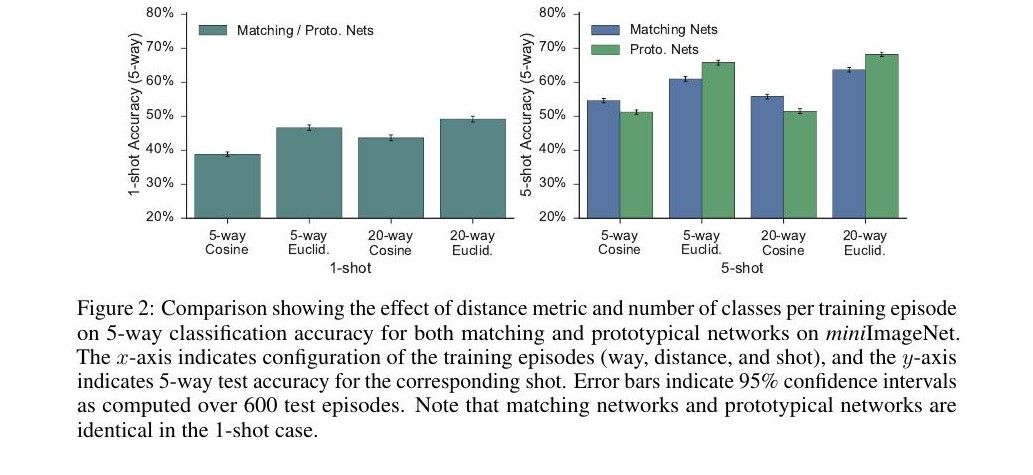
Figure 2: Comparison showing the effect of distance metric and number of classes per training episode on 5-way classification accuracy for both matching and prototypical networks on miniImageNet. The $x$-axis indicates configuration of the training episodes (way, distance, and shot), and the $y$-axis indicates 5-way test accuracy for the corresponding shot. Error bars indicate 95% confidence intervals as computed over 600 test episodes. Note that matching networks and prototypical networks are identical in the 1-shot case.

图 2：在 miniImageNet 上，距离度量以及每个训练回合的类别数，对匹配网络和原型网络 5 路分类准确率的影响。横轴表示训练回合的配置（way、距离和 shot），纵轴表示对应 shot 下的 5 路测试准确率。误差条为在 600 个测试回合上计算的 95% 置信区间。注意在 1-shot 情形下，匹配网络与原型网络是相同的。

3.3 CUB Zero-shot Classification

3.3 CUB 零样本分类

In order to assess the suitability of our approach for zero-shot learning, we also run experiments on the Caltech-UCSD Birds (CUB) 200-2011 dataset [31]. The CUB dataset contains 11,788 images of 200 bird species. We closely follow the procedure of Reed et al. [23] in preparing the data. We use their splits to divide the classes into 100 training, 50 validation, and 50 test. For images we use 1,024-dimensional features extracted by applying GoogLeNet [28] to middle, upper left, upper right, lower left, and lower right crops of the original and horizontally-flipped image[^1]. At test time we use only the middle crop of the original image. For class meta-data we use the 312-dimensional continuous attribute vectors provided with the CUB dataset. These attributes encode various characteristics of the bird species such as their color, shape, and feather patterns.

为评估该方法是否适合零样本学习，我们还在 Caltech-UCSD Birds（CUB）200-2011 数据集 [31] 上做了实验。CUB 包含 200 种鸟类的 11,788 张图像。我们基本沿用 Reed 等 [23] 的数据准备流程，按其划分把类别分成 100 个训练、50 个验证和 50 个测试。图像方面，我们对原图及其水平翻转的中心、左上、右上、左下、右下裁剪应用 GoogLeNet [28]，提取 1,024 维特征。[^1] 测试时只用原图的中心裁剪。类元数据使用 CUB 数据集提供的 312 维连续属性向量。这些属性编码鸟类的颜色、形状和羽毛图案等特征。

We learned a simple linear mapping on top of both the 1024-dimensional image features and the 312-dimensional attribute vectors to produce a 1,024-dimensional output space. For this dataset we found it helpful to normalize the class prototypes (embedded attribute vectors) to be of unit length, since the attribute vectors come from a different domain than the images. Training episodes were constructed with 50 classes and 10 query images per class. The embeddings were optimized via SGD with Adam at a fixed learning rate of $10^{-4}$ and weight decay of $10^{-5}$. Early stopping on validation loss was used to determine the optimal number of epochs for retraining on the training plus validation set.

我们在 1024 维图像特征和 312 维属性向量之上各学习一个简单的线性映射，得到 1,024 维输出空间。对这个数据集，我们发现把类原型（嵌入后的属性向量）归一化为单位长度是有帮助的，因为属性向量与图像来自不同域。训练回合由 50 个类、每类 10 张查询图像构成。嵌入用带 Adam 的 SGD 优化，学习率固定为 $10^{-4}$，权重衰减为 $10^{-5}$。用验证损失早停来确定在训练集加验证集上重新训练的最优周期数。

Model	Image Features	Image	Features	50-way Acc. 0-shot	50-way Acc.	0-shot
Image
Features
50-way Acc.
0-shot
ALE [1]	Fisher	26.9%
SJE [2]	AlexNet	40.3%
Sample Clustering [17]	AlexNet	44.3%
SJE [2]	GoogLeNet	50.1%
DS-SJE [23]	GoogLeNet	50.4%
DA-SJE [23]	GoogLeNet	50.9%
Proto. Nets (Ours)	GoogLeNet	54.6%

Image
Features

50-way Acc.
0-shot

Table 3: Zero-shot classification accuracies on CUB-200.

Model	Image Features	50-way Acc. 0-shot
ALE [1]	Fisher	26.9%
SJE [2]	AlexNet	40.3%
Sample Clustering [17]	AlexNet	44.3%
SJE [2]	GoogLeNet	50.1%
DS-SJE [23]	GoogLeNet	50.4%
DA-SJE [23]	GoogLeNet	50.9%
Proto. Nets (Ours)	GoogLeNet	54.6%

表 3：CUB-200 上的零样本分类准确率。

Table 3 shows that we achieve state-of-the-art results by a large margin when compared to methods utilizing attributes as class meta-data. We compare our method to other embedding approaches, such as ALE [1], SJE [2], and DS-SJE/DA-SJE [23]. We also compare to a recent clustering approach [17] which trains an SVM on a learned feature space obtained by fine-tuning AlexNet [14]. These zero-shot classification results demonstrate that our approach is general enough to be applied even when the data points (images) are from a different domain relative to the classes (attributes).

表 3 表明，与利用属性作为类元数据的方法相比，我们以较大优势取得了当时最好的结果。比较对象包括 ALE [1]、SJE [2] 以及 DS-SJE/DA-SJE [23] 等嵌入方法。我们也与一种近期的聚类方法 [17] 比较，后者在微调 AlexNet [14] 得到的特征空间上训练 SVM。这些零样本分类结果表明，即使数据点（图像）与类别（属性）来自不同域，我们的方法仍然足够通用。

4 Related Work

4 相关工作

The literature on metric learning is vast [15, 5]; we summarize here the work most relevant to our proposed method. Neighborhood Components Analysis (NCA) [8] learns a Mahalanobis distance to maximize K-nearest-neighbor’s (KNN) leave-one-out accuracy in the transformed space. Salakhutdinov and Hinton [27] extend NCA by using a neural network to perform the transformation. Large margin nearest neighbor (LMNN) classification [30] also attempts to optimize KNN accuracy but does so using a hinge loss that encourages the local neighborhood of a point to contain other points with the same label. The DNet-KNN [21] is another margin-based method that improves upon LMNN by utilizing a neural network to perform the embedding instead of a simple linear transformation. Of these, our method is most similar to the non-linear extension of NCA [27] because we use a neural network to perform the embedding and we optimize a softmax based on Euclidean distances in the transformed space, as opposed to a margin loss. A key distinction between our approach and non-linear NCA is that we form a softmax directly over classes, rather than individual points, computed from distances to each class’s prototype representation. This allows each class to have a concise representation independent of the number of data points and obviates the need to store the entire support set to make predictions.

度量学习的文献非常丰富 [15, 5]；这里只概述与我们方法最相关的工作。邻域成分分析（NCA）[8] 学习一种马氏距离，以最大化变换空间中 K 近邻（KNN）的留一准确率。Salakhutdinov 与 Hinton [27] 用神经网络来完成这一变换，从而扩展了 NCA。大间隔最近邻（LMNN）分类 [30] 同样试图优化 KNN 准确率，但使用合页损失，鼓励一个点的局部邻域包含其他同类点。DNet-KNN [21] 是另一种基于间隔的方法，它用神经网络而不是简单线性变换来做嵌入，从而改进了 LMNN。在这些方法中，我们的方法最接近非线性扩展的 NCA [27]，因为我们也用神经网络做嵌入，并基于变换空间中的欧氏距离优化 softmax，而不是间隔损失。我们的方法与非线性 NCA 的一个关键区别是：softmax 直接定义在类上，而不是各个点上，距离则量到每个类的原型表示。这样每个类都有一个与样本数无关的简洁表示，也就不必存储整个支持集才能做预测。

Our approach is also similar to the nearest class mean approach [19], where each class is represented by the mean of its examples. This approach was developed to rapidly incorporate new classes into a classifier without retraining, however it relies on a linear embedding and was designed to handle the case where the novel classes come with a large number of examples. In contrast, our approach utilizes neural networks to non-linearly embed points and we couple this with episodic training in order to handle the few-shot scenario. Mensink et al. attempt to extend their approach to also perform non-linear classification, but they do so by allowing classes to have multiple prototypes. They find these prototypes in a pre-processing step by using $k$-means on the input space and then perform a multi-modal variant of their linear embedding. Prototypical networks, on the other hand, learn a non-linear embedding in an end-to-end manner with no such pre-processing, producing a non-linear classifier that still only requires one prototype per class. In addition, our approach naturally generalizes to other distance functions, particularly Bregman divergences.

我们的方法也类似于最近类均值方法 [19]，后者用一类样本的均值来表示该类。这一方法是为了在不重新训练的情况下迅速把新类纳入分类器，但它依赖线性嵌入，并且面向新类带有大量样本的情形。相比之下，我们用神经网络对点做非线性嵌入，并与回合训练相结合，以应对小样本设定。Mensink 等人也曾尝试把该方法扩展到非线性分类，做法是允许每个类有多个原型。他们先在输入空间用 $k$-means 找到这些原型，再做一种多模态的线性嵌入。原型网络则端到端地学习非线性嵌入，无需这类预处理，得到的非线性分类器每类仍然只需一个原型。此外，我们的方法可以自然推广到其他距离函数，尤其是 Bregman 散度。

Another relevant few-shot learning method is the meta-learning approach proposed in Ravi and Larochelle [22]. The key insight here is that LSTM dynamics and gradient descent can be written in effectively the same way. An LSTM can then be trained to itself train a model from a given episode, with the performance goal of generalizing well on the query points. Matching networks and prototypical networks can also be seen as forms of meta-learning, in the sense that they produce simple classifiers dynamically from new training episodes; however the core embeddings they rely on are fixed after training. The FCE extension to matching nets involves a secondary embedding that depends on the support set. However, in the few-shot scenario the amount of data is so small that a simple inductive bias seems to work well, without the need to learn a custom embedding for each episode.

另一个相关的小样本学习方法是 Ravi 与 Larochelle [22] 提出的元学习路径。其关键洞见是：LSTM 的动态与梯度下降几乎可以写成同一种形式。于是可以训练一个 LSTM，让它自己从给定回合中训练一个模型，目标是在查询点上泛化良好。匹配网络和原型网络也可以看成某种形式的元学习，因为它们会根据新的训练回合动态产生简单分类器；不过它们所依赖的核心嵌入在训练之后是固定的。匹配网络的 FCE 扩展包含一个依赖于支持集的第二层嵌入。然而在小样本设定下数据极少，简单的归纳偏置似乎就已够用，不必为每个回合学习定制嵌入。

Prototypical networks are also related to the neural statistician [6] from the generative modeling literature, which extends the variational autoencoder [12, 24] to learn generative models of datasets rather than individual points. One component of the neural statistician is the “statistic network” which summarizes a set of data points into a statistic vector. It does this by encoding each point within a dataset, taking a sample mean, and applying a post-processing network to obtain an approximate posterior over the statistic vector. Edwards and Storkey test their model for one-shot classification on the Omniglot dataset by considering each character to be a separate dataset and making predictions based on the class whose approximate posterior over the statistic vector has minimal KL-divergence from the posterior inferred by the test point. Like the neural statistician, we also produce a summary statistic for each class. However, ours is a discriminative model, as befits our discriminative task of few-shot classification.

原型网络也与生成建模文献中的 neural statistician [6] 有关，后者把变分自编码器 [12, 24] 扩展为学习数据集而不是单个点的生成模型。neural statistician 的一个组件是“统计网络”，它把一组数据点汇总成统计向量：先对数据集中的每个点编码，再取样本均值，并经过后处理网络得到该统计向量的近似后验。Edwards 与 Storkey 在 Omniglot 上测试了该模型的单样本分类：把每个字符看成一个单独数据集，并基于哪一类对统计向量的近似后验与测试点推断出的后验之间 KL 散度最小来做预测。与 neural statistician 一样，我们也为每个类产生一个汇总统计量。不过我们的模型是判别式的，这与小样本分类这一判别任务相符。

With respect to zero-shot learning, the use of embedded meta-data in prototypical networks resembles the method of [3] in that both predict the weights of a linear classifier. The DS-SJE and DA-SJE approach of [23] also learns deep multimodal embedding functions for images and class meta-data. Unlike ours, they learn using an empirical risk loss. Neither [3] nor [23] uses episodic training, which allows us to help speed up training and regularize the model.

就零样本学习而言，原型网络中嵌入元数据的用法类似于 [3] 的方法，两者都预测线性分类器的权重。[23] 的 DS-SJE 和 DA-SJE 也为图像和类元数据学习深度多模态嵌入函数。与我们不同，他们使用经验风险损失。[3] 和 [23] 都没有使用回合训练；回合训练帮助我们加快训练并正则化模型。

5 Conclusion

5 结论

We have proposed a simple method called prototypical networks for few-shot learning based on the idea that we can represent each class by the mean of its examples in a representation space learned by a neural network. We train these networks to specifically perform well in the few-shot setting by using episodic training. The approach is far simpler and more efficient than recent meta-learning approaches, and produces state-of-the-art results even without sophisticated extensions developed for matching networks (although these can be applied to prototypical nets as well). We show how performance can be greatly improved by carefully considering the chosen distance metric, and by modifying the episodic learning procedure. We further demonstrate how to generalize prototypical networks to the zero-shot setting, and achieve state-of-the-art results on the CUB-200 dataset. A natural direction for future work is to utilize Bregman divergences other than squared Euclidean distance, corresponding to class-conditional distributions beyond spherical Gaussians. We conducted preliminary explorations of this, including learning a variance per dimension for each class. This did not lead to any empirical gains, suggesting that the embedding network has enough flexibility on its own without requiring additional fitted parameters per class. Overall, the simplicity and effectiveness of prototypical networks makes it a promising approach for few-shot learning.

我们提出了一种名为原型网络的简单小样本学习方法，其想法是：在神经网络学得的表示空间中，用一类样本的均值来表示该类。我们通过回合训练，专门让这些网络在小样本设定下表现良好。该方法远比近期的元学习路径更简单、也更高效，即使不采用为匹配网络开发的复杂扩展（这些扩展同样可以用于原型网络），也能得到当时最好的结果。我们说明，仔细选择距离度量并调整回合学习流程，就能大幅提升性能。我们还展示了如何把原型网络推广到零样本设定，并在 CUB-200 上取得当时最好的结果。一个自然的后续方向是使用平方欧氏距离以外的 Bregman 散度，以对应球形高斯之外的类条件分布。我们对此做了初步探索，包括为每个类的每个维度学习方差。这并没有带来经验上的收益，说明嵌入网络本身已经足够灵活，不必再为每个类拟合额外参数。总体而言，原型网络的简单与有效，使它成为小样本学习中一条有前景的路径。

Acknowledgements

We would like to thank Marc Law, Sachin Ravi, Hugo Larochelle, Renjie Liao, and Oriol Vinyals for helpful discussions. This work was supported by the Samsung GRP project and the Canadian Institute for Advanced Research.

致谢

我们感谢 Marc Law、Sachin Ravi、Hugo Larochelle、Renjie Liao 和 Oriol Vinyals 的有益讨论。本工作得到三星 GRP 项目以及加拿大高级研究院的支持。

References

参考文献

[1] Zeynep Akata, Florent Perronnin, Zaid Harchaoui, and Cordelia Schmid. Label-embedding for attribute-based classification. In Computer Vision and Pattern Recognition , pages 819–826, 2013.

[2] Zeynep Akata, Scott Reed, Daniel Walter, Honglak Lee, and Bernt Schiele. Evaluation of output embeddings for fine-grained image classification. In Computer Vision and Pattern Recognition , pages 2927–2936, 2015.

[3] Jimmy Ba, Kevin Swersky, Sanja Fidler, and Ruslan Salakhutdinov. Predicting deep zero-shot convolutional neural networks using textual descriptions. In International Conference on Computer Vision , pages 4247–4255, 2015.

[4] Arindam Banerjee, Srujana Merugu, Inderjit S Dhillon, and Joydeep Ghosh. Clustering with bregman divergences. Journal of machine learning research , 6(Oct):1705–1749, 2005.

[5] Aurélien Bellet, Amaury Habrard, and Marc Sebban. A survey on metric learning for feature vectors and structured data. arXiv preprint arXiv:1306.6709 , 2013.

[6] Harrison Edwards and Amos Storkey. Towards a neural statistician. International Conference on Learning Representations , 2017.

[7] Mohamed Elhoseiny, Babak Saleh, and Ahmed Elgammal. Write a classifier: Zero-shot learning using purely textual descriptions. In International Conference on Computer Vision , pages 2584–2591, 2013.

[8] Jacob Goldberger, Geoffrey E. Hinton, Sam T. Roweis, and Ruslan Salakhutdinov. Neighbourhood components analysis. In Advances in Neural Information Processing Systems , pages 513–520, 2004.

[9] Sepp Hochreiter and Jürgen Schmidhuber. Long short-term memory. Neural Computation , 9(8):1735–1780, 1997.

[10] Sergey Ioffe and Christian Szegedy. Batch normalization: Accelerating deep network training by reducing internal covariate shift. arXiv preprint arXiv:1502.03167 , 2015.

[11] Diederik Kingma and Jimmy Ba. Adam: A method for stochastic optimization. arXiv preprint arXiv:1412.6980 , 2014.

[12] Diederik P. Kingma and Max Welling. Auto-encoding variational bayes. arXiv preprint arXiv:1312.6114 , 2013.

[13] Gregory Koch. Siamese neural networks for one-shot image recognition. Master’s thesis, University of Toronto, 2015.

[14] Alex Krizhevsky, Ilya Sutskever, and Geoffrey E Hinton. Imagenet classification with deep convolutional neural networks. In Advances in Neural Information Processing Systems , pages 1097–1105, 2012.

[15] Brian Kulis. Metric learning: A survey. Foundations and Trends in Machine Learning , 5(4):287–364, 2012.

[16] Brenden M. Lake, Ruslan Salakhutdinov, Jason Gross, and Joshua B. Tenenbaum. One shot learning of simple visual concepts. In CogSci , 2011.

[17] Renjie Liao, Alexander Schwing, Richard Zemel, and Raquel Urtasun. Learning deep parsimonious representations. Advances in Neural Information Processing Systems , 2016.

[18] Laurens van der Maaten and Geoffrey Hinton. Visualizing data using t-sne. Journal of Machine Learning Research , 9(Nov):2579–2605, 2008.

[19] Thomas Mensink, Jakob Verbeek, Florent Perronnin, and Gabriela Csurka. Distance-based image classification: Generalizing to new classes at near-zero cost. IEEE Transactions on Pattern Analysis and Machine Intelligence , 35(11):2624–2637, 2013.

[20] Erik G Miller, Nicholas E Matsakis, and Paul A Viola. Learning from one example through shared densities on transforms. In CVPR , volume 1, pages 464–471, 2000.

[21] Renqiang Min, David A Stanley, Zineng Yuan, Anthony Bonner, and Zhaolei Zhang. A deep non-linear feature mapping for large-margin knn classification. In IEEE International Conference on Data Mining , pages 357–366, 2009.

[22] Sachin Ravi and Hugo Larochelle. Optimization as a model for few-shot learning. International Conference on Learning Representations , 2017.

[23] Scott Reed, Zeynep Akata, Bernt Schiele, and Honglak Lee. Learning deep representations of fine-grained visual descriptions. arXiv preprint arXiv:1605.05395 , 2016.

[24] Danilo Jimenez Rezende, Shakir Mohamed, and Daan Wierstra. Stochastic backpropagation and approximate inference in deep generative models. arXiv preprint arXiv:1401.4082 , 2014.

[25] Oren Rippel, Manohar Paluri, Piotr Dollar, and Lubomir Bourdev. Metric learning with adaptive density discrimination. International Conference on Learning Representations , 2016.

[26] Olga Russakovsky, Jia Deng, Hao Su, Jonathan Krause, Sanjeev Satheesh, Sean Ma, Zhiheng Huang, Andrej Karpathy, Aditya Khosla, Michael Bernstein, Alexander C. Berg, and Li Fei-Fei. Imagenet large scale visual recognition challenge. International Journal of Computer Vision , 115(3):211–252, 2015.

[27] Ruslan Salakhutdinov and Geoffrey E. Hinton. Learning a nonlinear embedding by preserving class neighbourhood structure. In AISTATS , pages 412–419, 2007.

[28] Christian Szegedy, Wei Liu, Yangqing Jia, Pierre Sermanet, Scott Reed, Dragomir Anguelov, Dumitru Erhan, Vincent Vanhoucke, and Andrew Rabinovich. Going deeper with convolutions. In Proceedings of the IEEE Conference on Computer Vision and Pattern Recognition , pages 1–9, 2015.

[29] Oriol Vinyals, Charles Blundell, Tim Lillicrap, Daan Wierstra, et al. Matching networks for one shot learning. In Advances in Neural Information Processing Systems , pages 3630–3638, 2016.

[30] Kilian Q Weinberger, John Blitzer, and Lawrence K Saul. Distance metric learning for large margin nearest neighbor classification. In Advances in Neural Information Processing Systems , pages 1473–1480, 2005.

[31] P. Welinder, S. Branson, T. Mita, C. Wah, F. Schroff, S. Belongie, and P. Perona. Caltech-UCSD Birds 200. Technical Report CNS-TR-2010-001, California Institute of Technology, 2010.

Appendix A Additional Omniglot Results

附录 A 额外的 Omniglot 结果

In Table 4 we show test classification accuracy for prototypical networks using Euclidean distance trained with 5, 20, and 60 classes per episode.

表 4 给出了使用欧氏距离、并分别以每回合 5、20 和 60 个类训练的原型网络在测试时的分类准确率。

		Train Episodes	5-way Acc.	20-way Acc.
Model	Dist.	Shot	Query	Way	1-shot	5-shot	1-shot	5-shot
Protonets	Euclid.	1	15	5	97.4%	99.3%	92.0%	97.8%
Protonets	Euclid.	1	15	20	98.7%	99.6%	95.4%	98.8%
Protonets	Euclid.	1	5	60	98.8%	99.7%	96.0%	99.0%
Protonets	Euclid.	5	15	5	96.9%	99.3%	90.7%	97.8%
Protonets	Euclid.	5	15	20	98.1%	99.6%	94.1%	98.7%
Protonets	Euclid.	5	5	60	98.5%	99.7%	94.7%	98.9%

Table 4: Additional classification accuracy results for prototypical networks on Omniglot. Configuration of training episodes is indicated by number of classes per episode (“way”), number of support points per class (“shot”) and number of query points per class (“query”). Classification accuracy was averaged over 1,000 randomly generated episodes from the test set.

		Train Episodes	5-way Acc.	20-way Acc.
Model	Dist.	Shot	Query	Way	1-shot	5-shot	1-shot	5-shot
Protonets	Euclid.	1	15	5	97.4%	99.3%	92.0%	97.8%
Protonets	Euclid.	1	15	20	98.7%	99.6%	95.4%	98.8%
Protonets	Euclid.	1	5	60	98.8%	99.7%	96.0%	99.0%
Protonets	Euclid.	5	15	5	96.9%	99.3%	90.7%	97.8%
Protonets	Euclid.	5	15	20	98.1%	99.6%	94.1%	98.7%
Protonets	Euclid.	5	5	60	98.5%	99.7%	94.7%	98.9%

表 4：原型网络在 Omniglot 上的额外分类准确率。训练回合的配置由每回合类别数（“way”）、每类支持点数（“shot”）和每类查询点数（“query”）给出。分类准确率在测试集上随机生成的 1,000 个回合上平均。

Figure 3 shows a sample t-SNE visualization [18] of the embeddings learned by prototypical networks. We visualize a subset of test characters from the same alphabet in order to gain better insight, despite the fact that classes in actual test episodes are likely to come from different alphabets. Even though the visualized characters are minor variations of each other, the network is able to cluster the hand-drawn characters closely around the class prototypes.

图 3 给出了原型网络所学嵌入的一份 t-SNE 可视化示例 [18]。为了看得更清楚，我们可视化同一字母表中的一部分测试字符，尽管实际测试回合中的类别很可能来自不同字母表。即便这些被可视化的字符彼此只是细微变体，网络仍能把手写字符紧密聚集在类原型周围。

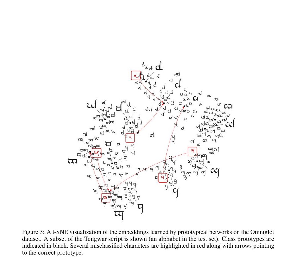
Figure 3: A t-SNE visualization of the embeddings learned by prototypical networks on the Omniglot dataset. A subset of the Tengwar script is shown (an alphabet in the test set). Class prototypes are indicated in black. Several misclassified characters are highlighted in red along with arrows pointing to the correct prototype.

图 3：原型网络在 Omniglot 数据集上学得嵌入的 t-SNE 可视化。图中展示的是 Tengwar 文字的一个子集（该字母表属于测试集）。类原型用黑色标出。若干被分错的字符用红色标出，并用箭头指向正确的原型。

Appendix B Additional miniImageNet Results

附录 B 额外的 miniImageNet 结果

In Table 5 we show the full results for the comparison of training episode configuration in Figure 2 of the main paper.

表 5 给出了正文图 2 中训练回合配置比较的完整结果。

We also compared Euclidean-distance prototypical networks trained with a different number of classes per episode. Here we vary the classes per training episode from 5 up to 30 while keeping the number of query points per class fixed at 15. The results are shown in Figure 4. Our findings indicate that construction of training episodes is an important consideration in order to achieve good results for few-shot classification. Table 6 contains the full results for this set of experiments.

我们还比较了用欧氏距离训练、但每个回合类别数不同的原型网络。这里把每个训练回合的类别数从 5 变到 30，同时把每类查询点数固定为 15。结果见图 4。我们的发现表明，训练回合的构造是获得良好小样本分类结果的重要考虑。表 6 给出了这组实验的完整结果。

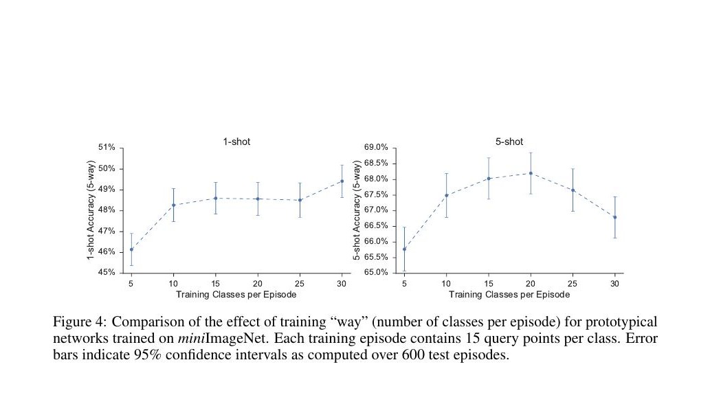
Figure 4: Comparison of the effect of training “way” (number of classes per episode) for prototypical networks trained on miniImageNet. Each training episode contains 15 query points per class. Error bars indicate 95% confidence intervals as computed over 600 test episodes.

图 4：训练 “way”（每回合类别数）对在 miniImageNet 上训练的原型网络的影响。每个训练回合每类包含 15 个查询点。误差条为在 600 个测试回合上计算的 95% 置信区间。

		Train Episodes	5-way Acc.
Model	Dist.	Shot	Query	Way	1-shot	5-shot
Matching Nets / Protonets	Cosine	1	15	5	38.82 $\pm$ 0.69%	44.54 $\pm$ 0.56%
Matching Nets / Protonets	Euclid.	1	15	5	46.61 $\pm$ 0.78%	59.84 $\pm$ 0.64%
Matching Nets / Protonets	Cosine	1	15	20	43.63 $\pm$ 0.76%	51.34 $\pm$ 0.64%
Matching Nets / Protonets	Euclid.	1	15	20	49.17 $\pm$ 0.83%	62.66 $\pm$ 0.71%
Matching Nets	Cosine	5	15	5	46.43 $\pm$ 0.74%	54.60 $\pm$ 0.62%
Matching Nets	Euclid.	5	15	5	46.43 $\pm$ 0.78%	60.97 $\pm$ 0.67%
Matching Nets	Cosine	5	15	20	46.46 $\pm$ 0.79%	55.77 $\pm$ 0.69%
Matching Nets	Euclid.	5	15	20	47.99 $\pm$ 0.79%	63.66 $\pm$ 0.68%
Protonets	Cosine	5	15	5	42.48 $\pm$ 0.74%	51.23 $\pm$ 0.63%
Protonets	Euclid.	5	15	5	44.53 $\pm$ 0.76%	65.77 $\pm$ 0.70%
Protonets	Cosine	5	15	20	42.45 $\pm$ 0.73%	51.48 $\pm$ 0.70%
Protonets	Euclid.	5	15	20	43.57 $\pm$ 0.82%	68.20 $\pm$ 0.66%

Table 5: Comparison of matching and prototypical networks on miniImageNet under cosine vs. Euclidean distance, 5-way vs. 20-way, and 1-shot vs. 5-shot. All experiments use a shared encoder for both support and query points with embedding dimension 1,600 (architecture and training details are provided in Section 3.2 of the main paper). Classification accuracy is averaged over 600 randomly generated episodes from the test set and 95% confidence intervals are shown.

		Train Episodes	5-way Acc.
Model	Dist.	Shot	Query	Way	1-shot	5-shot
Matching Nets / Protonets	Cosine	1	15	5	38.82 $\pm$ 0.69%	44.54 $\pm$ 0.56%
Matching Nets / Protonets	Euclid.	1	15	5	46.61 $\pm$ 0.78%	59.84 $\pm$ 0.64%
Matching Nets / Protonets	Cosine	1	15	20	43.63 $\pm$ 0.76%	51.34 $\pm$ 0.64%
Matching Nets / Protonets	Euclid.	1	15	20	49.17 $\pm$ 0.83%	62.66 $\pm$ 0.71%
Matching Nets	Cosine	5	15	5	46.43 $\pm$ 0.74%	54.60 $\pm$ 0.62%
Matching Nets	Euclid.	5	15	5	46.43 $\pm$ 0.78%	60.97 $\pm$ 0.67%
Matching Nets	Cosine	5	15	20	46.46 $\pm$ 0.79%	55.77 $\pm$ 0.69%
Matching Nets	Euclid.	5	15	20	47.99 $\pm$ 0.79%	63.66 $\pm$ 0.68%
Protonets	Cosine	5	15	5	42.48 $\pm$ 0.74%	51.23 $\pm$ 0.63%
Protonets	Euclid.	5	15	5	44.53 $\pm$ 0.76%	65.77 $\pm$ 0.70%
Protonets	Cosine	5	15	20	42.45 $\pm$ 0.73%	51.48 $\pm$ 0.70%
Protonets	Euclid.	5	15	20	43.57 $\pm$ 0.82%	68.20 $\pm$ 0.66%

表 5：在 miniImageNet 上比较匹配网络与原型网络：余弦距离对欧氏距离、5-way 对 20-way、以及 1-shot 对 5-shot。所有实验对支持和查询点使用共享编码器，嵌入维度为 1,600（架构与训练细节见正文 3.2 节）。分类准确率在测试集上随机生成的 600 个回合上平均，并给出 95% 置信区间。

		Train Episodes	5-way Acc.
Model	Dist.	Shot	Query	Way	1-shot	5-shot
Protonets	Euclid.	1	15	5	46.14 $\pm$ 0.77%	61.36 $\pm$ 0.68%
Protonets	Euclid.	1	15	10	48.27 $\pm$ 0.79%	64.18 $\pm$ 0.68%
Protonets	Euclid.	1	15	15	48.60 $\pm$ 0.76%	64.62 $\pm$ 0.66%
Protonets	Euclid.	1	15	20	48.57 $\pm$ 0.79%	65.04 $\pm$ 0.69%
Protonets	Euclid.	1	15	25	48.51 $\pm$ 0.83%	64.63 $\pm$ 0.69%
Protonets	Euclid.	1	15	30	49.42 $\pm$ 0.78%	65.38 $\pm$ 0.68%
Protonets	Euclid.	5	15	5	44.53 $\pm$ 0.76%	65.77 $\pm$ 0.70%
Protonets	Euclid.	5	15	10	45.09 $\pm$ 0.79%	67.49 $\pm$ 0.70%
Protonets	Euclid.	5	15	15	44.07 $\pm$ 0.80%	68.03 $\pm$ 0.66%
Protonets	Euclid.	5	15	20	43.57 $\pm$ 0.82%	68.20 $\pm$ 0.66%
Protonets	Euclid.	5	15	25	43.32 $\pm$ 0.79%	67.66 $\pm$ 0.68%
Protonets	Euclid.	5	15	30	41.38 $\pm$ 0.81%	66.79 $\pm$ 0.66%

Table 6: Effect of training “way” (number of classes per training episode) for prototypical networks with Euclidean distance on miniImageNet. The number of query points per class in training episodes was fixed at 15. Classification accuracy is averaged over 600 randomly generated episodes from the test set and 95% confidence intervals are shown.

		Train Episodes	5-way Acc.
Model	Dist.	Shot	Query	Way	1-shot	5-shot
Protonets	Euclid.	1	15	5	46.14 $\pm$ 0.77%	61.36 $\pm$ 0.68%
Protonets	Euclid.	1	15	10	48.27 $\pm$ 0.79%	64.18 $\pm$ 0.68%
Protonets	Euclid.	1	15	15	48.60 $\pm$ 0.76%	64.62 $\pm$ 0.66%
Protonets	Euclid.	1	15	20	48.57 $\pm$ 0.79%	65.04 $\pm$ 0.69%
Protonets	Euclid.	1	15	25	48.51 $\pm$ 0.83%	64.63 $\pm$ 0.69%
Protonets	Euclid.	1	15	30	49.42 $\pm$ 0.78%	65.38 $\pm$ 0.68%
Protonets	Euclid.	5	15	5	44.53 $\pm$ 0.76%	65.77 $\pm$ 0.70%
Protonets	Euclid.	5	15	10	45.09 $\pm$ 0.79%	67.49 $\pm$ 0.70%
Protonets	Euclid.	5	15	15	44.07 $\pm$ 0.80%	68.03 $\pm$ 0.66%
Protonets	Euclid.	5	15	20	43.57 $\pm$ 0.82%	68.20 $\pm$ 0.66%
Protonets	Euclid.	5	15	25	43.32 $\pm$ 0.79%	67.66 $\pm$ 0.68%
Protonets	Euclid.	5	15	30	41.38 $\pm$ 0.81%	66.79 $\pm$ 0.66%

表 6：训练 “way”（每个训练回合的类别数）对使用欧氏距离的原型网络在 miniImageNet 上的影响。训练回合中每类查询点数固定为 15。分类准确率在测试集上随机生成的 600 个回合上平均，并给出 95% 置信区间。