The Polar Express: Optimal Matrix Sign Methods and Their Application to the Muon Algorithm
The Polar Express: Optimal Matrix Sign Methods and Their Application to the Muon Algorithm
Polar Express:最优矩阵符号方法及其在 Muon 算法中的应用
Noah Amsel Thanks: New York University. noah.amsel@nyu.edu David Persson Thanks: New York University and Flatiron Institute. dup210@nyu.edu , dpersson@flatironinstitute.org Christopher Musco Thanks: New York University. cmusco@nyu.edu Robert M. Gower Thanks: Flatiron Institute. rgower@flatironinstitute.org
Abstract
摘要
Computing the polar decomposition and the related matrix sign function has been a well-studied problem in numerical analysis for decades. Recently, it has emerged as an important subroutine within the Muon algorithm for training deep neural networks. However, the requirements of this application differ sharply from classical settings: deep learning demands GPU-friendly algorithms that prioritize high throughput over high precision. We introduce Polar Express, a new method for computing the polar decomposition. Like Newton–Schulz and other classical polynomial methods, our approach uses only matrix-matrix multiplications, making it very efficient on GPUs. Inspired by earlier work of Chen & Chow and Nakatsukasa & Freund, Polar Express adapts the update rule at each iteration by solving a minimax optimization problem. We prove that this strategy minimizes error in a worst-case sense, allowing Polar Express to converge as rapidly as possible both in the early iterations and asymptotically. We also address finite-precision issues, making it practical to use in bfloat16. When integrated into the Muon training framework, our method leads to consistent improvements in validation loss when training a GPT-2 model on one billion tokens from the FineWeb dataset, outperforming recent alternatives across a range of learning rates.
计算极分解以及与之相关的矩阵符号函数,是数值分析里研究了数十年的老问题。最近它又成了训练深度网络的 Muon 算法里的关键子程序。不过,这一应用提出的要求与经典场景差得很远:深度学习需要照顾 GPU 的算法,更看重吞吐,而不是极高的精度。我们提出 Polar Express,一种新的极分解算法。它和 Newton–Schulz 以及其他经典多项式方法一样,只用矩阵-矩阵乘法,因而在 GPU 上很高效。受 Chen & Chow 以及 Nakatsukasa & Freund 较早工作的启发,Polar Express 在每一步都通过求解一个 minimax 优化问题来调整更新规则。我们证明这一策略能在最坏情形下把误差压到最小,从而让 Polar Express 无论在前期迭代还是在渐近阶段都能尽快收敛。我们还处理了有限精度下的问题,使其能切实用于 bfloat16。把该方法嵌进 Muon 训练框架后,在 FineWeb 数据集的 10 亿 token 上训练 GPT-2 时,验证损失得到了稳定的改善,并在一系列学习率下都优于近期的替代方法。
1 Introduction
1 引言
Contents
Advanced linear algebra is making its way into deep learning. Efficient algorithms for computing matrix functions have found exciting new applications in training neural networks. In particular, approximations to the matrix-inverse are used in the full Adagrad method [13], the matrix square-root and quarter-root appear as subroutines in the Shampoo and Soap optimizers [17, 43, 47], and most recently, the matrix sign function has become a key ingredient of the Muon optimizer [5, 4, 22].
目录
高等线性代数正在进入深度学习。计算矩阵函数的高效算法,已经在神经网络训练里找到了令人兴奋的新用途。具体来说,矩阵求逆的近似出现在完整的 Adagrad 方法中 [13],矩阵平方根和四分之一次根是 Shampoo 与 Soap 优化器的子程序 [17, 43, 47],而最近,矩阵符号函数又成了 Muon 优化器的关键构件 [5, 4, 22]。
While the problem of computing these matrix functions has been studied by numerical analysts for decades, applications in deep learning come with different requirements than those in computational science. For deep learning, it is critical to take maximum advantage of GPU-friendly operations like matrix-matrix products and to avoid less parallel operations. Moreover, memory overhead must be small to handle large models. On the other hand, high accuracy is typically less important; the gold standard of sixteen digits of accuracy is overkill in deep learning.
尽管计算这些矩阵函数的问题已被数值分析学家研究了数十年,深度学习应用提出的要求与计算科学并不相同。对深度学习来说,关键是尽量用满 GPU 友好的操作(例如矩阵-矩阵乘法),并避开并行度较差的运算。内存开销也必须很小,才能撑住大模型。另一方面,高精度通常并不那么重要;科学计算里追求的十六位有效数字,对深度学习来说过头了。
Given these considerations, there is a need to develop new matrix function methods that are tailor-made for deep learning applications. We take on this challenge by designing a state-of-the-art, GPU-friendly algorithm for computing the matrix sign function, or more generally, for computing the polar decomposition of a rectangular matrix. We apply our new Polar Express method (Algorithm 1) to compute the descent direction in the increasingly popular Muon optimizer. In Figure 1, we show that using Polar Express within Muon consistently results in lower validation loss across all learning rates when training a GPT-2 model, as compared to other matrix sign methods [9, 44, 22].
基于这些考虑,有必要专门为深度学习设计新的矩阵函数方法。我们接受这一挑战,设计了一种面向 GPU、用于计算矩阵符号函数——更一般地说,用于计算矩形矩阵极分解——的先进算法。我们把新的 Polar Express 方法(算法 1)用到日益流行的 Muon 优化器里,去计算下降方向。图 1 表明,在训练 GPT-2 时,把 Polar Express 放进 Muon,在所有学习率下都能得到更低的验证损失,优于其他矩阵符号方法 [9, 44, 22]。
from itertools import repeat
import torch
coeffs_list = [
(8.28721201814563, -23.595886519098837, 17.300387312530933),
(4.107059111542203, -2.9478499167379106, 0.5448431082926601),
(3.9486908534822946, -2.908902115962949, 0.5518191394370137),
(3.3184196573706015, -2.488488024314874, 0.51004894012372),
(2.300652019954817, -1.6689039845747493, 0.4188073119525673),
(1.891301407787398, -1.2679958271945868, 0.37680408948524835),
(1.8750014808534479, -1.2500016453999487, 0.3750001645474248),
(1.875, -1.25, 0.375), # subsequent coeffs equal this numerically
]
safety factor for numerical stability (but exclude last polynomial)
coeffs_list = [(a / 1.01, b / 1.013, c / 1.015)
for (a, b, c) in coeffs_list[:-1]] + [coeffs_list[-1]]
@torch.compile
def PolarExpress(G: torch.Tensor, steps: int) -> torch.Tensor:
assert G.ndim >= 2
X = G.bfloat16() # for speed
if G.size(-2) > G.size(-1): X = X.mT # this reduces FLOPs
X = X / (X.norm(dim=(-2, -1), keepdim=True) * 1.01)
hs = coeffs_list[:steps] + list(
repeat(coeffs_list[-1], steps - len(coeffs_list)))
for a, b, c in hs:
A = X @ X.mT
B = b * A + c * A @ A
X = a * X + B @ X # X <- aX + bX^3 + cX^5
if G.size(-2) > G.size(-1): X = X.mT
return X
Algorithm 1 Python code for the Polar Express of degree = 5.
from itertools import repeat
import torch
coeffs_list = [
(8.28721201814563, -23.595886519098837, 17.300387312530933),
(4.107059111542203, -2.9478499167379106, 0.5448431082926601),
(3.9486908534822946, -2.908902115962949, 0.5518191394370137),
(3.3184196573706015, -2.488488024314874, 0.51004894012372),
(2.300652019954817, -1.6689039845747493, 0.4188073119525673),
(1.891301407787398, -1.2679958271945868, 0.37680408948524835),
(1.8750014808534479, -1.2500016453999487, 0.3750001645474248),
(1.875, -1.25, 0.375), # subsequent coeffs equal this numerically
]
safety factor for numerical stability (but exclude last polynomial)
coeffs_list = [(a / 1.01, b / 1.013, c / 1.015)
for (a, b, c) in coeffs_list[:-1]] + [coeffs_list[-1]]
@torch.compile
def PolarExpress(G: torch.Tensor, steps: int) -> torch.Tensor:
assert G.ndim >= 2
X = G.bfloat16() # for speed
if G.size(-2) > G.size(-1): X = X.mT # this reduces FLOPs
X = X / (X.norm(dim=(-2, -1), keepdim=True) * 1.01)
hs = coeffs_list[:steps] + list(
repeat(coeffs_list[-1], steps - len(coeffs_list)))
for a, b, c in hs:
A = X @ X.mT
B = b * A + c * A @ A
X = a * X + B @ X # X <- aX + bX^3 + cX^5
if G.size(-2) > G.size(-1): X = X.mT
return X
算法 1 次数 的 Polar Express 的 Python 代码。
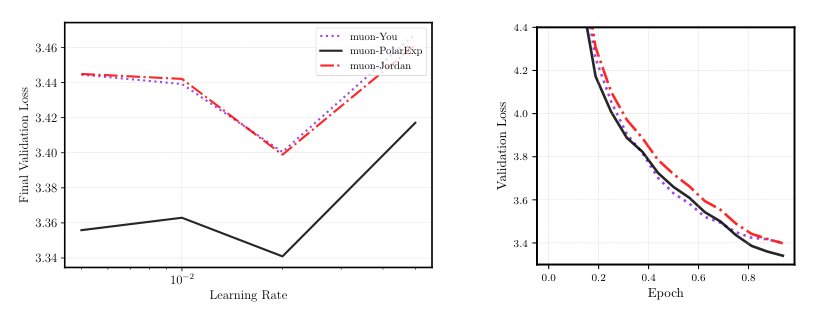
Figure 1: Training a GPT-2-Large model (774M params) on 1 billion tokens from the FineWeb dataset [2]. The label muon- refers to implementing Muon using to compute the polar factor. Left: final validation loss across learning rates. Right: validation loss across epochs using the best learning rate. The best learning rate () and final validation loss for each method was adamw : , muon-You : , muon-Jordan : and muon-PolarExp : .
图 1:在 FineWeb 数据集 [2] 的 10 亿 token 上训练 GPT-2-Large 模型(774M 参数)。标签 muon- 表示用 来计算极因子,以实现 Muon。左:各学习率下的最终验证损失。右:采用各自最优学习率时,验证损失随 epoch 的变化。各方法的最优学习率()和最终验证损失分别为:adamw :,muon-You :,muon-Jordan :,muon-PolarExp :。
1.1 The Muon Method
1.1 Muon 方法
The Muon optimizer has recently gained popularity for training large language models, often outperforming state-of-the-art adaptive gradient methods like Adam and AdamW [26, 31]. Muon has been used to set records for the NanoGPT speedrun [22] and to expand the Pareto frontier of performance versus training FLOPs for large language models [30, 42].
Muon 优化器最近在训练大语言模型时颇受欢迎,常常超过 Adam 和 AdamW 这类先进的自适应梯度方法 [26, 31]。Muon 曾用来刷新 NanoGPT speedrun 纪录 [22],也把大语言模型在性能与训练 FLOPs 之间的帕累托前沿往外推了一截 [30, 42]。
The Muon update rule [5] is defined as follows. Let be the learning rate and momentum coefficient hyperparameters. (By default, .) Let be the weight matrix of a given neural network layer at iteration , and let be its (stochastic) gradient. Let be the running momentum estimate of the gradient, where . The Muon update is given by
Muon 的更新规则 [5] 如下。设 为学习率和动量系数超参数(默认 )。设 为某层网络在第 步的权重矩阵, 为其(随机)梯度。设 为梯度的滑动动量估计,且 。Muon 更新由下式给出
Whereas standard stochastic gradient descent (SGD) with momentum updates the weight matrix by taking a step in the direction , the Muon method steps in the direction , where denotes the closest semi-orthogonal matrix to [19, Chapter 8]. Concretely, if is the singular value decomposition (SVD) of , then
标准的带动量随机梯度下降(SGD)沿 方向更新权重;Muon 则沿 迈步,其中 表示离 最近的半正交矩阵 [19, 第 8 章]。具体来说,若 是 的奇异值分解(SVD),则
The matrix can be seen as a generalization of the matrix sign function to rectangular matrices [3]. Indeed, when is square symmetric with eigendecomposition , exactly coincides with the matrix sign function [19, Chapter 5]. Equivalently, is the left orthogonal factor of the polar decomposition of [19, Chapter 8]. The motivation for Muon is that gives the steepest-descent direction with respect to the spectral norm (instead of the Frobenius norm, as in standard SGD).
矩阵 可以看成矩阵符号函数向矩形矩阵的推广 [3]。确实,当 为方阵且对称、特征分解为 时, 恰好等于矩阵符号函数 [19, 第 5 章]。等价地说, 就是 的极分解中左侧的正交因子 [19, 第 8 章]。Muon 的动机是: 给出的是关于谱范数的最速下降方向(而标准 SGD 用的是 Frobenius 范数)。
Recent work [40] shows that Muon can be viewed as a conditional gradient (Frank-Wolfe) method with a trust region defined by the spectral norm. In the same work, the authors also provide a convergence theory for the smooth and non-convex setting, as well as for the stochastic non-convex case. The analysis of Muon was further refined in [41], which proves convergence under a layerwise -smoothness assumption, in both the stochastic non-convex and stochastic Polyak–Łojasiewicz settings. We refer the reader to [22] and [5] for further background. In this paper, we take the Muon update rule as given and focus on the problem of efficiently computing the polar decomposition .
近期工作 [40] 表明,Muon 可以看成一种条件梯度(Frank-Wolfe)方法,其信赖域由谱范数划定。同一工作还给出了光滑非凸情形以及随机非凸情形下的收敛理论。[41] 进一步细化了分析,在逐层 -光滑假设下,证明了随机非凸和随机 Polyak–Łojasiewicz 两种设定中的收敛性。更多背景见 [22] 和 [5]。本文把 Muon 的更新规则当作给定,集中讨论如何高效计算极分解 。
1.2 Computing the Polar Factor
1.2 计算极因子
Although can be computed directly via an SVD in time, doing so is prohibitively expensive in deep learning applications, especially as standard SVD algorithms fail to take full advantage of the parallelism available on GPUs. There has been significant work on highly-parallel methods for the SVD, but the most common approaches actually require computing the matrix-sign function as a subroutine [33, 35]. Numerical analysts have spent decades developing iterative methods for computing . This rich line of work includes Newton–Schulz [19, Chapter 8], Padé iteration [25, 18], the Newton and scaled Newton iterations [19, Chapter 8], the QWHD iteration [32, 35], and Zolo-pd (Zolotarev polar decomposition) [33]. Unfortunately, as discussed in Section 2, most of these methods are based on rational approximations to the function and require computing matrix inverses or QR decompositions. Such methods are ill-suited to GPU acceleration and deep learning applications. In contrast, the older Newton-Schulz method is based on polynomial approximation of and uses only matrix-matrix products. Thus, Muon initially used Newton-Schulz [4]. Indeed, Muon stands for “MomentUm Orthogonalized by Newton-Schulz” [22].
虽然可以直接用 SVD 在 时间内算出 ,这在深度学习里贵得难以承受,尤其是标准 SVD 算法没法充分利用 GPU 上的并行能力。高度并行的 SVD 方法也有不少研究,但最常见的路线其实还是把计算矩阵符号函数当作子程序 [33, 35]。数值分析学家花了数十年发展计算 的迭代法。这条丰富的脉络包括 Newton–Schulz [19, 第 8 章]、Padé 迭代 [25, 18]、Newton 迭代及其缩放版本 [19, 第 8 章]、QWHD 迭代 [32, 35],以及 Zolo-pd(Zolotarev 极分解)[33]。可惜,如第 2 节所讨论的,这些方法大多基于对函数 的有理逼近,需要计算矩阵逆或 QR 分解。这类方法既不适合 GPU 加速,也不适合深度学习。相比之下,更早的 Newton-Schulz 方法基于对 的多项式逼近,只用矩阵-矩阵乘法。因此 Muon 起初采用的就是 Newton-Schulz [4]。Muon 这个名字正是 “MomentUm Orthogonalized by Newton-Schulz” 的缩写 [22]。
The Newton-Schulz methods.
Newton-Schulz constructs a sequence of approximations as follows:
Newton-Schulz 方法。
Newton-Schulz 按如下方式构造一列近似 :
At each iteration, this rule effectively applies the cubic polynomial to each singular value of . The scalar fixed-point iteration converges to as , provided . As a result, the matrix iteration satisfies . Higher-degree versions of Newton-Schulz follow the same principle. For example, the degree-5 polynomial converges even faster. The Newton-Schulz iterations converge super-exponentially when is sufficiently close to , but they suffer from slow initial convergence; when is far from , the approximation improves slowly over the first few iterations.
每一步迭代,这条规则实际上是把三次多项式 作用到 的每一个奇异值上。标量不动点迭代 在 时会收敛到 (当 )。因此矩阵迭代满足 。更高次数的 Newton-Schulz 遵循同一原理。例如五次多项式 收敛得更快。当 已经足够接近 时,Newton-Schulz 迭代超指数收敛;但起步很慢:当 离 还远时,前几步近似改善得很有限。
The Jordan and You methods.
In Muon, high accuracy approximations to are usually not necessary. The primary goal is instead to compute a coarse approximation in as few iterations as possible. To accelerate convergence in the low-accuracy regime, Jordan recently proposed a fixed-point iteration based on the polynomial [22], which was found using a heuristic numerical search. Unlike Newton-Schulz, the scheme that Jordan proposed does not converge to . Instead, it plateaus at an error of . However, it reaches this level of accuracy rapidly. As a result, when the number of iterations is smaller than about , Jordan’s method outperforms the Newton-Schulz iteration. Building on this idea, You [9] proposed a method that applies six different polynomial updates in succession, which were again found by heuristic search. This method achieves better accuracy than Jordan’s but still fails to converge.
Jordan 方法与 You 方法。
在 Muon 里,通常并不需要高精度地逼近 。首要目标是用尽量少的迭代算出一个粗糙近似。为了加快低精度区间里的收敛,Jordan 最近提出了一种基于多项式 的不动点迭代 [22],系数来自启发式数值搜索。与 Newton-Schulz 不同,Jordan 提出的格式并不会收敛到 ,而是在误差约 处停下。不过它达到这一精度的速度很快。因此当迭代次数大约小于 时,Jordan 的方法会超过 Newton-Schulz 迭代。顺着这一思路,You [9] 提出连续使用六种不同的多项式更新,同样由启发式搜索得到。该方法精度优于 Jordan,但仍然不会真正收敛。
We introduce a new method. In particular, we derive polynomial update rules that are optimal at every iteration, outperforming all previous polynomial methods in our setting.
我们提出一种新方法。具体来说,我们导出在每一步都最优的多项式更新规则,在我们所关心的设定下超过此前所有多项式方法。
1.3 Contributions
1.3 贡献
We present Polar Express, an iterative method for approximating . Our method dynamically adapts the polynomial update rule at each iteration, prioritizing rapid progress in the initial stage and high accuracy in the later stage. Polar Express constructs polynomials so that the resulting composition is the optimal approximation to the sign function with respect to the supremum () norm (Theorem 4.1). By iteratively applying these polynomials to , Polar Express computes an approximation to that is optimal in the worst-case at every iteration. Our method converges to super-exponentially (Theorem 4.3), and it quickly reaches a good approximation within just five to ten iterations. This early-stage acceleration is especially valuable in deep learning applications, where runtime efficiency takes precedence over high accuracy. In contrast, classical methods like Newton-Schulz suffer from a slow initial convergence, while recent heuristic proposals [22, 9] fail to converge. Our method is efficient to run on GPUs, using only a few matrix-matrix products per iteration.[^1]
我们提出 Polar Express,一种逼近 的迭代法。该方法会动态调整每一步的多项式更新规则,前期优先快速推进,后期再追求高精度。Polar Express 构造多项式 ,使得所得复合是关于上确界()范数对符号函数的最优逼近(定理 4.1)。把这些多项式迭代作用到 上,Polar Express 就能在每一步都得到最坏情形下最优的 近似。我们的方法超指数收敛到 (定理 4.3),并且只需五到十步就能得到不错的近似。这种前期加速对深度学习尤其有价值,因为那里更看重运行效率而不是高精度。相比之下,Newton-Schulz 这类经典方法起步很慢,而近期的启发式方案 [22, 9] 又无法真正收敛。我们的方法在 GPU 上很高效,每步只用几次矩阵-矩阵乘法。[^1]
We give an explicit instantiation of Polar Express in Algorithm 1, which incorporates minor modifications to make it compatible with half-precision arithmetic (see Section 4.4). Algorithm 1 can be used as a drop-in replacement for previous methods. In numerical experiments, Polar Express outperforms previous methods on synthetic matrices and gradient matrices from a GPT-2 transformer (Figure 4). We demonstrate the effectiveness of using Polar Express within the Muon optimizer in Figure 1, showing that it consistently improves the training of GPT-2 language models on 1 billion tokens of the FineWeb dataset [2].
我们在算法 1 中给出 Polar Express 的一个显式实例,其中加入了少许改动,使之能兼容半精度算术(见第 4.4 节)。算法 1 可以当作此前方法的即插即用替换。数值实验中,Polar Express 在合成矩阵以及来自 GPT-2 Transformer 的梯度矩阵上都超过了以往方法(图 4)。图 1 展示了把 Polar Express 放进 Muon 优化器后的效果:在 FineWeb 数据集 [2] 的 10 亿 token 上训练 GPT-2 语言模型时,它稳定地改善了训练表现。
Notation.
We let and denote the Frobenius norm and spectral norm (largest singular value) of a matrix , respectively. We denote the spectrum (set of singular values) by .
记号。
我们分别用 和 表示矩阵 的 Frobenius 范数和谱范数(最大奇异值)。用 表示谱(奇异值集合)。
Let be the set of polynomials of degree at most . For odd , denotes the set of polynomials of degree at most containing only odd-degree monomials. For a polynomial , is its degree. Let be the scalar sign function, which satisfies , if and if .
设 为次数至多为 的多项式集合。对奇数 , 表示次数至多为 、且只含奇次单项式的多项式集合。对多项式 , 为其次数。设 为标量符号函数,满足 , 时 , 时 。
For a polynomial and a matrix with rank reduced SVD given by and positive singular values , we define , where is the diagonal matrix with diagonal entries for .
对多项式 ,以及具有降秩 SVD 、正奇异值为 的矩阵 ,我们定义 ,其中 是对角元为 ()的对角矩阵。
2 Related Work
2 相关工作
Computing is an important and longstanding problem in numerical linear algebra, with applications spanning electronic structure calculations, lattice quantum chromodynamics, orthogonal Procrustes analysis, parallel algorithms for computing the SVD, and beyond; see e.g. [18, 23, 8, 16, 36, 45].
计算 是数值线性代数里一个重要而悠久的问题,应用涵盖电子结构计算、格点量子色动力学、正交 Procrustes 分析、并行 SVD 算法等等;参见 [18, 23, 8, 16, 36, 45]。
Newton-Schulz and polynomial Padé methods.
The earliest methods in the literature are polynomial iterations like (2). Several nearly simultaneous papers introduced the family of polynomial Padé iterations, comprising Newton-Schulz and its higher-degree analogues [27, 6, 18, 29]. These higher-degree methods are also sometimes called “Newton-Schulz”; when doing so, we will specify the degree for clarity. In these methods, each iteration refines the current approximation by applying a low-degree odd matrix polynomial, where any odd monomial is defined for rectangular matrices by the formula . Our Polar Express method also takes this form, though unlike Newton-Schulz, it changes the polynomial at each iteration.
Newton-Schulz 与多项式 Padé 方法。
文献中最早的方法是形如 (2) 的多项式迭代。几篇几乎同时出现的论文引入了多项式 Padé 迭代族,其中包括 Newton-Schulz 及其更高次数的同类方法 [27, 6, 18, 29]。这些更高次数的方法有时也被称作 “Newton-Schulz”;这样称呼时我们会标明次数以免混淆。在这些方法里,每一步都用一个低次奇次矩阵多项式来改进当前近似 ,其中任意奇次单项式 对矩形矩阵由公式 定义。我们的 Polar Express 也取这一形式,不过与 Newton-Schulz 不同,它在每一步都会更换多项式。
The polynomials used in Padé methods are chosen to match the value and first few derivatives of at the points . For instance, the update rule of the third method in this family is defined by , which is the unique degree-7 polynomial satisfying and . These methods converge so long as all singular values of lie in , a condition guaranteed by the initialization of (2). Furthermore, the order of convergence of the degree method is [6]. In particular, the Newton-Schulz method () converges quadratically.
Padé 方法所用的多项式,是为了在 处匹配 的函数值及其前若干阶导数。例如该族中第三种方法的更新规则由 给出,这是满足 且 的唯一七次多项式。只要 的全部奇异值落在 内——(2) 的初始化就保证了这一点——这些方法就会收敛。此外,次数为 的方法收敛阶为 [6]。特别地,Newton-Schulz 方法()二次收敛。
Newton’s method and rational Padé.
In the numerical analysis literature, polynomial methods were succeeded by rational iterations like Newton’s method [18], defined as follows[^2]:
Newton 方法与有理 Padé。
在数值分析文献中,多项式方法之后出现的是像 Newton 方法这样的有理迭代 [18],定义如下[^2]:
Newton’s method also converges quadratically. Like Newton-Schulz, it works because the rational function has a stable fixed point at ; unlike for Newton-Schulz, this point is a global attractor for the whole positive real line. At first glance, Newton’s method has nothing to do with the Padé iterations discussed above. However, after a change of variables , it can be reinterpreted as , which is sometimes called inverse Newton. Observing that satisfies and , we see that (inverse) Newton is also a Padé method, though a rational rather than polynomial one. In fact, given a odd degree for the numerator and an even degree for the denominator, there is a unique rational function that matches the value and first derivatives of at . This directly yields a Padé method for computing whose order of convergence is . For instance, is called Halley’s method, which converges cubically. When , we recover the polynomial Padé methods.
Newton 方法同样二次收敛。和 Newton-Schulz 一样,它之所以有效,是因为有理函数 在 处有一个稳定不动点;与 Newton-Schulz 不同的是,这个点是整条正实轴的全局吸引子。乍看之下,Newton 方法与上面讨论的 Padé 迭代毫无关系。不过做变量替换 之后,它可以改写成 ,有时称作逆 Newton。注意到 满足 且 ,可见(逆)Newton 其实也是一种 Padé 方法,只不过是有理的而非多项式的。事实上,给定分子的奇次数 和分母的偶次数 ,存在唯一的有理函数能在 处匹配 的函数值及其前 阶导数。这直接给出一种计算 的 Padé 方法,收敛阶为 。例如 称为 Halley 方法,三次收敛。当 时,就回到多项式 Padé 方法。
There are two main weakness of Newton’s method and the Padé iterations: slow convergence in the initial phase and the need to compute explicit inverses. To accelerate initial convergence, Higham popularized the technique of rescaling the matrix after every Newton iteration [18]. Intuitively, rescaling so that centers the spectrum around , where convergence is fastest. Several easily-computable choices of scaling factor exist to accomplish this approximately. Note that this rescaling scheme would fail for Newton-Schulz, which likewise suffers from slow initial convergence but which would diverge if .
Newton 方法与 Padé 迭代有两个主要弱点:初期收敛慢,以及需要显式求逆。为加快初期收敛,Higham 推广了每步 Newton 迭代后重新缩放矩阵的技巧 [18]。直观上,把 缩放到 ,就能把谱居中到 附近,而那里收敛最快。有若干易于计算的缩放因子可以近似做到这一点。需要注意,这种缩放方案对 Newton-Schulz 行不通:后者同样受初期收敛慢的困扰,但如果 它还会发散。
Computing matrix inverses is difficult to parallelize and to implement stably in low precision arithmetic. However, a trick was developed for stably computing many rational methods without explicit inverses; QR decompositions can be used instead [32, 49]. Applying this trick to Halley’s method and combining with a special rescaling scheme yields the QDWH (QR-based dynamically weighted Halley) method, which converges in just six iterations for any reasonably conditioned matrix [32].
计算矩阵逆既难并行,也难在低精度算术里稳定实现。不过人们找到了一个窍门,可以在不显式求逆的情况下稳定地计算许多有理方法:改用 QR 分解 [32, 49]。把这一窍门用到 Halley 方法上,再配上一种特殊的缩放方案,就得到 QDWH(基于 QR、动态加权的 Halley)方法,对任何条件数不太离谱的矩阵都能在六步内收敛 [32]。
Adaptive rational methods from optimal approximations.
A landmark 2016 paper introduced a new paradigm to design iterative methods for computing [33]. We describe this paradigm in more detail in Section 4, but the main insight is as follows. Padé methods choose the update rule to be an approximation to of a given degree that is optimally accurate in the neighborhood of . Instead, we should choose the approximation to that is optimal over an interval that contains the singular values. Moreover, after each step of the algorithm, the range of the singular values changes; therefore, we adapt the update rule at each iteration to match the new interval. When the range of the singular values is large, this approach ensures that the update rule shrinks it as quickly as possible. As the algorithm proceeds and the interval shrinks to a small neighborhood of , the update rule approaches that of a Padé method, maintaining the same high order of convergence as it has.
由最优逼近得到的自适应有理方法。
2016 年一篇标志性论文引入了一种设计 迭代法的新范式 [33]。我们在第 4 节更详细地描述这一范式,其核心洞见如下。Padé 方法把更新规则选成在 邻域内、给定次数下对 最优精确的逼近。相反,我们应当选择在包含奇异值的区间 上最优的 逼近。而且每走一步,奇异值的取值范围都会变;因此我们在每一步都按新区间调整更新规则。当奇异值范围很大时,这种方法能尽快把它缩小。随着算法推进、区间收缩到 的一个小邻域,更新规则会逼近 Padé 方法,从而保持同样高的收敛阶。
Within the class of odd rational functions whose numerators and denominators have degree and , respectively, an explicit formula for this optimal approximation to on any interval was found by Zolotarev. It was shown that these rationals have remarkable convergence properties for any [33]. For , this optimal approximation coincides exactly with the dynamically weighted Halley’s method (QDWH) referenced above. For even faster convergence than QDWH, [33] proposed the zolo-pd method, which uses . Finally, these methods all admit the same QR-based implementation trick as QDWH.
在分子、分母次数分别为 和 的奇次有理函数类中,Zolotarev 给出了任意区间 上对 最优逼近的显式公式。已经证明,这些有理函数对任意 都有出色的收敛性质 [33]。当 时,这一最优逼近恰好就是上面提到的动态加权 Halley 方法(QDWH)。为了比 QDWH 收敛得更快,[33] 提出了取 的 zolo-pd 方法。这些方法都可以沿用 QDWH 那套基于 QR 的实现技巧。
Adaptive polynomial methods.
In this paper, we adopt the paradigm of zolo-pd [33] but with polynomials rather than rationals of degree . This choice avoids the need for QR factorizations, relying solely on GPU-friendly matrix-matrix multiplications in low-precision arithmetic. While this class of methods has not been fully developed in the numerical analysis literature, similar ideas have been rediscovered in different guises. In an unpublished manuscript that predates zolo-pd, Chen and Chow [11] describe a rescaling strategy for Newton-Schulz. Though motivated differently, their method is equivalent to ours for degree-3 polynomials. They also observe numerical instability that prevents the method from converging to all the way to machine precision. Using the insights of [34], they propose a simple mitigation for this issue that we adopt in Section 4.4. Our work gives this method a theoretical foundation that connects it to the paradigm of zolo-pd, and we prove its optimality in the sense of (6). In addition, we study odd polynomials of arbitrary degree and focus particularly on the degree-5 case. Independently, a group of cryptographers developed a similar method for approximating the scalar function in the context of homomorphic encryption schemes [28]. Their focus is mainly on tuning the analogues in their setting of the polynomial degree and number of iterations, whereas we focus on demonstrating optimality and efficiently constructing the update polynomials for degree and . In addition, we consider matrix-valued inputs in low-precision arithmetic—not scalars in exact arithmetic—and we demonstrate our method’s effectiveness within the Muon algorithm for training deep neural networks.
自适应多项式方法。
本文沿用 zolo-pd [33] 的范式,但把次数为 的有理函数换成多项式。这一选择避免了 QR 分解,只依赖在低精度算术下对 GPU 友好的矩阵-矩阵乘法。这类方法在数值分析文献中尚未得到充分发展,但类似想法以不同面貌被重新发现过。在早于 zolo-pd 的一份未发表手稿中,Chen 和 Chow [11] 描述了一种针对 Newton-Schulz 的缩放策略。尽管动机不同,他们的方法在三次多项式时与我们等价。他们还观察到数值不稳定性会阻止方法一直收敛到机器精度。借助 [34] 的见解,他们提出了一种简单的缓解办法,我们在第 4.4 节加以采用。我们的工作为这一方法提供了理论根基,把它连接到 zolo-pd 的范式,并在 (6) 的意义下证明了最优性。此外,我们研究任意次数的奇次多项式,并特别关注五次情形。独立地,一组密码学家在同态加密方案的语境下,为逼近标量函数 发展了类似方法 [28]。他们主要调节各自设定中与多项式次数和迭代步数对应的量,而我们侧重于证明最优性,并高效构造三次和五次的更新多项式。此外,我们考虑低精度算术下的矩阵值输入——而不是精确算术下的标量——并展示该方法在用于训练深度网络的 Muon 算法中的效果。
Application within Muon.
The designers of Muon realized that, due to the extreme efficiency requirements and lax accuracy requirements of their setting, rational-based methods from the numerical analysis literature are inapplicable. However, polynomial-based iteration schemes can take full advantage of GPUs because they use only matrix-matrix products in half-precision arithmetic, not inverses or QR decompositions. The preference for speed over accuracy motivates methods that aim to quickly produce coarse approximations, even at the cost of asymptotic convergence. Examples include the proposals of Jordan [22] and You [44, 9], as discussed in Section 1.2. Like Chen and Chow [11], Jordan found that convergence in the initial phase can be accelerated by choosing update rules that have a large derivative near zero, so as to increase the small singular values as much as possible at each iteration. You furthermore chose to use different update rules at each iteration, allowing extra flexibility to tune the trade-off between speed and accuracy. Both used degree-5 polynomials that were found through gradient descent on heuristic objective functions. These proposals were previously compared to Newton-Schultz[^3], but never to Chen and Chow’s method. We find that our method outperforms them all.
在 Muon 中的应用。
Muon 的设计者意识到,由于该设定对效率要求极高、对精度要求却很宽松,数值分析文献中的有理方法并不适用。但基于多项式的迭代格式可以充分利用 GPU,因为它们在半精度算术下只用矩阵-矩阵乘法,不要求逆或 QR 分解。对速度优先、精度其次的偏好,促使人们去设计能尽快给出粗糙近似的方法,哪怕牺牲渐近收敛。例子包括第 1.2 节讨论的 Jordan [22] 和 You [44, 9] 的方案。与 Chen 和 Chow [11] 类似,Jordan 发现:若选择在零点附近导数很大的更新规则,以便每一步尽可能抬升较小的奇异值,就能加快初期收敛。You 更进一步,在每一步使用不同的更新规则,从而有更大的灵活性来权衡速度与精度。两者都使用通过启发式目标函数上的梯度下降找到的五次多项式。这些方案此前曾与 Newton-Schultz[^3] 比较过,但从未与 Chen 和 Chow 的方法比较。我们发现我们的方法超过了它们全部。
3 Approximations by Compositions of Polynomials
3 用多项式复合做逼近
To design a GPU-friendly method for computing , we limit ourselves to the following GPU-friendly operations:
为了设计一种对 GPU 友好的 计算方法,我们把自己限制在下列对 GPU 友好的操作上:
i) Linear combinations: given scalars and matrices and , compute ,
i) 线性组合:给定标量 以及矩阵 和 ,计算 ,
ii) Matrix-matrix products: compute .
ii) 矩阵-矩阵乘法:计算 。
While both these computational primitives are well-suited for parallel computing environments, matrix-matrix products come at a higher computational cost than linear combinations. Therefore, our method attempts to minimize the number of matrix-matrix products. A key observation is that we can compute odd monomials of using the following formula:
这两种计算原语都适合并行计算环境,但矩阵-矩阵乘法的计算代价高于线性组合。因此我们的方法尽量减少矩阵-矩阵乘法的次数。一个关键观察是,对 的奇次单项式可以用下面的公式计算:
Hence, for an odd polynomial we can compute
因此,对奇次多项式 ,我们可以计算
It has been shown that for an arbitrary polynomial , one requires products to compute [39]; see also [20] for related work. This compares favorably to the naive approach that forms all monomials in and then sums them together, which requires products. However, if can be expressed as a composition of polynomials, each of degree
已经证明,对任意多项式 ,计算 需要 次乘法 [39];相关工作另见 [20]。这比先形成 中所有单项式再相加的朴素做法要好,后者需要 次乘法。不过,如果 能写成 个次数均为 的多项式的复合
then the degree of is , and can be efficiently computed recursively by
那么 的次数就是 ,并且 可以高效地递归计算:
The final iterate is , which we compute with just matrix-matrix products.
最后一次迭代是 ,我们只用 次矩阵-矩阵乘法就能算出它。
Iterative methods for can be seen in this light. For instance, the degree-5 Newton-Schulz method uses the polynomial update for each . The composition approximates , and the approximation error goes to as grows. In this paper, we ask the following question: what choice of gives the best approximation to ?
计算 的迭代法都可以从这个角度看。例如,五次 Newton-Schulz 方法对每个 都使用多项式更新 。复合 逼近 ,逼近误差随 增大而趋于 。本文要问的是:怎样选择 ,才能给出对 的最好逼近?
The method we will present is optimal in the following sense: given lower and upper bounds and on the singular values of , an odd degree , and the number of iterations , our method computes the composition that minimizes the worst-case error in the spectral norm. That is,
我们将给出的方法在下述意义上是最优的:给定 的奇异值的下界 和上界 、一个奇次数 ,以及迭代次数 ,该方法算出的复合 能把谱范数下的最坏情形误差降到最小。也就是说,
$$p^{\star}=\argmin_{\begin{subarray}{c}p=p_{T}\circ p_{T-1}\circ\cdots\circ p_{1}\
p_{t}\in\mathbb{P}{d}^{\odd}\end{subarray}}\max{\begin{subarray}{c}\bm{M}\in\mathbb{R}^{m\times n}\
\sigma(\bm{M})\subset[\ell,u]\end{subarray}}\left|\polar(\bm{M})-p(\bm{M})\right|_{2}. \tag{6}$$
Given that , and by the unitary invariance of the spectral norm, we have that (6) is equivalent to
鉴于 ,再由谱范数的酉不变性,(6) 等价于
$$p^{\star};=;\argmin_{\begin{subarray}{c}p=p_{T}\circ p_{T-1}\circ\cdots\circ p_{1}\
p_{t}\in\mathbb{P}{d}^{\odd}\end{subarray}},\max{x\in[\ell,u]}\left|1-p(x)\right|. \tag{7}$$
For completeness, the equivalence between (6) and (7) is proven in Appendix C.
为完整起见,(6) 与 (7) 的等价性在附录 C 中证明。
(a) The left figure compares the composition (for and ) of polynomials given by Polar Express (), You’s method (which is defined up to 6 iterations), Newton-Schulz, and Jordan’s method for approximating . The right figure demonstrates the convergence of the methods on . Note the slow initial convergence of Newton-Schulz.
(a) 左图比较 Polar Express()、You 的方法(定义到 6 步)、Newton-Schulz 以及 Jordan 的方法在逼近 时所用多项式的复合(,)。右图展示这些方法在 上的收敛情况。注意 Newton-Schulz 初期收敛很慢。
In other words, the problem given in (6) reduces to that of finding a “uniform” or “minimax” approximation to the constant function over the interval , as given in (7). Uniform approximation on an interval by polynomials or rational functions of a given degree is a central topic in approximation theory; see e.g. [46]. Here, we seek an approximation of a particular form—a composition of odd polynomials of fixed degrees. In the next section, we solve the optimization problem of (7) and use the solution to create Polar Express. Figure 2 (a) shows the resulting polynomial labeled as PolarExp, as compared to the Jordan’s method in [22], and the six iterations of You’s method in [9].
换句话说,(6) 中的问题归结为在区间 上寻找对常值函数 的“一致”或“minimax”逼近,即 (7)。用给定次数的多项式或有理函数在区间上做一致逼近,是逼近论的中心课题;参见 [46]。这里我们要找的是一种特殊形式的逼近——固定次数的奇次多项式的复合。下一节我们求解 (7) 的优化问题,并用其解来构造 Polar Express。图 2 (a) 给出所得的 多项式(标记为 PolarExp),并与 [22] 中 Jordan 的方法以及 [9] 中 You 方法的六步迭代相比较。
4 The Polar Express
4 Polar Express
4.1 Greedy is optimal
4.1 贪心就是最优
The key observation is that the polynomial used in each iteration can be chosen greedily, given the choice of polynomials from the previous iterations. For the first iteration, we choose so as to map the interval as close to as possible. That is, it minimizes . The image of will be a new interval , where
关键观察是:每一步所用的多项式都可以在给定此前各步选择的前提下贪心地确定。对第一步,我们选择 ,使区间 被映射到尽可能靠近 的地方。也就是说,它最小化 。 的像会是一个新区间 ,其中
We now pick to map the interval as close to as possible, obtaining a new interval that is the image of through . We continue this process for as many iterations as desired.
接着我们选择 ,使区间 被映射到尽可能靠近 的地方,得到新区间 ,它是 经过 的像。我们按需要的步数继续这一过程。
The following theorem guarantees that this process finds the solution to (7), and thereby also (6). The scheme is also outlined in Figure 2 (b), which demonstrates the evolution of the lower bounds , the upper bounds , and the polynomials across iterations.
下面的定理保证这一过程能找到 (7) 的解,从而也找到 (6) 的解。该方案也在图 2 (b) 中示意,展示了下界 、上界 以及多项式 随迭代的演变。
Theorem 4.1.
Let be odd and define and . For define
定理 4.1。
设 为奇数,并定义 、。对 定义
Then the new error, lower and upper bounds can be computed through
那么新的误差以及新的下界、上界可以通过下式计算
Furthermore, the composition is optimal and the error is given by:
此外,复合 是最优的,误差由下式给出:
$$\max\limits_{x\in[\ell,u]}|1-p^{\star}(x)|\quad=\quad\min_{\begin{subarray}{c}p=p_{T}\circ p_{T-1}\circ\cdots\circ p_{1}\
p_{t}\in\mathbb{P}{d}^{\odd}\end{subarray}},\max{x\in[\ell,u]}\left|1-p(x)\right|=1-\ell_{T+1}. \tag{11}$$
Proof.
See Appendix A. ∎
证明。
见附录 A。∎
4.2****Why a fixed degree?.
We note that choice of the degree of each need not be the same for Theorem 4.1 to hold. More generally, one may specify a sequence of degrees and define each as
4.2****为何固定次数?
我们指出,定理 4.1 并不要求每个 的次数相同。更一般地,可以指定一列次数 ,并把每个 定义为
Our theory translates entirely to this more general case. However, for simplicity we assume for all . Our setting is similar to that of [28], which considers the closely related problem of choosing the depth and degrees such that approximates up to a prescribed error tolerance while minimizing the number of scalar multiplications. Interestingly, from [28, Table 2] the optimal choice of degrees is for almost all iterations. This justifies choosing to be a constant and our use of in particular.
我们的理论完全适用于这一更一般的情形。不过为简单起见,我们假定对所有 都有 。我们的设定与 [28] 相近,后者考虑的相关问题是:选择深度 和次数 ,使 在达到指定误差容限的同时尽量减少标量乘法次数。有趣的是,从 [28, 表 2] 来看,几乎每一步的最优次数都是 。这为把 取成常数、尤其是取 提供了理由。
Fortunately, (10) shows that once has been found, we can compute the new lower and upper bounds and and the approximation error simply by evaluating . Hence, for any fixed upper and lower bounds on the singular values of , we can precompute the polynomials and the bounds . Then, applying the iterative procedure of (5), the final iterate will satisfy the following error bound
幸运的是,(10) 表明一旦找到 ,只需计算 就能得到新的下界 、上界 以及逼近误差。因此,对 的奇异值的任意固定上、下界,我们可以预先计算多项式 以及区间 。然后执行 (5) 的迭代过程,最终迭代 将满足如下误差界
From the optimality guarantee of Theorem 4.1, we know that our method converges at least as fast as the Newton-Schulz iteration of the same degree. Combining this fact with an existing analysis of Newton-Schulz, we immediately get the following convergence guarantee showing that our method enjoys faster than exponential convergence.
由定理 4.1 的最优性保证,我们知道该方法的收敛速度至少不慢于同次数的 Newton-Schulz 迭代。把这一事实与已有的 Newton-Schulz 分析结合起来,立刻得到下面的收敛保证,表明我们的方法具有快于指数的收敛。
Theorem 4.3.
Let be a matrix normalized so that . Let , where is the polynomial from Theorem 4.1 with . Then, we have
定理 4.3。
设 已归一化,使得 。设 ,其中 是定理 4.1 中取 时的多项式。则有
Hence, for the method converges quadratically and for the method converges cubically.
因此,当 时方法二次收敛,当 时方法三次收敛。
Proof.
See Appendix B. ∎
证明。
见附录 B。∎
In fact, Theorem 4.3 underestimates how fast our method converges. For degree , our method converges about twice as fast as Newton-Schulz (compare with [11, Section 3.1]). Furthermore, the same analysis applies even if is constructed using a “lower bound” that was too high. That is, replacing on the right-hand side of (13) by , the theorem holds even if is constructed to be optimal on the interval for . Intuitively, when , the polynomial coincides exactly with the Newton-Schulz method. Mistakenly setting , we obtain a polynomial that converges slower than the optimal polynomial but faster than Newton-Schulz, so the guarantee of Theorem 4.3 still holds (cf. [11, Theorem 3.3]).
事实上,定理 4.3 低估了我们方法的收敛速度。对次数 ,我们的方法大约比 Newton-Schulz 快一倍(可与 [11, 第 3.1 节] 比较)。而且,即便构造 时所用的“下界” 偏高,同样的分析仍然成立。也就是说,把 (13) 右边的 换成 之后,即使 是针对某个 的区间 最优构造的,定理依然成立。直观上,当 时,多项式 恰好就是 Newton-Schulz 方法。若误把 设得大于 ,得到的多项式会比最优多项式慢,但比 Newton-Schulz 快,因此定理 4.3 的保证仍然成立(参见 [11, 定理 3.3])。
4.2 Finding the optimal polynomial for each iteration
4.2 为每一步寻找最优多项式
Theorem 4.1 shows that we can solve (7) by greedily choosing the optimal approximation for each interval for . In this section, we show how to find each . Since we are now focused on just one iteration, we drop the subscripts. Given and , we wish to solve the following optimization problem:
定理 4.1 表明,只要对每个区间 ()贪心地选择最优逼近 ,就能求解 (7)。本节说明如何找出每个 。既然现在只关注单步,我们省去下标。给定 和 ,我们希望求解如下优化问题:
That is, we seek a minimax or uniform approximation of the function on from the set of odd polynomials. (Equivalently, we seek a minimax optimal approximation to on .)
也就是说,我们要在奇次多项式集合中,寻找对区间 上函数 的 minimax 或一致逼近。(等价地,我们要寻找 上对 的 minimax 最优逼近。)
Problems of the form (14) are well-studied in approximation theory and numerical analysis. The key mathematical insight underlying the solution is the Equioscillation Theorem, which we state formally for our setting in Lemma A.1. This theorem gives a surprising characterization of the optimal solution of (14): an odd is optimal for degree if and only if there is a set of equioscillating points. This is a set of points at which achieves its maximum approximation error , and for which the sign of the error alternates. Even if the optimal approximation error is not known in advance, finding a set of equioscillating points for a given serves as a certificate that no better approximation error is achievable. The Equioscillation Theorem is the basis of the Remez algorithm [37, 38], a general tool that can be used to find (nearly) optimal polynomial approximations of a given degree to any function on any interval. With very minor modifications to handle the constraint that be odd, Remez can be used to directly solve (14).
形如 (14) 的问题在逼近论和数值分析中已被充分研究。求解的关键数学洞见是等振荡定理,我们在引理 A.1 中针对本设定给出正式陈述。该定理给出了 (14) 最优解的一个出人意料的刻画:一个次数为 的奇次 最优,当且仅当存在一组 个等振荡点。这是一组使 达到最大逼近误差 、且误差符号交替的点。即便事先不知道最优逼近误差 ,对给定的 找到一组 个等振荡点,也可以作为“不可能再有更好逼近误差”的证书。等振荡定理是 Remez 算法 [37, 38] 的基础;Remez 是一种通用工具,可用于寻找任意函数在任意区间上、给定次数的(近乎)最优多项式逼近。只需稍加修改以处理 必须为奇次的约束,就可以直接用 Remez 求解 (14)。
However, the Remez algorithm is opaque, complex, and difficult to implement correctly. Fortunately, we do not need the Remez algorithm in its full generality to solve our problem. We seek only low degree polynomials, and the function we wish to approximate is the constant function . For , we can derive an explicit, closed form solution to (14) using the Equioscillation Theorem. Up to rescaling, the optimal polynomial turns out to be the same one derived in Chen and Chow by different means [11]. For degree , we present Algorithm 3, a much simpler way of solving (14) that is mathematically equivalent to Remez in our setting. This algorithm is implemented in its entirety in Appendix G.
不过 Remez 算法晦涩、复杂,也很难正确实现。幸运的是,求解我们的问题并不需要完整的一般 Remez 算法。我们只要低次多项式,而要逼近的函数是常值函数 。对 ,我们可以用等振荡定理导出 (14) 的显式闭式解。除去缩放之外,最优多项式恰好就是 Chen 和 Chow 用不同手段导出的那一个 [11]。对次数 ,我们给出算法 3,这是一种在本设定下与 Remez 数学等价、但简单得多的求解 (14) 的办法。该算法的完整实现见附录 G。
We briefly describe the solution for . We seek a polynomial of the form . The Equioscillation Theorem stipulates that must have an equioscillating set of size 3. For to achieve its maximum error at a point , must be a local extremum of on the interval . Thus, for to be eligible for membership in the equioscillating set, it must either be a true local extremum of that happens to lie in , or else one of the endpoints . However, because is an odd cubic, it has at most one true local extremum on . Thus, to build an equioscillating set of three points, we must include ’s unique positive local extremum and both endpoints. This local extremum of occurs at . Therefore, we seek such that
我们简要描述 时的解。我们寻找形如 的多项式。等振荡定理要求 必须有一个大小为 3 的等振荡集。若 在某点 达到最大误差,则 必须是 在区间 上的局部极值。因此,要使 有资格进入等振荡集,它要么是恰好落在 内的 的真正局部极值,要么是端点 之一。但由于 是奇次三次多项式,它在 上至多有一个真正的局部极值。因此,要构造三个点的等振荡集,必须同时纳入 唯一的正局部极值以及两个端点。这一局部极值出现在 。于是我们寻找满足下式的
for some . This is a system of three equations in three variables. The solution is most easily expressed as follows. Let . Then
对某个 。这是三个未知数的三个方程。解 最容易按如下方式写出。设 。则
We now turn to the degree-5 case. The intuition of Algorithm 3 is as follows. For any fixed set of four points , we can find an degree-5 odd polynomial that satisfies
现在转向五次情形。算法 3 的直觉如下。对任意固定的四个点 ,我们可以找到一个满足下式的五次奇次多项式
for some by solving a linear system in and . Likewise, for any fixed degree-5 odd , we can find its four (or fewer) local extrema on as follows: they occur at and the roots of , which is an even degree-4 polynomial whose roots can easily be found by the quadratic formula. Algorithm 3 simply alternates between these two steps (solving for and solving for ) until the points converge. Once they have converged, forms an equioscillating set, so is the optimal polynomial. For more details, please see Appendix D.
对某个 ,只需求解关于 和 的 线性方程组。同样,对任意固定的五次奇次 ,可以如下找到它在 上的四个(或更少)局部极值:它们出现在 、 以及 的根处; 是一个偶的四次多项式,其根很容易用二次公式求出。算法 3 只是在这两步(求解 与求解 )之间交替,直到点 收敛。一旦收敛, 就构成等振荡集,因而 就是最优多项式。更多细节见附录 D。
4.3 Upper and lower bounds on the singular values
4.3 奇异值的上界与下界
To instantiate our method, we need upper and lower bounds and on the singular values of the input matrix . A trivial upper bound is given by . For with , this can overestimate by a factor of in the worst case. However in practice, the gradient matrices of the weights of dense linear layers in neural networks tend to have small effective rank [48]. Consequently, the Frobenius norm tends to be a reasonably good bound on the spectral norm that is loose only by a small constant factor. We rescale the input matrix by setting so that .
要实例化我们的方法,需要输入矩阵 的奇异值上界 和下界 。一个平凡的上界是 。对 的 ,这在最坏情形下可能把 高估 倍。但在实践中,神经网络稠密线性层权重的梯度矩阵往往有效秩较小 [48]。因此 Frobenius 范数往往是谱范数一个相当不错的界,松弛程度只是一个不大的常数因子。我们令 来缩放输入矩阵,从而使 。
It is difficult to efficiently find a good lower bound on the smallest singular value, so we are forced to guess. Fortunately, the consequences of a bad guess are not severe. As discussed above, the method will eventually converge for any , and even an order of magnitude error in our guess of only delays convergence by a few iterations. For matrices stored in floating point arithmetic, the singular values are usually larger than machine precision [7], so a good guess is to set . In our numerical experiments we work in bfloat16 where Hence we set and . Since we use these bounds for all input matrices, we can precompute the optimal polynomials once and apply them to as many inputs as we want.
要高效地找到最小奇异值的好下界并不容易,因此只好去猜。幸运的是,猜错的后果并不严重。如上所述,对任意 方法最终都会收敛,即便对 的猜测偏差一个数量级,也只会让收敛晚几步。对浮点存储的矩阵,奇异值通常大于机器精度 [7],因此一个好的猜测是取 。我们的数值实验在 bfloat16 下进行,其中 。因此我们取 、。既然对所有输入矩阵都使用这些界,我们可以预先把最优多项式算好一次,再把它们用到任意多的输入上。
4.4 Finite precision considerations
4.4 有限精度下的考虑
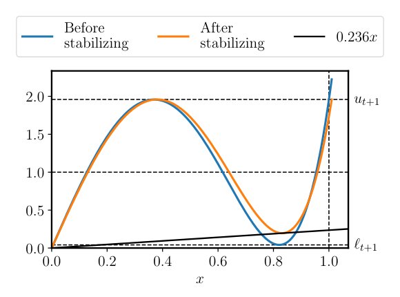
Figure 3: Effects of stabilizing the update rules with a safety factor and cushioning, as described in Section 4.4. The blue curve is the optimal degree-5 polynomial for the interval . It is has numerical issues because it maps singular values near down to almost zero and maps to . The stabilized version is better because it ensures and maps all to at most .
图 3:如第 4.4 节所述,用安全因子和缓冲来稳定更新规则的效果。蓝线是区间 上最优的五次多项式。它有数值问题,因为会把接近 的奇异值映射到几乎为零,并把 映射到约 。稳定后的版本更好,因为它保证 ,并把所有 映射到至多 。
When working in finite-precision arithmetic, especially the half-precision bfloat16 format used in deep learning, we must take some care to avoid blowups and other problems due to numerical error. To this end, we make three small changes to the method. These adjustments stabilize the algorithm with a negligible effect on accuracy. Furthermore, these adjustments can be made in the offline stage by modifying the coefficients of our optimal polynomials.
在有限精度算术中,尤其是深度学习使用的半精度 bfloat16 格式下,必须稍加小心,以免因数值误差出现爆炸或其他问题。为此我们对方法做了三处小改动。这些调整能稳定算法,对精度的影响可以忽略。而且这些调整可以在离线阶段完成,只需修改最优多项式的系数。
The first issue arises when numerical round-off creates singular values that are slightly larger than our current upper bound . Our optimal polynomials converge only when the singular values of are less than . In some cases we have
第一个问题出现在数值舍入制造出略大于当前上界 的奇异值时。我们的最优多项式只有在 的奇异值小于 时才会收敛。有些情况下我们有
so over many iterations, a singular value that is slightly larger than large could grow to instead of converging to .
于是经过许多步之后,一个略大于 的奇异值可能会增长到 ,而不是收敛到 。
To fix this issue, we simply replace each polynomial by . This safety factor corrects for round-off errors in previous iterations while only slightly changing the behavior of the polynomial on the interval , though it does cause the singular values to converge to instead of to . To correct for this, the safety factor can be omitted in the final iteration.
为修复这一问题,我们只需把每个多项式 换成 。这一安全因子能纠正此前各步的舍入误差,同时只轻微改变多项式在区间 上的行为,不过它会让奇异值收敛到 而不是 。为纠正这一点,最后一步可以省去安全因子。
The second issue was identified in [34] and addressed in the context of polynomial iterations by Chen and Chow [11]. In general, iterative methods for aim to increase each singular value relative to the largest singular value; while , after enough iterations, . However, the convergence of each singular value to may not be monotonic. Over the domain , our optimal polynomial oscillates repeatedly between and , so some singular values that are near may get mapped down to . It so happens that this non-monotonicity—even at a single iteration—can cause loss of precision. That is, problems occur if
第二个问题由 [34] 指出,并由 Chen 和 Chow [11] 在多项式迭代的语境下加以处理。一般而言,计算 的迭代法旨在相对于最大奇异值抬升每一个奇异值;虽然 ,足够多步之后会有 。不过每个奇异值向 的收敛未必是单调的。在定义域 上,我们的最优多项式 会在 与 之间反复振荡,因此某些接近 的奇异值可能被映射到 。偏偏这种非单调性——哪怕只出现在单步——就会造成精度损失。也就是说,若
where are singular values of [34]. In the extreme case , the th singular vector will change sign, casuing the method to converge to the polar factor of the wrong matrix. Unlike Newton-Schulz, unscaled Newton, or QDWH, our method is affected by this loss of precision.
就会出问题,其中 是 的奇异值 [34]。在极端情形 时,第 个奇异向量会变号,导致方法收敛到错误矩阵的极因子。与 Newton-Schulz、未缩放的 Newton 或 QDWH 不同,我们的方法会受到这种精度损失的影响。
To mitigate this issue, [11] propose modifying their update polynomials to enforce a lower bound on the ratio . This issue only occurs when ; as , our optimal polynomial approaches the Padé approximant and so for all . We could fully solve the problem by using the Padé approximant instead of our optimal polynomial, but this would significantly slow down convergence. Instead we compromise. When , we find that . Therefore, whenever we select the update rule as though . This change slows convergence, but only very slightly. (The choice of 10 is somewhat arbitrary. In Appendix G, we use a different factor.)
为缓解这一问题,[11] 建议修改更新多项式,给比值 加上一个下界。这一问题只在 时出现;当 时,我们的最优多项式会逼近 Padé 逼近,从而对所有 都有 。我们可以干脆改用 Padé 逼近而不是最优多项式来彻底解决问题,但这会显著拖慢收敛。我们采取折中。当 时,我们发现 。因此只要 ,我们就按 来选择更新规则。这一改动会减慢收敛,但幅度很小。(取 10 多少有些任意。附录 G 中我们使用了不同的因子。)
The third change is copied from the original Muon implementation: normalize by instead of by . As before, we set .
第三处改动照搬自原先的 Muon 实现:用 而不是 来归一化 。和前面一样,我们设 。
4.5 The algorithm
4.5 算法
We give the complete pseudocode for our proposed method for any degree in Algorithm 2. We give the specfic version of the Polar Express with degree and used in our GPT experiments in Algorithm 1. Our algorithm first computes the polynomials of Theorem 4.1 in full precision using the results of Section 4.2 (or the Remez algorithm for ). This stage is offline because the coefficients of the polynomials are only computed and stored once. For every subsequent call to the algorithm, these coefficients are reused and the offline stage is skipped. For instance, in Algorithm 1 these polynomials have been precomputed and stored in the variable coeffs_list.
我们在算法 2 中给出任意次数下所提方法的完整伪代码。算法 1 给出我们在 GPT 实验中使用的、次数 且 的 Polar Express 具体版本。算法首先用第 4.2 节的结果(或当 时用 Remez 算法)在全精度下计算定理 4.1 中的多项式 。这一阶段是离线的,因为多项式系数只需计算并存储一次。此后每次调用算法都会复用这些系数,并跳过离线阶段。例如在算法 1 中,这些多项式已被预先算好并存放在变量 coeffs_list 里。
1: Offline stage: In float64
2: , .
3: for do
4: Solve using Remez Appendix D:
5: .
6: .
7: .
8: end for
9: Online stage: In float16
10: Let .
11: for do
12: .
13: end for
14: return .
Algorithm 2 The General Polar Express
1: 离线阶段: 使用 float64
2: ,。
3: for do
4: 用附录 D 的 Remez 求解:
5: 。
6: 。
7: ,。
8: end for
9: 在线阶段: 使用 float16
10: 令 。
11: for do
12: 。
13: end for
14: return 。
算法 2 一般形式的 Polar Express
The polynomial is then applied to the input matrix in the online stage. The online stage can be performed in lower precision (bfloat16) for greater speed on a GPU. Horner’s rule can be used to carry out each iteration. For instance, if , then
多项式 随后在在线阶段作用于输入矩阵 。在线阶段可以在更低精度(bfloat16)下进行,以便在 GPU 上跑得更快。每一步可以用 Horner 法则来执行。例如,若 ,则
where .
其中 。
A simple implementation of the offline stage of Algorithm 2 is given in Appendix G. For deep learning applications, we recommend using and or with . With these parameters, the offline stage as implemented in Appendix G gives the polynomials encoded in coeffs_list in Algorithm 1. All told, our proposal for Muon is to apply the composition of these polynomials to .
算法 2 离线阶段的一个简单实现见附录 G。对深度学习应用,我们建议取 、 或 ,并取 。在这些参数下,附录 G 中实现的离线阶段会给出算法 1 里 coeffs_list 所编码的那些多项式。总的来说,我们对 Muon 的建议是:把这些多项式的复合作用到 上。
5 Numerical Experiments
5 数值实验
5.1 Convergence of Polar Express
5.1 Polar Express 的收敛
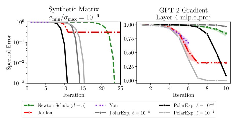
Figure 4: Convergence of various degree-5 polynomial methods in the spectral norm. When tuned properly, Polar Express attains outperforms the other methods at every iteration. Left panel: synthetic matrix with , . Right panel: gradient of a certain weight matrix of a randomly-initialized GPT-2 architecture on a batch of language modeling data, normalized by the Frobenius norm.
图 4:多种五次多项式方法在谱范数下的收敛。调得恰当时,Polar Express 在每一步都超过其他方法。左图:合成矩阵,,。右图:随机初始化的 GPT-2 架构中某一权重矩阵、在一批语言建模数据上的梯度,并按 Frobenius 范数归一化。
We compare the performance of Polar Express against degree-5 Newton-Schulz and the methods of Chen and Chow [11], Jordan [22], and You [9].
我们将 Polar Express 与五次 Newton-Schulz,以及 Chen 和 Chow [11]、Jordan [22]、You [9] 的方法进行比较。
We first study an idealized scenario where the spectrum of the input matrix is known exactly. We generate a random matrix whose singular values are evenly spaced on a logarithmic scale between and . The right and left singular vectors are chosen at random. The left panel of Figure 4 shows the results. Since all the methods in this plot use degree-5 polynomials, their computational and runtime costs are all proportional to the number of iterations. As expected, Newton-Schulz converges but makes almost no progress for the first 17 iterations. Jordan’s method rapidly achieves an error of after just 11 iterations, but ceases to converge further. You’s method, which is difficult to see on the plot because it is only defined for six iterations, converges at a similar rate as Jordan’s method. When Polar Express is instantiated with , it dominates the other methods at every iteration, achieving excellent accuracy after just 11 iterations and converging about twice as fast as Newton-Schulz to any given error. Even when the lower bound on is wrong by two orders of magnitude in either direction, the method remains competitive, though it does not actually outperform Keller until iteration 13 or 14.
我们首先研究输入矩阵的谱已知的理想情形。我们生成一个随机矩阵,其奇异值在 与 之间按对数均匀间隔排列。左、右奇异向量随机选取。图 4 左图给出结果。由于图中所有方法都使用五次多项式,它们的计算量和运行时间都与迭代次数成正比。如所预期,Newton-Schulz 会收敛,但前 17 步几乎没有进展。Jordan 的方法只需 11 步就能迅速把误差降到约 ,但之后不再继续收敛。You 的方法在图上不容易看清,因为它只定义了六步,收敛速度与 Jordan 的方法相近。当 Polar Express 取 时,它在每一步都压过其他方法,只需 11 步就能达到很高的精度,并且收敛到任意给定误差的速度大约是 Newton-Schulz 的两倍。即便对 下界的猜测在任一方向偏了两个数量级,该方法仍然具有竞争力,不过要到第 13 或 14 步才真正超过 Keller。
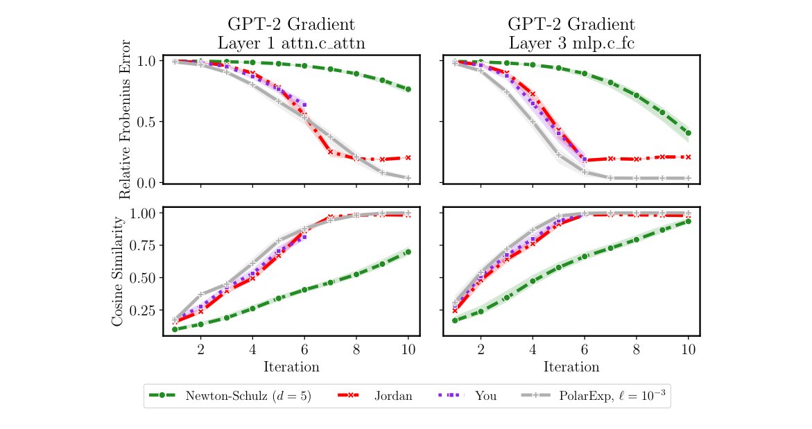
Figure 5: Convergence of polynomial methods in the Frobenius norm on GPT-2 gradient matrices. The number of matrix-matrix products is , where is the degree ( for Chen & Chow; for all others) and is the number of iterations.
图 5:多项式方法在 GPT-2 梯度矩阵上、按 Frobenius 范数衡量的收敛。矩阵-矩阵乘法次数为 ,其中 为次数(Chen & Chow 为 ,其余均为 ), 为迭代次数。
Next we test the methods’ performance on a matrix from a real-world application, namely, the gradient of a weight matrix from the fourth transformer block of a GPT-2 architecture with respect to a language modeling objective on a batch of text from the Tiny Shakespeare dataset [24]. The right panel of Figure 4 shows the results. Once again, the best-tuned version of Polar Express outperforms the other methods. This time, we see that setting to be many orders of magnitude too small can delay convergence significantly, and make Polar Express less competitive as compared to Jordan’s method.
接下来我们在一个真实应用中的矩阵上测试这些方法的表现,即某个 GPT-2 架构第四个 Transformer 块中一个权重矩阵、相对于 Tiny Shakespeare 数据集 [24] 一批文本上的语言建模目标的梯度。图 4 右图给出结果。再一次,调得最好的 Polar Express 超过了其他方法。这一次我们看到,若把 设得比真实值小许多个数量级,会显著推迟收敛,并使 Polar Express 相对 Jordan 方法的竞争力下降。
For most other weight matrices in this GPT-2 model, the methods all take more than 10 iterations to converge in the spectral norm. The spectral error is large if there is even one outlying singular value that is far from . However, for some applications, we may be satisfied with a weaker notion of convergence, like the relative Frobenius norm. Figure 5 shows the performance of various methods on this metric. We use gradient matrices of the same model, but from two different layers. In addition, we compare the degree-5 methods to Chen and Chow’s degree-3 method. To make this comparison fair, we measure the number of matrix-matrix products performed by each method instead the number of iterations. We find that Polar Express can once again dominate the other methods across iterations. Chen and Chow’s method is also quite competitive, and the remaining methods behave much as in Figure 4.
对该 GPT-2 模型中的大多数其他权重矩阵,这些方法都需要超过 10 步才能在谱范数下收敛。哪怕只有一个远离 的离群奇异值,谱误差也会很大。不过对某些应用,我们也许满足于更弱的收敛概念,例如相对 Frobenius 范数。图 5 展示了各方法在这一度量上的表现。我们使用同一模型、但来自两个不同层的梯度矩阵。此外,我们把五次方法与 Chen 和 Chow 的三次方法相比较。为使比较公平,我们统计每种方法执行的矩阵-矩阵乘法次数,而不是迭代次数。我们发现 Polar Express 可以再次在各步都压过其他方法。Chen 和 Chow 的方法也相当有竞争力,其余方法的表现则与图 4 大致相同。
5.2 Training GPT-2
5.2 训练 GPT-2
In our final experiment, we compare the performance of using our Polar Express method given in Algorithm 1 inside the Muon algorithm versus Jordan’s [22] and You’s [9] methods.
在最后一组实验中,我们比较把算法 1 给出的 Polar Express 方法放进 Muon 算法,与使用 Jordan [22] 和 You [9] 的方法时的表现。
Our experimental setup is based on the modified nanogpt code of Jordan [21]. We train two different GPT-2 models:
实验设置基于 Jordan 修改过的 nanogpt 代码 [21]。我们训练两种不同的 GPT-2 模型:
and a vocabulary size of , using a context length of . Training is performed on 1B tokens from the FineWeb dataset [2], using a batch size of 32 and a single epoch. All models are trained with mixed precision (bfloat16) on 4 H100 GPUs. For all methods we use the learning rate schedule proposed in [21], consisting of a constant phase for the first 40% of training steps followed by a linear decay. All methods for the matrix sign computations are performed in float16b precision and use five iterations.
词表大小为 ,上下文长度为 。训练在 FineWeb 数据集 [2] 的 10 亿 token 上进行,批大小为 32,训练一个 epoch。所有模型都在 4 张 H100 GPU 上以混合精度(bfloat16)训练。对所有方法我们都采用 [21] 提出的学习率日程:前 40% 训练步保持恒定,随后线性衰减。所有矩阵符号计算都在 float16b 精度下进行,并使用五步迭代。
We apply Muon selectively to certain layers of the model. Following the nano-gpt implementation [21], we assign Muon to all parameters with at least two dimensions (typically weight matrices, and excluding RMS norm parameters), excluding the embeddings, unembeddings, and the attention head. These excluded parameters are instead optimized with AdamW.
我们对模型的某些层有选择地使用 Muon。沿用 nano-gpt 的实现 [21],我们把 Muon 分配给所有至少两维的参数(通常是权重矩阵,并排除 RMS 归一化参数),同时排除嵌入、反嵌入以及注意力头。这些被排除的参数改用 AdamW 优化。
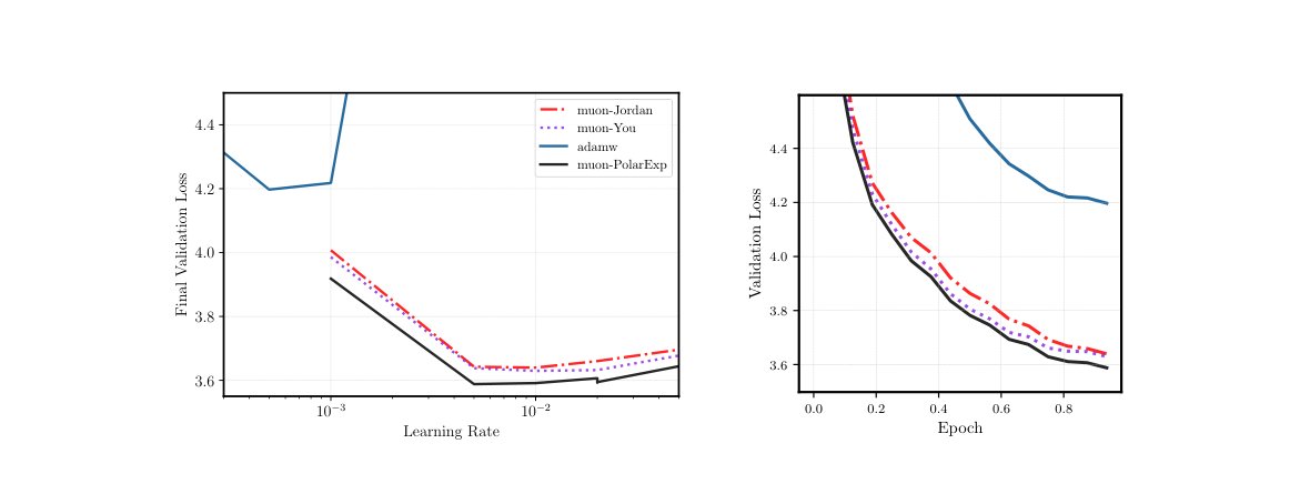
Figure 6: Training a GPT-2 (124M) model on 1 Billion tokens of the Fineweb data set [2]. The Legend muon- refers to using muon with the method for computing . Top Left: The final validation loss vs. the learning rate. The final best validation losses for each method were, in reverse order, adamw: , muon-Jordan: , muon-You: and muon-PolarExp: . Bottom Left: The final training loss vs the learning rate. Top Right: Validation loss vs. number of iterations. Bottom Left: validation loss vs. time, plotting each method with its best learning rate.
图 6:在 Fineweb 数据集 [2] 的 10 亿 token 上训练 GPT-2(124M)模型。图例 muon- 表示用 方法计算 来实现 muon。左上:最终验证损失与学习率。各方法最终最好的验证损失从差到好依次为 adamw:,muon-Jordan:,muon-You:,muon-PolarExp:。左下:最终训练损失与学习率。右上:验证损失与迭代次数。左下:验证损失与时间,每种方法取其最优学习率作图。
Figure 1 and Figure 6 shows the resulting runs of each method in terms of validation loss and training loss on the GPT-Large and GPT-Small models, respectively. In both figures we can see that muon-PolarExp achieves a better validation and training loss than muon-Jordan or muon-You for every learning rate. Since each iteration of the different matrix sign methods are equally expensive (since they all apply a degree 5 polynomial), improved validation loss in terms of epochs also translates to an improved loss in terms of wall clock time (see bottom right of Figure 6). The advantage is remarkably consistent across all learning rates and epochs.
图 1 和图 6 分别给出各方法在 GPT-Large 和 GPT-Small 模型上、按验证损失和训练损失衡量的运行结果。两图都可以看到,对每一个学习率,muon-PolarExp 的验证损失和训练损失都优于 muon-Jordan 或 muon-You。由于不同矩阵符号方法的每一步代价相同(它们都作用一个五次多项式),按 epoch 衡量的验证损失改进,也会转化成按墙钟时间衡量的损失改进(见图 6 右下)。这一优势在所有学习率和所有 epoch 上都非常稳定。
References
参考文献
[1] N. I. Achieser. Theory of approximation . Dover Publications, Inc., New York, 1992. Translated from the Russian and with a preface by Charles J. Hyman, Reprint of the 1956 English translation.
[2] Samuel Aroca-Ouellette, Philippe Beaudoin, Guillaume Lajoie, Liam Paull, Joelle Pineau, Pascal Vincent, and Anirudh Goyal. Fineweb: Learning language models with high quality web data. In NeurIPS Datasets and Benchmarks Track , 2023. URL: https://arxiv.org/abs/2306.03061 .
[3] Michele Benzi and Ru Huang. Some matrix properties preserved by generalized matrix functions. Spec. Matrices , 7:27–37, 2019. doi:10.1515/spma-2019-0003 .
[4] Jeremy Bernstein and Laker Newhouse. Modular duality in deep learning. arXiv preprint arXiv:2410.21265 , 2024. URL: https://arxiv.org/abs/2410.21265 .
[5] Jeremy Bernstein and Laker Newhouse. Old optimizer, new norm: An anthology. arXiv preprint arXiv:2409.20325 , 2024. URL: https://arxiv.org/abs/2409.20325 .
[6] Ȧ. Björck and C. Bowie. An iterative algorithm for computing the best estimate of an orthogonal matrix. SIAM J. Numer. Anal. , 8:358–364, 1971. doi:10.1137/0708036 .
[7] Christos Boutsikas, Petros Drineas, and Ilse C. F. Ipsen. Small singular values can increase in lower precision. SIAM J. Matrix Anal. Appl. , 45(3):1518–1540, 2024. doi:10.1137/23M1557209 .
[8] J Douglas Carroll and Phipps Arabie. Multidimensional scaling. pages 179–250, 1998. URL: https://www.sciencedirect.com/science/article/pii/B9780120999750500051 , doi:10.1016/B978-012099975-0.50005-1 .
[9] Franz Louis Cesista, You Jiacheng, and Keller Jordan. Squeezing 1-2% efficiency gains out of muon by optimizing the newton-schulz coefficients, 2025. URL: http://leloykun.github.io/ponder/muon-opt-coeffs/ .
[10] PL Chebyshev. Questions on smallest quantities connected with the approximate representation of functions (1859). Collected works , 2:151–235, 1947.
[11] Jie Chen and Edmond Chow. A stable scaling of newton-schulz for improving the sign function computation of a hermitian matrix. Preprint ANL/MCS-P5059-0114 , 2014. URL: https://www.mcs.anl.gov/papers/P5059-0114.pdf .
[12] E. W. Cheney. Introduction to approximation theory . McGraw-Hill Book Co., New York-Toronto-London, 1966.
[13] John Duchi, Elad Hazan, and Yoram Singer. Adaptive subgradient methods for online learning and stochastic optimization. J. Mach. Learn. Res. , 12:2121–2159, 2011.
[14] Alexandre Eremenko and Peter Yuditskii. Uniform approximation of sgn x {\rm sgn},x by polynomials and entire functions. J. Anal. Math. , 101:313–324, 2007. doi:10.1007/s11854-007-0011-3 .
[15] Gene H. Golub and Charles F. Van Loan. Matrix computations . Johns Hopkins Studies in the Mathematical Sciences. Johns Hopkins University Press, Baltimore, MD, fourth edition, 2013.
[16] J. C. Gower and G. B. Dijksterhuis. Procrustes problems , volume 30 of Oxford Statistical Science Series . Oxford University Press, Oxford, 2004. doi:10.1093/acprof:oso/9780198510581.001.0001 .
[17] Vineet Gupta, Tomer Koren, and Yoram Singer. Shampoo: Preconditioned stochastic tensor optimization. In Jennifer Dy and Andreas Krause, editors, Proceedings of the 35th International Conference on Machine Learning , volume 80 of Proceedings of Machine Learning Research , pages 1842–1850. PMLR, 10–15 Jul 2018. URL: https://proceedings.mlr.press/v80/gupta18a.html .
[18] Nicholas J. Higham. Computing the polar decomposition—with applications. SIAM J. Sci. Statist. Comput. , 7(4):1160–1174, 1986. doi:10.1137/0907079 .
[19] Nicholas J. Higham. Functions of matrices . SIAM, Philadelphia, PA, 2008. doi:10.1137/1.9780898717778 .
[20] Elias Jarlebring and Gustaf Lorentzon. The polynomial set associated with a fixed number of matrix-matrix multiplications. arXiv preprint arXiv:2504.01500 , 2025. URL: https://arxiv.org/abs/2504.01500 .
[21] Keller Jordan, Jeremy Bernstein, Brendan Rappazzo, @fernbear.bsky.social, Boza Vlado, You Jiacheng, Franz Cesista, Braden Koszarsky, and @Grad62304977. modded-nanogpt: Speedrunning the nanogpt baseline, 2024. URL: https://github.com/KellerJordan/modded-nanogpt .
[22] Keller Jordan, Yuchen Jin, Vlado Boza, Jiacheng You, Franz Cesista, Laker Newhouse, and Jeremy Bernstein. Muon: An optimizer for hidden layers in neural networks, 2024. URL: https://kellerjordan.github.io/posts/muon/ .
[23] Tetsuya Kaneko, Simone Fiori, and Toshihisa Tanaka. Empirical arithmetic averaging over the compact Stiefel manifold. IEEE Trans. Signal Process. , 61(4):883–894, 2013. doi:10.1109/TSP.2012.2226167 .
[24] Andrej Karpathy. char-rnn. https://github.com/karpathy/char-rnn , 2015.
[25] Charles Kenney and Alan J. Laub. Rational iterative methods for the matrix sign function. SIAM J. Matrix Anal. Appl. , 12(2):273–291, 1991. doi:10.1137/0612020 .
[26] Diederik P. Kingma and Jimmy Ba. Adam: A method for stochastic optimization. In International Conference on Learning Representations , 2015. URL: http://arxiv.org/abs/1412.6980 .
[27] Zdislav Kovářík. Some iterative methods for improving orthonormality. SIAM J. Numer. Anal. , 7:386–389, 1970. doi:10.1137/0707031 .
[28] Eunsang Lee, Joon-Woo Lee, Jong-Seon No, and Young-Sik Kim. Minimax approximation of sign function by composite polynomial for homomorphic comparison. IEEE Transactions on Dependable and Secure Computing , 19(6):3711–3727, 2022. doi:10.1109/TDSC.2021.3105111 .
[29] R. B. Leipnik. Rapidly convergent recursive solution of quadratic operator equations. Numer. Math. , 17:1–16, 1971. doi:10.1007/BF01395861 .
[30] Jingyuan Liu, Jianlin Su, Xingcheng Yao, Zhejun Jiang, Guokun Lai, Yulun Du, Yidao Qin, Weixin Xu, Enzhe Lu, Junjie Yan, et al. Muon is scalable for LLM training. arXiv preprint arXiv:2502.16982 , 2025. URL: https://arxiv.org/abs/2502.16982 .
[31] Ilya Loshchilov and Frank Hutter. Decoupled weight decay regularization. In International Conference on Learning Representations , 2019. URL: https://openreview.net/forum?id=Bkg6RiCqY7 .
[32] Yuji Nakatsukasa, Zhaojun Bai, and François Gygi. Optimizing Halley’s iteration for computing the matrix polar decomposition. SIAM J. Matrix Anal. Appl. , 31(5):2700–2720, 2010. doi:10.1137/090774999 .
[33] Yuji Nakatsukasa and Roland W. Freund. Computing fundamental matrix decompositions accurately via the matrix sign function in two iterations: the power of Zolotarev’s functions. SIAM Rev. , 58(3):461–493, 2016. doi:10.1137/140990334 .
[34] Yuji Nakatsukasa and Nicholas J. Higham. Backward stability of iterations for computing the polar decomposition. SIAM J. Matrix Anal. Appl. , 33(2):460–479, 2012. doi:10.1137/110857544 .
[35] Yuji Nakatsukasa and Nicholas J. Higham. Stable and efficient spectral divide and conquer algorithms for the symmetric eigenvalue decomposition and the SVD. SIAM J. Sci. Comput. , 35(3):A1325–A1349, 2013. doi:10.1137/120876605 .
[36] Herbert Neuberger. Exactly massless quarks on the lattice. Phys. Lett. B , 417(1-2):141–144, 1998. doi:10.1016/S0370-2693(97)01368-3 .
[37] Ricardo Pachón and Lloyd N. Trefethen. Barycentric-Remez algorithms for best polynomial approximation in the chebfun system. BIT , 49(4):721–741, 2009. doi:10.1007/s10543-009-0240-1 .
[38] T Parks and James McClellan. Chebyshev approximation for nonrecursive digital filters with linear phase. IEEE Transactions on circuit theory , 19(2):189–194, 1972. doi:10.1109/TCT.1972.1083419 .
[39] Michael S. Paterson and Larry J. Stockmeyer. On the number of nonscalar multiplications necessary to evaluate polynomials. SIAM J. Comput. , 2:60–66, 1973. doi:10.1137/0202007 .
[40] Thomas Pethick, Wanyun Xie, Kimon Antonakopoulos, Zhenyu Zhu, Antonio Silveti-Falls, and Volkan Cevher. Training deep learning models with norm-constrained lmos, 2025. URL: https://arxiv.org/abs/2502.07529 , arXiv:2502.07529 .
[41] Artem Riabinin, Egor Shulgin, Kaja Gruntkowska, and Peter Richtárik. Gluon: Making muon & scion great again! (bridging theory and practice of lmo-based optimizers for llms), 2025. URL: https://arxiv.org/abs/2505.13416 , arXiv:2505.13416 .
[42] Ishaan Shah, Anthony M Polloreno, Karl Stratos, Philip Monk, Adarsh Chaluvaraju, Andrew Hojel, Andrew Ma, Anil Thomas, Ashish Tanwer, Darsh J Shah, et al. Practical efficiency of muon for pretraining. arXiv preprint arXiv:2505.02222 , 2025. URL: https://arxiv.org/abs/2505.02222 .
[43] Hao-Jun Michael Shi, Tsung-Hsien Lee, Shintaro Iwasaki, Jose Gallego-Posada, Zhijing Li, Kaushik Rangadurai, Dheevatsa Mudigere, and Michael Rabbat. A distributed data-parallel PyTorch implementation of the distributed Shampoo optimizer for training neural networks at-scale. arXiv preprint arXiv:2309.06497 , 2023. URL: https://arxiv.org/abs/2309.06497 .
[44] Modula Systems. Newton-schulz algorithm — jiacheng’s six-step method. https://docs.modula.systems/algorithms/newton-schulz/#jiacheng-s-six-step , 2024. Accessed: 2025-05-19.
[45] Attila Szabo and Neil S Ostlund. Modern quantum chemistry: introduction to advanced electronic structure theory . Courier Corporation, 1996.
[46] Lloyd N. Trefethen. Approximation theory and approximation practice . Society for Industrial and Applied Mathematics (SIAM), Philadelphia, PA, extended edition, 2020.
[47] Nikhil Vyas, Depen Morwani, Rosie Zhao, Itai Shapira, David Brandfonbrener, Lucas Janson, and Sham M. Kakade. SOAP: Improving and stabilizing shampoo using adam for language modeling. In The Thirteenth International Conference on Learning Representations , 2025. URL: https://openreview.net/forum?id=IDxZhXrpNf .
[48] Greg Yang, James B. Simon, and Jeremy Bernstein. A spectral condition for feature learning, 2024. URL: https://arxiv.org/abs/2310.17813 , arXiv:2310.17813 .
[49] Zhenyue Zhang, Hongyuan Zha, and Wenlong Ying. Fast parallelizable methods for computing invariant subspaces of Hermitian matrices. J. Comput. Math. , 25(5):583–594, 2007. URL: http://www.jstor.org/stable/43693395 .
Appendix A Proof of Theorem 4.1
附录 A 定理 4.1 的证明
The aim of this section is to prove Theorem 4.1. We begin with a result that provides a few essential properties for the the polynomial solving (7) when . This result is known as Chebyshev’s theorem [10] or the equioscillation theorem [46, Chapter 10].
本节旨在证明定理 4.1。我们先给出一个结果,它提供当 时求解 (7) 的多项式的若干基本性质。该结果称为 Chebyshev 定理 [10],或等振荡定理 [46, 第 10 章]。
A.1.
Let and . Consider the problem
A.1。
设 且 。考虑问题
There exists a unique polynomial solving (16). Furthermore, is the unique solution to the above problem if and only if there exist distinct points such that
存在唯一的多项式 求解 (16)。此外, 是上述问题的唯一解,当且仅当存在 个互异的点 使得
for or .
其中 或 。
Proof.
A discussion can be found in [14]. Here we include a formal proof for completeness.
证明。
相关讨论见 [14]。这里为完整起见给出一个形式证明。
By Chebyshev’s Theorem [1, 10, 12] it is sufficient to show that satisfies the Haar condition: any non-zero can have at most roots in .
由 Chebyshev 定理 [1, 10, 12],只需证明 满足 Haar 条件:任意非零 在 内至多有 个根。
Since we know that can have at most roots in . However, since and we know that has one root at zero, and the remaining roots come in symmetric pairs . Because of this, can have at most roots in the positive orthant, and thus it can have at most roots in . Hence, satisfies the Haar condition, which yields the desired result.
由于 ,我们知道 在 上至多有 个根。不过,由于 且 ,我们知道 在零点有一个根,其余根成对称对 出现。因此, 在正半轴上至多有 个根,从而在 内至多有 个根。于是 满足 Haar 条件,这就给出了所需结果。
∎
The proof of Theorem 4.1 will be by induction on . We begin by establishing the base case, , which is handled by the following result.
定理 4.1 的证明将对 做归纳。我们先建立基础情形 ,由下面的结果处理。
A.2.
Let and define
A.2。
设 并定义
Then
则
Proof.
Throughout the proof we assume . We begin with proving
证明。
整个证明中我们假定 。我们先证明
Consider the polynomial . The proof will contain three steps. We first rule out the trivial case that , since would then be a better approximation. Hence, cannot be the zero polynomial.
考虑多项式 。证明分三步。我们先排除 为零多项式这一平凡情形,因为否则 会是更好的逼近。因此 不可能是零多项式。
Step 1: has exactly stationary points inside the open interval .
第一步: 在开区间 内恰好有 个驻点。
Note that has at most stationary points in , since its derivative is a polynomial of degree . Furthermore, since is odd, we have that is even of degree , and thus can have at most stationary points contained in . Hence, there can be at most stationary points of inside the interval .
注意 在 上至多有 个驻点,因为它的导数 是次数为 的多项式。此外,由于 是奇函数,我们有 是次数为 的偶函数,因而在 内至多有 个驻点。因此 在区间 内至多有 个驻点。
By Lemma A.1 there are points where is maximized or minimized in . These points are either stationary points or they are endpoints of the interval . Let be the number of stationary points and be the number of endpoints in the set . Since a point can be both a stationary point and an endpoint we have . However, and , which follows from the previous paragraph where we showed that there are at most stationary points of in . So , and consequently we must have and , as required.
由引理 A.1,存在 个点 ,使 在 上在这些点取到极大或极小。这些点要么是驻点,要么是区间 的端点。设 为驻点个数, 为集合 中端点的个数。由于一个点可以既是驻点又是端点,我们有 。不过 且 ,这来自上一段我们证明的、 在 内至多有 个驻点。于是 ,因而必须有 且 ,此即所需。
Step 2: is a maximum of on the interval
第二步: 是 在区间 上的一个极大点
By Lemma A.1 and the discussion from Step 1, we know that is maximized at points inside and of these points are contained inside the open interval . Hence, must either be a maximum or a minimum of . We will show that must be a maximum by contradiction.
由引理 A.1 以及第一步的讨论,我们知道 在 内的 个点上取到最大值,且其中 个点落在开区间 内。因此 必须是 的一个极大或极小。我们将用反证法证明 必须是极大。
Suppose was a minimum of on . First note that is trivially non-negative on , or else would be a better polynomial. Hence, since we must have for some , or else the zero polynomial would be a better approximation. Hence, for some we have .
假设 是 在 上的一个极小。首先注意 在 上显然非负,否则 会是更好的多项式。因此,由于 ,对某个 必须有 ,否则零多项式 会是更好的逼近。于是对某个 有 。
We must also have or else is not a minimum of . Since for some and , by the intermediate value theorem there exists a point such that . However, by the discussion above we know that all stationary points of are contained inside the open interval . Hence, cannot be a minimum of on . However, by Step 1 we know that the endpoints of must be either minima or maxima of . Hence, is a maximum of on .
我们还必须有 ,否则 就不是 的极小。既然对某个 有 且 ,由介值定理存在一点 使得 。但由上面的讨论,我们知道 的所有驻点都落在开区间 内。因此 不可能是 在 上的极小。然而由第一步我们知道 的端点必须是 的极小或极大。因此 是 在 上的一个极大。
Step 3: Obtaining the desired equalities
第三步:得到所需的等式
Since has a maximum in at , we have . The other two equalities are immediate consequences of the equioscillation property of Lemma A.1 and that is a minimum of over the set . ∎
由于 在 上于 取到极大,我们有 。另外两个等式是 的等振荡性质(引理 A.1)以及 是 在集合 上的极小这一事实的直接推论。∎
With the above-mentioned result in hand, we are ready to prove Theorem 4.1.
有了上述结果,我们就可以证明定理 4.1。
See 4.1
见 4.1
Proof.
The proof of (10) is an immediate consequence of Lemma A.2, since for each , is the optimal approximation in to .
证明。
(10) 的证明是引理 A.2 的直接推论,因为对每个 , 都是 中对 的最优逼近。
We now proceed with the proof of (11), which will be by induction. The proof for is an immediate consequence of Lemma A.2 and we also have by (10). Now suppose the result is true for all . For , note that the image of on is exactly by i). Hence, if we define , then the image of on is . Furthermore, by i) we also have . Pick any such that and
我们接着用归纳法证明 (11)。 时的证明是引理 A.2 的直接推论,并且由 (10) 还有 。现在假设结果对所有 成立。对 ,注意 在 上的像恰好是 ,这由 i) 得出。因此,若定义 ,则 在 上的像是 。此外,由 i) 还有 。任取满足 且
for some . Let the image of on be . We will prove that by contradiction.
的 ,其中 。设 在 上的像为 。我们将用反证法证明 。
Suppose . Define . Then, the image of the scaled function on is and satisfies
假设 。定义 。则缩放后的函数 在 上的像是 ,并且 满足
Recall by our inductive hypothesis, we have where the second equality holds by (10). It follows that
回忆由归纳假设,我们有 ,其中第二个等号由 (10) 成立。于是
which leads to a contradiction to our inductive hypothesis that is optimal. Hence, we must have .
这与归纳假设中 为最优相矛盾。因此必须有 。
Consequently, using that , we will show that for any and for any cannot be a better approximation than . In particular, we have
于是,利用 ,我们将证明对任意 以及任意 , 都不可能比 更好。具体来说,我们有
where the second and third equality follow by changing variables so that
其中第二、第三个等号来自变量替换 ,从而
and this last equality follows because the space is invariant under input rescaling; that is, for any , the map preserves the space . This concludes the proof. ∎
而最后一个等号成立,是因为空间 在输入缩放下不变;也就是说,对任意 ,映射 保持空间 。这就完成了证明。∎
Appendix B Proof of Theorem 4.3
附录 B 定理 4.3 的证明
In this section we provide the proof of the convergence guarantee stated in Theorem 4.3.
本节给出定理 4.3 中所述收敛保证的证明。
See 4.3
见 4.3
Proof.
Define
证明。
定义
$$p^{\star}=\argmin_{\begin{subarray}{c}p=p_{T}\circ p_{T-1}\circ\cdots\circ p_{1}\
p_{t}\in\mathbb{P}{d}^{*}\end{subarray}},\max{x\in[\ell,u]}\left|1-p(x)\right|.$$
Then Algorithm 2 returns . Let be Padé-approximant to [25, Section 3] and define . Define as the composition of with itself times. Then, by Theorem 4.1 and [25, Theorem 3.1] we have
则算法 2 返回 。设 为对 的 Padé 逼近 [25, 第 3 节],并定义 。定义 为 与自身复合 次。则由定理 4.1 和 [25, 定理 3.1] 我们有
as required. ∎
此即所需。∎
Appendix C Proof of equivalence between (6) and (7)
附录 C (6) 与 (7) 等价性的证明
In this section we provide a proof for the equivalence between (6) and (7). It is sufficient to show that for any fixed polynomial we have
本节给出 (6) 与 (7) 等价性的证明。只需证明对任意固定的多项式 都有
$$\varepsilon_{1}:=\max_{\begin{subarray}{c}\bm{M}\in\mathbb{R}^{m\times n}\
\sigma(\bm{M})\subset[\ell,u]\end{subarray}}\left|\polar(\bm{M})-p(\bm{M})\right|{2}=\max{x\in[\ell,u]}\left|1-p(x)\right|:=\varepsilon_{2}.$$
For any fixed , by the unitary invariance of the spectral norm we immediately have
对任意固定的 ,由谱范数的酉不变性我们立刻有
Consequently, .
因此 。
Suppose that is chosen so that Without loss of generality, assume . Letting , for any matrix and with orthonormal columns, and noting yields
设 使得 。不失一般性,假定 。令 ,其中任意矩阵 和 具有标准正交列,并注意到 ,便得到
Consequently, . Hence, , as desired.
因此 。于是 ,此即所需。
Appendix D Remez algorithm
附录 D Remez 算法
Theorem 4.1 shows that we can solve (7) by greedily choosing the optimal approximation for each interval for . In this section, we outline how the Remez algorithm [37, 38] can be used to approximate .
定理 4.1 表明,只要对每个区间 ()贪心地选择最优逼近 ,就能求解 (7)。本节概述如何用 Remez 算法 [37, 38] 来逼近 。
We begin with the case when . In this case, there is a simple closed form for the optimal odd polynomial ; see [11]. On a given interval , the optimal approximation to the constant function is given by the scaled and shifted Newton-Schulz polynomial :
我们从 的情形开始。这时最优奇次多项式 有简单的闭式;见 [11]。在给定区间 上,对常值函数 的最优逼近由缩放并平移后的 Newton-Schulz 多项式 给出:
One can verify that this polynomial satisfies the equioscillation condition from Lemma A.1 at and therefore necessarily has to be the optimal approximation from . Unfortunately, for larger finding closed form expressions for optimal approximations from becomes challenging. In fact, to the best of our knowledge the optimal approximation is not known for . However, we can approximate the optimal polynomial using the Remez algorithm.
可以验证该多项式在 处满足引理 A.1 的等振荡条件,因而必然是来自 的最优逼近。可惜对更大的 ,要为来自 的最优逼近找到闭式变得困难。事实上,据我们所知,当 时最优逼近并不已知。不过我们可以用 Remez 算法来逼近最优多项式。
Let . Recall that from Lemma A.1 the optimal polynomial must satisfy the equioscillation property times. The Remez algorithm is an iterative algorithm that finds the equioscillation points from Lemma A.1 by iteratively refining a sequence of trial points so that converges to . From the sequence of trial points the algorithm also finds a sequence of polynomials so that converges to the optimal polynomial. The convergence is extremely fast, and usually 10 iterations is sufficient to converge to the optimal polynomial up to double precision machine epsilon [37]. More commonly, the Remez algorithm is used to find optimal polynomial approximations to general continuous functions where or even . However, because the polynomial we build to approximate is a composition of polynomials, each of which has a low degree, in our setting the degree is small, usually . For the Remez algorithm simplifies significantly. We now describe this simplified algorithm.
设 。回忆引理 A.1,最优多项式必须满足 次等振荡性质。Remez 算法是一种迭代算法,它通过不断修正一列试验点 ,使其收敛到引理 A.1 中的等振荡点集 。从试验点列 出发,算法同时找到一列多项式 ,使其收敛到最优多项式。收敛极快,通常 10 步就足以收敛到双精度机器 epsilon 意义下的最优多项式 [37]。更常见的是,Remez 算法被用来寻找对一般连续函数的最优多项式逼近,其中 甚至 。不过,由于我们用来逼近 的多项式是若干低次多项式的复合,在我们的设定中次数 很小,通常 。对 ,Remez 算法会显著简化。我们接下来描述这一简化算法。
Recall that as stated in Lemma A.1, the unique optimal approximation satisfies the equioscillation property at four points. The Remez algorithm first starts with a trial set which ideally should come close to satisfying the equioscillation property. Since we know that and must be equioscillation points we always set and for all . and are chosen to be and , since we observe that as these are approximately the other equioscillation points. Next, the algorithm solves the following system of equations
回忆引理 A.1 所述,唯一的最优逼近 在四个点处满足等振荡性质。Remez 算法首先从一个试验集 出发,该集合理想情况下应接近满足等振荡性质。既然我们知道 和 必须是等振荡点,我们始终令所有 都有 和 。 和 取为 和 ,因为我们观察到当 时它们大致就是其余等振荡点。接下来,算法求解下列方程组
for the unknowns and . Recalling that and , (17) can equivalently be written as a system of linear equations
未知数为 和 。回忆 且 ,(17) 可以等价地写成线性方程组
$$\begin{bmatrix}\ell&\ell^{3}&\ell^{5}&1\
x_{1}^{(1)}&(x_{1}^{(1)})^{3}&(x_{1}^{(1)})^{5}&-1\
x_{2}^{(1)}&(x_{2}^{(1)})^{3}&(x_{2}^{(1)})^{5}&1\
u&u^{3}&u^{5}&-1\end{bmatrix}\begin{bmatrix}a\
b\
c\
E\end{bmatrix}=\begin{bmatrix}1\
1\
1\
1\end{bmatrix}. \tag{18}$$
Once we have solved for and we set . Now we want to find the error in the norm of using to approximate . We therefore find local maxima of the error function on by setting the derivative of to zero and solving for . This results in the quartic equation , which has closed form solutions given by the quadratic formula after the substitution . We now let and be the solutions to this equation and let . We repeat the procedure until .
一旦解出 和 ,我们就令 。现在我们要找出用 逼近 时的 范数误差。因此我们令误差函数 的导数为零并求解 ,以找出它在 上的局部极大。这给出四次方程 ,在替换 后可用二次公式给出闭式解。我们现在令 和 为该方程的解,并令 。我们重复这一过程,直到 。
We note that the matrix appearing in (18) is a Vandermonde matrix. Vandermonde matrices become notoriously ill-conditioned as the degree grows large [15, Section 4.6]. However, since in our setting we choose to be small, there is no ill-conditioning. Instead, we observe ill-conditioning when . However, as the optimal polynomial will converge to the polynomial , which can be verified by noting that as all equioscillation points must converge to . For general , the polynomial will converge to where is the Padé approximant to [25]. In fact, this polynomial is extremely close to the optimal polynomial for sufficiently large . To see this, let be the optimal approximation from and let . Then,
我们注意到 (18) 中出现的矩阵是 Vandermonde 矩阵。当次数变大时,Vandermonde 矩阵会变得出了名地病态 [15, 第 4.6 节]。不过在我们的设定中 取得很小,因此没有病态问题。相反,我们在 时观察到病态。但当 时,最优多项式会收敛到多项式 ,这一点可以通过注意到当 时所有等振荡点 都必须收敛到 来验证。对一般的 ,多项式会收敛到 ,其中 是对 的 Padé 逼近 [25]。事实上,当 足够大时,这一多项式与最优多项式极为接近。为看清这一点,设 为来自 的最优逼近,并设 。则
where we invoked [25, Theorem 3.1] and the fact that is the optimal approximation to from . Hence, when , where is the double precision machine epsilon, then . In other words, up to double precision machine epsilon, is equal to . Therefore, whenever the algorithm simply returns as the optimal polynomial.
其中我们援引了 [25, 定理 3.1],以及 是来自 的对 的最优逼近这一事实。因此,当 时——这里 是双精度机器 epsilon——就有 。换句话说,在双精度机器 epsilon 的意义下, 等于 。因此,只要 ,算法就直接返回 作为最优多项式。
The algorithm is outlined in Algorithm 3. In our experiments, we never observed Algorithm 3 taking more than five iterations to converge.
算法概述于算法 3。在我们的实验中,从未观察到算法 3 需要超过五步才能收敛。
define
if then
Return
end if
,
while do
end while
Return
Algorithm 3 Remez algorithm (degree 5 approximation for )
define
if then
Return
end if
,
while do
,
end while
Return
算法 3 Remez 算法(对 的五次逼近)
Appendix E Initialization for Matrices with Large Spectral Gaps
附录 E 大谱间隙矩阵的初始化
In Section 4, we constructed a sequence of polynomials that is adapted to the range of the singular values . Assuming nothing else about the input, these polynomials are optimal because they provide a good approximation to across the entire interval. However, in many applications, the spectrum has large gaps; that is, there are several large outlying singular values that are well-separated from the rest. For these matrices, it is not necessary for the polynomial to be accurate on the entire interval , only on the range of the small singular values plus a few other isolated points. In this section, we take advantage of this structure to accelerate our method by preprocessing the matrix to eliminate the largest singular values.
在第 4 节中,我们构造了一列适应奇异值范围 的多项式。在对输入不做其他假设时,这些多项式是最优的,因为它们在整个区间上都对 给出良好逼近。不过在许多应用中,谱有很大的间隙;也就是说,有若干较大的离群奇异值与其余部分分得很开。对这些矩阵,多项式不必在整个区间 上都精确,只需在较小奇异值的范围再加上几个孤立点上精确即可。本节利用这一结构,通过预处理矩阵以消去最大的那些奇异值,来加速我们的方法。
The first step is to find small intervals containing each of these large singular values. To find lower bounds, we use subspace iteration, which is a generalization of the power method that approximates multiple singular values simultaneously. Fix , the number of singular values we wish to eliminate. Letting denote the singular values of , subspace iteration produces estimates satisfying for all .[^4] To find upper bounds on each , we can use the fact that as follows:
第一步是找到包含每一个大奇异值的小区间。为得到下界,我们使用子空间迭代,它是幂法的推广,可以同时逼近多个奇异值。固定 ,即我们希望消去的奇异值个数。记 的奇异值为 ,子空间迭代产生估计 ,满足对所有 都有 。[^4] 为得到每个 的上界,我们可以利用 ,做法如下:
$$\sigma_{i}^{2}=|\bm{M}|{\text{F}}^{2}-\sum\limits{\begin{subarray}{c}j=1\
j\neq i\end{subarray}}^{n}\sigma_{j}^{2}\leq|\bm{M}|{\text{F}}^{2}-\sum\limits{\begin{subarray}{c}j=1\
j\neq i\end{subarray}}^{k}\sigma_{j}^{2}\leq|\bm{M}|{\text{F}}^{2}-\sum\limits{\begin{subarray}{c}j=1\
j\neq i\end{subarray}}^{k}\tilde{\sigma}_{j}^{2} \tag{19}$$
That is, for each ,
也就是说,对每个 ,
$$\sigma_{i}\in\left[\tilde{\sigma}{i},,,\sqrt{|\bm{M}|{\text{F}}^{2}-\sum\limits_{\begin{subarray}{c}j=1\
j\neq i\end{subarray}}^{k}\tilde{\sigma}_{j}^{2}}\right]$$
Setting , the above also provides an upper bound for the tail of the spectrum, .
令 ,上式同时也给出谱的尾部 的一个上界。
The second step is to find an odd polynomial that well-approximates the constant function on each of these intervals and on the tail simultaneously. For simplicity, we treat only the case here. Assume that is normalized to and let be the lower bound produced by subspace iteration (which reduces to the power method in this case). Then (19) gives and . Assume that these intervals do not overlap, that is, . Then we construct the unique odd cubic polynomial that satisfies and by setting
第二步是找到一个奇次多项式,使它在这些区间以及尾部上同时很好地逼近常值函数。为简单起见,这里只处理 的情形。假定 已归一化到 ,并令 为子空间迭代产生的下界(此时它退化为幂法)。则 (19) 给出 以及 。假定这些区间不相交,也就是 。然后我们构造满足 和 的唯一奇次三次多项式 ,做法是令
Because and has at most one local extremum on , these conditions immediately guarantee that is concave-increasing on , so it must lie above the line . Furthermore, is decreasing on , so it maps to . By minimizing over all valid (that is, over the interval ), one can further show that , so cannot be decreased very much by applying . Thus, the largest singular value of is still at most , while the smaller singular values have increased by a potentially large factor of . When there is a large outlying singular value, is close to and this initialization scheme makes much more progress than a standard iteration of PolarExpress would have.
因为 且 在 上至多有一个局部极值,这些条件立刻保证 在 上是凹且递增的,因而必然位于直线 上方。此外, 在 上递减,因而把 映射到 。通过在所有合法的 上最小化 (也就是在区间 上),还可以进一步证明 ,因此作用 不会把 降低太多。于是 的最大奇异值仍然至多为 ,而较小的奇异值则可能被放大了很大的因子 。当存在很大的离群奇异值时, 接近 ,这种初始化方案比 PolarExpress 的标准一步能推进得更多。
In Figure 7, we demonstrate the benefit of using the given by (20) on a synthetic matrix whose spectrum follows a power law decay. That is, , so this matrix has a large outlying singular value . Applying (20) costs almost as much as performing an iteration of a degree-5 polynomial method, so for fair comparison, we count it as an additional iteration in this plot. For both Newton-Schulz and Polar Express, performing the extra spectrum-aware initialization step described in this section leads to significant speedups in convergence.
在图 7 中,我们展示在谱按幂律衰减的合成矩阵上使用 (20) 给出的 所带来的好处。也就是说,,因而该矩阵有一个很大的离群奇异值 。应用 (20) 的代价几乎相当于执行一步五次多项式方法,因此为公平比较,我们在图中把它计为额外的一步。对 Newton-Schulz 和 Polar Express 两者,执行本节所述的额外谱感知初始化步骤都会显著加快收敛。
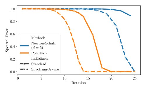
Figure 7: Benefits of the spectrum-aware initialization scheme of Appendix E. Using this scheme improves convergence of both Newton-Schulz and Polar Express on a synthetic matrix with . Note that we count the spectrum-aware initialization as an additional iteration.
图 7:附录 E 中谱感知初始化方案的好处。该方案改善了 Newton-Schulz 和 Polar Express 在一张合成 矩阵()上的收敛。注意我们把谱感知初始化计为额外的一步。
Appendix F Fast Polynomial Iteration for Rectangular Matrices
附录 F 矩形矩阵的快速多项式迭代
In this section, we describe a simple method for applying an iterative polynomial method to a rectangular matrix. For matrices with a large aspect ratio, this method yields significant computational savings. We emphasize that this method is applicable to any computation of the form , where each is an odd polynomial. Thus, it can be used to apply Newton-Schulz or Jordan’s polynomials in addition to our own.
本节描述一种把迭代多项式方法作用到矩形矩阵上的简单办法。对纵横比很大的矩阵,这种方法能带来显著的计算节省。我们强调,该方法适用于任意形如 的计算,其中每个 都是奇次多项式。因此,除了我们自己的多项式之外,它也可以用来作用 Newton-Schulz 或 Jordan 的多项式。
As a preliminary, we first describe the baseline approach. Let with , where is called the aspect ratio. Any odd polynomial of degree can be represented as , where is a polynomial of degree . Thus, . Furthermore, can be written in a factored form called Horner’s rule to reduce the number of multiplications. For instance, if , Horner’s rule gives . For a matrix, . Thus for , computing costs about operations, and computing costs operations. This process could be repeated for each iteration . Notice that if we instead computed , the result would be the same but the cost would be higher.
作为预备,我们先描述基准做法。设 且 ,其中 称为纵横比。任意次数 的奇次多项式 都可以写成 ,其中 是次数为 的多项式。因此 。此外, 可以写成称为 Horner 法则的因式形式,以减少乘法次数。例如,若 ,Horner 法则给出 。对矩阵,。因此对 ,计算 大约花费 次运算,而计算 花费 次运算。这一过程可以对每一步 重复。注意如果我们改算 ,结果相同但代价更高。
A major drawback of this naive approach is that it has a strong dependence on , since two rectangular matrix multiplications must be performed in each of the iterations. When , these two multiplications dominate the cost. In Algorithm 4, we introduce a simple trick that dramatically reduces this cost, using just two rectangular matrix multiplications to compute all iterations.
这种朴素做法的一个主要缺点是对 的依赖很强,因为在全部 步的每一步都必须做两次矩形矩阵乘法。当 时,这两次乘法会主导代价。在算法 4 中,我们引入一个简单技巧来大幅降低这一代价,只用两次矩形矩阵乘法就能完成全部 步。
Let
for do
Horner’s rule:
end for
return
Algorithm 4 Fast Polynomial Iteration for Rectangular Matrices
令
for do
Horner 法则:
end for
return
算法 4 矩形矩阵的快速多项式迭代
To see why this works, define ,
为看清这为何成立,定义 ,
and . It is clear by induction that , and . As promised, this algorithm uses no rectangular multiplications in the for-loop. If each is degree , then the total cost is . When , this is smaller than the naive method. We can use this criterion to select either Algorithm 4 or the baseline method at runtime.
以及 。由归纳法显然有 、,以及 。如所承诺,该算法在 for 循环中不做任何矩形乘法。如果每个 的次数都是 ,则总代价为 。当 时,这比朴素方法更小。我们可以在运行时用这一判据来选择算法 4 或基准方法。
There is one significant weakness of Algorithm 4. In bfloat16 precision, it can introduce numerical errors. Our intuition for why this happens is as follows. Let be the SVD. For large , . Thus, . When has very small singular values and the floating point precision is very low, instantiating may be unstable. To mitigate this issue, we use a restarting strategy. Notice that the issue arises only for large , for which . Limiting ourselves to iterations improves the conditioning of because Thus, to compute iterations, we can apply Algorithm 4 first to the first three polynomials, then again to the last three polynomials. Note that restarting Algorithm 4 after every iteration is exactly the same as the baseline method. This approach provides a tunable hyperparameter—the number of iterations we apply before restarting Algorithm 4—allowing us to find a balance between the fully stable but slow baseline on the one hand, and a very fast but numerically risky method on the other hand.
算法 4 有一个显著弱点。在 bfloat16 精度下,它可能引入数值误差。我们对原因的直觉如下。设 为 SVD。对很大的 ,。因此 。当 有非常小的奇异值且浮点精度很低时,实例化 可能不稳定。为缓解这一问题,我们使用一种重启策略。注意该问题只在 很大、从而 时出现。把自己限制在 步会改善 的条件,因为此时 。因此,要计算 步,我们可以先对前三个多项式应用算法 4,再对后三个多项式再应用一次。注意每一步都重启算法 4,就恰好回到基准方法。这一做法提供了一个可调超参数——在重启算法 4 之前应用的步数——让我们能在一端完全稳定但较慢的基准方法,与另一端非常快但数值上有风险的方法之间取得平衡。
Figure 8 shows that using Algorithm 4 can dramatically improve runtime on the GPU when the aspect ratio is large enough. As expected, using Algorithm 4 for many iterations significantly reduces the dependence of the runtime on the aspect ratio. Running six iterations of a degree-5 polynomial method when (as with the linear transformations in each MLP block of a transformer) we obtain almost a 2x speedup, and when , we obtain nearly a 10x speedup. If we restart every three iterations, the trend is the same but the runtime savings are somewhat smaller.
图 8 表明,当纵横比足够大时,使用算法 4 可以显著改善 GPU 上的运行时间。如所预期,把算法 4 用于许多步,会显著降低运行时间对纵横比的依赖。当 时(正如 Transformer 每个 MLP 块中的线性变换),跑六步五次多项式方法几乎能获得 2 倍加速;当 时,加速接近 10 倍。若每三步重启一次,趋势相同,但运行时间节省会少一些。
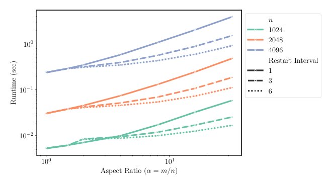
Figure 8: Effects of using Algorithm 4 on runtime on a GPU. We run iterations of a degree-5 polynomial method on matrices with various dimensions and aspect ratios . Restart interval is Algorithm 4, restart interval is equivalent to the baseline (that is, not using Algorithm 4), and restart interval is an intermediate method that calls Algorithm 4 once to do the first three iterations and again to do the last three iterations for greater stability. When , increasing the restart interval significantly reduces the runtime.
图 8:使用算法 4 对 GPU 运行时间的影响。我们在不同维数 和纵横比 的矩阵上,对一种五次多项式方法跑 步。重启间隔 就是算法 4,重启间隔 等价于基准方法(也就是不使用算法 4),重启间隔 是一种中间方法:先调用一次算法 4 做前三步,再调用一次做后三步,以获得更好的稳定性。当 时,增大重启间隔会显著降低运行时间。
Preliminary experiments using Algorithm 4 with Muon in bfloat16 were not successful. The training and validation losses were sometimes significantly higher than before, even accounting for the runtime savings of Algorithm 4. While this technique may already be applicable in float32 or for architectures whose weight matrices have larger aspect rations, more work is needed to make it practical for general deep learning applications.
把算法 4 与 Muon 一起用于 bfloat16 的初步实验并不成功。即便把算法 4 节省的运行时间考虑在内,训练损失和验证损失有时仍显著高于从前。虽然这一技术也许已经可以用于 float32,或用于权重矩阵纵横比更大的架构,但要使它对一般的深度学习应用切实可用,还需要更多工作。
If these problems can be mitigated, the speed afforded by Algorithm 4 suggests a potentially beneficial change in the way Muon is applied to transformers. Each multi-head attention layer contains four square weight matrices and . The orthogonalization step of Muon is either applied separately to these four matrices or else to and , since typical implementations of multi-head attention store the weights in this concatenated form. However, we believe it is natural to consider each of these four weight matrices to be a concatenation of many smaller linear transformations, each corresponding to a single attention head. If is the number of heads, each of these smaller matrices has size ; that is, they have aspect ratio . Since typical transformers like GPT-3 can have as many as heads, this version of Muon can yield huge savings in the runtime of each step. We leave it to future work to examine whether this version of Muon also enjoys fast convergence.
如果这些问题能够缓解,算法 4 带来的速度提示我们,也许可以改变 Muon 作用于 Transformer 的方式。每个多头注意力层包含四个方的权重矩阵 、、 和 。Muon 的正交化步骤要么分别作用于这四个矩阵,要么作用于 和 ,因为多头注意力的典型实现会按这种拼接形式存储权重。不过我们觉得,把这四个权重矩阵各自看成许多更小线性变换的拼接是很自然的,每一个小变换对应一个注意力头。若 是头数,这些较小矩阵的大小为 ;也就是说,它们的纵横比为 。既然像 GPT-3 这样的典型 Transformer 可以有多达 个头,这种版本的 Muon 可以在每一步的运行时间上带来巨大节省。我们把考察这种版本的 Muon 是否同样收敛很快留给未来工作。
Appendix G Code for Constructing Polynomials of Polar Express
附录 G 构造 Polar Express 多项式的代码
The following code gives a Python implementation of the offline stage of Algorithm 2. This code was used to construct the coefficients of the polynomials given in (), which in turn were used in our Muon experiments (Section 5.2). It uses and by default. It incorporates Algorithm 3 and the numerical tweaks described in Section 4.4
下面的代码给出算法 2 离线阶段的一个 Python 实现。这段代码被用来构造 () 中给出的多项式系数,而这些系数又被用于我们的 Muon 实验(第 5.2 节)。它默认使用 和 。它纳入了算法 3 以及第 4.4 节所述的数值调整